the apparent roughness of a sand surface blown by wind ... · pdf filethe open access journal...

The apparent roughness of a sand surface blown by wind from an analytical model of saltation

This article has been downloaded from IOPscience. Please scroll down to see the full text article.

2012 New J. Phys. 14 043035

(http://iopscience.iop.org/1367-2630/14/4/043035)

Download details:

IP Address: 108.38.27.71

The article was downloaded on 26/04/2012 at 04:34

Please note that terms and conditions apply.

View the table of contents for this issue, or go to the journal homepage for more

Home Search Collections Journals About Contact us My IOPscience

http://iopscience.iop.org/page/terms

http://iopscience.iop.org/1367-2630/14/4

http://iopscience.iop.org/1367-2630

http://iopscience.iop.org/

http://iopscience.iop.org/search

http://iopscience.iop.org/collections

http://iopscience.iop.org/journals

http://iopscience.iop.org/page/aboutioppublishing

http://iopscience.iop.org/contact

http://iopscience.iop.org/myiopscience

T h e o p e n – a c c e s s j o u r n a l f o r p h y s i c s

New Journal of Physics

The apparent roughness of a sand surface blown bywind from an analytical model of saltation

T Pahtz1, J F Kok2,3 and H J Herrmann1,3

1 Computational Physics, IfB, ETH Zurich, Schafmattstrasse 6,8093 Zurich, Switzerland2 Department of Earth and Atmospheric Sciences, Cornell University,1104B Bradfield Hall, Ithaca, NY 14850, USA3 Departamento de Fısica, Universidade Federal do Ceara, 60451-970 Fortaleza,Ceara, BrazilE-mail: [email protected], [email protected] and [email protected]

New Journal of Physics 14 (2012) 043035 (43pp)Received 5 November 2011Published 25 April 2012Online at http://www.njp.org/doi:10.1088/1367-2630/14/4/043035

Abstract. We present an analytical model of aeolian sand transport. The modelquantifies the momentum transfer from the wind to the transported sand byproviding expressions for the thickness of the saltation layer and the apparentsurface roughness. These expressions are derived from basic physical principlesand a small number of assumptions. The model further predicts the sand transportrate (mass flux) and the impact threshold (the smallest value of the wind shearvelocity at which saltation can be sustained). We show that, in contrast toprevious studies, the present model’s predictions are in very good agreementwith a range of experiments, as well as with numerical simulations of aeoliansaltation. Because of its physical basis, we anticipate that our model will findapplication in studies of aeolian sand transport on both Earth and Mars.

New Journal of Physics 14 (2012) 0430351367-2630/12/043035+43$33.00 © IOP Publishing Ltd and Deutsche Physikalische Gesellschaft

mailto:[email protected]



http://www.njp.org/

2

Contents

1. Introduction 42. Model description 6

2.1. Notations and definitions . . . . . . . . . . . . . . . . . . . . . . . . . . . . . 72.2. Grain shear stress profile . . . . . . . . . . . . . . . . . . . . . . . . . . . . . 92.3. Force balance . . . . . . . . . . . . . . . . . . . . . . . . . . . . . . . . . . . 102.4. Work rate balance . . . . . . . . . . . . . . . . . . . . . . . . . . . . . . . . . 122.5. Invariance of α and β . . . . . . . . . . . . . . . . . . . . . . . . . . . . . . . 142.6. A novel relation for zs . . . . . . . . . . . . . . . . . . . . . . . . . . . . . . . 142.7. Physical meaning of zs . . . . . . . . . . . . . . . . . . . . . . . . . . . . . . 162.8. Calculation of z∗

0 . . . . . . . . . . . . . . . . . . . . . . . . . . . . . . . . . 172.9. Closing the model: a relation for ut . . . . . . . . . . . . . . . . . . . . . . . . 21

3. Model validation 223.1. Experimental validation . . . . . . . . . . . . . . . . . . . . . . . . . . . . . . 233.2. Independence of the model parameters with atmospheric and grain properties . 23

4. Discussion 30Acknowledgments 31Appendix A. Supplementary information 31Appendix B. Comparison between the scaling law of Andreotti and the numerical

data 33Appendix C. Computing impact and lift-off velocities with the model of Kok 34Appendix D. Calculation of the average wind velocity profile and the apparent

roughness 34Appendix E. Surface roughness of a quiescent sand bed 40References 42

Nomenclature

z height above the sand bed = vertical coordinatex horizontal coordinate in the direction of the wind flowu∗ fluid shear velocityκ von Karman constantu(z) average vectorial wind velocity at height zz∗

0 apparent roughness of the transported saltation layerz0 surface roughness of a quiescent sand bedg gravity constantg buoyancy-reduced gravity constantvl average lift-off velocityθl average lift-off anglevi average impact velocityθi average impact angleh average saltation heightzr height of the low-energy layerut impact threshold = shear velocity above which saltation can be sustained

New Journal of Physics 14 (2012) 043035 (http://www.njp.org/)

http://www.njp.org/

3

cc1, cc2, cc3, correlation factorscc4, cc5

zs decay height of an exponentially decreasing grain shear stress profileτg(z) grain shear stress profileτgo τgo = τg(0)

d mean particle diameterρs particle densityρw air densitys s = ρs/ρw

µ dynamic viscosity of airQ saltation mass fluxα the first model parameter and force ratioα the modified first model parameter if vertical drag is consideredβ the second model parameter and proportional to β

β square root of work rate ratioγ the third model parameter, γ = zm/zs

zm effective height of the mean motionη the fourth model parameter, defined by (71)ρ(z) transported mass per volume at height zρo ρo = ρ(0)

M transported mass per unit soil areav↑(↓) average vectorial velocity of upward (downward) moving particlesvxo↑(↓) vxo↑(↓) = vx↑(↓)(0)

vzo↑(↓) vzo↑(↓) = vz↑(↓)(0)

vr(z) u(z) − v(z)1vx(z), 1vz(z), velocity differences defined by (10)–(13)1v2

x(z), 1v2z (z)

1vxo, 1vzo, 1vx(0), 1vz(0), 1v2x(0), 1v2

z (0)

1v2xo,1v2

zoφ(z) local vertical mass flux at height zφo φo = φ(0)

pg(z) grain normal stress profilepgo pgo = pg(0)

f sum of the average vectorial drag force and gravityCd(V ) drag coefficient as a function of velocity difference VCo parameter in the drag lawC∞ C∞ = Cd(∞)

ez unit vector in the z-directionV r V r = U − VV average particle velocityV 2

z V 2z = 〈v2

z 〉

U U = u(zm)

G function defined by (60)Fγ function defined by (66)H function defined by (D.30)E1 function defined by (59)


http://www.njp.org/

4

Ein function defined by (D.12)3F2 generalized hypergeometric seriesua(z) reduced shear velocity profile, defined by (58)ub ub = ua(0)

Vo average particle slip velocity, Vo = (ρo↑vxo↑ + ρo↓vxo↓)/ρo

V t V t = V (ut)

U t U t = U (ut)

zmt zmt = zm(ut)

τ wind shear stress, τ = ρwu2∗

a a = τgo/τ

f j Taylor coefficients of 1 −√

1 − xK (a) function defined by (D.16)I infinite sum defined by (D.24)S(l)

k Stirling numbers of the second kindg f effective gravity incorporating the effect of cohesionζ dimensional cohesion parameterRek roughness Reynolds number

1. Introduction

The dominant mechanism of aeolian sand transport, i.e. the transport of sand due to air flow,is the process of saltation, in which the wind accelerates sand grains that hop along thesurface. During their hops, the sand particles continuously exchange momentum with the wind.Therefore the wind momentum decreases, resulting in reduced wind velocities not only withinbut also above the saltation layer. Above the saltation layer, the average horizontal wind velocityprofile u(z) follows the well-known law [1]

u(z) =u∗

κln

z

z∗

0

, (1)

where κ = 0.4 is the von Karman constant and z∗

0 is the apparent roughness of the movingsaltation layer. The wind shear velocity u∗ =

√τ/ρw is the velocity scale resulting from the

shear stress τ applied by the wind with density ρw onto the sand surface. In the absence ofsand transport, z∗

0 becomes z0, which is the surface roughness of a quiescent sand bed. In thepresence of sand transport, the magnitude of z∗

0 depends on how much momentum is absorbedby the saltation layer.

It is crucial for the development of sand transport models, but also for landscape modelersand coastal managers, to know z∗

0 as a function of u∗ and z0. For instance, z∗

0 is a key quantity inaeolian dune models for the computation of the wind field over non-flat topography, for whichthe shear velocity u∗ varies with the spatial position [2–6].

The main purpose of this paper therefore is to derive a novel prediction of z∗

0 which ismainly based on physical principles.

Previous studies have also attempted to derive a scaling law for z∗

0. The first importantcontribution to this matter came from Owen [7]. His study suggested that

z∗

0 ∝u2

∗

g, (2)


http://www.njp.org/

5

where g is the gravitational constant. (Equation (2) is also known as the Charnock relation sinceCharnock [8] derived (2) for the roughness of a wind-blown water surface.) Owen [7] basedhis formula on the following assumptions: that the average lift-off velocity vl with which agrain leaves the bed is proportional to u∗, that vertical friction with the air can be neglectedand that z∗

0 is proportional to the average hop height of grains h, also called saltation height.However, the author’s assumptions are inconsistent with recent measurements. In particular,experimental studies [9–12] found vl, and consequently h, to be almost independent of u∗.Furthermore, z∗

0 cannot be proportional to h since z∗

0 was found to strongly vary with u∗ inexperiments [13–15], in contrast to h. In addition, Sherman [16] found that (2) leads to largediscrepancies with experiments close to the impact threshold ut, which is the threshold shearvelocity at which saltation can be sustained through the splash process [17]. On Earth, ut isbelow the fluid entrainment shear velocity needed to entrain sand grains from the soil by fluidlift [1, 18]. Sherman [16] therefore extended (2) to the so-called modified Charnock relation,

z∗

0 − z0 ∝(u∗ − ut)

2

g, (3)

which ensures that at the threshold u∗ = ut, where no particles are moving, the roughness isunchanged, z∗

0 = z0. Although (3) was successfully validated with the data set of Sherman andFarrell [15] for z∗

0, it shares the same lack of physical justification as (2).A more physical relation for the apparent roughness of the saltation layer was presented by

Raupach [19]. Using the mixing length approximation [20], the author derived

lnz∗

0

z0=

(1 −

ut

u∗

)ln

zs

1.78z0, (4)

where zs is the decay height of the grain shear stress profile τg(z), which the author assumed tobe exponentially decreasing,

τg(z) = τgo e−z/zs, (5)

where τgo = τg(0). τg(z) describes how much momentum is transferred, at each height z, fromthe fluid to the grains per unit soil area and time. The difficulty in the usage of (4) is theundetermined quantity zs. Raupach [19] therefore assumed that zs is proportional to the saltationheight h, and that h is in turn proportional to u2

∗/g like Owen [7] before him. However, as we

discussed before, Owen’s assumption is inconsistent with experiments.Relations very similar to (4) were also obtained in the studies of Andreotti [21] and Duran

and Herrmann [22]. These studies obtained agreement with the wind tunnel measurements ofz∗

0 by Rasmussen et al [13] by fitting zs in (4) to these measurements. Andreotti [21] found thatthe data set can be fitted well if zs scales with

√d , where d is the mean particle diameter, and

he therefore suggested

zs ∝√

sgd

(µ

ρwg2

)1/3

, (6)

where s = ρs/ρw is the ratio of sand density ρs to fluid density ρw, and µ is the dynamicviscosity. A scaling law very similar to (6) was also used by Duran and Herrmann [22].However, (6) was not derived from physical principles, but rather it was postulated based onthe resulting agreement of (4) with the data set of Rasmussen et al [13] for z∗

0. It is thereforeunclear whether the scaling with s, µ, ρw and g describes the physics correctly. Therefore, thereis a necessity to either validate (6) or derive a new expression for zs from physical principles.


http://www.njp.org/

6

Within this study we do the latter. We do so by presenting an analytical model of aeoliansaltation in the steady state, which, for the first time, provides expressions for zs and z∗

0 that arederived from basic physical principles and a small number of assumptions. The model derives,furthermore, expressions for other important sand transport quantities, such as the saltation massflux Q and the impact threshold ut. We thus consider our model to be an improvement overprevious analytical models.

We validate our model with several experimental data sets: measurements of the apparentroughness data by Rasmussen et al [13] for five different grain sizes, measurements of theimpact threshold from several studies [17, 23, 24] and measurements of the saltation massflux by Creyssels et al [11]. Furthermore, we test our expressions for conditions for whichexperiments are not available using simulations with the numerical saltation model of Kok andRenno [25], for instance by varying ρw, µ or g. These comparisons with both experiments andsimulations support our model and suggest that all model parameters (α, β, γ and η) are nearlyindependent of u∗, the atmospheric conditions, as well as g and d.

The paper is structured as follows. It starts with a comprehensive model description insection 2, followed by model validation in section 3 and a discussion of results in section 4. Theappendices incorporate detailed calculations and supplemental information. We have includeda glossary in order to help the reader keep track of the various mathematical symbols.

2. Model description

As discussed in the introduction, the main purpose of our paper is to derive a novel expressionfor the apparent roughness z∗

0 during aeolian sand transport in steady state. The main focus ofour model is therefore on the analytical description of the momentum and energy transfer fromthe wind to the grains, since this produces an increase of the surface roughness z0 of a quiescentsand bed to the apparent roughness z∗

0 of a moving saltation layer.The model is based on the concept of mean motion, meaning that average quantities are

used for its description. We separately consider the horizontal and vertical transport of grains.For each, we analytically balance the average force and work rate exerted by the wind withthe respective amounts exerted during an impact onto the soil. This results in the parameters α,describing the ratio between the average vertical and horizontal forces per unit soil area, andβ, describing the ratio between the average work rate per unit soil area in the vertical motionand that in the horizontal motion. We use theoretical arguments to show that α and β are nearlyindependent of u∗ and the atmospheric conditions, and only slightly dependent on the buoyancy-reduced gravity g and the particle diameter d. The model further contains a third parameter γ ,defined as the ratio between zs and the height of mean motion zm, and a fourth parameter η,describing the ratio between the average particle velocity reduced by the particle slip velocityand the average wind velocity. The final relations for zs, z∗

0 and Q are functions of α, β, γ andut, whereby ut is a function of α, β, γ and η, and β is a model parameter proportional to β.

For the balance laws, we only consider wind drag and gravity as driving forces, and thusneglect lift forces, electrostatic forces, as well as mid-air collisions between grains. We do soboth to keep the analysis simple and because gravity and drag dominate the sand transport [25].We further simplify the description by only considering time-averaged quantities, which impliesthat we neglect turbulent fluctuations of the wind velocities. Further assumptions are the use ofmonodisperse, spherical sand grains, and a horizontal sand bed. Possibly the most crucial ofthese simplifications is the neglecting of mid-air collisions between saltating grains, the effects


http://www.njp.org/

7

of which remain poorly understood [26–29]. Many previous analytical and numerical studieshave also neglected mid-air collisions, e.g. [11, 21, 25, 30].

In addition to these simplifications, we use a few working assumptions in our model. Wemainly assume that the model parameters are nearly constant, and that the grain shear stressprofile τg(z) is decaying exponentially with height z, as previous studies did [19, 22] (see (5)).

This section is organized into several subsections. It starts with the presentation of notationsand definitions that are used for the description of our model in section 2.1. In section 2.2 therefollows a short discussion of our main model assumption, the exponentially decreasing grainshear stress profile. After that, the balance laws are applied, first for the force per unit soil areain section 2.3 and then for the work rate per unit soil area in section 2.4. Subsequently, wediscuss the invariance of the parameters α and β in section 2.5. Afterwards, we obtain a novelrelation for zs in section 2.6, which is further discussed in section 2.7. Then in section 2.8 therelations for z∗

0 and Q as a function of ut and the model parameters are obtained. In section 2.9,the model is extended to include the computation of ut as well.

2.1. Notations and definitions

For the below analytical calculations, we henceforth use the following notations: the index xrefers to the horizontal component of a given quantity, which coincides with the direction ofthe wind, and the index z to the vertical direction, whereby z is also the height above the sandbed. Furthermore, we differentiate between the upward and downward parts of a grain’s hopby indices ↑ and ↓, respectively. Quantities evaluated at the sand bed (z = 0) incorporate anadditional index o. In particular, quantities which refer to a grain’s impact consist of the indiceso and ↓ if the quantity is evaluated before the impact, but of the indices o and ↑ if the quantityis evaluated after the impact.

In order to keep the paper simple, it is advantageous to predefine quantities which are usedin the following calculations. One quantity is the average particle mass per unit volume ρ(z),transported at height z. ρ(z) integrated over the whole saltation layer describes the mass M oftransported sand per unit soil area,

M =

∫∞

0ρ(z) dz. (7)

The height z = 0 at which the integration starts is thereby defined by means of the undisturbedvelocity profile, (1) with z∗

0 = z0. Specifically, we define z = 0 as being a height z0 below thezero point of the undisturbed wind velocity profile. Experiments in water flumes over a sedimentbed show that this height is approximately located at the top of the topmost sediment layer(see van Rijn [31], figure 2.2.3). Consequently, sand grains in the bed are not included in thecomputation of M since their central point is below z = 0.

Since we differentiate between the upward and downward movement, ρ(z) can be dividedinto the mass of upward- and downward-moving particles per unit volume

ρ(z) = ρ↑(z) + ρ↓(z). (8)

Other important quantities are the average vectorial wind velocity profile, u(z), whose z-component is zero u(z) = ux(z) = |u(z)|, and the average vectorial particle velocity profile forthe upward (downward) part of the hop v↑(↓)(z) (see figure 1). The difference between bothvelocities is denoted as

vr↑(↓)(z) = u(z) − v↑(↓)(z). (9)


http://www.njp.org/

8

Figure 1. Sketch of ρ↑(↓) and v↑(↓)(z). The fading red color indicates a decreaseof ρ↑(↓) with increasing z.

Based on these definitions, we further define the following velocity differences by

1vx(z) = vx↓(z) − vx↑(z), (10)

1vz(z) = vz↓(z) − vz↑(z) (11)

and

1v2x(z) = v2

x↓(z) − v2

x↑(z), (12)

1v2z (z) = v2

z↓(z) − v2z↑(z), (13)

as well as the local vertical mass flux φ(z) by

φ(z) = ρ↑(z)vz↑(z) = −ρ↓(z)vz↓(z), (14)

where we used that the vertical upward flux must exactly compensate for the downwardflux in the steady state. Note that vz↓(z) and thus 1vz(z) are negative. Using (8), (14) can berewritten as

φ(z) = ρ(z)vz↓(z)vz↑(z)

1vz(z). (15)

With these definitions, the average gain of the horizontal and the vertical momentum of atransported grain per unit soil area and the time between the two times it crosses height z canbe written as

τg(z) = φ(z)1vx(z) (16)

for the horizontal and

pg(z) = φ(z)1vz(z) (17)

for the vertical momentum gain per unit soil area and time. τg(z) is also known as the grain shearstress profile [19, 22, 30] and pg(z) can be interpreted as a grain normal stress (grain pressure)profile. Note that, by inserting (15) in (17), one obtains

pg(z) = ρ(z)vz↓(z)vz↑(z), (18)


http://www.njp.org/

9

10−4

10−2

1000

0.05

0.1

0.15

0.2

0.25

0.3

Grain shear stress, τg [N/m2]

Height,z[m]

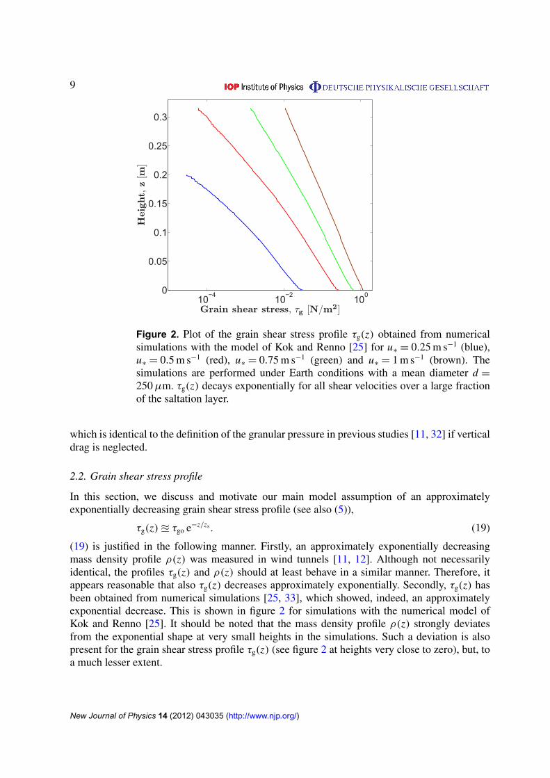
Figure 2. Plot of the grain shear stress profile τg(z) obtained from numericalsimulations with the model of Kok and Renno [25] for u∗ = 0.25 m s−1 (blue),u∗ = 0.5 m s−1 (red), u∗ = 0.75 m s−1 (green) and u∗ = 1 m s−1 (brown). Thesimulations are performed under Earth conditions with a mean diameter d =

250 µm. τg(z) decays exponentially for all shear velocities over a large fractionof the saltation layer.

which is identical to the definition of the granular pressure in previous studies [11, 32] if verticaldrag is neglected.

2.2. Grain shear stress profile

In this section, we discuss and motivate our main model assumption of an approximatelyexponentially decreasing grain shear stress profile (see also (5)),

τg(z)u τgo e−z/zs . (19)

(19) is justified in the following manner. Firstly, an approximately exponentially decreasingmass density profile ρ(z) was measured in wind tunnels [11, 12]. Although not necessarilyidentical, the profiles τg(z) and ρ(z) should at least behave in a similar manner. Therefore, itappears reasonable that also τg(z) decreases approximately exponentially. Secondly, τg(z) hasbeen obtained from numerical simulations [25, 33], which showed, indeed, an approximatelyexponential decrease. This is shown in figure 2 for simulations with the numerical model ofKok and Renno [25]. It should be noted that the mass density profile ρ(z) strongly deviatesfrom the exponential shape at very small heights in the simulations. Such a deviation is alsopresent for the grain shear stress profile τg(z) (see figure 2 at heights very close to zero), but, toa much lesser extent.


http://www.njp.org/

10

2.3. Force balance

Having discussed our main model assumption in section 2.2, we now begin to introduce ouranalytical model, which starts with a force balance. As already pointed out, the description ofthe momentum transfer from the wind to the grains via fluid forces is a key ingredient towarda description of the feedback effect of sand transport on the wind profile and thus a first steptoward a prediction of the apparent roughness z∗

0.We use a fluid description for the momentum balance. The momentum balance for an

upward (downward)-moving volume Vt↑(↓) of transported sand can be written as

d

dt

∫Vt↑(↓)

ρ↑(↓)v↑(↓)dV =

∫Vt↑(↓)

f↑(↓)dV, (20)

where f↑(↓) is the average vectorial force per unit volume acting on the grains in the upward(downward) motion. The index ‘t’ in Vt↑(↓) indicates that the volume is changing in time t sinceit is moving with the average particle velocity v↑(↓). Since we use the concept of mean motion,contributions from local fluctuations of the particle velocity around the mean value v↑(↓) areneglected in (20). We now use the Reynolds transport theorem [34] to move the derivation d/dtinto the integrand of the left-hand side of (20). This yields

∂(ρ↑(↓)v↑(↓))

∂t+ ∇ · (ρ↑(↓)v↑(↓)v↑(↓)) = f↑(↓), (21)

where we dropped the integration since (20) is valid for arbitrary volumes Vt. For steady-statesaltation (∂/∂x = 0, ∂/∂t = 0), (21) becomes

d

dz(ρ↑(↓)vz↑(↓)vx↑(↓)) = fx↑(↓), (22)

d

dz(ρ↑(↓)vz↑(↓)vz↑(↓)) = fz↑(↓). (23)

Summing the upward and downward parts of (22) and (23), respectively, using (14), (16)and (17), and integrating over height finally yields

τg(z) = φ(z)1vx(z) =

∫∞

zfx(z

′) dz′, (24)

pg(z) = φ(z)1vz(z) =

∫∞

zfz(z

′) dz′, (25)

where f = f↑ + f↓ is the total vectorial force acting on the grains. If evaluated at z = 0, the termson the left-hand side of (24) and (25) describe the average horizontal and vertical force per unitsoil area applied by the soil on the grains during an impact and the right-hand side the averagehorizontal and vertical force per unit soil area applied by the wind on the grains during theirhops, respectively. In the next steps, we evaluate the integrals in (24) and (25) at z = 0 in orderto obtain the ratio between the total horizontal and vertical force per unit soil area acting on thegrains. To do so, we first need an expression for the total force f. Since we neglect lift forces andmomentum transfer through collisions, f is only composed of the drag force on monodisperse


http://www.njp.org/

11

and spherical grains with diameter d, and the gravity force, which acts in the z-direction sincewe consider a nearly horizontal sand bed. The total force f can therefore be written as

f =3

4sd

(ρ↑Cd(vr↑)vr↑vr↑ + ρ↓Cd(vr↓)vr↓vr↓

)− ρ gez, (26)

where ez is the unit vector in the z-direction, g =s−1

s g with s = ρs/ρw is the buoyancy-reducedgravity (for most atmospheres g u g), and vr↑(↓) = |vr↑(↓)|. Cd is the drag coefficient, which isa function of the particle Reynolds number and therefore of vr↑(↓). Since gravity is generallymuch larger than vertical drag, we approximate fz as

fz u−ρ g. (27)

However, note that we do not use this approximation in section 2.4 since there the effect ofgravity vanishes. Further note that the effect of vertical drag on the force balance is discussedin appendix A.1. On the other hand, we rewrite fx as

fx =3ρ

4sd〈Cd(vr)vrvrx〉, (28)

where 〈〉 denotes a weighted average of a quantity f between the upward and downwardmovement, 〈 f 〉 = (ρ↑ f↑ + ρ↓ f↓)/ρ.

Now we evaluate the integrals in (24) and (25) using the expressions we derived for fx andfz, respectively. We obtain

τgo = τg(0) =

∫∞

0

3ρ

4sd〈Cd(vr)vrvrx〉 dz =

3M〈Cd(vr)vrvrx〉

4sd(29)

and

pgo = pg(0) = −gM, (30)

where the overbar denotes the average of a quantity f over height, f =∫

∞

0 ρ f dz/M .With the evaluation of the integrals, we can now define our first model parameter α as

α = −pgo

τgo=

−1vzo

1vxo=

4sgd

3〈Cd(vr)vrvrx〉, (31)

where we have used (16) and (17) as well as the notations 1vxo = 1vx(0) and 1vzo = 1vz(0).The advantage of this definition of α lies in the fact that it is almost independent of u∗,atmospheric conditions, g and d, as we show later in section 2.5. We can thus formulate relevantsand transport quantities as a function of a constant α. For instance, using (30) and (31), weobtain a direct relation between the grain shear stress τgo at the bed and the mass of transportedgrains per unit soil area M , writing

τgo = α−1gM. (32)

Furthermore, we can approximately calculate the average velocity difference V r as a functionof α. For this purpose, we first approximate

〈Cd(vr)vrvrx〉 = cc1Cd(V r)V rV rx u cc1Cd(V r)V2r . (33)

For the equal sign on the left-hand side of (33), we evaluated the average of the function as acorrelation factor cc1 times the function of the averages, and for the approximation on the right-hand side, we used V rx u V r, which seems reasonable since in aeolian saltation the horizontalmotion dominates the vertical one [35]. Correlation factors such as cc1 do not change much


http://www.njp.org/

12

with conditions if the functional shapes of the averaged quantities, here vrx↑(↓)(z) and vr↑(↓)(z),do not change much. In this particular case, we neglect the correlations from the averagingprocedure, cc1 u 1, in order to keep the number of final model parameters to a minimum.Note that we also tested the performance of the final model using the validation proceduredescribed in section 3, and using cc1 as an additional model parameter. We found that the modelperformance is not affected significantly if 0.85 < cc1 < 1.15, but decreases for values of cc1

outside this range. This suggests that the actual value of cc1 is, indeed, close to unity, and thatsmall errors from neglecting the correlation in this particular case can be incorporated in theother model parameters.

Using cc1 = 1, we now obtain a direct relation between the average velocity difference V r

and α from (31) and (33), writing

Cd(V r)V2r =

4sgd

3α. (34)

2.4. Work rate balance

The second important ingredient towards a description of the feedback effect of the grain motionon the wind profile and toward a prediction of z∗

0 is the description of the energy transfer fromthe fluid to the grains.

In order to obtain a work rate balance, we multiply (22) and (23) by the respective termsinside the derivation on the left-hand sides. Using chain rule for the derivatives, this yields

1

2

d

dz(ρ↑(↓)vz↑(↓)vx↑(↓))

2= fx↑(↓)ρ↑(↓)vz↑(↓)vx↑(↓), (35)

1

2

d

dz(ρ↑(↓)vz↑(↓)vz↑(↓))

2= fz↑(↓)ρ↑(↓)vz↑(↓)vz↑(↓). (36)

The work rate balances with respect to the horizontal and vertical motions can now be obtainedby subtracting the upward from the downward parts of (35) and (36), respectively, using (14),and integrating over height. It yields

1

2φ(z)21v2

x(z) =

∫∞

zφ(z′)( fx↑vx↑ + fx↓vx↓)(z

′) dz′, (37)

1

2φ(z)21v2

z (z) =

∫∞

zφ(z′)( fz↑vz↑ + fz↓vz↓)(z

′) dz′. (38)

If evaluated at z = 0 and divided by φo = φ(0), the terms on the left-hand side of (37) and (38)describe the average work rate during an impact and the right-hand side the average work rateduring a hop for the horizontal and vertical motions, respectively. Since gravity does not dowork, we cannot use the approximation (27) which neglects vertical drag. If (27) were insertedin (38), the right-hand side would vanish due to (14) and the left-hand side due to 1v2

z = 0; thismeans that information would be lost. Therefore, we use the more accurate form of fz givenby (26) and obtain

fx↑vx↑ + fx↓vx↓ =3ρ

4sd〈Cd(vr)vrvrxvx〉, (39)

fz↑vz↑ + fz↓vz↓ = −3ρ

4sd〈Cd(vr)vrv

2z 〉. (40)


http://www.njp.org/

13

10−3

10−2

10−1

1000

0.1

0.2

0.3

0.4

0.5

0.6

0.7

Normalized particle concentration, ρ/ρo

Height,z[m]

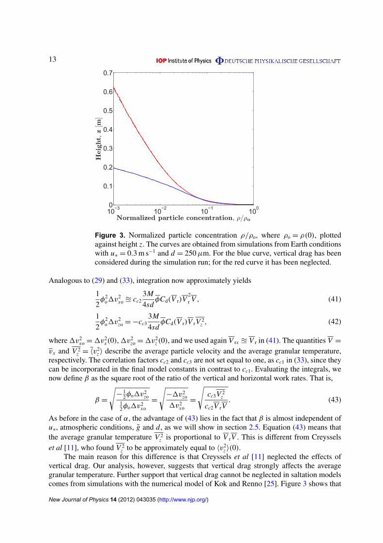
Figure 3. Normalized particle concentration ρ/ρo, where ρo = ρ(0), plottedagainst height z. The curves are obtained from simulations from Earth conditionswith u∗ = 0.3 m s−1 and d = 250 µm. For the blue curve, vertical drag has beenconsidered during the simulation run; for the red curve it has been neglected.

Analogous to (29) and (33), integration now approximately yields

1

2φ2

o1v2xo u cc2

3M

4sdφCd(V r)V

2r V , (41)

1

2φ2

o1v2zo = −cc3

3M

4sdφCd(V r)V rV 2

z , (42)

where 1v2xo = 1v2

x(0), 1v2zo = 1v2

z (0), and we used again V rx u V r in (41). The quantities V =

vx and V 2z = 〈v2

z 〉 describe the average particle velocity and the average granular temperature,respectively. The correlation factors cc2 and cc3 are not set equal to one, as cc1 in (33), since theycan be incorporated in the final model constants in contrast to cc1. Evaluating the integrals, wenow define β as the square root of the ratio of the vertical and horizontal work rates. That is,

β =

√−

12φo1v2

zo12φo1v2

xo

=

√−1v2

zo

1v2xo

=

√cc3V 2

z

cc2V rV. (43)

As before in the case of α, the advantage of (43) lies in the fact that β is almost independent ofu∗, atmospheric conditions, g and d, as we will show in section 2.5. Equation (43) means thatthe average granular temperature V 2

z is proportional to V rV . This is different from Creysselset al [11], who found V 2

z to be approximately equal to 〈v2z 〉(0).

The main reason for this difference is that Creyssels et al [11] neglected the effects ofvertical drag. Our analysis, however, suggests that vertical drag strongly affects the averagegranular temperature. Further support that vertical drag cannot be neglected in saltation modelscomes from simulations with the numerical model of Kok and Renno [25]. Figure 3 shows that


http://www.njp.org/

14

the rescaled density profile decays much more slowly with z if vertical drag is considered (bluecurve), compared to the case when vertical drag is neglected (red curve).

2.5. Invariance of α and β

Since our model relations, including the final relation for z∗

0, will be expressed as functions of α

and β, it is important to discuss how these parameters change with varying conditions. As canbe seen from (31) and (43), both parameters are ratios of velocity differences evaluated at thesoil z = 0, and are therefore related to the entrainment of bed particles through particle impacts,or ‘splash’. In aeolian steady state saltation, splash entrainment is the dominant mechanismresponsible for setting grains of the sand bed into motion (see section 2.3 in [36]). The otherpotentially relevant mechanism, the entrainment of bed grains by the wind itself, is generally oflittle importance in steady state saltation, since the wind shear velocity at the surface is belowthe fluid entrainment threshold and even decreases with increasing u∗ [22, 36].

A salton impact on the particle bed can have different outcomes. The impacting grain mayrebound or settle. At the same time it may destabilize bed grains so strongly that they are ejectedfrom the bed. Since the particle concentration remains constant in steady state, the impact ratemust be balanced by the sum of the rebound and ejection rates. In other words, each impactinggrain must, on average, lead to exactly one grain leaving the surface through either reboundor the ejection of new grains. The average number of grains leaving the surface per impactinggrain can, however, only depend on the average impact velocity vi , angle θi and relevant bedproperties, such as g and d . Furthermore, for given values of g and d, the average velocity vl

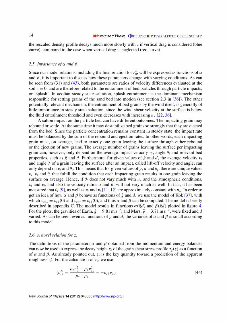
and angle θl of a grain leaving the surface after an impact, called lift-off velocity and angle, canonly depend on vi and θi . This means that for given values of g, d and θi , there are unique valuesvi , vl and θl that fulfill the condition that each impacting grain results in one grain leaving thesurface on average. Hence, if θi does not vary much with u∗ and the atmospheric conditions,vi and vl , and also the velocity ratios α and β, will not vary much as well. In fact, it has beenmeasured that θi [9], as well as vi and vl [11, 12] are approximately constant with u∗. In order toget an idea of how α and β behave as functions of g and d , we use the model of Kok [37], withwhich vzo↓ = vz↓(0) and vzo↑ = vz↑(0), and thus α and β can be computed. The model is brieflydescribed in appendix C. The model results in functions α(gd) and β(gd) plotted in figure 4.For the plots, the gravities of Earth, g = 9.81 m s−2, and Mars, g = 3.71 m s−2, were fixed and dvaried. As can be seen, even as functions of g and d , the variance of α and β is small accordingto this model.

2.6. A novel relation for zs

The definitions of the parameters α and β obtained from the momentum and energy balancescan now be used to express the decay height zs of the grain shear stress profile τg(z) as a functionof α and β. As already pointed out, zs is the key quantity toward a prediction of the apparentroughness z∗

0. For the calculation of zs, we use

〈v2z 〉 =

ρ↑v2z↑ + ρ↓v

2z↓

ρ↑ + ρ↓

= −vz↑vz↓, (44)


http://www.njp.org/

15

0.0001 0.001 0.01

0.8

0.85

0.9

0.95

gd [m2/s2]

Forceratio,α

(a) (b)

0.0001 0.001 0.01

0.25

0.27

0.29

0.31

0.32

gd [m2/s2]

Squarerootoftheworkrateratio,β

Figure 4. The force ratio α (blue) and the square root of the work rate ratio β

(red) computed with the model of Kok [37] (see appendix C) and plotted versusgd . Gravity was set to either the Earth (solid lines) or the Mars value (dashedlines), and d was varied.

where we inserted (14). We further approximate the arithmetic average of |vz↑| and |vz↓| by theirgeometric average

−1vz

2=

|vz↑| + |vz↓|

2u√

|vz↑||vz↓| =√

−vz↑vz↓, (45)

which seems reasonable since |vz↑|/|vz↓| < |vzo↑|/|vzo↓|, and measurements indicate that|vzo↑|/|vzo↓| is about 1.5 [38], which means that the error of this approximation is less than3%. Using (15), (16), (44) and (45), we express τg as

τg = φ1vx =ρvz↑vz↓

1vz1vx u

1

2ρ

√〈v2

z 〉1vx . (46)

This allows us to rewrite (24) as

−dτg

dzu

τg

zs=

ρ√

〈v2z 〉1vx

2zs= fx =

3ρ

4sd〈Cd(vr)vrvrx〉, (47)

where we used (19). Note that (47) is an approximation. In particular, it can be invalid veryclose to the ground, where the grain shear stress can deviate from the exponential profile due tothe creep flux (see figure 2 at heights very close to zero). In order to obtain an expression thatcharacterizes the decay height zs over most of the saltation layer, we average (47) over height.We therefore approximately calculate zs as

zs u2sd

√〈v2

z 〉1vx

3〈Cd(vr)vrvrx〉=

αcc41Vx

√V 2

z

2g= αβ

V12r V

32

g, (48)

where we used (31), (43), and√

〈v2z 〉1vx = cc41Vx

√V 2

z . cc4 is another correlation factor and

β = βcc4√

cc21Vx/(2√

cc3V ). β is our second model parameter and, like β, is approximatelyindependent of u∗ and the atmospheric conditions since we expect that 1vx is to leading order


http://www.njp.org/

16

10−3

10−2

10−1

1000

0.05

0.1

0.15

0.2

0.25

0.3

0.35

Normalized profiles, ρ/ρo and τg/τgo

Height,z[m]

zr

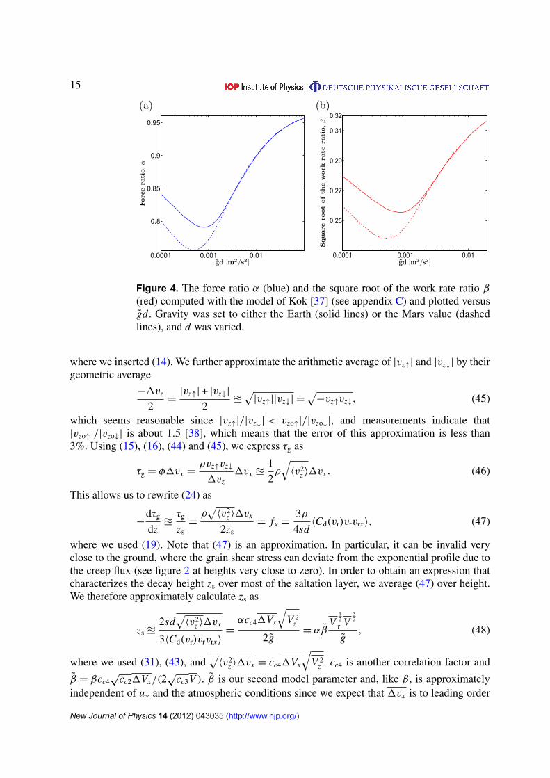
Figure 5. The normalized profiles τg/τgo (solid lines) and ρ/ρo (dashed lines)plotted versus height z for Earth conditions with d = 250 µm and two differentshear velocities, u∗ = 0.3 m s−1 (blue) and u∗ = 0.8 m s−1 (red).

proportional to V , and that the correlation factors do not change much with conditions. Weconsider (48) to be the main contribution of our paper since it is, to our knowledge, the firstphysically based prediction of zs and therefore the most important step toward a novel physicallybased prediction of z∗

0. If the values of the model parameters α and β are known, V remains theonly undetermined quantity in (48) since V r can be calculated by (34) as a function of α. There isevidence that zs does not only describe the decay of τg(z), but also the decay of ρ(z) for heightsz above a certain cut-off height zr. This is shown in figure 5 for simulations with the numericalmodel of Kok and Renno [25]. Since the profile ρ(z)/M describes the distribution of the locationof saltating grains, zs is related to the saltation height h, which is the average hop height of thegrains. However, the relation between h and zs is not obvious since figure 5 also shows that thedecaying behavior of ρ(z) is very different from τg(z) below the cut-off height zr, where ρ(z)decays much more strongly than the exponential decrease above zr. This deviation from theexponential shape was also found for mass flux profiles q(z) = ρ(z)〈vx〉(z) by Namikas [9] infield experiments. Since the change of 〈vx〉(z) with z is very small in comparison to the changeof ρ(z), we conclude that this deviation of ρ(z) is also present in Namikas’ [9] experiments. Inthe following section, we discuss the relation between zs and h.

2.7. Physical meaning of zs

It was assumed in previous studies that zs and the saltation height h are proportional toeach other [19, 21, 22]. In this section, we show, by calculating h, that this assumption isinconsistent with our model. In order to calculate h, we use that φ(z)/φo describes the fractionof grains which have a lift-off velocity large enough to reach height z [39, 40]. Consequently,P(z) = −φ−1

o dφ/dz must describe the distribution of hop heights of grains. The average value


http://www.njp.org/

17

of z weighted with P(z) must therefore describe the average hop height h. That is,

h = −1

φo

∫∞

0z

dφ(z)

dzdz =

1

φo

∫∞

0φ(z)dz u

1

ρo

√〈v2

zo〉

∫∞

0ρ(z)

√〈v2

z 〉dz =

cc5

√V 2

z

ρo

√〈v2

zo〉M,

(49)

where cc5 is another correlation factor, 〈v2zo〉 = 〈v2

z 〉(0), we used partial integration and weapproximated φ = τg/1vx u 1

2ρ√

〈v2z 〉 using (16) and (46). Now, using (18) and (44), we

express pg as

pg = −ρ〈v2z 〉. (50)

Furthermore, using (30) and (50), M can be expressed as M = ρo〈v2zo〉/g, which inserted in (49)

and using (43) gives

h = cc5

√〈v2

zo〉

√V 2

z

g= βcc5

√cc2

cc3

√〈v2

zo〉

√V rV

g. (51)

Having calculated h, we can now compare our expression for zs (48) with (51). Clearly, ouranalysis suggests that zs and h are not proportional to each other. But if zs does not describe theaverage hop height of grains, what else does it describe? In order to answer this question, werecall that zs approximately describes the exponential decay of ρ(z) for z > zr, as discussed inthe previous section. Since ρ(z)/M describes the distribution of the location of saltating grains,it seems reasonable to interpret zs as the expected location of grains with hop heights larger thanzr, which we call high-energy saltons. The expected location of high-energy saltons can, in turn,be interpreted as a measure for the thickness of the saltation layer. In contrast to zs, the cut-offheight zr should be proportional to the expected location of grains with hop heights smaller thanzr, which we call low-energy saltons.

Our analysis confirms the picture of Andreotti [21], who hypothesized that one canessentially distinguish two species in aeolian saltation: low-energy saltons (reptons) slowlymoving in small hops and high-energy saltons moving fast in large hops. The authorhypothesized that zr is a measure for the height of the focal region, a region in which steadystate wind profiles for different shear velocities u∗ intersect.

Note that the decay height zs (48) as well as the saltation height h (51) change with V andthus with u∗. The prediction of V is therefore the subject of the following subsection.

2.8. Calculation of z∗

0

The last step toward the calculation of z∗

0 is to derive an expression for V , the last undeterminedquantity in (48), our relation for zs. zs is the main parameter in our final relation for z∗

0, whichwill be of a similar structure as (4), the relation of Raupach [19]. For deriving V , we use thefollowing strategy.

Due to the mean value theorem of integration, U must be equal to the wind velocity at anintermediate height zm, which we call the height of mean motion. Using this, we first calculateU = u(zm) with the mixing length approximation [20], and then we compute V by

V = U − V r, (52)

where we use that V r does not change with u∗ (see (34)). Finally, we assume that zm isproportional to zs, and we explain why we do so.


http://www.njp.org/

18

Following the outlined strategy, we calculate U from the mixing length approximation[19, 20, 22, 30, 33] as

du(z)

dz=

u∗

κz

√1 −

τg(z)

ρwu2∗

, (53)

with

u(z0) = 0. (54)

In the absence of sand transport, τg(z) = 0, the mixing length approximation yields theundisturbed logarithmic velocity profile ((1) with z∗

0 = z0). In the presence of sand transport,τg(z)> 0, the velocity profile deviates from the logarithmic shape. In appendix D, we calculateu(z) and z∗

0 based on our model assumption of an exponentially decreasing grain shear stressprofile (19). This calculation approximately yields

lnz∗

0

z0=

(1 −

ub

u∗

)ln

zs

1.78z0− G

(ub

u∗

)(55)

and for z > 0.1zs

u(z) =u∗

κln

z

z∗

0

+u2

∗− u2

b

2κu∗

E1

(z

zs

), (56)

where ub is the reduced wind shear velocity at the bed, defined by

ub = ua(0), (57)

ua(z) = u∗

√1 −

τg(z)

ρwu2∗

, (58)

and the exponential integral E1(x) as well as G(x) are defined by

E1(x) =

∫∞

x

e−x ′

x ′dx ′

= −0.577 − ln x +∞∑

l=1

(−1)l+1x l

ll!, (59)

G(x) = 1.154(1 + x ln x)(1 − x)2.56. (60)

Note that (56) is only an approximation of u(z) for z > 0.1zs. In appendix D, we also providedan approximation for z < zs, which, however, has a much more complicated structure. Forthe coming calculations, we are only interested in the value U = u(zm), for which bothapproximations perform well since zm is between 0.1zs and 0.4zs as we show later.

In (55) and (56) the shear velocity at the bed ub remains undetermined. It was shown byUngar and Haff [40] that ub must decrease with u∗, starting from ub(ut) = ut. The reason isthat one observes a focal region in an aeolian steady-state saltation, called the Bagnold focus,below which the wind velocities decrease with increasing u∗ [1, 41]. Andreotti [21] arguedthat the presence of the Bagnold focus and consequently the value of ub are mainly caused bygrains transported in the low-energy layer. As we explained in sections 2.2 and 2.6, the massdensity profile ρ(z) and also the grain shear stress profile τg(z) deviate from the exponentialdecrease within the low-energy layer z � zr. We, however, used this exponential decrease ofτg(z) (see (19)), our main model assumption, for the computation of the apparent roughness andthe wind profile in (55) and (56). This does not mean that (55) and (56) are wrong, because the


http://www.njp.org/

19

0 2 4 6 810

−3

10−2

10−1

100

101

Wind speed, u [m/s]

Normalizedheight,z/z s

z=0.1zs

0 2 4 6 8 1010

−3

10−2

10−1

100

101

Wind speed, u [m/s]

Normalizedheight,z/z s

z=0.1zs

(a) (b)

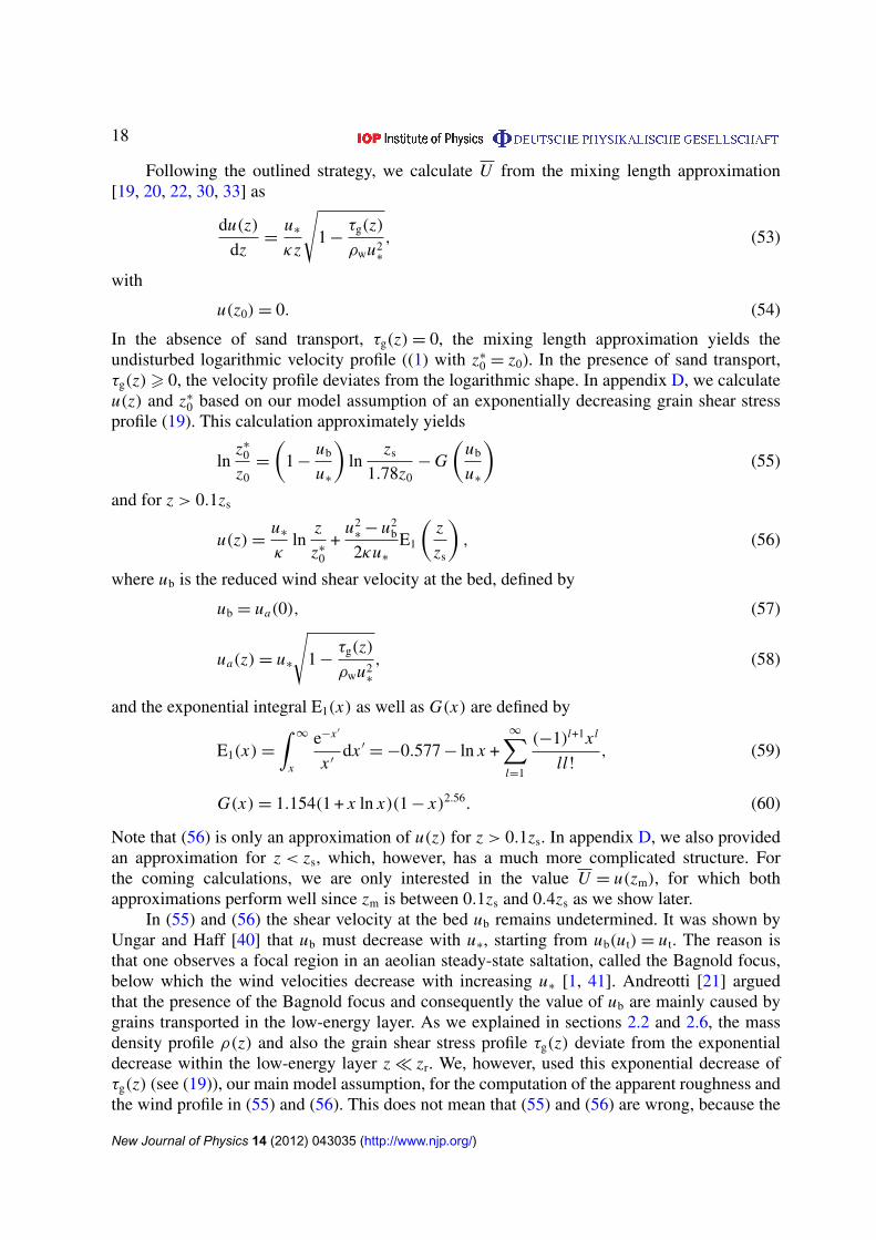
Figure 6. The wind speed u plotted against z/zs for the Mars conditions withd = 250 µm and two different shear velocities, u∗ = 0.39 m s−1 (a) and u∗ =

0.59 m s−1 (b). The solid lines show the simulated wind profiles [25], whereas thedashed lines show the wind profiles computed by (55) and (56). In (55) and (56),we inserted the values of zs, which we obtained from fitting to the simulatedgrain shear stress profiles τg(z). The blue color differs from the red color only inthe value of ub. For the blue curves, ub = ut is used, whereas for the red curves,the simulated values of ub are used.

deviation of τg(z) from the exponential shape is very small (almost invisible in figure 2). Butit means that we cannot use the real value of ub, which is influenced by the low-energy layer.Instead, we must use a value of ub that corresponds to the extrapolation of the exponential shapeof τg(z) above z = zr to the height z = 0. Such a value of ub would be larger than the real valuebecause ρ(z) and thus τg(z) deviate from the exponential shape towards higher values withinthe low-energy layer. We therefore propose that this value is close to ut,

ub u ut. (61)

This approximation is supported by simulations using the numerical model of Kok andRenno [25]. Figure 6 shows that wind profiles calculated by (56) with the hypothesis (61)are much closer to the simulated profiles than those in which the simulated values of ub wereused, and this although this hypothesis eliminates the Bagnold focus. In particular, in the regionin which we are interested, z > 0.1zs, (55) and (56) provide an excellent approximation ofthe simulated wind profile, when using (61). Note that (61) is also known as Owen’s secondhypothesis, and it has been used in many previous models, e.g. [7, 19, 30, 35, 42]. Nonetheless,Owen’s hypothesis is known to be physically incorrect [36], but its use is justified in ourparticular application due to the ‘cancellation of errors’ with the deviation of τg(z) from theexponential profile in the low-energy layer.

From (55), (56) and (61) we now obtain

lnz∗

0

z0=

(1 −

ut

u∗

)ln

zs

1.78z0− G

(ut

u∗

)(62)


http://www.njp.org/

20

and

U =u∗

κln

zm

z∗

0

+u2

∗− u2

t

2κu∗

E1(γ ), (63)

where γ is the third model parameter, defined by

γ =zm

zs. (64)

The first terms on the right-hand side of (55) and (62) are identical to the relations of previousstudies [19, 22] (see also (4)). The second term appears because we did not approximate theright-hand side of (53) before the integration as done in these studies. Our solution is thereforemore precise. Note that the height of mean motion zm should be in leading order proportionalto the decay height zs of the grain shear stress profile because the mean motion is dominated bythe motion of high-energy saltons [21], and zs is a measure for the height of high-energy saltons(see section 2.7). Consequently, we assume that γ is constant.

Before we calculate V in order to close (48), we rewrite (63) more elegantly. For thispurpose, we define zmt = zm(ut), U t = U (ut) = κ−1(u)t ln(zmt/z0), and V t = V (ut), and usezm/zmt = (V /V t)

1.5 (see (48)). Then, inserting (62) in (63) and using ln(zm/z0) = ln(zmt/z0) +1.5 ln(V /V t), we obtain

U = U t +3ut

2κln

V

V t

+u∗

κFγ

(ut

u∗

), (65)

where the function Fγ (x) is defined by

Fγ (x) = (1 − x) ln(1.78γ ) + 0.5(1 − x2)E1(γ ) + G(x). (66)

Having obtained a relation for U , we can now calculate V with (52), insert V in (48) toobtain zs and insert zs in (62) to obtain z∗

0. The calculation of z∗

0 can therefore be summarized as

lnz∗

0

z0=

(1 −

ut

u∗

)ln

zs

1.78z0− G

(ut

u∗

), (67a)

zs = αβV

12r V

32

g, (67b)

V = V t +3ut

2κln

V

V t

+u∗

κFγ

(ut

u∗

), (67c)

V t =ut

κln

αβγ V12r V

32t

gz0− V r, (67d)

Cd(V r)V2r =

4sgd

3α, (67e)

where we used (52) and (65) for (67c), and (48), (52) and (64) for (67d). Equations (67a),(67b) and (67e) are identical to (62), (48) and (34), respectively. Given a certain drag lawCd(V ), (67c), (67d) and (67e) can be solved iteratively for V , V t and V r, respectively. Thisis our novel prediction of z∗

0 in the most general version. If the impact threshold ut is known,z∗

0 can be calculated using (67a)–(67e) as a function of the model parameters α, β and γ .


http://www.njp.org/

21

It is further possible to compute the mass flux Q as a function of the same parameters. Forthis purpose, we first compute the mass of transported sand per unit soil area M from (32)and (61) as

M =αρw

g(u2

∗− u2

t ). (68)

Then the mass flux Q becomes

Q =

∫∞

0ρ(z)vx(z)dz = MV =

αρw

g(u2

∗− u2

t )V . (69)

At the moment all model equations are functions of the model parameters and ut. In orderto close the model, ut must be calculated as a function of the model parameters as well. This isdone in the following with the help of a closing assumption.

2.9. Closing the model: a relation for ut

Equations (67a)–(67e) are already a novel expression for z∗

0. Like previous expressions in theliterature (see (2)–(4) and (6)), our expression requires the impact threshold ut as an inputparameter. We therefore close the model by deriving a relation for ut in this section. Our strategyis as follows. We first motivate a simple expression for the particle velocity at the threshold,V t. We then compute V r = U t − V t and combine the result with our previous expression forV r (67e). The resulting equation can be rearranged to compute ut.

As outlined in the previous paragraph, we motivate the following closing expression:

V t = ηU t + Vo = ηut

κln

zmt

z0+ Vo, (70)

where Vo = (ρo↑vxo↑ + ρo↓vxo↓)/ρo is the average particle slip velocity (i.e. the particle speed atthe surface), where vxo↑(↓) = vx↑(↓)(0) and ρo↑(↓) = ρ↑(↓)(0), and η is the fourth model parameter.Equation (70) means that the difference between the average particle and slip velocities underthreshold conditions is proportional to the average wind velocity. This is justified in thefollowing manner. The particle slip velocity Vo is a quantity that, like the parameters α and β,only depends on the impact-entrainment process. In particular, Vo is independent of the averagewind velocity U t. From theoretical and experimental studies it is known that the profile ofthe average horizontal particle velocity vx(z) starts with Vo at z = 0 and increases with heightz [11, 12, 25]. The average increase with z mainly depends on the average wind velocity U t.Consequently, the average particle velocity V t is a function of the average wind velocity U t

plus an offset Vo. The simplest possible relation with such a behavior is given by (70). Therebyη describes how efficiently the wind accelerates transported grains under threshold conditions.Rearranging (70), η can be written as

η =V t − Vo

U t

. (71)

In order to close expression (70), an expression for Vo is required. Since Vo is determinedby the splash process, it is predominantly controlled by the velocity scale

√gd [11]. However, at

small grain diameters d, cohesive interparticle forces make it more difficult for impacting grainsto eject bed particles, such that the impact and lift-off velocities, and thus Vo, must increase.


http://www.njp.org/

22

These forces can be accounted for by replacing the velocity scale√

gd with√

g f d [37, 43],where

g f = g +6ζ

πρsd2(72)

is an effective gravity and ζ = 5 × 10−4 N m−1 a dimensional parameter (see appendix C). Wetherefore model Vo as

Vo = 16.2√

g f d, (73)

where the prefactor 16.2 ensures that Vo = 1 m s−1 as measured by Creyssels et al [11] ford = 242 µm and g = 9.81 m s−2. Note that it is also possible to calculate the particle slip velocityVo with the model of Kok [37], explained in appendix C; however, for the sake of simplicity weuse (73).

Now we can use (70) to calculate V r. According to (67e), V r does not depend on u∗. Wecan therefore write

V r = V r(ut) = U t − V t = (1 − η)ut

κln

zmt

z0− Vo, (74)

Rearranging and using (48), (64) and (70) finally yields an expression for ut, which can besummarized as

ut =κ(V r + Vo)

(1 − η) ln zmtz0

, (75a)

zmt =αβγ V

12r V

32t

g, (75b)

V t =Vo + ηV r

1 − η, (75c)

Cd(V r)V2r =

4sgd

3α. (75d)

3. Model validation

We validate our expressions (67a)–(67e), (69) and (75a)–(75d) by showing that the same setof model parameters can explain the following experiments: the mass flux data of Creysselset al [11], the apparent roughness data of Rasmussen et al [13] and the combined impactthreshold data of different studies [17, 23, 24].

We further evaluate our model using simulations with the numerical saltation model of Kokand Renno [25], which has been validated by a range of measurements. The simulation resultsevaluate (67a)–(67e), (68) and (74) for many different conditions including environments forwhich experiments are unavailable. For instance, experiments have never been performed onMars where the fluid density ρw, the gravity g and fluid viscosity µ are very different from theEarth values. Using these simulations also gives us the possibility of testing our expressions forparticular quantities that have never been measured, such as the functional dependences of Mand zs on u∗. Another advantage of using numerical simulations is that they provide data thathave a much smaller scatter than experimental data. Nevertheless, using simulation data bears


http://www.njp.org/

23

the risk that the model on which they are based does not describe the physics sufficiently well.Agreement between our model and the numerical simulations is therefore only an indicator ofthe correctness of our model.

We use the simulations in order to confirm our statements that the model parameters α andβ are approximately independent of the shear velocity and atmospheric conditions, and furtherindicate that γ and η also do not vary much. That is, we show that all model parameters adoptapproximately the same values for whatever conditions are simulated.

In order to compute V r in (67e) and (75d), we use in the following the drag law ofCheng [44] for natural sand grains:

Cd(V ) =

((32µ

Vρwd

)2/3

+ 1

)3/2

. (76)

3.1. Experimental validation

For the validation with experiments, we need to account for the fact that the surface roughnessz0 of a quiescent sand bed is a function of the roughness Reynolds number. This is particularlyimportant when making a comparison with experimental impact thresholds, because someexperiments were done with very small particle diameters d in the aerodynamically smoothregime. We discuss this issue in appendix E, which also provides the equations that we use tocompute z0.

In this section, we validate our apparent roughness prediction (67a)–(67e) with theexperiments of Rasmussen et al [13] for five different particle diameters d . The chosen data sethas the advantage that the scatter in the data is small in comparison to other data sets [14, 15].Furthermore, we use a combination of several data sets [17, 23, 24] in order to evaluate ourimpact threshold prediction (75a)–(75d), and we use the data set of Creyssels et al [11] to testour mass flux prediction (69). The latter choice is motivated by the fact that Creyssels et al [11]used a large wind tunnel (15 m length), which decreases the influence of finite-size effects onthe mass flux Q. For instance, the two mass flux measurements of Iversen and Rasmussen [45]and Ho et al [12], which were made in a smaller wind tunnel (6 m length), show magnitudesof Q that are ≈ 1.5–2.5 times smaller than Q measured by Creyssels et al [11], although theseexperiments used the same sand and equipment. We want to emphasize that we use only a singleset of parameters α, β, γ and η to fit all data sets at the same time, and that the values of ut,obtained from our prediction (75a)–(75d), are used in (67a)–(67e) and (69).

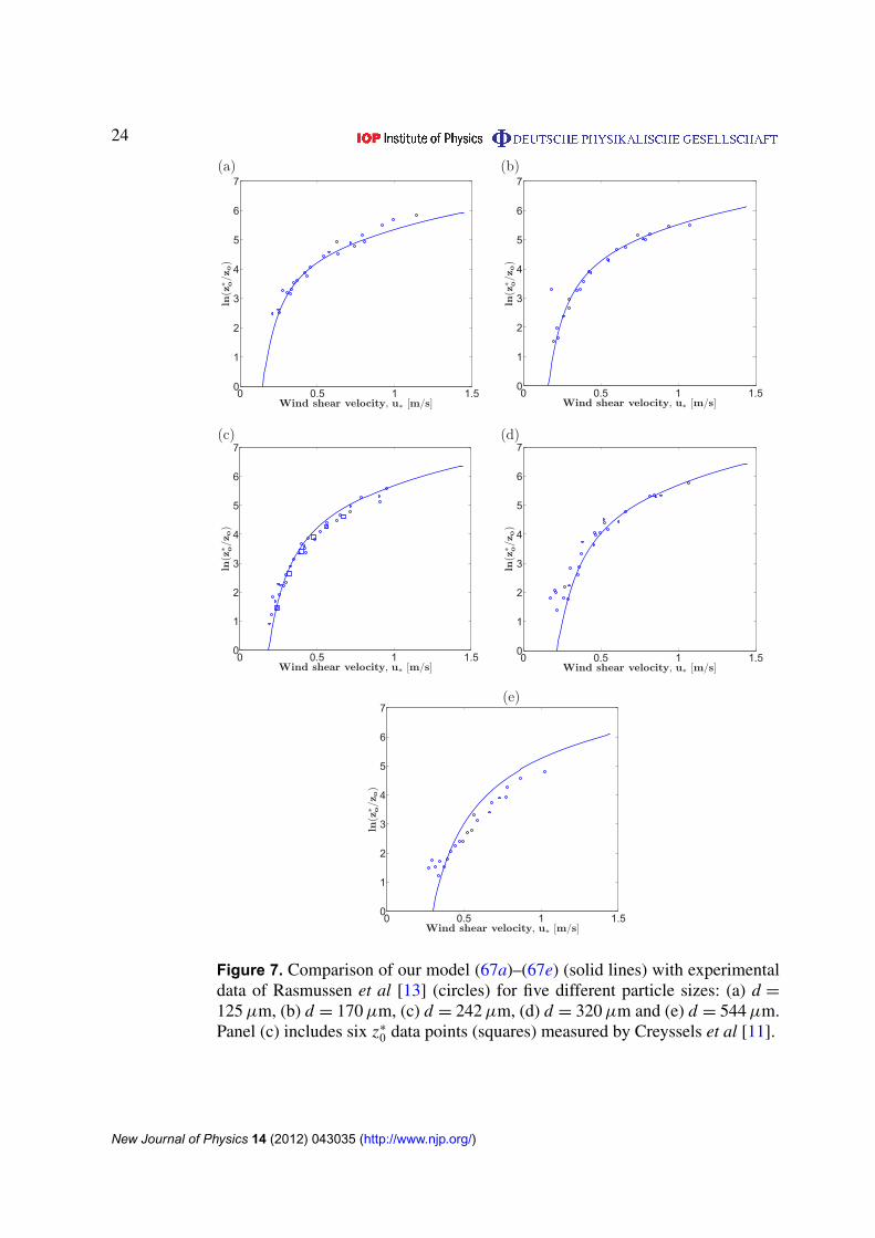
By fitting the model parameters to α = 1.02, β = 0.095, γ = 0.17 and η = 0.1, we obtaingood agreement with all data sets. This is shown in figures 7–9, which present the comparisonof (67a)–(67e) with the data of Rasmussen et al [13], the comparison of (75a)–(75d) with theimpact threshold data sets [17, 23, 24], and the comparison of (69) with the mass flux data ofCreyssels et al [11], respectively.

3.2. Independence of the model parameters with atmospheric and grain properties

For the verification of the independence of the model parameters we use simulation results ofthe numerical model of Kok and Renno [25] for a range of atmospheric and grain properties,as summarized in table 1. The fluid density ρw, viscosity µ and particle densities ρs are varied


http://www.njp.org/

24

0 0.5 1 1.50

1

2

3

4

5

6

7

Wind shear velocity, u∗ [m/s]

ln(z∗ o/z o)

0 0.5 1 1.50

1

2

3

4

5

6

7


ln(z∗ o/z o)

0 0.5 1 1.50

1

2

3

4

5

6

7


ln(z∗ o/z o)

0 0.5 1 1.50

1

2

3

4

5

6

7


ln(z∗ o/z o)

0 0.5 1 1.50

1

2

3

4

5

6

7


ln(z∗ o/z o)

(a) (b)

(c) (d)

(e)

Figure 7. Comparison of our model (67a)–(67e) (solid lines) with experimentaldata of Rasmussen et al [13] (circles) for five different particle sizes: (a) d =

125 µm, (b) d = 170 µm, (c) d = 242 µm, (d) d = 320 µm and (e) d = 544 µm.Panel (c) includes six z∗

0 data points (squares) measured by Creyssels et al [11].


http://www.njp.org/

25

101

102

1030.1

0.2

0.3

0.4

0.5

Mean grain diamter, d [µm]

Impactthreshold,ut[m/s]

ModelBagnold (1937)Chepil (1945)Iversen & Rasmussen (1994)

Figure 8. Comparison of our model (75a)–(75d) (solid line) with experimentaldata [17, 23, 24] (symbols).

0.2 0.3 0.4 0.5 0.6 0.70

0.02

0.04

0.06

0.08

0.1


Massflux,Q[kg/(ms)]

Figure 9. Comparison of our model (69) (solid line) with experimental data ofCreyssels et al [11] (circles).

between the Earth and Mars values, and the particle diameter d is varied between 100 and500 µm. The surface roughnesses z0 in the absence of saltation are chosen to be z0 = d/30,except for two cases (z0 = d/10 and z0 = d/90), which allows us to check whether the predictiveperformance of our model equations is sensitive to the value of z0.


http://www.njp.org/

26

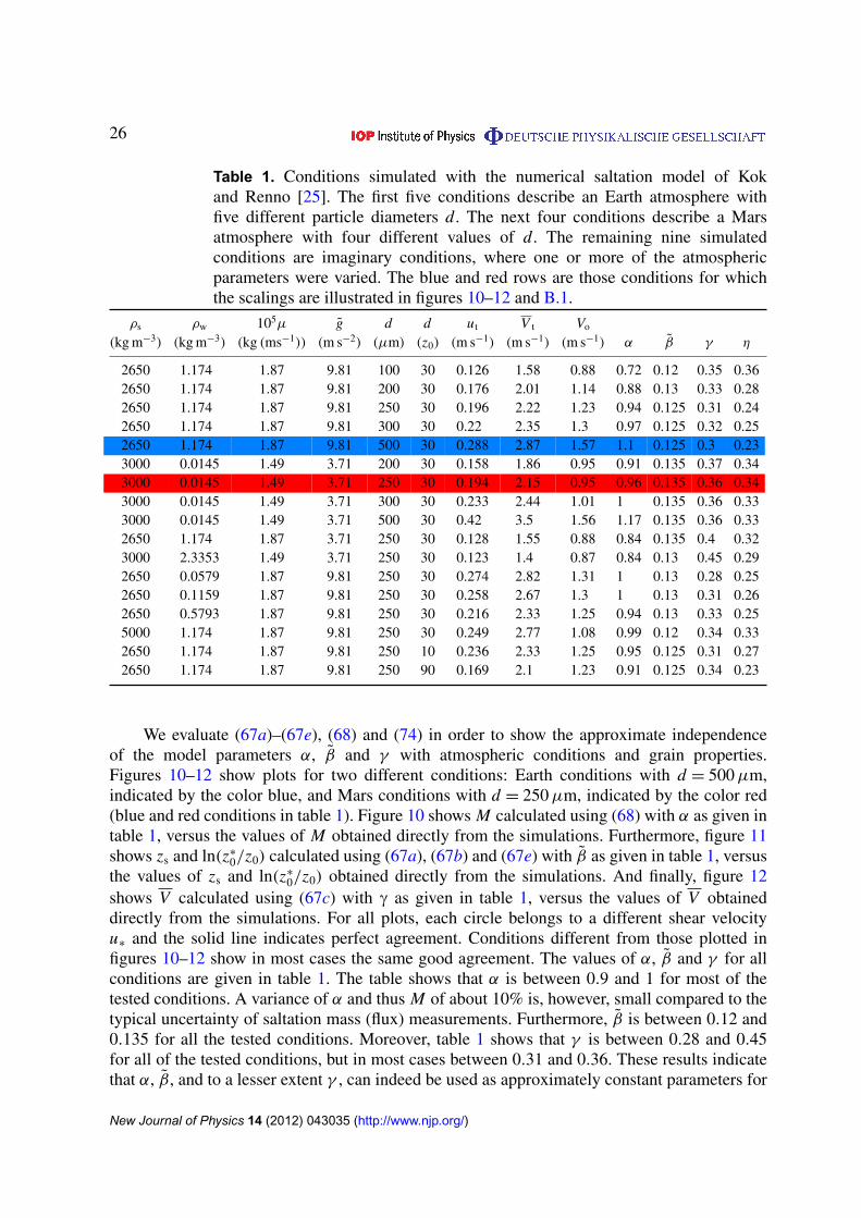
Table 1. Conditions simulated with the numerical saltation model of Kokand Renno [25]. The first five conditions describe an Earth atmosphere withfive different particle diameters d. The next four conditions describe a Marsatmosphere with four different values of d. The remaining nine simulatedconditions are imaginary conditions, where one or more of the atmosphericparameters were varied. The blue and red rows are those conditions for whichthe scalings are illustrated in figures 10–12 and B.1.

ρs ρw 105µ g d d ut V t Vo

(kg m−3) (kg m−3) (kg (ms−1)) (m s−2) (µm) (z0) (m s−1) (m s−1) (m s−1) α β γ η

2650 1.174 1.87 9.81 100 30 0.126 1.58 0.88 0.72 0.12 0.35 0.362650 1.174 1.87 9.81 200 30 0.176 2.01 1.14 0.88 0.13 0.33 0.282650 1.174 1.87 9.81 250 30 0.196 2.22 1.23 0.94 0.125 0.31 0.242650 1.174 1.87 9.81 300 30 0.22 2.35 1.3 0.97 0.125 0.32 0.252650 1.174 1.87 9.81 500 30 0.288 2.87 1.57 1.1 0.125 0.3 0.233000 0.0145 1.49 3.71 200 30 0.158 1.86 0.95 0.91 0.135 0.37 0.343000 0.0145 1.49 3.71 250 30 0.194 2.15 0.95 0.96 0.135 0.36 0.343000 0.0145 1.49 3.71 300 30 0.233 2.44 1.01 1 0.135 0.36 0.333000 0.0145 1.49 3.71 500 30 0.42 3.5 1.56 1.17 0.135 0.36 0.332650 1.174 1.87 3.71 250 30 0.128 1.55 0.88 0.84 0.135 0.4 0.323000 2.3353 1.49 3.71 250 30 0.123 1.4 0.87 0.84 0.13 0.45 0.292650 0.0579 1.87 9.81 250 30 0.274 2.82 1.31 1 0.13 0.28 0.252650 0.1159 1.87 9.81 250 30 0.258 2.67 1.3 1 0.13 0.31 0.262650 0.5793 1.87 9.81 250 30 0.216 2.33 1.25 0.94 0.13 0.33 0.255000 1.174 1.87 9.81 250 30 0.249 2.77 1.08 0.99 0.12 0.34 0.332650 1.174 1.87 9.81 250 10 0.236 2.33 1.25 0.95 0.125 0.31 0.272650 1.174 1.87 9.81 250 90 0.169 2.1 1.23 0.91 0.125 0.34 0.23

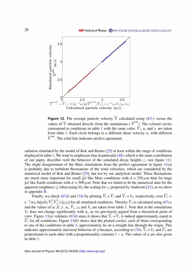
We evaluate (67a)–(67e), (68) and (74) in order to show the approximate independenceof the model parameters α, β and γ with atmospheric conditions and grain properties.Figures 10–12 show plots for two different conditions: Earth conditions with d = 500 µm,indicated by the color blue, and Mars conditions with d = 250 µm, indicated by the color red(blue and red conditions in table 1). Figure 10 shows M calculated using (68) with α as given intable 1, versus the values of M obtained directly from the simulations. Furthermore, figure 11shows zs and ln(z∗

0/z0) calculated using (67a), (67b) and (67e) with β as given in table 1, versusthe values of zs and ln(z∗

0/z0) obtained directly from the simulations. And finally, figure 12shows V calculated using (67c) with c as given in table 1, versus the values of V obtaineddirectly from the simulations. For all plots, each circle belongs to a different shear velocityu∗ and the solid line indicates perfect agreement. Conditions different from those plotted infigures 10–12 show in most cases the same good agreement. The values of α, β and γ for allconditions are given in table 1. The table shows that α is between 0.9 and 1 for most of thetested conditions. A variance of α and thus M of about 10% is, however, small compared to thetypical uncertainty of saltation mass (flux) measurements. Furthermore, β is between 0.12 and0.135 for all the tested conditions. Moreover, table 1 shows that γ is between 0.28 and 0.45for all of the tested conditions, but in most cases between 0.31 and 0.36. These results indicatethat α, β, and to a lesser extent γ , can indeed be used as approximately constant parameters for


http://www.njp.org/

27

10−4

10−2

10−4

10−2

Calculated Mass, αρwg−1(u2∗ − u2t ) [kg/m2]

SimulatedMass,Msim[kg/m2]

Figure 10. The particle mass M per unit soil area calculated using (68), versusthe values of M obtained directly from the simulations (M sim). The coloredcircles correspond to conditions in table 1 with the same color. α, ρw and g aretaken from table 1. Each circle belongs to a different simulated shear velocity u∗

with a different M sim. The solid line indicates perfect agreement.

0.13 0.15 0.17 0.19

0.13

0.15

0.17

0.19

zpreds = αβg−1V0.5r (V

sim)1.5 [m]

Calculated decay height

Simulateddecayheight,zsim s[m]

0 1 2 3 4 5 6 70

1

2

3

4

5

6

7

(1−ut/u

*)ln(z

spred/(1.78z

o))−G(u

t/u

*)

ln(z

o*sim

/zo)

(a) (b)

Figure 11. The decay height of the grain shear stress profile zs (a) and ln(z∗

0/z0)

(b) calculated using (67a), (67b) and (67e) versus zsims and ln(z∗sim

0 /z0), thevalues of zs and ln(z∗

0/z0) obtained directly from simulations. The colored circlescorrespond to conditions in table 1 with the same color. α, β, g and ut are takenfrom table 1. V r is calculated using (67e) with the values of ρs, ρw, µ and d fromtable 1. Each circle belongs to a different shear velocity u∗ with different zsim

s ,

ln(z∗sim0 /z0) and V

sim, the value of V obtained directly from the simulations. The

solid line indicates perfect agreement.


http://www.njp.org/

28

2 2.5 3 3.52

2.5

3

3.5

Vpred= V t + 1.5κ−1ut ln(V

pred/V t) + κ−1u∗Fγ(ut/u∗)

Calculated particle velocity [m/s]

Simulatedparticlevelocity

Vsim[m/s]

Figure 12. The average particle velocity V calculated using (67c) versus thevalues of V obtained directly from the simulations ( V

sim). The colored circles

correspond to conditions in table 1 with the same color. V t, ut and γ are takenfrom table 1. Each circle belongs to a different shear velocity u∗ with differentV

sim. The solid line indicates perfect agreement.

saltation simulated by the model of Kok and Renno [25] at least within the range of conditionsdisplayed in table 1. We want to emphasize that in particular (48), which is the main contributionof our paper, describes well the behavior of the simulated decay heights zs (see figure 11).The slight disagreement of the Mars simulations from the perfect agreement in figure 11(a)is probably due to turbulent fluctuations of the wind velocities, which are considered by thenumerical model of Kok and Renno [25], but not by our analytical model. These fluctuationsare much more important for small gd like Mars conditions with d = 250 µm than for largegd like Earth conditions with d = 500 µm. Note that we failed to fit the numerical data for theapparent roughness z∗

0 when using (6), the scaling for zs proposed by Andreotti [21], as we showin appendix B.

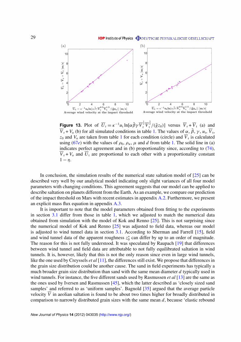
Finally, we check (67d) and (74) by plotting V r + V t and V r + Vo, respectively, over U t =

κ−1(u)t ln[αβγ V12r V

32t /(gz0)] for all simulated conditions. Thereby V r is calculated using (67e),

and the values of α, β, γ , ut, V t, z0 and Vo are taken from table 1. Note that in the simulationsVo does not change significantly with u∗ as we previously argued from a theoretical point ofview. Figure 13(a) validates (67d) since it shows that V r + V t is indeed approximately equal toU t for all conditions. Figure 13(b) shows that the plotted circles, each of them correspondingto one of the conditions in table 1, approximately lie on a straight line through the origin. Thisindicates approximately universal behavior of η because, according to (74), V r + Vo and U t areproportional to each other with a proportionality constant 1 − η. The values of η are also givenin table 1.


http://www.njp.org/

29

0 2 4 6 8 100

2

4

6

8

10

Ut = κ−1utln[αβγV0.5r V

1.5t /(gzo)] [m/s]

Average wind velocity at the impact threshold

Ut=Vr+Vt[m/s]

0 2 4 6 8 100

2

4

6

8

10

Ut = κ−1utln[αβγV0.5r V

1.5t /(gzo)] [m/s]

Average wind velocity at the impact threshold

Vr+Vo[m/s]

(a) (b)

Figure 13. Plot of U t = κ−1ut ln[αβγ V12r V

32t /(gz0)] versus V r + V t (a) and

V r + Vo (b) for all simulated conditions in table 1. The values of α, β, γ , ut, V t,z0 and Vo are taken from table 1 for each condition (circle) and V r is calculatedusing (67e) with the values of ρ0, ρw, µ and d from table 1. The solid line in (a)indicates perfect agreement and in (b) proportionality since, according to (74),V r + Vo and U t are proportional to each other with a proportionality constant1 − η.

In conclusion, the simulation results of the numerical state saltation model of [25] can bedescribed very well by our analytical model indicating only slight variances of all four modelparameters with changing conditions. This agreement suggests that our model can be applied todescribe saltation on planets different from the Earth. As an example, we compare our predictionof the impact threshold on Mars with recent estimates in appendix A.2. Furthermore, we presentan explicit mass flux equation in appendix A.3.

It is important to note that the model parameters obtained from fitting to the experimentsin section 3.1 differ from those in table 1, which we adjusted to match the numerical dataobtained from simulation with the model of Kok and Renno [25]. This is not surprising sincethe numerical model of Kok and Renno [25] was adjusted to field data, whereas our modelis adjusted to wind tunnel data in section 3.1. According to Sherman and Farrell [15], fieldand wind tunnel data of the apparent roughness z∗

0 can differ by up to an order of magnitude.The reason for this is not fully understood. It was speculated by Raupach [19] that differencesbetween wind tunnel and field data are attributable to not fully equilibrated saltation in windtunnels. It is, however, likely that this is not the only reason since even in large wind tunnels,like the one used by Creyssels et al [11], the differences still exist. We propose that differences inthe grain size distribution could be another cause. The sand in field experiments has typically amuch broader grain size distribution than sand with the same mean diameter d typically used inwind tunnels. For instance, the five different sands used by Rasmussen et al [13] are the same asthe ones used by Iversen and Rasmussen [45], which the latter described as ‘closely sized sandsamples’ and referred to as ‘uniform samples’. Bagnold [35] argued that the average particlevelocity V in aeolian saltation is found to be about two times higher for broadly distributed incomparison to narrowly distributed grain sizes with the same mean d, because ‘elastic rebound


http://www.njp.org/

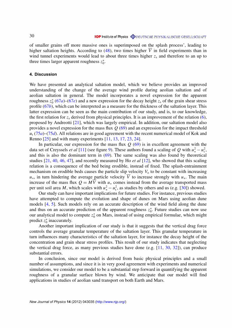
30

of smaller grains off more massive ones is superimposed on the splash process’, leading tohigher saltation heights. According to (48), two times higher V in field experiments than inwind tunnel experiments would lead to about three times higher zs and therefore to an up tothree times larger apparent roughness z∗

0.

4. Discussion

We have presented an analytical saltation model, which we believe provides an improvedunderstanding of the change of the average wind profile during aeolian saltation and ofaeolian saltation in general. The model incorporates a novel expression for the apparentroughness z∗

0 (67a)–(67e) and a new expression for the decay height zs of the grain shear stressprofile (67b), which can be interpreted as a measure for the thickness of the saltation layer. Thislatter expression can be seen as the main contribution of our study, and is, to our knowledge,the first relation for zs derived from physical principles. It is an improvement of the relation (6),proposed by Andreotti [21], which was largely empirical. In addition, our saltation model alsoprovides a novel expression for the mass flux Q (69) and an expression for the impact thresholdut (75a)–(75d). All relations are in good agreement with the recent numerical model of Kok andRenno [25] and with many experiments [11, 13, 17, 23, 24].

In particular, our expression for the mass flux Q (69) is in excellent agreement with thedata set of Creyssels et al [11] (see figure 9). These authors found a scaling of Q with u2

∗− u2

t ,and this is also the dominant term in (69). The same scaling was also found by theoreticalstudies [21, 40, 46, 47], and recently measured by Ho et al [12], who showed that this scalingrelation is a consequence of the bed being erodible, instead of fixed. The splash-entrainmentmechanism on erodible beds causes the particle slip velocity Vo to be constant with increasingu∗, in turn hindering the average particle velocity V to increase strongly with u∗. The mainincrease of the mass flux Q = MV with u∗ comes instead from the average transported massper unit soil area M , which scales with u2

∗− u2

t , as studies by others and us (e.g. [30]) showed.Our study can have important implications for future studies. For instance, previous studies

have attempted to compute the evolution and shape of dunes on Mars using aeolian dunemodels [4, 5]. Such models rely on an accurate description of the wind field along the duneand thus on an accurate prediction of the apparent roughness z∗

0. Future studies can now useour analytical model to compute z∗

0 on Mars, instead of using empirical formulae, which mightpredict z∗

0 inaccurately.Another important implication of our study is that it suggests that the vertical drag force

controls the average granular temperature of the saltation layer. This granular temperature inturn influences many characteristics of the saltation layer, for instance the decay height of theconcentration and grain shear stress profiles. This result of our study indicates that neglectingthe vertical drag force, as many previous studies have done (e.g. [11, 30, 32]), can producesubstantial errors.

In conclusion, since our model is derived from basic physical principles and a smallnumber of assumptions, and since it is in very good agreement with experiments and numericalsimulations, we consider our model to be a substantial step forward in quantifying the apparentroughness of a granular surface blown by wind. We anticipate that our model will findapplications in studies of aeolian sand transport on both Earth and Mars.


http://www.njp.org/

31

Acknowledgments

We acknowledge support from ETH grant ETH-10 09-2 and NFS grant AGS 1137716. We alsoacknowledge fruitful discussions with Dirk Kadau, Mathias Fuhr and Beat Luthi. We sincerelythank the two anonymous referees for many useful comments.

Appendix A. Supplementary information

This appendix contains information about our analytical model which deviates from the mainnarrative. First, we show how our model would change if we considered vertical drag in theforce balance. This is interesting since the result suggests that the slight change of α with theconditions we found in the numerical simulations of Kok and Renno [25] (see table 1) might belinked to vertical drag. Afterwards, we simplify our mass flux relation (69) to an explicit formwhich can be of use for further studies. Finally, we apply our model to calculate the impactthreshold ut on Mars as a function of d and show that our model predicts an impact thresholdwell below the fluid entrainment threshold on Mars.

A.1. The effect of vertical drag in the force balance

In the main paper, we neglected the effect of vertical drag in the force balance. Here, we discusshow the model would change if we considered it. Including vertical drag, fz can be written as

fz = −ρ g −3

4sd

(ρ↑Cd(vr↑)vr↑vz↑ + ρ↓Cd(vr↓)vr↓vz↓

), (A.1)

where we have used vrz↑(↓) = −vz↑(↓) and (26). Unlike what was done before, we cannotsimply integrate (A.1) over height and equalize the average of the function to the function ofaverages times a correlation factor, since this procedure is only accurate if all quantities havethe same sign, but here vz↓ is negative. However, an analytical treatment is possible if usingtwo approximations. Firstly, we approximate vr↑(↓) ≈ vrx↑(↓) similar to what was done before.Secondly, we assume the following functional form for the drag law:

Cd(V ) =Coµ

Vρwd+ C∞, (A.2)

where Co and C∞ = Cd(∞) are dimensionless parameters. Many drag laws in the literature aregiven in this form, e.g. [48, 49]. Also drag laws that differ from (A.2), e.g. [44], should at leastfollow it approximately. Using these approximations and (14), we can rewrite fz as

fz = −ρ g −3φ

4sd

(Cd(vrx↑)vrx↑ − Cd(vrx↓)vrx↓

)= −ρ g −

3C∞τg

4sd, (A.3)

where we further used (16) and Cd(vrx↑)vrx↑ − Cd(vrx↓)vrx↓ = C∞1vx . Using (19), heightintegration now yields

pgo = −gM −3C∞τgozs

4sd. (A.4)

Using this expression and performing the same analysis as in section 2.3 yields exactly the sameexpressions (32) and (34) if α is replaced by

α = α −3C∞zs

4sd. (A.5)


http://www.njp.org/

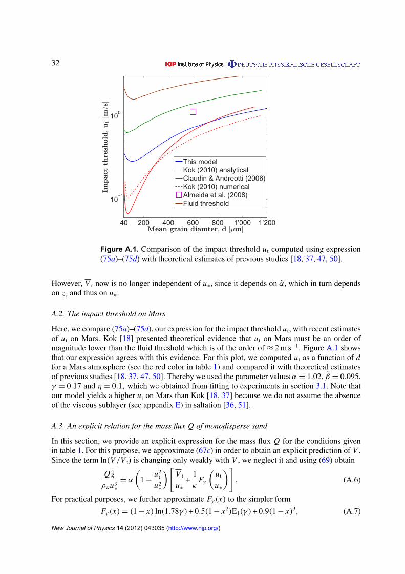
32

40 200 400 600 800 1’000 1’200

10−1

100

Mean grain diamter, d [µm]

Impactthreshold,ut[m/s]

This modelKok (2010) analyticalClaudin & Andreotti (2006)Kok (2010) numericalAlmeida et al. (2008)Fluid threshold

Figure A.1. Comparison of the impact threshold ut computed using expression(75a)–(75d) with theoretical estimates of previous studies [18, 37, 47, 50].

However, V r now is no longer independent of u∗, since it depends on α, which in turn dependson zs and thus on u∗.

A.2. The impact threshold on Mars

Here, we compare (75a)–(75d), our expression for the impact threshold ut, with recent estimatesof ut on Mars. Kok [18] presented theoretical evidence that ut on Mars must be an order ofmagnitude lower than the fluid threshold which is of the order of ≈ 2 m s−1. Figure A.1 showsthat our expression agrees with this evidence. For this plot, we computed ut as a function of dfor a Mars atmosphere (see the red color in table 1) and compared it with theoretical estimatesof previous studies [18, 37, 47, 50]. Thereby we used the parameter values α = 1.02, β = 0.095,γ = 0.17 and η = 0.1, which we obtained from fitting to experiments in section 3.1. Note thatour model yields a higher ut on Mars than Kok [18, 37] because we do not assume the absenceof the viscous sublayer (see appendix E) in saltation [36, 51].

A.3. An explicit relation for the mass flux Q of monodisperse sand

In this section, we provide an explicit expression for the mass flux Q for the conditions givenin table 1. For this purpose, we approximate (67c) in order to obtain an explicit prediction of V .Since the term ln(V /V t) is changing only weakly with V , we neglect it and using (69) obtain

Qg

ρwu3∗

= α

(1 −

u2t

u2∗

)[V t

u∗

+1

κFγ

(ut

u∗

)]. (A.6)

For practical purposes, we further approximate Fγ (x) to the simpler form

Fγ (x) = (1 − x) ln(1.78γ ) + 0.5(1 − x2)E1(γ ) + 0.9(1 − x)3, (A.7)


http://www.njp.org/

33

0 2 4 6 80

2

4

6

8

(1− ut/u∗)ln[3.5(sgd)0.5(μ/(ρwg2))1/3/zo]

ln(z∗sim

o/z o)

0 2 4 6 80

2

4

6

8

(1− ut/u∗)ln[40ut(μ/(ρwg2))1/3/zo]

ln(z∗sim

0/z o)

(a) (b)

Figure B.1. (a) ln(z∗

0/z0) calculated using the scaling law of Andreotti [21] (4)and (6) versus ln(z∗sim

0 /z0), the value of ln(z∗

0/z0) obtained directly from thesimulations. (b) The same as (a) but here

√sgd in (6) is replaced by ut. Thereby

the prefactors are chosen to ensure the best agreement with the blue condition intable 1 (blue circles). The same prefactor leads to very strong disagreement withthe red conditions in table 1. The values of ut, ρs, ρw, g, d , µ and z0 are takenfrom table 1. Each circle belongs to a different shear velocity u∗ with a differentln(z∗sim

0 /z0). The solid line indicates perfect agreement.

where we used (66) and the simpler approximation (D.21). With the values of α, γ , ut, and V t

given in table 1, one can explicitly calculate Q with (A.6) for free field conditions in differentenvironments. For instance, for Earth conditions with d = 250 µm (the third row in table 1), wecan write

Qg

ρwu3∗

=

(1 −

u2t

u2∗

)[2.1 m s−1

u∗

+

(1 −

u2t

u2∗

)+ 2.1

(1 −

ut

u∗

)3

− 1.4(u∗ − ut)

], (A.8)

where ut = 0.196 m s−1.

Appendix B. Comparison between the scaling law of Andreotti and the numerical data

In this appendix, we show that we failed to fit the numerical data for the apparent roughnessz∗

0 when using (6), the scaling for zs proposed by Andreotti [21]. Earth and Mars conditions(blue and red conditions in table 1) could not be fitted simultaneously by (4) and (6), oralternatively (67a) and (6) with a single proportionality constant in (6). Fitting to goodagreement with the numerical Earth data, led to a disagreement with the Mars data by almosttwo orders of magnitude, even after trying several modifications such as, for instance, replacing√

sgd in (6) by ut (see figure B.1). This indicates that (6) does not describe the physicssufficiently well. Andreotti [21] mentioned that (6) is an educated guess: ‘We have not found anysimple explanation of this scaling with ν = µ/ρw. The only indication that we have identifiedthe good parameter is the prefactor of order unity’.


http://www.njp.org/

34

Appendix C. Computing impact and lift-off velocities with the model of Kok

Kok [37] has recently derived analytic expressions for the average impact and lift-off velocities,from which we obtain the following expressions for the constants α and β and for the particleslip velocity Vo. They write

α =−1vzo

1vxo=

sin θivi + sin θlvl

cos θivi − cos θlvl, (C.1)

β =−1v2

zo

1v2xo

=(sin θivi)

2− (sin θlvl)

2

(cos θivi)2 − (cos θlvl)2, (C.2)

Vo =ρo↑vxo↑ + ρo↓vxo↓

ρo↑ + ρo↓

=sin θivi cos θlvl + sin θlvl cos θivi

sin θivi + sin θlvl, (C.3)

where θi ≈ 11◦, θl ≈ 40◦ and ρo↑vzo↑ + ρo↓vzo↓ = 0 were used (see (14)). vi and vl are furthergiven by

vi =1 − F

2r

√g f d −

1

2ε+

√1

4ε2+

(1 − F

2r

)2

g f d +1 + F

2rε

√g f d (C.4)

and

vl = FαRvi

(1 −

1

(1 + εvi)2

)+ αejvi

(1 − exp

(−

vi

40√

g f d

)), (C.5)

where the parameters are given by r = 0.02, F = 0.96, ε ≈ 1s/m, αR = 0.55, αej = 0.15√

g/g f

and g f is an effective gravity which incorporates the effect of cohesion at small particlediameters d ,

g f = g +6ζ

πρsd2. (C.6)

Here ζ is the dimensional cohesion parameter. Equation (C.6) expresses that cohesive forcesscale with d1, in contrast to the gravity force which scales with d3. This means that at small dcohesive forces become dominant. Shao and Lu [43] estimated that the magnitude of ζ rangesfrom about 1 × 10−4 N m−1 to 5 × 10−4 N m−1; we use ζ = 5 × 10−4 N m−1.

Appendix D. Calculation of the average wind velocity profile and the apparent roughness

In this appendix, we show how one can compute the average wind velocity profile and theapparent roughness from an exponentially decaying grain shear stress profile,

τg(z) = τgo e−z/zs . (D.1)

The average wind velocity profile u(z) can be obtained from Prandtl’s mixing lengthapproximation [19, 20, 22, 30, 33] as

du(z)

dz=

ua(z)

κz=

u∗

κz

√1 − τg(z)/τ (D.2)

with the boundary condition

u(z0) = 0. (D.3)


http://www.njp.org/

35

The apparent roughness z∗

0 is the roughness of the asymptotic fluid velocity profile v(z) =

v(z)|z→∞, giving

u(z) =u∗

κln

z

z∗

0

. (D.4)

In order to integrate (D.2) analytically, we Taylor-expand the square root in (D.2) in theargument a exp(−z/zs), where a = τgo/τ . The square root becomes

√1 − x = 1 −

∞∑j=1

f j xj , (D.5)

where f j is given by

f j =(2 j − 3)!!

(2 j)!!. (D.6)

Then (D.2) becomes

u(z) =u∗

κ

lnz

z0−

∞∑j=1

f jaj

∫ z

z0

dz′

z′e− j z′/zs

. (D.7)

Within the integral we transform the z-coordinate using

x =j z′

zs, (D.8)

such that the integral transforms to∫ z

z0

dz′

z′e− j z′/zs =

∫ j z/zs

j z0/zs

dx

xe−x

= E1( j z0/zs) − E1( j z/zs), (D.9)

where E1(x) is called the exponential integral. It can be expressed as

E1(x) = −0.577 − ln x + Ein(x), (D.10)

where 0.577 is the Euler–Mascheroni constant,

0.57721 . . . = limn→∞

(n∑

k=1

1

k− ln(n)

), (D.11)

and Ein(x) is an analytic function with the series-expansion

Ein(x) =

∞∑l=1

(−1)l+1x l

ll!. (D.12)

E1(x) vanishes for x → ∞. Using (D.9), the velocity profile can finally be written as

u(z) =u∗

κ

lnz

z0−

∞∑j=1

f jaj (E1( j z0/zs) − E1( j z/zs))

. (D.13)


http://www.njp.org/

36

A comparison with the asymptotic profile (D.4) then yields

lnz∗

0

z0=

∞∑j=1

f jaj E1( j z0/zs). (D.14)

Since z0 � zs, (D.14) can further be written as

lnz∗

0

z0= −K (a) + (1 −

√1 − a)

(ln

zs

z0− 0.577

), (D.15)

where K (a) is defined by

K (a) =

∞∑j=2

f j ln( j)a j . (D.16)

To our knowledge, the sum on the right-hand side is not analytically treatable with commonmethods. However, we found that it can be very well approximated by

K (a)u 1.154(1 −√

1 − a)2.56(1 +√

1 − a ln√

1 − a), (D.17)

where both constants, 2.56 and 1.154, are fit constants ensuring very good agreement betweenthe infinite sum and the approximation. This approximation performs very well over the wholerange of a, the relative errors being typically below 1%. A simpler but worse approximation isgiven by

K (a)u 0.9(1 −√

1 − a)3. (D.18)

Both approximations are shown in figure D.1. Using (D.17) we can finally write

lnz∗

0

z0=

(1 −

ub

u∗

)ln

zs

1.78z0+ G

(ub

u∗

), (D.19)

where ub = u∗

√1 − a was used (see (57)), 1.78 = exp(0.577) and G(x) is defined by

G(x) = 1.154(1 + x ln x)(1 − x)2.56. (D.20)

If we used the simpler approximation (D.18) instead of (D.17), G(x) would write

G(x) = 0.9(1 − x)3. (D.21)

D.1. Approximation for large z

Now we further calculate an approximative expression for the wind profile at large heights z.The velocity profile in (D.13) can be rewritten as

u(z) =u∗

κ

lnz

z∗

0

+∞∑j=1

f jaj E1( j z/zs)

, (D.22)


http://www.njp.org/

37

0 0.2 0.4 0.6 0.8 10

0.2

0.4

0.6

0.8

1

a

K(a)

Figure D.1. Comparison between K (a) computed using (D.16) with an accuracyof at least 10−5 (squares) and K (a) computed with the approximations (D.17)(solid line) and (D.18) (dashed line) for 06 a 6 0.999.

where we inserted (D.14). If z/zs is large enough, it is sufficient to only consider the first termof the Taylor expansion because E1(x) decreases strongly with increasing argument x . Thiseventually yields

u(z) =u∗

κln

z

z∗

0

+u2

∗− u2

b

2κu∗

E1

(z

zs

), (D.23)

where we also inserted (57) and (D.19).

D.2. Approximation for z < zs

Here we motivate an approximation of the wind profile u(z) for small heights z < zs. For thispurpose, we first make an approximation for the infinite sum

I

(a,

z

zs

)=

∞∑j=1

f jaj Ein( j z/zs), (D.24)

and then insert it into the velocity profile, given by (D.22). Inserting the series expansion (D.12)of Ein in (D.24) and exchanging the order of the sums gives

I =

∞∑k=1

∞∑j=1

f jaj (−1)k+1 j k(z/zs)

k

kk!. (D.25)

The inner sum can be written as∞∑j=1

f jaj j k

= (a∂a)k[1 −

√1 − a].


http://www.njp.org/

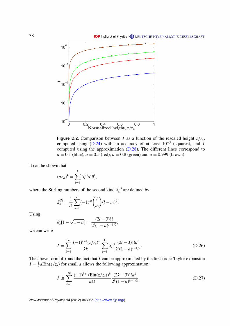
38

0 0.2 0.4 0.6 0.8 110

−4

10−3

10−2

10−1

100

Normalized height, z/zs

I

Figure D.2. Comparison between I as a function of the rescaled height z/zs,computed using (D.24) with an accuracy of at least 10−5 (squares), and Icomputed using the approximation (D.28). The different lines correspond toa = 0.1 (blue), a = 0.5 (red), a = 0.8 (green) and a = 0.999 (brown).

It can be shown that

(a∂a)k=

k∑l=1

S(l)k al∂ l

a,

where the Stirling numbers of the second kind S(l)k are defined by

S(l)k =

1

l!

l∑m=0

(−1)m

(l

m

)(l − m)k.

Using

∂ la[1 −

√1 − a] =

(2l − 3)!!

2l(1 − a)l−1/2,

we can write

I =

∞∑k=1

(−1)k+1(z/zs)k

kk!

k∑l=1

S(l)k

(2l − 3)!!al

2l(1 − a)l−1/2. (D.26)

The above form of I and the fact that I can be approximated by the first-order Taylor expansionI =

12aEin(z/zs) for small a allows the following approximation:

I u∞∑

k=1

(−1)k+1(Ein(z/zs))k

kk!

(2k − 3)!!ak

2k(1 − a)k−1/2, (D.27)


http://www.njp.org/

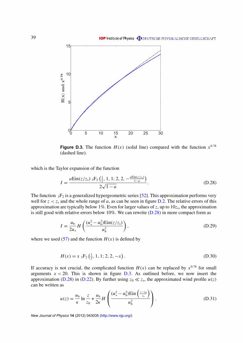
39

0 5 10 15 20 25 300

5

10

15

x

H(x)andx0.78

Figure D.3. The function H(x) (solid line) compared with the function x0.78

(dashed line).

which is the Taylor expansion of the function

I =aEin(z/zs) 3F2

(12 , 1, 1; 2, 2, −

aEin(z/zs)

1−a

)2√

1 − a. (D.28)

The function 3F2 is a generalized hypergeometric series [52]. This approximation performs verywell for z < zs and the whole range of a, as can be seen in figure D.2. The relative errors of thisapproximation are typically below 1%. Even for larger values of z, up to 10zs, the approximationis still good with relative errors below 10%. We can rewrite (D.28) in more compact form as

I =ub

2u∗

H

((u2

∗− u2

b)Ein(z/zs)

u2b

), (D.29)

where we used (57) and the function H(x) is defined by

H(x) = x 3F2

(12 , 1, 1; 2, 2, −x

). (D.30)

If accuracy is not crucial, the complicated function H(x) can be replaced by x0.78 for smallarguments x < 20. This is shown in figure D.3. As outlined before, we now insert theapproximation (D.28) in (D.22). By further using z0 � zs, the approximated wind profile u(z)can be written as

u(z) =ub

κln

z

z0+

ub

2κH

(u2∗− u2

b)Ein(

z−z0zs

)u2

b

. (D.31)


http://www.njp.org/

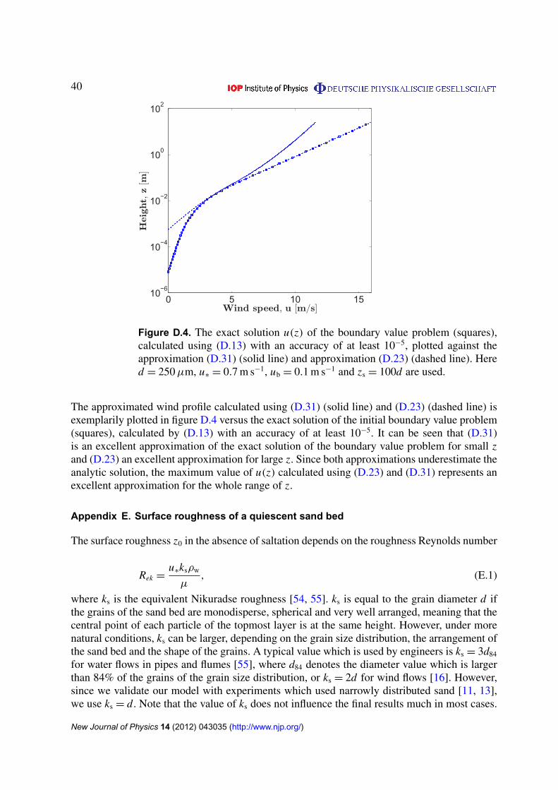
40

0 5 10 1510

−6

10−4

10−2

100

102

Wind speed, u [m/s]

Height,z[m]

Figure D.4. The exact solution u(z) of the boundary value problem (squares),calculated using (D.13) with an accuracy of at least 10−5, plotted against theapproximation (D.31) (solid line) and approximation (D.23) (dashed line). Hered = 250 µm, u∗ = 0.7 m s−1, ub = 0.1 m s−1 and zs = 100d are used.

The approximated wind profile calculated using (D.31) (solid line) and (D.23) (dashed line) isexemplarily plotted in figure D.4 versus the exact solution of the initial boundary value problem(squares), calculated by (D.13) with an accuracy of at least 10−5. It can be seen that (D.31)is an excellent approximation of the exact solution of the boundary value problem for small zand (D.23) an excellent approximation for large z. Since both approximations underestimate theanalytic solution, the maximum value of u(z) calculated using (D.23) and (D.31) represents anexcellent approximation for the whole range of z.

Appendix E. Surface roughness of a quiescent sand bed

The surface roughness z0 in the absence of saltation depends on the roughness Reynolds number

Rek =u∗ksρw

µ, (E.1)

where ks is the equivalent Nikuradse roughness [54, 55]. ks is equal to the grain diameter d ifthe grains of the sand bed are monodisperse, spherical and very well arranged, meaning that thecentral point of each particle of the topmost layer is at the same height. However, under morenatural conditions, ks can be larger, depending on the grain size distribution, the arrangement ofthe sand bed and the shape of the grains. A typical value which is used by engineers is ks = 3d84

for water flows in pipes and flumes [55], where d84 denotes the diameter value which is largerthan 84% of the grains of the grain size distribution, or ks = 2d for wind flows [16]. However,since we validate our model with experiments which used narrowly distributed sand [11, 13],we use ks = d. Note that the value of ks does not influence the final results much in most cases.


http://www.njp.org/

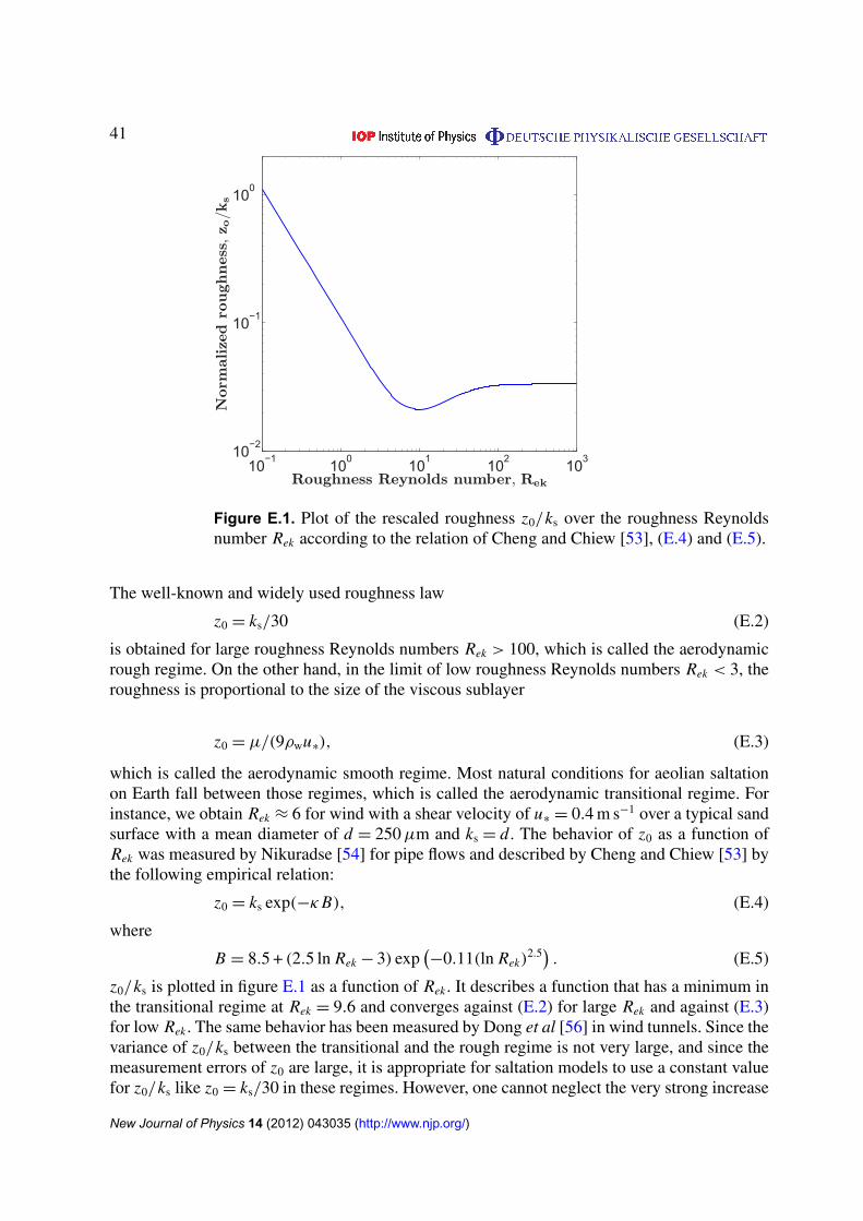
41

10−1

100

101

102

10310

−2

10−1

100

Roughness Reynolds number, Rek

Normalizedroughness,z o/ks

Figure E.1. Plot of the rescaled roughness z0/ks over the roughness Reynoldsnumber Rek according to the relation of Cheng and Chiew [53], (E.4) and (E.5).

The well-known and widely used roughness law

z0 = ks/30 (E.2)

is obtained for large roughness Reynolds numbers Rek > 100, which is called the aerodynamicrough regime. On the other hand, in the limit of low roughness Reynolds numbers Rek < 3, theroughness is proportional to the size of the viscous sublayer

z0 = µ/(9ρwu∗), (E.3)

which is called the aerodynamic smooth regime. Most natural conditions for aeolian saltationon Earth fall between those regimes, which is called the aerodynamic transitional regime. Forinstance, we obtain Rek ≈ 6 for wind with a shear velocity of u∗ = 0.4 m s−1 over a typical sandsurface with a mean diameter of d = 250 µm and ks = d. The behavior of z0 as a function ofRek was measured by Nikuradse [54] for pipe flows and described by Cheng and Chiew [53] bythe following empirical relation:

z0 = ks exp(−κ B), (E.4)

where

B = 8.5 + (2.5 ln Rek − 3) exp(−0.11(ln Rek)

2.5). (E.5)

z0/ks is plotted in figure E.1 as a function of Rek . It describes a function that has a minimum inthe transitional regime at Rek = 9.6 and converges against (E.2) for large Rek and against (E.3)for low Rek . The same behavior has been measured by Dong et al [56] in wind tunnels. Since thevariance of z0/ks between the transitional and the rough regime is not very large, and since themeasurement errors of z0 are large, it is appropriate for saltation models to use a constant valuefor z0/ks like z0 = ks/30 in these regimes. However, one cannot neglect the very strong increase


http://www.njp.org/

42

of z0 for Reynolds numbers below Rek = 3 in the smooth regime. Since we consider very smallparticle diameters in our model, for which Rek < 3, we use (E.4) and (E.5) to compute z0.

References

[1] Bagnold R A 1941 The Physics of Blown Sand and Desert Dunes (New York: Methuen)[2] Kroy K, Sauermann G and Herrmann H J 2002 Minimal model for aeolian sand dunes Phys. Rev. E 66 031302[3] Kroy K, Sauermann G and Herrmann H J 2002 A minimal model for sand dunes Phys. Rev. Lett. 64 054301[4] Parteli E J R and Herrmann H J 2007 Dune formation on the present Mars Phys. Rev. E 76 041307[5] Parteli E J R and Herrmann H J 2007 Saltation transport on Mars Phys. Rev. Lett. 98 198001[6] Parteli E J R, Duran O and Herrmann H J 2007 Minimal size of a barchan dune Phys. Rev. E 75 011301[7] Owen P R 1964 Saltation of uniform grains in air J. Fluid Mech. 20 225–42[8] Charnock H 1955 Wind stress on a water surface Q. J. R. Meteorol. Soc. 81 639–40[9] Namikas S L 2003 Field measurement and numerical modelling of aeolian mass flux distributions on a sandy

beach Sedimentology 50 303–26[10] Rasmussen K R and Sorensen M 2008 Vertical variation of particle speed and flux density in aeolian saltation:

measurement and modeling J. Geophys. Res. 113 F02S12[11] Creysells M, Dupont P, Ould el Moctar A, Valance A, Cantat I, Jenkins J T, Pasini J M and Rasmussen K R

2009 Saltating particles in a turbulent boundary layer: experiment and theory J. Fluid Mech. 625 47–74[12] Ho T D, Valance A, Dupont P and Ould El Moctar A 2011 Scaling laws in aeolian sand transport Phys. Rev.

Lett. 106 094501[13] Rasmussen K R, Iversen J D and Rautahemio P 1996 Saltation and wind-flow interaction in a variable slope

wind tunnel Geomorphology 17 19–28[14] Dong Z, Liu X and Wang H 2003 The aerodynamic roughness with a blowing sand boundary layer (bsbl): a

redefinition of the Owen effect Geophys. Res. Lett. 30 1047[15] Sherman D J and Farrell E J 2008 Aerodynamic roughness lengths over movable beds: comparison of wind

tunnel and field data J. Geophys. Res. 113 F02S08[16] Sherman D J 1992 An equilibrium relationship for shear velocity and roughness length in aeolian saltation

Geomorphology 5 419–31[17] Bagnold R A 1937 The transport of sand by wind Geogr. J. 89 409–38[18] Kok J F 2010 Difference in the wind speeds required for initiation versus continuation of sand transport on

Mars: implications for dunes and dust storms Phys. Rev. Lett. 104 074502[19] Raupach M R 1991 Saltation layers, vegetation canopies and roughness lengths Acta Mech. Suppl. 1 83–96[20] Prandtl L 1925 Uber die ausgebildete turbulenz Z. Angew. Math. Mech. 5 136–9[21] Andreotti B 2004 A two-species model of aeolian sand transport J. Fluid Mech. 510 47–70[22] Duran O and Herrmann H J 2006 Modelling of saturated sand flux J. Stat. Mech. P07011[23] Chepil W S 1945 Dynamics of wind erosion: II. Initiation of soil movement Soil Sci. 60 397–411[24] Rasmussen K R, Iversen J D and Rautahemio P 1994 The effect of surface slope on saltation threshold

Sedimentology 41 721–8[25] Kok J F and Renno N O 2009 A comprehensive numerical model of steady state saltation (comsalt)

J. Geophys. Res. 114 D17204[26] Sorensen M and McEwan I 1996 On the effect of mid-air collisions on aeolian saltation Sedimentology

43 65–76[27] Dong Z, Huang N and Liu X 2005 Simulation of the probability of midair interparticle collisions in an aeolian

saltating cloud J. Geophys. Res. 110 D24113[28] Huang N, Zhang Y and D’Adomo R 2007 A model of the trajectories and midair collision probabilities of

sand particles in a steady state saltation cloud J. Geophys. Res. 112 D08206[29] Ren S and Huang N 2010 A numerical model of the evolution of sand saltation with consideration of two

feedback mechanisms Eur. Phys. J. E 33 351–8


http://dx.doi.org/10.1103/PhysRevE.66.031302

http://dx.doi.org/10.1103/PhysRevLett.88.054301




http://dx.doi.org/10.1017/S0022112064001173

http://dx.doi.org/10.1002/(ISSN)1477-870X

http://dx.doi.org/10.1046/j.1365-3091.2003.00556.x

http://dx.doi.org/10.1029/2007JF000774

http://dx.doi.org/10.1017/S0022112008005491


http://dx.doi.org/10.1016/0169-555X(95)00090-R

http://dx.doi.org/10.1029/2002GL016318

http://dx.doi.org/10.1029/2007JF000784

http://dx.doi.org/10.1016/0169-555X(92)90016-H

http://dx.doi.org/10.2307/1786411


http://dx.doi.org/10.1007/978-3-7091-6706-9

http://dx.doi.org/10.1017/S0022112004009073

http://dx.doi.org/10.1088/1742-5468/2006/07/P07011

http://dx.doi.org/10.1097/00010694-194511000-00005

http://dx.doi.org/10.1111/sed.1994.41.issue-4

http://dx.doi.org/10.1029/2009JD011702


http://dx.doi.org/10.1029/2005JD006070

http://dx.doi.org/10.1029/2006JD007480

http://dx.doi.org/10.1140/epje/i2010-10681-4

http://www.njp.org/

43

[30] Sauermann G, Kroy K and Herrmann H J 2001 A continuum saltation model for sand dunes Phys. Rev. E64 31305

[31] Van Rijn L C 1984 Sediment transport. Part I: bed load transport J. Hydraul. Eng. 110 1431–56[32] Jenkins J T, Cantat I and Valance A 2010 Continuum model for steady, fully developed saltation above a

horizontal particle bed Phys. Rev. E 82 020301[33] Anderson R S and Haff P K 1991 Wind modification and bed response during saltation of sand in air Acta

Mech. Suppl. 1 21–51[34] Leal L G 2007 Advanced Transport Phenomena: Fluid Mechanics and Convective Transport Processes

(Cambridge: Cambridge University Press)[35] Bagnold R A 1973 The nature of saltation and ‘bed-load’ transport in water Proc. R. Soc. A 332 473–504[36] Kok J F, Parteli E J R, Michaels T I and Karam D B 2012 The physics of wind-blown sand and dust

arXiv:1201.4353[37] Kok J F 2010 An improved parameterization of wind blown sand flux on Mars that includes the effect of

hysteresis Geophys. Res. Lett. 37 L12202[38] Oger L, Ammi M, Valance A and Beladjine D 2008 Study of the collision of one rapid sphere on 3d packings:

experimental and numerical results Comput. Math. Appl. 55 132–48[39] Anderson R S and Hallet B 1986 Sediment transport by wind: toward a general model Geol. Soc. Am. Bull.

97 523–35[40] Ungar J E and Haff P K 1987 Steady state saltation in air Sedimentology 34 289–99[41] Bagnold R A 1938 The measurement of sand storms Proc. R. Soc. A 167 282–91[42] Sorensen M 1996 An analytic model of wind-blown sand transport Acta Mech. Suppl. 1 67–81[43] Shao Y and Lu H 2000 A simple expression for wind erosion threshold friction velocity J. Geophys. Res.

105 22437–43[44] Cheng N S 1997 Simplified settling velocity formula for sediment particle J. Hydraul. Eng. 123 149–52[45] Iversen J D and Rasmussen K R 1999 The effect of wind speed and bed slope on sand transport Sedimentology

46 723–31[46] Almeida M P, Andrade J S and Herrmann H J 2007 Aeolian transport of sand Eur. Phys. J. E 22 195–200[47] Almeida M P, Parteli E J R, Andrade J S and Herrmann H J 2008 Giant saltation on Mars Proc. Natl Acad.

Sci. 105 6222–6[48] Rubey W W 1933 Settling velocity of gravel, sand and silt particles Am. J. Sci. 5 325–38[49] Julien P Y 1995 Erosion and Sedimentation (Cambridge: Press Syndicate of the University of Cambridge)[50] Claudin P and Andreotti B 2006 A scaling law for aeolian dunes on mars, venus, earth, and for subaqueous

ripples Earth Planet. Sci. Lett. 252 30–44[51] White B R 1979 Soil transport by winds on Mars J. Geophys. Res. 84 4643–51[52] National Institute of Standards and Technology 2012 Digital Library of Mathematical Functions chapter 16

(http://dlmf.nist.gov/16)[53] Cheng N S and Chiew Y M 1998 Modified logarithmic law for velocity distribution subjected to upward

seepage J. Hydraul. Eng. 124 1235–41[54] Nikuradse J 1933 Stromungsgesetze in rauhen Rohren Forschungsheft 361, Teil B (Berlin: VDI Verlag)

Nikuradse J 1950 Laws of flow in rough pipes NACA TM 1292 (Engl. transl.)[55] Keulegan G H 1938 Laws of turbulent flow in open channels J. Natl Bur. Stand. 21 707–41 (Research Paper

1151)[56] Dong Z, Wang X, Zhao A, Liu L and Liu X 2001 Aerodynamic roughness of fixed sand beds J. Geophys.

Res. 106 11001–11



http://dx.doi.org/10.1061/(ASCE)0733-9429(1984)110:10(1431)


http://dx.doi.org/10.1007/978-3-7091-6706-9

http://dx.doi.org/10.1098/rspa.1973.0038

http://arxiv.org/abs/1201.4353

http://dx.doi.org/10.1029/2010GL043646

http://dx.doi.org/10.1016/j.camwa.2007.04.001

http://dx.doi.org/10.1130/0016-7606(1986)97< 523:STBWTA> 2.0.CO;2


http://dx.doi.org/10.1098/rspa.1938.0132

http://dx.doi.org/10.1007/978-3-7091-6706-9

http://dx.doi.org/10.1029/2000JD900304


http://dx.doi.org/10.1046/j.1365-3091.1999.00245.x

http://dx.doi.org/10.1140/epje/e2007-00028-7

http://dx.doi.org/10.1073/pnas.0800202105

http://dx.doi.org/10.2475/ajs.s5-25.148.325

http://dx.doi.org/10.1016/j.epsl.2006.09.004

http://dx.doi.org/10.1029/JB084iB09p04643

http://dlmf.nist.gov/16


http://dx.doi.org/10.1029/2001JB900009

http://www.njp.org/

the apparent roughness of a sand surface blown by wind ... · pdf filethe open access journal...

Documents