the antarctic atmospheric energy budget. part ii:...

The Antarctic Atmospheric Energy Budget. Part II: The Effect of Ozone Depletionand its Projected Recovery

KAREN L. SMITH AND MICHAEL PREVIDI

Lamont-Doherty Earth Observatory, Palisades, New York

LORENZO M. POLVANI

Department of Applied Physics and Mathematics, Department of Earth and Environmental Sciences, Columbia University,

New York, New York

(Manuscript received 13 March 2013, in final form 12 June 2013)

ABSTRACT

In this study the authors continue their investigation of the atmospheric energy budget of the Antarctic

polar cap (the region poleward of 708S) using integrations of the Whole Atmosphere Community Climate

Model from the years 1960 to 2065. In agreement with observational data, it is found that the climatological

mean net top-of-atmosphere (TOA) radiative flux is primarily balanced by the horizontal energy flux con-

vergence over the polar cap. On interannual time scales, changes in the net TOA radiative flux are also

primarily balanced by changes in the energy flux convergence, with the variability in both terms significantly

correlated (positively and negatively, respectively) with the southern annular mode (SAM). Onmultidecadal

time scales, twentieth-century stratospheric ozone depletion produces a negative trend in the net TOA ra-

diative flux due to a decrease in the absorbed solar radiation within the atmosphere–surface column. The

negative trend in the net TOA radiative flux is balanced by a positive trend in energy flux convergence,

primarily in austral summer. This negative (positive) trend in the net TOA radiation (energy flux conver-

gence) occurs despite a positive trend in the SAM, suggesting that the effects of the SAM on the energy

budget are overwhelmed by the direct radiative effects of ozone depletion. In the twenty-first century, ozone

recovery is expected to reverse the negative trend in the net TOA radiative flux, which would then, again, be

balanced by a decrease in the energy flux convergence. Therefore, over the next several decades, ozone

recovery will, in all likelihood, mask the effect of greenhouse gas warming on the Antarctic energy budget.

1. Introduction

The dominant driver of recent multidecadal change

in the Antarctic climate system has been the depletion

of stratospheric ozone [see Thompson et al. (2011) for

a recent review]. The formation of the ozone hole over

the South Pole has been associated with a cooling of the

stratosphere and much of the Antarctic continent, a

warming of the Antarctic peninsula (Steig et al. 2009),

a poleward shift of the storm tracks (Polvani et al. 2011b;

Son et al. 2010, 2009; Lee and Feldstein 2013), a pole-

ward shift in subtropical precipitation (Kang et al. 2011),

and changes in Southern Ocean mixing and ventilation

(Sall�ee et al. 2010; Waugh et al. 2013). The changes in

the atmospheric circulation (i.e., lowered geopotential

heights over Antarctica and raised geopotential heights

over the southern midlatitudes, resulting in strength-

ened westerlies) are characteristic of the southern an-

nular mode (SAM), the dominant mode of Southern

Hemisphere extratropical circulation variability, which

has been experiencing a positive trend over the past

several decades. Despite the many studies examining

the role of ozone depletion in large-scale atmospheric

circulation trends, none has examined the implications

of ozone depletion for atmospheric energy transport

into the Antarctic polar cap.

Compared to the Arctic, the atmospheric energy

budget of the Antarctic has received relatively little

attention (Cullather and Bosilovich 2012; Genthon and

Krinner 1998; Nakamura and Oort 1988). Arctic climate

change, including dramatic sea ice loss and surface and

Corresponding author address: Karen L. Smith, Lamont-Doherty

Earth Observatory, 207B Oceanography, 61 Route 9W, P.O. Box

1000, Palisades, NY 10964.

E-mail: [email protected]

VOLUME 26 J OURNAL OF CL IMATE 15 DECEMBER 2013

DOI: 10.1175/JCLI-D-13-00173.1

� 2013 American Meteorological Society 9729

mailto:[email protected]

midtropospheric warming, has motivated numerous

studies of the energy budget in this region (Kay et al.

2012; Cullather and Bosilovich 2012; Porter et al. 2010;

Serreze et al. 2007; Nakamura and Oort 1988). Al-

though the Antarctic has not experienced comparable

polar amplification, the dramatic change in the top-of-

atmosphere (TOA) shortwave radiative flux associated

with SouthernHemisphere stratospheric ozone depletion

has likely had an important influence on the Antarctic

energy budget. In addition, the recovery of stratospheric

ozone in the future may influence the degree of Southern

Hemisphere polar amplification we can expect in the

coming decades.

In Part I, Previdi et al. (2013, hereafter Part I), we

examined the climatological mean and intraseasonal-

to-interannual variability of the components of the

Antarctic energy budget using reanalysis and satellite

data, and found a two-way balance between the net TOA

radiative flux and the horizontal energy flux convergence

over the polar cap. This two-way balance is reflected in

significant and opposite-signed correlations between

these terms and the SAM; the net TOA radiative flux is

positively correlated with the SAM while the energy flux

convergence is negatively correlated with the SAM. In

light of the positive trend in the SAM over the past few

decades, can one infer from interannual relationships that

net TOA flux has been increasing and the energy flux

convergence has been decreasing over this time period?

This question will be addressed in this study.

Although direct observation of the Antarctic climate

system over the past several decades has improved,

observation of the climate of the high southern latitudes

continues to be spatially and temporally limited; thus,

we need to rely on models and reanalyses to aid us in es-

timating and interpreting the changes that have occurred.

The lack of continuous observational data is a particular

hindrance for assessing the multidecadal effect of ozone

depletion on theAntarctic energy budget. First, there is no

record of the TOA radiative fluxes prior to the formation

of the ozone hole. Second, direct satellitemeasurements of

the TOA radiative fluxes in the period since consist of

short and discontinuous time series. The longest and most

recent record is the Clouds and the Earth’s Radiant En-

ergy System (CERES) dataset that began inMarch 2000.

However, during the period from 2000 to the present,

ozone levels in the Southern Hemisphere have leveled

off due to global regulations on chlorofluorocarbons

(CFCs; ScientificAssessment ofOzoneDepletion;WMO

2010), making this time period inappropriate for de-

tecting TOA trends due to ozone depletion.

The other satellite time series of TOAfluxes is from the

Earth Radiation Budget Experiment (ERBE), which ran

from February 1985 to April 1989. This is a short dataset

and it is difficult to directly compare it with CERES,

given that they are derived from different instruments

with their own biases. After some bias correction, Fasullo

andTrenberth (2008) show significant differences between

climatological ERBE and CERES net TOA shortwave

and longwave radiative fluxes at high southern latitudes

in austral spring, consistent with the effect of ozone de-

pletion (a decrease in both absorbed solar and outgoing

longwave radiation in CERES relative to ERBE; see

their Fig. 1). It is difficult to attribute these differences to

ozone, however, given that differences between the two

datasets are significant in many other parts of the globe

and at other times of the year (i.e., when ozone depletion

would be expected to be unimportant). Furthermore, the

CERES dataset includes the September 2002 strato-

spheric sudden warming, which has likely skewed the

springtime mean of the net TOA flux in CERES over

Antarctica given that sudden warmings in the Southern

Hemisphere are very rare (the September 2002 TOA

longwave flux anomaly averaged from 708 to 908S was

more than two standard deviations outside the 2001–10

CERES mean).

Reanalyses are extremely useful tools for investigating

the climate of the recent past; however, because of the

adverse effect of biases in observed ozone on the analysis,

reanalysis products do not assimilate time-varying ozone

data using analysis schemes that allow ozone to interact

with other dynamical fields (Dee et al. 2011). In addition,

reanalyses of the high-latitude Southern Hemisphere

prior to the satellite era are poorly constrained by obser-

vations and must be used with caution (Kistler et al. 2001).

To circumvent the issues with satellite and reanalysis

data, we investigate the extent to which ozone depletion

and projected recovery influence the Antarctic energy

budget using a fully coupled, state-of-the-art, stratosphere-

resolving model with interactive stratospheric chemistry.

In addition to investigating the trends in the Antarctic

energy budget in an ensemble of twentieth-century model

integrations, we also compare two ensembles of twenty-

first-century integrations, one with and one without ozone

recovery. We find that trends in the Antarctic energy

budget in the twentieth century are dominated by the ef-

fects of ozone depletion, particularly the TOA shortwave

radiative flux in spring and summer. In the future, ozone

recovery should reverse these trends.

2. Methods

a. Model

We employ the Community Earth System Model ver-

sion 1 (CESM1) using theWholeAtmosphereCommunity

Climate Model atmospheric component [CESM1

(WACCM); hereafter simply WACCM], that is, the

9730 JOURNAL OF CL IMATE VOLUME 26

stratosphere-resolving, coupled-chemistry version of the

National Center for Atmospheric Research (NCAR)

Community Atmosphere Model version 4 (CAM4) (Gent

et al. 2011). The land, ocean, and sea ice components of

WACCM are identical to those in CESM1. In contrast, the

WACCM atmospheric component has 66 vertical levels

with a model top at 140 km, a horizontal resolution of

1.98 3 2.58, special parameterizations for gravity waves

and other upper atmospheric processes, and, most im-

portantly, fully interactive stratospheric chemistry.

The WACCM twentieth-century ensemble comprises

three integrations and extends from 1960 to 2000 (labeled

20C). These integrations follow the Coupled Model

Intercomparison Project phase 5 (CMIP5) Historical

scenario for surface greenhouse gas concentrations

(Meinshausen et al. 2011). The Historical scenario also

includes prescribed surface concentrations of ozone-

depleting substances (ODSs). For further details on the

model and the twentieth-century integrations the reader

is referred to Marsh et al. (2013).

To examine the role of ozone recovery in the twenty-

first century we contrast two ensembles of model runs,

each comprising three integrations, from 2001 to 2065.

These model integrations were previously examined in

Smith et al. (2012) for Antarctic sea ice. For the first

ensemble (labeled 21C), forcings for the years 2001–05

are specified following the CMIP5 Historical scenario

and forcings for the years 2006–65 are specified follow-

ing representative concentration pathway 4.5 (RCP 4.5;

Meinshausen et al. 2011). The RCP 4.5 members are

initialized from the three corresponding Historical in-

tegrations described above (Marsh et al. 2013). For the

second twenty-first century ensemble (labeled FixODS),

everything is identical to 21C except for the surface

concentrations of ODSs, which are held fixed at year

2000 levels. In other words, we compare two future

scenarios in which greenhouse gas (GHG) concentra-

tions increase, but one includes ozone recovery (21C)

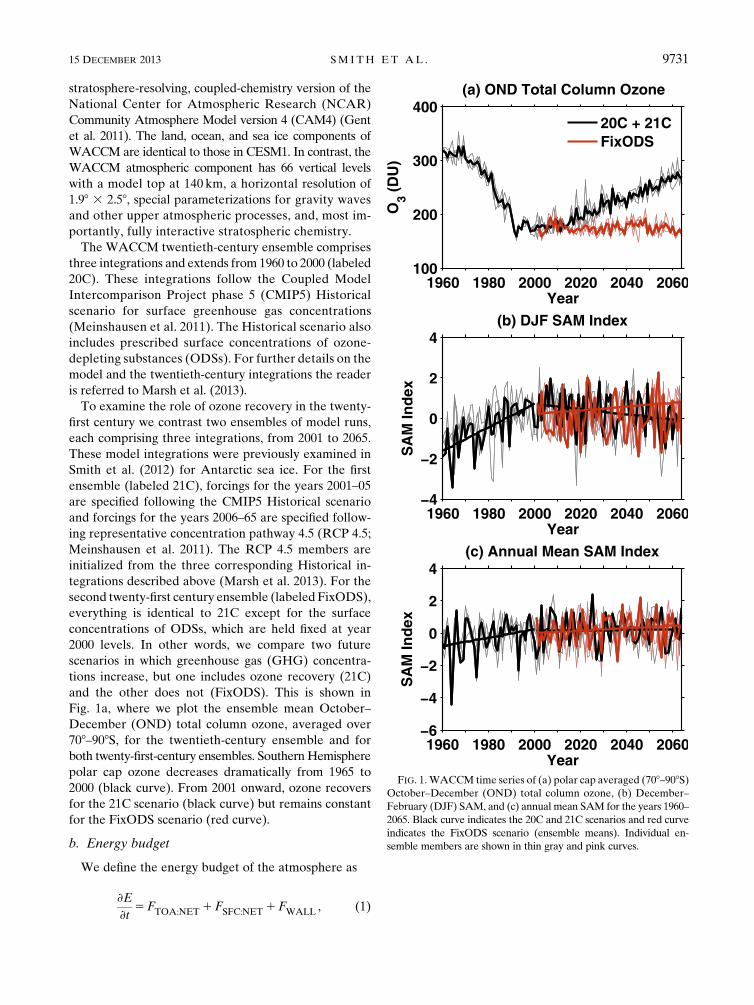
and the other does not (FixODS). This is shown in

Fig. 1a, where we plot the ensemble mean October–

December (OND) total column ozone, averaged over

708–908S, for the twentieth-century ensemble and for

both twenty-first-century ensembles. SouthernHemisphere

polar cap ozone decreases dramatically from 1965 to

2000 (black curve). From 2001 onward, ozone recovers

for the 21C scenario (black curve) but remains constant

for the FixODS scenario (red curve).

b. Energy budget

We define the energy budget of the atmosphere as

›E

›t5FTOA:NET1FSFC:NET 1FWALL , (1)

FIG. 1.WACCM time series of (a) polar cap averaged (708–908S)October–December (OND) total column ozone, (b) December–

February (DJF) SAM, and (c) annual mean SAM for the years 1960–

2065. Black curve indicates the 20C and 21C scenarios and red curve

indicates the FixODS scenario (ensemble means). Individual en-

semble members are shown in thin gray and pink curves.

15 DECEMBER 2013 SM I TH ET AL . 9731

where ›E/›t is the vertically integrated atmospheric

energy storage, FTOA:NET is the net top-of-atmosphere

(TOA) radiative flux, FSFC:NET is the net surface energy

flux (including radiative, sensible, and latent heat fluxes),

and FWALL is the vertically integrated horizontal en-

ergy flux convergence. The energy storage term can be

written as

›E

›t5

›

›t

ðps

0(cpT1Fs 1Lq1k)

dp

g, (2)

where g is the gravitational acceleration, p is pressure, ps is

the surface pressure, cp is the specific heat of air at constant

pressure, T is the absolute temperature, Fs is the surface

geopotential,L is the latent heat of vaporization for water, q

is the specific humidity, and k is the kinetic energy. The dry

static energy (DSE) is the sum of the internal energy, cpT,

and the potential energy, F, and the moist static energy

(MSE) is the DSE plus the latent energy, Lq. The terms on

the right-hand side of Eq. (1) consist of the following com-

ponents:

FTOA:NET5FTOA:SW 1FTOA:LW , (3)

FSFC:NET 5FSFC:SW 1FSFC:LW1FSFC:LH1SH , (4)

FWALL 52$ �ðp

s

0(cpT1F1Lq1 k)v

dp

g. (5)

Note that FTOA:NET [Eq. (3)] consists of the net TOA

shortwave (SW) and longwave (LW) radiative fluxes,

FTOA:SW and FTOA:LW, respectively. These fluxes are al-

ternatively known as the absorbed solar radiation (ASR)

and outgoing longwave radiation (OLR). Equation (4)

states that FSFC:NET consists of the net surface SW and

LW radiative fluxes, FSFC:SW and FSFC:LW, and the net

turbulent flux of sensible heat (SH) plus latent heat (LH),

FSFC:LH1SH. The default FSFC:LH output by WACCM

does not account for the latent heat of snowmelt. This has

been included by calculating the latent heat flux associ-

ated with snowfall following the method of Kay et al.

(2012). Finally, Eq. (5) states that FWALL consists of the

convergence of the vertically integrated horizontal flux of

MSE plus kinetic energy k, where y is the horizontal wind

vector. A complete derivation of Eqs. (1)–(5) is given in

appendix A.

TOA and surface fluxes (in Wm22) are obtained from

monthly model output, and ›E/›t was calculated using daily

model output following themethodofTrenberth (1991).The

term FWALL is calculated as a residual of the other budget

terms (Kay et al. 2012; Porter et al. 2010). All other model

output used in this study, such as sea level pressure (SLP),

surface air temperature (SAT), and cloud properties, is

obtained from monthly model output. The Antarctic

energy budget terms are defined as area-weighted aver-

ages over the polar cap (708–908S). By convention, posi-

tive energy budget terms indicate that the atmospheric

column is gaining energy while negative terms indicate

that the atmospheric column is losing energy.

Following Part I, we focus on how the energy budget

is affected by variability in the SAM. The SAM index

is computed using the monthly or seasonal zonal mean

difference between standardized SLP anomalies at 408and 658S (Marshall 2003).

Finally, in section 3b, when calculating correlations

between the Antarctic energy budget components and

the SAM, the full 1960–2065 anomaly time series of the

data are detrended piecewise and linearly due to visible

changes in magnitudes and/or signs of the trends in the

Antarctic resulting from the transition between strato-

spheric ozone depletion (20C) and future recovery (21C).

To do this, we specify two adjacent segments of time se-

ries [1960–2000 (20C) and 2001–65 (21C)] with a shared

data point at the year 2000 and remove a continuous,

piecewise linear trend from the full 1960–2065 time series.

We have conducted the same analysis for the 20C plus

FixODS time series and find that the results are very

similar.

3. Results

a. Climatological energy budget

In the following two sections, we validate the suitability

of using WACCM to investigate trends in the Antarctic

energy budget. In this section, we first establish how well

WACCM simulates the climatological mean Antarctic

energy budget. We compare the model budget for the

years 2001–10 with the observational estimate of Part I.

Overall, WACCM simulates the climatological Antarctic

energy budget quite well.

Table 1 lists the 2001–10 climatologicalmeanAntarctic

energy budget based on the ensemble mean of the

WACCM twenty-first century (21C) integrations. The

key feature of Table 1 is that the dominant energy balance

is between net TOA radiative flux and the horizontal

energy flux convergence, FTOA:NET and FWALL (except in

December). The net surface flux (FSFC:NET) and the en-

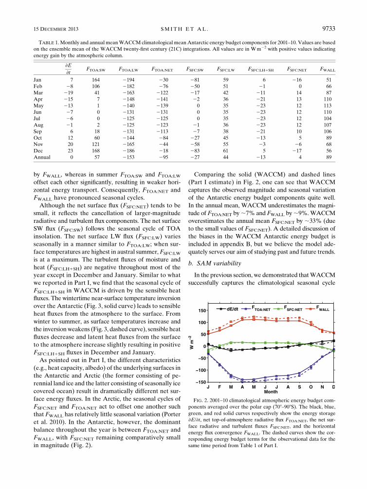
ergy storage (›E/›t) are generally small. The values for

FSFC:NET, ›E/›t, FTOA:NET, and FWALL from Table 1 are

also shown in the solid lines in Fig. 2. The climatology

shown in Fig. 2 agrees well with the observational esti-

mates of Part I (dashed lines in Fig. 2).

The net TOA radiative flux (FTOA:NET) is negative

throughout the year, indicating a net flux of energy from

the atmospheric column to space. In winter, the net TOA

SW flux, FTOA:SW, is essentially zero over the Antarctic

polar cap and the net TOALWflux,FTOA:LW, is balanced


by FWALL, whereas in summer FTOA:SW and FTOA:LW

offset each other significantly, resulting in weaker hori-

zontal energy transport. Consequently, FTOA:NET and

FWALL have pronounced seasonal cycles.

Although the net surface flux (FSFC:NET) tends to be

small, it reflects the cancellation of larger-magnitude

radiative and turbulent flux components. The net surface

SW flux (FSFC:SW) follows the seasonal cycle of TOA

insolation. The net surface LW flux (FSFC:LW) varies

seasonally in a manner similar to FTOA:LW; when sur-

face temperatures are highest in austral summer, FSFC:LW

is at a maximum. The turbulent fluxes of moisture and

heat (FSFC:LH1SH) are negative throughout most of the

year except in December and January. Similar to what

we reported in Part I, we find that the seasonal cycle of

FSFC:LH1SH in WACCM is driven by the sensible heat

fluxes. The wintertime near-surface temperature inversion

over the Antarctic (Fig. 3, solid curve) leads to sensible

heat fluxes from the atmosphere to the surface. From

winter to summer, as surface temperatures increase and

the inversionweakens (Fig. 3, dashed curve), sensible heat

fluxes decrease and latent heat fluxes from the surface

to the atmosphere increase slightly resulting in positive

FSFC:LH1SH fluxes in December and January.

As pointed out in Part I, the different characteristics

(e.g., heat capacity, albedo) of the underlying surfaces in

the Antarctic and Arctic (the former consisting of pe-

rennial land ice and the latter consisting of seasonally ice

covered ocean) result in dramatically different net sur-

face energy fluxes. In the Arctic, the seasonal cycles of

FSFC:NET and FTOA:NET act to offset one another such

that FWALL has relatively little seasonal variation (Porter

et al. 2010). In the Antarctic, however, the dominant

balance throughout the year is between FTOA:NET and

FWALL, with FSFC:NET remaining comparatively small

in magnitude (Fig. 2).

Comparing the solid (WACCM) and dashed lines

(Part I estimate) in Fig. 2, one can see that WACCM

captures the observed magnitude and seasonal variation

of the Antarctic energy budget components quite well.

In the annual mean, WACCM underestimates the magni-

tude of FTOA:NET by;7% and FWALL by;9%.WACCM

overestimates the annual mean FSFC:NET by ;33% (due

to the small values of FSFC:NET). A detailed discussion of

the biases in the WACCM Antarctic energy budget is

included in appendix B, but we believe the model ade-

quately serves our aim of studying past and future trends.

b. SAM variability

In the previous section, we demonstrated thatWACCM

successfully captures the climatological seasonal cycle

TABLE 1.Monthly and annual meanWACCMclimatological meanAntarctic energy budget components for 2001–10. Values are based

on the ensemble mean of the WACCM twenty-first century (21C) integrations. All values are in Wm22 with positive values indicating

energy gain by the atmospheric column.

›E

›tFTOA:SW FTOA:LW FTOA:NET FSFC:SW FSFC:LW FSFC:LH1SH FSFC:NET FWALL

Jan 7 164 2194 230 281 59 6 216 51

Feb 28 106 2182 276 250 51 21 0 66

Mar 219 41 2163 2122 217 42 211 14 87

Apr 215 7 2148 2141 22 36 221 13 110

May 213 1 2140 2139 0 35 223 12 113

Jun 27 0 2131 2131 0 35 223 12 110

Jul 26 0 2125 2125 0 35 223 12 104

Aug 21 2 2125 2123 21 36 223 12 107

Sep 6 18 2131 2113 27 38 221 10 106

Oct 12 60 2144 284 227 45 213 5 89

Nov 20 121 2165 244 258 55 23 26 68

Dec 23 168 2186 218 283 61 5 217 56

Annual 0 57 2153 295 227 44 213 4 89

FIG. 2. 2001–10 climatological atmospheric energy budget com-

ponents averaged over the polar cap (708–908S). The black, blue,

green, and red solid curves respectively show the energy storage

›E/›t, net top-of-atmosphere radiative flux FTOA:NET, the net sur-

face radiative and turbulent fluxes FSFC:NET, and the horizontal

energy flux convergence FWALL. The dashed curves show the cor-

responding energy budget terms for the observational data for the

same time period from Table 1 of Part I.


of the Antarctic energy budget, and is in good agree-

ment with observations. We here turn to the interannual

variability. Part I showed that the intraseasonal-to-

interannual variability of the components of the energy

budget is well correlated with large-scale modes of at-

mospheric variability, particularly the SAM. In this sec-

tion, we continue our validation of the simulation of the

Antarctic energy budget in WACCM by examining how

well it simulates the interannual correlations with the

SAM. Since the trend in the large-scale atmospheric

circulation in the Southern Hemisphere during the

twentieth-century period inWACCM is characterized by

a positive trend in the SAM (Figs. 1b,c), it is important to

validate the interannual relationships between energy

budget components and the SAM inWACCMbefore we

examine the trends.

First, we show that the horizontal energy flux con-

vergence (FWALL) and the net TOA radiative flux

(FTOA:NET) not only balance each other in the clima-

tological mean, but their detrended anomalies also

balance. Figure 4 shows a scatterplot of the annual mean

FTOA:NET and FWALL anomalies. In the annual mean,

approximately 52%of the variance inFWALL is explained

by FTOA:NET. Thus, interannual changes in one compo-

nent are coupled to changes in the other.

Second, we find that the observed annual mean cor-

relations between the SAM and the energy budget

components are well represented in WACCM. Figure 5

shows scatterplots of the annualmeanFTOA:NET (Fig. 5a),

FWALL (Fig. 5b), and FSFC:NET (Fig. 5c) anomalies and

the SAM. Note that the scale on the y axis in Fig. 5c is

different from Figs. 5a and 5b. In the annual mean, the

SAM is positively correlated with FTOA:NET (primarily

the LW flux; R2 5 0.48), negatively correlated with

FWALL (R25 0.36), and positively correlated with FSFC:NET(R2 5 0.22). These regressions are all significant at the

95% level and qualitatively agree with the observational

equivalents discussed in Part I.

Third, we compare the seasonal correlations between

the energy budget components and the SAMwith Part I

(see Table 2 herein). WACCM captures the sign and

approximate magnitude of the correlations between

FTOA:SW, FTOA:LW, and FTOA:NET and the SAM in both

June–August (JJA) and December–February (DJF)

(cf. Table 2 of Part I). We note that the negative FTOA:SW–

SAM correlation in DJF in WACCM arises primarily

from the clear-sky component of FTOA:SW, and this is due

in part to the negative correlation between total column

ozone and the SAM during this season.

Broadly, the positive annual mean correlations be-

tween FTOA:NET and the SAM reflect a decrease in out-

going LW radiation during the positive phase of the SAM

FIG. 3. Vertical profile of polar cap averaged (708–908S) tem-

perature for June–August (JJA; solid curve) and DJF (dashed

curve). Data points below the Antarctic surface are not included.

FIG. 4. Scatterplot of WACCM annual mean, piecewise, linearly

detrended polar cap averaged (708–908S) FTOA:NET and FWALL

anomalies for 1960–2065 (20C and 21C). Solid black line indicates

the least squares linear fit to the data.


when the Antarctic continent is anomalously cold. In

DJF, the positive correlation between FTOA:LW and the

SAM is offset by a negative correlation with FTOA:SW

(i.e., a decrease in absorbed solar radiation when the SAM

is positive), which results in a weaker FTOA:NET–SAM

correlation in DJF.

We also note several differences between the seasonal

correlations in WACCM and in the observations (see

Table 2 of Part I). Several of the differences are in the

surface flux correlations that are the least constrained flux

estimates in the observational energy budget of Part I

(Berrisford et al. 2011). In the remainder of this section,

we discuss the details of these differences.

In both DJF and JJA, we find positive correlations

with FSFC:SH1LH (primarily FSFC:SH) and the SAM.

Part I also showed positive correlations in both seasons

although the JJA correlation is not significant in the

observations.

The SAM correlation with FSFC:LW in JJA is also

positive in WACCM but is insignificant in the observa-

tions. The sign of this correlation requires some clarifi-

cation. There is a significant negative correlation between

the upward FSFC:LW and the SAM in JJA in WACCM,

which agrees with the negative correlation between sur-

face temperature and the SAM (not shown). However,

there is also a negative correlation between the down-

ward FSFC:LW in JJA. The net effect is that the cooling of

the atmospheric column during the positive phase of the

SAM leads to a decrease in downward FSFC:LW that ex-

ceeds the decrease in upward FSFC:LW. The cooling of the

atmospheric column also explains the positive correlation

in WACCM between FSFC:SH1LH and the SAM in JJA

due to a decrease in downward SH flux (Table 2). In the

annual mean (Fig. 5c), the main contribution to the net

surface flux is the net surface LW flux, FSFC:LW, and the

explanation for the sign of the correlation is the same as

the JJA correlation.

Finally, we find a negative correlation between FWALL

and the SAM in DJF and JJA in WACCM, again not

present in the observations. This correlation implies that

when the SAM is in its positive phase (i.e., the westerly

jet is poleward shifted), the horizontal energy flux into

Antarctica decreases. With respect to the two-way bal-

ance between FWALL and FTOA:NET, these negative

correlations in DJF and JJA agree with the positive

FTOA:NET–SAM correlations in these seasons. They

also agree with the sign of the annual mean correlation

shown in Fig. 5b.

Overall, the annual mean relationships between the

energy budget components and the SAM are well rep-

resented in WACCM, and Fig. 5 suggests that the rela-

tionships between the energy budget terms and the SAM

in the annual mean are most representative of the re-

lationships for JJA (Table 2). There are several seasonal

FIG. 5. Scatterplots of the WACCM annual mean, piecewise, linearly detrended SAM and the polar cap averaged (708–908S) (a) FTOA:NET,

(b)FWALL, and (c)FSFC:NET anomalies for 1960–2065 (20Cand 21C). Solid black lines indicate the least squares linear fit to thedata.Note that the

y axis in (c) differs from (a) and (b).

TABLE 2. DJF and JJA correlations between piecewise, linearly detrended Antarctic energy budget components and the SAM for 1960–

2065 (20C and 21C). Bold font indicates correlations that are statistically significant at the 95% level.

›E

›tFTOA:SW FTOA:LW FTOA:NET FSFC:SW FSFC:LW FSFC:LH1SH FSFC:NET FWALL

DJF 20.006 20.34 0.55 0.20 0.14 0.11 0.24 0.56 20.26

JJA 20.10 0.12 0.59 0.59 20.15 0.39 0.28 0.46 20.49


differences in the SAM correlations between WACCM

and the observations, and we note that these differences

may be due in part to the short time series of the obser-

vational record (Table 2 of Part I used data for the 2001–

10 time period only).

Having confirmed that our WACCM simulations generally

capture both the mean and the variability of the Antarctic en-

ergy budget, in the next subsection we examine the recent past

and projected future trends in theAntarctic energy budget.We

will show that accounting for the direct effect of stratospheric

ozone depletion and recovery on the radiative fluxes is crucial

for interpreting the energy budget trends.

c. Multidecadal trends: Ozone depletion and recovery

Asone can see from theblack curves inFigs. 1b and1c, the

summertime and annual meanWACCM trends in the SAM

during the twentieth-century period are positive. The largest

positive trends occur in austral summer and are associated

with springtime stratospheric ozone depletion, but weaker

positive trends are also evident in winter and spring (not

shown). Based on the above correlations between the SAM

and the net TOA radiative flux (FTOA:NET) and the re-

lationship between FTOA:NET and the horizontal energy flux

convergence, FWALL, one might expect to find a contempo-

raneous positive trend in the annual mean FTOA:NET and

negative trend in FWALL over this time period. Likewise, as

the trend in the SAM is projected to change considerably in

the future (21C), the trends in the energybudget components

may be expected to change accordingly. However, this is not

whatwefind in theWACCMsimulations. Thedepletion and

recovery of stratospheric ozone over the South Pole has

a dramatic effect on FTOA:SW, and it completely over-

whelms any effect that the SAM trends might have on

trends in the energy budget components based on the

relationships discussed in section 3b.

Figure 6a shows the time series of October–December

averaged net TOA SW flux (FTOA:SW) in WACCM.

OND is the season when stratospheric ozone depletion

occurs over the South Pole. Note that FTOA:SW de-

creases dramatically over the twentieth-century time

period when ozone depletion occurs (cf. Fig. 1a). The

decrease in net FTOA:SW is due to the fact that less

downward SW radiation is absorbed in the atmospheric

column by stratospheric ozone and therefore more SW

radiation reaches the clouds and the surface and is re-

flected back to space. Additionally, less of the reflected

upward SW is absorbed in the stratosphere by the ozone

layer. The result is an increase in upward SW and, thus,

a decrease in net SW at the TOA (FTOA:SW). The largest

contribution to the twentieth-century trend shown in

Fig. 6a results from the clear-sky component of FTOA:SW

(not shown); however, the trend is slightly amplified (an

;1Wm22 decrease from1960 to 2000) due to an increase

in total cloud fraction during this time period, shown in

Fig. 6c. The increase in total cloud fraction is associated

with the poleward shift of the storm tracks. Note that the

TOASWtrends are not associatedwith the positive trend

FIG. 6. WACCM time series of polar cap averaged OND (a)

FTOA:SW, (b) FTOA:LW, and (c) total cloud fraction. Black curve

indicates the 20C and 21C scenarios and red curve indicates the

FixODS scenario. Least squares linear fits to 20C, 21C, and Fix-

ODS are shown. Individual ensemble members are shown in thin

gray and pink curves.


in the SAM in OND as the detrended FTOA:SW–SAM

relationship in OND is not statistically significant (not

shown). Overall, the interannual relationships between

the energy budget components and the SAM inONDare

very similar to those in JJA (see Table 2).

In the twenty-first century, FTOA:SW increases as ozone

recovers in the 21C scenario, but remains relatively

constant for the FixODS scenario (Fig. 6a). Total cloud

fraction decreases slightly in the 21C scenario, comple-

menting the effect of ozone recovery on FTOA:SW, but

changes little with FixODS (Fig. 6c). The only difference

between our two twenty-first-century simulations is the

prescribed surface concentrations of ODSs, and thus

the difference in the twenty-first-century energy budget

trends can be directly and unambiguously attributed to

the differences in stratospheric ozone.

Figure 6b shows the time series of net TOA LW flux

(FTOA:LW) in OND in WACCM. Here FTOA:LW is also

altered by the changes in stratospheric ozone. During the

twentieth-century period, when ozone depletion occurs,

FTOA:LW increases due to cooling of the stratosphere and

the surface/troposphere (in accordance with the positive

trend in the SAM). Greenhouse gas forcing also con-

tributes to the cooling of the stratosphere. The increase

in FTOA:LW is about half the magnitude of the decrease in

FTOA:SW over the 1960–2000 time period, resulting in

a pronounced negative FTOA:NET trend inOND (Fig. 7a).

As ozone recovers (21C), FTOA:LW decreases, illus-

trating the combined warming of the stratosphere (due

to ozone recovery) and the surface/troposphere (due

to increases in GHG). For the FixODS scenario, the

surface/tropospherewarms but the stratosphere continues

to cool, causing a weaker decrease in FTOA:LW.

The key role of ozone depletion and recovery is

brought to light by considering the seasonal cycle of the

trends in the twentieth- and twenty-first-century periods.

Figure 7a shows themonthly twentieth-century trends for

FTOA:NET in WACCM. Negative trends are statistically

significant in austral spring, as one might expect. During

the twentieth-century period, FTOA:NET decreases because

of the decrease in FTOA:SW. Note that the detrended, in-

terannual FTOA:NET–SAM correlation inOND is positive

and statistically significant (not shown), suggesting that

a positive trend in the SAM in OND cannot explain the

negative trends in FTOA:NET in Fig. 7a.

In the twenty-first century, for the 21C scenario, the

increase in FTOA:SW results in a positive trend inFTOA:NET

in austral spring, whereas for the FixODS scenario the

decrease in FTOA:LW leads to a weak negative trend in

FTOA:NET in spring. This is shown in the differences

(21C 2 FixODS) between the FTOA:NET trends in the

twenty-first century (Fig. 7c). The differences are positive

FIG. 7. Bar plots of monthly twentieth-century (20C) trends for polar cap averaged (708–908S) (a) FTOA:NET and

(b) FWALL in Wm22 decade21. (c),(d) As in (a),(b), but showing the difference in twenty-first century trends

(21C 2 FixODS). Statistical significance is shown by the crosses (95%) and double crosses (99%).


and statistically significant at the 95% level in OND. The

statistically significant FTOA:NET trend differences in

April and May reflect two processes; first, ozone re-

covery from an approximate 15% loss occurs in these

months, which leads to increased absorbed SW radiation,

and second, significant sea ice loss near the continent

in the FixODS scenario relative to the 21C scenario

leads to enhanced warming near the Antarctic coast

(see Fig. 3b of Smith et al. 2012) and increased outgoing

LW radiation. Studies have shown that the climate ef-

fects of independently prescribed GHG forcing and

ozone recovery in GCMs are approximately additive

(Polvani et al. 2011a; McLandress et al. 2011); thus, the

effect of GHG forcing on FTOA:NET roughly subtracts

out in Fig. 7c.

For both the twentieth- and twenty-first-century periods,

the trends in OND FTOA:NET are evident in like-signed

trends in the energy tendency, ›E/›t, for the same season

(not shown).Notably, these trends inFTOA:NET coincidewith

opposite-signed trends in the SAM, particularly in Decem-

ber. In other words, the positive interannual correlation be-

tween the SAM and FTOA:NET described in section 3b is

nowhere to be seen in the trends. Again, this shows that

stratospheric ozone is the controlling factor, and the

SAM does not give useful information about long-term

trends (contrast Figs. 1b and 7a,c).

Having examined FTOA:NET, we now turn to the

horizontal energy flux convergence, FWALL. Figure 7b

shows the monthly twentieth-century trends for FWALL

in WACCM. Austral summer is the season that experi-

ences the largest positive trends in FWALL, particularly

in January when the trend is statistically significant at the

95% level. Note that while the trend in FWALL is positive,

there is also a positive trend in the SAM in summer

during the twentieth-century period (Fig. 1b) that runs

counter to the interannual relationship between the

summer SAM and FWALL shown in Table 2. Although an

investigation of the dynamical mechanisms that drive the

trends in FWALL is beyond the scope of this paper, it is

clear that the trends in FWALL act to compensate for the

trends in FTOA:NET one to two months earlier.

In the twenty-first century, the trend in FWALL re-

verses sign in summer as ozone recovers and is weakly

positive for the FixODS scenario (not shown). The dif-

ferences between the FWALL trends in the two twenty-

first-century scenarios (21C 2 FixODS) are shown in

Fig. 7d and are statistically significant at the 95% level in

January. For both the twentieth- and twenty-first-century

scenarios, the FWALL trends are reflected in like-signed

trends in ›E/›t during the summer season (not shown).

As for the net surface flux (FSFC:NET), there are no

significant trends in the 20C, 21C, or FixODS simulations

in anymonth (not shown). This further demonstrates that

the two-way balance between FTOA:NET and FWALL in

the Antarctic region found in the climatological mean

and on intraseasonal-to-interannual time scales also car-

ries over to the multidecadal time scale changes consid-

ered here. This balance, characteristic of the Antarctic

and very much unlike the Arctic, appears to hold on all

time scales.

Finally, the annual mean trends in the Antarctic at-

mospheric energy budget are shown in Fig. 8. The annual

mean time series of FTOA:NET (Fig. 8a) shows a negative

trend during the decades of ozone depletion. In the

twenty-first century as ozone recovers (21C), there is very

little trend in FTOA:NET due to opposite-signed trends in

FTOA:LW and FTOA:SW, with the SW changes being con-

fined to the OND season and the LW changes occurring

throughout the year. The effect of future GHG forcing

alone on the annual mean FTOA:NET is clearly seen in the

FixODS scenario, indicating a weak but significant neg-

ative trend due to increased outgoing LW radiation.

Figure 8b shows the annualmean time series of FWALL.

During the twentieth-century period, the negative trend

in FTOA:NET (Fig. 8a) is balanced by a positive trend in

FWALL. For the 21C scenario, Fig. 8b depicts a relatively

flat trend, consistent with the weak trend in FTOA:NET for

the same scenario. For the FixODS scenario, which rep-

resents the effect ofGHG forcing alone, a positiveFWALL

trend balances the negative trend in FTOA:NET. Thus,

Fig. 8 suggests that projected ozone recovery mitigates

the increase in horizontal energy flux into the Antarctic

polar cap associated with GHG warming.

4. Summary and conclusions

In this paper, we have extended our examination of the

Antarctic atmospheric energy budget using an ensemble of

integrations of the CESM1(WACCM) climate model.

We find that WACCM reproduces the climatological

energy budget reasonably well relative to the obser-

vational estimate presented in Part I. In addition, we

have shown that WACCM is able to capture the ob-

served interannual relationships between the energy

budget terms and the SAM. A large fraction of the

interannual variability in the energy budget terms can

be explained by the SAM, particularly in austral winter.

In the annual mean, the net TOA radiative flux, FTOA:

NET, and the horizontal energy flux convergence, FWALL,

are positively and negatively correlated with the SAM,

respectively.

From an energy balance perspective, the opposite-

signed interannual correlations reflect the fact that,

seasonally and in the annual mean, energy balance

over theAntarctic polar cap is primarily satisfied through

compensating changes in FWALL and FTOA:NET. From a


dynamical perspective, however, the negative correlation

between FWALL and the SAM might seem counterintui-

tive. During the positive phase of the SAM the baroclinic

zone is shifted poleward and one would naively guess

this would result in larger energy flux into the polar cap

by synoptic eddies; yet the opposite is found in both

WACCM and the reanalysis (Part I). Weaker energy

flux during the positive phase of the SAM suggests that

synoptic eddies may become less efficient at trans-

porting energywith a poleward-displaced baroclinic zone

(Carleton and Whalley 1988). This dynamical interpre-

tation is complicated, however, by the fact that the

twentieth-century summertime trend in FWALL is positive

when the SAM is trending positive and the westerly jet is

shifting poleward. Our investigation of the nature of the

relationship between FWALL and the SAM is ongoing.

On multidecadal time scales, the effects of ozone de-

pletion and projected recovery dominate the trends in

the Antarctic energy budget from 1960 to 2065. During the

twentieth-century period from 1960 to 2000, ozone depletion

results in an annual mean decrease in FTOA:NET due to the

decrease inFTOA:SW.This isbalancedbyan increase inFWALL.

In the twenty-first century as ozone recovers, the opposite-

signed trends in the net TOA SW and LW fluxes (FTOA:

SW and FTOA:LW) result in little trend in FTOA:NET and

consequently FWALL. An alternative twenty-first-century

scenario in which GHGwarming occurs in the absence of

ozone recovery shows a continued increase in FWALL in

the future. Thus, the future positive trend in energy flux

convergence into the Antarctic polar cap due to GHG

warming is mitigated by ozone recovery.

This study highlights the fact that the annual mean

interannual correlations between the SAMand FTOA:NET

andFWALL do not help to explain themultidecadal trends

in these fluxes. Smith et al. (2012) arrived at a similar

conclusion with respect to the SAM andAntarctic sea ice

trends. Although the SAM is a good predictor of in-

terannual variations in Antarctic climate, we emphasize

that the SAM may not be a good predictor of multi-

decadal trends in the Antarctic climate system and we

caution against using the SAM as a means of explaining

trends.

The role of energy flux convergence in futureAntarctic

polar amplification is currently unknown. As GCMs do

not yet include dynamic Antarctic ice sheet and ice shelf

components, it is unclear how increases in well-mixed

GHGs and ozone recovery will affect the Antarctic sur-

face energy balance in the future and how changes in

the surface energy balance will be compensated for by

changes in other components of the Antarctic atmo-

spheric energy budget. OurWACCM simulations show

no statistically significant trend in FSFC:NET in either the

21C or FixODS twenty-first-century scenarios. Despite

current model limitations, our work suggests that the ef-

fect of ozone recovery in the future may mask the effect

of GHG warming on the Antarctic energy budget for

several decades.

Acknowledgments. The authors would like to grate-

fully acknowledge the NSFAntarctic Sciences Program,

ANT-09-44063. The CESM Project is supported by the

National Science Foundation (NSF) and the Office of

Science (BER) of the U.S. Department of Energy. All

model integrations were performed at the National Cen-

ter for Atmospheric Research (NCAR), which is spon-

sored by the U.S. NSF.We thankDanMarsh, MikeMills,

andDougKinnison at NCAR for their assistance with the

model integrations.

FIG. 8. As in Fig. 6, but for annual mean (a) FTOA:NET and (b) FWALL.


APPENDIX A

Vertically Integrated Atmospheric Energy BudgetDerivation

Some of the steps needed to obtain Eqs. (1)–(5) are

mentioned in the literature (e.g., Trenberth and Solomon

1994; Trenberth 1997). However, we were unable to find

a complete and coherent derivation of these equations

from first principles. Hence, for the sake of completeness,

we include it here with enough detail to make the deri-

vation easily understandable. We start with the thermo-

dynamic equation,

cp

�›T

›t1 v � $T1v

�›T

›p2 k

T

p

��5Q , (A1)

where T is temperature, v is the horizontal wind vector,

v is the vertical wind component, p is pressure, cp is the

isobaric specific heat capacity, k is the ratio of the

specific gas constant, R, to cp, and Q is the diabatic

heating. The kinetic energy equation is obtained by tak-

ing the dot product of the horizontal momentum equa-

tions with v,

›k

›t1$ � kv1 ›kv

›p52v � $F1 v � F , (A2)

where k is the kinetic energy, F is the geopotential, and

F is friction. Neglecting frictional dissipation and using

the ideal gas law, the hydrostatic equation and the con-

tinuity equation, the sum of Eqs. (A1) and (A2) can be

written as

›(cpT1 k)

›t1$ � (cpT1F1 k)v

1›(cpT1F1 k)v

›p5Q . (A3)

Next, we add the moisture equation to Eq. (A3) to

obtain

›(cpT1 k1Lq)

›t1$ � (cpT1F1 k1Lq)v

1›(cpT1F1 k1Lq)v

›p5Q1L(e2 c) , (A4)

where q is the specific humidity, L is the latent heat of

vaporization for water, e is the rate of evaporation, and

c is the rate of condensation within the atmosphere per

unit mass. Now, we vertically integrate Eq. (A4) and

use the Leibniz rule to take ›/›t and $� outside of the

integrals. The terms on the left-hand side of Eq. (A4)

become

ðps

0

›(cpT1 k1Lq)

›t

dp

g5

›

›t

ðps

0(cpT1 k1Lq)

dp

g

21

g(cpT1 k1Lq)jp

s

›ps›t

,

(A5)

ðps

0$ � (cpT1F1 k1Lq)v

dp

g

5$ �ðp

s

0(cpT1F1 k1Lq)v

dp

g

21

g(cpT þFþ k1Lq)vjp

s� $ps , (A6)

and

ðps

0

›(cpT1F1 k1Lq)

›p

dp

g5

1

g(cpT1F1 k1Lq)vjp

s,

(A7)

where subscript s indicates the surface value. To reduce

these terms to the form outlined in section 2b, we use the

definition of v evaluated at the surface,

vs 5›ps›t

1 vs � $ps . (A8)

Substituting vs in Eq. (A7) for Eq. (A8), and sub-

stituting Eqs. (A5)–(A7) in the vertically integrated Eq.

(A4), many of the terms cancel and we end up with

›

›t

ðps

0(cpT1 k1Lq)

dp

g

1$ �ðp

s

0(cpT1F1 k1Lq)v

dp

g

21

gFsvs � $ps 1

1

gFsvs 5

ðps

0[Q1L(e2 c)]

dp

g.

(A9)

Substituting Eq. (A8) into Eq. (A9), and rearranging

the partial derivatives, we get

›

›t

ðps

0(cpT1 k1Lq)

dp

g

1$ �ðp

s

0(cpT1F1 k1Lq)v

dp

g1

1

g

›psFs

›t

5

ðps

0[Q1L(e2 c)]

dp

g. (A10)

Finally, taking the ›psFs/›t inside the integral gives


›

›t

ðps

0(cpT1k1Lq1Fs)

dp

g

1$ �ðp

s

0(cpT1F1k1Lq)v

dp

g

5

ðps

0[Q1L(e2 c)]

dp

g. (A11)

The left-hand side of Eq. (A11) is now in the form

shown in section 2b. The right-hand side of Eq. (A11)

can be rewritten as

ðps

0[Q1L(e2 c)]

dp

g5FTOA:NET 1FSFC:RAD 1FSFC:SH

1LP1L(E2P) ,

(A12)

where FTOA:NET is the net radiative flux at the top of the

atmosphere, FSFC:RAD is the net radiative flux at the

surface, FSFC:SH is the surface sensible heat flux, and P

and E are the precipitation and the surface evaporation

rates; LE is equivalent to the surface latent heat flux,

FSFC:LH. Thus, the complete energy budget equation as

outlined in section 2b is as follows:

›

›t

ðps

0(cpT1k1Lq1Fs)

dp

g

1$ �ðp

s

0(cpT1F1k1Lq)v

dp

g

5FTOA:NET1FSFC:NET , (A13)

where FTOA:NET and FSFC:NET are as defined in Eqs. (3)

and (4) in section 2b.

APPENDIX B

Antarctic Atmospheric Energy Budget Biases inWACCM

a. Data

We use several observational data products to ex-

amine the biases in the Antarctic atmospheric energy

budget in WACCM. We use the CERES satellite data

of TOA radiative fluxes from 2001 to 2010. Monthly

CERES TOA fluxes from the Energy Balanced and

Filled (EBAF) dataset are obtained on a 18 3 18 gridfrom the National Aeronautics and Space Administra-

tion (NASA) Langley Research Center Atmospheric

Science Data Center. To produce the EBAF data,

CERESTOA shortwave (SW) and longwave (LW) fluxes

are adjusted such that the global mean net TOA flux

(averaged over several years) is equal to the estimated

present-day change in heat storage in the Earth system

(Loeb et al. 2009). This procedure thus eliminates the

unrealistically large global mean TOA flux that exists

in the unadjusted CERES data (Trenberth et al. 2009).

We also use the associated computed CERES surface

radiative flux product for 2001–10 (Kratz et al. 2010).

To assess the model-simulated cloud cover, we use

satellite-derived total cloud fraction and cloud mean

water path from the International Satellite Cloud Cli-

matology Project (ISCCP), which provides complete

spatial coverage of the Antarctic polar cap (Rossow and

Schiffer 1999). Climatological monthly mean ISCCP

fields based on data from July 1983 toDecember 2009 are

obtained on a 2.58 3 2.58 grid from the NASA Goddard

Institute for Space Studies.

Column ozone inWACCM is compared to theAC&C/

SPARC (expansion below) ozone database for 2001–09.

This database was created as a joint effort between the

Chemistry–Climate Modeling Validation (CCMVal) Ac-

tivity of the World Meteorological Organization’s Strato-

spheric Processes and their Role in Climate (SPARC)

project and the Atmospheric Chemistry and Climate

(AC&C) Initiative, for use as a forcing for CMIP5 gen-

eral circulation models (GCMs) that do not include

interactive ozone chemistry (Cionni et al. 2011). For

2001–09, the AC&C/SPARC stratospheric ozone da-

tabase is generated in a manner similar to Randel and

Wu (2007).

Lastly, we compareWACCM surface air temperature

(SAT) for 2001–10 to observations from 18 Antarctic

weather stations (see Fig. 1 in Part I). These observations

were made available as part of the Reference Antarctic

Data for Environmental Research (READER) project

(Turner and Colwell 2004).

b. Model biases

Figure B1a shows the TOA biases in WACCM rela-

tive to CERES for the 2001–10 period. The blue curve

shows the FTOA:NET bias relative to CERES, which is

positive throughout the year except in December. The

positive bias in FTOA:NET arises primarily from the posi-

tive bias in the FTOA:LW component, while the negative

FTOA:NET bias in December arises from the negative bias

in FTOA:SW (solid red curve).

In general, there is no consensus on the sign of FTOA:

LW biases in the Antarctic across reanalyses and GCMs

(Trenberth and Fasullo 2010). The positive bias in

WACCM ismainly due to the cold SAT bias inWACCM

over the Antarctic region. Figure B1b (black curve)

shows the WACCM SAT relative to Antarctic station

data from READER (see Fig. 1 of Part I for station

locations). The seasonal cycle of the WACCM FTOA:LW

bias (Fig. 9a) generally agrees with the SAT bias.


In addition to the surface air temperature bias,

WACCM displays a negative stratospheric ozone bias

(Fig. B1d; polar cap averaged (708–908S) and column

integrated between 500 and 1hPa) relative to theAC&C/

SPARC ozone database for the time period 2001–09.

The ozone bias may also be contributing to the positive

FTOA:LW bias in WACCM, particularly in austral spring.

A negative bias in ozone cools the stratosphere due to

a decrease in absorption of SW radiation. Indeed, the

lower stratosphere in WACCM is known to be biased

cold (Marsh et al. 2013). The AC&C/SPARC ozone

database is constructed using satellite and ozonesonde

data and may itself be biased somewhat high in the

Antarctic relative to other observationally based ozone

climatologies (Hassler et al. 2012).

The SW biases in WACCM (Fig. B1a) are not typical

of reanalyses and GCMs (Trenberth and Fasullo 2010).

Trenberth and Fasullo (2010) show that reanalyses and

GCMs typically overestimate FTOA:SW at high southern

latitudes. In contrast,WACCMunderestimates FTOA:SW,

particularly in austral spring and summer. The Com-

munity Climate System Model version 3 (CCSM3) was

also shown to underestimate FTOA:SW over the Antarctic

polar cap (Briegleb and Bromwich 1998). In fall, a nega-

tive WACCM bias in upward FTOA:SW is partially offset

by a positive bias in downward solar flux in WACCM

relative toCERES (dotted red curve, Fig. B1a). In spring,

a fraction of the negative WACCM bias in FTOA:SW can

be attributed to too little downward solar flux at the top of

the atmosphere. The remainder of the negative bias is

explained by the fact thatWACCM is reflectingmore SW

radiation from the surface and atmosphere back to space

compared to CERES (dashed red curve, Fig. B1a). We

attribute this to WACCM’s positive bias in surface al-

bedo (Fig. B1b) and negative bias in stratospheric ozone

(Fig. B1d).

Figure B1b shows WACCM’s polar cap averaged

surface albedo bias relative to CERES (red curve). Dur-

ing polar night, we are unable to get a reliable estimate

of the surface albedo from CERES SW fluxes. The

WACCM bias in surface albedo results in a positive bias

in upwardFSFC:SW in themodel (Fig. B1b, blue curve). To

verify that the FTOA:SW bias is not directly related to

biases in the simulated cloud fields, we plot theWACCM

biases in total cloud amount (CLDTOT) and cloud mean

water path (CLDMWP) relative to ISCCP in Fig. B1c. It

FIG. B1. (a) 2001–10 WACCM biases in top-of-atmosphere radiative fluxes (i.e., WACCM minus CERES). The

solid blue, black, and red curves show the FTOA:NET bias, FTOA:LW bias, and FTOA:SW bias relative to CERES. The

dotted and dashed red curves show the downward and upward components of the FTOA:SW bias relative to CERES.

(b) 2001–10WACCM biases in surface air temperature (SAT) relative to Antarctic station data (black curve), polar

cap averaged (708–908S) surface albedo relative to CERES (red curve), and polar cap averaged (708–908S) upwardFSFC:SW relative to CERES (blue curve). To calculate the SAT bias, the nearest WACCM grid point to each

READER station was selected and the SAT bias was averaged over all selected grid points. (c) 1983–2009WACCM

biases in total cloud fraction, CLDTOT (black curve), and total cloud mean water path, CLDMWP (red curve),

relative to ISCCP. (d) 2001–09WACCMbias in column ozone (polar cap averaged and vertically integrated from 500

to 1 hPa) relative to the AC&C/SPARC ozone database.


is important to note that there are challenges when

comparing model-simulated cloud data with satellite-

derived data, particularly in polar regions where satellite

products contain significant biases (Bromwich et al. 2012).

For example, ISCCP, which is based on passive visible–

infrared (VIS-IR) retrievals, is missing CLDMWP in-

formation at high latitudes from February through

September due to very low insolation during thesemonths.

Unlike theCMIP3models andCCSM3, which typically

overestimate cloud amount over the Antarctic polar cap

throughout the year (Bromwich et al. 2012; Briegleb and

Bromwich 1998), WACCM tends to underestimate cloud

amount in late spring, summer, and fall and overestimate

in winter and early spring. When the FTOA:SW bias is

largest in late austral spring, WACCM has negative bia-

ses in both CLDTOT and CLDMWP (Fig. B1c). This

indicates that the negative bias in FTOA:SW is likely not

due to increased SW reflection back to space due to a

greater amount of brighter clouds in WACCM. In fact,

the negative biases in cloud properties in WACCM act

to amplify the effect of the surface albedo bias on the

FTOA:SW bias. A detailed analysis of the cloud properties

in WACCM is beyond the scope of this study.

The negative bias in stratospheric ozone may also

contribute to the negative FTOA:SW bias in WACCM.

A negative bias in ozone indicates that less SW radi-

ation is absorbed by ozone and is therefore available to

be reflected back to space by the surface, clouds, and

atmosphere.

REFERENCES

Berrisford, P., P. K�allberg, S. Kobayashi, D. Dee, S. Uppala, A. J.

Simmons, P. Poli, and H. Sato, 2011: Atmospheric conserva-

tion properties in ERA-Interim. Quart. J. Roy. Meteor. Soc.,

137, 1381–1399, doi:10.1002/qj.864.

Briegleb, B., and D. Bromwich, 1998: Polar radiation budgets of

the NCAR CCM3. J. Climate, 11, 1246–1269.Bromwich, D., and Coauthors, 2012: Tropospheric clouds in Antarc-

tica. Rev. Geophys., 50, RG1004, doi:10.1029/2011RG000363.

Carleton,A., andD.Whalley, 1988: Eddy transport of sensible heat

and the life history of synoptic systems: A statistical analysis

for the Southern Hemisphere winter.Meteor. Atmos. Phys., 38,

140–152.

Cionni, I., and Coauthors, 2011: Ozone database in support of

CMIP5 simulations: Results and corresponding radiative

forcing. Atmos. Chem. Phys., 11, 11 267–11 292, doi:10.5194/

acp-11-11267-2011.

Cullather, R. I., and M. G. Bosilovich, 2012: The energy budget

of the polar atmosphere in MERRA. J. Climate, 25, 5–24.

Dee, D. P., and Coauthors, 2011: The ERA-Interim reanalysis:

Configuration and performance of the data assimilation sys-

tem. Quart. J. Roy. Meteor. Soc., 137, 553–597, doi:10.1002/

qj.828.

Fasullo, J. T., and K. E. Trenberth, 2008: The annual cycle of the

energy budget. Part II: Meridional structures and poleward

transports. J. Climate, 21, 2313–2325.

Gent, P. R., and Coauthors, 2011: The Community Climate System

Model version 4. J. Climate, 24, 4973–4991.

Genthon, C., and G. Krinner, 1998: Convergence and disposal of

energy andmoisture on theAntarctic polar cap fromECMWF

reanalyses and forecasts. J. Climate, 11, 1703–1716.

Hassler, B., P. J. Young, R. W. Portmann, G. E. Bodeker, J. S.

Daniel, K. H. Rosenlof, and S. Solomon, 2012: Comparison of

three vertically resolved ozone data bases: Climatology, trends

and radiative forcings.Atmos. Chem. Phys. Discuss., 12, 26561–

26605, doi:10.5194/acpd-12-26561-2012.

Kang, S. M., L. M. Polvani, J. C. Fyfe, and M. Sigmond, 2011:

Impact of polar ozone depletion on subtropical precipitation.

Science, 332, 951–954, doi:10.1126/science.1202131.

Kay, J. E.,M.M.Holland, C.M. Bitz, E. Blanchard-Wrigglesworth,

A. Gettelman, A. Conley, and D. Bailey, 2012: The influence

of local feedbacks and northward heat transport on the equi-

librium Arctic climate response to increased greenhouse gas

forcing. J. Climate, 25, 5433–5450.

Kistler, R., E. Kalnay, and W. Collins, 2001: The NCEP–NCAR

50-Year Reanalysis: Monthly means CD-ROM and documen-

tation. Bull. Amer. Meteor. Soc., 82, 247–267.

Kratz, D. P., S. K. Gupta, A. C. Wilber, and V. E. Sothcott, 2010:

Validation of the CERES edition 2B surface-only flux algo-

rithms. J. Appl. Meteor. Climatol., 49, 164–180.

Lee, S., and S. B. Feldstein, 2013: Detecting ozone- and greenhouse

gas–driven wind trends with observational data. Science, 339,

563–567, doi:10.1126/science.1225154.

Loeb, N. G., B. A. Wielicki, D. R. Doelling, G. L. Smith, D. F.

Keyes, S. Kato, N. Manalo-Smith, and T. Wong, 2009: Toward

optimal closure of the earth’s top-of-atmosphere radiation

budget. J. Climate, 22, 748–766.

Marsh, D. R., M. J. Mills, D. E. Kinnison, J.-F. Lamarque, N. Calvo,

and L. M. Polvani, 2013: Climate change from 1850 to 2005

simulated in CESM1(WACCM). J. Climate, 26, 7372–7391.Marshall, G., 2003: Trends in the southern annular mode from

observations and reanalyses. J. Climate, 16, 4134–4143.

McLandress, C., T. G. Shepherd, J. F. Scinocca, D. A. Plummer,

M. Sigmond, A. I. Jonsson, andM. C. Reader, 2011: Separating

the dynamical effects of climate change and ozone depletion.

Part II: Southern Hemisphere troposphere. J. Climate, 24,

1850–1868.

Meinshausen, M., and Coauthors, 2011: The RCP greenhouse gas

concentrations and their extensions from 1765 to 2300. Cli-

matic Change, 109, 213–241, doi:10.1007/s10584-011-0156-z.

Nakamura, N., andA.Oort, 1988: Atmospheric heat budgets of the

polar regions. J. Geophys. Res., 93 (D8), 9510–9524.

Polvani, L.M.,M. Previdi, andC. Deser, 2011a: Large cancellation,

due to ozone recovery, of future Southern Hemisphere at-

mospheric circulation trends.Geophys. Res. Lett., 38, L04707,

doi:10.1029/2011GL046712.

——, D. W. Waugh, G. J. P. Correa, and S.-W. Son, 2011b:

Stratospheric ozone depletion: The main driver of twentieth-

century atmospheric circulation changes in the Southern

Hemisphere. J. Climate, 24, 795–812.

Porter, D. F., J. J. Cassano, M. C. Serreze, and D. N. Kindig,

2010: New estimates of the large-scale Arctic atmospheric

energy budget. J. Geophys. Res., 115, D08108, doi:10.1029/

2009JD012653.

Previdi, M., K. L. Smith, and L. M. Polvani, 2013: The Antarctic at-

mospheric energy budget. Part I: Climatology and intraseasonal-

to-interannual variability. J. Climate, 26, 6406–6418.

Randel, W. J., and F. Wu, 2007: A stratospheric ozone profile data

set for 1979–2005: Variability, trends, and comparisons with


column ozone data. J. Geophys. Res., 112, D06313, doi:10.1029/

2006JD007339.

Rossow,W. B., and R.A. Schiffer, 1999: Advances in understanding

clouds from ISCCP. Bull. Amer. Meteor. Soc., 80, 2261–2287.Sall�ee, J. B., K. G. Speer, and S. R. Rintoul, 2010: Zonally asym-

metric response of the Southern Ocean mixed-layer depth to

the southern annularmode.Nat.Geosci., 3, 273–279, doi:10.1038/

ngeo812.

Serreze, M. C., A. P. Barrett, A. G. Slater, M. Steele, J. Zhang,

and K. E. Trenberth, 2007: The large-scale energy budget

of the Arctic. J. Geophys. Res., 112, D11122, doi:10.1029/

2006JD008230.

Smith, K. L., L. M. Polvani, andD. R.Marsh, 2012: Mitigation of 21st

century Antarctic sea ice loss by stratospheric ozone recovery.

Geophys. Res. Lett., 39, L20701, doi:10.1029/2012GL053325.

Son, S.-W., N. F. Tandon, L. M. Polvani, and D. W. Waugh, 2009:

Ozone hole and Southern Hemisphere climate change. Geo-

phys. Res. Lett., 36, L15705, doi:10.1029/2009GL038671.

——, and Coauthors, 2010: Impact of stratospheric ozone on Southern

Hemisphere circulation change: A multimodel assessment.

J. Geophys. Res., 115, D00M07, doi:10.1029/2010JD014271.

Steig, E. J., D. P. Schneider, S. D. Rutherford, M. E. Mann, J. C.

Comiso, and D. T. Shindell, 2009: Warming of the Antarctic

ice-sheet surface since the 1957 International Geophysical

Year. Nature, 457, 459–462, doi:10.1038/nature07669; Corri-

gendum, 460, 766.

Thompson, D. W. J., S. Solomon, P. J. Kushner, M. H. England,

K. M. Grise, and D. J. Karoly, 2011: Signatures of the Ant-

arctic ozone hole in Southern Hemisphere surface climate

change. Nat. Geosci., 4, 741–749, doi:10.1038/ngeo1296.Trenberth, K. E., 1991: Climate diagnostics from global analyses:

Conservation of mass in ECMWF analyses. J. Climate, 4, 707–

722.

——, 1997: The definition of El Ni~no. Bull. Amer. Meteor. Soc., 78,2771–2777.

——, and A. Solomon, 1994: The global heat balance: Heat trans-

ports in the atmosphere and ocean. Climate Dyn., 10, 107–134.

——, and J. T. Fasullo, 2010: Simulation of present-day and twenty-

first-century energy budgets of the southern oceans. J. Climate,

23, 440–454.

——, ——, and J. Kiehl, 2009: Earth’s global energy budget. Bull.

Amer. Meteor. Soc., 90, 311–323.

Turner, J., and S. Colwell, 2004: The SCAR READER project:

Toward a high-quality database of mean Antarctic meteoro-

logical observations. J. Climate, 17, 2890–2898.Waugh, D. W., F. Primeau, T. Devries, and M. Holzer, 2013: Re-

cent changes in the ventilation of the southern oceans. Science,

339, 568–570, doi:10.1126/science.1225411.

WMO, 2010: Scientific assessment of ozone depletion: 2010. Global

Ozone Research and Monitoring Project Rep. 52, 516 pp.

[Available online at http://www.esrl.noaa.gov/csd/assessments/

ozone/2010/report.html.]


http://www.esrl.noaa.gov/csd/assessments/ozone/2010/report.html

http://www.esrl.noaa.gov/csd/assessments/ozone/2010/report.html

the antarctic atmospheric energy budget. part ii:...

Documents