the andrews-gordon identities and -multinomial · the andrews-gordon identities and q-multinomial...
TRANSCRIPT

THE ANDREWS-GORDON IDENTITIES AND q-MULTINOMIAL
COEFFICIENTS
S. OLE WARNAAR
Abstract. We prove polynomial boson-fermion identities for the generating function of the number
of partitions of n of the form n =PL−1
j=1 jfj , with f1 ≤ i − 1, fL−1 ≤ i′ − 1 and fj + fj+1 ≤ k.
The bosonic side of the identities involves q-deformations of the coefficients of xa in the expansion of(1+x+ · · ·+xk)L. A combinatorial interpretation for these q-multinomial coefficients is given usingDurfee dissection partitions. The fermionic side of the polynomial identities arises as the partitionfunction of a one-dimensional lattice-gas of fermionic particles.
In the limit L → ∞, our identities reproduce the analytic form of Gordon’s generalization ofthe Rogers–Ramanujan identities, as found by Andrews. Using the q → 1/q duality, identities are
obtained for branching functions corresponding to cosets of type (A(1)1 )k × (A
(1)1 )ℓ/(A
(1)1 )k+ℓ of
fractional level ℓ.
1. Introduction
The Rogers–Ramanujan identities can be stated as the following q-series identities.
Theorem 1 (Rogers–Ramanujan). For a = 0, 1 and |q| < 1,
(1.1)∞∑
n=0
qn(n+a)
(1 − q)(1 − q2) . . . (1 − qn)=
∞∏
j=0
(1 − q5j+1+a)−1(1 − q5j+4−a)−1.
Since their independent discovery by Rogers [37–39], Ramanujan [35] and also Schur [43], manybeautiful generalizations have been found, mostly arising from partition-theoretic or Lie-algebraicconsiderations, see [6, 33] and references therein.
Most surprising, in 1981 Baxter rediscovered the Rogers–Ramanujan identities (1.1) in his calcu-lation of the order parameters of the hard-hexagon model [13], a lattice gas of hard-core particles ofinterest in statistical mechanics. It took however another ten years to fully realize the power of the(solvable) lattice model approach to finding q-series identities. In particular, based on a numericalstudy of the eigenspectrum of the critical three-state Potts model [20, 31] (yet another lattice modelin statistical mechanics), the Stony Brook group found an amazing variety of new q-series identitiesof Rogers–Ramanujan type [29, 30]. Almost none of these identities had been encountered previouslyin the context of either partition theory or the theory of infinite dimensional Lie algebras.
More specific, in the work of [29,30] expressions for Virasoro characters were given through systemsof fermionic quasi-particles. Equating these fermionic character forms with the well-known Rocha-Caridi type bosonic expressions [36], led to many q-series identities for Virasoro characters, generalizingthe Rogers–Ramanujan identities (which are associated to the M(2, 5) minimal model).
The proof of the Rogers–Ramanujan identities by means of an extension to polynomial identitieswhose degree is determined by a fixed integer L, was initiated by Schur [43]. Before we elaborate onthis approach, we need the combinatorial version of the Rogers–Ramanujan identities stating that
1

2 S. OLE WARNAAR
Theorem 2 (Rogers–Ramanujan). For a = 0, 1, the partitions of n into parts congruent to 1 + a or4−a (mod 5) are equinumerous with the partitions of n in which the difference between any two partsis at least 2 and 1 occurs at most 1 − a times.
Denoting the number of occurences of the part j in a partition by fj , the second type of partitionsin the above theorem are those partitions of n =
∑
j≥1 jfj which satisfy the following frequencyconditions :
fj + fj+1 ≤ 1 ∀j and f1 ≤ 1 − a.
Schur notes that imposing the additional condition fj = 0 for j ≥ L + 1, the generating function ofthe “frequency partitions” satisfies the recurrence
(1.2) gL = gL−1 + qLgL−2.
Together with the appropriate initial conditions, Schur was able to solve these recurrences, to obtainan alternating-sign type solution, now called a bosonic expression. Taking L → ∞ in these bosonicpolynomials yields (after use of Jacobi’s triple product identity) the right-hand side of (1.1). Sincethis indeed corresponds to the generating function of the “ (mod 5)” partitions, this proves Theo-rem 2. Much later, Andrews [3] obtained a solution to the recurrence relation as a finite q-series withmanifestly positive integer coefficients, now called a fermionic expression. Taking L → ∞ in thesefermionic polynomials yields the left-hand side of (1.1).
Recently much progress has been made in proving the boson-fermion identities of [29,30] (and gen-eralizations thereof), by following the Andrews–Schur approach. That is, for many of the Virasoro-character identities, finitizations to polynomial boson-fermion identities have been found, which couldthen be proven either fully recursively (a la Andrews) or one side combinatorially and one side recur-sively (a la Schur), see [14–17,19, 22–24,26, 32, 34, 41, 42,44–46].
In this paper we consider polynomial identities which imply the Andrews–Gordon generalizationof the Rogers–Ramanujan identities. First, Gordon’s theorem [27], which provides a combinatorialgeneralization of the Rogers–Ramanujan identities, reads
Theorem 3 (Gordon). For all k ≥ 1, 1 ≤ i ≤ k + 1, let Ak,i(n) be the number of partitions of n intoparts not congruent to 0 or ±i (mod 2k + 3) and let Bk,i(n) be the number of partitions of n of theform n =
∑
j≥1 jfj, with f1 ≤ i − 1 and fj + fj+1 ≤ k (for all j). Then Ak,i(n) = Bk,i(n).
Subsequently the following analytic counterpart of this result was obtained by Andrews [5], gener-alizing the analytic form (1.1) of the Rogers–Ramanujan identities.
Theorem 4 (Andrews). For all k ≥ 1, 1 ≤ i ≤ k + 1 and |q| < 1,
(1.3)∑
n1,n2,...,nk≥0
qN21+···+N2
k+Ni+···+Nk
(q)n1(q)n2
· · · (q)nk
=∞∏
j=1j 6≡0,±i (mod 2k+3)
(1 − qj)−1
with
(1.4) Nj = nj + · · · + nk
and (q)a =∏a
k=1(1 − qk) for a > 0 and (q)0 = 1.
Application of Jacobi’s triple product identity admits for a rewriting of the right-hand side of (1.3)to
(1.5)1
(q)∞
∞∑
j=−∞
(−)jqj(
(2k+3)(j+1)−2i)
/2.
THE ANDREWS-GORDON IDENTITIES AND q-MULTINOMIAL COEFFICIENTS 3
Equating (1.5) and the left-hand side of (1.3), gives an example of a boson-fermion identity. Herewe consider, in the spirit of Schur, a “natural” finitization of Gordon’s frequency condition such thatthis boson-fermion identity is a limiting case of polynomial identities. In particular, we are interestedin the quantity Bk,i,i′ ;L(n), counting the number of partitions of n of the form
n =
L−1∑
j=1
jfj
with frequency conditions
f1 ≤ i − 1, fL−1 ≤ i′ − 1 and fj + fj+1 ≤ k for j = 1, . . . , L − 2.
If we denote the generating function of partitions counted by Bk,i,i′ ;L(n) by Gk,i,i′ ;L(q), then clearlylimL→∞ Gk,i,i′;L(q) = Gk,i(q), with Gk,i the generating function associated with Bk,i(n) of Theorem 3.Also note that Gk,i,1;L = Gk,i,k+1;L−1. Our main results can be formulated as the following twotheorems for Gk,i,i′ ;L.
Let[
La
]
be the Gaussian polynomial or q-binomial coefficient defined by
(1.6)
[
L
a
]
=
[
L
a
]
q
=
(q)L
(q)a(q)L−a0 ≤ a ≤ L
0 otherwise.
Further, let Ik be the incidence matrix of the Dynkin diagram of Ak with an additional tadpole atthe k-th node:
(1.7) (Ik)j,ℓ = δj,ℓ−1 + δj,ℓ+1 + δj,ℓδj,k j, ℓ = 1, . . . , k,
and let Ck be the corresponding Cartan-type matrix, (Ck)j,ℓ = 2δj,ℓ − (Ik)j,ℓ. Finally let ~n, ~m and ~ej
be k-dimensional (column)-vectors with entries ~nj = nj, ~mj = mj and (~ej)ℓ = δj,ℓ. Then
Theorem 5. For all k ≥ 1, 1 ≤ i, i′ ≤ k + 1 and kL ≥ 2k − i − i′ + 2,
(1.8) Gk,i,i′ ;L(q) =∑
n1,n2,...,nk≥0
q ~nT C−1k (~n +~ek −~ei−1)
k∏
j=1
[
nj + mj
nj
]
,
with (m, n)-system [14] given by
(1.9) ~m + ~n =1
2
(
Ik ~m + (L−2)~ek +~ei−1 +~ei′−1
)
.
We note that (C−1k )j,ℓ = min(j, ℓ) and hence that, using the variables Nj of (1.4), we can rewrite
the quadratic exponent of q in (1.8) as N21 + · · · + N2
k + Ni + · · · + Nk. For k ≥ 2, the “finitization”(1.8)–(1.9) of the left-hand side of (1.3) is new. For k = 1 it is the already mentioned fermionicsolution to the recurrence (1.2) as found by Andrews [3]. Another finitization, which does not seem tobe related to a finitization of Gordon’s frequency conditions, has recently been proposed in [22,24,32](see also [15]). A more general expression, which includes (1.8)–(1.9) and that of [22,24,32] as specialcases, will be discused in Section 6.
Our second result, which is maybe of more interest mathematically since it involves new generaliza-
tions of the Gaussian polynomials, can be stated as follows. Let[
La
](p)
kbe the q-multinomial coefficient
defined in equation (2.4) of the subsequent section. Also, define
(1.10) r = k − i′ + 1

4 S. OLE WARNAAR
and
(1.11) s =
i for i = 1, 3, . . . , 2⌊k2⌋ + 1
2k + 3 − i for i = 2, 4, . . . , 2⌊k+12 ⌋,
so that r = 0, 1, . . . , k and s = 1, 3, . . . , 2k + 1. Then
Theorem 6. For all k > 0, 1 ≤ i, i′ ≤ k + 1 and kL ≥ 2k − i − i′ + 2,
(1.12) Gk,i,i′;L(q) =
∞∑
j=−∞
{
qj(
(2j+1)(2k+3)−2s)
[
L12 (kL + k − s − r + 1) + (2k + 3)j
](r)
k
−q
(
2j+1)(
(2k+3)j+s)
[
L12 (kL + k + s − r + 1) + (2k + 3)j
](r)
k
}
for r ≡ k(L + 1) (mod 2) and
(1.13) Gk,i,i′;L(q) =
∞∑
j=−∞
{
qj(
(2j+1)(2k+3)−2s)
[
L12 (kL − k + s − r − 2) − (2k + 3)j
](r)
k
−q
(
2j+1)(
(2k+3)j+s)
[
L12 (kL − k − s − r − 2) − (2k + 3)j
](r)
k
}
for r 6≡ k(L + 1) (mod 2).
For k ≥ 3, the finitizations (1.12) and (1.13) of the right-hand side of (1.3) are new. For k = 1
(1.12) and (1.13) are Schur’s bosonic polynomials. For k = 2,[
La
](p)
2being a q-trinomial coefficient,
(1.12) and (1.13) were (in a slightly different representation) first obtained in [10]. An altogetherdifferent alternating-sign expression for Gk,i,i′ ;L in terms of q-binomials has been found in [21]. Adifferent finitization of the right-hand side of (1.3) involving q-binomials has been given in [3, 11].A more general expression, which includes (1.12), (1.13) and that of [3, 11] as special cases, will bediscused in Section 6.
Equating (1.8) and (1.12)–(1.13) leads to non-trivial polynomial identities, which in the limit L →∞ reduce to Andrews’ analytic form of Gordon’s identity. For k = 1 these are the polynomial identitiesfeaturing in the Andrews–Schur proof of the Rogers–Ramanujan identities (1.1) [3].
The remainder of the paper is organized as follows. In the next section we introduce the q-multinomial coefficients and list some q-multinomial identities needed for the proof of Theorem 6.Then, in Section 3, a combinatorial interpretation of the q-multinomials is given using Andrews’ Dur-fee dissection partitions. In Section 4 we give a recursive proof of Theorem 6 and in Section 5 weprove Theorem 5 combinatorially, interpreting the restricted frequency partitions as configurationsof a one-dimensional lattice-gas of fermionic particles. We conclude this paper with a discussion ofour results, a conjecture generalizing Theorems 5 and 6, and some new identities for the branching
functions of cosets of type (A(1)1 )k × (A
(1)1 )ℓ/(A
(1)1 )k+ℓ with fractional level ℓ. Finally, proofs of some
of the q-multinomial identities are given in the appendix.

THE ANDREWS-GORDON IDENTITIES AND q-MULTINOMIAL COEFFICIENTS 5
2. q-multinomial coefficients
Before introducing the q-multinomial coefficients, we first recall some facts about ordinary multi-nomials. Following [10], we define
(
La
)
kfor a = 0, . . . , kL as
(1 + x + · · · + xk)L =
kL∑
a=0
(
L
a
)
k
xa.
Multiple use of the binomial theorem yields
(2.1)
(
L
a
)
k
=∑
j1+···+jk=a
(
L
j1
)(
j1j2
)
· · ·
(
jk−1
jk
)
,
where(
La
)
=(
La
)
1is the usual binomial coefficient.
Some readily established properties of(
La
)
kare the symmetry relation
(2.2)
(
L
a
)
k
=
(
L
kL − a
)
k
and the recurrence
(2.3)
(
L
a
)
k
=
k∑
m=0
(
L − 1
a − m
)
k
.
For our subsequent working it will be convenient to define k + 1 different q-deformations of themultinomial coefficient (2.1).
Definition 1. For p = 0, . . . , k we set
(2.4)
[
L
a
](p)
k
=∑
j1+···+jk=a
q
k−1∑
ℓ=1
(L − jℓ)jℓ+1 −
k−1∑
ℓ=k−p
jℓ+1[
L
j1
][
j1j2
]
· · ·
[
jk−1
jk
]
,
with[
La
]
the standard q-binomial coefficients of (1.6).
Note that[
La
](p)
kis unequal to zero for a = 0, . . . , kL only. Also note the initial condition
(2.5)
[
0
a
](p)
k
= δa,0.
In the following we state a number of q-deformations to (2.2) and (2.3). Although our list is certainlynot exhaustive, we have restricted ourselves to those identities which in our view are simplest, and tothose needed for proving Theorem 6. Most of these identities are generalizations of known q-binomialand q-trinomial identities which, for example, can be found in [9, 10, 16, 17].
First we put some simple symmetry properties generalizing (2.2), in a lemma.
Lemma 1. For p = 0, . . . , k the following symmetries hold:
(2.6)
[
L
a
](p)
k
= q(k−p)L−a
[
L
kL − a
](k−p)
k
and
[
L
a
](0)
k
=
[
L
kL − a
](0)
k
.
The proof of this lemma is given in the appendix.To our mind the simplest way of q-deforming (2.3) (which was communicated to us by A. Schilling)
is

6 S. OLE WARNAAR
Proposition 1 (Fundamental recurrences; Schilling). For p = 0, . . . , k, the q-multinomials satisfy
(2.7)
[
L
a
](p)
k
=
k−p∑
m=0
qm(L−1)
[
L − 1
a − m
](m)
k
+k
∑
m=k−p+1
qL(k−p)−m
[
L − 1
a − m
](m)
k
.
In the next section we give a combinatorial proof of this important result for the p = 0 case. Ananalytic proof for general p has been given by Schilling in [42].
We now give some equations, proven in the appendix, which all reduce to the tautology 1 = 1 inthe q → 1 limit.
Proposition 2. For all p = −1, . . . , k − 1, we have
(2.8)
[
L
a
](p)
k
+ qL
[
L
kL − a − p − 1
](p+1)
k
=
[
L
kL − a − p − 1
](p)
k
+ qL
[
L
a
](p+1)
k
,
with[
La
](−1)
k= 0.
The power of these (q-deformed) tautologies is that they allow for an endless number of differentrewritings of the fundamental recurrences. In particular, as shown in the appendix, they allow for thenon-trivial transformation of (2.7) into
Proposition 3. For all p = 0, . . . , k, we have
[
L
a
](p)
k
=
k−p∑
m=0m≡p+k (mod 2)
qm(L−1)
[
L − 1
a − 12 (m − p + k)
](m)
k
(2.9)
+
k−p−1∑
m=0m 6≡p+k (mod 2)
qm(L−1)
[
L − 1
kL − a − 12 (m + p + k + 1)
](m)
k
+k
∑
m=k−p+2m≡p+k (mod 2)
q12
(
(2L−1)(k−p)−m)
[
L − 1
a − 12 (m − p + k)
](m)
k
+
k∑
m=k−p+1m 6≡p+k (mod 2)
qkL+ 12
(
(2L+1)(k−p)−m+1)
−2a
[
L − 1
kL − a − 12 (m + p − k − 1)
](m)
k
.
It is thanks to these rather unappealing recurrences that we can prove Theorem 6.Before concluding this section on the q-multinomial coefficients let us make some further remarks.
First, for k = 1 and k = 2 we reproduce the well-known q-binomial and q-trinomial coefficients. Inparticular,
(2.10)
[
L
a
](0)
1
=
[
L
a
]
and
(2.11)
[
L
a
](p)
2
=
(
L; L − a − p; q
L − a
)
2
for p = 0, 1,
where on the right-hand side of (2.11) we have used the q-trinomial notation introduced by Andrewsand Baxter [10].
THE ANDREWS-GORDON IDENTITIES AND q-MULTINOMIAL COEFFICIENTS 7
Second, in [10], several recurrences involving q-trinomials with just a single superscript (p) aregiven. We note that such recurrences follow from (2.7) by taking the difference between various valuesof p. In particular we have for all r = 0, . . . , p
[
L
a
](p)
k
=
[
L
a
](p−r)
k
+ qL(k−p)−a
p−r−1∑
m=0
(
1 − qrL)
qm(L−1)
[
L − 1
kL − a − m
](m)
k
(2.12)
+ qL(k−p)−a
p−1∑
m=p−r
(
1 − q(p−m)L)
qm(L−1)
[
L − 1
kL − a − m
](m)
k
.
This can be used to eliminate all multinomials[
..
..
](m)
kfor m = 0, . . . , p − 1, p + 1, . . . , k in favour of
[
..
..
](p)
k. The price to be paid for this is that the resulting expressions tend to get very complicated if
k gets large.A further remark we wish to make is that to our knowledge the general q-deformed multinomials
as presented in (2.4) are new. The multinomial[
La
](0)
khowever was already suggested as a “good”
q-multinomial by Andrews in [9], where the following generating function for q-multinomials wasproposed for all k > 1:
(2.13) pk,L(x) =L
∑
a=0
xaq(a2)
[
L
a
]
pk−1,a(xqL),
with p0,L(x) = 1. Clearly,
(2.14) pk,L =
kL∑
a=0
xaq(a2)
[
L
a
](0)
k
.
Also in the work of Date et al. the[
La
](0)
kmakes a brief appearance, see [21, Equation (3.29)].
The more general q-multinomials of equation (2.4) have been introduced independently by Schilling[42]. (The notation used in [42] and that of the present paper is almost identical apart from the fact
that[
La
](p)
kis replaced by
[
LkL/2−a
](p)
k.)
3. Combinatorics of q-multinomial coefficients
In this section a combinatorial interpretation of the q-multinomials coefficients is given using An-drews’ Durfee dissections [7]. We then show how the fundamental recurrences (2.7) with p = 0 followas an immediate consequence of this interpretation.
As a first step it is convenient to change variables from q to 1/q. Using the elementary transfor-mation property of the Gaussian polynomials
(3.1)
[
L
a
]
1/q
= q−a(L−a)
[
L
a
]
q
,
we set

8 S. OLE WARNAAR
Definition 2. For p = 0, . . . , k{
L
a
}(p)
k
:= q−aL
[
L
a
](p)
k
∣
∣
∣
∣
∣
q→1/q
(3.2)
=∑
N1+···+Nk=a
qN21+···+N2
k+Nk−p+1+···+Nk
[
L
N1
][
N1
N2
]
· · ·
[
Nk−1
Nk
]
=∑
~nT C−1
k~ek=a
q ~nT C−1k (~n +~ek −~ek−p) (q)L
(q)L−~nT C−1
k~e1
(q)n1(q)n2
. . . (q)nk
.
3.1. Successive Durfee squares and Durfee dissections. As a short intermezzo, we review someof the ideas introduced by Andrews in [7], needed for our interpretation of (3.2). Those already familiarwith such concepts as “(k, a)-Durfee dissection of a partition” and “(k, a)-admissible partitions” maywish to skip the following and resume in Section 3.2. Throughout the following a partition and itscorresponding Ferrers graph are identified.
Definition 3. The Durfee square of a partition is the maximal square of nodes (including the upper-leftmost node).
The size of the Durfee square is the number of rows for which rℓ ≥ ℓ, labelling the rows (=parts)of a partition by r1 ≥ r2 ≥ . . .. Copying the example from [7], the Ferrers graph and Durfee squareof the partition πex = 9 + 7 + 5 + 4 + 4 + 3 + 1 + 1 is shown in Figure 1(a).
The portion of a partition of n below its Durfee square defines a partition of m < n. For this“smaller” partition one can again draw the Durfee square. Continuing this process of drawing squares,we end up with the successive Durfee squares of a partition. For the partition πex this is shown inFigure 1(b). If a partition π has k successive Durfee squares, with Nℓ the size of the ℓ-th square, thenπ has exactly N1 + · · · + Nk parts with N1 + · · · + Nℓ parts ≥ Nℓ for all ℓ = 1, . . . , k.
Following Andrews we now slightly generalize the previous notions.
Definition 4 (Durfee rectangle). The Durfee rectangle of a partition is the maximal rectangle of nodeswhose height exceeds its width by precisely one row.
The Durfee rectangle of the partition πex is shown in Figure 1(c). The size of the Durfee rectangleis its width.
One can now combine the Durfee squares and rectangles to define
Definition 5 (Durfee dissection). The (k, i)-Durfee dissection of a partition is obtained by drawingi − 1 successive Durfee squares followed by k − i + 1 successive Durfee rectangles.
In the following it will be convenient to adopt a slightly unconventional labelling. In particular, welabel the Durfee squares from 1 to i − 1 and the rectangles from i to k. Correspondingly, Nℓ is thesize of the Durfee square or rectangle labelled by ℓ. We note that in the (k, i)-dissection of a partitioncorresponding to Durfee squares and rectangles of respective sizes N1 ≥ N2 ≥ . . . ≥ Nk, all the Nℓ
beyond some fixed ℓ′ may actually be zero.Finally we come to the most important definition of this section.
Definition 6 ((k, i)-admissible). Let N1 ≥ N2 ≥ . . . ≥ Nk be the respective sizes of the Durfee squaresand rectangles in the (k, i)-Durfee dissection of a partition π. Then π is (k, i)-admissible if
• π has no parts below its last successive Durfee rectangle (or square if i = k + 1.)• For ℓ = i, . . . , k, the last row of the Durfee rectangle labelled by ℓ has Nℓ nodes.
The first condition is equivalent to stating that the number of parts of π equals N1 + · · · + Nk +max(ℓ′− i+1, 0), where ℓ′ labels the number of Durfee squares and rectangles of non-zero size; Nℓ > 0

THE ANDREWS-GORDON IDENTITIES AND q-MULTINOMIAL COEFFICIENTS 9
(a) (b) (c)
Figure 1. (a) Durfee square of the partition πex = 9 + 7 + 5 + 4 + 4 + 3 + 1 + 1. (b)The four successive Durfee squares of πex. (c) The Durfee rectangle of πex.
for ℓ ≤ ℓ′ and Nℓ = 0 for ℓ > ℓ′. The second condition is equivalent to stating that the last row ofeach Durfee rectangle is actually a part of π.
3.2. (k, i; L, a)-admissible partitions and q-multinomial coefficients. Using the previous defi-nitions we are now prepared for the combinatorial interpretation of (3.2).
Definition 7 ((k, i; L, a)-admissible). Let N1 ≥ N2 ≥ . . . ≥ Nk be the respective sizes of the Durfeesquares and rectangles of a (k, i)-admissible partition π. Then π is said to be (k, i; L, a)-admissible ifthe largest part of π is less or equal to L and N1 + · · · + Nk = a.
For a (k, i; L, a)-admissible partition π, the portion πℓ of π to the right of the Durfee square orrectangle labelled by ℓ (and below the Durfee square or rectangle labelled Nℓ−1), is a partition withlargest part ≤ Nℓ−1 − Nℓ (where N0 = L) and number of parts ≤ Nℓ. Recalling that the Gaussianpolynomial (1.6) is the generating function of partitions with largest part ≤ L − a and number ofparts ≤ a [6], we thus find that the generating function of (k, i; L, a)-admissible partitions is given by
(3.3)∑
N1+···+Nk=a
qN21
[
L
N1
]
· · · qN2i−1
[
Ni−2
Ni−1
]
qNi(Ni+1)
[
Ni−1
Ni
]
· · · qNk(Nk+1)
[
Nk−1
Nk
]
=
{
L
a
}(k−i+1)
k
.
Denoting an arbitrary partition of n with largest part ≤ L and number of parts ≤ a by a rectangleof width L and height a, the (k, i; L, a)-admissible partitions can be represented graphically as shownin Figure 2 for the case k = 2.
Equipped with the above interpretation we return to the recurrence relation (2.7) for p = 0. Using
Definition 2 to rewrite this in terms of{
La
}(p)
k, gives
(3.4)
{
L
a
}(0)
k
= qak
∑
m=0
{
L − 1
a − m
}(m)
k
.
This is obviously true if the following combinatorial statements hold.
Lemma 2.
• Adding a column of a nodes to the left of a (k, k − m + 1; L − 1, a − m)-admissible partitionwith m ∈ {0, 1, . . . , k}, yields a (k, k + 1; L, a)-admissible partition.
• Removing the first column (of a nodes) from a (k, k + 1; L, a)-admissible partition yields a(k, k − m + 1; L − 1, a − m)-admissible partition for some m ∈ {0, 1, . . . , k}.
To show the first statement, we note that a partition is (k, k +1; L, a)-admissible if it has exactly aparts, has largest part ≤ L and has at most k successive Durfee squares. A (k, k−m+1; L−1, a−m)-admissible partition has at most a parts and has largest part ≤ L − 1. Hence adding a column of

10 S. OLE WARNAAR
N1
N2
N1
N2
L
a
N1
N2
N1
N2+1
L
a+1
N1
N2
N1+1
N2+1
L
a+2
i =3i =2
i =1
Figure 2. Graphical representation of the (2, i; L, a)-admissible partitions, generated
by{
La
}(3−i)
2. The respective values of N1 and N2 are free to vary, only their sum taken
the fixed value a. Note that the number of parts in the second and third figure areactually not fixed, but vary between a and a − i + 3, depending on the number ofDurfee rectangles of non-zero size.
a nodes to the left of such a partition, yields a partition π which has a parts and largest part ≤ L.Remains to show that π has at most k successive Durfee squares. To see this first assume that the(k, k −m + 1; L− 1, a− m)-admissible partition only consists of Durfee squares and rectangles. Thatis, we have a partition of N2
1 + · · ·+ N2k + Nk−m+1 + · · ·+ Nk, with N1 + · · ·+ Nk = a−m. Adding a
column of a dots trivially yields a partition π with k successive Durfee squares with respective sizes
(3.5) N1 ≥ N2 ≥ ... ≥ Nk−m ≥ Nk−m+1 + 1 ≥ . . . ≥ Nk + 1 > 0,
with π having a column of Nℓ nodes to the right of the ℓ-th successive Durfee square for each ℓ ≤ k−m.Now note that we in fact have treated the “worst” possible cases. All other (k, k−m+1; L−1, a−m)-admissible partitions can be obtained from the “bare” ones just treated by adding partitions withlargest part ≤ Nℓ−1 − Nℓ (where N0 = L) and number of parts ≤ Nℓ to the right of the Durfeesquare or rectangle labelled by ℓ for all ℓ. Let π be such a “dressed” partition, obtained from a bare(k, k − m + 1; L − 1, a − m)-admissible partition πb, and let the images of π and πb after adding acolumn of a dots be π′ and π′
b. Further, let Nℓ and Mℓ be the size of the ℓ-th successive Durfee squareof π′
b and π′, respectively. Since π is obtained from πb by adding additional nodes to its rows, we haveM1 + · · ·Mℓ ≥ N1 + · · ·+ Nℓ for all ℓ. From the fact that π′
b has at most k successive Durfee squaresit thus follows that this is also true for π′.
To show the second statement of the lemma, note that from (2.3) we see that the map impliedby the first statement is in fact a map onto the set of (k, k + 1, L, a)-admissible partitions. Sincefor m 6= m′, the set of (k, k − m + 1; L − 1, a − m)-admissible partitions is distinct from the set of(k, k − m′ + 1; L − 1, a− m′)-admissible partitions, the second statement immediately follows.
To prove (2.7) is true for general p, we need to establish
(3.6)
{
L
a
}(p)
k
= qa
k−p∑
m=0
{
L − 1
a − m
}(m)
k
+ qak
∑
m=k−p+1
qL(p−k+m)
{
L − 1
a − m
}(m)
k
.
Unfortunately, a generalization of Lemma 2 which would imply this more general result has so fareluded us.

THE ANDREWS-GORDON IDENTITIES AND q-MULTINOMIAL COEFFICIENTS 11
Before concluding our discussion of q-multinomial coefficients we note that if the restriction on Lis dropped in the (k, i; L, a)-admissible partitions, their generating function reduces to
limL→∞
{
L
a
}(k−i+1)
k
=∑
N1+···+Nk=a
n1,...,nk≥0
qN21 +···+N2
k+Ni+···+Nk
(q)n1(q)n2
. . . (q)nk
,
which, up to a factor (q)a, is the representation of the Alder polynomials [2] as found in [5].
4. Proof of Theorem 6
With the results of the previous two sections, proving Theorem 6 is elementary. First we define
Sk,i,i′ ;L as the set of partitions of n of the form n =∑L−1
j=1 jfj satisfying the frequency conditions
f1 ≤ i− 1, fL−1 ≤ i′ − 1 and fj + fj+1 ≤ k for j = 1, . . . , L− 2. Let π be a partition in Sk,i,i′;L, withℓ rows of length L − 1. Using the frequency condition this implies fL−2 ≤ k − ℓ. Hence, by removingthe first ℓ rows, π maps onto a partition in Sk,i,k−ℓ+1;L−1. Conversely, by adding ℓ rows at the topto a partition in Sk,i,k−ℓ+1;L−1, we obtain a partition in Sk,i,i′ ;L. Since in the above ℓ can take thevalues ℓ = 0, . . . , i′ − 1, the following recurrences hold:
(4.1) Gk,i,i′ ;L(q) =i′−1∑
ℓ=0
qℓ(L−1)Gk,i,k−ℓ+1;L−1(q) for i′ = 1, . . . , k + 1.
In addition to this we have the initial condition
(4.2) Gk,i,i′ ;2(q) =
min(i′−1,i−1)∑
ℓ=0
qℓ.
Using the recurrence relations, it is in fact an easy matter to verify that this is consistent with thecondition
(4.3) Gk,i,i′ ;0(q) = δi,i′ .
Remains to verify that (1.12) and (1.13) satisfy the recurrence (4.1) and initial condition (4.3).Since in these two equations we have used the variables r and s instead of i′ and i, let us first rewrite(4.1) and (4.3). Suppressing the k, s and q dependence, setting Gk,i,i′;L(q) = GL(r), we get
(4.4) GL(r) =
k−r∑
ℓ=0
qℓ(L−1)GL−1(ℓ) for r = 0, . . . , k
and
(4.5) G0(r) =
{
δs+r,k+1 for s = 1, 3, . . . , 2⌊k2 ⌋ + 1
δs−r,k+2 for s = 2⌊k2 ⌋ + 3, . . . , 2k + 1.
To verify that (1.12) and (1.13) satisfy the initial condition (4.5), we set L = 0 and use the factthat r = 0, 1, . . . , k and s = 1, 3, . . . , 2k + 1. From this and equation (2.5) one immediately sees
that the only non-vanishing term in (1.12) is given by[
0(k−s−r+1)/2
](r)
k= δs+r,k+1. Similarly the only
non-vanishing term in (1.13) is[
0(−k+s−r−2)/2
](r)
k= δs−r,k+2. Now recall that (1.12) with L = 0 is
G0(r) for r ≡ k. From the allowed range of r this implies s = 1, 3, . . . , 2⌊k2⌋ + 1, in accordance with
the top-line of (4.5). Also, since (1.13) with L = 0 is G0(r) for r 6≡ k, and because of the range of r,we get s = 2⌊k
2 ⌋ + 3, . . . , 2k + 1, in accordance with the second line in (4.5).Checking that (1.12) and (1.13) solve the recurrence relation (4.4) splits into several cases due to
the parity dependence of GL(r) and of the q-multinomial recurrences (2.9). All of these cases are
12 S. OLE WARNAAR
completely analogous and we restrict our attention to k and r being even, so that GL(r) is given byequation (1.12). Substituting recurrences (2.9), the first and second sum in (2.9) immediately givethe right-hand side of (4.4). Consequently, the other two terms in (2.9) give rise to unwanted termsthat have to cancel in order for (4.4) to be true. Dividing out the common factor q(2L−1)(k−r)/2 andmaking the change of variables m → m − 1 in the last sum of (2.9), the unwanted terms read
k∑
m=k−r+2m even
q−12m
∞∑
j=−∞
{
qj(
(2j+1)(2k+3)−2s)
[
L − 112 (kL − s − m + 1) + (2k + 3)j
](m)
k
− q
(
2j+1)(
(2k+3)j+s)
[
L − 112 (kL + s − m + 1) + (2k + 3)j
](m)
k
+ q
(
2j−1)(
(2k+3)j−s)
[
L − 112 (kL + s − m + 1) − (2k + 3)j
](m−1)
k
− qj(
(2j−1)(2k+3)+2s)
[
L − 112 (kL − s − m + 1) − (2k + 3)j
](m−1)
k
}
.
After changing the summation variable j → −j in the second and fourth term, this becomes
k∑
m=k−r+2m even
q−12m
∞∑
j=−∞
qj(
(2j+1)(2k+3)−2s)
×
{
[
L − 112 (kL − s − m + 1) + (2k + 3)j
](m)
k
− qs−2(2k+3)j
[
L − 112 (kL + s − m + 1) − (2k + 3)j
](m)
k
+qs−2(2k+3)j
[
L − 112 (kL + s − m + 1) − (2k + 3)j
](m−1)
k
−
[
L − 112 (kL − s − m + 1) + (2k + 3)j
](m−1)
k
}
.
We now show that the term within the curly braces vanishes for all m and j. To establish this, weapply the symmetry (2.6) to all four q-multinomials within the braces and divide by
q(k−m)(L−1)− 12(kL−s−m+1)−(2k+3)j .
After replacing L by L + 1 and m by k − p, this gives
[
L12 (kL + s − p − 1) − (2k + 3)j
](p)
k
−
[
L12 (kL − s − p − 1) + (2k + 3)j
](p)
k
+ qL
[
L12 (kL − s − p − 1) + (2k + 3)j
](p+1)
k
− qL
[
L12 (kL + s − p − 1) − (2k + 3)j
](p+1)
k
.
Recalling the tautology (2.8) with a = 12 (kL + s − p − 1) − (2k + 3)j this indeed gives zero.
5. Proof of Theorem 5
5.1. From partitions to paths. To prove expression (1.8) of Theorem 5, we reformulate the problemof calculating the generating function Gk,i,i′;L(q) into a lattice path problem. Hereto we represent eachpartition π in Sk,i,i′;L as a restricted lattice path p(π), similar in spirit to the lattice path formulationof the left-hand side of (1.3) by Bressoud [18].1
1Finitizing Bressoud’s lattice paths by fixing the length of his paths to L, results in the left-hand side of (6.1) of thenext section. Hence the lattice paths introduced here are intrinsically different from those of [18] and in fact correspondto a finitization of the paths of [40].

THE ANDREWS-GORDON IDENTITIES AND q-MULTINOMIAL COEFFICIENTS 13
012
k≤
1 2 Lx
y
Figure 3. A lattice path of the partition (f1, . . . , fL−1) = (2, 4, 3, 3, 5, 3, 2, 4, 1, 0,1, 3, 0, 0, 7, 0, 1, 1, 2, 4, 3, 3, 0, 1, 2, 1, 1, 3, 4, 4, 2, 2, 0, 0). The shaded regions correspondto the two particles with largest charge (=8), as described below.
To map a partition π of n =∑L−1
j=1 jfj onto a lattice path p(π), draw a horizontal line-segment
in the (x, y)-plane from (j − 12 , fj) to (j + 1
2 , fj) for each j = 1, . . . , L − 1. Also draw vertical line-
segments from (j + 12 , fj) to (j + 1
2 , fj+1) for all j = 0, . . . , L − 1, where f0 = fL−1 = 0. As a result
π is represented by a lattice path (or histogram) from (12 , 0) to (L − 1
2 , 0). The frequency conditionfj + fj+1 ≤ k translates into the condition that the sum of the heights of a path at x-positions j andj + 1 does not exceed k. The restrictions f1 ≤ i − 1 and fL−1 ≤ i′ − 1 correspond to the restrictionsthat the heights at x = 1 and x = L − 1 are less than i and i′, respectively. An example of a latticepath for k ≥ 8, i ≥ 3 and i′ ≥ 1, is shown in Figure 3.
The above map clearly is reversible, and any lattice path satisfying the above height conditionsmaps onto a partition in Sk,i,i′ ;L. From now on we let Pk,i,i′ ;L denote the set of restricted lattice pathscorresponding to the set of partions Sk,i,i′ ;L.
From the map of partitions onto paths, the problem of calculating the generating function Gk,i,i′ ;L(q)can be reformulated as
(5.1) Gk,i,i′ ;L(q) =∑
p∈Pk,i,i′ ;L
W (p)
with Boltzmann weight W (p) =∏L−1
j=1 qjfj .
Before we actually compute the above sum, we remark that in the following k, i and i′ will alwaysbe fixed. Hence, to simplify notation, we use GL and PL to denote Gk,i,i′ ;L and Pk,i,i′ ;L, respectively.
5.2. Fermi-gas partition function; i = i′ = k + 1. To perform the sum (5.1) over the restrictedlattice path, we follow a procedure similar to the one employed in our proof of Virasoro-characteridentities for the unitary minimal models [44, 45]. That is, the sum (5.1) is interpreted as the grand-canonical partition function of a one-dimensional lattice-gas of fermionic particles.
The idea of this approach is to view each lattice path as a configuration of particles on a one-dimensional lattice. Since not all lattice paths correspond to the same particle content ~n, this givesrise to a natural decomposition of (5.1) into
(5.2) GL(q) =∑
~n
ZL(~n; q),
with ZL the canonical partition function,
ZL(~n; q) =∑
p∈PL(~n)
W (p).
14 S. OLE WARNAAR
012
k
1 2 Lx
y
nk times
n2 times
n1 times
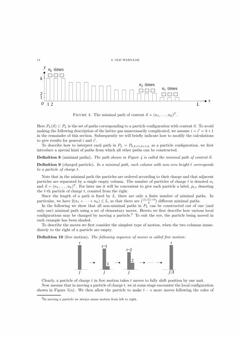
Figure 4. The minimal path of content ~n = (n1, . . . , nk)T .
Here PL(~n) ⊂ PL is the set of paths corresponding to a particle configuration with content ~n. To avoidmaking the following description of the lattice gas unnecessarily complicated, we assume i = i′ = k+1in the remainder of this section. Subsequently we will briefly indicate how to modify the calculationsto give results for general i and i′.
To describe how to interpret each path in PL = Pk,k+1,k+1;L as a particle configuration, we firstintroduce a special kind of paths from which all other paths can be constructed.
Definition 8 (minimal paths). The path shown in Figure 4 is called the minimal path of content ~n.
Definition 9 (charged particle). In a minimal path, each column with non-zero height t correspondsto a particle of charge t.
Note that in the minimal path the particles are ordered according to their charge and that adjacentparticles are separated by a single empty column. The number of particles of charge t is denoted nt
and ~n = (n1, . . . , nk)T . For later use it will be convenient to give each particle a label, pt,ℓ denotingthe ℓ-th particle of charge t, counted from the right.
Since the length of a path is fixed by L, there are only a finite number of minimal paths. In
particular, we have 2(n1 + · · · + nk) ≤ L, so that there are(
⌊L/2⌋+kk
)
different minimal paths.In the following we show that all non-minimal paths in PL can be constructed out of one (and
only one) minimal path using a set of elementary moves. Hereto we first describe how various localconfigurations may be changed by moving a particle.2 To suit the eye, the particle being moved ineach example has been shaded.
To describe the moves we first consider the simplest type of motion, when the two columns imme-diately to the right of a particle are empty.
Definition 10 (free motion). The following sequence of moves is called free motion:
j
t
j
t−1
1
j
t−2
2
j+1
t
Clearly, a particle of charge t in free motion takes t moves to fully shift position by one unit.Now assume that in moving a particle of charge t, we at some stage encounter the local configuration
shown in Figure 5(a). We then allow the particle to make t − s more moves following the rules of
2In moving a particle we always mean motion from left to right.
THE ANDREWS-GORDON IDENTITIES AND q-MULTINOMIAL COEFFICIENTS 15
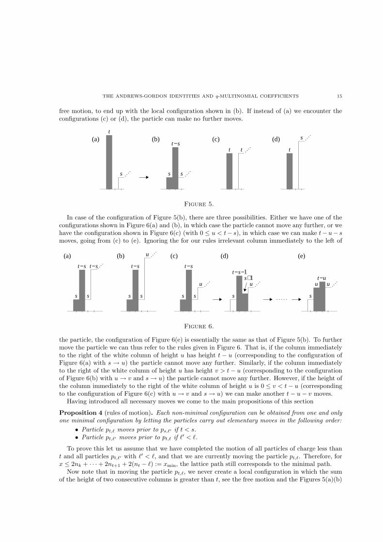
free motion, to end up with the local configuration shown in (b). If instead of (a) we encounter theconfigurations (c) or (d), the particle can make no further moves.
t
s s
t−s
s
t t t
s(a) (b) (c) (d)
Figure 5.
In case of the configuration of Figure 5(b), there are three possibilities. Either we have one of theconfigurations shown in Figure 6(a) and (b), in which case the particle cannot move any further, or wehave the configuration shown in Figure 6(c) (with 0 ≤ u < t− s), in which case we can make t− u− smoves, going from (c) to (e). Ignoring the for our rules irrelevant column immediately to the left of
s s
t−s t−s
s s
t−s
u
s s
u
t−s
s
u
t−s−1s+1
s
u ut−u
(a) (b) (c) (d) (e)
Figure 6.
the particle, the configuration of Figure 6(e) is essentially the same as that of Figure 5(b). To furthermove the particle we can thus refer to the rules given in Figure 6. That is, if the column immediatelyto the right of the white column of height u has height t − u (corresponding to the configuration ofFigure 6(a) with s → u) the particle cannot move any further. Similarly, if the column immediatelyto the right of the white column of height u has height v > t − u (corresponding to the configurationof Figure 6(b) with u → v and s → u) the particle cannot move any further. However, if the height ofthe column immediately to the right of the white column of height u is 0 ≤ v < t − u (correspondingto the configuration of Figure 6(c) with u → v and s → u) we can make another t − u − v moves.
Having introduced all necessary moves we come to the main propositions of this section
Proposition 4 (rules of motion). Each non-minimal configuration can be obtained from one and onlyone minimal configuration by letting the particles carry out elementary moves in the following order:
• Particle pt,ℓ moves prior to ps,ℓ′ if t < s.• Particle pt,ℓ′ moves prior to pt,ℓ if ℓ′ < ℓ.
To prove this let us assume that we have completed the motion of all particles of charge less thant and all particles pt,ℓ′ with ℓ′ < ℓ, and that we are currently moving the particle pt,ℓ. Therefore, forx ≤ 2nk + · · · + 2nt+1 + 2(nt − ℓ) := xmin, the lattice path still corresponds to the minimal path.
Now note that in moving the particle pt,ℓ, we never create a local configuration in which the sumof the height of two consecutive columns is greater than t, see the free motion and the Figures 5(a)(b)

16 S. OLE WARNAAR
012
k≤
1 2 Lx
y
Figure 7. The lattice path obtained from Figure 1 after moving the largest particlesto their minimal position. The shaded regions mark the three next-largest particles.
and 6(c)–(e). Since we have not moved any of the particles of charge greater than t, this means thatto the right of xmin no two consecutive columns have summed heights greater than t.3 Also note thatas soon as pt,ℓ meets two columns immediately to its right whose summed heights equal t, pt,ℓ cannotmove any further, see Figures 5(c) and 6(a). Consequently, pt,ℓ always corresponds to the leftmosttwo consecutive columns right of xmin whose summed height equals t. (In fact, it corresponds to theleftmost two consecutive columns right of xmin with maximal summed heights.)
Now we define reversed moves by reading all the previous figures in a mirror. Using this motionwe can move pt,ℓ all the way back to its minimal position but not any further. To see this we notethat the only situations in which pt,ℓ cannot be moved further back is if it meets two consecutivecolumns to its left whose summed heights are greater or equal to t. Since we have just argued thatsuch a configuration cannot occur between xmin and pt,ℓ we can indeed move pt,ℓ back to its minimalposition using the reversed moves. Once it is back in its minimal position we either have the mirrorimage of Figure 5(c) (in case ℓ < nt) or (d) (in case ℓ = nt). Neither of these configurations allowsfor further reversed moves.
The above, however, gives a general procedure for reducing each non-minimal path to a minimalone by simply reversing the rules of motion in the proposition. That is, we first scan the path forall particles of charge k, by locating all occurrence of two consecutive columns of summed heightsk. From left to right these label the particles pk,nk
to pk,1. Applying the previous reasoning witht = k, we can first move pk,nk
back using reversed moves, than pk,nk−1, et cetera, until all particles ofcharge k have taken their “minimal position”. Repeating this for the particles of charge k − 1, thenthe particles of charge k − 2, et cetera, each non-minimal path reduces to a unique minimal path.
As an example to the above, for the path of Figure 3 the shaded regions mark the (two) particleswith largest charge (=8). Moving them back using the reversed motion, the leftmost particle beingmoved first, we end up with the path shown in Figure 7, in which now the (three) particles withnext-largest charge have been marked. We leave it to the reader to further reduce the path to obtainthe minimal path of content (n1, n2, . . . , n8) = (2, 1, 2, 1, 3, 1, 3, 2).
The elementary moves and the reversed moves are clearly reversible. If a particle of charge t hasmade an elementary move changing a path from p to p′, we can always carry a reversed move goingfrom p′ back to p. Since each path can be reduced to a unique minimal path using the reversed movesby carrying out the rules of motion of proposition 4 in reversed order, we have thus established thatusing the rules of motion we can generate each non-minimal path uniquely from a minimal path.Hence the proposition is proven.
3 This also means that in moving a particle of charge t, the configurations of Figure 5(d) and Figure 6(b) in factnever arise.

THE ANDREWS-GORDON IDENTITIES AND q-MULTINOMIAL COEFFICIENTS 17
We now have established the decomposition of the sum (5.1) into (5.2), where ZL(~n; q) is thegenerating function of the paths generated by the minimal path labelled by ~n, or, in other words,ZL(~n; q) is the partition function of a lattice gas of fermions with particle content ~n. The fermionicnature being that, unlike particles of different charge, particles of equal charge cannot exchangeposition.
Our next result concerns the actual computation of the partition function.
Proposition 5. The partition function ZL is given by
(5.3) ZL(~n; q) = q ~nT C−1k ~n
k∏
t=1
[
nt + mt
nt
]
,
with ~m + ~n = 12 (Ik ~m + L~ek).
To prove this we first determine the contribution to ZL of the minimal path of content ~n,
W (pmin)/ ln q =k
∑
t=1
t
nt∑
ℓ=1
(
2ℓ − 1 + 2k
∑
s=t+1
ns
)
=k
∑
t=1
tnt
(
nt + 2k
∑
s=t+1
ns
)
(5.4)
=
k∑
r=1
k∑
t=r
nt
(
nt + 2
k∑
s=t+1
ns
)
=
k∑
r=1
N2r = ~nT C−1
k ~n.
To obtain the contribution to ZL of the non-minimal configurations, we apply the rules of motionof Proposition 4. If eℓ denotes the number of elementary moves carried out by pt,ℓ, the generatingfunction of moving the particles of charge t reads
(5.5)
mt∑
e1=0
e1∑
e2=0
. . .
ent−1∑
ent=0
qe1+e2+···+ent =
[
mt + nt
nt
]
.
Here we have used the fact that each elementary move generates a factor q and that pt,ℓ cannot carryout more elementary moves than pt,ℓ−1. (If pt,ℓ has made as many moves as pt,ℓ−1 we obtain eitherthe local configuration of Figure 5(c) or Figure 6a, prohibiting any further moves.) The number mt
in (5.5) is the maximal number of elementary moves pt,1 can make and remains to be determined. Ifthe content of the minimal path is ~n, the x-position of pt,1 in pmin is 2(nk + · · ·+ nt)− 1 := x0. To fixmt, let us assume that after the motion of the particles of charge less than t has been completed, thenontrivial part of the lattice path is encoded by the sequence of heights (fx0
, . . . , fL−1), with fx0= t,
fx0+1 = 0 and fj + fj+1 < t for j > x0. The particle pt,1 can now move all the way to x = L − 1making
mt = (t − fx0+2) + (t − fx0+2 − fx0+3) + (t − fx0+3 − fx0+4)
+ · · · + (t − fL−2 − fL−1) + (t − fL−1)
= t(L − x0 − 1) − 2
L−1∑
j=x0+2
fj(5.6)
elementary moves. To simplify this, note that the sum on the right-hand side is nothing but twice the
sum of the heights of the columns right of x = x0, which is 2∑t−1
s=1 sns. Substituting this in (5.6) andusing the definition of x0, results in
(5.7) mt = tL − 2
t−1∑
s=1
sns − 2t
k∑
s=t
nt = tL − 2
k∑
s=1
min(s, t)ns = L(C−1k )t,k − 2
k∑
s=1
(C−1k )t,sns
in accordance with Proposition 5.

18 S. OLE WARNAAR
01
i−1
k
1 2 Lx
y
nk times n i−1 times n1 times
Figure 8. The minimal path of content ~n = (n1, . . . , nk)T for general i. The dashedlines are drawn to mark the different particles.
Putting together the results (5.4), (5.5) and (5.7) completes the proof of Proposition 5. Substitutingthe form (5.3) of the partition function into (5.2) proves expression (1.8) of Theorem 5, for i = i′ =k + 1.
5.3. Fermi-gas partition function; general i and i′. Modifying the proof of Theorem 5 for i =i′ = k+1 to all i and i′ is straightforward and few details will be given. It is in fact interesting to notethat unlike our proof for the character identities of the unitary minimal models [44, 45], the generalcase here does not require the introduction of additional “boundary particles”.
First let us consider the general i′ case, with i = k + 1. This implies that the height fL−1
of the last column of the lattice paths is no longer free to take any of the values 1, . . . , k, but isbound by fL−1 ≤ i′ − 1. For the particles of charge less or equal to i′ − 1 this does not imposeany new restrictions on the maximal number of moves pt,1 can make. For t > i′ − 1 however, mt
in (5.7) has to be decreased by t − i′ + 1. Thus we find that mt of (5.7) has to be replaced bymt − max(0, t − i′ + 1) = mt − t + min(t, i′ − 1). Recalling (C−1
k )s,t = min(s, t), this yields
mt = (L − 1)(C−1k )t,k + (C−1
k )t,i′−1 − 2
k∑
s=1
(C−1k )t,sns
and therefore, mt + nt = 12 (
∑ks=1(Ik)t,sms + (L− 1)δt,k + δt,i′−1) which is in accordance with Propo-
sition 5, for i = k + 1.Second, consider i general, but i′ = k + 1, so that f1 ≤ i − 1, fL−1 ≤ k. Now the modification
is slightly more involved since the actual minimal paths change from those of Figure 4 to those ofFigure 8. This leads to a change in the calculation of W (pmin) to
W (pmin)/ ln q =
k∑
t=1
nt∑
ℓ=1
(
2ℓt − min(t, i − 1) + 2t
k∑
s=t+1
ns
)
=
k∑
t=1
tnt
(
nt + 2
k∑
s=t+1
ns
)
+
k∑
t=i
(t − i + 1)nt
= ~nT C−1k ~n +
k∑
t=1
tnt −k
∑
t=1
min(t, i − 1)nt = ~nT C−1k (~n + ek − ei−1),
which is indeed the general form of the quadratic exponent of q in (1.8). Also mt again requiresmodification, which is in fact similar to the previous case: mt → mt − max(0, t − i + 1). To see thisnote that it takes max(0, t− i+1) elementary moves to move pt,1 from its minimal position in Figure 4to its minimal position in Figure 8.
THE ANDREWS-GORDON IDENTITIES AND q-MULTINOMIAL COEFFICIENTS 19
Finally, combining the previous two cases, and using the fact that the modifications of mt due tof1 ≤ i− 1 and fL−1 ≤ i′ − 1 are independent, we immediately arrive at the general form of (1.8) with(m, n)-system (1.9).
6. Discussion
In this paper we have presented polynomial identities which arise from finitizing Gordon’s frequencypartitions. The bosonic side of the identities involves q-deformations of the coefficient of xa in theexpansion of (1 + x + · · ·+ xk)L. The fermionic side follows from interpreting the generating functionof the frequency partitions, as the grand-canonical partition function of a one-dimensional lattice gas.
Interestingly, in recent publications, Foda and Quano, and Kirillov, have given different polynomialidentities which imply (1.3) [22, 24, 32]. In the notation of Section 1 these identities can be expressedas
Theorem 7 (Foda–Quano, Kirillov). For all k ≥ 1, 1 ≤ i ≤ k + 1 and L ≥ k − i + 1,
(6.1)∑
n1,...,nk≥0
qN21+···+N2
k+Ni+···+Nk
k∏
j=1
[
L − Nj − Nj+1 − 2∑j−1
ℓ=1 Nℓ − αi,j
nj
]
=
∞∑
j=−∞
(−)jqj(
(2k+3)(j+1)−2i)
/2
[
L
⌊L−k+i−1−(2k+3)j2 ⌋
]
,
with Nk+1 = 0 and αi,j = max(0, j − i + 1).
An explanation for this different finitization of (1.3) can be found in a theorem due to Andrews [4]:
Theorem 8 (Andrews). Let Qk,i(n) be the number of partitions of n whose successive ranks lie inthe interval [2 − i, 2k − i + 1]. Then Qk,i(n) = Ak,i(n).
It turns out that it is the (natural) finitization of these successive rank partitions which gives rise tothe above alternative polynomial finitization. That is, (6.1) is an identity for the generating functionof partitions with largest part ≤ ⌊(L + k − i + 2)/2⌋, number of parts ≤ ⌊(L − k + i − 1)/2⌋, whosesuccessive ranks lie in the interval [2 − i, 2k − i + 1].
Let us now reexpress (6.1) into a form similar to equations (1.8), (1.12) and (1.13). Hereto weeliminate i in the right-hand side of (6.1) in favour of the variable s of equation (1.11) and split theresult into two cases. This gives
RHS(6.1) =
∞∑
j=−∞
{
qj(
(2j+1)(2k+3)−2s)
[
L12 (L + k − s + 1) + (2k + 3)j
](0)
1
−q
(
2j+1)(
(2k+3)j+s)
[
L12 (L + k + s + 1) + (2k + 3)j
](0)
1
}
for L + k even, and
RHS(6.1) =∞∑
j=−∞
{
qj(
(2j+1)(2k+3)−2s)
[
L12 (L − k + s − 2) − (2k + 3)j
](0)
1
−q
(
2j+1)(
(2k+3)j+s)
[
L12 (L − k − s − 2) − (2k + 3)j
](0)
1
}
for L + k odd. This we recognize to be exactly (1.12) and (1.13) with r = 0, kL replaced by L and[
...
...
](0)
kreplaced by
[
...
...
](0)
1.

20 S. OLE WARNAAR
Similarly, if we express the left-hand side of (6.1) through an (n, m)-system, we find precisely (1.8)but with
(6.2) ~m + ~n =1
2
(
Ik ~m + L~e1 +~ei−1 −~ek
)
.
This is just (1.9) with r = 0 and L ek replaced by L e1.From the above observations it does not require much insight to propose more general polynomial
identities which have (6.1) and those implied by the Theorems 5 and 6 as special cases. In particular,we have confirmed the following conjecture by extensive series expansions.
Conjecture 1. For all k ≥ 1, 1 ≤ ℓ ≤ k, 1 ≤ i ≤ k + 1, 1 ≤ i′ ≤ ℓ + 1 and ℓL ≥ k + ℓ − i − i′ + 2
∑
n1,n2,...,nk≥0
q ~nT C−1k (~n +~ek −~ei−1)
k∏
j=1
[
nj + mj
nj
]
with (m, n)-system given by
(6.3) ~m + ~n =1
2
(
Ik ~m + (L− 1)~eℓ +~ei−1 +~ei′−1 −~ek
)
equals
∞∑
j=−∞
{
qj(
(2j+1)(2k+3)−2s)
[
L12 (ℓL + k − s − r + 1) + (2k + 3)j
](r)
ℓ
−q
(
2j+1)(
(2k+3)j+s)
[
L12 (ℓL + k + s − r + 1) + (2k + 3)j
](r)
ℓ
}
for r ≡ ℓL + k (mod 2) and
∞∑
j=−∞
{
qj(
(2j+1)(2k+3)−2s)
[
L12 (ℓL − k + s − r − 2) − (2k + 3)j
](r)
ℓ
−q
(
2j+1)(
(2k+3)j+s)
[
L12 (ℓL − k − s − r − 2) − (2k + 3)j
](r)
ℓ
}
for r 6≡ ℓL + k (mod 2). Here s is defined as in (1.11) and
r = ℓ − i′ + 1
so that r = 0, . . . , ℓ.
For later reference, let us denote these more general polynomials as G(ℓ)k,i,i′ ;L(q). Then ℓ = k
corresponds to the polynomials considered in this paper and ℓ = 1 to those of Foda, Quano andKirillov.
The above conjecture leads one to wonder whether there are in fact (at least) k different partitiontheoretical interpretations of (1.3), each of which has a natural finitization corresponding to the
polynomials G(ℓ)k,i,i′ ;L(q) with ℓ = 1, . . . , k.
Intimately related to the conjecture and perhaps even more surprising is the following observation,originating from the work of Andrews and Baxter [10]. For k ≥ 0 and 1 ≤ i ≤ k+1, define a k-variablegenerating function
f(x1, . . . , xk) =∑
n1,n2,...,nk≥0
qN21+···+N2
k+Ni+···+Nk x2N1
1 x2(N1+N2)2 · · ·x
2(N1+···+Nk)k
(x1)n1+1(x2)n2+1 · · · (xk)nk+1,

THE ANDREWS-GORDON IDENTITIES AND q-MULTINOMIAL COEFFICIENTS 21
where (x)n =∏n−1
k=0 (1 − xqk). Obviously, (1 − x1) · · · (1 − xk)f(1, . . . , 1) corresponds to the left-
hand side of (1.3). Now define the polynomials P (ℓ1, . . . , ℓk) := P (~ℓ) as the coefficients in the seriesexpansion of f ,
f(x1, . . . , xk) =∑
ℓ1,...,ℓk
P (~ℓ)xℓ11 · · ·xℓk
k .
From the readily derived functional equations for f and the recurrences (4.1) with (4.3) one can deducethat
P (~m + 2C−1k ~n) = Gk,i,i′ ;L(q)
with ~m and ~n given by (1.9). Similarly the polynomials of Foda, Quano and Kirillov arise again asP (~m+2C−1
k ~n) where ~m and ~n now satisfy (6.2). Again we found numerically that also the polynomialsfeaturing the conjecture appear naturally. That is,
P (~m + 2C−1k ~n) = G
(ℓ)k,i,i′ ;L(q),
where now the generalized (m, n)-system (6.3) should hold (so that ~m + 2C−1k ~n = C−1
k ((L− 1)~eℓ +~ei−1 +~ei′−1 −~ek)).
Although all the polynomial identities implied by Conjecture 1 reduce to Andrews’ identity (1.3)in the L to infinity limit, they still provide a powerful tool for generating new q-series results. Thatis, if we first replace q → 1/q and then take L → ∞, new identities arise. To state these, we needsome more notation. The inverse Cartan matrix of the Lie algebra Aℓ−1 is denoted by Bℓ−1, and ~µand ~εj are (ℓ− 1)-dimensional (column) vectors with entries ~µj = µj and (~ǫj)m = δj,m. Furthermore,we need the k-dimensional vector
~Qi,i′,ℓ = ~ei +~ei+2 + · · · +~ei′ +~ei′+2 + · · · +~eℓ+1 +~eℓ+3 + · · · ,
with ~ej = ~0 for j ≥ k + 1. Using this notation, we are led to the following conjecture.
Conjecture 2. For all k ≥ 1, 1 ≤ ℓ ≤ k, 1 ≤ i ≤ k + 1, 1 ≤ i′ ≤ ℓ + 1 and |q| < 1, the q-series
(6.4) q(i′+i−2)/4∑
m1,m2,...,mk≥0
mj≡(~Qi,i′,ℓ)j (mod 2)
q
1
4~mT Ck(~m + 2~ek − 2~ei−1)
(q)mℓ
k∏
j=1j 6=ℓ
[ 12
(
Ik ~m +~ei−1 +~ei′−1 −~ek
)
mj
]
equals
(6.5) q(k+r−s+1)(k−r−s+1)/(4ℓ) 1
(q)∞
ℓ−1∑
n=0
∑
µ1,...,µℓ−1≥0
n+ℓ(Bℓ−1~µ)1≡0 (mod ℓ)
q ~µT Bℓ−1(~µ − ~ǫr)
(q)µ1· · · (q)µℓ−1
×
{ ∞∑
j=−∞
n+(k−s−r+1)/2+(2k+3)j≡0 (mod ℓ)
qj(
(2k−2ℓ+3)(2k+3)j+(2k+3)(k−ℓ+1)−(2k−2ℓ+3)s)
/ℓ
−
∞∑
j=−∞
n+(k+s−r+1)/2+(2k+3)j≡0 (mod ℓ)
q
(
(2k−2ℓ+3)j+(k−ℓ+1))(
(2k+3)j+s)
/ℓ
}

22 S. OLE WARNAAR
for r ≡ k (mod 2), and equals
(6.6) q(k+r−s+2)(k−r−s+2)/(4ℓ) 1
(q)∞
ℓ−1∑
n=0
∑
µ1,...,µℓ−1≥0
n+ℓ(Bℓ−1~µ)1≡0 (mod ℓ)
q ~µT Bℓ−1(~µ − ~ǫr)
(q)µ1· · · (q)µℓ−1
×
{ ∞∑
j=−∞
n−(k−s+r+2)/2−(2k+3)j≡0 (mod ℓ)
qj(
(2k−2ℓ+3)(2k+3)j+(2k+3)(k−ℓ+2)−(2k−2ℓ+3)s)
/ℓ
−
∞∑
j=−∞n−(k+s+r+2)/2−(2k+3)j≡0 (mod ℓ)
q
(
(2k−2ℓ+3)j+(k−ℓ+2))(
(2k+3)j+s)
/ℓ
}
for r 6≡ k (mod 2).
Since Conjecture 1 is proven for ℓ = 1 and k, we can for these particular values claim the aboveas theorem. In fact, for ℓ = 1, the above was first conjectured in [30] and proven in [25]. In [12, 28]
expressions for the branching functions of the (A(1)1 )M × (A
(1)1 )N/(A
(1)1 )M+N coset conformal field
theories were given similar to (6.5) and (6.6). This similarity suggests that (6.4), (6.5) and (6.6)
correspond to the branching functions of the coset (A(1)1 )ℓ × (A
(1)1 )k−ℓ−1/2/(A
(1)1 )k−1/2 of fractional
level.A very last comment we wish to make is that there exist other polynomial identities than those dis-
cussed in this paper which imply the Andrews–Gordon identity 1.3 and which involve the q-multinomialcoefficients.
Theorem 9. For all k ≤ 1 and 1 ≤ i ≤ k + 1,
(6.7)
L∑
a=0
{
L
a
}(k−i+1)
k
=
L∑
j=−L
(−)jqj(
(2k+3)(j+1)−2i)
/2 (q)L
(q)L−j(q)L+j.
Note that for i = k + 1 the left-hand side is the generating function of partitions with at most ksuccessive Durfee squares and with largest part ≤ L.
The proof of Theorem 9 follows readily using the Bailey lattice of [1]. For k = 1 (6.7) was firstobtained by Rogers [37]. For other k it is implicit in [1, 8].
Acknowledgements
I thank Anne Schilling for helpful and stimulating discussions on the q-multinomial coefficients.Especially her communication of equation (2.7) has been indispensable for proving Proposition 3. Ithank Alexander Berkovich for very constructive discussions on the nature of the fermi-gas of Section 4.I wish to thank Professor G. E. Andrews for drawing my attention to the relevance of equation (6)and Barry McCoy for electronic lectures on the history of the Rogers–Ramanujan identities. Finally,helpful and interesting discussions with Omar Foda and Peter Forrester are greatfully acknowledged.This work is supported by the Australian Research Council.
Appendix A. Proof of q-multinomial relations
In this section we prove the various claims concerning the q-multinomial coefficients made in Sec-tion 2.

THE ANDREWS-GORDON IDENTITIES AND q-MULTINOMIAL COEFFICIENTS 23
Let us start proving the symmetry properties (2.6) of Lemma 1. First we take the definition (2.4)and make the change variables jℓ → L − jk−ℓ+1 for all ℓ = 1, . . . , k. This changes the restriction onthe sum to j1 + · · · + jk = kL − a, changes the exponent of q to
(A.1)k−1∑
ℓ=1
(L − jk−ℓ)jk−ℓ+1 −k−1∑
ℓ=k−p
(L − jk−ℓ),
but leaves the product over the q-binomials invariant. We now perform a simple rewriting of (A.1) asfollows
(A.1) =
k−1∑
ℓ=1
(L − jℓ)jℓ+1 +
p∑
ℓ=1
jℓ − pL (by ℓ → k − ℓ)
=
k−1∑
ℓ=1
(L − jℓ)jℓ+1 −
k−1∑
ℓ=p
jℓ+1 + (k − p)L − a (by j1 + · · · + jk = kL − a),
which proves the first claim of the lemma. The second statement in the lemma follows for example,
by noting that[
La
](k)
k= q−a
[
La
](0)
k.
The proof of the tautologies (2.8) of Proposition 2 is somewhat more involved and we proceedinductively. For L = 0 (2.8) is obviously correct, thanks to
[
0
a
](p)
k
= δa,0.
Now assume (2.8) holds true for all L′ = 0, . . . , L. To show that this implies (2.8) for L′ = L + 1,we substitute the fundamental recurrence (2.7) into (2.8) with L replaced by L + 1. After somecancellation of terms and division by (1 − qL+1), this simplifies to
(A.2)
M∑
m=0
qmL
[
L
a − m
](m)
k
=
M∑
m=0
qmL
[
L
kL − a − m + M
](m)
k
,
where we have replaced k − p − 1 by M . Since in (2.8) we have p = −1, . . . , k − 1, (A.2) shouldhold for M = 0, . . . , k. A set of equations equivalent to this is obtained by taking (A.2)M=0 and(A.2)M − (A.2)M−1 for M = 1, . . . , k. In formula this new set of equations reads
M−1∑
m=0
qmL
{
[
L
kL − a − m + M − 1
](m)
k
− qL
[
L
kL − a − m + M − 1
](m+1)
k
}
=
[
L
kL − a + M
](0)
k
− qML
[
L
a − M
](M)
k
,
for M = 0, . . . , k. Now we use the induction assumption on the term within the curly braces, and thesecond symmetry relation of (2.6) on the first term of the right-hand side. This yields
M−1∑
m=0
qmL
{
[
L
a − M
](m)
k
− qL
[
L
a − M
](m+1)
k
}
=
[
L
a − M
](0)
k
− qML
[
L
a − M
](M)
k
.
Expanding the sum, all but two terms on the left-hand side cancel, yielding the right-hand side.Finally we have to show Equation (2.9) of Proposition 3 to be true. We approach this problem
indirectly and will in fact show that the right-hand side of (2.9) can be transformed into the right-handside of (2.7) by multiple application of the tautologies (2.8) and the symmetries (2.6). For the sakeof convenience, we restrict our attention to the case k and p even, and replace L in (2.7) and (2.9) by

24 S. OLE WARNAAR
L + 1. The other choices for the parity of k and p follow in analogous manner, and the details will beomitted.
Rewriting the right-hand side of (2.9) by replacing L by L + 1, using the even parity of k and p,and replacing p by k − M , gives
(A.3)
M∑
m=0m even
qmL
[
L
a − 12 (m + M)
](m)
k
+
M−1∑
m=1m odd
qmL
[
L
kL − a − 12 (m − M + 1)
](m)
k
+
k∑
m=M+2m even
q12
(
(2L+1)M−m)
[
L
a − 12 (m + M)
](m)
k
+
k−1∑
m=M+1
m odd
qk(L+1)+ 12
(
(2L+3)M−m+1)
−2a
[
L
k(L + 1) − a − 12 (m − M − 1)
](m)
k
.
The proof that this equals the right-hand side of (2.7) (with L replaced by L + 1 and p by k −M)breaks up into two independent steps, both of which will be given as a lemma. First, we have
Lemma 3. The top-line of equation (A.3) equals
(A.4)M∑
m=0
qmL
[
L
a − m
](m)
k
.
Second,
Lemma 4. The bottom-two lines of equation (A.3) equal
(A.5)
k∑
m=M+1
q(L+1)M−m
[
L
a − m
](m)
k
.
Clearly, application of these two lemmas immediately establishes the wanted result.At the core of the proof of both lemmas is yet another result, which can be stated as
Lemma 5. For M even and ℓ = 0, . . . , 12M , the following function is independent of ℓ:
Fℓ(M, a) =
M∑
m=M−ℓ
qmL
[
L
a − m
](m)
k
+
ℓ−1∑
m=0
qmL
[
L
kL − a − m + 12M − 1
](m)
k
+
M−ℓ−2∑
m=ℓ
m≡ℓ (mod 2)
qmL
{
[
L
a − 12 (m + M − ℓ)
](m)
k
+ qL
[
L
kL − a − 12 (m − M + ℓ) − 1
](m+1)
k
}
.
The proof of this is simple. First we apply the tautology (2.8) to the term within the curly braces,yielding
Fℓ(M, a) =M∑
m=M−ℓ
qmL
[
L
a − m
](m)
k
+ℓ−1∑
m=0
qmL
[
L
kL − a − m + 12M − 1
](m)
k
+
M−ℓ−2∑
m=ℓ
m≡ℓ (mod 2)
qmL
{
[
L
kL − a − 12 (m − M + ℓ) − 1
](m)
k
+ qL
[
L
a − 12 (m + M − ℓ)
](m+1)
k
}
.

THE ANDREWS-GORDON IDENTITIES AND q-MULTINOMIAL COEFFICIENTS 25
After separating the m = ℓ term in the first and the m = M − ℓ − 2 term in the second term withinthe curly braces, we change the summation variable m → m − 2 in the sum over the second termwithin the braces. This results in
Fℓ(M, a) =M∑
m=M−ℓ−1
qmL
[
L
a − m
](m)
k
+ℓ
∑
m=0
qmL
[
L
kL − a − m + 12M − 1
](m)
k
+
M−ℓ−3∑
m=ℓ+1
m≡ℓ+1 (mod 2)
qmL
{
[
L
a − 12 (m + M − ℓ − 1)
](m)
k
+ qL
[
L
kL − a − 12 (m − M + ℓ + 1) − 1
](m+1)
k
}
= Fℓ+1(M, a).
The proof of the Lemmas 3 and 4 readily follows from Lemma 5. To prove Lemma 3, note that thetop-line of (A.3) is nothing but F0(M). Since this is equal to F 1
2M (M), we get
(A.6) top-line of (A.3) =
M∑
m= 12M
qmL
[
L
a − m
](m)
k
+
12M−1∑
m=0
qmL
[
L
kL − a − m + 12M − 1
](m)
k
.
Applying equation (A.2) with M replaced by 12M − 1, to the the second sum, we simplify to equation
(A.4) thus proving our lemma.To prove Lemma 4, we apply the first symmetry relation of (2.6) to all q-multinomials in the
bottom-two lines of (A.3). After changing m → k − m in the second line and m → k − m − 1 in thethird line, the last two lines of (A.3) combine to
(A.7) fa
k−M−2∑
m=0m even
qmL
{
[
L
kL − a − 12 (m − M − k)
](m)
k
+ qL
[
L
a − 12 (m + M + k) − 1
](m+1)
k
}
,
with fa = q(L+1)M−a. This we recognize as
fa
{
F0(k − M, kL + k − a) − q(k−M)L
[
L
kL − a + M
](k−M)
k
}
.
Replacing the first term by F 12(k−M)(k − M, kL + k − a), gives
fa
12(k−M)−1
∑
m=0
qmL
[
L
a − 12 (M + k) − m − 1
](m)
k
+ fa
k−M−1∑
m= 12(k−M)
qmL
[
L
kL − a − m + k
](m)
k
.
Applying equation (A.2) with M replaced by 12 (k − M) − 1 and a by a − 1
2 (M + k) − 1, to the firstsum, this simplifies to
fa
k−M−1∑
m=0
qmL
[
L
kL − a − m + k
](m)
k
.
Finally using the symmetry (2.6), recalling the definition of fa and changing m → k − m, we getequation (A.5).
26 S. OLE WARNAAR
References
[1] A. K. Agarwal, G. E. Andrews and D. Bressoud, The Bailey lattice, J. Indian. Math. Soc. 51 (1987), 57–73.[2] H. L. Alder, Partition identities–from Euler to the present, Amer. Math. Monthly 76 (1969), 733–764.[3] G. E. Andrews, A polynomial identity which implies the Rogers–Ramanujan identities, Scripta Math. 28 (1970),
297–305.[4] G. E. Andrews, Sieves in the theory of partitions, Amer. J. Math. 94 (1972), 1214–1230.[5] G. E. Andrews, An analytic generalization of the Rogers–Ramanujan identities for odd moduli, Prod. Nat. Acad.
Sci. USA 71 (1974), 4082–4085.[6] G. E. Andrews, The Theory of Partitions (Addison-Wesley, Reading, Massachusetts, 1976).[7] G. E. Andrews, Partitions and Durfee dissection, Amer. J. Math. 101 (1979), 735–742.[8] G. E. Andrews, Multiple series Rogers–Ramanujan type identities, Pac. J. Math. 114 (1984), 267–283.[9] G. E. Andrews, Schur’s theorem, Capparelli’s conjecture and q-trinomial coefficients, Contemp. Math. 166 (1994),
141–154.[10] G. E. Andrews and R. J. Baxter, Lattice gas generalization of the hard hexagon model. III. q-trinomial coefficients,
J. Stat. Phys. 47 (1987), 297–330.[11] G. E. Andrews, R. J. Baxter and P. J. Forrester, Eight-vertex SOS model and generalized Rogers–Ramanujan-type
identities, J. Stat. Phys. 35 (1984), 193–266.[12] J. Bagger, D. Nemeshansky and S. Yankielowicz, Virasoro algebras with central charge c > 1, Phys. Rev. Lett. 60
(1988), 389–392.[13] R. J. Baxter, Rogers–Ramanujan identities in the hard hexagon model, J. Stat. Phys. 26 (1981), 427–452.[14] A. Berkovich, Fermionic counting of RSOS-states and Virasoro character formulas for the unitary minimal series
M(ν, ν + 1). Exact results, Nucl. Phys. B 431 (1994), 315–348.[15] A. Berkovich and B. M. McCoy, Continued fractions and fermionic representations for characters of M(p, p′)
minimal models, Lett. Math. Phys. 37 (1996), 49–66.[16] A. Berkovich and B. M. McCoy, Generalizations of the Andrews–Bressoud identities for the N = 1 superconformal
model SM(2, 2ν), Math. Comput. Modelling 26 (1997), 37–49.[17] A. Berkovich, B. M. McCoy and W. P. Orrick, Polynomial identities, indices, and duality for the N = 1 supercon-
formal model SM(2, 4ν), J. Stat. Phys. 83 (1996), 795–837.[18] D. Bressoud, Lattice paths and the Rogers–Ramanujan identities, Lecture Notes in Math. 1395 (1987), 140–172.
[19] S. Dasmahapatra, On the combinatorics of row and corner transfer matrices of the A(1)n−1 restricted face models,
Int. J. Mod. Phys. A 12 (1997), 3551–3586.[20] S. Dasmahapatra, R. Kedem, B. M. McCoy and E. Melzer, Virasoro characters from Bethe’s equations for the
critical ferromagnetic three-state Potts model, J. Stat. Phys. 74 (1994), 239–274.[21] E. Date, M. Jimbo, A. Kuniba, T. Miwa and M. Okado, Exactly solvable SOS models. Local height probabilities
and theta function identities, Nucl. Phys. B 290 [FS20] (1987), 231–273.[22] O. Foda, On a polynomial identity which implies the Gordon–Andrews identities: a bijective proof, preprint Uni-
versity of Melbourne No. 27-94.
[23] O. Foda, M. Okado and S. O. Warnaar, A proof of polynomial identities of type sl(n)1 ⊗ sl(n)1/sl(n)2, J. Math.Phys. 37 (1996), 965–986.
[24] O. Foda and Y.-H. Quano, Polynomial identities of the Rogers–Ramanujan type, Int. J. Mod. Phys. 10 (1995),2291–2315.
[25] O. Foda and Y.-H. Quano, Virasoro character identities from the Andrews–Bailey construction, Int. J. Mod. Phys.A 12 (1996), 1651–1675.
[26] O. Foda and S. O. Warnaar, A bijection which implies Melzer’s polynomial identities: the χ(p,p+1)1,1 case, Lett.
Math. Phys. 36 (1996), 145–155.[27] B. Gordon, A combinatorial generalization of the Rogers–Ramanujan identities, Amer. J. Math. 83 (1961), 393–
399.
[28] D. Kastor, E. Martinec and Z. Qiu, Current algebra and conformal discrete series, Phys. Lett. B 200 (1988),434–440.
[29] R. Kedem, T. R. Klassen, B. M. McCoy and E. Melzer, Fermionic quasiparticle representations for characters of
G(1)1 × G
(1)1 /G
(1)2 , Phys. Lett. B 304 (1993), 263–270.
[30] R. Kedem, T. R. Klassen, B. M. McCoy and E. Melzer, Fermionic sum representations for conformal field theorycharacters, Phys. Lett. B 307 (1993), 68–76.
[31] R. Kedem and B. M. McCoy, Construction of modular branching functions from Bethe’s equations in the 3-statePotts chain, J. Stat. Phys. 71 (1993), 865–901.
[32] A. N. Kirillov, Dilogarithm Identities, Prog. Theor. Phys. Suppl. 118 (1995), 61–142.

THE ANDREWS-GORDON IDENTITIES AND q-MULTINOMIAL COEFFICIENTS 27
[33] J. Lepowsky and M. Primc, Structure of the standard modules for the affine Lie algebra A(1)1 , Contemporary
Mathematics 46 (AMS, Providence, 1985).[34] E. Melzer, Fermionic character sums and the corner transfer matrix, Int. J. Mod. Phys. A 9 (1994), 1115–1136.[35] S. Ramanujan, Proof of certain identities in combinatory analysis, Proc. Cambridge Phil. Soc. 19 (1919), 214–216.[36] A. Rocha-Caridi, Vacuum vector representation of the Virasoro algebra, in: Vertex Operators in Mathematics and
Physics, eds. J. Lepowsky, S. Mandelstam and I. M. Singer (Springer, Berlin, 1985).[37] L. J. Rogers, Second memoir on the expansion of certain infinite products, Proc. London Math. Soc. 25 (1894),
318–343.[38] L. J. Rogers, On two theorems of combinatory analysis and some allied identities, Proc. London Math. Soc. (2)
16 (1917), 315–336.[39] L. J. Rogers, Proof of certain identities in combinatory analysis, Proc. Cambridge Phil. Soc. 19 (1919), 211–214.[40] M. Rosgen and R. Varnhagen, Steps towards lattice Virasoro algebras: su(1,1), Phys. Lett. B 350 (1995), 203–211.[41] A. Schilling, Polynomial fermionic forms for the branching functions of the rational coset conformal field theories
csu(2)M × csu(2)N /csu(2)N+M , Nucl. Phys. B 459 (1996), 393–436.[42] A. Schilling, Multinomials and polynomial bosonic forms for the branching functions of the csu(2)M ×
csu(2)N /csu(2)N+M conformal coset models, Nucl. Phys. B 467 (1996), 247–271.[43] I. J. Schur, Ein Beitrag zur additiven Zahlentheorie und zur Theorie der Kettenbruche, S.-B. Preuss. Akad. Wiss.
Phys.-Math. Kl. (1917), 302–321.[44] S. O. Warnaar, Fermionic solution of the Andrews-Baxter-Forrester model I: unification of CTM and TBA methods,
J. Stat. Phys. 82 (1996), 657–685.[45] S. O. Warnaar, Fermionic solution of the Andrews-Baxter-Forrester model II: proof of Melzer’s polynomial iden-
tities, J. Stat. Phys. 84 (1996), 49–83.[46] S. O. Warnaar and P. A. Pearce, Exceptional structure of the dilute A3 model: E8 and E7 Rogers–Ramanujan
identities, J. Phys. A: Math. Gen. 27 (1994), L891–L897.
Department of Mathematics, The University of Melbourne, VIC 3010, Australia