THE ANALYSIS ON TRADE EFFECT OF CHINA-

ASEAN FREE TRADE AGREEMENT—BASED ON

THE GRAVITY MODEL

BY

Jingya Zhou

Bachelor of Economics, Shandong University of Finance and Economics, 2014

A Report Submitted in Partial Fulfilment of the Requirements for the Degree of

Master of Arts

in the Graduate Academic Unit of Economics

Supervisor: Mehmet Dalkir, Ph D, Dept. of Economics

Examining Board: Herb Emery, PhD, Dept. of Economics

Murshed Chowdhury, PhD, Dept. of Economics

This report is accepted by the Dean of Graduate Studies

THE UNIVERSITY OF NEW BRUNSWICK

January, 2017

© Jingya Zhou, 2017

ii

Abstract

Globalization and regional integration are irreversible trends for the world

economy. Free trade agreements play crucial roles in promoting trade

liberalization and regional economic cooperation. In this report, the bilateral trade

between China and 16 trading partners is analyzed for the period 1998-2014.

Gravity model is used to reveal the economic effect of China-ASEAN free trade

agreement (CAFTA). Ordinary Least Squares (OLS) and Generalized Method of

Moments (GMM) estimation methods were applied in the analysis. The empirical

results showed that the trade effect of CAFTA was not obvious. China and

ASEAN members need to formulate further actions to facilitate bilateral trade.

iii

Acknowledgement

I would like to express my gratitude to my supervisor, Professor Mehmet Dalkir,

for his guidance, assistance and encouragement. I would also like to thank my

Examining Board, Herb Emery and Murshed Chowdhury, for their useful

comments on my report. Finally, thanks to my families members and my friends

for their support.

iv

Table of Contents

Abstract ...................................................................................................................... ii

Acknowledgement ..................................................................................................... iii

1. Introduction ............................................................................................................ 1

2. Literature review .................................................................................................... 3

3. Methodology and data .......................................................................................... 10

3.1 The Gravity model ...................................................................................... 10

3.2 The data ....................................................................................................... 13

3.3 Econometric specifications ......................................................................... 15

4. Results .................................................................................................................. 18

4.1 Graphical illustrations ................................................................................. 18

4.2 Empirical results ......................................................................................... 20

5. Conclusion............................................................................................................ 31

Reference .................................................................................................................. 34

Appendix .................................................................................................................. 39

Curriculum Vitae

1

1. Introduction

In the field of international trade, free trade agreements are often considered to

have a significant impact on bilateral trade. In this report, we studied the trade

effects of China and ASEAN Free Trade Agreement (CAFTA) during the period

from 1998 to 2014.

In November 2001, the idea of establishing China and ASEAN Free Trade

Agreements (CAFTA) is first proposed by the premier of China, and this idea was

supported by ASEAN leaders. In November 2002, “the Framework Agreement on

China-ASEAN Comprehensive Economic Cooperation” was signed by the leaders

of China and ASEAN member countries, which indicates CAFTA was officially

launched. In November 2004, "Agreement on Trade in Goods of CAFTA" was

signed by both parties, began to achieve comprehensive tariff reduction for all

parties. In January 2007, the two sides signed "Agreement on Trade in Service"

and this agreement came in to effect in July. In August 2009, the "Agreement on

Investment" was signed. In January 2010, CAFTA was fully adopted. China-

ASEAN Free Trade Area (CAFTA) is the first free trade area between China and

other countries, it is also the world's first regional economic cooperation with

developing countries, and it is one of the world's three major regional economic

cooperation organizations.

2

In this paper, we explored the trade effects of CAFTA on the basis of the gravity

model. Ordinary Least Squares (OLS) and Generalized Method of Moments

(GMM) were applied as econometric estimation methods. This report contains 4

sections: section1 reviews empirical studies of CAFTA in recent years and

determines gravity model as the theoretical basis of this thesis. Section 2 depicts

the gravity model, the data and methods of econometric estimation used in this

paper. Section 3 shows and explains the empirical results. Section 4 provides the

conclusion and policy recommendations.

3

2. Literature review

There are two methodologies widely used for the empirical study of the effects of

free trade agreements: Computable General Equilibrium (CGE) Model and the

Gravity Model.

Shudong (2010) employed the CGE Global Trade Analysis Project (GTAP) model

to analyze bilateral trade between China and other ASEAN members from 2001

to 2010. The simulation showed that CAFTA should have increased the member

countries’ GDP, welfare, and bilateral trade, while decreasing the trade flows with

Hongkong, Korea, Japan and India. Shudong (2010) suggests that “China could

give priority to increase production where it has comparative advantage, and

ASEAN members could shift resources from agricultural sector to industrial

sector.”

Jun and Chunlai (2008) studied the economic impact of fulfillment of CAFTA

over two stages: from 2002 to 2006 and from 2006 to 2010. Based on improved

GTAP model, Jun and Chunlai (2008) found that real GDP and social welfare had

a remarkable increase in both periods, particularly from 2006 to 2010. The author

also mentioned there is negative trade diversion between China and ASEAN

countries, but the trade creation is large enough to offset it.

4

Also using GTAP model, Yinhua and Mingtai (2005) simulate the bilateral trade

effect of China- Australia Free Trade Agreement by removing the border

protection and trade barriers. The authors find that real GDP and welfare

increases for both countries. Based on the empirical results, Yinhua and Mingtai

(2005) predict that the total volume of bilateral trade will increase by 5 billion

USD dollars and the bilateral investment will increase by 1 billion USD dollars in

2015. Furthermore, China and Australia should adjust the labor between sectors to

achieve better resources allocation.

From the perspective of ASEAN countries, Donghyun, Innwon, and Gemma

(2008) used a CGE model to examine the potential economic impact of CAFTA.

The empirical result shows that the trade between China and the ASEAN

countries is expected to increase by 32.5%, while trade among non-ASEAN

countries is expected to decrease by 3%. Specifically, the trade growth and

welfare gains are more obvious for relatively rich countries such as Malaysia,

Thailand and Singapore than poorer countries such as Cambodia and Myanmar.

Donghyun, Innwon, and Gemma (2008) also mentioned that “although CAFTA

tends to increase China’s trade, China’s major export markets will continue to be

the US, Hong Kong, Korea and Japan.”

Lee and Park (2005) use the gravity model to compare the trade effects of

possible free trade areas in East Asia, which includes Japan-Korea FTA, China-

5

Korea FTA, China-Korea-Japan FTA and China- Korea- Japan-ASEAN FTA.

They find that the trade effect of China-Korea-Japan-ASEAN Free Trade Area is

more obvious than other East Asian free trade areas, the results also shows that

there is no trade division in East Asian free trade areas.

Guihot (2010) applied the Gravity Model using panel data estimation to assess the

trade impact of free trade agreements over the period of 1985-2007, including

ASEAN free trade agreement, China-ASEAN free trade agreement and ASEAN-

South Korea free trade agreement. There are two conclusions based on the

estimates: (1) the ASEAN free trade agreement had positive impact on bilateral

trade. (2) China-ASEAN free trade agreement and ASEAN-South Korea

agreement was not beneficial for intra-regional trade.

Baier and Bergstrand (2007) use a panel dataset for 96 countries from 1960 to

2000 to study whether the free trade agreements could raise the volumes of

international trade. This paper use standard cross-sectional data models and panel

data methodologies to estimate the “average treatment effects” of FTAs on trade.

Based on empirical results of gravity function, they find the cross-sectional

techniques tend to be biased, and the model using panel data with fix-effect

estimation after first-differencing could solve the problem of endogeneity.

Furthermore, by adding lagged terms of FTA dummy variables into the equation,

6

the estimates show that free trade agreements will increase the bilateral trade by

114% after 10 years.

Based on the study of Baier and Bergstrand (2007), Fan (2013) used a dynamic

panel approach in the analysis of China- ASEAN free trade area. Fan (2013)

suggests that the formation of China-ASEAN free trade agreement will increase

the volume of trade between China and ASEAN countries by 158% after 4 years,

this estimate is about 1.3 times the estimation of Baier and Bergstrand (2007).

In order to compare imports and exports between China and ASEAN countries,

Wen (2009) set up a gravity model. With a panel dataset, which includes 133

trade partners of China during the period of 2002-2006, the author indicates that

the formation of China-ASEAN free trade zone facilitates the exports and imports

between China and ASEAN countries, but the coefficients of FTA dummy

variables become smaller in the export model, which suggests the promoting

effect of CAFTA on exports is weakening.

Peter (2000) introduced a new index to the gravity model. This index is used to

measure the relative size of two economies in terms of GDP, the larger the value

of the index means the more similar their economies of scale and the higher the

volumes of interindustry trade. Fixed effects and random effects were applied to

this research. Peter (2000) also discussed that the panel approach is better than

cross-section techniques: “it allows disentangling time invariant country-specific

7

effects and capturing the relationships between the relevant variables over a

longer period.”

Following the path of Peter (2000), Lin (2011) applied the relative country size

index to analyze trade effects of China-ASEAN FTA. The result suggests that

China and ASEAN countries have different economies of scale and

underdeveloped intra-industry trade. The result also shows that coefficient of the

FTA dummy variable is negative, which means that bilateral trade between China

and one other country is not beneficial if this country is a member country of

CAFTA.

Yeqing (2015) introduced the economic gap and foreign direct investment to the

gravity model. The author concluded that the economic gap and foreign direct

investment had a positive impact on bilateral trade between China and ASEAN

countries. A 1% increase in foreign direct investment (from ASEAN countries to

China) will increase bilateral trade between China and ASEAN countries by

0.06%. The coefficient of FTA dummy variables also shows that the formation of

CAFTA actually promotes the bilateral trade between China and ASEAN

countries.

Benjamin (2003) considers common border effect and the trade relation within

other free trade agreements (European Union FTA and North American FTA) as

factors to study the feasibility of China- ASEAN FTA. The author states that

8

NAFTA and EU have positive impact on the trade flows within CAFTA, although

the bilateral trade between CAFTA and EU is declining. The OLS estimation also

shows that border effects are not beneficial to facilitate trade flows between China

and ASEAN countries. Benjamin (2003) applied RCAI (Revealed Comparative

Advantage Index) to measure the degree of competitiveness in production

between China and ASEAN countries. His results indicate that the products of

China and ASEAN countries are not complementary.

Compared with these literature above, there are some differences in this research:

(1) the literatures we talked before applied econometric method OLS, Fixed-

effects and Random-effects to estimate the trade effects of CAFTA, this paper

used OLS and GMM estimation to run the regression respectively and found that

GMM estimator is better. (2) The latest study is from Yeqing (2015), this author

explored of bilateral trade effects of CAFTA by 2012, the time range of this

report is from 1998 to 2014, this is the newest data we could find. (3) This report

introduced exchange rate and the wolrd oil price as explanatory variables to the

analysis.

Although the trade effect of CAFTA can be analyzed from the perspectives of

both the gravity and the CGE models, there is a large difference between these

two methodologies. Olena and Aaron (2007) argued that the CGE model is

commonly used to forecast the potential impact of the latest trade policy while the

9

gravity model focuses on ex-post impact. The CGE model can be used for

quantitative estimations of effects of trade on welfare allocation and revenue

streams. Compared to that, the gravity model provides the bilateral trade impacts.

The target of this paper is to analyze the effect of CAFTA on trade. The gravity

model is the choice model for analysis.

10

3. Methodology and data

3.1 The Gravity model

Inspired by Newton’s law, Tinbergen (1962) and Poyhonen (1963) first applied

the law of gravity to international trade, for the purpose of examining the impact

of economic size (Yi and Yj) and distance (Dij) on bilateral trade (Tij). The

original form is,

Tij=A（Yi Yj/Dij），A constant. (1)

Brada and Méndez (1985) introduced FTA dummy variable (Pij) into the gravity

model, to analyze the bilateral trade effects with or without free trade agreement.

The basic model is:

Tij=α0Yiα1Yj

α2Dijα3Pij

α4， (2)

Typically, we transform the basic function to the log-linear form:

ln Tij=lnα0 +α1lnYi +α2lnYj +α3ln Dij+α4ln Pij+εij (3)

lnα0 is the constant , εij is the error term, and Pij>0,

In the subsequent study, Frankel and Stein (1994) introduced common language,

transportation costs and tariff variables to the gravity function. Mc Callum (1995)

considered border effect as influential factors of bilateral trade. Benjamin (2003)

applied the trade relation with other free trade areas into the study of the gravity

11

model. At the same time, there were economists committed to find the economic

foundation of the gravity model. Among those, Krugman (1985) derived the

gravity model from Heckscher-Ohlin model. Keller (1998) proposed that the

Ricardian framework provided the theoretical basis for the gravity model.

This paper will introduce foreign direct investment, free trade agreement, oil price,

exchange rate, dummy variable year2002, and year2009 as explanatory variables.

Besides ASEAN countries, we include China’s top10 main trade partners

(Australia, Japan, Korea, United States, Hongkong, Canada, France, Brazil,

Germany and India) into our sample, in order to be able to compare the results

from trade between CAFTA member countries versus non-CAFTA member

countries. Furthermore, we will divide the total bilateral trade into two parts:

imports and exports, due to the great difference between import volume and

export volume for China and ASEAN countries. The export model and the import

model are specified as:

lnEXict=β0+β1ln(gdpctgdpit)+β2lndistanceic+β3lnfdiict+β4ASEANi+β5oilpricet+β

6 exchangeratet+β7year2002+β8year2009+ uic (5)

lnIMict=α0+α1ln(gdpctgdpit)+α2lndistanceict+α3lnfdiict+α4ASEANi+α5oilpricet+

α6exchangeratet +α7year2002+α8year2009+eic (6)

Where:

12

c indicates China, i indicates Cambodia, Singapore, Thailand, Malaysia,

Philippines, Indonesia, Australia, Japan, Korea, united states, Hongkong ,

Canada ,France, Brazil, Germany or India.

EXic : exports from China to country i in year t

IM ic: Chinese imports from country i in year t

gdpct: China’s Gross Domestic Product per capita in year t

gdpit: country i’s Gross Domestic Product per capita in year t

distanceic: the straight distance between the capital cities of country c and country

i

lnfdiict: foreign direct investments from country i to China

Exchangeratet: exchange rate between China and U.S.(direct quotation)

ASEANi: dummy variable for China- ASEAN free trade agreement

year2002: year dummy variable for China- ASEAN free trade agreement was

signed in 2002

year2009: year dummy variable for global financial crisis

oilpricet: the world price of crude oil in year t

uic ,eic: error terms

13

β0，α0 : Constants

α1,α2,α3,α4,α5,α6, β1,β2,β3,β4,β5,β6 are parameters

3.2 The data

This paper studies the bilateral trade between China and 16 countries over the

period of 1998 -2014, which is a strong-balanced panel dataset. According to

‘China statistical yearbook 2015’, we selected China’s principle trading partners

in 2014 (TOP10) and six ASEAN countries as our research object. Top 10

bilateral trade partners contains Australia, Japan, Korea, United States,

Hongkong , Canada , France, Brazil, Germany and India. ASEAN6 includes

Malaysia, Thailand, Singapore, Philippines, Indonesia and Cambodia.

Although Myanmar, Laos, Vietnam, Brunei Darussalam are ASEAN members,

some data for these countries are missing during 1998-2014: foreign direct

investment data of Laos, Vietnam, and Brunei Darussalam are not available; the

gross domestic product per capita data of Myanmar is missing from 2005 to 2011.

Besides, during the period 1998-2014, total volume of bilateral trade between

China and ASEAN6 accounts for more than 86% 1of the trade between China and

all ASEAN member countries. For the reasons above, we included ASEAN6

1 The data from National Bureau of Statistics of China

14

rather than all ASEAN member countries in our analysis. Since we discussed the

bilateral trade between China and 16 trading partners, there are 16 groups and a

total of 272 observations in this paper.

The export, import, exchange rate and foreign direct investment data used in this

paper are from national bureau of statistics of China. The gross domestic product

per capita and the world oil price data is collected from the World Bank. The

distance data is from the online distance calculator2, which refers to the straight

distance between capital cities. In order to exclude the effect of inflation, we use

real GDP per capita and real price of crude oil.

The world oil price variable is taken as a proxy variable for transportation costs,

which is often considered to have an important impact on bilateral trade. Noted

that the price of crude oil captures the endogenous effect on production and

indirect impact on real GDP.

Exchange rate fluctuations always have a crucial role to play in affecting import

and export. In order to simplify the measurement of exchange rate, exchange rate

between China and U.S. is introduced in this paper, from the direct quotation

method.

For the purpose of comparing the difference of CAFTA member countries to non-

CAFTA member countries, we used a dummy variable named “ASEAN. If

2 distance calculator : http://www.indo.com/distance/

15

country i is a CAFTA member country, ASEAN is set to 1; if not, ASEAN is set

to 0.

Since China- ASEAN Free Trade Agreement was signed in November 4, 2002,

we included an FTA dummy variable: if the year is between 1998 and 2002, the

variable takes the value 0; for the years after 2002, the FTA dummy variable takes

the value 1. We use this dummy variable to capture the differences of imports and

exports before and after the CAFTA was signed. The other year dummy variable

is year2009, which is a turning point for CAFTA, this variable marks the impacts

of global financial crisis on the bilateral trade of China and other 16 countries.

The dummy variable takes 1 when the year after 2009, is otherwise 0.

3.3 Econometric specifications

We applied two approaches: Ordinary Least Square (OLS) and the Generalized

Method of Moments (GMM) to estimate the equation (5) and equation (6),

respectively.

3.3.1 OLS estimation

OLS is a frequently used method to estimate the gravity model However, some

economists argued that there are some limitations of OLS estimation. Hanh (2009)

stated that OLS results may face the challenge of inconsistent and biased

estimates. Matthias and Jens (2012) found that “OLS and within group

16

approaches may yield biased estimations, instrumental variables are needed to

deal with the problem”.

3.3.2 GMM estimation

To overcome the drawbacks of OLS estimation, we adopted the GMM approach.

Arellano and Bond (1991) developed Generalized Method of Moments (GMM)

framework to estimate a dynamic panel model. Arellano and Bond (1991) also

tested the performance of GMM with Monte Carlo simulation and found that

GMM has negligible bias, substantially small variances and high efficiency.

The GMM estimator takes the first differenced regression equation and uses the

lagged levels of dependent and explanatory variables as instruments to eliminate

the unobserved effects. As Hanh (2009) mentioned, GMM estimator is capable of

reducing the bias and resolving the problem of endogeneity.

In this paper, estimation refers to the method that we used to run the regression,

such as OLS and GMM. Estimator indicates the rule that we used to yield

regression results. Estimate means the expected value from the calculation of

estimator.

Note that we applied the GMM estimation based on the gravity model at the

starting point, after using the first difference of GMM estimation, the distance will

17

not be in the model, thus the theoretical model is no more the gravity model in

first differenced GMM estimation.

18

4. Results

4.1 Graphical illustrations

4.1 graphical illustrations

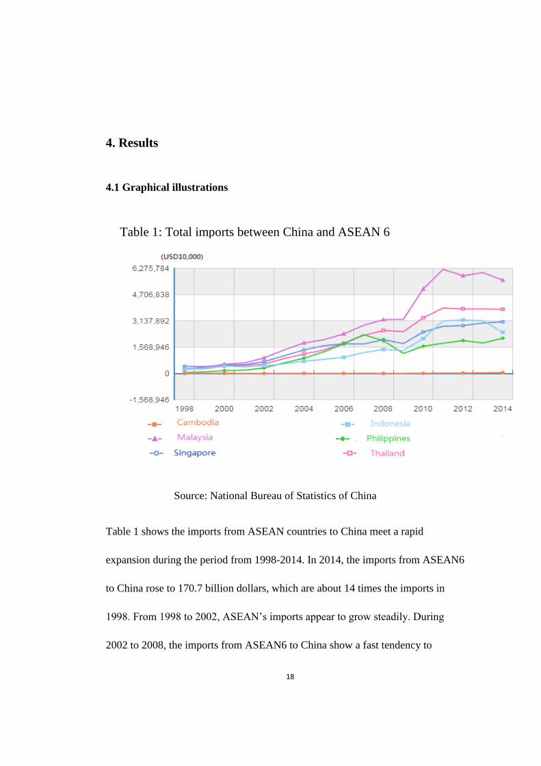
Source: National Bureau of Statistics of China

Table 1 shows the imports from ASEAN countries to China meet a rapid

expansion during the period from 1998-2014. In 2014, the imports from ASEAN6

to China rose to 170.7 billion dollars, which are about 14 times the imports in

1998. From 1998 to 2002, ASEAN’s imports appear to grow steadily. During

2002 to 2008, the imports from ASEAN6 to China show a fast tendency to

Table 1: Total imports between China and ASEAN 6

19

increase, the imports from 296 billion dollars increased to 111.7 billion dollars.

Due to the world financial crisis, the total values of imports was declining in 2009.

After 2009, the imports rise during 2010 and 2011. From 2011 to 2014, growth

rate of total imports decreased gradually from 1.6% to -0.4%.

Table 2 : total exports between China and ASEAN6

Source: National Bureau of Statistics of China

Analogous to imports, Table 2 also shows that there is an upward trend for total

exports from China to ASEAN 6 over the period 1998-2014. From 1998 to 2002,

the total exports show a slow growth. During the period 2002-2008, the ASEAN’s

exports increased sharply from 20.6 billion dollars to 96.8 billion dollars. Due to

the world financial crisis, the total value of exports was falling down in 2009.

20

After 2009, the exports from China to ASEAN 6 grew sharply. The average

growth rate is 20.9% for 2010-2012. For the period from 2013 to 2014, the

growth of exports started to slow down. In 2014, the growth rate of exports is

close to 5%.

4.2 Empirical results

4.2.1 First differenced OLS results

Table 3 and Table 4 show that the unit root test and autocorrelation test for OLS

estimation (without first differencing). The result of Augmented Dickey-Fuller

test (see Table3) indicates that the data series used did not contain unit root at a 10

percent significance level. The Durbin-Watson test (see table 4) shows there is

positive autocorrelation between error terms. In order to deal with the

autocorrelation problem, first differencing method is used. It should be noted that

the first- differencing method were used to the full equation except the dummy

variables.

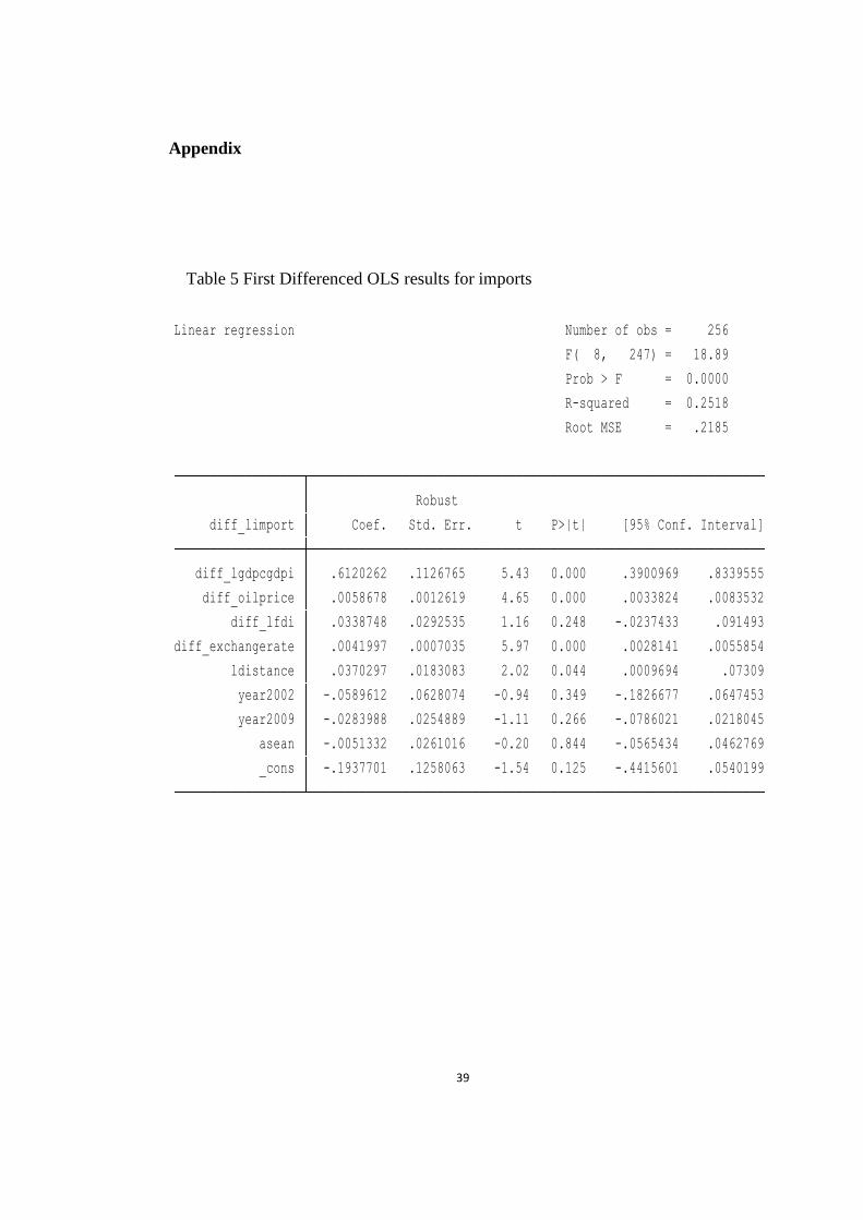
Table 5 (see Appendix) shows the first differenced OLS results for the model for

imports. The F- test shows that the model is statistically significant. The adjusted

R-square is 0.25, which means the independent variables can explain 25% of the

variance in total imports. Except for coefficients of ‘ASEAN’, foreign direct

investment, year2002, year2009 are not statistically significant, all other

coefficients of variables are statistically significant at 5 percent level. The

21

coefficient of the multiplication of two country’s GDP indicates that 1% increase

in GDP for either of two countries will lead to 0.61% increase in the growth rate

of total volumes of imports, by holding other variables constant. The estimate of

the coefficient of oil price is 0.006, which means keeping other variables constant,

when the world oil price increased by 1 dollar, the the growth rate of total imports

will increase by 0.6 percent. The sign of the estimates exchange rate is positive,

which indicates the the growth rate of volume of import will increase as exchange

rate increases. This result is weird since the depreciation in currency would be

expected to be correlated with declining imports. Kamada (2005), Willem (2012)

also found that the depreciation of RMB has positive effect on import. Willem

(2012) pointed out that this is because “the depreciation of the RMB will increase

exports, and will also increase imports that are used for re-export at the same

time”. The coefficient of distance is 0.004, which means the distance is positively

proportional to the imports. This coefficient is not according to our expectation.

In ur analysis, we considered China’s top10 primary trading partners. Table 1

shows that Chinese imports from ASEAN members has a upward trend, compared

to The United States, Germany, Australia and other primary trading partners, the

imports from ASEAN to China were not considerable(see table 6), which may

explain why the imports have positive relation with distance. However, another

fact is that Table 6 also showed that neighbor countries Japan and Korea occupied

22

large share in Chinese import market from 1998 to 2014. This result is anomaly

and it could be a question for future research.

Table 7 (see Appendix) shows the first differenced OLS results for the export

model. The F-test indicates that the model is statistically significant. The R-square

is 0.24, which means the explanatory variables can explain 24% of the total

volume of exports. In addition to the estimates of distance, year2002 and ASEAN

variables are not statistically significant, all other variables are statistically

significant at 10 percent level. The coefficient of the multiplication of GDPc and

GDPi suggests that if there is 1% increase in either the GDP of China or country i,

the growth rate of exports between China and country i will increase by 0.67%.

The estimates of foreign direct investment is 0.06, which states that 1 percent

increase in the foreign direct investment will lead to 0.06 percent increase in the

growth rate of total value of exports. The sign of the coefficient of exchange rate

is positive, which means the growth rate of exports will increase as the exchange

rate increases, it satisfies the economic condition, and since currency depreciation

could stimulate the volume of export. The estimates of dummy variable

‘Year2009’ is -0.07, which indicates that the growth rate of exports decreased by

7 percent after 2009. Due to the global financial crisis, this estimate is

understandable. The coefficient of distance shows that there is positive relation

between distance and total values of exports. The estimates of the coefficient of

oil price is 0.005, which means if the world oil price increase by 1 percent, the

23

growth rate of exports from China to trading partners will decrease by 0.5 percent.

This is an unusual result for oil price, which could be explained by the export

structure of China, China is a labor-intensive exporter rather than a energy-

intensive exporter, thus the increasing price of crude oil just have a slight impact

on China’s exports.

24

Table 3 Augmented Dickey-Fuller test for unit root for OLS estimation

variable Test statistic 5%critical value p-value

Ln(Import) -4.519 -2.879 0.0002

Ln(Export) -4.471 -2.879 0.0002

Ln(GDPcGDPi) -4.282 -2.879 0.0005

Ln(FDI) -2.693 -2.879 0.0753

Oilprice -7.910 -2.879 0.0000

Exchange rate -10.009 -2.879 0.0000

Table4 Durbin-Watson test for residual autocorrealtions for OLS estimation

MODEL d-statistic dl du

IMPORT MODEL 0.201 1.592 1.768

EXPORT MODEL 0.567 1.592 1.768

25

Cambodia0%

Indonesia3%

Malaysia6%

Philippines2%

Singapore3% Thailand

4%

Canada2%

United States14%

Germany9%

France2%

Brazil4%

Austrilia7%

Hongkong2%

India2%

Japan22%

Korea18%

Table 6:total values of imports during 1998-2014

26

4.2.2 first-differenced GMM result

Because of the problem of omitted variables, there is an autocorrelation in the

OLS estimation. Thus we applied GMM estimation to address this issue. After the

GMM estimation with log-levels, the Arellano-Bond test and Levin-Lin-Chu test

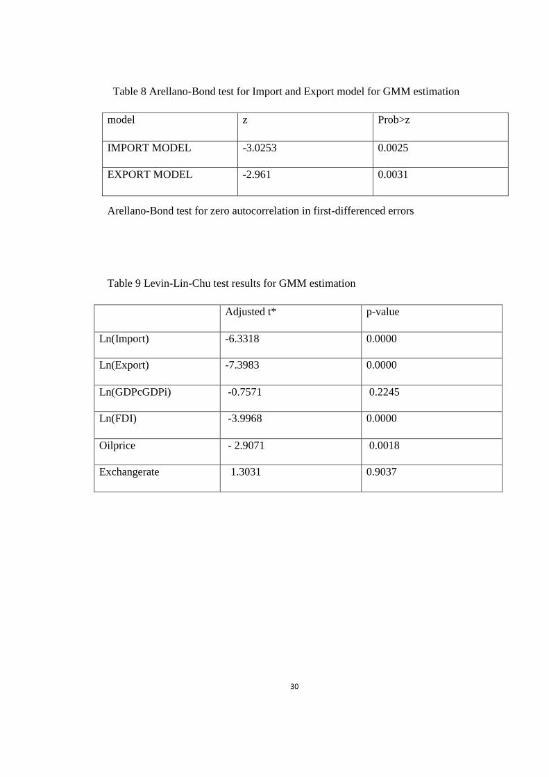
are used to identify if there are problems of autocorrelation and unit root. Table 8

shows the autocorrelation did not exist in import model at 5 percent significant

level, and there are no autocorrelation in export model at 5 percent level. Table 9

shows the Levin-Lin-Chu results. The results indicate that the panel model

contains unit roots. In order to remove the unit roots and possibilities of

autocorrelations, we took the first difference of the explanatory variables based on

the GMM estimation. It should be noted that the first- differencing method were

used to the full equation except the dummy variables

An important detail to mention is that the previous GMM estimation is based on

the gravity model, but after we took the first-differencing of GMM estimation, the

theoretical model is no more a gravity model, it turned into the reduced form

model.

Table 10 (see Appendix) shows the GMM result with first differencing for import.

In this regression, except the coefficients for FDI , year2002,the lag level of GDPs

and exchange rate, all other estimates are statistically significant at 5 percent level.

The contemporary coefficient on oil price is positive while the lagged coefficient

27

of oil price is negative, so we calculate the sum of these two coefficients, it is

negative, which reveals that the world oil price is negatively correlated with the

growth rate of total value of imports. The contemporary coefficient of the

multiplication of GDPs is 0.57, while the lag coefficient of GDP variable is -0.16,

the sum of coefficients is 0.41, which shows although the contribution of GDP to

the growth of exports is fluctuating, GDP still have positive impact on the growth

rate of total exports as a whole. The sum of coefficients of exchange rate is

positive, which means exchange rate is positively related to growth rate of import,

this abnormal result we explained before in 4.2.1. The estimate of time dummy

variable ‘year2002’ is insignificant. The coefficient of ‘year2009’ is negative and

significant, which means after 2009, the growth rate of total imports is turning

down. Distance carries a positive coefficient and significant at 1 percent level.

This indicates that when the distance increases by 1% the imports will increase by

1%. In the empirical study of distance, many researchers used the square of

distance. In this paper, the GMM estimation used log levels, thus it is reasonable

to use the actual value of distance through the estimation. The coefficient of FDI

is not statistically significant, which means that the foreign direct investment did

not provide the beneficiary effects on total volume of imports.

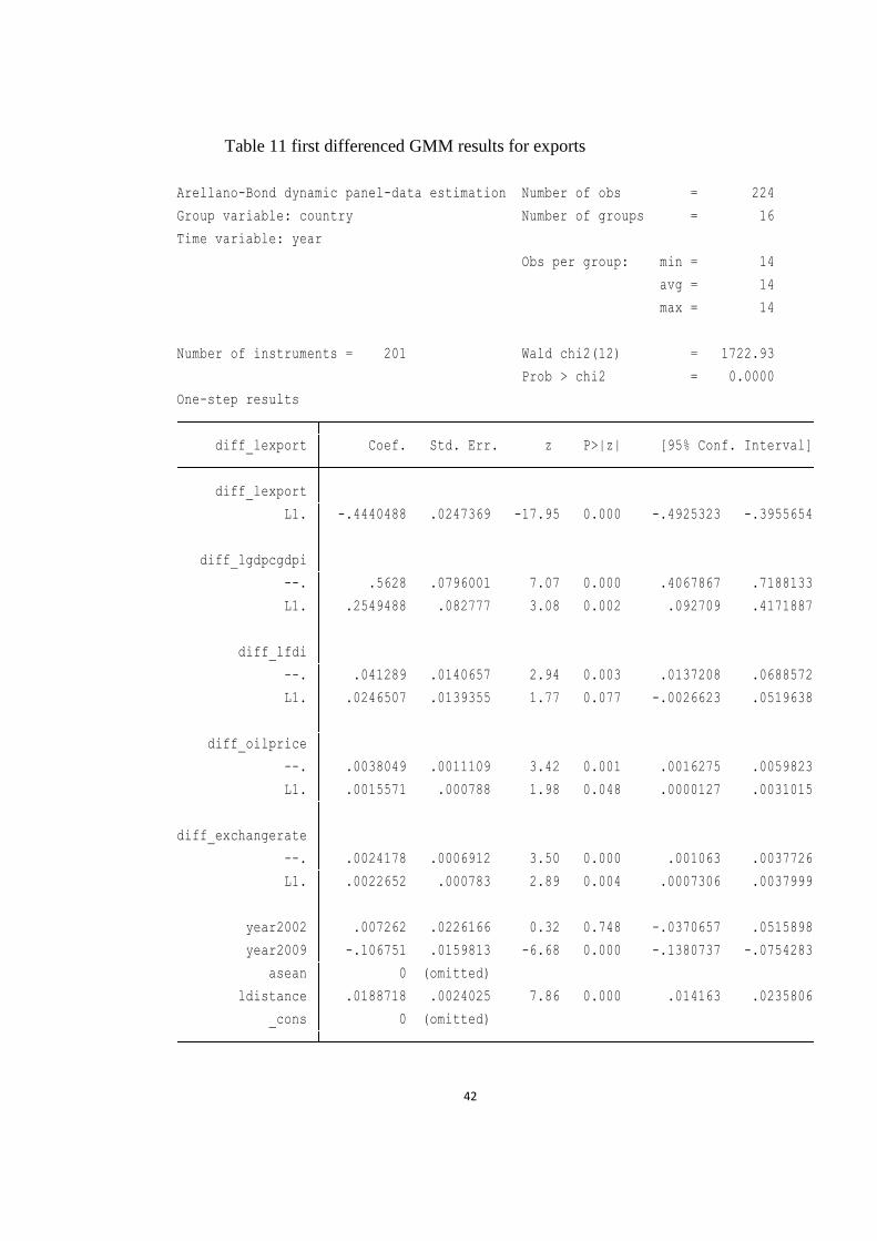
Table 11 (see Appendix) report results of first differenced GMM estimation for

export model. In this regression, except for the dummy variable ‘year2002’, all

other coefficients are statistically significant at 10 percent level. Both of the

28

coefficient on contemporaneous GDP and lagged GDP variable have positive

signs, the sum of GDP coefficients is 0.81, which indicates that GDP have

positive effects on growth rate of total imports. The estimate of FDI variable is

0.04 and statistically significant at 1percent level, which indicates 1% increase in

FDI from trading partners to China will increase the growth rate of bilateral

export by 0.04%. The coefficient FDIt-1 is 0.025, which means that the FDI still

have positive and significant impact on exports with one year lag. Both of the

contemporary and lag coefficients of “oilprice” are positive. This can be

explained by the export structure of China, which we discussed before. The

coefficients of exchange rate are positive in contemporaneous level and lagged

level. As we can see, the exchange rate contributes positive impacts on imports

and exports. According o the common sense, the increase of exchange rate will

increase exports and decrease exports. This could be explained by the exchange

rate policy of China. The exchange rate regime in China is the peg exchange rate

system, it is a combination of floating exchange rate system and fixed exchange

rate system. As the government is able to manage the value of RMB, so it is no

surprise to observe the abnormal results for exchange rate. The coefficient

“ASEAN” is omitted, which means no matter whether the country is a member of

CAFTA, it has nothing to do with the total exports. The coefficient of year2009 is

negative and significant, which means the growth rate of total exports is

29

decreasing after 2009, which could be explained by the effect of the global

financial crisis.

30

Table 8 Arellano-Bond test for Import and Export model for GMM estimation

model z Prob>z

IMPORT MODEL -3.0253 0.0025

EXPORT MODEL -2.961 0.0031

Arellano-Bond test for zero autocorrelation in first-differenced errors

Table 9 Levin-Lin-Chu test results for GMM estimation

Adjusted t* p-value

Ln(Import) -6.3318 0.0000

Ln(Export) -7.3983 0.0000

Ln(GDPcGDPi) -0.7571 0.2245

Ln(FDI) -3.9968 0.0000

Oilprice - 2.9071 0.0018

Exchangerate 1.3031 0.9037

31

5. Conclusion

This paper aims to reveal the economic effect of China-ASEAN Free trade

agreement. The panel gravity model covers 16 countries’ trade dataset (ASEAN6

and China’s top10 trading partners) over the period of 1998-2014. OLS and

GMM methodologies are used to estimate the effects of CAFTA.

The empirical results based on first differenced OLS and GMM estimation are not

in complete agreement. For import model, in the both of first differenced OLS

and GMM estimation, one can see GDP variable contributes significant impact on

total value of imports, geographic distance carries positive correlation with

imports, and the rise of exchange rate facilitates the volume of import. Foreign

direct investment is not statistically significant in neither of first differenced OLS

and GMM estimations for import. In addition, there is one variable have

unexpected estimates. The coefficient of world oil price has a positive relationship

with import in first differenced OLS estimation, while the first differenced GMM

estimation shows there is a negative correlation between oil price and import..

Based on the analysis above, first differenced GMM estimation is a better choice

because it has higher significance levels.

For export model, based on the empirical results of both first differenced OLS and

GMM estimation, we can conclude that GDP and Foreign direct investment have

positive effects on total volume of exports, there is a negative relationship

32

between the world oil price and exports, the rise of exchange rate will stimulates

the growth of export, the estimates of ‘year 2009’ shows that the world financial

crisis affect bilateral exports passively. The FTA dummy variable ‘year2002’ is

not significant. The only variable carries contradictory coefficient in export model

is geographical distance, the estimate of distance is not statistically significant in

first differenced OLS estimation while it shows a positive correlation with export

in first differenced GMM estimation. Following the analysis above, first

differenced GMM estimation is preferred for export model since it captures

higher significance level.

Notice that the dummy variable”ASEAN” are dropped because of collinearity in

GMM estimation and shows an insignificant value in OLS estimation for both

import model and export model, which means being a CAFTA member country

or not being a CAFTA member country does not have significant effect on

bilateral trade. One explanation of this result is that the time interval of dummy

variable ASEAN is relatively short when it sets 0.The coefficient of dummy

variable ’year2002’ is not statistically significant in the first differenced OLS and

GMM estimation for import model and export model, which indicates that there is

not positive impacts on bilateral trade after CAFTA was signed in 2002. Based on

the above analysis, we can conclude that the trade effects of China –ASEAN Free

Trade Agreement are not obvious.

33

The fact we should mention is that CAFTA is officially completed in 2010, and

effect on trade has not been observed entirely. From China’s perspective, the

government should expand the economical scale and strengthen the economic

cooperation with ASEAN member countries, adjust the structure of industry and

export to extend the trade fields with ASEAN countries, besides, enlarging the

mutual direct investment will be an efficient measurement to promote the bilateral

trade.

Finally, there are some limitations in this report. Because the problem of missing

data, we included ASEAN6 as representative for all ASEAN members into our

analysis. If there were available data for all ASEAN countries, the empirical

results could be more accurate. Another limitation is that Chinese top10 primary

trading partners may not be sufficient to compare the bilateral trade with ASEAN

members, the trade effects may be more obvious when more trade partners were

added as control group.

34

Reference

Frankel, J.; Stein, E.; Wei, S.-j. (1994) Trading Blocs and the Americas: The

Natural, the Unnatural, and the Super-natural. U.C. Berkeley CIDER Working

Paper, No. C94-034

Benjamin A. Roberts (2003) Analysis of the China -ASEAN Free Trade Area: A

Gravity Model and RCAI Approach: M.A report, National University of

Singapore

Lee, J.-W. and Park, I. (2005), Free Trade Areas in East Asia: Discriminatory or

Non-discriminatory?. World Economy, 28: 21–48. doi:10.1111/j.1467-

9701.2005.00673.x

Yihong, T., & Weiwei, W. (2006). An Analysis of Trade Potential Between China

and ASEAN Within China-ASEAN FTA. WTO, China and the ASEAN

Economies, IV: Economic Integration and Economic Development, University of

International Business and Economics, Beijing, China, June, 24-25.

Baier, S. L., & Bergstrand, J. H. (2007). Do free trade agreements actually

increase members' international trade?. Journal of international Economics, 71(1),

72-95.

Park, D., Park, I., & Estrada, G. E. B. (2008). Prospects of an ASEAN-People's

Republic of China Free Trade Area: A Qualitative and Quantitative Analysis.

35

Wen Chen(2009). Research on the Trade Effect of China-ASEAN Free Trade

Area——Based on the Gravity Model of" Single Country Mode"[J]. Journal of

International Trade, 1, 010.

Lin Ding(2011).The Trade Effect of CAFTA——Based on Trade Gravity Model:

MA report, Southwestern University of Finance and Economics

Fan xu (2013). The long term effect of CAFTA on bilateral trade between China

and ASEAN—— based on the "gravity model" Economic Vision, 2013(7):48-51

CHENG, W. J., & FENG, F. (2014). Trade Effects of CAFTA: An Empirical

Analysis Based on Three-stage Gravity Model. International Economics and

Trade Research, 2, 001.

Yeqing,Y.,Zhixiong,L., and Xiangyuan,Y(2015). Empirical Study on Bilateral

Trade Flows and Trade Potential between China and ASEAN. Logistics

Technology, 2015, 34(16):118-122

Laëtitia Guilhot, (2010) ' Assessing the impact of the main East-Asian free trade

agreements using a gravity model. First results '', Economics Bulletin, Vol. 30

no.1 pp. 282-291.

Mai, Y., Adams, P., Fan, M., Li, R., & Zheng, Z. (2005). Modelling the Potential

Benefits of an Australia-China Free Trade Agreement. An Independent Report

36

Prepared for The Australia–China FTA Feasibility Study by the Centre of Policy

Studies, Monash University, March.

Shudong Z., Cui, Q., Hu, B., & Wu, Q. (2010). Study on the Impacts of China-

ASEAN Free Trade Area- Based on the Simulation of GTAP Model . Purdue

University, West Lafayette, IN: Global Trade Analysis Project (GTAP).

Yang Jun & Chen Chunlai(2008). The economic impact of the ASEAN–China

Free Trade Area: A computational analysis with special emphasis on agriculture.

Guan J. and Qiang H(2015). The Trade Creation Effect and Potential of CAFTA:

An Empirical Analysis Based on the Gravity Model Panel Data, Contemporary

Economic Management, Vol.37, No.2.

Ivus Olena, and Aaron Strong (2007). "Modeling Approaches to the Analysis of

Trade Policy: Computable General Equilibrium and Gravity Models".

In Handbook on International Trade Policy. Cheltenham, UK: Edward Elgar

Publishing.

McCallum, J. (1995). National Borders Matter: Canada-U.S. Regional Trade

Patterns. The American Economic Review, 85(3), 615-623.

Helpman, Elhanan, Krugman, Paul (1985). Market Structure and Foreign Trade.

MIT Press, Cambridge, MA.

37

Evenett, S. J., & Keller, W. (1998). On theories explaining the success of the

gravity equation (No. w6529). National bureau of economic research.

Hanh, P. T. H. (2009). Does trade integration matter for reducing intra-regional

disparities? ASEAN evidence from a panel co-integration approach(No. 036).

FIW.

Busse Matthias, and Jens Königer(2012). Trade and economic growth: A re-

examination of the empirical evidence. Available at SSRN 2009939.

Arellano, M., & Bond, S. (1991). Some tests of specification for panel data:

Monte Carlo evidence and an application to employment equations. The review of

economic studies, 58(2), 277-297.

Dial, D. (2012). The Impact of Free Trade Agreements on Canada's Bilateral

Trade: With a Subset of the G7 Countries (Doctoral dissertation, University of

New Brunswick, Department of Economics).

Huang, F. (2016). International trade and the border effect between Canada and

United States: MA report, University of New Brunswick

Xingmin, Y (2011). China’s Intermediate Goods Trade with ASEAN: A Profile of

Four Countries. BRC Research Report No.5, Bangkok Research Center, IDE-

JETRO, Bangkok, Thailand.

38

Jialin, J., & Li, C. (2013). Analysis of Trade Development between China and

Association of Southeast Asian Nations. Journal of Behavioural Economics,

Finance, Entrepreneurship, Accounting and Transport, 1(1), 15-20.

Harris, M. N., & Mátyás, L. (1998). The econometrics of gravity models.

Melbourne Institute of Applied Economic and Social Research.

Faria, J. R., Mollick, A. V., Albuquerque, P. H., & León-Ledesma, M. A. (2007).

China’s Exports and the Oil Price.

Daumal, M., & Ozyurt, S. (2010). The Impact of International Trade Flows on the

Growth of Brazilian States.

Thorbecke, Willem., & Smith, Gordon. (2012). Are Chinese imports sensitive to

exchange rate Changes?. China Economic Policy Review, 1(02), 1250012.

Kamada, K., & Takagawa, I. (2005). Policy coordination in East Asia and across

the Pacific. International Economics and Economic Policy, 2(4), 275-306.

Egger, Peter. (2000). A note on the proper econometric specification of the

gravity equation. Economics Letters, 66(1), 25-31.

39

Appendix

Table 5 First Differenced OLS results for imports

_cons -.1937701 .1258063 -1.54 0.125 -.4415601 .0540199

asean -.0051332 .0261016 -0.20 0.844 -.0565434 .0462769

year2009 -.0283988 .0254889 -1.11 0.266 -.0786021 .0218045

year2002 -.0589612 .0628074 -0.94 0.349 -.1826677 .0647453

ldistance .0370297 .0183083 2.02 0.044 .0009694 .07309

diff_exchangerate .0041997 .0007035 5.97 0.000 .0028141 .0055854

diff_lfdi .0338748 .0292535 1.16 0.248 -.0237433 .091493

diff_oilprice .0058678 .0012619 4.65 0.000 .0033824 .0083532

diff_lgdpcgdpi .6120262 .1126765 5.43 0.000 .3900969 .8339555

diff_limport Coef. Std. Err. t P>|t| [95% Conf. Interval]

Robust

Root MSE = .2185

R-squared = 0.2518

Prob > F = 0.0000

F( 8, 247) = 18.89

Linear regression Number of obs = 256

40

Table 7 OLS results for exports

_cons -.0179699 .273469 -0.07 0.948 -.5565985 .5206586

asean .0063024 .038344 0.16 0.870 -.0692205 .0818253

year2009 -.0719268 .0164385 -4.38 0.000 -.1043043 -.0395493

year2002 .0402691 .0814833 0.49 0.622 -.1202215 .2007597

ldistance .0079094 .0248701 0.32 0.751 -.041075 .0568938

diff_exchangerate .0037558 .0005463 6.88 0.000 .0026799 .0048318

diff_lfdi .0593024 .0227309 2.61 0.010 .0145312 .1040736

diff_oilprice .0054361 .0011382 4.78 0.000 .0031942 .0076779

diff_lgdpcgdpi .6680555 .1657983 4.03 0.000 .3414967 .9946143

diff_lexport Coef. Std. Err. t P>|t| [95% Conf. Interval]

Robust

Root MSE = .24358

R-squared = 0.2365

Prob > F = 0.0000

F( 8, 247) = 41.43

Linear regression Number of obs = 256

41

Table 10 First-differenced GMM results for imports

_cons 0 (omitted)

ldistance .0137407 .0038206 3.60 0.000 .0062525 .0212288

asean 0 (omitted)

year2009 -.0362508 .0247533 -1.46 0.143 -.0847663 .0122647

year2002 -.0235344 .035429 -0.66 0.507 -.092974 .0459053

L1. -.0000138 .001203 -0.01 0.991 -.0023717 .0023441

--. .0024824 .0010753 2.31 0.021 .0003748 .00459

diff_exchangerate

L1. -.0037639 .0012373 -3.04 0.002 -.006189 -.0013388

--. .0035325 .0017237 2.05 0.040 .000154 .0069109

diff_oilprice

L1. -.0339022 .0215999 -1.57 0.117 -.0762372 .0084328

--. .0147293 .0218059 0.68 0.499 -.0280094 .057468

diff_lfdi

L1. -.1695143 .1272144 -1.33 0.183 -.4188501 .0798214

--. .5773071 .123056 4.69 0.000 .3361217 .8184925

diff_lgdpcgdpi

L1. .1563297 .0446382 3.50 0.000 .0688403 .243819

diff_limport

diff_limport Coef. Std. Err. z P>|z| [95% Conf. Interval]

One-step results

Prob > chi2 = 0.0000

Number of instruments = 201 Wald chi2(12) = 479.69

max = 14

avg = 14

Obs per group: min = 14

Time variable: year

Group variable: country Number of groups = 16

Arellano-Bond dynamic panel-data estimation Number of obs = 224

42

Table 11 first differenced GMM results for exports

_cons 0 (omitted)

ldistance .0188718 .0024025 7.86 0.000 .014163 .0235806

asean 0 (omitted)

year2009 -.106751 .0159813 -6.68 0.000 -.1380737 -.0754283

year2002 .007262 .0226166 0.32 0.748 -.0370657 .0515898

L1. .0022652 .000783 2.89 0.004 .0007306 .0037999

--. .0024178 .0006912 3.50 0.000 .001063 .0037726

diff_exchangerate

L1. .0015571 .000788 1.98 0.048 .0000127 .0031015

--. .0038049 .0011109 3.42 0.001 .0016275 .0059823

diff_oilprice

L1. .0246507 .0139355 1.77 0.077 -.0026623 .0519638

--. .041289 .0140657 2.94 0.003 .0137208 .0688572

diff_lfdi

L1. .2549488 .082777 3.08 0.002 .092709 .4171887

--. .5628 .0796001 7.07 0.000 .4067867 .7188133

diff_lgdpcgdpi

L1. -.4440488 .0247369 -17.95 0.000 -.4925323 -.3955654

diff_lexport

diff_lexport Coef. Std. Err. z P>|z| [95% Conf. Interval]

One-step results

Prob > chi2 = 0.0000

Number of instruments = 201 Wald chi2(12) = 1722.93

max = 14

avg = 14

Obs per group: min = 14

Time variable: year

Group variable: country Number of groups = 16

Arellano-Bond dynamic panel-data estimation Number of obs = 224

Curriculum Vitae

Candidate's full name: Jingya Zhou

Universities attended: Bachelor of Economics, Shandong University of Finance

and Economics, 2014