the active wave packet injection diagnostic for measuring
TRANSCRIPT

The Active Wave Packet Injection
Diagnostic for Measuring Plasma
Dispersion Relations
Sebastian Rojas Mata
A Dissertation
Presented to the Faculty
of Princeton University
in Candidacy for the Degree
of Doctor of Philosophy
Recommended for Acceptance
by the Department of
Mechanical and Aerospace Engineering
Adviser: Professor Edgar Y. Choueiri
September 2020

© Copyright by Sebastian Rojas Mata, 2020.
All rights reserved.

Abstract
A probe-based diagnostic which uses harmonically-rich wave packets to measure
the dispersion relation in low-temperature laboratory plasmas is presented. Disper-
sion relation measurements provide the necessary experimental verification for theo-
retical models describing plasma wave physics; however, existing techniques exhibit
fundamental and technical drawbacks some of which the Active Wave Packet Injection
(AWPI) seeks to address. Using a frequency-domain analysis of ion-saturation-current
probe time traces, which uses coherence metrics to identify wave propagation and in-
terferometry to calculate wavenumber as a function of frequency, the AWPI diagnostic
is developed to measure dispersion relations simultaneously at multiple frequencies.
A comb generating circuit is designed to excite harmonically-rich wave packets by
producing tens of harmonics of an input square wave’s fundamental frequency.
A proof-of-concept implementation of the diagnostic is used to measure the disper-
sion relation of electrostatic ion-cyclotron waves in a 250 W magnetized RF plasma
source. In an argon plasma, the diagnostic is used to measure the perpendicular prop-
agation and decay of electrostatic ion-cyclotron waves with wavelengths greater than
∼ 3 cm and characteristic decay length-scales of 4.5-6 cm. The nearly three dozen
simultaneously measured wavenumbers agree with the prediction of a fluid plasma
wave model for frequencies spanning 6 harmonics of the ion-cyclotron frequency (20-
120 kHz). In a helium plasma, the diagnostic is used to measure the perpendicular
and parallel propagation of the same wavemode with perpendicular wavelengths in
the 1.4-3 cm range and a roughly constant parallel wavelength of 7.8 cm. Nearly
five dozen simultaneously measured wavenumbers agree with the prediction of a ki-
netic plasma wave model for frequencies spanning 2 harmonics of the ion-cyclotron
frequency (400-800 kHz).
iii

Acknowledgements
I would like to acknowledge my advisor, Prof. Edgar Choueiri, for giving me the
opportunity to work in the EP lab. I would like to thank my Ph.D. committee
members/examiners Prof. Sam Cohen and Dr. Yevgeny Raitses for their time spent
discussing my research throughout the years. I would also like to thank Prof. Ben
Jorns and Prof. Luc Deike for reading my thesis and providing valuable feedback. I
also want to thank Jill Ray and Theresa Russo for the invaluable services they pay
to help make grad life better.
I want to thank all my fellow EPPDyL colleagues for your camaraderie in research
but really mostly for the vast quantity of inane arguments or discussions we had.
Will, thank you for being a great desk neighbor whose jerry-rigging abilities are an
artform I admired and benefitted from. Pierre-Yves, thank you for always listening
to my experimental woes and odd playlist selections (especially the WPRB madness).
Chris and Feldman, thank you for telling me to take Dodin’s class and GR, as well
as entertaining me with your experimental shenanigans. I also want to thank the
various undergrads that did projects in our lab for being as much a source of fresh
energy as a source of fresh problems to figure out.
I want to thank my cohort in the MAE Department for the shared experiences
across the years. Matt Fu and Christine, moving over to a different coast with friends
(and a surprise cat) made life better, yielding quality memories of Panda Express
Family Meals, Matt Fu and I sucking at videogames, and Christine feeling bad for
Zoe sitting on me. Yao and Yibin, you were great travel buddies but terrible all-you-
can-eat sushi buddies. Mark, Clay, and Mike, I can always count on you for Ivy beers
and relaxing outdoor fires, whether in a trash can or in a pit. Matthew Edwards and
Cody, I guess you were both part of a packaged deal.
I was very lucky to have been part of a department with a great sense of com-
munity, particularly as enabled by the Atrium lunch table, Tuesday donuts, 4 pm
iv

coffee/cookie, and free leftover food. From early folks like Tristen, Katie, A J, and
Tyler, to latter folks like Danielle, DD, and Madeline, I appreciated the chances of-
fered to relax and recuperate both inside and outside the workplace. Bec, you are an
invaluable friend that has taught me a bunch and with whom I’ve shared many fun
experiences (except tasting the oat yogurt). Bruce, we never saw eye-to-eye regarding
the sweetness of American food, but could always enjoy whatever weird Oreo flavor
came along. Alex, maybe one day you’ll finally be 3 for 3 and I won’t have anything
to chide you for at lunch. Kerry, aprecio tus continuos esfuerzos por aprender mi
lengua materna y mi cultura. Vince, we always had something to talk about during
lunch, whether others liked it or not. I also want to thank the MAE softball team for
the beers, the oranges, and eliminating ORFE from the playoffs that one year.
Tambien quiero agradecer a mi familia por siempre apoyarme en mis estudios y
vida lejos de Costa Rica. Mama, desde joven me inculcaste el valor de la educacion
y me ayudaste a apreciar lo afortunado que soy de llevar mis estudios a estos lımites.
Tata, a traves de los anos me has ayudado a desarrollar mi afan por la ingenierıa, las
ciencias y las matematicas para ayudarme ser mejor estudiante, profesor y cientıfico.
Marıa, aunque ya sea grande se que siempre sere ‘pitillo’ para vos y que siempre estas
para poner a prueba mis habilidades de comunicador cientıfico. Genia y Randall, los
viajes con ustedes (ya fuera a Singapur o a Atlanta) me proveyeron bien necesitados
descansos y chances para chirotear con los guilas en familia. Carmen, gracias a toda
la ayuda y el apoyo que me ha prestado desde que fui chamaquillo he logrado apreciar
lo que es vivir una vida ordenada y cocinar comida casera.
The research in this dissertation was carried out with the support of the Prince-
ton Writing Program’s Quin Morton Teaching Fellowship, the MAE Department’s
Assistantships in Instruction, the Princeton Plasma Physics Laboratory’s (PPPL’s)
Program in Plasma Science and Technology (PPST), and the Jet Propulsion Labora-
tory’s (JPL’s) Strategic University Research Partnership (SURP). This dissertation
v

carries T#3391 in the records of the Department of Mechanical and Aerospace En-
gineering.
vi

Para Elena y Marcelo
vii

Contents
Abstract . . . . . . . . . . . . . . . . . . . . . . . . . . . . . . . . . . . . . iii
Acknowledgements . . . . . . . . . . . . . . . . . . . . . . . . . . . . . . . iv
List of Tables . . . . . . . . . . . . . . . . . . . . . . . . . . . . . . . . . . xi
List of Figures . . . . . . . . . . . . . . . . . . . . . . . . . . . . . . . . . . xii
List of Symbols . . . . . . . . . . . . . . . . . . . . . . . . . . . . . . . . . xiv
1 Introduction 1
1.1 Overview and Motivation . . . . . . . . . . . . . . . . . . . . . . . . . 1
1.2 The Dispersion Relation . . . . . . . . . . . . . . . . . . . . . . . . . 7
1.3 Thesis Objective and Structure . . . . . . . . . . . . . . . . . . . . . 9
2 Review of Existing Techniques 11
2.1 Measuring Plasma Dispersion Relations . . . . . . . . . . . . . . . . . 11
2.1.1 Plasma-Immersed Probe Interferometry . . . . . . . . . . . . . 12
2.1.2 Laser-Induced Fluorescence . . . . . . . . . . . . . . . . . . . 14
2.1.3 Collective Light Scattering . . . . . . . . . . . . . . . . . . . . 16
2.2 Numerically Characterizing Plasma Dispersion Relations . . . . . . . 18
2.3 Chapter Summary . . . . . . . . . . . . . . . . . . . . . . . . . . . . 22
3 Active Wave Packet Injection Diagnostic 23
3.1 Overview of Methodology . . . . . . . . . . . . . . . . . . . . . . . . 23
3.1.1 Estimation of Power and Coherence Spectra . . . . . . . . . . 25
viii

3.1.2 Dispersion Relation Measurement . . . . . . . . . . . . . . . . 27
3.2 Harmonic Comb Generating Circuit . . . . . . . . . . . . . . . . . . . 28
3.3 Antenna and Probes Design and Manufacture . . . . . . . . . . . . . 32
3.4 Chapter Summary . . . . . . . . . . . . . . . . . . . . . . . . . . . . 35
4 Plasma Source for Low-Frequency Ion Wave Studies 36
4.1 RF Plasma Source . . . . . . . . . . . . . . . . . . . . . . . . . . . . 36
4.2 Electrostatic Ion-Cyclotron Waves . . . . . . . . . . . . . . . . . . . . 42
4.3 Numerical Characterization with PRINCE . . . . . . . . . . . . . . . 44
4.4 Chapter Summary . . . . . . . . . . . . . . . . . . . . . . . . . . . . 47
5 Results and Discussion 48
5.1 Dispersion Relation Measurements in Argon . . . . . . . . . . . . . . 48
5.2 Dispersion Relation Measurements in Helium . . . . . . . . . . . . . . 52
5.3 Discussion . . . . . . . . . . . . . . . . . . . . . . . . . . . . . . . . . 56
5.4 Chapter Summary . . . . . . . . . . . . . . . . . . . . . . . . . . . . 56
6 Conclusions 57
6.1 Summary of Contributions . . . . . . . . . . . . . . . . . . . . . . . . 57
6.2 Recommendations for Future Work . . . . . . . . . . . . . . . . . . . 58
A LIF Data Reduction 60
A.1 fi0 Measurements: Ion Temperature and Drift . . . . . . . . . . . . . 60
A.2 fi1 Measurements: Plasma Dispersion Relation . . . . . . . . . . . . . 61
A.3 f1 Data Reduction and Error Analysis . . . . . . . . . . . . . . . . . 62
B Numerical Algorithms for Finding and Tracking Roots 65
B.1 Global Root-Finding . . . . . . . . . . . . . . . . . . . . . . . . . . . 65
B.2 Specification of Initial Search Region . . . . . . . . . . . . . . . . . . 68
B.3 Algorithm Implementation . . . . . . . . . . . . . . . . . . . . . . . . 70
ix

B.4 Iterative Local Root-Tracking . . . . . . . . . . . . . . . . . . . . . . 72
C Plasma Rocket Instability Characterizer 73
C.1 Frontend Graphical User Interface . . . . . . . . . . . . . . . . . . . . 73
C.1.1 Plasma Parameters Panel . . . . . . . . . . . . . . . . . . . . 74
C.1.2 Solver Settings Panel . . . . . . . . . . . . . . . . . . . . . . . 76
C.1.3 Data Visualization Panel . . . . . . . . . . . . . . . . . . . . . 78
C.2 Validation of PRINCE . . . . . . . . . . . . . . . . . . . . . . . . . . 79
C.2.1 Esipchuk-Tilinin Dispersion Relation Study . . . . . . . . . . 79
C.2.2 Procedure and Results . . . . . . . . . . . . . . . . . . . . . . 80
D PRINCE Examples 82
D.1 Pre-Programmed Dispersion Relation: Esipchuk-Tilinin . . . . . . . . 82
D.2 User-Specified Dispersion Relation . . . . . . . . . . . . . . . . . . . . 85
Bibliography 87
x

List of Tables
3.1 Component Values for High-Pass Filters . . . . . . . . . . . . . . . . 29
4.1 Plasma Source Operational Parameters . . . . . . . . . . . . . . . . . 39
4.2 Representative Argon Plasma Parameters near the Centerline . . . . 39
4.3 Estimated Helium Plasma Parameters near the Centerline . . . . . . 42
xi

List of Figures
1.1 Hall Effect Thruster . . . . . . . . . . . . . . . . . . . . . . . . . . . 2
1.2 Cutaway Schematic of Hall Effect Thruster . . . . . . . . . . . . . . . 3
1.3 Measured Anomalous Transport . . . . . . . . . . . . . . . . . . . . . 5
2.1 Plasma-Immersed Probe Interferometry . . . . . . . . . . . . . . . . . 13
2.2 Partial Ar II Grotrian Diagram . . . . . . . . . . . . . . . . . . . . . 14
2.3 Collective Light Scattering Geometry . . . . . . . . . . . . . . . . . . 17
2.4 Example Procedure for Numerically Characterizing Roots of a Disper-
sion Relation . . . . . . . . . . . . . . . . . . . . . . . . . . . . . . . 19
2.5 Example of a Newton Fractal . . . . . . . . . . . . . . . . . . . . . . 21
3.1 Active Wave Injection Concept . . . . . . . . . . . . . . . . . . . . . 24
3.2 Welch’s Method . . . . . . . . . . . . . . . . . . . . . . . . . . . . . . 26
3.3 Harmonic Comb Generating Circuit . . . . . . . . . . . . . . . . . . . 28
3.4 Antenna Voltage and Current Spectra for Circuit with HPF 1 . . . . 30
3.5 Antenna Voltage and Current Spectra for Circuit with HPF 4 . . . . 31
3.6 AWPI Diagnostic . . . . . . . . . . . . . . . . . . . . . . . . . . . . . 33
3.7 Antenna and Receiver Probes . . . . . . . . . . . . . . . . . . . . . . 34
4.1 Plasma Source Schematic . . . . . . . . . . . . . . . . . . . . . . . . . 37
4.2 Plasma Source Running with Argon . . . . . . . . . . . . . . . . . . . 38
4.3 Electron Temperature and Density Radial Profiles . . . . . . . . . . . 40
xii

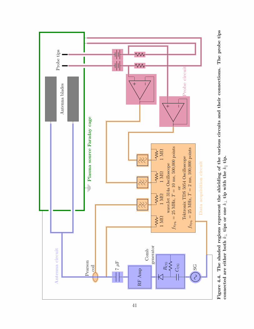
4.4 Experiment Electrical Circuit . . . . . . . . . . . . . . . . . . . . . . 41
4.5 Forward and Backward Branches of the Dispersion Relation . . . . . 45
5.1 Perpendicular Probes Autopower and Coherence Spectra in Argon . . 50
5.2 EIC Wave Perpendicular Wavenumber Measured in Argon . . . . . . 51
5.3 Perpendicular Probes Autopower and Coherence Spectra in Helium . 53
5.4 Parallel Probe Autopower and Coherence Spectra in Helium . . . . . 54
5.5 EIC Wave Real Wavenumbers Measured in Helium . . . . . . . . . . 55
B.1 Illustration of Cauchy’s Argument Principle . . . . . . . . . . . . . . 67
B.2 Types of Search Regions . . . . . . . . . . . . . . . . . . . . . . . . . 69
B.3 Root-Finding Recursion . . . . . . . . . . . . . . . . . . . . . . . . . 71
C.1 Plasma Parameter Panel . . . . . . . . . . . . . . . . . . . . . . . . . 75
C.2 Plasma Parameter Menu . . . . . . . . . . . . . . . . . . . . . . . . . 75
C.3 Solver Settings Panel . . . . . . . . . . . . . . . . . . . . . . . . . . . 77
C.4 Esipchuk-Tilinin Dispersion Relation Example . . . . . . . . . . . . . 81
D.1 Esipchuk-Tilinin Dispersion Relation Display . . . . . . . . . . . . . . 82
D.2 Data Import for Esipchuk-Tilinin Example . . . . . . . . . . . . . . . 83
D.3 Solver Settings for Esipchuk-Tilinin Example . . . . . . . . . . . . . . 84
D.4 Locations of Unstable Modes . . . . . . . . . . . . . . . . . . . . . . . 84
D.5 Example Dispersion Relation for Branch at x = 44 mm. . . . . . . . . 85
xiii

List of Symbols
⊥ Perpendicular to background magnetic field
‖ Parallel to background magnetic field
a Fourier image of quantity a
a∗ Complex conjugate of quantity a
a[n] Value of quantity a at nth step of an iteration
a Initial guess for value of a
B Magnetic field, G
cS Ion sound speed, m/s
D Dispersion relation
d Distance, m
E Electric field, V/m
fc,i Ion cyclotron frequency, cycles/s
fcut Cutoff frequency, cycles/s
fi Ion velocity distribution function
fi0 Background ion velocity distribution function
fi1 First-order perturbed ion velocity distribution function
fp,i Ion plasma frequency, cycles/s
fRF RF frequency, cycles/s
FW Windowed discrete Fourier transform
I Current, A
I Integral for Cauchy’s Argument Principle
I Fluorescence intensity
I0 Background fluorescence intensity
IIP In-phase fluorescence intensity
IQ Out-of-phase fluorescence intensity
In nth order modified Bessel function of the first kind
xiv

Jex Axial electron current density
Jm mth order Bessel function of the first kind
k Wavenumber vector, rad/m
kr Real component of the wavenumber, rad/m
ki Imaginary component of the wavenumber, rad/m
mi Ion mass, kg
ne Electron number density, /m3
ni Ion number density, /m3
p Plasma parameter
P Pressure, Pa
Po Neutral pressure, torr
P11, P22 Autopower spectrum, V2
P12 Crosspower spectrum, V2
R Region of the complex plane
Te Electron temperature, eV
Ti Ion temperature, eV
uB Magnetic drift velocity, m/s
ude E×B electron drift velocity, m/s
V Voltage, V
vA Alfven velocity, m/s
vd,i Ion drift velocity, m/s
vg Group velocity, m/s
vi Ion velocity, m/s
vph Phase velocity, m/s
vth,e Electron thermal velocity, m/s
vth,i Ion thermal velocity, m/s
Z Plasma dispersion function of Fried and Conte
xv

γ Coherence, rad/s
∆φ Phase difference, rad
θ Angle of propagation in xy-plane, rad
λD,e Electron Debye length, m
ν0 Atomic electron transition frequency, Hz
νDS Doppler shifted frequency, Hz
νL Laser frequency, Hz
ρe Electron Larmor radius, m
ρi Ion Larmor radius, m
τ Mean time between collisions, s
Φ Electric scalar potential, V
ω Angular frequency, rad/s
ωc,e Electron cyclotron frequency, rad/s
ωc,i Ion cyclotron frequency, rad/s
ωi Imaginary component of the angular frequency, rad/s
ωp,e Electron plasma frequency, rad/s
ωp,i Ion plasma frequency, rad/s
ωr Real component of the angular frequency, rad/s
xvi

Chapter 1
Introduction
1.1 Overview and Motivation
A plasma can sustain numerous plasma wave modes which span orders of magnitude
of frequency and wavelength. Unlike in regular fluids, long-range electromagnetic
interactions are as important as or even dominant over hydrodynamic interactions
in plasma systems, leading to markedly different behaviors. The disparity between
ion and electron masses, the anisotropy induced by background magnetic fields, and
particle kinetic effects are some of the characteristics particular to plasmas that allow
for more complex wave phenomena. This usually means that plasmas are dispersive
media in which the phase velocity of waves is a function of wave frequency. Plasma
wave modes are present in naturally occuring systems, such as electromagnetic ion-
cyclotron waves in Earth’s outer magnetosphere [1], and play roles in physical pro-
cesses like the acceleration of ions in Earth’s ionosphere [2] or the reconnection of
magnetic field lines in the solar corona [3]. On Earth, multiple engineering systems
use plasma waves for a variety of purposes: to sustain plasma discharges (e.g. by
depositing energy through helicon waves [4, 5, 6]), to heat plasmas (e.g. by selectively
coupling to tail electrons with lower-hybrid waves [7, 8]), or to measure plasma proper-
1

Figure 1.1. Hall effect thruster operating with xenon. Picture courtesy ofjpl.nasa.gov.
ties (e.g. by conducting reflectometry of high-frequency electron Langmuir waves [9]).
Additionally, unstable plasma wave modes (i.e. instabilities) affect both the theoreti-
cal understanding and operation of plasma devices (e.g. instability-induced turbulence
in tokamaks [10]).
In the field of electric propulsion, research concerning plasma waves and instabil-
ities is important as these phenomena impact the modeling, design, and certification
of plasma thrusters. In particular, the Hall effect thruster (HET), pictured in Fig. 1.1,
has been a focus of plasma wave research over the past decades as this device exhibits
oscillations in the 1 kHz – 60 MHz frequency range [11] which affect our fundamen-
tal understanding of the plasma physics of the discharge. As shown in Fig. 1.2, the
Hall effect thruster has an annular channel inside which propellant is ionized and
accelerated to generate thrust [12]. The crossed electric and magnetic field (E ×B)
configuration magnetizes electrons emitted by the cathode and causes them to pri-
2

Fig
ure
1.2
.S
chem
ati
csl
ice
of
Hall
eff
ect
thru
ster
3

marily drift in the azimuthal direction. Due to their larger mass, the ions are not
magnetized and instead are accelerated axially by the electric field, creating an ion
plume that is neutralized by a portion of the electrons emitted by the cathode.
While electron motion is mostly confined to the azimuthal E×B direction, there
is axial transport across the background magnetic field in order to close the electrical
circuit between cathode and anode. The axial electron current density can be written
as [13]
Jex = ene
(ExBz
)1
ωc,eτ, (1.1)
where ne is the electron number density, Ex is the axial electric field, Br is the radial
magnetic field, ωc,e = eBr/me is the electron cyclotron frequency, and τ is the mean
time between electron and neutral collisions (the most relevant type of collision for
classical cross-field transport). The inverse Hall parameter 1/ωc,eτ , which is directly
proportional to the cross-field electron mobility and axial electron current density, can
be calculated using measurements of Jex, ne, Ex, and Bz. However, as exemplified by
Fig. 1.3, the measured inverse Hall parameter exceeds the values expected by classical
transport models [14, 13], most notably in the region near the channel exit.
Explaining this non-classical or anomalous cross-field electron diffusion [14] which
causes the higher-than-expected Jex and associated electron mobility remains part
of ongoing research [15, 16, 17, 18, 19]. So far, numerical simulations of HETs have
relied on ad-hoc models of the anomalous transport with free parameters that are
adjusted until the simulation matches experimental data [18, 19]. From a theoretical
standpoint, it is suspected that plasma oscillations play an important role in the
plasma dynamics of the discharge [20, 21, 17], resulting in microturbulence or large-
scale structures [22, 23, 24]. Recent work has focused how the electron cyclotron drift
instablity could produce enhanced transport in these devices [25, 26, 27, 18]. However,
4

(a) Experimental measurements and classical theory predictions for theinverse Hall parameter, along with Bohm’s constant value of 1/16.
(b) Experimental and classical theory predictions for the inverse Hallparameter, along with Ref. [13]’s improved but still incomplete model.
Figure 1.3. Plots of anomalous transport as represented by the inverse Hallparameter 1/ωc,eτ , which is proportional to electron mobility. Reproduced fromRef. [13].
5

Hall effect thrusters are capable of sustaining many different types of oscillations [11]
and the results arising from including different wavemodes currently do not allow for
“definitive conclusions about the exact physical mechanism responsible for anomolous
transport” [18] to be drawn.
Though modeling and understanding (either theoretically or numerically) the ef-
fect of plasma waves and instabilities on plasma transport is a challenging task [28,
29, 19], initial steps can be taken by first characterizing the propagation and growth of
plasma wavemodes of interest. Quasilinear theory, for example, “include[s] the effects
of turbulence self-consistently through anomolous transport terms which depend on
the unstable mode or modes and which evolve in time and space as the macroscopic
plasma parameters evolve” [30]. This methodology yields turbulence-related terms for
particle fluid equations which depend on an instability’s propagation (which relates
to the wave’s frequency and wavelength) and linear growth rate (see, for example,
Eqs. 11–13 in Ref. [30]). This vital information is contained in the wavemode’s disper-
sion relation, which we discuss in the following section. Deriving explicit expressions
for quantities such as linear growth rate from a dispersion relation is unfortunately
not always analytically possible without enforcing assumptions that do not reflect
the plasma discharges encountered in real propulsion systems (e.g. ignoring plasma
parameter gradients or particle kinetic effects). Numerical characterizations of the
plasma dispersion relations are therefore necessary to provide the input for advanced
transport models like this. Similarly, measuring the plasma wavemodes’ dispersion
relation provides the needed verification for the models developed.
6

1.2 The Dispersion Relation
The fundamental concept employed to mathematically describe plasma oscillations
(or oscillations in any kind of media) is the dispersion relation, commonly written
as [31]
D(ω,k; p1, p2, . . .) = 0, (1.2)
where the function D relates the wave frequency ω and the wavenumber vector k to
plasma parameters pi such as electron temperature Te or background magnetic field
B0. The roots ω(k; p1, p2, . . .) or k(ω; p1, p2, . . .) of the above function (sometimes
referred to as branches) represent the allowed wavemodes that may arise in the plasma
system which D models. These roots can be complex, so they are typically written as
ω = ωr + iωi or k = kr + iki to distinguish the portion describing propagation (ωr or
kr) from that describing growth or decay (ωi or ki ). This interpretation corresponds
to expressing a physical quantity that oscillates in space or time due to a wave’s
presence (such as electron density ne or electric field E) as
a(x, t) = a0(x, t) + a1 exp(ik · x− iωt), (1.3)
where a0(x, t) is the background value of a(x, t) and a1 is the amplitude of the linear
perturbation induced by the wave.
The exact form of D depends on the model chosen to describe the plasma sys-
tem. For example, using the convention in Eq. 1.3 for ion density ni, ion velocity vi,
pressure P, and magnetic field B, we can linearize and combine the ideal magneto-
7

hydrodynamic (MHD) equations
∂ni
∂t+∇ · (nivi) = 0, (1.4)
nimi
(∂
∂t+ vi · ∇
)vi =
(B · ∇)B
4π− ∇(B ·B)
8π−∇P, (1.5)
∂B
∂t= ∇× (vi ×B), (1.6)(
∂
∂t+ vi · ∇
)(P
nγi
)= 0, (1.7)
to write the dispersion relation for electromagnetic Alfven wave modes [32, 33]
(ω2 − v2Ak
2‖)[ω4 − (v2
A + c2S)k2ω2 + v2
Ac2Sk
2‖k
2]
= 0, (1.8)
where vA = B0/õ0nimi is the Alfven velocity, cS =
√Te/mi is the ion sound speed,
and k‖ and k⊥ (with k2 = k2‖ + k2
⊥) refer to the components of k in the directions
parallel and perpendicular to the background magnetic field, respectively. Closed-
form analytical expressions are readily obtainable for the various branches of this
dispersion relation.
However, not all dispersion relations can be analytically solved like Eq. 1.8 for
ω(k) or k(ω). Such is the case for the general electrostatic dispersion relation for a
warm magnetized plasma [31]
k2⊥ + k2
‖ +∑
s
1
λ2D,s
×[1 +
n=∞∑n=−∞
(ω − k‖vd,s − nωc,s)Ts⊥ + nωc,sTs‖√2k‖Ts⊥
e−bIn(b)Z(ζn,s)
]= 0,
(1.9)
where In is the nth order modified Bessel function of the first kind, Z the plasma
dispersion function of Fried and Conte,
ζn,s =ω − nωc,s − k‖vd,s√
2 k‖vth,s, bs =
k2⊥v
2th,s
ω2c,s
, (1.10)
8

λD,s =√
ε0Ts/e2ns the species Debye length, vth,s =√
Ts/ns the species thermal veloc-
ity, vd,s the species drift velocity, and ωc,s = eB/ms the species cyclotron frequency.
Even simplifying this expression for limiting cases like isothermal species (Ts‖ = Ts⊥)
or fully magnetized electrons (be 1) does not produce analytically tractable re-
sults. Numerical techniques are therefore used to successfully solve for the roots of
complicated dispersion relations like this.
However, even if analytically or numerically solvable, the models used to derive
a particular dispersion relation may integrate assumptions which do not reflect the
true nature of the plasma studied. For example, models which assume a homogeneous
plasma do not capture the effects spatial gradients of plasma parameters, like those
of density [34] or magnetic field [11] in Hall effect thrusters, have on the propagation
or stability of wavemodes. Similarly, simpler but more analytically-tractable fluid
models can fail to capture modes of propagation which rely on the inclusion of kinetic
effects, such as with the neutralized ion Bernstein wave [35, 36]. Experimental mea-
surements of the dispersion relation ultimately provide the necessary verification for
the theoretical framework established to understand the plasma wave physics. This
can be a challenging undertaking as experimental diagnostics can perturb the state
of the plasma, particularly when physical access to the locations is not easy in real
plasma systems and devices. Additionally, the advanced equipment sometimes nec-
essary to perform these measurements can present a high financial barrier and have
limited compatibility with different gases.
1.3 Thesis Objective and Structure
Motivated by the importance to experimentally characterize plasma wavemodes in en-
gineering devices like plasma thrusters or natural settings like Earth’s ionosphere to
better understand the underlying physics, this dissertation presents the Active Wave
9

Packet Injection (AWPI) diagnostic, an experimental diagnostic used to measure
dispersion relations in low-temperature laboratory plasmas using harmonically-rich
wave packets. We manufacture a prototype of the diagnostic and integrate it into an
existing experimental testbed to validate its perfomance. We also complement this
experimental investigation with numerical characterizations of relevant plasma wave-
modes using the Plasma Rocket Instability Characterizer (PRINCE), a numerical
software which solves for the roots of arbitrary dispersion relations over a versatile
and customizable parameter space.
We begin in Chapter 2 with a review of existing techniques for measuring plasma
dispersion relations along with a discussion of the procedure for numerically solving
for the roots of dispersion relations. Chapter 3 details the relevant signal analysis
methodologies and hardware implementation of the AWPI diagnostic, which result
in the successful generation of harmonically-rich wave packets in the 1-1000 kHz fre-
quency range. We describe in Chapter 4 the low-temperature magnetized RF plasma
source in which we implement the AWPI diagnostic to measure the dispersion rela-
tion of electrostatic ion-cyclotron (EIC) waves. We discuss our results in Chapter 5,
followed by concluding remarks in Chapter 6. a a∗ a[n] a
10

Chapter 2
Review of Existing Techniques
In this chapter we overview existing experimental techniques for measuring disper-
sion relations. We first discuss the difference between passive and active probing
of a plasma. We then briefly describe the physics behind three common techniques:
plasma-immersed probe interferometry, laser-induced fluorescence, and collective light
scattering. We note both strengths and weaknesses of each technique to contextualize
and motivate the development of the AWPI diagnostic. We also include a discussion
of typical procedures to numerically solve for the roots of dispersion relations and the
difficulties that arise due to the nonlinear nature of the complex functions commonly
encountered in plasma physics. This is an important task to overview as it enables the
direct comparison of theory to measurements and provides some of the background
for the PRINCE software described in the appendices.
2.1 Measuring Plasma Dispersion Relations
Various techniques exist to experimentally characterize the spatial and temporal spec-
tra of different plasms parameters. Depending on the plasma system studied, nat-
urally excited plasma waves can produce sufficiently strong signals for passive diag-
nostics to detect or ‘listen’ to. Sometimes, though, the plasma modes of interest
11

may not be naturally excited or, if they are, do not produce signals that rise above
background measurement noise, resulting in low signal-to-noise ratio (SNR) measure-
ments which require additional processing to extract meaningful information [37, 20].
In these cases, antennae of various geometries are implemented alongside the passive
diagnostics to actively inject waves into the plasma [38, 36, 39, 40] (a procedure not
unique to plasma wave investigations, but also for objectives such as discharge cre-
ation [41, 42, 6] or plasma heating [8, 43]). This active injection of waves ‘rings’ the
plasma to capture both the phase and growth components of the linear dispsersion
relation, which can be obscured once naturally excited modes reach the saturation
stage. Past active injection experiments have generally been limited to single- or
dual-frequency wave launching [44, 36, 40, 45], so the dispersion relation is measured
one frequency at a time. In the following sections we briefly review three techniques
which measure dispersion relations of naturally excited or actively injected plasma
waves.
2.1.1 Plasma-Immersed Probe Interferometry
Probe interferometry relies on the cross-correlation of the time-dependent voltage or
current traces of two or more probes physically immersed in a plasma at known loca-
tions [46, 37]. Using a single probe or probes outside the plasma usually only provides
information on the frequency spectrum of the oscillations; measuring the dispersion
relation requires insight into the spatial structure of the waves. The probes imple-
mented measure a physical quantity which the plasma wave causes to vary in time,
such as ion-saturation-current probes to measure ni [36, 40, 47, 20] or magnetic in-
duction probes (also called B-dot probes) to measure B [48, 49]. At a given frequency
ω, the real part of the wavenumber in the direction parallel to the line between the
12

p(x, t)
∆φ
d12
Figure 2.1. Two probes immersed in the plasma take time traces of the valueof the oscillating plasma parameter p(x, t) at two known spatial locations.
two probe tips is
kr =∆φ
d12
, (2.1)
where ∆φ is the phase difference between the two probe signals and d12 is the distance
between the probes. The relative signal between the probe signals also provides
information on the growth or decay of the wave mode (i.e. ki). Though simple to
implement, the probes may alter the state of the plasma by locally cooling both
neutral and charged species in high-density discharges, leading to lower temperatures
or higher densities [50]. Even in low-density discharges, plasma sheath effects and
the electrical biasing of the probes (in the case of particle flux probes) require careful
consideration to correctly determine bulk plasma properties [9]. The physical scale of
the probes and the possibility of sheath overlap set limits on the smallest resolvable
spatial scales, which usually lie in the millimeter range (k less than ∼ 650 /m) [51, 27].
A more detailed discussion of the signal analysis involved in this technique is presented
in Section 3.1 as it serves as the basis for our AWPI diagnostic.
13

2.1.2 Laser-Induced Fluorescence
The non-intrusive laser-induced fluorescence (LIF) technique measures the back-
ground (fi0) and first-order perturbed (fi1) ion velocity distribution functions (IVDFs)
by exploiting forced and spontaneous atomic electron transitions in the ion popula-
tion [9, 52, 53]. A laser excites bound electrons to a metastable state in order to
measure the intensity of the induced fluorescence from the subsequent spontaneous
relaxation. If the perturbation fi1 is due to a traveling plasma wave, measuring the
background (I0), in-phase (IIP ) w.r.t. the plasma wave’s phase, and out-of-phase
or quadrature (IQ) components of this fluorescence as a function of laser frequency
provides a way to determine the plasma wave’s dispersion relation. This technique
has been used, for example, to measure the parallel and perpendicular wavenum-
bers of electrostatic ion-cyclotron waves in linear magnetized RF plasma sources [54]
or as part of investigations concerning plasma heating through beating electrostatic
waves [55, 56].
Ener
gy(1
03cm−
1)
Ener
gy(e
V)
135 16.7
140 17.4
145 18.0
150 18.6
155 19.2
160 19.8
4P 4P 0 4D 4D0 4F
668.61 nm
1→ 2442.72 nm
2→ 3
Figure 2.2. In this example Ar II scheme, the laser induces the atomic electrontransition 1→ 2 (red). The fluorescence emitted by the relaxation 2→ 3 (purple)is measured. Diagram developed based on Refs. [57, 58, 53].
14

The atomic electron transitions for the forced excitation and spontaneous re-
laxation used in gas-specific LIF schemes involve easily distinguishable light wave-
lengths so that the input laser light does not interfere with the fluorescence measure-
ment [52, 59, 53, 60, 61, 62]. Fig. 2.2 depicts one such example scheme for singly-
charged argon ions which works with radiation in the visible spectrum. Laser light
whose frequency νL matches the atomic electron transition frequency ν0 (in this case
corresponding to a wavelength of 668.61 nm) excites electrons from the stable 3d4F7/2
state (1) to the metastable 4p4D05/2 state (2). The excited electrons spontaneously
relax from this metastable state to the stable 4s4P3/2 state (3) by emitting fluorescent
radiation at a frequency different than ν0 (in this case corresponding to a wavelength
of 442.72 nm). However, since the ion population has a non-zero temperature that
gives the ion velocity distribution function a finite width, only a fraction of the ion
population undergoes this process. Ions with velocity vi parallel to the the laser beam
encounter a Doppler shifted laser frequency
νDS = νL
(1 +
vi
c
), (2.2)
so only those with vi = 0 experience the transition 1→ 2 when the laser is tuned to
ν0. Ions with non-zero vi along the laser scanning axis require νL = νDS for excitation,
which in the non-relativistic limit |vi/c| 1 yields the relation
vi =c
ν0
(νL − ν0) (2.3)
between ion velocity and laser frequency. Sweeping νL about ν0 excites different
portions of the ion population, allowing the optically-measured fluorescent intensities
mentioned above to be correlated with ion velocities. Solutions to the ion Vlasov
equation perturbed with either an electrostatic wave’s potential E1 = −ikΦ1 exp(ik ·
x− iωt) or an electromagnetic wave’s fields E1 and B1 such that k×E1 = ωB1 [63]
15

are fit to the fluorescent intensity measurements to calculate the wave ω and k. The
full data-reduction procedure for the case of an electrostatic wave is described in
Appendix A (see Refs. [54, 55, 63] as well); the case of an electromagnetic wave is
covered in Ref. [63].
While attractive for its non-intrusive nature, the LIF technique takes measure-
ments at a single spatial location in the plasma and uses the dispersion relation from
Eq. 1.9 or its electromagnetic equivalent to provide closure for the fitting procedure
of the data [54, 63]. These dispersion relations do not include the effects of plasma
parameter gradients, which may be relevant in real plasma devices [64, 11, 65]. Addi-
tionally, the diagnostic involves costly equipment and two optical lines-of-sight access
points to the plasma volume, making it challenging to implement. Its reliance on
fluorescence makes it incompatible with certain gases (e.g. He II) and can limit a
particular laser system’s applicability to multiple gases.
2.1.3 Collective Light Scattering
Another non-intrusive technique, collective light scattering scatters laser light off
oscillating plasma electrons to measure the frequency spectrum of electron plasma
waves with a wavenumber vector defined by the scattering geometry [66]. In addition
to dispersion relation measurements, this diagnostic can provide information on the
form factor, amplitude, and spatial distribution of electron density fluctuations [67].
This diagnostic has been used in particular to investigate the E × B electron drift
instability in Hall effect thrusters [67, 68, 25].
Free electrons undergoing oscillatory motion in the plasma scatter incident laser
light with wavenumber vector kinc. The scattered light has a wavenumber vector
ksc which, as shown in Fig. 2.3, is at an angle α with respect to kinc. The sig-
nal of this scattered light depends on α and the associated analyzing wavenumber
k = ksc − kinc; measuring this scatterred light provides information on the spatial
16

ksc
kinc
k
α
Figure 2.3. Scattering by electrons of incident light with wavenumber vectorkinc produces light with wavenumber vector ksc. Measurements of the spatialFourier transform of electron density at different k = ksc − kinc are taken byvarying the angle α or by rotating the scattering plane. Based on Ref. [67].
Fourier transform of the electron density at that k [67, 68]. Varying α or rotating
the scattering plane as a whole allows for measurements at different values of k.
Recording the time-dependent scattered light signal using a superheterodyne optical
interference technique provides information on the temporal Fourier transform of the
electron density, yielding a measurement of the wave frequency ω as a function of the
geometry-defined k.
The full mathematical details of the collective light scattering diagnostic are pre-
sented in Ref. [67]. Similar to the LIF technique, collective light scattering requires
costly equipment and optical access to the plasma volume, also making its implemen-
tation challenging. Alignment and equipment constraints have only allowed for prob-
ing wavenumbers greater than ∼ 4000 /m at frequencies in the MHz range [67, 68, 25],
so the ability of this technique to measure low-frequency or long-wavelength wave-
modes is not certain. Moreover, since the scattering is due to fluctuations in the
electron density, only compressible electrostatic wavemodes can be detected with this
method.
17

2.2 Numerically Characterizing Plasma Disper-
sion Relations
Measurements taken by the above techniques are commonly compared to numerical
solutions ω(k) or k(ω) which satisfy Eq. 1.2 to validate theoretical plasma models.
This entails finding the complex roots of an analytic (or meromorphic at worst) func-
tion over a multidimensional complex space. This task is commonly faced across
multiple disciplines, ranging from pure or applied mathematics [69, 70, 71, 72] to var-
ious engineering fields [73, 74, 75]. Since a dispersion relation fundamentally describes
oscillatory motion in a medium, numerically finding its roots in different configura-
tions of varying media has been widely researched [76, 77, 78, 79, 80]. Given that
dispersion relations many times are nonlinear functions, one strategy to simplify the
problem is to construct a complex polynomial which has the same roots as the non-
linear function and pass this to a variety of efficient polynomial-root solvers [69, 70].
Alternatively, if this is not an adequate or viable simplification to perform, a com-
mon tactic is to use root-finding algorithms that can handle nonlinear functions, such
as Newton-Raphson’s method or the secant method [81, 82]. Typically, methods
like these require the input of one or more values near the root (i.e. initial guesses)
to initiate an iterative procedure which eventually convergences to the ‘true’ value
(i.e. within numerical tolerance) of the root. While these methods generalize to
higher dimensions [82], it is nevertheless common to reduce the dimensionality of the
input variable space when searching for the roots of dispersion relations in plasma
physics. For example, k components are rewritten as functions of just one k com-
ponent (e.g. ky = ky(kx) and kz = kz(kx)), removed by considering limiting cases
(e.g. k⊥ → 0 for purely parallel propagation), or, if possible, grouped into nondi-
mensional variables (e.g. k⊥/k‖) [83, 84, 35, 31, 11, 40, 34]. Usually two independent
variables remain, one of which is iterated over N steps (e.g. kx ∈[k
[0]x , k
[1]x , . . . , k
[N−1]x
])
18

Stop
Yes
Is n > N?
Solve for ω[n] using Newton-Raphson
Initialize n = 0,D[0](ω, k[0]‖ ), and ω[0]
Simplify to D(ω, k‖) by evaluating k⊥ = k⊥(k‖)
Simplify to D(ω,k) by evaluating the pi
Select D(ω,k; pi)
Start
Non+ = 1
Update D[n](ω, k[n]‖ )
and ω[n] = ω[n−1]
Figure 2.4. An example procedure for numerically characterizing a branch ω(k‖)of the function D(ω,k; pi). There are N discrete values of k‖ for which we wantto find an ω using an initial guess ω such that Eq. 1.2 is satisfied.
and the other which is the root sought (e.g. ω such that D[n](ω, k[n]x ) = 0), where the
superscript [n] denotes evaluation at the n-th step of the iteration. Fig. 2.4 depicts
the steps for an example procedure where the goal is to compute ω(k‖).
As intricate as finding the complex root of a single-variable nonlinear function
already is (a task “equivalent to finding the vector roots of a system of two nonlinear
equations” [85]), a further difficulty arises if multiple roots of the dispersion relation
are present in the region of (ω,k)-space studied, which is not uncommon for dispersion
relations in plasma physics [35, 31]. Determining the number and potential location
19

of these roots a priori is not trivial, complicating the choice of adequate initial values
to input into root-finding algorithms. Additionally, even if the number of roots is
somehow known, which root an iterative root-finding algorithm converges to can be
a highly sensitive or even chaotic function of the input values, giving the algorithms
poor global convergence properties [82]. As Fig. 2.5 illustrates, even functions as
simple as complex polynomials exhibit undesired behavior if we feed a poor initial
guess to an algorithm like Newton-Raphson. This means that resolving the desired
branch of a dispersion relation could involve time-consuming sweeps over the input
parameter space. Previous work has tried to address this complication by plotting
the contours Re (D(ω,k)) = 0 and Im (D(ω,k)) = 0 over a region in (ω,k)-space to
identify where they intersect and thereby provide the initial guess for the root [81, 85].
A similar graphical strategy uses the argument of D(ω,k) to generate a slope field
plot in the complex plane and locate ‘vortices’ which encircle the roots [86, 87]. Both
of these methods require (1) active human input, which can become inconvenient for
investigations over larger spans of the pi and (ω,k)-space, and (2) repeated evaluation
of D at unneeded locations in the complex plane, which becomes computationally
costly for more advanced dispersion relations.
Instead, it is desirable to develop an automated procedure to numerically char-
acterize the roots of arbitrary dispersion relations. Provided a specific dispersion
relation D(ω,k; pi) along with a set of pi and the search region in (ω,k)-space, two
goals should be accomplished autonomously:
1. Global root-finding: Determine the number and initial location of all roots in
the relevant search region.
2. Local root-tracking: Track the location of each root as the specified iteration
variable varies.
20

Figure 2.5. Newton fractal generated by searching for the roots of the poly-nomial z5 − 1 using the Newton-Raphson method. The five different colorscorrespond to the five different roots the iteration converges to given the initialguess. The black dots depict the location of the five roots.
21

The nonlinear nature of dispersion relations in plasma physics especially complicates
the first of these goals. Successfully accomplishing it mitigates several issues that
can arise when carrying out the second goal; the numerical algorithms and PRINCE
software described in Appendices B and C, respectively, are designed to have better
global convergence propoerties than previous techniques in order to achieve this.
2.3 Chapter Summary
The experimental techniques reviewed in this chapter showcase the trade-off between
the simplicity (both in terms of analysis and hardware implementation) and the intru-
siveness of diagnostics for measuring plasma dispersion relations. The AWPI diagnos-
tic we develop in Chapter 3 opts for simplicity but integrates waveform shaping into
the signal design to provide more expedited measurement capabilities than previous
intrusive diagnostics. We also overviewed several existing techniques for numerically
solving for the roots of dispersion relations to provide background for the PRINCE
software which we use to provide complementary numerical characterizations of the
wavemodes we measure using the AWPI diagnostic.
22

Chapter 3
Active Wave Packet Injection
Diagnostic1
In this chapter we describe the Active Wave Packet Injection (AWPI) diagnostic, an
active diagnostic which emits harmonically-rich wave packets in a plasma in order to
measure dispersion relations. We overview the frequency-space interferometric signal
analysis for calculating wavenumbers as a function of wave frequency. We describe
the manufacture of an AWPI diagnostic for use in a low-temperature plasma source,
which involves the design of a harmonic comb generating circuit, an antenna, and
receiver ion-saturation-current probes. The diagnostic produces dozens of harmonics
of an input square wave’s fundamental frequency in the 1-1000 kHz range.
3.1 Overview of Methodology
Active wave injection systems for measuring plasma dispersion relations have con-
sisted of an emitter probe or antenna along with two or more receiver ion-saturation-
1This chapter is based on work being prepared to be submitted for publication and previouslypresented in [88]: Rojas Mata, S. and Choueiri, E.Y., ”Plasma Dispersion Relation Measurementsthrough Active Injection of Wave Packets,” 36th International Electric Propulsion Conference, Vi-enna, 2019.
23

k(ω)
Compression Rarefaction
Vin(t)
I2(t)I1(t)Emitter probe or antenna Ion-saturation-current probes
Figure 3.1. The antenna excites traveling compressions and rarefactions ofplasma density which result in time-dependent ion-saturation-current tracesrecorded by the receiver probes downstream.
current probes [89, 36, 86, 40]. In Fig. 3.1 we show an example system with an
antenna and two receiver probes immersed in the plasma. The system can be gener-
alized to contain more receiver probes, so that each pair of receiver probes measures
the wavenumber along the direction parallel to the line joining their tips. Addition-
ally, as mentioned in Section 2.1.1, other kinds of probes such as B-dot probes can
be used as needed to measure the relevant plasma parameter. For the case of elec-
trostatic waves, a time-dependent voltage signal Vant(t) sent to the antenna excites
the wave and causes traveling compressions and rarefactions of plasma density to
pass by the receiver probes located downstream. Control over the harmonic con-
tent of Vant(t) allows targeting of the expected frequency range (e.g. from theory or
numerical simulation) of the plasma wave mode in question.
Analysis of the current traces I1(t) and I2(t) provides information about the
wavenumber k as a function of the wave frequency ω. Though previous work used
sinusoidal excitations and our AWPI diagnostic uses harmonically-rich excitations,
the frequency-domain analysis to measure the dispersion relation we use is applicable
to both. To identify coherent wave propagation over background random noise in
the signals recorded, we compute spectrum and correlation estimates of the digitally
24

recorded I1(tn) and I2(tn). We follow a nonparametric signal processing procedure
similar to Welch’s method for estimating power spectral densities [90] to produce
estimates of auto- and crosspower spectra as well as an estimate of the coherence
spectrum between two probe signals [46, 91, 92].
3.1.1 Estimation of Power and Coherence Spectra
Assume the data sets of the recorded current traces I1(tn) and I2(tn) are of length N
points. Since we want a measure of the variance in the power spectra (i.e. provide
error bars for the measurements), we do not calculate spectra of the entire N -long
data set. Instead, we divide each set into S equal subsets of length M points to
produce the sets I1,1, I1,2, . . . , I1,j and I2,1, I2,2, . . . , I2,j, j ∈ [1, S]. Using several
shorter data sets allows us to calculate the signals’ variance and decrease the effect of
random noise, but comes at the cost of increased frequency increments ∆f = fn−fn−1
in the spectra (and thus increased spectral ‘leakage’) [92, 91]. To partially mitigate
this, we overlap successive data segments by 50% as pictured in Fig. 3.2 so that we can
construct longer subsets than if there was no overlap. Such overlap of data subsets is
the distinguishing factor of Welch’s method [90], while the specific amount of overlap
is a common recommendation in the signal processing literature [91, 92].
We then take the windowed discrete Fourier transform
I1,j(fn) = FWI1,j(tn) and I2,j(fn) = FWI2,j(tn) (3.1)
of each data subset. We use a Hanning window “since it provides a good compro-
mise between amplitude accuracy and frequency resolution” [92]. We calculate the
autopower spectra P11, P22 of the current traces I1 and I2 by averaging over the au-
25

I1(tn)
tn
I1,1(tn)
I1,2(tn)
I1,3(tn)
I1,4(tn)
· · · M
Figure 3.2. For each current trace we generate overlapping data subsets oflength M whose extent is illustrated above by the red and green bars. Usingmore subsets gives better error estimates but a larger frequency increment forthe spectra.
topower spectra of the data subsets, so that
P11(fn) =A
S
S∑j=1
I∗1,j(fn)I1,j(fn) and P22(fn) =A
S
S∑j=1
I∗2,j(fn)I2,j(fn), (3.2)
where
A =1
M2P 2W
with PW = |FW1| (3.3)
is an amplitude correction factor to account for the power of the window PW . Simi-
larly, we compute the crosspower spectrum
P12(fn) =A
S
S∑j=1
I∗1,j(fn) I2,j(fn) (3.4)
26

and a normalized version of it called the coherence spectrum
γ12(fn) =P12(fn)[
P11(fn)P22(fn)]1/2 , (3.5)
both of which provide information about correlated signals present in the probes.
Specifically, the magnitude of the coherence spectrum measures how linearly related
the two probe signals are, with |γ12| = 0 denoting no relation and |γ12| = 1 denoting a
complete linear relation. We consider wave propagation to be coherent when |γ12| >
0.95 and its error is less than 0.05. Note that, if instead of using estimates of the
spectra in Eq. 3.5 we used the actual spectra of the N -long data sets, then |γ12| =
1∀ fn and we could not identify coherent wave propagation over random noise.
3.1.2 Dispersion Relation Measurement
The real wavenumber spectrum of coherently propagating waves is
kr(fn) =ArgP12(fn)
d12
, (3.6)
where d12 is the distance between the two receiver probes. The imaginary wavenumber
spectrum, which represents spatial growth or decay, is given by
ki(fn) = − 1
2d12
log
[P22(fn)
P11(fn)
]. (3.7)
We can also calculate the phase and group velocities
vph =ω
krand vg =
dω
dkr. (3.8)
27

3.2 Harmonic Comb Generating Circuit
For sinusoidal excitations in a plasma, γ12 = 1 just for one value of fn (the wave
driving frequency), so the data acquisition and analysis would have to be repeated
mutliple times for different driving frequencies to produce multiple measurements of
kr ad ki. We seek to expedite the process by sending harmonically-rich excitation
signals to the diagnostic’s antenna, which can be particularly advantageous in pulsed
plasma experiments [93, 86]. We therefore construct a circuit capable of producing
dozens of harmonics with comparable amplitudes of a fundamental frequency to excite
and record coherent wave packets (i.e. γ12 = 1 for multiple values of fn) instead of a
single coherent wave in the plasma.
We base the design of our harmonic comb generating circuit on previous work
that sought a size-, weight-, and power-constrained solution to in-situ diagnosing of
wireless devices [94]. As shown in Fig. 3.3a, the circuit contains a square wave signal
generator, a high-pass filter, and a diode, the latter two of which are depicted in
Fig. 3.3b. A square wave contains only odd-integer harmonics of its fundamental fre-
quency, which decrease in amplitude inversely proportional to harmonic number. The
high-pass filter acts as a differentiator and attenuates the lower-frequency harmonics
Square wavesignal generator
High-pass filter
Diode
(a) Schematic
High-pass filter
Diode
SGRF Amp
(b) Hardware
Figure 3.3. The high-pass filter and diode are passive but the oscillator is asignal generator capable of outputing square waveforms. Based on the designin Ref. [94].
28

of the square wave to decrease the disparity between amplitudes (i.e. it accentuates
the sharp edges of the square wave). The directional nature of the diode breaks the
positive-negative symmetry of the signal to generate the missing even-numbered har-
monics. We amplify this harmonically-rich signal with an E&I 1140LA broadband
power amplifier before sending it to the diagnostic’s antenna.
The expected frequency range of the plasma wavemode studied determines the
high-pass filter’s cutoff frequency fcut and the fundamental frequency for the square
wave. Since the experimental investigation described in Chapter 4 involves waves with
frequencies in the tens to hundreds of kilohertz, we build the four different high-pass
filters detailed in Table 3.1. We test the circuit’s ability to send harmonically-rich
signals to the diagnostic’s antenna by inputing square wave frequencies in the 4-
20 kHz range. We measure the antenna voltage Vant(tn) and antenna current Iant(tn)
to estimate these signals’ autopower spectra through the same procedure as that of the
probe signals in the previous section. We also calculate their linear spectra, which is
the square root of the autopower spectra and correspond to measurements of voltage
and current amplitudes at each frequency. Fig. 3.4 shows these four spectra for HPF
1 and an input 4 kHz square wave; Fig. 3.5 does the same but for HPF 4 and an input
10 kHz square wave. The comb structure of all the signals is clear, with hundreds
of harmonics present at similar power levels. This signal structure provides a means
to excite waves at multiple frequencies simultaneously and at similar power levels,
thereby creating the harmonic wave packet that will propagate through a plasma so
we can measure the dispersion relation in one shot.
Table 3.1. Component Values for High-Pass Filters
HPF 1 HPF 2 HPF 3 HPF 4Capacitance (C) 24.6 nF 9.8 nF 16.5 nF 7.8 nFResistance (R) 327 Ω 328 Ω 99.2 Ω 99.1 Ω
Cutoff Frequency (fcut) 20 kHz 50 kHz 100 kHz 200 kHz
29

Iant
Iant
Figure 3.4. These spectra correspond to a circuit with HPF 1 from Table 3.1and a 4 kHz square wave input. The signal at the fundamental frequency isused as the reference for the decibel normalization.
30

Iant
Iant
Figure 3.5. These spectra correspond to a circuit with HPF 4 from Table 3.1and a 10 kHz square wave input. The signal at the fundamental frequency isused as the reference for the decibel normalization.
31

3.3 Antenna and Probes Design and Manufacture
We build the antenna and probe system photographed in Fig. 3.6 and schematically
depicted in Fig. 3.7. Two 1.5 cm by 5 cm, 0.51 mm thick molybdenum plates resting
on alumina stand-offs which attach to a 1.27 cm diameter G-10 tube consitute the
antenna. We choose this antenna geometry as previous investigations used it to excite
electrostatic modes in magnetized plasmas [36, 40]. Tungsten wires attach each plate
to coaxial cables which connect the antenna back to the harmonic comb generating
circuit described above. The circuit does not have a tuner for matching impedance
between the antenna and the plasma load; tuners usually only achieve matching at one
or two frequencies [6, 45] and we wish to couple to the plasma at multiple frequencies
simultaneously. For our proof-of-concept investigation in the following chapters, we
instead decide to operate our plasma source (see Chapter 4) at conditions for which
we excite wave packets to validate the AWPI methodology. This tactic of matching
the plasma to the antenna has been successful in past experiments which also did not
have tuners in their antenna circuit [38, 36, 40].
The diagnostic has three receiver probes to measure wavenumbers in the directions
parallel and perpendicular to the plane of the antenna blades which, in the experi-
mental implementation discussed in Chapter 4, also correspond to k‖ and k⊥. The
perpendicular tips are 0.1 cm apart and the parallel tip is 0.5 cm away from these;
all sit ∼1 cm away from the antenna blades. As mentioned in Section 2.1.1, sheath
overlap concerns limit the physical size and separation of plasma immersed-probes.
However, even the distance between the perpendicular tips (0.1 cm) is much larger
than the electron Debye length (∼30 µm) in our plasma source, so we do not expect
sheath overlap. These probe tips are 2 mm long, 0.254 mm thick tungsten wires
housed inside alumina tubes cased in copper tubes for capacitive shielding and glass
tubes for protection from the plasma environment. We bias the tips to -27 V with
batteries to operate them as uncompensated ion-saturation-current probes. We use
32

Antenna blades
k‖ tip
k⊥ tipsReceiver probes
Figure 3.6. All wiring going to the antenna and probe tips runs through G-10 tubes to protect it against the plasma environment. Zirconia paste coatsinterfaces between wires and housing to prevent damage.
the ion saturation-current Isat as a proxy for the ion density ni which, for electrostatic
modes, is related to the wave potential Φ by [20]
Φ ≈ Te
e
ni1
ni0
≈ Te
e
Isat1
Isat0, (3.9)
where Te is the electron temperature and the 0 and 1 subscripts refer to the back-
ground and linear-perturbation values of the quantity, respectively (see Eq. 1.3).
Assuming isothermal plasma compressions, measuring the fluctuations of Isat at the
two probes then gives us insight into spatiotemporal characteristics of electrostatic
33

5cm
1.5cm
1.27
cm
Mb
W
Al 2O
3Al 2O
3
3cm
G-10
Coaxcable
0.51
mm
thick
Glass
Copper
Al 2O
3
Antenna
blade
k‖
k⊥
Probetips
B0
Top
view
Fig
ure
3.7
.T
he
bott
om
pro
be
arm
has
two
pro
be
tip
sth
at
measu
reth
ew
avenu
mb
er
inth
ed
irecti
on
perp
en
dic
ula
rto
the
pla
ne
of
the
ante
nn
ab
lad
es,
wh
ich
inou
rexp
eri
ment
corr
esp
on
ds
tok⊥
.T
he
up
per
pro
be
arm
has
on
lyon
ep
rob
eti
p,
wh
ich
incom
bin
ati
on
wit
hon
eof
the
oth
er
two
pro
bes
(see
inse
tto
pvie
w)
measu
res
the
wavenu
mb
er
inth
ed
irecti
on
para
llel
toth
eaxis
of
the
G-1
0tu
bes,
wh
ich
inou
rexp
eri
ment
corr
esp
on
ds
tok‖
.
34

wavemodes. The wavemodes we investigate in our plasma source are under 1 MHz
in frequency, which is well below the ion plasma frequency of 17 MHz for argon and
33 MHz for helium (see Tables 4.2 and 4.3). This ensures that the sheath can adjust
fast enough to the varying bulk plasma density and plasma potential [6] so that our
use of the ion saturation-current as a proxy for ni remains valid.
3.4 Chapter Summary
In this chapter we overviewed the signal analysis procedure to measure the disper-
sion relation of a plasma using the active injection of wave packets. We described
our design for the harmonic comb generating circuit, antenna, and probes which to-
gether constitute our AWPI diagnostic. We demonstrated the reliable generation of
harmonically-rich signals in the 1-1000 kHz range which we will use to measure the
dispersion relation of low-frequency ion waves in the experimental appartus described
in the following chapter.
35

Chapter 4
Plasma Source for Low-Frequency
Ion Wave Studies
In this chapter we provide a brief technical overview of the magnetized RF plasma
source in which we use the AWPI diagnostic to measure low-frequency electrostatic
wave modes. We provide several representative plasma parameters for the source.
Based on these, we present the theory behind the electrostatic ion waves accessible
for excitation when operating with argon or helium along with illustrative numerical
characterizations obtained using the PRINCE software.
4.1 RF Plasma Source
We use the plasma source pictured in Fig. 4.2 in which previous studies explored
ion heating through beating electrostatic waves [95, 55]. Fig. 4.1 depicts a cutaway
schematic of the experiment created using the detailed design schematic found in
Ref. [55]. The vacuum vessel is a 132 cm long, 15.5 cm inner diameter quartz tube (an
upgrade from the previous pyrex tube) which is housed inside a 122 cm long, 10 ring
solenoid. A water cooled 19.1 cm outer diameter, 22 cm long saddle antenna surrounds
the quartz tube at one end of the vessel. A 1.25 kW RF source which operates at
36

Mea
sure
men
tar
ea
Sol
enoi
dca
sing
OD
:50
.2cm
,L
:59
cm
Sad
dle
ante
nna
OD
:19
.1cm
Al
flan
geO
D:
18cm
Pyre
xw
indow
OD
:10
.16
cm
Mag
net
icco
ils
Quar
tztu
be
ID:
15.5
cmR
ail
tosu
pp
ort
tub
e
To
pum
p
Fig
ure
4.1
.T
he
are
aw
here
we
measu
reth
ed
isp
ers
ion
rela
tion
isat
the
oth
er
en
dof
the
qu
art
ztu
be
than
the
RF
sad
dle
ante
nn
ato
red
uce
the
back
gro
un
dn
ois
e.
Tw
op
ad
ded
G-1
0h
alf
rin
gs
(not
dep
icte
d)
wh
ich
roll
alo
ng
the
rail
ssu
pp
ort
the
qu
art
ztu
be.
37

Probe tips
Antennablades
Solenoid coils
Feedthroughs
Figure 4.2. The saddle antenna sustains the 13.56 MHz argon discharge insidethe quartz vessel. Feedthroughs in the aluminum cross provide physical accessto the plasma. The AWPI diagnostic sits near the center of the discharge.
13.56 MHz powers the saddle antenna while an L network with two Jenning 1000 pF
3 kV variable vacuum capacitors matches the RF signal to the plasma discharge with
a voltage standing wave ratio (VSWR) in the range 1 − 1.4. At the other end of
the vessel, an aluminum cross connects the quartz tube to a 140 l/s turbomolecular
pump which is backed with a Varian TriScroll 300 pump. A KJLC 300 series gauge
monitors the neutral pressure in the chamber; the ultimate pressure achievable is less
than 0.1 mTorr. The solenoid comprises two klystron Varian 1955A magnets placed
end to end, which generate an axial background magnetic field. Table 4.1 presents
the source’s typical operational parameters.
38

Table 4.1. Plasma Source Operational Parameters
Parameter Value Parameter ValueRF Power (PRF ) 250 W RF Frequency (fRF ) 13.56 MHz
Background Magnetic Field (B0) 526 G Neutral Pressure (Po) 0.1-5 mTorr
We operate the source with either argon or helium. Radial profiles for the electron
temperature and electron density when operating with argon reported in Ref. [55] are
reproduced in Fig. 4.3. Along with these, we also use ion temperature and background
magnetic field values reported in the same reference to construct Table 4.2 to present
representative values of various plasma parameters. These reflect the plasma state in
the near-centerline region r ≈ 0− 1.5 cm where we measure dispersion relations with
the AWPI diagnostic. We do not have corresponding measurements for these plasma
parameters when operating with helium, so we instead use a similarly-sized sized RF
plasma source operated at comparable power levels, background pressures, and RF
frequencies [96] as a reference to construct Table 4.3 with order of magnitude esti-
mates for the helium plasma parameters. Fig. 4.4 schematically depicts the electrical
diagram for the AWPI diagnostic implemented into the source as well as the data
acquisition for simultaneously measuring antenna voltage, antenna current, and the
current signals for two of the three AWPI receiver probes (so k⊥ and k‖ measurements
are not simultaneous).
Table 4.2. Representative Argon Plasma Parameters near the Centerline
Parameter Value Parameter ValueElectron Density (ne) 2.5×10¹⁷ m−3 Ion Plasma Frequency (fp,i) 17 MHz
Electron Temperature (Te) 3.5 eV Ion Sound Speed (cS) 3.2 km/sIon Temperature (Ti) 0.25 eV Ion Thermal Velocity (vth,i) 780 m/s
Ion Larmor radius (ρi) 6 mm Ion Cyclotron Frequency (fc,i) 20 kHz
39

(a) Electron temperature radial profile
(b) Electron density radial profile
Figure 4.3. Profiles for Te and ne in our plasma source when running with argon.The shaded region demarks the measurement region in our work. Reproducedfrom Ref. [55].
40
SG
CC
G
RC
G
Com
bge
ner
ator
RF
Am
p7µ
F
1M
Ω1
MΩ
−+
1M
Ω
−+
1M
Ω
wav
eJet
314a
Osc
illo
scop
ef N
yq.=
25M
Hz,T
=10
ms,
500,
000
poi
nts
orT
ektr
onix
TD
S50
54O
scil
losc
ope
f Nyq.=
25M
Hz,T
=2
ms,
100,
000
poi
nts
Ante
nn
ab
lad
esP
rob
eti
ps
Pea
rson
coil
Pla
sma
sou
rce
Fara
day
cage
Pro
be
circ
uit
Data
acq
uis
itio
nci
rcu
it
Ante
nn
aci
rcu
it
Fig
ure
4.4
.T
he
shad
ed
regio
ns
rep
rese
nt
the
shie
ldin
gof
the
vari
ou
scir
cu
its
an
dth
eir
con
necti
on
s.T
he
pro
be
tip
scon
necte
dare
eit
her
both
k⊥
tip
sor
on
ek⊥
tip
wit
hth
ek‖
tip
.
41

Table 4.3. Estimated Helium Plasma Parameters near the Centerline
Parameter Value Parameter ValueElectron Density (ne) 1017 m−3 Ion Plasma Frequency (fp,i) 33 MHz
Electron Temperature (Te) 4 eV Ion Sound Speed (cS) 10 km/sIon Temperature (Ti) 0.1 eV Ion Thermal Velocity (vth,i) 1.6 km/s
Ion Larmor radius (ρi) 1.2 mm Ion Cyclotron Frequency (fc,i) 200 kHz
4.2 Electrostatic Ion-Cyclotron Waves
For electrostatic waves in an isothermal (T⊥ = T‖ for both ions and electrons) mag-
netized plasma Eq. 1.9 takes the form [31]
D(ω,k) = k2‖ + k2
⊥ +∑
s
λ−2D,s
[1 +
∑n
e−bsIn(bs)Z (ζn,s) ζ0
]= 0, (4.1)
where In is the nth order modified Bessel function of the first kind, Z the plasma
dispersion function of Fried and Conte,
ζn,s =ω − nωc,s − k‖vd,s√
2 k‖vth,s, bs =
k2⊥v
2th,s
ω2c,s
, (4.2)
λD,s the species Debye length, vth,s the species thermal velocity, vd,s the species parallel
drift velocity, and ωc,s the species cyclotron frequency. If we consider low-frequency
oscillations (ω ωc,e) and fully magnetized electrons (be ∝ ρ2e/λ
2⊥ 1), we can
re-express the above as [36, 40]
k2‖ +
ω2p,e
v2th,e
[1 +
ω√2k‖vth,e
Z(ζ0,e)
]+
k2⊥
[1 +
ω2p,e
ω2c,e
+ω2p,i e−bi
k‖ vth,i ω bi
∑n
n2In(bi)Z(ζn,i)
]= 0.
(4.3)
Note that this dispersion relation has the symmetry D(ω, k⊥, k‖) = D(ω,−k⊥, k‖).
42

Two wavemodes have been identified as solutions to Eq. 4.3 in the low-frequency
range (ω & ωc,i) we explore in our plasma source: the electrostatic ion-cyclotron
(EIC) wave [89, 97, 38] and the neutralized ion Bernstein (NIB) wave [98, 36]. The
EIC solution exhibits the acoustic-like relation
ω2 = ω2c,i + k2
⊥c2S, (4.4)
where cS =√
(Te + 3Ti)/mi is the ion sound speed. This expression can be obtained
by either simplifying Eq. 4.3 by assuming bi 1 or from a simpler warm plasma
fluid model considering nearly-perpendicular propagation of ion waves [31, 32]. The
NIB solution has one branch for each interval nωc,i ≤ ω ≤ (n + 1)ωc,i, n ≥ 1, which
asymptotes to nωc,i as k → ∞. In the following section we provide an illustrative
numerical characterization of both wavemodes using the PRINCE software.
At our low-temperature plasma’s operating background neutral pressure range of
0.1− 5 mTorr, ion-neutral charge-exchange collisions can cause the NIB wavemodes
to be highly damped [99, 55]. Targeting these wavemodes for excitation has been
more difficult in past laboratory experiments [36], so we expect to primarily excite
the EIC branch, which also requires that [36]
ωc,i < ωp,i, Ti . Te, and√
2vth,i ω/k‖ √
2vth,e. (4.5)
The first two conditions are always satisfied in our experiment; the third is satisfied
when k‖ is around 0.2 − 1 cm−1 for wave frequencies in the 20 − 200 kHz range for
argon and in the 200− 1000 kHz range for helium. Adhering to this third condition
informed our design of the high-pass filters and choice for the fundamental frequency
of the square wave in the harmonic comb generating circuit presented in Section 3.2.
43

4.3 Numerical Characterization with PRINCE
We input the representative argon plasma parameters from Table 4.2 for our nu-
merical characterization, however qualitatively similar results arise when using the
helium plasma parameters. Since the NIB branches of the ion-cyclotron waves have
a non-monotonic and discontinuous behavior with respect to ω [35, 40], we choose to
characterize the roots ω(k) of Eq. 4.3 for computational tractability. We also trun-
cate the biinfinite sum by setting −35 ≤ n ≤ 35 since the value of this D converges
up to numerical precision at about n ≈ 25 − 30 for the range of ω, k, and pi we
consider. We input the argon plasma parameters from Table 4.2 into PRINCE and
specify an iteration over k⊥ = kx decreasing from 1000 /m to 5 /m in steps of 5 /m
with ky = 0 /m and k‖ = kz = 25 /m. We search for damping and propagating modes
in the 15-205 kHz (0.75-10.25 ωc,i) range with damping rates no larger than 20.5 kHz
(1.025 ωc,i). Searching for the initial locations of the roots at large k⊥ allowed us to
successfully resolve multiple branches of the NIB solution.
On the other hand, searching for roots at small k⊥ yielded discontinuous solutions
which seemed to hop between different NIB branches, the EIC branch, or a linear so-
lution with the acoustic relation ωr ≈ kr⊥vth,i. This indicates that this search region
has a more intricate structure for the basins of attraction of the root-finding proce-
dure. This was also reflected by PRINCE’s much larger computation time (about
20 hours compared to 2 hours). We were thus unable to resolve the EIC branch
using PRINCE as all attempts resulted in discontinuous solutions. Searching for the
initial roots at large values of kr⊥ did not work either as PRINCE kept converging
to NIB branches. Instead, we had to solve for ω at each value of kr⊥ by providing a
Newton-Raphson solver an initial guess calculated using the fluid theory from Eq. 4.4
and multiplied by a factor of 1− 0.3i to obtain sufficiently well-behaved behavior for
both ωr and ωi. Even this process did not yield as smooth a result as the ones for
the NIB branches.
44

0 1 2 3 4 5 60
2
4
6
8
10
k⊥(/cm)
ωr/ω
c,i
n = 1
n = 2
n = 3
n = 4
n = 5
n = 6
n = 7
n = 8
n = 9
EIC branch
(a) Propagation of the EIC branch along with nine NIB branches.
0 1 2 3 4 5 6
−2
−1.5
−1
−0.5
0
k⊥(/cm)
ωi/ωc,
i
n
EIC branch jumps to ωi > 0
ne = 2.5× 10¹⁷ /m3
Te = 3.5 eVTi = 0.25 eVB0 = 526 Gk‖ = 25 /m
(b) Decay of the EIC branch along with nine NIB branches. The discrepancyreflects the sensitivity of the root-finding procedures in the complex plane.
Figure 4.5. Numerical solutions for Eq. 4.3 in our argon plasma source. TheNIB branches (shades of gray) are better numerically behaved than the EICbranch (black).
45

Fig. 4.5 shows PRINCE’s results for nine NIB branches along with our ‘hard-
coded’ result for the EIC branch. Similarly to past work, for each NIB branch ωr
asymptotes to its corresponding value of nωc,i as kr⊥ → ∞. As expected from the
fluid theory, the EIC branch exhibits the acoustic relation ωr/kr⊥ ≈ cS for large kr⊥
which approaches a cutoff at ωc,i for small kr⊥. The propagation of the EIC branch
matches that of the positive-slope portions of the NIB branches, which reflects that
the fluid EIC wave theory ‘smears’ the ion kinetic effects (i.e. finite ion Larmor radius
effects) necessary to predict the negative-slope portion of the NIB branches [35]. The
ωi are comparable for small values of kr⊥. The difference at larger values reflects the
NIB branches’ shift towards a non-propagating resonance (vg → 0 for kr⊥ 6→ 0) with
ωr → nωc,i while the propagating EIC branch experiences larger damping rates for
smaller wavelengths, possibly due to Landau damping by the electrons becoming more
significant [100, 97]. Just past kr⊥ = 3 /cm the solution for the EIC branch jumped
from negative to positive ωi (perhaps indicating a switch between complex-conjugate
roots), again showcasing the sensitivity of the root-tracking process.
Though the case presented above is for one value of k‖, similar results for ωr
arise when we vary k‖ within the range stipulated by the third condition in Eq. 4.5
for wave excitation. ωi generally remains negative and decreasing in value as shown
in Fig. 4.5b, indicating decaying propagating wavemodes which damp more strongly
at higher frequencies and shorter wavelengths. This suggests that higher-frequency
wavemodes may not be detectable with our diagnostic or give results not in line
with theory due to diminished signal strength. Abrupt jumps between positive and
negative still occur. This behavior was nevertheless better than that observed with
the ‘hard-coded’ approach, in which varying k‖ or the inital guess for the Newton-
Raphson solver had significant effects on both ωr and ωi. Even trying to resolve
the NIB branches by starting at large values of kr⊥ and iterating downward (like we
did with PRINCE) took several trials and more time, highlighting the importance
46

of the initial guess fed to a root-tracking procedure and PRINCE’s ability to do so
autonomously.
4.4 Chapter Summary
In this chapter we described the linear RF plasma source in which we implement
the AWPI diagnostic to measure dispersion relations. We overviewed the relevant
kinetic wave theory which describes the EIC and NIB wavemodes that may arise in
our system given its characteristic plasma parameters. We also present illustrative
numerical characterizations of these wavemodes obtained using the PRINCE software
described in the appendices.
47

Chapter 5
Results and Discussion1
In this chapter we present our measurements of the dispersion relation of electro-
static ion-cyclotron waves taken with the AWPI diagnostic both in argon and helium
plasmas. The kr⊥ measured in the argon plasma agree with fluid theory predictions
of EIC waves (unfortunately, we did not obtain accompanying k‖ measurements to
compute kinetic theory predictions) while the ki⊥ measured indicate a decaying wave
mode. The kr⊥ measured in the helium plasma coincide with predictions of the kinetic
theory that we self-consistently computed by inputing the k‖ measured into Eq. 4.3.
Both in argon and helium the AWPI diagnostic provided simultaneous measurements
of the EIC waves’ dispersion relation at dozens of frequencies spanning 2-5 harmonics
of the ion-cyclotron frequency.
5.1 Dispersion Relation Measurements in Argon
We use the AWPI diagnostic equipped with HPF 1 from Table 3.1 to measure the
dispersion relation in our plasma source while running with argon. Fig. 5.1 presents
1This chapter is based on work being prepared to be submitted for publication and previouslypresented in [88]: Rojas Mata, S. and Choueiri, E.Y., ”Plasma Dispersion Relation Measurementsthrough Active Injection of Wave Packets,” 36th International Electric Propulsion Conference, Vi-enna, 2019.
48

the estimates of the autopower and coherence spectra of the two receiver probes which
take measurements in the direction perpendicular to the antenna blades and, hence,
the background magnetic field. The harmonic comb structure measured at the an-
tenna (see Fig. 3.4) is also present in these spectra, indicating that harmonically-rich
wave packets propagated through the plasma to reach the probes (similar structures
arising from AC coupling were barely recordable when the plasma was absent). The
measurements at the harmonics of the square wave’s fundamental frequency of 4 kHz
have a high coherence with low error, satisfying our criteria for coherent wave prop-
agation. This yielded measurements of the wavenumber at nearly three dozen fre-
quencies in one shot, a significant advance over previous procedures of using simple
monochromatic sinusoidal excitations to measure wavenumbers one at a time.
To determine which wavemode carried the signal from the antenna to the probes,
we look at the measured dispersion relation. Fig. 5.2a presents the measured kr⊥
alongside predictions to the fluid dispersion relation of EIC waves from Eq. 4.4 for
varying electron temperatures. The data begins to deviate away from the expected
dispersion relation at around 6 ion-cyclotron harmonics (120 kHz), at which point
the EIC mode does not seem to be excited. Fig. 5.2b displays corresponding mea-
surements of ki⊥ which indicate spatially decaying wave potential amplitudes over
characteristic lengthscales around 4.5 − 6 cm. The magnitude of ki⊥ is compara-
ble to that of kr⊥ as observed before [97], but appears roughly constant instead of
roughly proportional to ω. We calculate the error bars for all wavenumbers by prop-
agating through Eqs. 3.6 and 3.7 the variance in the auto- and cross-power spectra
estimates provided by Welch’s method and in the distance between the probes. We
unfortunately do not have the corresponding measurements of k‖ necessary to self-
consistently solve Eq. 4.3 and obtain kinetic theory predictions for ki⊥. However, we
took measurements of kr⊥ and ki⊥ one frequency at a time using purely sinusoidal
excitations (i.e. monochromatic instead of harmonic excitations) over a similar fre-
49

Figure 5.1. We use the power of each signal at the fundamental frequency of4 kHz as the reference for the normalization. The shaded region in the lowerplot indicates the error in |γ12|. The red line is at a coherence of 0.95.
50

PRF = 250 WPo = 0.1 mTorrfc,i = 20 kHz
Te = 3.5 eV
(a) The gray region represents the theoretical predictions of the fluidplasma model from Eq. 4.4 for Te = 2.5−5.5 eV, Ti = 0.25 eV, and B0 = 526 G.
PRF = 250 WPo = 0.1 mTorrfc,i = 20 kHz
(b) The fluid theory does not predict ki⊥ and we do not have accompanyingk‖ measurements to provide self-consistent kinetic theory predictions.
Figure 5.2. All measurements have |γ12| > 0.95 with an error less than 0.05.
51

quency range and found them to agree with the measurements presented in Fig. 5.2.
This upholds our claim that the AWPI technique is an expedited version of previous
monochromatic active wave injection techniques to measure dispersion relations.
5.2 Dispersion Relation Measurements in Helium
Similar to the above, we use the AWPI diagnostic equipped with HPF 4 from Ta-
ble 3.1 to measure the dispersion relation in our plasma source while running with
helium. Fig. 5.3 presents the estimates of the autopower and coherence spectra of
the two receiver probes that take measurements in the direction perpendicular to the
antenna blades; Fig. 5.4, those in the direction parallel to the antenna blades and the
background magnetic field. The harmonic comb structure measured at the antenna
(see Fig. 3.5) is again present in these spectra only when the plasma is present, indi-
cating as before that harmonically-rich wave packets propagated through the plasma
to reach the probes. The measurements at the harmonics of the square wave’s fun-
damental frequency of 10 kHz have a high coherence with low error, again satisfying
our criteria for coherent wave propagation and yielding wavenumber measurements
at several frequencies simultaneously.
Fig. 5.5a displays the measured kr⊥ alongside solutions to the kinetic dispersion
relation from Eq. 4.3 for varying electron temperatures and using the measured k‖, the
real part of which is shown in Fig. 5.5b. The data agrees with the kinetic predictions
over the 2-4 ion-cyclotron harmonic range, in which k‖ ≈ −0.8 /cm. As before, the
deviation from theory above that frequency range indicates that the EIC wavemode
is no longer excited or too damped to be correctly detected. In the 1-2 ion-cyclotron
harmonic range, kr‖ varies beyond the values for which the third condition in Eq. 4.5
stipulates EIC waves can be excited, which might explain the deviation of kr⊥ from
theory in that range. The helium plasma was noisier than the argon plasma, which
52

Figure 5.3. We use the power of each signal at the fundamental frequency of10 kHz as the reference for the normalization. The shaded region in the lowerplot indicates the error in |γ12|. The red line is at a coherence of 0.95.
53
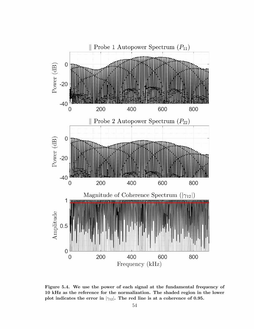
Figure 5.4. We use the power of each signal at the fundamental frequency of10 kHz as the reference for the normalization. The shaded region in the lowerplot indicates the error in |γ12|. The red line is at a coherence of 0.95.
54

PRF = 250 WPo = 4.5 mTorrfc,i = 200 kHz
(a) The gray region represents the theoretical predictions of the kineticplasma model from Eq. 4.3 for Te = 3− 6 eV, Ti = 0.25 eV, B0 = 526 G,and the measured k‖.
PRF = 250 WPo = 4.5 mTorrfc,i = 200 kHz
(b) The negative value of the kr‖ indicate that the wave travels in thedirection opposite to the background magnetic field.
Figure 5.5. All measurements have |γ12| > 0.95 with an error less than 0.05.
55

did not hinder the AWPI diagnostic’s ability to measure kr, but it did cause the ki
measurements to have far too much error to provide insight into the wave physics.
5.3 Discussion
The results represent an encouraging demostration of a proof-of-concept experiment
for the AWPI technique. However, we have encountered limited repeatability with
the excitation of electrostatic modes, regardless of whether we send harmonically-
rich or sinusoidal signals to the antenna. More often than not, for experimental
reasons yet to be determined, the measured dispersion relation has (1) phase velocities
ωr/kr ≈ c cS, which implies that the probes are AC coupled (i.e. coupling to long-
wavelength electromagnetic modes), or (2) dωr/dkr⊥ cS with ω(k⊥) 6= ω(−k⊥)
(i.e. no excitation of electrostatic modes, see note after Eq. 4.3). This difficulty with
successfully coupling to electrostatic modes is why we do not have accompanying
measurements of k‖ in the argon plasma. However, in all cases where electrostatic
modes were detected, the dispersion relation measurements were consistent with EIC
wave modes and resemble the data of Figs. 5.2 and 5.5.
5.4 Chapter Summary
In this chapter we presented our measurements of the dispersion relation of electro-
static ion-cyclotron waves taken with the AWPI diagnostic both in argon and helium
plasmas. These measurements agree over a wide range of frequencies with fluid and
kinetic theory predictions, respectively, which we calculated using the representative
plasma parameters for our RF source. The results demonstrate the diagnostic’s ability
to take expedited measurements of dozens of wavenumbers across different frequency
ranges.
56

Chapter 6
Conclusions
In this dissertation, we presented the Active Wave Packet Injection (AWPI) diagnos-
tic, a probe-based diagnostic used to measure dispersion relations in low-temperature
plasmas. This diagnostic improves past active wave injection techniques by using
harmonically-rich excitation signals to expedite the measurement of wavenumber as
a function of frequency. We showcased the diagnostic’s capabilities by manufacturing
and integrating a proof-of-concept prototype into a magnetized RF plasma source
to measure the dispersion relation of electrostatic ion-cyclotron waves in argon and
helium.
6.1 Summary of Contributions
The AWPI diagnostic, though intrusive in nature, provides a generalizable technique
to take expedited measurements of dispersion relations in plasmas. The harmonic
comb generating circuit is easily adapted to produce harmonics in a variety of fre-
quency ranges by simply changing the high-pass filter’s cutoff frequency and the
input square wave’s fundamental frequency. Different antenna and probe designs can
be implemented to excite and detect different types of wavemodes (e.g. electrostatic
vs. electromagnetic or ion vs. electron waves). The ability to measure wavenumbers
57

at multiple frequencies simultaneously is particularly attractive for pulsed plasma ex-
periments or experiments in which only limited exposure to the plasma environment
is possible before damage occurs (e.g hollow cathode plasmas).
Our investigation of electrostatic ion-cylotron waves in a magnetized RF plasma
source demostrated the AWPI diagnostic’s versatile wave-shaping characteristics and
compatibility with different gases. We measured the perpendicular propagation and
decay of EIC waves in an argon plasma over six harmonics of the ion-cyclotron fre-
quency. With a simple change to the circuit design, we also measured the perpendic-
ular and parallel propagation of EIC waves in a helium plasma over two harmonics
of the ion-cyclotron frequency. These measurements not only matched fluid and ki-
netic theory predictions, respectively, but also had a higher frequency resolution than
previous work and were each obtained in a single shot.
6.2 Recommendations for Future Work
Our difficulty coupling to electrostatic modes in the RF plasma merits for a detailed
investigation of broadband antenna designs for the AWPI diagnostic. While there is
well-established RF matching theory to tune antennas to plasma loads [6, 101], the
AWPI diagnostic requires simultaneous matching at more than one [40] or two [45]
frequencies. This may be accomplished with advanced matching techniques or by
exploring the effect of antenna geometry on coupling. This is also something to
consider if the diagnostic is applied to real thruster systems in which the physical
presence of the antenna and probes should not perturb the plasma. This means
that the physical scale of the diagnostic and the frequency range probed should be
appropriately scaled with respect to plasma parameters (e.g. electron Debye length
or ion plasma frequency in our case) to ensure proper interpretation of the data.
Our two-blade antenna geometry is adequate for the scale of our RF source and
58

perhaps the plume regions of plasma thrusters, but redesign would be necessary if
the diagnostic were used, for example, near the channel exit of a Hall effect thruster.
59

Appendix A
LIF Data Reduction
A.1 fi0 Measurements: Ion Temperature and Drift
Using the LIF technique to resolve the background ion velocity distribution function
fi0, we can determine both ion temperature and drift velocity in the direction parallel
to the axis of the laser beam [9, 52, 43]. Consider the one-dimensional distribution
function for a Maxwellian ion population in local thermal equilibrium,
fi0(v) =ni√
2π vth,ie−
(v−vd,i)2/2v2
th,i , (A.1)
where vth,i =√Ti/mi is the ion thermal velocity and vd,i the ion drift velocity. Sweep-
ing the laser frequency νL about the atomic electron trasnsition frequency ν0 in a
plasma with this fi0 yields a Gaussian fluorescent intensity profile described by
I0(ν) =β√
2π vth,ie−
(ν−ν)2/2σ2, (A.2)
with peak position ν = ν0 (1 + vd,i/c), width σ = ν0 vth,i/c, and β a constant that
depends on laser beam power, geometrical factors, and the attenuation of the collected
60

light. We calculate the ion drift velocity and ion tempertature by fitting I0 to the
measured fluorescent signal and backing out its peak position and width, respectively.
A.2 fi1 Measurements: Plasma Dispersion Rela-
tion
If a traveling electrostatic wave with frequency ω is present in the plasma, the com-
pressions and rarefactions of plasma density produce a time-dependent perturbation
fi1 to the background distribution function [54, 63]. This perturbation causes the
fluorescent signal to have two components (in-phase IIP and out-of-phase IQ with
respect to the wave) oscillating at ω. We can use the LIF technique to resolve both f1
components to yield wave dispersion relation measurements. We first model the effect
of the electrostatic wave on the ion distribution function using the Vlasov equation
for ion motion
∂fi
∂t+ v · ∂fi
∂x+
e
mi
(E + v ×B) · ∂fi
∂v= 0, (A.3)
where the electric and magnetic fields E and B have both background (0th order)
and perturbation (1st order) components. We consider the case with E0 = 0 and,
since the wave is electrostatic, E1 = −ikΦ1ei(k·x−ωt) and B1 = 0. Substituting into
the above equation and asssuming a three-dimensional magnetized Maxwellian back-
ground distribution function
fi0(v) = ni
(1
2πv2th‖
)1/2
e−(v‖−vd)2/2v2
th‖
(1
2πv2th⊥
)e−v2⊥/2v2
th⊥ , (A.4)
we obtain the first order equation
∂f1
∂t= i
qiφ1
mi
ei(k·x−ωt) k · ∂f0
∂v(A.5)
61

for the perturbation f1. This equation is solved through the method of characteristics
to yield an expression for f1(v) [31]. Since the LIF diagnostic only resolves velocities
in one spatial dimension (say x), we integrate the full expression for f1(v) over vy
and vz, giving the result f1(vx) = f1(vx)ei(k·x−ωt), where
f1(vx) =qiφ1
πmiv2th⊥,i
f0(vx)∑n,m
(1 + Z(ζn+m)ζ0
)Jm
(k⊥vxωc,i
)×e−imπ/2ei(m+n)θe
ik⊥ sin θvx/ωc,ie−a2/8e−
g2/4∑l
I(n+l)/2
(a2
8
)Il
(ag2
)eilπ/2
(A.6)
with a =√
2k⊥vth⊥,i/ωc,i, g =√
2k⊥ cos θ vth,i/ωc,i, θ = tan−1(ky/kx), Jm(x) the nth
order Bessel function of the first kind, and the rest of the symbols as defined in
Eq. 4.1. The real and imaginary parts of f1 are related to the in-phase(IIPmeas
)and
out-of-phase(IQmeas
)measurements of fluorescent intensity, respectively. We can fit
the analytical expression in Eq. A.6 to laser frequency sweeps of both components of
the fluorescent intensity and determine the best fit values of the free parameters k⊥
and θ, thereby measuring the dispersion relation of the electrostatic wave. Appendix
A.3 details the data reduction and error analysis we follow in the fitting procedure,
including considerations for the other free parameters φ1 and k‖, data phase correction
and normalization, and the inverse χ2 metric we use to evaluate the goodness of the
fit [54, 102].
A.3 f1 Data Reduction and Error Analysis
We follow the procedure outlined in Refs. [54, 43] to make dispersion relation measure-
ments of electrostatic plasma waves using the LIF diagnostic. The data processing for
determining k⊥ and θ involves three steps: (1) data phase correction, (2) free param-
eter reduction, and (3) goodness-of-fit evaluation. The data sets processed are the
in-phase and out-of-phase measurements of fluorescent intensity as a function of laser
62

frequency. While IIPmeas and IQmeas are real quantities, we define Imeas = IIPmeas + i IQmeas
for convenience during the data processing.
Since a phase difference ϕ exists between the source signal used as the LIA’s ref-
erence and the locally measured plasma density fluctuations, the collected fluorescent
intensity profiles exhibit a phase dependence Imeas ∝ eiϕf1 which we must remove
before applying the theoretical model from Eq. A.6. We calculate the phase as [54]
ϕ = tan−1
∫IQmeas dν∫IIPmeas dν
(A.7)
and multiply Imeas by a factor of e−iϕ to produce the phase-corrected data sets Imeas,c.
The real and imaginary parts of the analytical expression for f1 provide a system of
two equations to which to fit our two corrected data sets IIPmeas,c and IQmeas,c. However,
the fitting is underdetermined as there are four free parameters: k⊥, k‖, θ, and φ1. To
remedy this, we first note that φ1 appears only as a multiplicative prefactor in Eq. A.6,
so normalization of the intensity data and fitting function removes its presence. We
find the largest absolute value of IIPmeas,c and the frequency νmax at which it occurs. We
choose to normalize the data by the largest absolute value of the in-phase component
so that
Imeas,c(ν) =Imeas,c(ν)∣∣IIPmeas,c(νmax)
∣∣ . (A.8)
We correspondingly normalize our fitting function to define
f1(vx) =f1(vx)∣∣<f1(vx,max)
∣∣ , (A.9)
where vx,max = cν0
(ν0 − νmax) by Eq. 2.3. To account for k‖, we note that we can
solve the electrostatic dispersion relation in Eq. 4.1 to calculate k‖ as a function of
k⊥, leaving only k⊥ and θ as free parameters for fitting f1 to Imeas,c.
63

We search (k⊥, θ) space for the point which gives the best parameters to fit the
data. The metric we employ to find said parameters consists of a χ2 analysis that
evaluates how well f1(vx) matches Imeas,c(ν) given measurement error σ [102]. For
each (k⊥, θ) point considered, we calculate
χ2 =N∑p=1
1
σ2(p)
∣∣∣f (p)1 (vx)− I
(p)
meas,c(ν)∣∣∣2 (A.10)
over all collected wavelength points, with each σ(p) the sum in quadrature of the
error of the in-phase and out-of-phase components of the fluorescent intensity and N
the number of wavelengths sampled. Plotting 1/χ2 in the (k⊥, θ) space sampled we
identify the best fit parameters as the location of the peak of the distribution and
their uncertainty as the full width half maximum (FWHM) of the distribution.
64

Appendix B
Numerical Algorithms for Finding
and Tracking Complex Roots
To perform the procedure outlined in Sec. 2.2, we base our method for determining
the initial locations of the roots of D(ω,k) on previous work [86, 87] which took
advantage of the analytic (or meromorphic at worst) nature of dispersion relations
commonly encountered in plasma physics. We do not use any graphical methods for
this task; instead, we devise a root-searching protocol that only requires input from a
user at the start and has the potential for improved performance if implemented with
parallel programming practices. This provides the desired versatility for numerically
characterizing plasma waves and instabilities in arbitrary parameter spaces.
B.1 Global Root-Finding
Consider the meromorphic function f(z) and the analytic function g(z) over a simply-
connected open region R ∈ C. Assuming that f(z) is non-zero on the positively-
oriented closed contour Γ which bounds R (see Fig. B.1), Cauchy’s Argument Prin-
65

ciple states that [103]
1
2πi
∮Γ
g(ζ)f ′(ζ)
f(ζ)dζ =
∑k
mkg(zk)−∑p
dpg(zp), (B.1)
where zk and zp are the roots and poles of f(z) contained in R with multiplicities mk
and dp, respectively. If R does not contain any of the poles of f(z), then the above
summation over p disappears, which when combined with the choice g(z) = zt allows
us to define the contour integral
It =1
2πi
∮Γ
ζtf ′(ζ)
f(ζ)dζ =
∑k
mkztk. (B.2)
For the case t = 0, the integral gives the sum of the multiplicities of the roots contained
in R. If the region contains only one root, then for the case t = 1 the integral gives
the value of the root times its multiplicity. Note that if R only contains a simple root
of f(z), then I0 = 1 and I1 is the value of that root.
For our application, the function f(z) corresponds to a dispersion relation
D(ω,k; pi) after restricting it to a function of a single parameter as discussed in
Section 2.2. For example, the function
D[0](ω) = D(ω,k; pi)∣∣∣k[0],p
[0]i
(B.3)
would subsitute in for f(z) above in order to search for the location of the roots
ω[0](k[0]; p[0]i ) in the complex ω-plane. The poles of many D(ω,k; pi) studied in
plasma physics can be analytically removed from D or located beforehand in complex
plane [104, 31], ensuring only roots contribute to It, as written in Eq. B.2. Unfor-
tunately, it is unlikely that detailed enough a priori knowledge about the possible
value of each root is at hand to choose contours Γ that enclose only one root (if it
were, this whole procedure of global root-finding would not be needed). Moreover,
66

Re(z)
Im(z)
Γ
Rz1
z2
z3×z4
×z5
Figure B.1. The roots (•) and poles (×) of f(z) are located on the complexz-plane. The contour Γ, which delimits R, encloses two roots (z1, z2) and onepole (z4), so only these will contribute to the value of the integral in Eq. B.1.
the dispersion relations studied in plasma physics can commonly have an unknown
(possibly infinite) number of complex roots, so it is not even clear how many roots
might be present in the region of (ω,k)-space of interest.
Given these challenges, we design PRINCE to autonomously determine the num-
ber of roots in a region R and calculate initial estimates for their locations. PRINCE
conducts the search-and-refine procedure described in Section B.3 to focus down on
the location of a single root (whether simple or degenerate) by evaluating the contour
integral in Eq. B.2 and using a series of criteria to determine whether (1) a single root
has been found or (2) the region R needs to be divided into smaller subregions in
order to isolate the roots contained in it. For simplicity, we illustrate the procedure
for the specific case of Eq. B.3, though PRINCE can also handle the cases where
any one of the components of k is left as the independent variable for the dispersion
67

relation (e.g. f(z) is D(ky) by simplifying D(ω,k; pi) using initial values for ω, kx, kz,
and the pi).
B.2 Specification of Initial Search Region
The choice for the initial region R over which to search for roots of a dispersion rela-
tion depends on the physics to investigate. Typically, target frequency or wavelength
ranges based on physical considerations restrict the real values of ω or k (for exam-
ple, only looking at waves with frequencies in the MHz range or with wavelengths
smaller than the system dimensions). Similarly, the types of modes to study restrict
the imaginary component of ω or k. These could be purely propgating modes (in
which no energy exchanges between the wave and the plasma), damping modes (in
which the wave deposits energy into the plasma), or growing modes (in which the
wave extracts energy from the plasma). Fig. B.2 exemplifies the different regions
over which PRINCE searches for roots in the complex ω-plane based on the type of
modes investigated. Since Eq. B.1 assumes that f(z) is non-zero on the contour Γ,
the presence of purely propagating or purely evanescent modes (which correspond to
roots located on the real axis or on the imaginary axis, respectively) precludes us
from using contours that lie on the coordinate axes. While indenting the contour Γ
about the root remedies this problem analytically [103], such a strategy is not viable
for PRINCE since we do not know beforehand whether a root lies on the contour. In-
stead, we offset the contour from the axes when necessary by 1% of the upper bound
for ω or k.
Alternatively, non-relativistic and quasi-neutrality considerations (which are com-
monly applicable to plasma thruster discharges) can determine the extent of the search
region in the real and imaginary directions if no other bounds are otherwise speci-
fied. For a search in the complex ω-plane, PRINCE bounds R above by roughly
68

Re(ω)
Im(ω)
(a) Growing
Re(ω)
Im(ω)
(b) Growing and purelypropagating
Re(ω)
Im(ω)
(c) Damping
Re(ω)
Im(ω)
(d) Damping and purelypropagating
Re(ω)
Im(ω)
(e) Purely propagating
Re(ω)
Im(ω)
(f) All
Figure B.2. The different types of initial search regions correspond to searchesfor different types of modes. The offsets from the axes are exaggerated forclarity. The classification of stable or unstable for this example of roots in thecomplex ω-plane corresponds to the normal mode convention from Eq. 1.3.
69

non-relativistic particle motion over an electron Debye length, i.e. ωλD,e ≤ c. For a
search in the complex k-plane, PRINCE bounds R above such that the corresponding
wavelength is greater than the local Debye length, i.e. |k| = 2π/λ ≤ 2π/λD,e.
B.3 Algorithm Implementation
Once the initial search region has been defined, the algorithm to find the number and
locations of the initial roots of a dispersion relation D(ω) is as follows [86]:
1. Divide the search region R in the complex ω-plane into rectangular cells.
2. For each cell, evaluate I0 numerically along the delimiting contour.
3. For each cell, take one of three actions based on the value of I0:
(a) If Re(I0) = 1 within tolerance, a simple root was found, so calculate and
store I1 as the estimate for its location.
(b) If Re(I0) = 0 within tolerance, no roots are contained in the cell, so
disregard it.
(c) If |Re(I0)| > 0 and |1−Re(I0)| > 0 within tolerance, the cell may contain
unresolved roots, so label the cell as suspect.
4. If there are no suspect cells, all roots contained in R were found and the search
terminates. Otherwise, for each suspect cell there are two options:
(a) If D (I1/Re(I0)) = 0 within tolerance, the cell contains a single degenerate
root with multiplicity Re(I0), so store I1/Re(I0) as the estimate for its
location.
(b) If D (I1/Re(I0)) 6= 0 within tolerance, the suspect cell contains unresolved
roots, so recursively apply the algorithm to the cell.
70

Re(ω)
Im(ω)
A B
C D
ω1
ω4
ω2
ω3
Re(ω)
Im(ω)
ω1
ω4
ω2
ω3
0th Recursion Step 1st Recursion Step
Figure B.3. PRINCE determines in the 0th Recursion Step that cells C and Dcontain no roots while cell A only contains root ω1. Cell B is suspect, so it issubdivided into smaller cells in the 1st Recursion Step to resolve roots ω2 andω3. As root ω4 is not inside any of the search cells, it is ignored.
All tolerances are set to 0.01, i.e. Re(I0) = 1 is within tolerance if |Re(I0)− 1| < 0.01.
Figure B.3 illustrates this procedure for the example of four zeros, three of which
correspond to physically-relevant linearly unstable wavemodes. The sign of the real
part of the root indicates whether the wave’s phase velocity is parallel or anti-parallel
to k. The initial search region R is the union of the four disjoint rectangular regions,
one in each quadrant of the complex plane and each off-set from the real and imaginary
axes by the predefined distances discussed in Section B.2. PRINCE recursively applies
the search algorithm only to the suspect cells containing unresolved roots (Cell B in
this example). The other cells are discarded once the number and locations of any
resolved roots are stored.
71

B.4 Iterative Local Root-Tracking
The global root-finding algorithm determines the number of roots contained in R
and estimates their values for the initial set of conditions k[0] and p[0]. With this
information, a more efficient root-finding algorithm (the Newton-Raphson method in
PRINCE) can now be used to calculate the value of the roots as we iteratively vary
one of the wave parameters away from these initial conditions. For example, once
the roots ω[0]j of D[0](ω) = D(ω,k[0]; p
[0]i ) are located, we can track their location in
the complex ω-plane as we vary kx away from k[0]x . At the nth step of the iteration,
we first re-evaluate the dispersion relation for the new value k[n]x to obtain D[n](ω).
To find the new locations ω[n]j of each root, we use ω
[n−1]j as the initial guess for
the root-finding algorithm. The procedure based on complex integration described
in the previous section could be applied again, but its computation is significantly
more costly, particularly compared to the Newton-Raphson method. This iteration
produces a numerical characterization of each wavemode ωj(kx) that was initially
found.
72

Appendix C
Plasma Rocket Instability
Characterizer1
In this appendix we describe the initial implementation of the Plasma Rocket
Instability Characterizer (PRINCE), an interactive software tool which enables the
numerical characterization of plasma waves’ and instabilities’ dependence on plasma
parameters across relevant frequency or wavenumber domains. We describe the
frontend graphical user interface (GUI) which allows for versatile data input and
parametric control of the search parameters. We also present a proof-of-concept
reproduction of previous work which studied unstable Esipchuk-Tilinin wavemodes
present in Hall effect thrusters to validate the performance of PRINCE.
C.1 Frontend Graphical User Interface
We integrate the procedures described in the previous appendix into a software pro-
gram written in Wolfram’s Mathematica 10.4. While other platforms or coding lan-
1This chapter is based on work previously presented in [105]: Rojas Mata, S., Choueiri, E. Y.,Jorns, B. A., and Spektor, R., ”PRINCE: A Software Tool for Characterizing Waves and Instabilitiesin Plasma Thrusters,” 52nd AIAA/SAE/ASEE Joint Propulsion Conference, Salt Lake City, UT,2016.
73

guages provide better computational performance, we made a trade-off between op-
timal computational power and the built-in ease for GUI design and analytical ma-
nipulations which Mathematica provides. The resulting 3-panel interactive interface
controls the input of the specific dispersion relation D to study, the region in (ω,k)-
space to search for roots, and the plasma parameters pi.
C.1.1 Plasma Parameters Panel
The import of the plasma parameters pi is done through the panel shown in Fig. C.1.
Each plasma parameter available has a small unfolding menu for specifying spatial
dependencies and the filepath to access the data files. If the plasma parameter does
not have a spatial dependence (0D), then just a value input box appears. Whether
the input of a particular parameter is necessary or optional depends on the dispersion
relation chosen (see Section C.1.2). Fig. C.2 shows the different levels of the parameter
menus for one- or two-dimensional spatial dependencies. Checking a parameter’s box
will select the parameter for import. The information requested in the menu must
be specified for proper import of the data (see below for formatting notes); if not,
an error dialog will appear when the ‘Import’ button is pressed. Each ‘Clear’ button
clears all import information for that parameter. Unchecking the check box removes
the parameter from import but does not clear any specified information.
For each plasma parameter checked, the following must be specified:
Dimensionality: what the spatial dimensionality of the data is
Variable dependence: on which Cartesian variables does the data depend
Filepath: where in the computer is the data stored
In addition to the plasma parameters, the gas and the units of the spatial coordi-
nates are selected in this panel. If all necessary information is specified, pressing the
‘Import’ button on the bottom right will read the data into PRINCE and display
74

Figure C.1. PRINCE offers several dimensionality and Cartesian-coordinate-dependence options for fourteen different input plasma parameters. The useralso specifies the units of the input spatial discretization as well as the gas.
Dimensionality
Variables File path
Figure C.2. The user must specify all fields in order to import the file.
a success dialog. Otherwise, an error dialog detailing the missing information will
appear.
If the plasma parameter has no spatial dependence (0D dimensionality), only
a scalar value needs to be provided in the input value field.2 If there is a spatial
dependence, then the data file must be a CSV text file where the last column is the
parameter values and the preceding columns (one for a 1D dependence or two for
a 2D dependence) are the spatial coordinate values. For 2D data, the order of the
variables in the columns of the data file must match the order of the variables selected
in the variable dependence section of the menu. So, if the variable dependence chosen
is “x, z”, the first column in the data file should be the x-coordinate values and the
2Note that Mathematica does not recognize “E” notation for order of magnitude. Instead anumber like 5× 10¹⁸ needs to be input as 5*10ˆ18, not 5E18.
75

second the z-coordinate values. The number of coordinates and their values in any
one direction must be the same for all parameters which depend on that direction;
PRINCE is not designed to interpolate or extrapolate values for missing coordinate
points. The units of the parameter must match those displayed in the header of the
parameter’s menu (e.g. eV for ion or electron temperature).
C.1.2 Solver Settings Panel
The dispersion relation to study is selected in the panel shown in Fig. C.3. The
dropdown menu contains the following pre-programmed dispersion relations:
Simplified Esipchuk-Tilinin waves
Long wavelength gradient drift waves
High-frequency E×B drift waves
Damped warm Langmuir waves
(Simplified) Magnetized electrostatic waves in a warm plasma
Low-frequency MHD waves
Forward electrostatic ion-cyclotron waves
Electrostatic ion acousitc modes
There is also an option for a user-specified dispersion relation which is easily defined
in an auxiliary file (see Appendix D). Each pre-programmed dispersion relation dis-
plays in red until all the necessary plasma parameters are checked in the ‘Plasma
Parameters’ panel. The necessary and optional parameters or gradients of parame-
ters display in the box to the right of the dispersion relation. To the left is a graphical
depiction of the coordinate geometry and vector fields selected which provides a check
that the spatial configuration of the system is set up correctly.
76

In the bottom half of the panel, the bounds for the search region in the complex
plane and details of the iteration process are specified. PRINCE can either solve
for complex values of ω over an iteration of real values of one of the k components
or for complex values of one of the k components over an iteration of real values
of ω. The iteration variable as well as its range and resolution should be specified
first. An iteration over ω requires specification of which component of k to solve for;
similarly, an iteration over a k component requires specification of which component
to iterate over. Both options leave two of the three k components as free parameters,
so their values must be specified either as constant or propotional to the third solved
for/iterated over component. The labels in the panel dynamically update as the
choices are made to provide clarity in the process. In the bottom left corner, the
bounds for the real and imaginary parts of the solved for variable are specified to define
Reference coordinate system D(ω,k; pi) selection Parameter requirements
Search region boundsIteration variable, free k-componentvalues, and mode types specification
Figure C.3. The user specifies the dispersion relation to study from the drop-down menu and the details of the (ω,k)-space sweep in the various fields.
77

the initial search region. Alternatively, automatic limits based on quasineutrality and
relativistic considerations can be used (see Section B.2).
The final step is to choose which types of modes to search for: purely propagating,
growing, damping, or a combination of these. The sign convention used to define
whether wavemodes are growing or damping is that of Fourier modes of the form
exp[i(k ·x−ωt)] (see Eq. 1.3). This means that modes with a positive ωi are growing
modes while damping modes have the opposite signature. Analogously, modes with
a negative ki are growing modes while damping modes have the opposite signature.
Purely propagating modes have ωi = ki = 0. The signature of either ωr or kr indicate
the direction of propagation relative to the coordinate system used.
Once all the necessary information in this panel is set, pressing the ‘Solve’ but-
ton starts the search for all the roots of the dispersion relation located inside the
specified complex-plane region at each spatial coordinate point. If there is an error
with the input information an error dialog will appear detailing the problem. Once
the global root-finding procedure resolves all the roots in the search region, the local
root-tracking routine characterizes each one of them as a function of the iteration
variable. Progress dialogs continuously display as PRINCE computes until a final
completion dialog appears.
C.1.3 Data Visualization Panel
This bottom panel provides some simple plotting routines to study results. In the
‘Heat Maps’ section, the ‘Binary Instability Spatializer’ button brings up a spatial
heat map that indicates at which grid points instabilites were found i.e. coordinate
points where Im(ω) > 0 or Im(k) < 0. The ‘Dominant Unstable Mode’ buttons bring
up spatial heat maps of the real part of either the wavenumber or frequency of the
unstable mode with biggest growth rate at each coordinate point.
78

In the ‘Single Branch Options’ section, pressing the ‘Output Results’ button cre-
ates a new subdirectory to export the results of the characterization for each root.
The data file names begin with the spatial coordinates where the root was found fol-
lowed by a “ BX” suffix where the X denotes the branch number of the root. The files
are CSV text files where the first column contains the values of the iteration variable,
the second column contains the real part of the root, and the third column contains
the imaginary part of the root. Once the raw data has been output, the ‘Plots’ button
in the ‘Single Branch’ section allows the user to plot the real and imaginary parts of
a root as a function of the iteration variable.
C.2 Validation of PRINCE
C.2.1 Esipchuk-Tilinin Dispersion Relation Study
We validate PRINCE by reproducing previous work [11] which investigated instabil-
ities arising in a Hall effect thruster channel from solutions to the Esipchuk-Tilinin
dispersion relation [106]
1
ω2p,i
− 1
(ω − kxvd,i)2+
1
ωc,eωc,i+
1
k2⊥v
2A
− ky(ude − uB)
k2⊥v
2d,i(ω − kyude)
= 0. (C.1)
Here ωp,i is the ion plasma frequency, vd,i the axial ion drift velocity, ωc,e and ωc,i
the electron and ion cyclotron frequencies, vA the Alfven velocity, ude the azimuthal
E×B electron drift velocity, and uB the magnetic drift velocity. Ref. [11] restricted the
frequency range considered such that (ω−kxvd,i)2 ωc,eωc,i ω2p,i and (ω−kxvd,i)2
k2⊥v
2A to simplify the dispersion relation to
1
(ω − kxvd,i)2+
ky(ude − uB)
k2⊥v
2d,i(ω − kyude)
= 0, (C.2)
79

so this is the version we analyze with PRINCE. Extracted experimental data sets
with xenon as propellant [107] with a spatial resolution of 1 mm for electron density,
electric potential, and radial magnetic field, reproduced in Fig. C.4(a)-(c), served as
the input to calculate vd,i, ude = −Ex/Bz, ωc,i = eBz/mi, and uB = ∂Bz∂xvd,i/ωc,i in
both the previous work and our reproduction.
C.2.2 Procedure and Results
Ref. [11] characterized instabilities arising in the mostly azimuthal propagation (ky =
10kx) of the mode with k⊥ =√k2x + k2
y = 1/z, where z is the local radius of curvature
of the channel (refer to Fig. 1.2). The results comprise computations of the complex
roots ω(kx, ky) using the analytical solution of Eq. C.2. Fig. 9(f) in Ref. [11] plots the
real part of the roots at the locations where the root has a positive imaginary part,
signifying that the mode is unstable. To reproduce this analysis, we use PRINCE to
numerically characterize the zeros ω(k) of Eq. C.2. We set kz = 0 and ky = 10kx
and vary kx between 2 /m and 4 /m at a resolution of 0.05/m. We extract the
value of ω corresponding to the mode k⊥ = 1/z for each spatial point from the raw
output data to produce Fig. C.4(d), our reproduction of Fig. 9(f) from Ref. [11]. The
locations where instabilities arise match well, corresponding as expected to the region
in the channel where the radial magnetic field gradient is negative with respect to
the axial variable (∂Bz/∂x < 0). The frequency range (20-50 kHz) is also comparable,
differences no larger than 10 kHz potentially due to different interpolation schemes
used to calculate the gradients and secondary plasma quantities.
80

ElectronDensity,1017/m
3
02
46
010
20
30
40
25
30
35
40
45
50
DownstreamAxialPosition,mm
ChannelRadius,mm
ElectricPotential,V
025
50
75
100
125
010
20
30
40
25
30
35
40
45
50
DownstreamAxialPosition,mm
ChannelRadius,mm
010
20
30
40
0
50
100
150
DownstreamAxialPosition,mm
RadialMagneticField,G
FrequencyofUnstableModes,kHz
010
20
30
40
010
20
30
40
25
30
35
40
45
50
DownstreamAxialPosition,mm
ChannelRadius,mm
(a)
(b)
(c)
(d)
Fig
ure
C.4
.P
rofi
les
of
the
ele
ctr
on
den
sity
,ele
ctr
icp
ote
nti
al,
an
dra
dia
lm
agn
eti
cfi
eld
extr
acte
dfr
om
Ref.
[107]
dis
pla
yin
pan
els
(a),
(b),
an
d(c
),re
specti
vely
.T
he
real
frequ
en
cy
of
the
un
stab
lem
od
es
of
Eq.
C.2
wit
hk⊥
=1/z
an
dm
ost
lyazim
uth
al
pro
pagati
on
(ky
=10kx)
are
dis
pla
yed
inp
an
el
(d).
Blu
ed
en
ote
sst
ab
lere
gio
ns.
81

Appendix D
PRINCE Examples
In this appendix we provide two examples of using PRINCE to characterize a pre-
programmed or custom dispersion relation with sample data sets. These data ex-
tracted from Ref. [107] are axial profiles at constant radius of xenon plasma properties
inside the channel of a Hall thruster.
D.1 Pre-Programmed Dispersion Relation: Esipchuk-
Tilinin
Equation in red until necessaryparameters are selected
Figure D.1. Esipchuk-Tilinin Dispersion Relation Display
82

Figure D.2. Data Import for Esipchuk-Tilinin Example
In this example we will characterize wave modes arising as solutions to a simplified
version of the Esipchuk-Tilinin dispersion relation [106, 11]. Instead of considering
the cylindrical geometry of the thruster, this model uses a Cartesian system with
r → z, θ → −y, z → x. Choosing this dispersion relation from the drop down menu
indicates that the necessary parameters are plasma density, electric potential (and its
gradient in x), ion drift velocity in x, and magnetic field in z, as seen in Fig. D.1. A
gradient in x for the magnetic field is an optional parameter which will change the
form of the dispersion relation. We input the sample data files through the “Plasma
Parameter” panel as seen in Fig. D.2. Note that the electron temperature data is not
necessary for this dispersion relation but may be input anyway. The propellant gas
is xenon and the grid units are millimeters.
Following the analysis of Ref. [11], we will solve for ω as a function of kx for
primarily azimuthal modes with ky = 10kx and kz = 0. We iterate kx over the range
1-100 m-1 with a resolution of 0.1 m-1. For this example we want to characterize
growing wave modes in the low kHz range, so we set the search domain limits between
1 kHz and 100 kHz. Fig. D.3 shows these settings input into PRINCE.
83

Figure D.3. Solver Settings for Esipchuk-Tilinin Example
The results of this analysis are displayed in the figures below. The “Binary In-
stability Spatializer” shows that unstable modes were found around x = 44 mm (see
Fig. D.4). Clicking on the “Dominant Unstable Mode” buttons indicates that there
are three grid points with unstable branches. Outputting the results and using the
“Single Branch” plotter for the first (and only) branch of point x = 44 mm gives the
dispersion relation shown in Fig. D.5.
Figure D.4. Locations of Unstable Modes
84

Figure D.5. Example Dispersion Relation for Branch at x = 44 mm.
D.2 User-Specified Dispersion Relation
Custom dispersion relations can be input using the template found in the “Cus-
tom Relation.nb” file. This notebook should be edited and ran after the main
“PRINCE.nb” notebook has been run. The “Custom Dispersion Relation” option in
the drop down menu will use the function coded in the template notebook (though
it will not display the function input by the user).
At the top of the document are the physical constants coded in PRINCE. Any
other constants needed should be declared there with their values in SI units. Then
there are three editing steps for the contents of the Block:
1. Store any input plasma parameter or gradient used in a local variable inside the
function
2. Define additional local variables for calculated plasma parameters
3. Write the dispersion relation function
85

Any local variables used must first be declared inside the curly braces at the beginning
of the Block. All lines of code must end with a semi-colon except the expression
defining the dispersion relation, which must be at the very end of the Block.
The template file comes with example local variables and an arbitrary function
declared. Note the format to access plasma parameters and gradient values, which
uses the string aliases listed at the end of the template file for reference. The pa-
rameter values are accessed through the params structure while gradients are accesed
through the gradMat structure. For example, to use the electron drift velocity in x we
would set a local variable equal to params[“udex”]. Similarly, if we wanted to use the
gradient of neutral density in z we would set a local variable equal to gradMat[“n0”,
“z”]. Note that the quotes around the arguments passed to params and gradMat are
necessary since the aliases should be strings.
For help implementing any mathematical functions in the expression for the dis-
persion relation please refer to the Mathematica documentation. Note that while
PRINCE provides a framework to numerically investigate arbitrary functions, there
is no guarantee that function evaluations will be quick or well-behaved numerically
in the region of (ω,k)-space surveyed.
86

Bibliography
[1] Vines, S. K., Allen, R. C., Anderson, B. J., Engebretson, M. J., Fuselier, S. A.,Russell, C. T., Strangeway, R. J., Ergun, R. E., Lindqvist, P. A., Torbert, R. B.,and Burch, J. L., “EMIC Waves in the Outer Magnetosphere: Observations ofan Off-Equator Source Region,” Geophysical Research Letters , Vol. 46, 2019,pp. 5707–5716.
[2] Ram, A. K., Bers, A., and Benisti, D., “Ionospheric ion acceleration by multipleelectrostatic waves,” Journal of Geophysical Research: Space Physics , Vol. 103,No. A5, 1998, pp. 9431–9440.
[3] Khotyaintsev, Y. V., Graham, D. B., Norgren, C., and Vaivads, A., “Colli-sionless Magnetic Reconnection and Waves: Progress Review,” Frontiers inAstronomy and Space Sciences , Vol. 6, No. 70, 2019, pp. 1–20.
[4] Chen, Q., Otto, A., and Lee, L. C., “Tearing instability, Kelvin-Helmholtzinstability, and magnetic reconnection,” Vol. 102, No. A1, 1997, pp. 151–161.
[5] Boswell, R. W. and Chen, F. F., “Helicons-The Early Years,” IEEE Transac-tions on Plasma Science, Vol. 25, No. 6, 1997, pp. 1229–1244.
[6] Chabert, P. and Braithwaite, N., Physics of Radio-Frequency Plasmas , Cam-bridge University Press, New York, 2014.
[7] Yamamoto, T., Imai, T., Shimada, M., Suzuki, N., Maeno, M., Konoshima,S., Fujii, T., Uehara, K., Nagashima, T., Funahashi, A., and Fujisawa, N.,“Experimental Observation of the rf-Driven Current by the Lower-Hybrid Wavein a Tokamak,” Physical Review Letters , Vol. 45, No. 9, 1980, pp. 716–719.
[8] Cairns, R. A., Radiofrequency Heating of Plasmas , A. Hilger, Bristol, England,1991.
[9] Hutchinson, I. H., Principles of Plasma Diagnostics , Cambridge UniversityPress, New York, 2002.
[10] Surko, C. M. and Slusher, R. E., “Waves and Turbulence in a Tokamak FusionPlasma,” Science, Vol. 221, No. 4613, 1983, pp. 817–822.
[11] Choueiri, E. Y., “Plasma Oscillations in Hall Thrusters,” Physics of Plasmas ,Vol. 8, No. 4, 2001, pp. 1411–1426.
87

[12] Jahn, R. G., Physics of Electric Propulsion, Dover Publications, Inc., Mineola,New York, 2006.
[13] Cappelli, M. A., Meezan, N. B., and Gascon, N., “Transport physics in Hallplasma thrusters,” 40th AIAA Aerospace Sciences Meeting and Exhibit , No.January, Reno, NV, 2002, pp. AIAA–2002–485.
[14] Janes, G. S. and Lowder, R. S., “Anomalous Electron Diffusion and Ion Ac-celeration in a Low-Density Plasma,” The Physics of Fluids , Vol. 9, No. 6,1966.
[15] Adam, J. C., Boeuf, J.-P., Dubuit, N., Dudeck, M., Garrigues, L., Gresillon,D. M., Heron, A., Hagelaar, G. J. M., Kulaev, V., Lemoine, N., Mazouffre, S.,Perez Luna, J., Pisarev, V., and Tsikata, S., “Physics, simulation and diagnos-tics of Hall effect thrusters,” Plasma Physics and Controlled Fusion, Vol. 50,No. 12, 2008, pp. 124041.
[16] Heeron, A. and Adam, J. C., “Anomalous conductivity in Hall thrusters: Ef-fects of the non-linear coupling of the electron-cyclotron drift instability withsecondary electron emission of the walls,” Physics of Plasmas , Vol. 20, No. 8,2013, pp. 82313.
[17] Spektor, R., “Quasi-Linear Analysis Of Anomalous Electron Mobility Inside AHall Thruster,” 30th International Electric Propulsion Conference, Florence,Italy, 2007, pp. 1–10.
[18] Martorelli, R., Lafleur, T., Bourdon, A., and Chabert, P., “Comparison betweenad-hoc and instability-induced electron anomalous transport in a 1D fluid sim-ulation of Hall-effect thruster,” Physics of Plasmas , Vol. 26, No. 8, 2019.
[19] Mikellides, I. G. and Lopez Ortega, A., “Challenges in the development andverification of first-principles models in Hall-effect thruster simulations that arebased on anomalous resistivity and generalized Ohm’s law,” Plasma SourcesScience and Technology , Vol. 28, No. 1, 2019.
[20] Jorns, B. A., Mikellides, I. G., and Goebel, D. M., “Ion acoustic turbulencein a 100-A LaB6 hollow cathode,” Physical Review E , Vol. 90, No. 6, 2014,pp. 063106.
[21] Litvak, A. A. and Fisch, N. J., “Resistive Instabilities in Hall Current PlasmaDischarge,” Physics of Plasmas , Vol. 8, No. 2, 2001, pp. 648–651.
[22] Lobbia, R. B., A Time-resolved Investigation of the Hall Thruster BreathingMode, Ph.D. thesis, University of Michigan, 2010.
[23] Ellison, C. L., Raitses, Y., and Fisch, N. J., “Cross-field electron transportinduced by a rotating spoke in a cylindrical Hall thruster,” Physics of Plasmas ,Vol. 19, No. 1, 2012.
88

[24] Koshkarov, O., Smolyakov, A., Raitses, Y., and Kaganovich, I., “Self-Organization, Structures, and Anomalous Transport in Turbulent PartiallyMagnetized Plasmas with Crossed Electric and Magnetic Fields,” Physical Re-view Letters , Vol. 122, No. 18, 2019, pp. 185001.
[25] Cavalier, J., Lemoine, N., Bonhomme, G., Tsikata, S., Honore, C., andGresillon, D., “Hall thruster plasma fluctuations identified as the E x B elec-tron drift instability: Modeling and fitting on experimental data,” Physics ofPlasmas , Vol. 20, No. 8, 2013, pp. 082107.
[26] Lafleur, T., Baalrud, S. D., and Chabert, P., “Theory for the anomalous electrontransport in Hall effect thrusters. I. Insights from particle-in-cell simulations,”Physics of Plasmas , Vol. 23, No. 5, 2016, pp. 053502.
[27] Brown, Z. A. and Jorns, B. A., “Spatial evolution of plasma waves in theacceleration region and near-field of a magnetically shielded hall thruster,” 2018Joint Propulsion Conference, 2018, pp. 1–12.
[28] Yoshikawa, S. and Rose, D. J., “Anomalous Diffusion of a Plasma across aMagnetic Field,” Physics of Fluids , Vol. 5, No. May 2015, 1962, pp. 334.
[29] Spitzer, L., Physics of Fully Ionized Gases , Dover Publications, Inc., Mineola,New York, 2006.
[30] Liewer, P. C. and Krall, N. A., “Self-consistent approach to anomalous resistiv-ity applied to theta pinch experiments,” The Physics of Fluids , Vol. 16, No. 11,1973.
[31] Stix, T. H., Waves in Plasmas , Springer, New York, 1992.
[32] Chen, F. F., Introduction to Plasma Physics , Plenum Press, New York, 1974.
[33] Goldston, R. J. and Rutherford, P. H., Introduction to Plasma Physics , Taylor& Francis Group, New York, 1995.
[34] Frias, W., Smolyakov, A. I., Kaganovich, I. D., and Raitses, Y., “Long wave-length gradient drift instability in Hall plasma devices. I. Fluid Theory,” Physicsof Plasmas , Vol. 19, No. 5, 2012, pp. 052108.
[35] Lominadze, D. G., Cyclotron Waves in Plasma, Pergamon Press, Oxford, 1981.
[36] Goree, J., Ono, M., and Wong, K. L., “Observation of the backward electrostaticion-cyclotron wave,” Physics of Fluids , Vol. 28, No. 9, 1985.
[37] Beall, J. M., Kim, Y. C., and Powers, E. J., “Estimation of wavenumber andfrequency spectra using fixed probe pairs,” Journal of Applied Physics , Vol. 53,No. 6, 1982, pp. 3933–3940.
89

[38] Ohnuma, T., Miyake, S., Sato, T., and Watari, T., “Propagation of Electrostaticion Waves Near Ion Cyclotron Harmonics,” Physical Review Letters , Vol. 26,No. 10, 1970, pp. 541.
[39] Skiff, F. and Anderegg, F., “Direct Observation of Plasma Dielectric Motion,”Physical Review Letters , Vol. 59, No. 8, 1987, pp. 896–899.
[40] Spektor, R. and Choueiri, E. Y., “Excitation and propagation of ElectrostaticIon Cyclotron waves in rf-sustained plasmas of interest to propulsion research,”40th AIAA/ASME/SAE/ASEE Joint Propulsion Conference and Exhibit , FortLauderdale, FL, 2004.
[41] Lieberman, M. A. and Lichtenberg, A. J., Principles of Plasma Discharges andMaterials Processing , John Wiley & Sons, New York, 2005.
[42] Boswell, R. W., “Plasma production using a standing helicon wave,” PhysicsLetters A, Vol. 33, No. 7, 1970, pp. 457–458.
[43] Kline, J. L., Scime, E. E., Keiter, P. a., Balkey, M. M., and Boivin, R. F.,“Ion heating in the HELIX helicon plasma source,” Physics of Plasmas , Vol. 6,No. 12, 1999, pp. 4767.
[44] Ikezi, H. and Taylor, R. J., “Observation of First-Order Ion Energy Distributionin Ion-Acoustic Waves,” Physical Review Letters , Vol. 22, No. 18, 1969, pp. 923–925.
[45] Jorns, B., Sorenson, R., and Choueiri, E., “Variable dual-frequency electro-static wave launcher for plasma applications,” Review of Scientific Instruments ,Vol. 82, No. 12, 2011.
[46] Smith, D. E., Powers, E. J., and Caldwell, G. S., “Fast-Fourier-transformspectral-analysis techniques as a plasma fluctuation diagnostic tool,” IEEETransactions on Plasma Science, Vol. 2, No. 4, 1974, pp. 261–272.
[47] Albarede, L., Mazouffre, S., Bouchoule, A., and Dudeck, M., “Low-frequencyelectron dynamics in the near field of a Hall effect thruster,” Physics of Plasmas ,Vol. 13, No. 6, 2006, pp. 1–7.
[48] Lazurenko, A., Dudok De Wit, T., Cavoit, C., Krasnoselskikh, V., Bou-choule, A., and Dudeck, M., “Determination of the electron anomalous mobilitythrough measurements of turbulent magnetic field in Hall thrusters,” Physicsof Plasmas , Vol. 14, No. 3, 2007.
[49] Stevens, J. E., Sowa, M. J., and Cecchi, J. L., “Helicon plasma source excitedby a flat spiral coil,” Journal of Vacuum Science & Technology A: Vacuum,Surfaces, and Films , Vol. 13, No. 5, 1995, pp. 2476–2482.
[50] Smy, P. R., “The use of Langmuir probes in the study of high pressure plasmas,”Advances in Physics , Vol. 25, No. 5, 1976, pp. 517–553.
90

[51] Lazurenko, A., Coduti, G., Mazouffre, S., and Bonhomme, G., “Dispersionrelation of high-frequency plasma oscillations in Hall thrusters,” Physics ofPlasmas , Vol. 15, No. 3, 2008, pp. 34502.
[52] Stern, R. A. and Johnson, J. A., “Plasma Ion Diagnostics Using ResonantFluorescence,” Phys. Rev. Lett., Vol. 34, No. 25, 1975, pp. 1548–1551.
[53] Severn, G. D., Edrich, D. A., and McWilliams, R., “Argon ion laser-inducedfluorescence with diode lasers,” Review of Scientific Instruments , Vol. 69, No. 1,1998, pp. 10.
[54] Sarfaty, M., De Souza-Machado, S., and Skiff, F., “Direct determination ofion wave fields in a hot magnetized and weakly collisional plasma,” Physics ofPlasmas , Vol. 3, No. 12, 1996, pp. 4316–4324.
[55] Jorns, B. A., Experimental Characterization of Plasma Heating with BeatingElectrostatic Waves , Ph.D. Dissertation, Princeton University, 2012.
[56] Jorns, B. A. and Choueiri, E. Y., “Stochastic Threshold for Ion Heating withBeating Electrostatic Waves,” Physical Review Letters , Vol. 110, No. 24, 2013,pp. 1–5.
[57] Saloman, E. B., “Energy levels and observed spectral lines of ionized argon,Ar II through Ar XVIII,” Journal of Physical and Chemical Reference Data,Vol. 39, No. 3, 2010.
[58] Moore, C. E. and Merrill, P. W., “Partial Grotrian Diagrams of AstrophysicalInterest,” 1968.
[59] Hill, D. N., Fornaca, S., and Wickham, M. G., “Single frequency scanning laseras a plasma diagnostic,” Review of Scientific Instruments , Vol. 54, No. 3, 1983,pp. 309–314.
[60] Hargus, W. A. and Cappelli, M. A., “Laser-induced fluorescence measurementsof velocity within a Hall discharge,” Applied Physics B: Lasers and Optics ,Vol. 72, No. 8, 2001, pp. 961–969.
[61] Keesee, A. M., Scime, E. E., and Boivin, R. F., “Laser-induced fluorescencemeasurements of three plasma species with a tunable diode laser,” Review ofScientific Instruments , Vol. 75, No. 10, 2004, pp. 4091–4093.
[62] Verreycken, T., Van Der Horst, R. M., Baede, A. H., Van Veldhuizen, E. M.,and Bruggeman, P. J., “Time and spatially resolved LIF of OH in a plasma fila-ment in atmospheric pressure HeH 2O,” Journal of Physics D: Applied Physics ,Vol. 45, No. 4, 2012.
[63] Kline, J. L., Franck, C., and Spangler, R., “First order perturbed velocitydistribution theory and measurement,” Tech. rep., West Virginia University,2000.
91

[64] Wagner, H. P., Kaeppeler, H. J., and Auweter-Kurtz, M., “Instabilities in MPDthruster flows: 1. Space charge instabilities in unbounded and inhomogeneousplasmas,” Journal of Physics D: Applied Physics , Vol. 31, No. 5, 1998, pp. 519–528.
[65] Frias, W., Smolyakov, A. I., Kaganovich, I. D., and Raitses, Y., “Long wave-length gradient drift instability in Hall plasma devices. II. Applications,”Physics of Plasmas , Vol. 20, No. 5, 2013, pp. 052108.
[66] Holzhauer, E. and Massig, J. H., “An analysis of optical mixing in plasmascattering experiments,” Plasma Physics , Vol. 20, No. 9, 1978, pp. 867–877.
[67] Tsikata, S., Lemoine, N., Pisarev, V., and Gresillon, D. M., “Dispersion re-lations of electron density fluctuations in a Hall thruster plasma, observed bycollective light scattering,” Physics of Plasmas , Vol. 16, No. 3, 2009.
[68] Tsikata, S., Honore, C., Lemoine, N., and Gresillon, D. M., “Three-dimensionalstructure of electron density fluctuations in the Hall thruster plasma: E x Bmode,” Physics of Plasmas , Vol. 17, No. 11, 2010.
[69] Delves, L. M. and Lyness, J. N., “A Numerical Method for Locating the Zerosof an Analytic Function,” Mathematics of Computation, Vol. 21, 1967, pp. 543–560.
[70] Ioakimidis, N. I. and Anastasselou, E. G., “A modification of the delves-lynessmethod for locating the zeros of analytic functions,” Journal of ComputationalPhysics , Vol. 59, No. 3, 1985, pp. 490–492.
[71] Pan, V. Y., “Solving a Polynomial Equation: Some History and RecentProgress,” Vol. 39, No. 2, 1997, pp. 187–220.
[72] Kowalczyk, P., “Complex Root Finding Algorithm Based on Delaunay Trian-gulation,” ACM Transactions on Mathematical Software, Vol. 41, No. 3, 2015.
[73] Hittle, D. C. and Bishop, R., “An Improved Root-Finding Procedure for Usein Calculating Transient Heat Flow through Multilayered Slabs,” InternationalJournal of Heat and Mass Transfer , Vol. 26, No. 11, 1983, pp. 1685–1693.
[74] Dunkel, J. and Weber, S., “Stochastic root finding and efficient estimation ofconvex risk measures,” Operations Research, Vol. 58, No. 5, 2010, pp. 1505–1521.
[75] Chun, S. and Kwasinski, A., “Analysis of classical root-finding methods appliedto digital maximum power point tracking for sustainable photovoltaic energygeneration,” IEEE Transactions on Power Electronics , Vol. 26, No. 12, 2011,pp. 3730–3743.
92

[76] Bagatur, T., “Modified Newton–Raphson Solution for Dispersion Equation ofTransition Water Waves,” Journal of Coastal Research, Vol. 23, No. 6, 2007,pp. 1588–1592.
[77] Dubbelday, P. S., “Application of a New Complex Root-Finding Technique tothe Dispersion Relations for Elastic Waves in a Fluid-Loaded Plate,” SIAMJournal of Applied Mathematics , Vol. 43, No. 5, 1983, pp. 1127–1139.
[78] Newman, J. N., “Numerical solutions of the water-wave dispersion relation,”Applied Ocean Research, Vol. 12, No. 1, 1990, pp. 14–18.
[79] Ugincius, P. and Uberall, H., “Creeping-Wave Analysis of Acoustic Scatteringby Elastic Cylindrical Shells,” The Journal of the Acoustical Society of America,Vol. 43, No. 5, 1968, pp. 1025–1035.
[80] Ugincius, P., “Creeping-Wave Analysis of Acoustic Scattering by Elastic Cylin-drical Shells,” Tech. rep., Dahlgren, Virginia, 1968.
[81] Hamming, R. W., Introduction to Applied Numerical Analysis , McGraw-HillBook Company, New York, 1971.
[82] Press, W., Teukolsky, S. A., Vetterling, W. T., and Flannery, B. P., NumericalRecipes: The Art of Scientific Computing , Cambridge University Press, NewYork, 2007.
[83] Tataronis, J. A. and Crawford, F. W., “Cyclotron harmonic wave propaga-tion and instabilities I. Perpendicular propagation,” Journal of Plasma Physics ,Vol. 4, No. 2, 1970, pp. 231–248.
[84] Tataronis, J. A. and Crawford, F. W., “Cyclotron harmonic wave propagationand instabilities II. Oblique propagations,” Journal of Plasma Physics , Vol. 4,No. 2, 1970, pp. 249–264.
[85] Pfeiffer, W., “A graphical method for finding complex roots and its applicationto plasma physics problems,” Journal of Computational Physics , Vol. 33, No. 3,1979, pp. 397–404.
[86] Choueiri, E. Y., Electron-Ion Steaming Instabilities of an ElectromagneticallyAccelerated Plasma, Ph.D. Dissertation, Princeton University, 1991.
[87] EPPDyL, “DART Tool: Dispersion relation solver,” 2012.
[88] Rojas Mata, S. and Choueiri, E. Y., “Plasma Dispersion Relation Measure-ments through Active Injection of Wave Packets,” 36th International ElectricPropulsion Conference, Vienna, 2019.
[89] Hirose, A., Alexeff, I., and Jones, W. D., “Dispersion Measurements of Elec-trostatic Ion Waves in a Uniform Magnetic Field,” Physics of Fluids , Vol. 13,No. 8, 1970, pp. 2039.
93

[90] Welch, P. D., “The Use of Fast Fourier Transform for the Estimation of PowerSpectra: A Method Based on Time Averaging Over Short, Modified Peri-odograms,” IEEE Transactions on Audio and Electroacoustics , Vol. 15, No. 2,1967, pp. 2077.
[91] Stoica, P. and Moses, R., Spectral Analysis of Signals , Prentice Hall, Inc., UpperSaddle River, 2009.
[92] Brandt, A., Noise and Vibration Analysis: Signal Analysis and ExperimentalProcedures , John Wiley & Sons, Inc., UK, 2011.
[93] Choueiri, E. Y., Kelly, A. J., and Jahn, R. G., “Current Driven Instabilities of anElectromagnetically Accelerated Plasma,” 20th International Electric Propul-sion Conference, 1988.
[94] Kolodziej, K. E., “Comb generator design for SWaP-constrained applications,”IEEE Radio and Wireless Symposium, RWS , Vol. 2016-March, No. 1, 2016,pp. 200–203.
[95] Spektor, R., Ion Energization By a Pair of Beating Electrostatic Waves , Ph.D.Dissertation, Princeton University, 2006.
[96] Keiter, P. A., Scime, E. E., and Balkey, M. M., “Frequency dependent effectsin helicon plasmas,” Physics of Plasmas , Vol. 4, No. 7, 1997, pp. 2741–2747.
[97] Ault, E. R. and Ikezi, H., “Propagation of Ion Cyclotron Harmonic Wave,”Physics of Fluids , Vol. 13, No. 11, 1970, pp. 2874.
[98] Lominadze, D. G. and Stepanov, K. N., “Induction of Low-Frequency Longitu-dinal Oscillations in a Plasma Contained in a Magnetic Field,” Soviet PhysicsTechnical Physics , Vol. 9, No. 10, 1965, pp. 1408.
[99] Spektor, R. and Choueiri, E. Y., “Measurements of Ion Energization by a Pair ofBeating Electrostatic Ion Cyclotron Waves,” International Electric PropulsionConference 2005 , 2005, pp. 1–11.
[100] Hirose, A., Alexeff, I., Jones, W. D., Krall, N. A., and Montgomery, D., “Landaudamping of electrostatic ion waves in a uniform magnetic field,” Physics LettersA, Vol. 29, No. 1, 1969, pp. 31–32.
[101] Pozar, D. M., Microwave Engineering , John Wiley & Sons, Inc., USA, 1998.
[102] Bevington, P. R. and Robinson, D. K., Data Reduction and Error Analysis forthe Physical Sciences , McGraw-Hill, Boston, 2003.
[103] Brown, J. W. and Churchill, R. V., Complex Variables and Applications ,McGraw-Hill, New York, 2009.
[104] Martin, T. J., “Root finding and the solution of dispersion equations,” Tech.rep., Culham Laboratory, Abingdon Berkshire, UK, 1971.
94

[105] Rojas Mata, S., Choueiri, E. Y., Jorns, B. A., and Spektor, R., “PRINCE: ASoftware Tool for Characterizing Waves and Instabilities in Plasma Thrusters,”52nd AIAA/SAE/ASEE Joint Propulsion Conference, Salt Lake City, UT,2016.
[106] Esipchuk, Y. B. and Tilinin, G. N., “Drift instability in a Hall-current plasmaaccelerator,” Sov. Phys. Tech. Phys., Vol. 21, No. 4, 1976, pp. 417–423.
[107] Bishaev, A. M. and Kim, V., “Local plasma properties in a Hall-current accel-erator with an extended acceleration zone,” Soviet Physics Technical Physics ,Vol. 23, No. 9, 1978, pp. 1055–1057.
95