the academy of economic studies bucharest doctoral school of finance and banking
DESCRIPTION
THE ACADEMY OF ECONOMIC STUDIES BUCHAREST DOCTORAL SCHOOL OF FINANCE AND BANKING. DISSERTATION PAPER Asset Pricing and Skewness. Student: Penciu Alexandru Supervisor: Professor Moisǎ Altǎr. BUCHAREST, JUNE 2004. - PowerPoint PPT PresentationTRANSCRIPT

THE ACADEMY OF ECONOMIC STUDIES BUCHARESTDOCTORAL SCHOOL OF FINANCE AND BANKING
DISSERTATION PAPERAsset Pricing and Skewness
Student: Penciu AlexandruSupervisor: Professor Moisǎ Altǎr
BUCHAREST, JUNE 2004
]))([()var( 2XEXEX
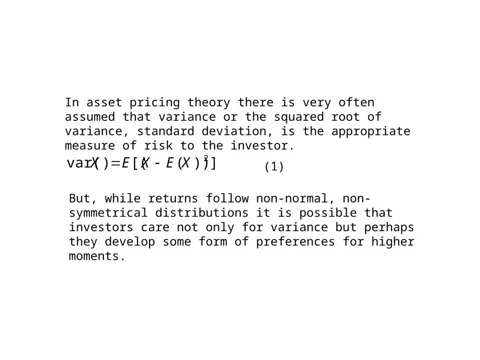
In asset pricing theory there is very often assumed that variance or the squared root of variance, standard deviation, is the appropriate measure of risk to the investor.
But, while returns follow non-normal, non-symmetrical distributions it is possible that investors care not only for variance but perhaps they develop some form of preferences for higher moments.
(1)
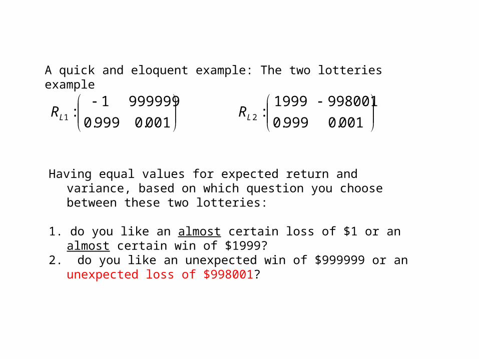
A quick and eloquent example: The two lotteries example
001.0999.0
9999991:1LR
001.0999.0
9980011999:2LR
Having equal values for expected return and variance, based on which question you choose between these two lotteries:
1. do you like an almost certain loss of $1 or an almost certain win of $1999?
2. do you like an unexpected win of $999999 or an unexpected loss of $998001?
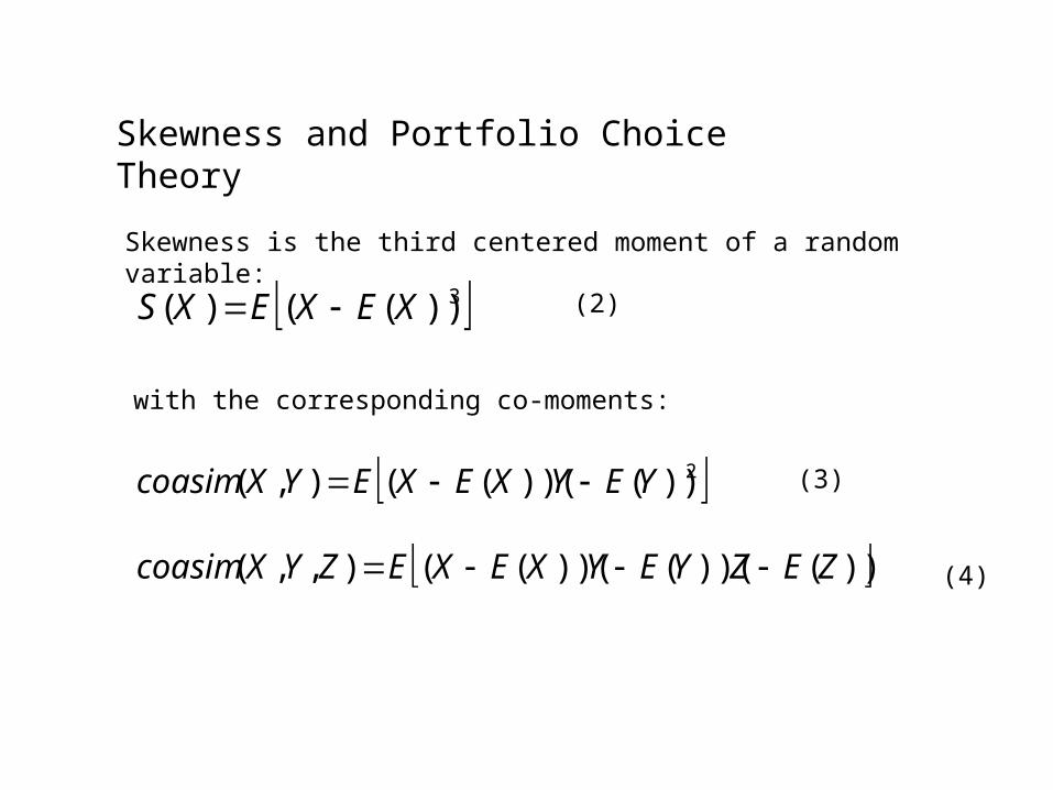
Skewness and Portfolio Choice Theory
Skewness is the third centered moment of a random variable:
3))(()( XEXEXS
with the corresponding co-moments:
2))())(((),( YEYXEXEYXcoasim
))())(())(((),,( ZEZYEYXEXEZYXcoasim
(2)
(3)
(4)

n
i
n
kjij
n
kijkkji
n
i
n
jij
ijjji
n
iiiiiP xxxxxxRS
1 1 11 1
2
1
3 63)(
)(')( xxAxRS P
(5)
(6)A Convenient Notation
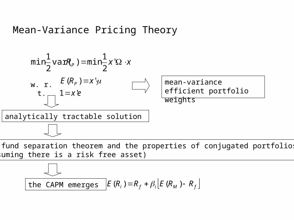
xxRP '2
1min)var(
2
1min
w. r. t.ex
xRE P
'1
')(
analytically tractable solution
two fund separation theorem and the properties of conjugated portfolios (assuming there is a risk free asset)
the CAPM emerges fMifi RRERRE )()(
mean-variance efficient portfolio weights
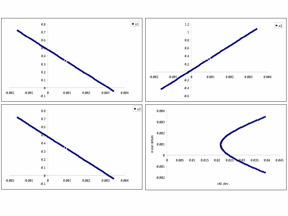
Mean-Variance Pricing Theory
-0.1
0
0.1
0.2
0.3
0.4
0.5
0.6
0.7
0.8
-0.002 -0.001 0 0.001 0.002 0.003 0.004
x1
-0.6
-0.4
-0.2
0
0.2
0.4
0.6
0.8
1
1.2
-0.002 -0.001 0 0.001 0.002 0.003 0.004
x2
-0.1
0
0.1
0.2
0.3
0.4
0.5
0.6
0.7
0.8
-0.002 -0.001 0 0.001 0.002 0.003 0.004
x3
-0.002
-0.001
0
0.001
0.002
0.003
0.004
0 0.005 0.01 0.015 0.02 0.025 0.03 0.035 0.04 0.045
std. dev.
mea
n re
turn
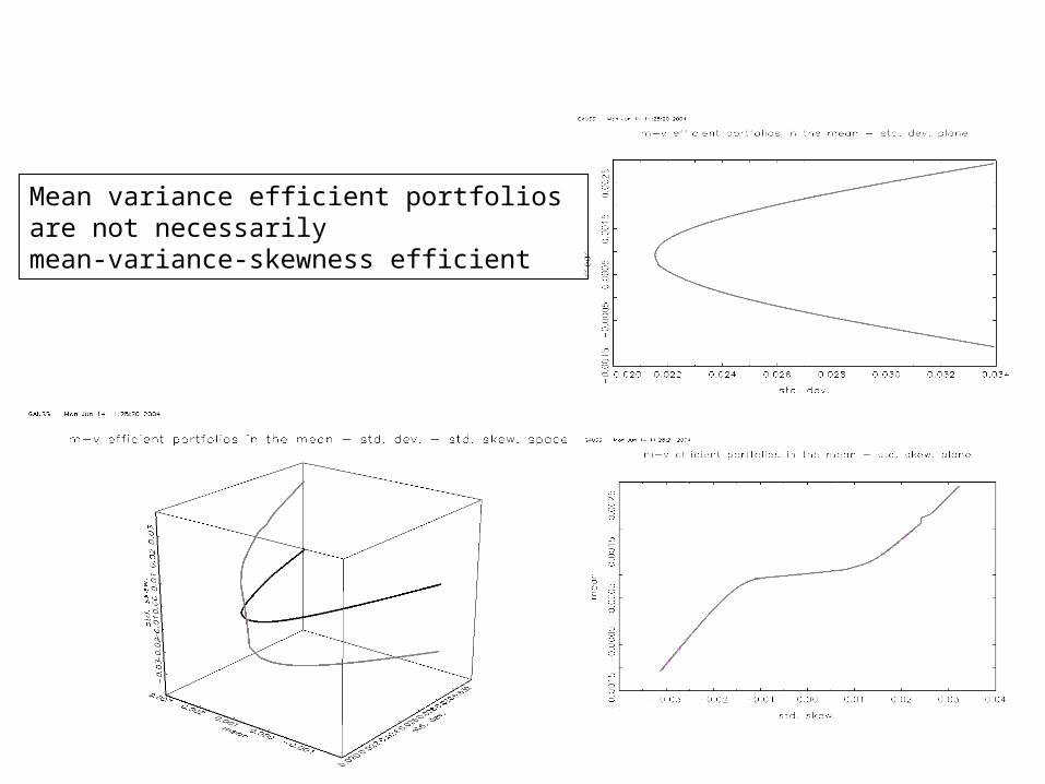
Mean variance efficient portfolios are not necessarilymean-variance-skewness efficient
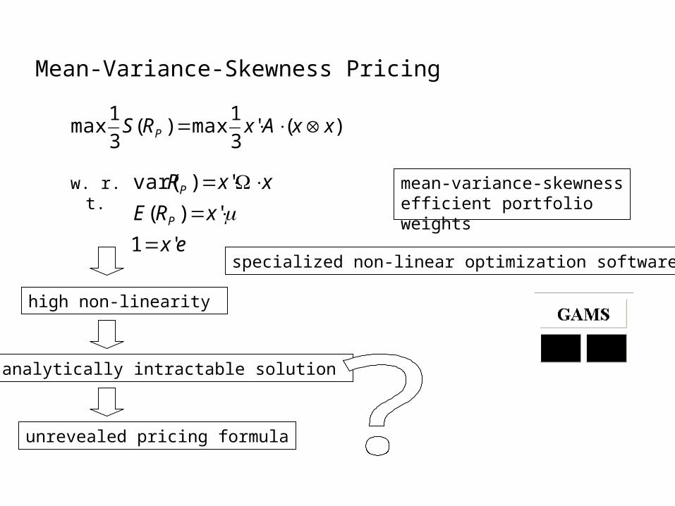
Mean-Variance-Skewness Pricing
)('3
1max)(
3
1max xxAxRS P
w. r. t.
ex
xRE
xxR
P
P
'1
')(
')var(
high non-linearity
analytically intractable solution
unrevealed pricing formula
specialized non-linear optimization software
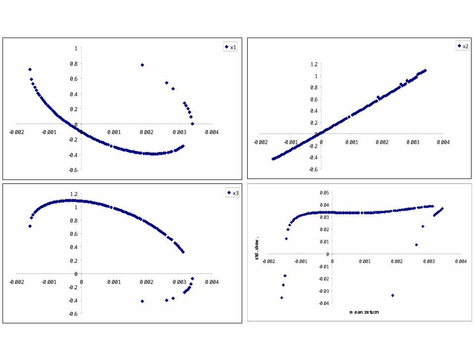
mean-variance-skewness efficient portfolio weights
-0.6
-0.4
-0.2
0
0.2
0.4
0.6
0.8
1
-0.002 -0.001 0 0.001 0.002 0.003 0.004
x1
-0.6
-0.4
-0.2
0
0.2
0.4
0.6
0.8
1
1.2
-0.002 -0.001 0 0.001 0.002 0.003 0.004
x2
-0.6
-0.4
-0.2
0
0.2
0.4
0.6
0.8
1
1.2
-0.002 -0.001 0 0.001 0.002 0.003 0.004
x3
-0.04
-0.03
-0.02
-0.01
0
0.01
0.02
0.03
0.04
0.05
-0.002 -0.001 0 0.001 0.002 0.003 0.004
mean return
std
. ske
w.

An Utility Approach
Assume the investor has a NIARA-class utility function with positive marginal utility and risk aversion for wealth and income (as a stochastic variable).
RrErErWEWUW
rErErWEWUW
rWEWUrWWUE
33
22
))((6
))(('''
))((2
))(("))(())(
(7)
By expanding the utility function in a Taylor series about final (expected)wealth (initial wealth plus period’s income) and taking expectations we get expected utility as a function of the stochastic variable’s moments.

fMMi
Mifi RRE
K
K
KRRE
)(
11
1)(
)(max)](),(),([max)]([max xFxSxVxMFRUE P
s.t. 1' 0 xex
)(')(
')(
)(')(
xxAxxS
xxxV
eRxRxM ff
First order condition: 0x
F
three moment CAPM
(8)
3M
iMMMi m
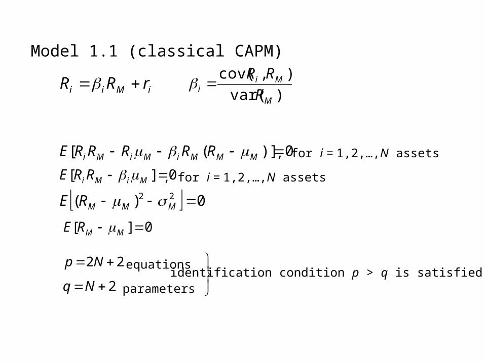
Model 1.1 (classical CAPM)
iMii rRR )var(
),cov(
M
Mii R
RR
0)]([ MMMiMiMi RRRRRE , for i = 1,2,…,N assets
0][ MiMiRRE , for i = 1,2,…,N assets
0)( 22 MMMRE
0][ MMRE
22 Np equations
2Nq parameters identification condition p > q is satisfied

)var(
),cov(
M
Mii q
qr )(
),(~
M
Mii RS
Rrcoasim
ii ~

Model 1.2
iMii qr 2MM Rq
)var(
),cov(
M
Mii q
qr
0)]([ qMMMiqMiMi qqrqrE
, for i = 1,2,…,N assets0][ qMiMiqrE , for i = 1,2,…,N assets
0)( 22 qMqMMqE 0][ qMMqE
22 Np equations
2Nq parameters identification condition p > q is satisfied
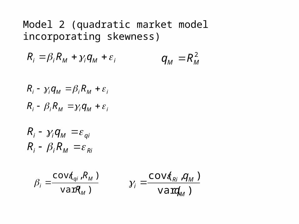
Model 2 (quadratic market model incorporating skewness)
iMiMii qRR 2MM Rq
iMiMii RqR
iMiMii qRR
qiMii qR
RiMii RR
)var(
),cov(
M
Mqii R
R
)var(
),cov(
M
MRii q
q

0 qMiMiiRE for i = 1,2,…,N assets
0)( MMMiMqiMqi RRRE for i = 1,2,…,N assets
0)( qMMMiqMRiMRi qqqE for i = 1,2,…,N assets
0 MMRE 0 qMMqE
23 Np equations
22 Nq parameters identification condition p > q is satisfied
0 1
2121 )(
),...,,(
!
1),...,,(
i
i
kk
n
k k
nn xx
x
xxxf
ixxxf
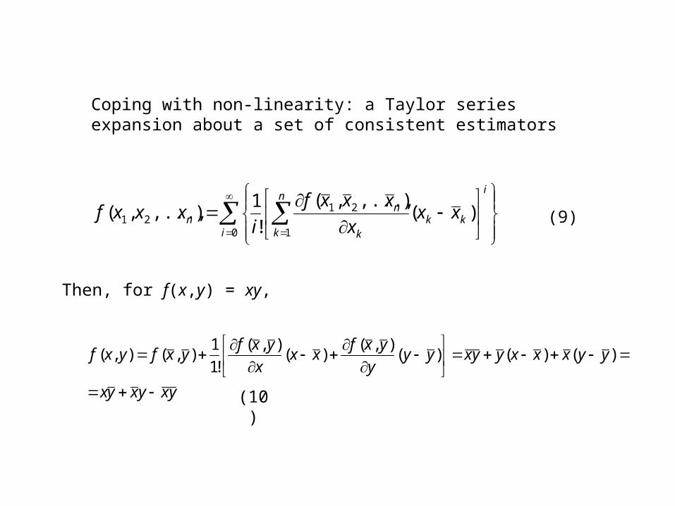
Then, for f(x,y) = xy,
yxyxyx
yyxxxyyxyyy
yxfxx
x
yxfyxfyxf
)()()(
),()(
),(
!1
1),(),(
Coping with non-linearity: a Taylor series expansion about a set of consistent estimators
(9)
(10)
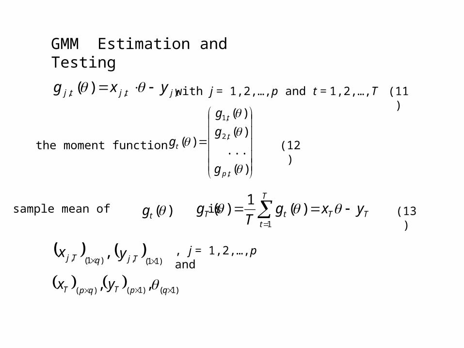
GMM Estimation and Testing
tjtjtj yxg ,,, )( with j = 1,2,…,p and t = 1,2,…,T
)(
...
)(
)(
)(
,
,2
,1
tp
t
t
t
g
g
g
gthe moment function
sample mean of is )(tg TT
T
ttT yxg
Tg
1
)(1
)(
(11)
(12)
(13)
,)1(, qTjx
)11(, Tjy , j = 1,2,…,p and
,)( qpTx ,)1( pTy )1( q

According to Hansen [1982], the GMM estimator minimizes
)()()'()( 1 TT gVTgq
the covariance matrix estimator for the model’s parameters
)'()(1
)(1
t
T
tt gg
TV
TTTT yVxxVx )('))('( 111 estimating the parameter vector
(14)
(15)
(16)
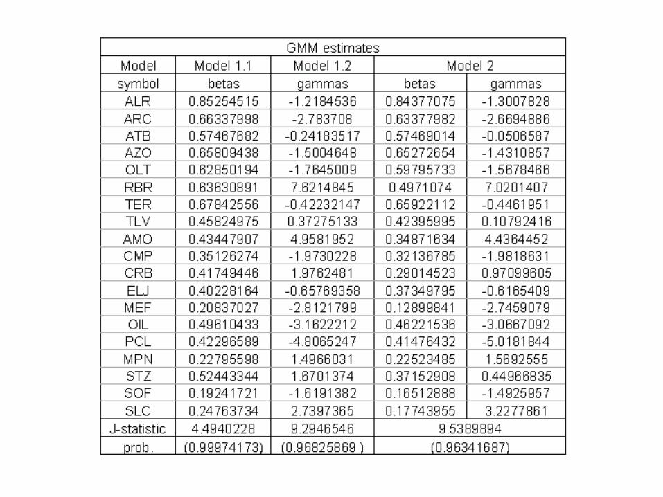
0)]([ tgE:0HThe J-test.
)()ˆ()ˆ()'ˆ( 21 qpgVTgJ dTT
Having p (moment conditions) > q (parameters), then
(17)

Data
The data used for this analysis consists of series of daily returns of nineteen liquid stocks traded at the Bucharest Stock Exchange, on both the first and second tiers, starting from April 17th 1998 to December 19th 2002, giving a total of 1136 observations. These stocks are: Alro, Arctic, Antibiotice, Azomures, Oltchim, Rulmentul, Terapia, Banca Transilvania, Amonil, Compa, Carbid-Fox, Electroaparataj, Mefin, OilTerminal, Policolor, Mopan, Sinteza, Sofert and Silcotub. The BSE is a young market so these stocks were chosen in order to provide a large sample of observations for estimation. The BET-C index was used as a proxy for the market portfolio. For the risk free rate there was used the medium interest rate for deposits on the inter-banking market, BUBID.The whole period was divided in three equal sub-periods in order to check if there are major discrepancies in test statistics across time.
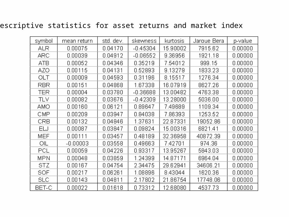
Descriptive statistics for asset returns and market index

The empirical density vs. the normal density for the market index returns
The empirical cumulative distribution function versus the normal cumulative distribution function for the market index

GMM test statistics
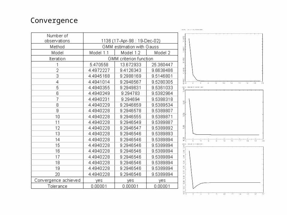
Convergence

betas
0
0.1
0.2
0.3
0.4
0.5
0.6
0.7
0.8
0.9
1 2 3 4 5 6 7 8 9 10 11 12 13 14 15 16 17 18 19
Sample Equivalents
GMM estimates
gammas
-6
-4
-2
0
2
4
6
8
10
12
1 2 3 4 5 6 7 8 9 10 11 12 13 14 15 16 17 18 19
Sample Equivalents
GMM estimates
betas
0
0.1
0.2
0.3
0.4
0.5
0.6
0.7
0.8
0.9
1 2 3 4 5 6 7 8 9 10 11 12 13 14 15 16 17 18 19
Sample Equivalents
GMM estimates
gammas
-6
-4
-2
0
2
4
6
8
10
12
1 2 3 4 5 6 7 8 9 10 11 12 13 14 15 16 17 18 19
Sample Equivalents
GMM estimates
Model 1.1 Model 1.2
Model 2: betas Model 2: gammas

We have briefly illustrated how to deal with multi-moment portfolio analysis by using appropriate conventional notation, specifically designed procedures programmed in Gauss and nlp solvers like MINOS or CONOPT provided by optimization software like GAMS in order to compensate for the intractability of analytical solutions.
In the absence of an analytical solution provided by a non-linear optimization problem and believing that an utility based pricing model is to restrictive in it’s assumptions to be supported by actual data, we test if a quadratic model as the ones suggested by Barone-Adesi, Urga and Gagliardini [2003] or Harvey and Siddique [2000b] is indeed incorporating a measure of systematic skewness. Using the Generalized Method of Moments, and specifically designed procedures implemented with Gauss we find that all the models tested perform well, the test statistic confirming the null hypothesis of orthogonality.
Conclusions