the 8th rmutp international conference on science
TRANSCRIPT

The 8th RMUTP International Conference on
Science, Technology and Innovation for
Sustainable Development: Challenges towards
digital society
Pullman Bangkok King Power, Bangkok,
Thailand, 22-23 June 2017

Asia-Pacific Applied Economics Association Conference Proceedings
The 8th RMUTP International Conference, Bangkok, Thailand, 2017
Editorial Note
Editor-in-Chief: Paresh Kumar Narayan, Alfred Deakin Professor, Deakin University
Series Editor: Seema Narayan, Associate Professor, RMIT University
Asia-Pacific Applied Economics Association (APAEA) conference proceedings publishes high
quality papers selected out of papers presented at APAEA’s conferences. Each APAEA
conference is affiliated with either SCOPUS indexed or social science citation indexed
journals. The APAEA conferences encourage presentation of papers broadly in the fields of
economics and finance that make use of advanced econometric techniques and new datasets to
test economic models and hypotheses related to finance and economics. Common topics of
importance to conference participants are those that test economic models and hypothesis using
new datasets and/or methods, forecasting financial time-series data, financial market
performance, macroeconomic stability issues, panel data models, energy finance, economic
growth and productivity, and econometrics methods including financial econometrics. These
are the types of papers that are ultimately published in the APAEA conference proceedings.
The APAEA conference proceedings follow a single blind review procedure. All papers
submitted to the conference go through a single blind review procedure such that those papers
that are ultimately published in the Proceedings have undergone a review process. The
conference and, therefore, the Proceedings rejection rate stands at 50%. The low quality papers,
which in the view of the conference scientific committee and the Editor of the Proceedings
have low chances of advancing knowledge and contributing to the literature are desk rejected
without sending the papers for a formal review.
All APAEA publications, including the Proceedings, follow the publication ethics and
malpractice statements developed for editors and authors by Wagner & Kleinert (2011). See
https://publicationethics.org/node/11184 for details and full bibliographical information on
Wagner & Kleinert (2011).

Asia-Pacific Applied Economics Association Conference Proceedings
The 8th RMUTP International Conference, Bangkok, Thailand, 2017
TABLE OF CONTENT
1. Intricacies of Competition, Profitability & Stability in Dual Banking Economies. Does
Presence of Islamic Banks Change the Dynamics?
Wajahat Azmi, Mohsin Ali, Shaista Arshad, Syed Aun R. Rizvi
Page 1-19
2. Modelling Market Integration in the Middle East and Africa through the Law of One Price
Vinh Q.T. Dang, Yu (Alan) Yang
Page 20-44
3. Oil Palm, Land Use Change and Community Livelihoods in Indonesia: A Policy Simulation
Analysis
Dennis Mark Onuigbo, Bonar Marulitua Sinagab, Hariantoc
Page 45-61
4. Simultaneous Determinants of Fiscal Policy, Monetary Policy, Income Inequality, Trade,
Domestic Credit to Private Sector and Economic Growth: Case of Emerging Market Economy
Dipyaman Pal and Arpita Ghose
Page 62-89
5. Testing Commodity Futures Market Efficiency under Time-Varying Risk Premiums and
Heteroscedastic Prices
Duminda Kuruppuarachchi, Hai Lin, I. M. Premachandra
Page 90-133
6. Does Energy Consumption Fuel Long-Run Productivity Growth? Panel Evidence from Global
Data with New Policy Insights
Badri Narayan Rath, Vaseem Akram, Debi Prasad Bal, Mantu Kumar Mahalik
Page 134-171
7. Capital-Enhanced Equilibrium Exchange Rate In The Presence Of Structural Breaks: Evidence
from Selected EME’s And Advanced Economies
Prabheesh K.P. and Bhavesh Garg
Page 172-186
8. Is Stock Market Sensitive to Day-to-Day Monetary Operations? Evidence from an Emerging
Economy
Radeef Chundakkadan
Page 187-206
9. US Economic Uncertainty, EU Business Cycles and the Global Financial Crisis
Taufiq Choudhry, Syed S. Hassan, Sarosh Shabi
Page 207-228
10. How Does Microfinance Prosper? An Analysis of ESG Context
Tauhidul Islam Tanin, Mohammad Ashraful Mobin, Adam Ng, Ginanjar Dewandaru
Page 229-264

Asia-Pacific Applied Economics Association Conference Proceedings
The 8th RMUTP International Conference, Bangkok, Thailand, 2017
1
Intricacies of Competition, Profitability & Stability in Dual Banking Economies. Does
Presence of Islamic Banks Change the Dynamics?
Wajahat Azmi*, Mohsin Ali*, Shaista Arshad**, Syed Aun R. Rizvi***
*INCEIF, Kuala Lumpur, Malaysia
**Nottingham University Business School, University of Nottingham Malaysia Campus,
Semenyih, Malaysia
***Suleman Dawood School of Business, Lahore University of Management Sciences
(LUMS), Lahore, Pakistan. Email: [email protected]
Abstract
This paper adds to the debate on the impact of competition and on bank stability and
profitability. The novelty lies in analyzing the impact of studying the nexus of stability and
competition, and performance and competition in dual banking We aim to examine whether
(1) Islamic banks contribute towards overall banking stability, (2) conventional banks benefit
from Islamic banks in a dual banking system and (3) whether the relationship between
competition and stability is heterogeneous across banks in a dual banking system. Our results
show that in general, Islamic banks increases the stability of commercial banking sector and
are inherently more stable themselves but with similar profitability. Furthermore, there is a
homogenous effect of competition on stability and profitability across bank types. To add
robustness to our results, multiple proxies are used for competition, stability and profitability.
A further analysis is conducted on split sample based on size as measured by total assets.
Keywords: Competition, Boone index, Stability, Islamic banks, Dual banking economies
JEL Classification: D40, G21, Z12

Asia-Pacific Applied Economics Association Conference Proceedings
The 8th RMUTP International Conference, Bangkok, Thailand, 2017
2
1. Introduction This paper adds a novel dimension of dual banking systems to the intensely debated topic of
whether competition is good for banking stability and profitability. Researchers remain divided
on its impact; where one group are of the opinion that competition has a positive effect on
stability, known as the competition-stability view (Leroy and Lucotte, 2016; Fiordelisi and
Mare, 2014; Schaeck and Cihák, 2014 and Pawlowska, 2015). The second group argue based
on competition-fragility, as increasing competition leads to greater risk taking and instabilities
prompting banking problems (Keeley, 1990; Jiménez et al., 2013; Weill, 2013; Allen and Gale,
2000 and Hellmann et al. 2000).
The expansion of Islamic banks over the last two decades has further complicated the debate
on bank competition and stability in three major ways. (1) Islamic banks have reported strong
growths globally with 34% of the market share in GCC countries and 13% in ASEAN
countries. With the incessant growth of Islamic banking, the shifting degrees of market power
may bear serious implications for competition and banking stability. (2) In its risk sharing and
interest free nature, Islamic bank’s charter prohibits the inclusion of several toxic assets, raising
the question of whether the impact of competition would have the same effect. (3)
Theoretically, Islamic banks are deemed more stable and resilient, particularly during crisis
periods (Farooq and Zaheer, 2015), opening avenues for healthier economic stability overall.
It can be argued whether diversification between Islamic and conventional banks would benefit
the industry.
Structurally, the presence of Islamic banks in a dual banking system provides a parallel market
for both banks while sharing the same clientele base. Islamic banks provide a channel for
diversification between banks, albeit in a limited capacity. Choi and Kotrozo (2006), Valverde
and Fernandez (2007) found that diversification enhances banks revenue and helps increase
market share, leading to more competitiveness in the industry. Chiorazza’s et al. (2008)
analysis for Italy post shift towards non-interest revenues found a positive relation between
income diversification and risk-adjusted returns. Theoretically, we can apply the same
argument to the interest free nature of Islamic banks, where Molyneux and Yip (2013)
examined the effects of diversification of Islamic banks and found interest-free income to have
a positive influence on banks risk-adjusted performance.
Against this backdrop, the objectives of this study are to analyze whether: (1) Islamic banks
contribute towards overall banking stability, (2) conventional banks benefit from Islamic banks
in a dual banking system and (3) the relationship between competition and stability is
heterogeneous across banks in a dual banking system.
To address our objectives we first delve into measurement of competition, stability and
profitability. Once, we obtain the measures our stability and profitability equations are tested
by employing system GMM methodology. The measurement of our three parameters is divided
into three phases. First, to measure competition, three measures are used: the Boone index as
proposed by Boone (2008), H-statistics and the Herfindahl–Hirschman Index. Second, to
analyze bank stability, we use two alternative measures, Z-score and loan loss provisions to
equity (LLP/E) ratios is used. Third, return on asset and return on equity are used as measures
of profitability.
Our analysis revealed four new results. First, Islamic banks appear more stable across both
stability proxies, which are in line with Beck et al. (2013), who argued these findings based on
the argument that Islamic banks are better capitalized. Second, our findings suggest that the

Asia-Pacific Applied Economics Association Conference Proceedings
The 8th RMUTP International Conference, Bangkok, Thailand, 2017
3
presence of Islamic banks brings banking stability. This is in line with Cihak and Hesse (2007).
Third, Islamic banks outperformed in terms of profitability and stability during the crisis as
compare to conventional banks. This can be owing to Islamic banks restrictions in investing in
toxic assets considered as one of the main reasons for the collapse. Fourth, while diversification
brought stability for both types of banks, it was more effective in the case of Islamic banks.
The results are in line with our expectations as most of the risk management/hedging tools are
not compatible with the Islamic law and the only way to diversify the risk is to venture into
non-intermediation activities.
The current study extends existing literature with three major contributions. First, our findings
lend support to the competition-stability view led by Boyd and De Nicolo (2005) that
competition is associated with more stability. However, in our analysis competition is also
associated with lower profitability. Second, the results are consistent across both type of banks
suggesting that the impact of competition is homogeneous and not contingent on the bank
types. This lends credibility to existing views on competition and banking stability. Third, the
results indicate that the presence of Islamic banks increases the stability of conventional banks.
Indicating that conventional banks engaging in Islamic finance might have benefited from
diversifying their portfolio and thus limiting their exposure to risky assets. Moreover, our
results showed Islamic banks to be more stable as compared to their conventional peers but
with similar profitability. This adds to the emerging literature on the support of Islamic banking
and finance.
To reaffirm the results obtained, the empirical evidence is subjected to multiple robustness
tests. Firstly, we use three different proxies for stability, namely Boone index, H-Statistics and
the Herfindahl–Hirschman Index. The results are consistent across all the three measures of
competition. Secondly, we use two different proxies of stability (Z-score, the ratio of loan loss
provision to equity and profitability (return on assets and the return on equity). Our results
generally conformed despite different measures. Lastly, we split the sample based on size,
measured by total assets. In general, the results are in line with the full ample.
Following the introduction in Section 1, section 2 and 3 explore the data and methodological
construct of our study respectively. Section 4 discusses the empirical results and section 5
provides the conclusion.
2. Data
To achieve our proposed objectives, our sample dataset consists of 398 banks, out of which
106 are Islamic and 292 are conventional. Data is obtained from Bankscope for a period of 9
years from 2005-2014. Selecting countries with dual banking systems, after adjusting for data
availability and consistency issues, leaves us with 15 countries, namely: Bahrain, Bangladesh,
Brunei, Indonesia, Jordan, Kuwait, Lebanon, Malaysia, Pakistan, Qatar, Saudi Arabia, Tunisia,
Turkey, UAE and Yemen.
In order to measure bank performance, both traditional and frontier measures are employed. In
additional to traditional measures, Table 1 provides the descriptive statistics of the Z-score,
Boone Index, HH Index and H-statistics. Overall, the mean of Z-score is 26.63 with the
standard deviation of 28.830. Comparison of Z-scores of Islamic and conventional suggests
that mean Z- scores of Islamic banks are slightly better than conventional banks. Similarly, the
ratio of cost to income suggests that the Islamic banks are more cost efficient. Both banking
systems appear to be capitalized equally. In terms of profitability, Islamic banks fare better
than conventional banks as suggested by their ROA and ROE. Competition measures suggest

Asia-Pacific Applied Economics Association Conference Proceedings
The 8th RMUTP International Conference, Bangkok, Thailand, 2017
4
that Islamic banks are more competitive owing to Islamic banks having a different client base
and there is competition within Islamic banks to attract this pool.
3. Methodology
The methodology used in this study delves into two aspects primarily, firstly the estimation of
the measurements of the competition, stability and profitability and secondly the econometric
modelling for addressing the research questions.
A. Measurement of Competition
In this paper, the main approach to estimate competition is based on the Boone index (2008).
In addition, for robustness tests we rely on Herfindahl–Hirschman Index (HH Index) and H-
Statistics. The reason for relying on Boone index as the main variable is its apparent advantages
over the traditional measures, such as H-statistics, Lerner Index, concentration ratio. In
comparison to H-statistic, Boone index does not impose long-run equilibrium restriction. It
captures the capability of efficient banks to reallocate profits, based on their cost advantage,
from the inefficient ones in the market as highlighted by Schaeck & Cihak (2014). Claessens
and Laeven (2004) had argued that concentration ratio and Herfindahl-Hirschman (HH) index
do not fully capture the competition in banking industry. Even other proxies such as the Panzar
and Rosse (1987) H-Statistic and the Lerner index have been criticized for not being able to
fully capture competition.
The intuition underlying the Boone index has its roots in the efficiency hypothesis, which
argues that performance correlates with efficiency (Demsetz, 1973). Precisely, this hypothesis
maintains that banks with lower cost to income ratio, that is, banks with cost advantages can
gain superior performance and grow at the cost of their less efficient counterparts. Relaxed
entry restrictions establish this effect further.
This indicator, also termed as profit elasticity, is an estimation of percentage loss from an
increased marginal cost of 1 percent. Hence, the intuition is that increase in competition, either
due to products becoming close substitutes or relaxed entry restrictions, will lead to superior
performance of efficient banks as compare to the performance of less efficient banks.
𝜋𝑖𝑡 = 𝛼 + 𝛽𝑙𝑛𝑀𝐶𝑖𝑡 + 𝑒 𝑖𝑡 (1)
In above equation, 𝜋𝑖𝑡 is the profit of the bank i at time t and 𝛽 is the Boone index or profit
elasticity. MC is the marginal cost. As marginal cost is unobservable, we follow Schaeck and
Cihak (2012, 2014) to approximate it using average cost1. Since competition enhances this
negative relationship, the greater the bank competition, the more negative Boone index will be.
Although there are criticisms raised on the traditional measures, in the interest of robustness,
we also used Herfindahl–Hirschman Index (HH Index) and H-Statistics to measure
competition. We estimate HH Index by squaring the market share of each bank and then
summing the squares:
𝐻𝐻 𝐼𝑛𝑑𝑒𝑥 = ∑ (𝑀𝑎𝑟𝑘𝑒𝑡 𝑠ℎ𝑎𝑟𝑒𝑛)2𝑗𝑛=1 (2)
For the estimation of Panzar and Rosse (1987) method of H-Statistics, we rely on following
reduced form equation for each country:
1 Another way of estimating marginal cost is to calculate a translog cost function (Leuvensteijin et al., 2011).

Asia-Pacific Applied Economics Association Conference Proceedings
The 8th RMUTP International Conference, Bangkok, Thailand, 2017
5
𝑙𝑛(𝑇𝑅𝑖𝑡) = 𝛼 + 𝛽1 ln(𝑤𝐿,𝑖𝑡) + 𝛽2 ln(𝑤𝐹,𝑖𝑡) + 𝛽3 ln(𝑤𝐹𝐶,𝑖𝑡) + 𝛽4 ln(𝑌1,𝑖𝑡)
+ 𝛽5 ln(𝑌2,𝑖𝑡) (3)
In the above equation, our dependent variable 𝑇𝑅𝑖𝑡 is total revenue measure as the ratio of total
interest and non-interest revenue to total assets of bank i at time t. Three input prices,𝑤𝐿,𝑖𝑡,
𝑤𝐹,𝑖𝑡 and 𝑤𝐹𝐶,𝑖𝑡 are cost of labor (ratio of personnel expenses to total assets), cost of funds
(ratio of interest expenses to total deposit) and cost of fixes assets (ratio of other operating and
administrative expenses) respectively. Following Gelos and Roldos (2004) and Claessens and
Laeven (2004) and Cihak and Hesse (2010), we also include certain bank level control
variables. In above equation, 𝑌1,𝑖𝑡 and 𝑌2,𝑖𝑡 represent the ratio of equity to total assets and net
loans to total assets, respectively.
B. Measurement of Stability
For measuring stability, we use the Z-score as suggested and used in banking literature (See:
Lepetit et al., 2008; Laeven and Levine, 2009; Cihak and Hesse, 2007, 2010). For robustness
purpose we use the alternative Loan loss provision to equity of bank.
Z-score is estimated as follows:
𝑍 − 𝑠𝑐𝑜𝑟𝑒 =𝑅𝑂𝐴 + 𝐸
𝑇𝐴
𝜎𝑅𝑂𝐴 (4)
where ROA is the return on assets, E/TA is the equity to total assets ratio, and σROA is the
standard deviation of return on assets. Z-score reflects the probability of banks becoming
insolvent. Therefore, higher the Z-score lower the probability of banks becoming insolvent.
After obtaining the estimates of competition and stability measures, we run the following
specification to test our stability:
𝑆𝑡𝑎𝑏𝑖𝑙𝑖𝑡𝑦𝑖,𝑗,𝑡 =
𝑓(𝑆𝑡𝑎𝑏𝑖𝑙𝑖𝑡𝑦𝑖,𝑗,𝑡−1 𝐶𝑜𝑚𝑝𝑒𝑡𝑖𝑡𝑖𝑜𝑛𝑗,𝑡, 𝐺𝐷𝑃 𝑝𝑒𝑟 𝑐𝑎𝑝𝑖𝑡𝑎𝑗,𝑡, 𝐼𝑠𝑙𝑎𝑚𝑖𝑐 𝑏𝑎𝑛𝑘𝑖𝑛𝑔 𝑠ℎ𝑎𝑟𝑒𝑗𝑡, 𝑍𝑖,𝑗,𝑡, 𝐼𝑠𝑙𝑎𝑚𝑖𝑐𝑖,𝑗
(5)
We use two proxies for our stability measure. In the above equation, 𝑆𝑡𝑎𝑏𝑖𝑙𝑖𝑡𝑦𝑖,𝑗,𝑡 refers to the
Z-score and the ratio of Loan loss provision to equity of bank i at time t in a country.
𝐶𝑜𝑚𝑝𝑒𝑡𝑖𝑡𝑖𝑜𝑛𝑖,𝑗 refers to our estimated HH Index, H-Statistics and Boone index. Islamic
banking share refers to the share of Islamic banks in terms of assets in the banking industry. Z
refers to the control variables such as cost to income ratio, total assets, diversification index,
𝐼𝑠𝑙𝑎𝑚𝑖𝑐𝑖,𝑗 is a dummy variable that takes the value of 1 in case bank i is an Islamic bank2.
C. Measurement of Profitability
In order to explore the objective of profitability we use two alternative measures namely ROA
and ROE. The control variables in the above two equations are the same. A dummy variable is
used for crisis period interacting with the Islamic bank dummy to investigate the impact of
crisis on stability and performance of Islamic banks. 𝑃𝑟𝑜𝑓𝑖𝑡𝑎𝑏𝑖𝑙𝑖𝑡𝑦𝑖,𝑗,𝑡 =
𝑓(𝑃𝑟𝑜𝑓𝑖𝑡𝑎𝑏𝑖𝑙𝑖𝑡𝑦𝑖,𝑗,𝑡−1 , 𝐶𝑜𝑚𝑝𝑒𝑡𝑖𝑡𝑖𝑜𝑛𝑗,𝑡 , 𝐺𝐷𝑃 𝑝𝑒𝑟 𝑐𝑎𝑝𝑖𝑡𝑎𝑗,𝑡, 𝐼𝑠𝑙𝑎𝑚𝑖𝑐 𝑏𝑎𝑛𝑘𝑖𝑛𝑔 𝑠ℎ𝑎𝑟𝑒𝑗𝑡 , 𝑍𝑖,𝑗,𝑡 , 𝐼𝑠𝑙𝑎𝑚𝑖𝑐𝑖,𝑗)
(6)
2 For set of control variables, we refer to Angkinand and Wihlborg (2010), Jeon et al. (2011) and Lee and Hsieh
(2013, 2014).

Asia-Pacific Applied Economics Association Conference Proceedings
The 8th RMUTP International Conference, Bangkok, Thailand, 2017
6
Table 2 summarizes the alternative proxies that this study utilizes to undertake a robust
analysis.
D. Econometric Method
To estimate the above two equations, we use dynamic panel data approach, following the works
of Lee and Hsieh (2014), Fu et al., (2014) and Jimenez et al., (2013). We employ panel GMM
methodology for the following reasons. (1) It controls for endogeniety concerns when there is
a reverse causality from stability to competition and other independent variables3. (2) There is
a possibility that some of the unobserved bank characteristics are correlated with our dependent
variables4. (3) Using panel GMM is more suited to handle minor series with large cross-
sections, as is our case where the dataset spans for 10 years.
To decide between first-difference and system GMM, we rely on the coefficient of lagged
dependent variable and the random walk properties of the variables5. Moreover, system GMM
is advisable in case of unbalanced panel as the first-difference GMM further magnifies this gap
(Roodman, 2009). Based on the autoregressive parameter, we prefer system GMM as the
necessary condition for using system GMM is high persistence in series6.
4. Empirical Results
The empirical results are presented in Table 3 and 4. Table 3 presents the results for the Stability
and competition nexus (See Eq 5 above) while Table 4 presents the GMM estimations for the
profitability and competition nexus (See Eq 6 above).
As discussed earlier, we have used two alternative measures for bank stability, namely Z-Score
and Loan Loss Provisions to equity. In Table 3, Panel A presents the findings with Z -score as
measure of Stability while Panel B uses Loan loss provision to equity (LLP/E) as stability
measure. While the (1), (2) and (3) in each panel represents the three alternative measures of
competition; H-Statistics, HH Index, and Boone Index respectively.
A. Stability and Competition
The following discussion first delves into the stability and competition nexus and then follows
it with the profitability competition while trying to explain the interlinkages of the results.
The Table 3-Panel A results where stability is measured by Z-scores the results suggest a
difference between Islamic banks and conventional banks since the Islamic banking dummy is
significant and positive.
[Insert Table 3 around here]
It suggests that the Islamic banks are more stable as compare to conventional banks. This may
be owing to the prohibitive law in Islamic banking, which prohibits the investment in derivative
and exotic instruments like Credit Default Swaps and other derivative instruments, which had
major contribution to the recent financial meltdown of 2007. The findings are further
reaffirmed when we use the alternative stability measure of Loan loss provision to equity.
3 See Lee and Hsieh (2014). 4 For instance, Jimenez et al., (2013) note that NPL ratios (dependent variable) in their case may be correlated
with the unobserved bank characteristics such as the risk appetite of bank managers and/or shareholders. 5 System is superior to first-difference GMM in presence of random walk variables and the autoregressive
coefficient that is close to unity (Roodman, 2009 and Sarafidis et al., 2009). 6 For instance, Roodman (2009) suggests that the autoregressive parameter of 0.8 and above is a good indication
of high persistence and in that case system GMM produce superior results than the first-differenced GMM.

Asia-Pacific Applied Economics Association Conference Proceedings
The 8th RMUTP International Conference, Bangkok, Thailand, 2017
7
The control variables used primarily concur to expectations and earlier literature in terms of
their relationship signs. Cost to income ratio and loan to asset ratio has a significant negative
relationship as expected in all the models. Further, one of our focal variable, diversification
index suggest that the diversification has positive and significant effect on the stability. The
findings are similar for the interaction of Islamic dummy and diversification index. These
findings suggest that income source diversity brings stability to the banking system. It can be
further be cautiously deduced that a diversifying away from traditional lending activities to
other areas such as trading and fee based income would make the overall system more stable.
Specific to Islamic banks the interaction term is significantly positive, which suggest that
diversification brings more benefit to Islamic banks. This conclusion can be explained by the
nature of Islamic banking activities, which are restricted by Shariah law in indulging in
derivatives for hedging purposes. This exposes the balance sheet of Islamic banks to multiple
risks, which can only be minimized through diversification to non-intermediation income.
These results hold with the alternative measure of stability (Loan loss provision to equity).
Recently Ibrahim and Rizvi (2017) has argued on the banks size matters for Islamic banks
performance. Our findings related to the size (measured by assets) provides evidence for a
negative relationship between size and stability and competition of the banks. The earlier works
of Cihak and Hesse (2007) can explain the findings, who had suggested towards increasing
riskiness of asset nature of banks as size grows.
An extension to the earlier findings is nested in the impact of Islamic Banking share in the
banking industry. With both proxys of stability (Z-score and Loan loss provision to equity), the
impact of Islamic bank share is positive and significant and suggesting that the presence of
Islamic banks adds to the banking stability in the dual system. It should be noted that the results
point to the average effect based on the presence of Islamic and the conventional banks7.
Furthermore, our results also suggest that increase in Islamic banks adds to the stability of
conventional banks.
B. Profitability and Competition
In terms of using different proxies for profitability, the results suggest that profitability (ROA
and ROE) of Islamic banks is higher than the conventional banks only in the model where
Boone index (Table 4 – Panel B (3)) is used. Our finding remains inconclusive towards
suggesting a higher profitability of Islamic banks as compared to their conventional
counterparts in contrast to poular literature which suggests that Islamic banks are more
profitable as compare to conventional banks (See: Samad, 1999; Samad & Hassan, 1999; Iqbal,
2001; Hassoune, 2002). However, our results reaffirm the findings of Turk-Ariss (2010) whose
analysis suggested that the Islamic banking operations do not necessarily bring more rewards
as compare to their conventional peers.
[Insert Table 4 around here]
In terms of the impact of diversification on profitability our results suggest it to be insignificant
for both Islamic and conventional banks. Similar insignificant results are seen for the
interaction term between Islamic banks dummy and diversification coefficient. Earlier the
study had highlighted that a higher presence of Islamic banks adds to the stability of the system.
But in terms of impact of performance there is no significant relationship suggesting that
presence of Islamic banks in a dual system does not contribute towards increasing profitability
of the banks.
7 See, Cihak and Hesse (2007).

Asia-Pacific Applied Economics Association Conference Proceedings
The 8th RMUTP International Conference, Bangkok, Thailand, 2017
8
While our finding suggest that higher competition is associated with higher stability (Table 3)
but it results in lower profitability (Table 4). These results are conform to the competition-
stability paradigm. Similarly, the results are consistent with the profitability measures as the
competition tends to decrease the profit whereas higher concentration is associated with more
profitability. We can cautiously infer that our results suggest that venturing into a market with
low competition or high concentration could be rewarding for the banks. In case of Islamic
banks, competition measures have different impact on stability (Table 3) and profitability
(Table 4). However, the difference is negligible suggesting there are same incentives for
Islamic banks to enter in the market where the concentration is high or competition is low.
Taking a cue from literature earlier cited about crisis and banking, we investigate the impact of
crisis on our sample, and results suggest that crisis had a negative impact on stability and the
profitability of conventional banks. However, the Islamic banks dummy points towards Islamic
banks tended to perform better as compared to their conventional counterparts.
C. Split Sample Robustness Check
To further check for reliability of our findings, we split the sample based on bank size. The
results are presented in Table 5 and 6 for large banks and in Table 7 and 8 for small banks. We
classify small and large banks following the work of Cihak and Hesse (2010) who suggest that
banks with assets more than USD 1 billion are categorized as large banks.
[Insert Table 5 and 6 around here]
The findings of competition measure in the split sample generally conform to our earlier results.
The Islamic banking dummy is significant and positive in case of small banks in terms of both
stability and profitability (Table 7 and the Table8) while in large banks case (Table 5 and the
Table 6), it is insignificant for both stability profitability. This leads us to conclude that smaller
Islamic banks are more stable and more profitable in comparison to smaller conventional
banks. However, in case of large banks, both the conventional and Islamic banks are similar in
terms of stability and the profitability.
[Insert Table 7 and 8 around here]
On the other hand, the diversification results provide interesting insights as diversification is
significant only for the smaller banks (Table 7) whereas it is insignificant for the case of large
banks (Table 5). The insignificance of the Islamic bank dummy for large banks may suggest
that once the Islamic banks become bigger, it does not benefit from the diversification. Overall,
our results suggest that the diversification is only favorable to small banks, be it Islamic or
conventional. While the impact of diversification on the profitability (Table 6 and the Table 8)
remained similar to the earlier findings suggesting diversifying into non-intermediation
activities does not have any effect on banks.
The impact of Islamic Banking share on their counterparts for the split sample confirms our
earlier results, suggesting that the increase in Islamic banking share on average, irrespective of
the whether the bank is big or small, adds to the overall stability of conventional banks. While
higher presence of Islamic banks does not affect the profitability of the other banks in the

Asia-Pacific Applied Economics Association Conference Proceedings
The 8th RMUTP International Conference, Bangkok, Thailand, 2017
9
system. Also, the higher presence of Islamic banks does not influence the profitability of the
conventional banks8.
5. Conclusion
The importance of finance for growth has led the researchers to explore the determinants of
sound banking system. One such strand of the literature explores the impact of competition on
banking stability and profitability. We provide robust results on this as we have utilized three
different proxies of competition and two proxies for stability and profitability measures. Our
results summarizes as follows. First, the presence of Islamic banks increases the stability of
conventional banks. Second, Islamic banks are more stable as compare to their conventional
peers but with similar profitability. This finding is in sharp contradiction with the theoretical
standing of Islamic banks being more profitable. This may be due to the significant divergence
of Islamic banks from the theory as it is supposed to operate on the risk sharing arrangement.
Third, competition has similar effects on stability and profitability on both the banks. Fourth,
Islamic banks did better in terms of profitability during the crisis as compare to conventional
banks. It also suggests that the Islamic banks were more stable during the crisis period.
Our results have several policy implications for countries aspiring to open avenues for Islamic
banking in their countries. Our findings legitimize the economic value of Islamic banks
whereby, it adds to the overall banking stability. Moreover, the presence of Islamic bank can
attract customers based on religious needs without compromising on the stability of the banking
industry.
8 The sample was also split based on the mean deposit and the results are consistent with those reported in Table
5 to 7. For brevity, the results are not reported (available on request).

Asia-Pacific Applied Economics Association Conference Proceedings
The 8th RMUTP International Conference, Bangkok, Thailand, 2017
10
References
Allen, F., & Gale, D. (2000). Comparing Financial Systems. MIT Press, Cambridge,
Massachussetts.
Beck, T. & Levine, R., (2004). Stock markets, banks, and growth. Journal of Banking and
Finance, 28 (3), pp. 423–442.
Beck, T., Demirgüç-Kunt, A., & Merrouche, O. (2013). Islamic vs. conventional banking:
Business model, efficiency and stability. Journal of Banking and Finance, 37, pp. 433–447.
Beck, T., Levine, R., & Loayza, N., (2000). Finance and the sources of growth. Journal of
Financial Economics, 58 (1–2), pp. 261–300.
Berger, A.N., Klapper, L.F. & Turk-Ariss, R. (2009). Bank competition and financial
stability. Journal of Financial Services Research, 35, pp. 99–118.
Boone, J., (2008). A new way to measure competition. Economic Journal, 118, pp. 1245-
1261
Boyd, J.H., De Nicolo, G. & Jalal, A. (2006). Bank Risk-taking and Competition Revisited.
IMF Working Paper, WP/06/297.
Bresnahan, T.F., (1989). Empirical studies of industries with market power. in R.
Schmalensee and R. Willig (eds.) Handbook of Industrial Organization, Vol. 2, Amsterdam:
Elsevier Science.
Chiorazza, V., Milani, C. & Salvini, F.J. (2008). Journal of Financial Services Research,
33(3), pp.181-203.
Choi, S. & Kotrozo, J. (2006). Diversification, Bank risk and Performance: A Cross
Country Comparison. Rensselaer Polytechnic Institute, mimeo, October 2006.
Cihak, M., & Hesse, H., (2010). Islamic banks and financial stability: an empirical analysis.
Journal of Financial Services Research, 38, 95–113.
Cihak, M., Hesse, H. (2007). Cooperative banks and financial stability. IMF Working Paper
WP/07/2.
Claessens, S., & Laeven, L. (2004). What drives bank competition? Some international
evidence. Journal of Money, Credit and Banking, 36, 563−583.
Demsetz, H. (1973). Industry Structure, Market Rivalry, and Public Policy. Journal of Law
and Economics, 16(1), pp. 1-9.
Farooq, M. and Zaheer, S. (2015). Are Islamic Banks More Resilient During Financial
Panics? Pacific Economic Review, 20(1), pp. 101-124.
Fiordelisi, F., & Mare, D. S. (2014). Competition and financial stability in European
cooperative banks. Journal of International Money and Finance, 45, pp. 1-16.
Hassan, M. K., & Bashir, A. H. M. (2003). Determinants of Islamic banking profitability.
International seminar on Islamic wealth creation (pp. 7−9). UK: University of Durham, July.
Hassoune, A. (2002). Islamic banks’ profitability in an interest rate cycle. International
Journal of Islamic Financial Services, 4, pp.1-13.
Hellmann, T.F., Murdock, K.C., & Stiglitz, J.E. (2000). Liberalization, moral hazard in
banking, and prudential regulation: are capital requirements enough? American Economic
Review, 90, pp.147–165.
Ibrahim, M., Rizvi, S.A.R. (2017). Do we need bigger Islamic banks? An assessment of
bank stability. Journal of Multinational Financial Management, 40, pp.77–91
Iqbal, M. (2001). Islamic and Conventional Banking in the Nineties: A Comparative Study.
Islamic Economic Studies, 8 (2), pp. 1-28.
Iwata, G. (1974). Measurement of Conjectural Variations in Oligopoly. Econometrica,
42(5), pp. 947-966.
Jalil, A., Feridun, M., & Ma, Y. (2010). Finance-growth nexus in China revisited new
evidence from principal components and ARDL bounds tests. International Review of
Economics and Finance, 19 (2), pp. 189–195.

Asia-Pacific Applied Economics Association Conference Proceedings
The 8th RMUTP International Conference, Bangkok, Thailand, 2017
11
Jiménez, G., Lopez, J. A., & Saurina, J. (2013). How does competition affect bank risk-
taking? Journal of Financial Stability, 9(2), pp.185-195.
Keeley, M. (1990). Deposit insurance, risk and market power in banking. American
Economic Review, 80, pp. 1183-1200.
Kendall, J. (2012). Local financial development and growth. Journal of Banking and
Finance 36 (5), pp. 1548–1562.
Laeven, L. & Levine, R. (2009). Bank Governance, Regulation and Risk Taking. Journal
of Financial Economics, 93, pp. 259-275.
Lepetit, L., Nys, E., Rous, P. & Tarazi A. (2008). Bank Income Structure and Risk: An
Empirical Analysis of European Banks. Journal of Banking and Finance, 32, pp. 1452-167.
Leroy, A. and Lucotte, Y. (2016). Structural and Cyclical Determinants of Bank Interest-
Rate Pass-Through in the Eurozone. Comparative Economic Studies, 58(2), pp. 196-225.
Leuvensteijin, M.V., Bikker, J., Rixtel, A.V., & Sorensen, C.K. (2011). A new approach to
measuring competition in the loan markets of the Euro area. Applied Economics, 43, pp. 3155–
3167.
Molyneux, P. & Yip, J. (2013). Income diversification and performance of Islamic banks.
Journal of Financial Management, Markets and Institutions, 1(1), pp. 47-66.
Panzar, J. C., & Rosse, J. N. (1987). Testing for ‘monopoly’ equilibrium. Journal of
Industrial Economics, 35, pp. 443−456.
Pawłowska, M. (2015). On Competition in the Banking Sector in Poland and Europe before
and During the Crisis. Bank–CASE Seminar Proceedings No. 134/2014
Samad, A. (1999). Relative performance of conventional banking vis-à-vis Islamic bank in
Malaysia. IIUM Journal of Economics and Management, 7, pp. 1−25.
Samad, A., & Hassan, M. K. (1999). The performance of Malaysian Islamic bank during
1984–1997: An exploratory study. International Journal of Islamic Financial Services, 1, pp.
1−14.
Schaeck, K. & Cihák, M. (2014). Competition, efficiency, and stability in
banking. Financial Management, 43(1), pp. 215-241.
Schaeck, K., & Cihak, M. (2008). How does competition affect efficiency and soundness in
banking? New empirical evidence. European Central Bank Working Paper No. 232.
Schaeck, K., & Cihak, M. (2012). Banking competition and capital ratios. European
Financial Management, 18(5), pp. 836-866.
Schaeck, K., Cihák, M., & Wolfe, S. (2009). Are competitive banking systems more stable?
Journal of Money, Credit, and Banking, 41, pp. 711-734.
Tabak, B.M., Fazio, D.M., & Cajueiro, D.O. (2012). The relationship between banking
market competition and risk-taking: do size and capitalization matter? Journal of Banking and
Finance, 36, pp. 3366–3381.
Turk-Ariss, R. (2010). Competitive conditions in Islamic and conventional banking: a
global perspective. Review of Financial Economics, 19, pp. 101–108.
Valverde, S.C & Fernandez, F.R. (2007). Do cross-country differences in bank efficiency
support a policy of “national champions”? Journal of Banking and Finance, 31(7), pp.2173-
2188.
Vives, X. (2008). Innovation and competitive pressure. Journal of Industrial Economics,
Vol. 56, pp. 419-469.
Weill, L. (2013). Bank Competition in the EU: How has it evolved? Journal of
International Financial Market, Institutions and Money, 26(C), pp. 100-112.
Yeyati, E. L. & Micco, A., (2007). Concentration and foreign penetration in Latin
American banking sectors: Impact on competition and risk. Journal of Banking &
Finance, 31(6), pp. 1633-1647.

Asia-Pacific Applied Economics Association Conference Proceedings
The 8th RMUTP International Conference, Bangkok, Thailand, 2017
12
Table 1: Descriptive Statistics of Sample Banks
This table provides descriptive statistics for all banks in our sample. Panel A provides statistics
on all 398 banks, while Panel B shows only Islamic banks and Panel C provides information
on conventional banks. Z-score, Boone Index, HH Index, H-statistic, Diversification Index are
calculated by the authors. Remainder are obtained from Bank scope.
Panel A: Full Sample
Variable Obs Mean Std. Dev. Min Max
Z-score* 3321 26.635 28.831 -12.735 512.708
Cost-income 3582 0.509 0.569 0.110 9.500
Loan/Total Asset 3214 0.457 0.257 0.188 1.091
Equity/Total Asset 3582 0.142 0.169 -0.959 1.506
ROA 3215 0.011 0.049 -1.303 0.383
ROE 3214 0.113 0.390 -9.461 9.419
Boone Index* 3582 -0.135 9.661 -3.851 2.383
Total deposit 3582 5430.200 11062.670 2301.800 96161.200
Loan loss provision/Equity (LLP/E) 3213 0.053 0.342 -9.031 8.782
Loan loss provisions 3582 39.727 108.841 -183.942 1533.640
Loans 3582 3643.863 8209.263 2162.700 85360.400
HH Index* 3582 1201.321 656.148 517.608 5172.245
H-Statistic* 3582 0.191 0.197 -0.077 0.631
Diversification index* 3197 -0.298 15.330 -308.013 516.824
Panel B: Islamic banks
Variable Obs Mean Std. Dev. Min Max
Z-score* 890 28.294 27.817 -5.380 492.926
Cost-income 954 0.472 0.423 0.110 8.415
Loan/Total Asset 853 0.487 0.275 0.214.6 1.091
Equity/Total Asset 954 0.142 0.185 -0.959 0.999
ROA 853 0.012 0.048 -0.697 0.322
ROE 853 0.145 0.477 -2.599 9.419
Boone Index* 954 -0.142 5.688 -3.851 2.383
Total deposit 954 3498.312 7500.473 2301.800 59767.500
Loan loss provision/Equity (LLP/E) 853 0.059 0.368 -9.031 3.474
Loan loss provisions 954 28.394 77.174 -48.995 876.332
Loans 954 2424.205 5421.046 2162.700 51809.600
HH Index* 954 1362.302 724.768 517.608 5172.245
H-Statistic* 954 0.220 0.178 -0.077 0.631
Diversification index* 847 -0.212 9.366 -111.790 157.500
Panel C: Conventional banks
Variable Obs Mean Std. Dev. Min Max
Z-score* 2431 25.835 28.379 -12.735 512.708
Cost-income 2628 0.523 0.613 0.417 9.500
Loan/Total Asset 2361 0.446 0.249 0.188 0.927
Equity/Total Asset 2628 0.141 0.163 -0.920 1.506
ROA 2362 0.010 0.049 -1.303 0.383
ROE 2361 0.101 0.353 -9.461 4.741
Boone Index* 2628 -0.132 0.651 -3.851 2.383
Total deposit 2628 6131.502 12023.740 2301.800 96161.200
Loan loss provision/Equity (LLP/E) 2360 0.051 0.332 -4.729 8.782
Loan loss provisions 2628 43.841 118.001 -183.942 1533.640
Loans 2628 4086.616 8970.406 2162.700 85360.400
HH Index* 2628 1142.883 619.266 517.608 5172.245
H-Statistic* 2628 0.180 0.202 -0.077 0.631
Diversification index* 2350 -0.330 16.975 -308.013 516.824

Asia-Pacific Applied Economics Association Conference Proceedings
The 8th RMUTP International Conference, Bangkok, Thailand, 2017
13
Table 2: Summary of Alternative Proxies Used
This table summarizes the different proxies that are used as robustness measures for the three
critical variables under discussion in this research.
Variable Proxies Used
Competition Boone Index H-Statistics HH Index
Stability Z-Score Loan Loss Provision to Equity
Profitability ROA ROE

Asia-Pacific Applied Economics Association Conference Proceedings
The 8th RMUTP International Conference, Bangkok, Thailand, 2017
14
Table 3: System GMM - Stability and Competition
This table presents the GMM estimations for the Stability and competition nexus for the
Equation 5 as presented below.
𝑆𝑡𝑎𝑏𝑖𝑙𝑖𝑡𝑦𝑖,𝑗,𝑡
= 𝑓(𝑆𝑡𝑎𝑏𝑖𝑙𝑖𝑡𝑦𝑖,𝑗,𝑡−1𝐶𝑜𝑚𝑝𝑒𝑡𝑖𝑡𝑖𝑜𝑛𝑗,𝑡 , 𝐺𝐷𝑃 𝑝𝑒𝑟 𝑐𝑎𝑝𝑖𝑡𝑎𝑗,𝑡, 𝐼𝑠𝑙𝑎𝑚𝑖𝑐 𝑏𝑎𝑛𝑘𝑖𝑛𝑔 𝑠ℎ𝑎𝑟𝑒𝑗𝑡 , 𝑍𝑖,𝑗,𝑡 , 𝐼𝑠𝑙𝑎𝑚𝑖𝑐𝑖,𝑗
Panel A presents the findings with Z -score as measure of Stability while Panel B uses Loan
loss provision to equity (LLP/E) as stability measure. While the (1), (2) and (3) in each panel
represents the three alternative measures of competition; H-Statistics, HH Index, and Boone
Index respectively. The superscripts ***, **, and * denote significance at the 1%, 5%, and 10%
levels, respectively
Panel A: Z Score Panel B: LLP/E
1 2 3 1 2 3
H-
Statistics
HH Index Boone
Index
H-
Statistics
HH Index Boone
Index Z Score(-1)
0.892 0.813 0.914
(0.000)*** (0.000)**
*
(0.000)***
LLP/E(-1) 0.792 0.924 0.890
(0.002)*** (0.002)**
*
(0.000)***
Cost to Income
Ratio
-1.044 -1.083 -1.032 0.016 0.015 0.001
(0.011)** (0.008)**
*
(0.012)** (0.008)*** (0.071)** (0.013)**
Loan to Total Asset -3.493 -3.416 -3.499 0.037 0.035 0.037
(0.002)*** (0.002)**
*
(0.001)*** (0.000)*** (0.000)**
*
(0.000)***
Size -0.003 0.024 -0.003 0.006 0.004 0.091
(0.038)** -0.481 -0.421 (0.027)** (0.019)** (0.100)*
Diversification
Index
0.027 0.084 0.076 -0.034 -0.004 -0. 0308
(0.042)** (0.038)** (0.012)** (0.001)*** (0.000)**
*
(0.028)**
Diversification
Index*Islamic
0.002 0.002 0.002 -0.004 -0.002 -0.001
(0.071)* (0.097)* (0.083)* (0.097)* (0.012)** -0.675
Islamic Banking
(IB) Share
2.850 2.640 2.060 -0.021 -0.025 -0.030
(0.000)*** (0.000)**
*
(0.000)*** (0.000)*** (0.000)**
*
(0.000)***
IB Share*CB
Dummy
-1.080 1.930 0.082 -0.091 -0.322 -0.002
-0.101 (0.10)* (0.008)*** (0.083)* (0.091)* -0.173
Islamic 1.300 1.510 1.310 -0.029 -0.026 -0.033
(0.073)* (0.084)* (0.012)** -0.127 -0.713 (0.014)**
GDP per capita 0.008 0.003 0.003 -0.002 -0.019 -0.002
(0.000)*** (0.000)**
*
(0.000)*** (0.000)*** (0.000)**
*
(0.000)***
Competition 1.080 -0.002 1.170 -0.005 0.007 -0.011
(0.096)* (0.065)* (0.019)** (0.028)** (0.013)** (0.025)**
Competition*Islami
c
0.637 -0.001 1.790 -0.017 0.024 -0.013
-0.957 (0.051)* (0.062)** -0.661 (0.067)* (0.084)*
Islamic*Crisis 2.460 2.590 2.350 -0.074 -0.074 -0.073
(0.017)** (0.013)** (0.024)** (0.004)** -0.606 (0.042)**
Crisis -0.292 -0.355 -0.397 0.022 0.022 0.022
(0.098)* -0.121 (0.074)* -0.580 (0.049)** (0.091)*
Constant 24.840 21.890 24.770 0.023 0.036 0.025
(0.000)*** (0.000)**
*
(0.000)*** (0.000)*** (0.000)**
*
(0.000)***
Sargan p-values 0.560 0.420 0.570 0.680 0.610 0.710
AR(1)-p values 0.089 0.092 0.047 0.082 0.071 0.162
AR(2)-p values 0.415 0.588 0.018 0.125 0.089 0.263

Asia-Pacific Applied Economics Association Conference Proceedings
The 8th RMUTP International Conference, Bangkok, Thailand, 2017
15
Table 4: System GMM - Performance and Competition
This table presents the GMM estimations for the profitability and competition nexus for the
Equation 6 as presented below.
𝑃𝑟𝑜𝑓𝑖𝑡𝑎𝑏𝑖𝑙𝑖𝑡𝑦𝑖,𝑗,𝑡
= 𝑓(𝑃𝑟𝑜𝑓𝑖𝑡𝑎𝑏𝑖𝑙𝑖𝑡𝑦𝑖,𝑗,𝑡−1 , 𝐶𝑜𝑚𝑝𝑒𝑡𝑖𝑡𝑖𝑜𝑛𝑗,𝑡 , 𝐺𝐷𝑃 𝑝𝑒𝑟 𝑐𝑎𝑝𝑖𝑡𝑎𝑗,𝑡, 𝐼𝑠𝑙𝑎𝑚𝑖𝑐 𝑏𝑎𝑛𝑘𝑖𝑛𝑔 𝑠ℎ𝑎𝑟𝑒𝑗𝑡 , 𝑍𝑖,𝑗,𝑡 , 𝐼𝑠𝑙𝑎𝑚𝑖𝑐𝑖,𝑗)
Panel A presents the findings with ROA as measure of Profitability while Panel B uses ROE
as profitability measure. While the (1), (2) and (3) in each panel represents the three alternative
measures of competition; H-Statistics, HH Index, and Boone Index respectively. The
superscripts ***, **, and * denote significance at the 1%, 5%, and 10% levels, respectively
Panel A: ROA Panel B: ROE
1 2 3 1 2 3
H-
Statistics
HH Index Boone
Index
H-
Statistics
HH Index Boone
Index ROA (-1) 0.714 0.890 0.793
(0.001)*** (0.001)**
*
(0.000)***
ROE (-1) 0.915 0.836 0.880
(0.012)** (0.019)** (0.009)***
Cost to Income
Ratio
-0.020 -0.020 -0.103 -0.106 -0.146 -0.019
(0.000)** (0.000)** (0.000)** (0.000)** (0.000)** (0.000)**
Loan to Total Asset 0.002 0.002 -0.003 0.011 0.008 0.002
-0.473 -0.479 -0.981 -0.713 -0.612 -0.981
Size 0.016 0.083 0.024 0.042 0.011 0.007
-0.326 -0.173 -0.541 -0.457 -0.166 (0.054)*
Diversification
Index
0.061 0.043 0.015 0.004 -0.077 0.328
-0.984 -0.936 (0.004)*** -0.922 -0.806 (0.028)**
Diversification
Index*Islamic
0.009 0.002 0.001 0.008 0.009 0.008
-0.823 -0.213 -0.667 -0.997 -0.101 -0.098
Islamic Banking
(IB) Share
0.006 -0.001 0.069 -0.098 0.043 0.062
-0.436 -0.825 -0.197 -0.122 -0.162 (0.000)***
IB Share*CB
Dummy
0.008 0.761 0.109 0.834 0.002 0.119
-0.561 -0.163 -0.101 -0.782 -0.639 (0.083)*
Islamic 0.001 -0.007 0.036 0.036 0.077 0.042
-0.671 -0.141 (0.083)* -0.194 -0.287 (0.014)**
GDP per capita 0.004 0.136 0.938 0.007 -0.030 0.009
(0.036)** (0.001)**
*
-0.679 (0.078)* -0.458 (0.000)***
Competition 0.015 0.888 -0.033 -0.027 0.209 -0.012
-0.215 (0.082)* (0.013)** (0.097)* (0.065)* (0.025)**
Competition*Islami
c
0.004 0.081 0.042 -0.002 0.059 -0.016
-0.544 -0.563 -0.484 -0.189 -0.937 (0.084)*
Islamic*Crisis 0.006 0.007 0.072 0.065 -0.002 0.006
-0.172 (0.013)** (0.149)** (0.007)*** -0.112 (0.042)**
Crisis -0.011 -0.010 0.179 -0.010 0.105 0.002
-0.644 (0.011)** -0.684 (0.087)* -0.919 -0.561
Constant 0.016 0.022 0.179 0.176 0.139 0.021
(0.000)*** (0.000)**
*
(0.000)*** (0.000)*** (0.000)**
*
(0.000)***
Sargan p-values 0.610 0.530 0.670 0.670 0.590 0.710
AR(1)-p values 0.091 0.031 0.011 0.124 0.078 0.044
AR(2)-p values 0.669 0.512 0.812 0.018 0.293 0.005

Asia-Pacific Applied Economics Association Conference Proceedings
The 8th RMUTP International Conference, Bangkok, Thailand, 2017
16
Table 5: Robustness Tests for Large Banks on Stability and Performance
This table presents the GMM estimations for the Stability and competition nexus for the large
banks per Equation 5 as presented below. Large Banks are defined by Cihak and Hesse (2010)
who suggests that banks with assets more than USD 1 billion are categorized as large banks. 𝑆𝑡𝑎𝑏𝑖𝑙𝑖𝑡𝑦𝑖,𝑗,𝑡
= 𝑓(𝑆𝑡𝑎𝑏𝑖𝑙𝑖𝑡𝑦𝑖,𝑗,𝑡−1𝐶𝑜𝑚𝑝𝑒𝑡𝑖𝑡𝑖𝑜𝑛𝑗,𝑡 , 𝐺𝐷𝑃 𝑝𝑒𝑟 𝑐𝑎𝑝𝑖𝑡𝑎𝑗,𝑡, 𝐼𝑠𝑙𝑎𝑚𝑖𝑐 𝑏𝑎𝑛𝑘𝑖𝑛𝑔 𝑠ℎ𝑎𝑟𝑒𝑗𝑡 , 𝑍𝑖,𝑗,𝑡 , 𝐼𝑠𝑙𝑎𝑚𝑖𝑐𝑖,𝑗
Panel A presents the findings with Z -score as measure of Stability while Panel B uses Loan
loss provision to equity (LLP/E) as stability measure. While the (1), (2) and (3) in each panel
represents the three alternative measures of competition; H-Statistics, HH Index, and Boone
Index respectively. The superscripts ***, **, and * denote significance at the 1%, 5%, and 10%
levels, respectively
Panel A: Z Score Panel B: LLP/E
1 2 3 1 2 3
H-
Statistics
HH Index Boone
Index
H-
Statistics
HH Index Boone
Index Z Score(-1)
0.9163 0.8205 0.8931
(0.000)*** (0.000)**
*
(0.000)***
LLP/E(-1) 0.6973 0.9129 0.7301
(0.001)*** (0.000)**
*
(0.001)***
Cost to Income
Ratio
-1.97 -1.08 -1.91 0.0119 0.0003 0.0012
(0.031)** (0.000)**
*
(0.021)** (0.006)*** (0.041)** (0.019)**
Loan to Total Asset -2.98 -2.68 -2.33 0.0047 0.1320 0.3201
(0.000)*** (0.000)**
*
(0.003)*** (0.009)*** (0.001)**
*
(0.000)***
Size -0.0183 -0.0331 -0.0125 0.0033 0.0031 0.0186
(0.049)** (0.210) (0.021)** (0.049)** (0.073)* (0.093)*
Diversification
Index
0.0331 0.0118 0.0341 -0.0113 -0.0331 -0.1391
(0.162) (0.291) (0.122) (0.090)* (0.221) (0.454)
Diversification
Index*Islamic
0.1191 0.0104 0.1342 -0.1108 -0.1103 -0.0110
(0.431) (0.327) (0.113) (0.269) (0.335) (0.075)*
Islamic Banking
(IB) Share
1.01 1.21 1.19 -0.3101 -0.0031 -0.0001
(0.000)*** (0.000)**
*
(0.000)*** (0.000)*** (0.000)**
*
(0.000)***
IB Share*CB
Dummy
1.89 1.93 1.46 -0.0013 -0.0003 -0.0031
(0.099)* (0.444) (0.322) (0.161) (0.216) (0.139)
Islamic 0.0701 0.885 0.0712 -0.0001 -0.0118 -0.0019
(0.034)** (0.010)**
*
(0.231) (0.004)*** (0.011**) (0.100)*
GDP per capita 0.0018 0.0137 0.1013 -0.0211 -0.0113 -0.0001
(0.000)*** (0.000)**
*
(0.000)*** (0.000)*** (0.000)**
*
(0.000)***
Competition 1.083 -0.0022 1.1735 -0.0054 0.0000 -0.0105
(0.000)*** (0.000)**
*
(0.000)*** (0.000)*** (0.000)**
*
(0.000)***
Competition*Islami
c
0.8395 -0.0001 0.9976 0.1167 0.0117 -0.0134
(0.957) (0.011)** (0.213) (0.553) (0.287) (0.057)*
Islamic*Crisis 1.01 1.91 2.33 -0.1901 -0.0081 -0.0701
(0.063)* (0.048)** (0.077)* (0.001)*** (0.031)** (0.019)**
Crisis -0.3378 -0.672 -0.8821 0.3312 0.0011 0.0211
(0.067)* (0.061)* (0.000)*** (0.057)* -0.169 (0.000)***
Constant 18.31 17.63 17.91 0.0001 0.0053 0.0021
(0.000)*** (0.000)**
*
(0.000)*** (0.000)*** (0.000)**
*
(0.000)***
Sargan p-values 0.72 0.44 0.39 0.21 0.83 0.67
AR(1)-p values 0.061 0.006 0.672 0.011 0.007 0.015
AR(2)-p values 0.221 0.664 0.117 0.115 0.201 0.113

Asia-Pacific Applied Economics Association Conference Proceedings
The 8th RMUTP International Conference, Bangkok, Thailand, 2017
17
Table 6: Robustness Tests for Large Banks on Performance and Competition
This table presents the GMM estimations for the profitability and competition nexus for the
large banks per Equation 6 as presented below. Large Banks are defined by Cihak and Hesse
(2010) who suggests that banks with assets more than USD 1 billion are categorized as large
banks 𝑃𝑟𝑜𝑓𝑖𝑡𝑎𝑏𝑖𝑙𝑖𝑡𝑦𝑖,𝑗,𝑡
= 𝑓(𝑃𝑟𝑜𝑓𝑖𝑡𝑎𝑏𝑖𝑙𝑖𝑡𝑦𝑖,𝑗,𝑡−1 , 𝐶𝑜𝑚𝑝𝑒𝑡𝑖𝑡𝑖𝑜𝑛𝑗,𝑡 , 𝐺𝐷𝑃 𝑝𝑒𝑟 𝑐𝑎𝑝𝑖𝑡𝑎𝑗,𝑡, 𝐼𝑠𝑙𝑎𝑚𝑖𝑐 𝑏𝑎𝑛𝑘𝑖𝑛𝑔 𝑠ℎ𝑎𝑟𝑒𝑗𝑡 , 𝑍𝑖,𝑗,𝑡 , 𝐼𝑠𝑙𝑎𝑚𝑖𝑐𝑖,𝑗)
Panel A presents the findings with ROA as measure of Profitability while Panel B uses ROE
as profitability measure. While the (1), (2) and (3) in each panel represents the three alternative
measures of competition; H-Statistics, HH Index, and Boone Index respectively. The
superscripts ***, **, and * denote significance at the 1%, 5%, and 10% levels, respectively
Panel A: ROA Panel B: ROE
1 2 1 2 1 2
H-Statistics HH Index Boone Index H-Statistics HH Index Boone Index
ROA (-1) 0.8130 0.893 0.6845
(0.000)*** (0.001)*** (0.000)***
ROE (-1) 0.7981 0.8028 0.8919
(0.001)*** (0.041)** (0.000)***
Cost to Income Ratio -0.0648 -0.0283 -0.1839 -0.0186 -0.1039 -0.0836
(0.000)*** (0.000)*** (0.000)*** (0.000)*** (0.000)*** (0.000)***
Loan to Total Asset 0.0011 0.0037 -0.01691 0.0083 0.0013 0.0197
(0.567) (0.201) (0.891) (0.992) (0.062)* (0.121)
Size 0.0483 0.0156 0.0381 0.0954 0.0671 0.0611
(0.013)** (0.221) (0.661) (0.883) (0.913) (0.610)
Diversification Index 0.0196 0.0114 0.0097 0.0014 -0.0140 0.0031
(0.114) (0.226) (0.123) (0.622) (0.971) (0.331)**
Diversification
Index*Islamic
0.0153 0.0185 0.0192 0.0108 0.0911 0.0081
(0.113) (0.030)** (0.992) (0.301) (0.883) (0.114)
Islamic Banking (IB)
Share
0.0116 0.0195 0.1101 -0.1861 -0.0139 0.0011
(0.991) (0.777) (0.118) (0.081)* (0.010)* (0.166)
IB Share*CB
Dummy
0.0188 0.0631 0.1605 0.0013 0.0004 0.0181
(0.310) (0.231) (0.221) (0.133) (0.313) (0.529)
Islamic 0.0108 0.1331 0.0921 0.0031 0.2333 0.0231
(0.081)* (0.710) (0.192) (0.183) (0.032)** (0.101)
GDP per capita 0.0138 0.0130 -0.0140 0.0109 -0.0108 0.0116
(0.000)*** (0.000)*** (0.000)*** (0.000)*** (0.000)*** (0.000)***
Competition 0.1806 0.1886 -0.0340 -0.0265 0.0000 -0.0124
(0.025)** (0.002)*** (0.313) (0.068)* (0.065)* (0.025)**
Competition*Islamic 0.0031 0.0082 0.0039 -0.0011 0.0067 -0.0066
(0.333) (0.547) (0.344) (0.220) (0.661) (0.111)
Islamic*Crisis 0.0051 0.0067 0.0036 0.0029 -0.0039 0.0061
(0.001)*** (0.061)* (0.149) (0.000)*** (0.002)*** (0.221)
Crisis -0.0188 -0.0197 0.0186 -0.0210 0.0191 0.0199
(0.133) (0.001)*** (0.777) (0.001)* (0.000)*** (0.961)
Constant 0.0263 0.0148 0.0781 0.0013 0.1119 0.0193
(0.001)*** (0.000)*** (0.000)*** (0.000)*** (0.000)*** (0.000)***
Sargan p-values 0.69 0.63 0.54 0.71 0.53 0.59
AR(1)-p values 0.023 0.043 0.056 0.073 0.012 0.019
AR(2)-p values 0.091 0.433 0.231 0.013 0.163 0.119

Asia-Pacific Applied Economics Association Conference Proceedings
The 8th RMUTP International Conference, Bangkok, Thailand, 2017
18
Table 7: Robustness Tests for Small Banks on Stability and Competition
This table presents the GMM estimations for the Stability and competition nexus for the small
banks per Equation 5 as presented below. Small Banks are defined by Cihak and Hesse (2010)
who suggests that banks with assets less than USD 1 billion are categorized as small banks.
𝑆𝑡𝑎𝑏𝑖𝑙𝑖𝑡𝑦𝑖,𝑗,𝑡
= 𝑓(𝑆𝑡𝑎𝑏𝑖𝑙𝑖𝑡𝑦𝑖,𝑗,𝑡−1𝐶𝑜𝑚𝑝𝑒𝑡𝑖𝑡𝑖𝑜𝑛𝑗,𝑡 , 𝐺𝐷𝑃 𝑝𝑒𝑟 𝑐𝑎𝑝𝑖𝑡𝑎𝑗,𝑡, 𝐼𝑠𝑙𝑎𝑚𝑖𝑐 𝑏𝑎𝑛𝑘𝑖𝑛𝑔 𝑠ℎ𝑎𝑟𝑒𝑗𝑡 , 𝑍𝑖,𝑗,𝑡 , 𝐼𝑠𝑙𝑎𝑚𝑖𝑐𝑖,𝑗
Panel A presents the findings with Z -score as measure of Stability while Panel B uses Loan
loss provision to equity (LLP/E) as stability measure. While the (1), (2) and (3) in each panel
represents the three alternative measures of competition; H-Statistics, HH Index, and Boone
Index respectively.
The superscripts ***, **, and * denote significance at the 1%, 5%, and 10% levels, respectively
Panel A: Z Score Panel B: LLP/E
1 2 3 1 2 3
H-
Statistics
HH Index Boone
Index
H-
Statistics
HH Index Boone
Index Z Score(-1)
0.8813 0.8601 0.8188
(0.000)*** (0.000)**
*
(0.000)***
LLP/E(-1) 0.7931 0.7831 8834
(0.002)*** (0.000)**
*
(0.008)***
Cost to Income
Ratio
-2.81 -1.67 -2.93 0.0135 0.0188 0.0338
(0.067)* (0.000)**
*
(0.019)** (0.000)*** (0.068)*" (0.069)*
Loan to Total Asset -1.23 -2.98 -1.67 0.0335 0.1181 0.6701
(0.000)*** (0.000)**
*
(0.008)*** (0.007)*** (0.006)**
*
(0.001)***
Size -0.0013 -0.3351 -0.1311 0.0185 0.0191 0.1151
(0.089)*" (0.008)**
*
(0.042)** (0.026)** (0.011)* (0.61)
Diversification
Index
0.4813 0.3351 0.1167 -0.0017 -0.9145 -0.6783
(0.034)** (0.023)** (0.012)** (0.188) (0.081)* (0.031)**
Diversification
Index*Islamic
0.3391 0.1192 0.1671 -0.1341 -0.1151 -0.0113
(0.022)** (0.013)** (0.000)*** (0.071)* (0.023)** (0.045)**
Islamic Banking
(IB) Share
1.38 2.81 1.67 -0.1192 -0.0134 -0.0889
(0.000)*** (0.000)**
*
(0.000)*** (0.000)*** (0.000)**
*
(0.000)***
IB Share*CB
Dummy
2.93 1.88 1.93 -0.0135 -0.0003 -0.3931
(0.011)** (0.041)** (0.067)* (0.001)*** (0.016)** (0.367)
Islamic 0.2871 0.1105 0.2351 -0.0016 -0.0142 -0.0001
(0.135) (0.009)**
*
(0.001)*** (0.921) (0.311) (0.023)**
GDP per capita 0.3351 0.1183 0.7144 -0.6721 -0.3321 -0.1581
(0.000)*** (0.000)**
*
(0.000)*** (0.000)*** (0.000)**
*
(0.000)***
Competition 0.1341 -0.2241 0.0351 -0.6721 0.3012 -0.0012
(0.000)*** (0.000)**
*
(0.000)*** (0.000)*** (0.000)**
*
(0.000)***
Competition*Islami
c
0.9987 -0.0312 0.9071 0.1067 0.1351 -0.1101
(0.781) (0.001)**
*
(0.671) (0.053)* (0.221) (0.301)
Islamic*Crisis 0.8013 0.0016 0.0039 -0.1191 -0.0167 -0.0835
(0.041)** (0.049)** (0.089)* (0.067)* (0.042)** (0.089)*
Crisis -0.3015 -0.0061 -0.0013 0.6120 0.0351 0.2319
(0.092)* (0.000)**
*
(0.000)*** (0.029)** (0.000)**
*
(0.301)
Constant 21.45 22.56 19.89 0.0083 0.0367 0.0011
(0.000)*** (0.000)**
*
(0.000)*** (0.000)*** (0.000)**
*
(0.000)***
Sargan p-values 0.69 0.61 0.47 0.56 0.88 0.77
AR(1)-p values 0.043 0.001 0.391 0.001 0.067 0.035
AR(2)-p values 0.115 0.43 0.32 0.223 0.101 0.116

Asia-Pacific Applied Economics Association Conference Proceedings
The 8th RMUTP International Conference, Bangkok, Thailand, 2017
19
Table 8: Robustness Tests for Small Banks on Performance and Competition
This table presents the GMM estimations for the profitability and competition nexus for the
small banks per Equation 6 as presented below. Small Banks are defined by Cihak and Hesse
(2010) who suggests that banks with assets less than USD 1 billion are categorized as small
banks 𝑃𝑟𝑜𝑓𝑖𝑡𝑎𝑏𝑖𝑙𝑖𝑡𝑦𝑖,𝑗,𝑡
= 𝑓(𝑃𝑟𝑜𝑓𝑖𝑡𝑎𝑏𝑖𝑙𝑖𝑡𝑦𝑖,𝑗,𝑡−1 , 𝐶𝑜𝑚𝑝𝑒𝑡𝑖𝑡𝑖𝑜𝑛𝑗,𝑡 , 𝐺𝐷𝑃 𝑝𝑒𝑟 𝑐𝑎𝑝𝑖𝑡𝑎𝑗,𝑡, 𝐼𝑠𝑙𝑎𝑚𝑖𝑐 𝑏𝑎𝑛𝑘𝑖𝑛𝑔 𝑠ℎ𝑎𝑟𝑒𝑗𝑡 , 𝑍𝑖,𝑗,𝑡 , 𝐼𝑠𝑙𝑎𝑚𝑖𝑐𝑖,𝑗)
Panel A presents the findings with ROA as measure of Profitability while Panel B uses ROE
as profitability measure. While the (1), (2) and (3) in each panel represents the three alternative
measures of competition; H-Statistics, HH Index, and Boone Index respectively. The
superscripts ***, **, and * denote significance at the 1%, 5%, and 10% levels, respectively
Panel A: ROA Panel B: ROE
1 2 3 1 2 3
H-
Statistics
HH Index Boone
Index
H-
Statistics
HH Index Boone
Index ROA (-1)
0.7312 0.7791 0.7813
(0.000)*** (0.001)**
*
(0.000)***
ROE (-1) 0.7351 0.8102 0.8311
(0.000)*** (0.000)**
*
(0.000)***
Cost to Income
Ratio
-0.0015 -0.0119 -0.0631 -0.1102 -0.1119 -0.0036
(0.000)*** (0.000)**
*
(0.000)*** (0.000)*** (0.000)**
*
(0.000)***
Loan to Total Asset 0.1351 0.0017 0.1183 0.0124 0.0016 0.0018
(0.081)* (0.667) (0.993) (0.410) (0.430) (0.201)
Size 0.0083 0.0081 0.1130 0.1034 0.1167 0.6711
(0.513) (0.551) (0.067)* (0.081)* (0.318) (0.550)
Diversification
Index
0.0115 0.0667 0.1861 0.1191 0.0008 0.0161
(0.191) (0.182) (0.623) (0.329) (0.173) (0.061)*
Diversification
Index*Islamic
0.1101 0.1193 0.9351 0.0001 0.8881 0.3301
(0.166) (0.533) (0.331) (0.812) (0.331) (0.211)
Islamic Banking
(IB) Share
0.1106 0.1135 0.1510 0.3351 0.8801 0.1131
(0.831) (0.067)* (0.331) (0.145) (0.110) (0.066)*
IB Share*CB
Dummy
0.0011 0.3191 0.1117 0.3310 0.0014 0.0110
(0.0431)** (0.001)**
*
(0.008)*** (0.133) (0.013)** (0.029)**
Islamic 0.1135 0.0018 0.0013 0.0019 0.1024 0.1109
(0.531) (0.040)** (0.223) (0.086)** (0.567) (0.331)
GDP per capita 0.0011 0.1103 0.0115 0.1104 0.0011 0.1193
(0.000)*** (0.000)**
*
(0.000)*** (0.000)*** (0.000)**
*
(0.000)***
Competition 0.0831 0.0023 -0.0133 -0.0341 0.0529 -0.0113
(0.000)*** (0.001)**
*
(0.010)* (0.128) (0.005)**
*
(0.147)
Competition*Islami
c
0.2034 0.1183 0.5610 -0.1351 0.0031 0.3351
(0.063)* (0.671) (0.391) (0.020)** (0.993) (0.945)
Islamic*Crisis 0.3382 0.1192 0.0067 0.0192 0.8617 0.1342
(0.000)*** (0.113) (0.167) (0.004)*** (0.671) (0.021)**
Crisis -0.3351 -0.0014 -0.0016 -0.3351 -0.5581 0.0199
(0.431) (0.000)**
*
(0.332) (0.020)** (0.035)** (0.693)
Constant 0.2013 0.1401 0.7381 0.9821 0.1330 0.1193
(0.000)*** (0.000)**
*
(0.004)*** (0.006)*** (0.000)**
*
(0.000)***
Sargan p-values 0.88 0.71 0.79 0.81 0.66 0.63
AR(1)-p values 0.011 0.035 0.067 0.063 0.001 0.034
AR(2)-p values 0.113 0.261 0.118 0.311 0.818 0.228

Asia-Pacific Applied Economics Association Conference Proceedings
The 8th RMUTP International Conference, Bangkok, Thailand, 2017
20
Modelling Market Integration in the Middle East and Africa through the Law of One Price
Vinh Q.T. Dang*, Yu (Alan) Yang**
*Nanjing University of Finance and Economics. Email: [email protected]
**University of Wisconsin – Madison
Abstract
We model market integration in the Middle East and Africa by analyzing price dispersion and
testing the law of one price (LOP) on highly-comparable actual local retail prices of 115 goods
and services across 23 countries in the region over the period of 1990-2016. Second-generation
panel estimators are applied to four price benchmarks: Regional average, South Africa, China, and
US prices. Cross-regional price dispersion diminishes considerably over time up to 2008,
particularly for non-tradables around China price. The test of LOP indicates the percentage of
convergent prices is highest in China price benchmark, followed by US, South Africa, and regional
average benchmarks. Direct estimation of the convergence speed confirms this order. Overall, the
results show evidence of increasing market integration in Middle East and Africa but it appears to
be driven by global forces and, especially, the rise of China as a new economic power.
Keywords: Middle East and Africa; economic integration; law of one price; convergence; price
dispersion; China
JEL Classification: E31; F31; F36
Acknowledgement: We would like to thank Professor Paresh Narayan, Dinh Phan, and other participants in the
“Economic Modelling” session, jointly organized by Professor Narayan (Centre for Financial Econometrics, Deakin
University) and Rajamangala University of Technology Phra Nakhon at the 8th RMUTP International Conference in
Bangkok, June 2017 for their constructive comments. All remaining errors are ours.

Asia-Pacific Applied Economics Association Conference Proceedings
The 8th RMUTP International Conference, Bangkok, Thailand, 2017
21
1. Introduction
The world economy in the last half century has made tremendous progress in economic integration,
with European Union (particularly, its Economic and Monetary Union) and, more recently, Asia
as being the prime examples. The Middle East and Africa, despite abundance of natural resources,
however, is the least integrated region in the world. Although the region accounts for around 6
percent and 4 percent of the world’s population and GDP, respectively, its share of non-oil world
trade is less than 2 percent (World Bank, 2013). Recently, some oil-rich regional states, such as
Saudi Arabia and Qatar, have made efforts to diversify their economy away from sole reliance on
exports of natural resources. A notable attempt at regional integration is the move toward Tripartite
Free Trade Area, which consists of 26 member countries of the East African Community (EAC),
the Common Market for Eastern and Southern Africa (COMESA), and the Southern African
Development Community (SADC).
Such initiative to forge closer cooperation and integration is important in itself, particularly for
this region, as it helps promote trade in other goods and services, raising economic competitiveness
of the member states and the whole region. The expanded scope of commercial activities can
reduce reliance on natural resources and absorb labor surplus, thereby lowering income inequality
in the region. Besides more sustainable economic growth and equitable income distribution,
greater economic cooperation and integration play a crucial role in preventing political instability
within each state as well as conflict among the member states. 1 Lastly, regional economic
integration is also important, given slowdown in the growth of world trade since the 2008 global
crisis and recent disengagements from international relations such as the UK’s exit from the
European Union and the USA’s withdrawal from Trans-Pacific Partnership (TPP).
Motivated by these developments, we examine economic integration in the Middle East and Africa
through the law of one price (LOP) in this paper. The LOP states that prices of the same product
sold in different markets, after conversion to the same currency, should be the same due to market
participants’ taking advantage of arbitrage opportunities. Investigation of whether the LOP holds
is useful in assessing how integrated markets in this region currently are. Moreover, the LOP is
the building block for the purchasing power parity (PPP); these two parities feature prominently
in open-economy macroeconomics. Testing the PPP is one of the most active research areas in
international finance (Taylor and Taylor, 2004; Rogoff, 1996; Froot and Rogoff, 1995; Frenkel,
1978). Hence, our results also bear important implications for future co-ordination of financial and
monetary policies in the region, particularly if the member countries aspire to a monetary union.
Our study contains the following innovations. First, we model economic integration through the
lens of the law of one price (LOP). Although there have been numerous empirical studies on the
PPP, research on the LOP is scant because of the lack of comparable retail prices. The use of
individual prices reveals more insights and therefore is more suitable in studying market
integration than price indices that are usually not comparable across countries because of different
weights and compositions of the goods and services used in those indices. In this paper, we use a
data set that contains highly comparable actual retail prices of 115 tightly-defined goods and
services in cities across 23 countries in the Middle East and Africa over the period of 1990-2016.
The data set used in our paper is the most comprehensive survey of retail prices for this region. 1 After all, the creation of European Economic Community, effected by Treaty of Rome in 1957, was predicated on a
simple idea that trading partners are less likely to go to war with each other.

Asia-Pacific Applied Economics Association Conference Proceedings
The 8th RMUTP International Conference, Bangkok, Thailand, 2017
22
Second, although there is a large body of empirical literature on economic integration in Europe
and, to a lesser extent, Asia, research on Middle East and Africa has been very limited. This
explains our choice of this region as we wish to contribute to this limited collection of research.
We also have a brief look at the European Union to check the robustness of our results. Our third
contribution is to examine whether integration in the Middle East and Africa is a result of regional
endeavor or simply part of a global trend. To this end, we test relative influence of large economies
on the process of integration in the region: South Africa, USA, and China; the presence of the two
largest economies in the world represents global factors. This analysis has important implication
on how to promote economic integration in light of recent disengagements of a few major
economies from international relations.
Fourth, we examine market integration in the region from two different, but complementary,
perspectives: price dispersion and convergence to the law of one price. The results from different
analyses within each approach and between these approaches are consistent with each other; they
collectively shape our interpretation. Fifth, we employ Pesaran (2006) common correlated effects
(CCE) estimator and Pesaran (2007) panel unit-root test, which are not only suitable to our inquiry
but also reflect recent advances from panel data econometrics. For example, since incorrect
assumption of cross-section independence in the data can lead to severe size distortion in the test
statistic and therefore wrong conclusion about the degree of market integration, we formally test
if cross-section correlation exists in our data and then employ a panel unit root test that explicitly
accounts for this important data feature.
2. Data and Sample Selection
Our analysis is applied to City Data, a survey conducted by the Economist Intelligence Unit
(EIU).2 Each year, the EIU collects local retail prices of around 160 tightly-defined individual
goods and services such as “white sugar, 1kg”, “Aspirin, 100 tablets”, “man’s hair cut”, “taxi:
initial meter charge”, and “visit to dentist (one X-ray and one filling)” from comparable retail
outlets and service providers in more than 140 cities worldwide. The purpose of CityData is to
provide a consistent basis for calculating and comparing the cost of living in major cities around
the world; it can be used by multi-national corporations in determining compensation levels of
their employees working in different cities in the world. We use this data set because the goods
and services are highly comparable across cities as the LOP proposition dictates. Exchange rate
between the local currency and the US dollar is also collected in the same survey; it is used to
convert all local-currency prices into US-dollar prices before further transformation and analysis.
[Insert Table 1 around here]
In some countries, prices are surveyed in more than one city and the starting year of price collection
as well as coverage of goods and services can be different across cities. In these cases, we select
the city in which data collection starts the earliest and covers the largest number of items; the city
2 See http://eiu.com/ for more information.

Asia-Pacific Applied Economics Association Conference Proceedings
The 8th RMUTP International Conference, Bangkok, Thailand, 2017
23
selection is shown in Table 1.3 Our sample contains annual observations covering 1990-2016 for
Bahrain, Côte d'Ivoire (Abidjan), Egypt (Cairo), Iran (Tehran), Israel (Tel Aviv), Jordan (Amman),
Kenya (Nairobi), Morocco (Casablanca), Nigeria (Lagos), Saudia Arabia (Riyadh), Senegal
(Dakar), South Africa (Johannesburg), Tunisia (Tunis), United Arab Emirates (Abu Dhabi),
Zimbabwe (Harare), 1991-2016 for Cameroon (Douala), Kuwait, 2000-2016 for Oman (Muscat),
Qatar (Doha), Zambia (Lusaka), and 2001-2016 for Algeria (Algiers) and Syria (Damascus).
Within this region, we consider cross-city average price as a benchmark. Prices from Johannesburg
of South Africa, the largest economy in the region, are considered as another local price benchmark.
As we wish to examine the potential global effect on regional integration, we also use price data
from the USA and China. For USA, we select prices sampled in Cleveland because its median
income is closest to the national media income. For China, prices sampled in Beijing are selected
as Beijing’s data coverage is the best among 8 sampled cities. Not all items surveyed by the EIU
are available in all of these countries because some products, such as alcohol and certain types of
meat, are not sold in several countries in the Middle East and Africa due to religion and culture.
In addition, there are missing observations for some items, especially in early years. Therefore, we
have to balance between the number of items, the number of cities, and the number of time-series
observations in the sample selection. To select the sample for the main analysis, we consider a
criterion that favors long time-series dimension in anticipation of unit-root tests. By this criterion,
6 cities with fewer than 20 years of data coverage are dropped from the sample. We then follow
Rogers’ (2007) two-third rule in that a commodity or service item is selected if its price is available
for at least 12 out of 17 cities. The final sample consists of 115 items: 82 tradeables (goods) and
33 non-tradeables (services); the price of each item is available for at least 20 consecutive years.
The items are listed in the appendix. To consider possible effect of the global crisis, we also drop
the observations after 2008 and repeat the analysis to the 1990-2008 sample.
To check the robustness of the results, we use an alternative selection criterion that is less stringent
on the time-series dimension so as to include more goods and services for more cities. An item is
included if its price is available for at least 14 consecutive years for at least 16 out of 23 cities.
This criterion yields a sample of 135 items: 95 tradeables and 40 non-tradeables; they are also
listed in the appendix. The results from this sample, presented in the robustness check section, are
similar. In CityData survey, prices of many goods are sampled from different outlets, for example
“supermarket” and “mid-priced store”. For most service items, however, an average price is
provided. We choose the supermarket or chain-store prices, which are more comparable across
countries (Rogers, 2007), when their data series meet the above criteria; if not, we take prices from
mid-price store. Table A1 in the appendix lists the items that are included or dropped (marked by
“X”) in the samples according to the above selection criteria. In the table, items are grouped into
different categories such as food and non-alcoholic beverages, personal care, and transport. To
facilitate exposition of the results, we follow Rogers (2007) and put the items into two groups:
tradeables and non-tradeables (marked by “N”).
As for data reliability, Crucini and Shitani (2008) suggest that the EIU price data collected in US
cities match up closely with US Bureau of Labor Statistics disaggregated price data; the two
surveys have similar sampling intensities for most categories of goods and services. Rogers (2007) 3 For example, CityData contain prices sampled from 8 cities (Beijing, Dalian, Guangzhou, Qingdao, Shanghai,
Shenzhen, Suzhou, Tianjin) in China; Beijing is selected because its data coverage is the best.

Asia-Pacific Applied Economics Association Conference Proceedings
The 8th RMUTP International Conference, Bangkok, Thailand, 2017
24
shows that there is positive and large correlation between EIU price changes and the annual official
CPI inflation for all European countries. The EIU data have been used in other studies such as
Bergin and Glick (2007), Parsley and Wei (2002), and Hufbauer et al. (2002).
3. Empirical methods
3.1 Price dispersion
In the first approach, we calculate and plot the degree of price dispersion across cities in the Middle
East and Africa over the period of 1990-2016. The time path and pattern of the price dispersion
can convey useful information. For example, if there is greater market integration over time, price
dispersion is expected to diminish accordingly. In the sample period, whether and how significant
economic shocks affect price dispersion can also be seen. Moreover, we can compare the pattern
of price dispersion in this region with that in other countries or regions. Following Rogers (2007),
we first calculate “de-meaned” price iktp% as
* */ikt ikt itp g g% , (1)
where *
iktg denotes the US-dollar price of item i in city k in year t; and *
itg denotes a benchmark
price of item i in year t.4 To examine integration in the Middle East and Africa, we use cross-city
average price as a benchmark *
itg . In addition, to gauge relative integration of other regional
economies to South Africa, China and US, we also take Johannesburg, Beijing, and Cleveland
prices, respectively, as alternative benchmark*
itg .5 We then apply identical empirical methods to
the same data sample in the four price benchmarks (region-average, South Africa, China, and the
US). Differences in the results among the price benchmarks would provide some insights into
which country is the leading center of economic gravity for the region and whether regional
economic integration has been born out of local initiatives or has simply been a by-product of
globalization.
For better exposition and interpretation of the results, we present the results for groups of items
instead of each item. There are three groups (g): tradeables, nontradeables, and all items (that is, i
in Equation 1 belongs to one of these three groups). To this end, we calculate equal-weighted price
index, ( )ktP g , which is a simple average of the de-meaned prices iktp% for each group g.6 All indexes
are normalized to make the cross-city mean equal to 1 in each year for each index.7
Next, we obtain the standard deviation of price indices ( )ktP g across cities in each year t from 1990
to 2016 for group g:
4 All local-currency prices are converted to US-dollar prices using the exchange rates collected in the same CityData
survey. 5 This is similar to Parsley and Wei (1996), in which New Orleans is defined as the benchmark city in testing price
convergence among 48 US states. 6 Rogers (2007) also calculates a “CPI-weighted” price index and reports that the results are similar to those obtained
from equal-weighted price index. 7 Since price index is involved in this part of the empirical analysis, our study covers purchasing power parity concept
as well. Our results therefore can hold at price-index level in addition to individual-price level although the latter is
the main focus of this paper. We thank an anonymous referee for pointing out this implication.

Asia-Pacific Applied Economics Association Conference Proceedings
The 8th RMUTP International Conference, Bangkok, Thailand, 2017
25
2 2 1/2( ) {[ ( ( ) ) ( ( ( ) )) ] / [ ( 1)]}t kt ktk kg K P g P g K K (2)
where the summations are taken over cities k, and K is the number of cities in the sample. We also
calculate price dispersion across cities at the item level. For each individual item i for each year t
from 1990 to 2016:
2 2 1/2( ) {[ ( ) ( ( ) ] / [ ( 1)]}t ikt iktk ki K p p K K % % (3)
then an average of ( )ti is taken for the groups of tradeables, non-tradeables, and all items.
3.2 Convergence to the law of one price
Since there are some unavoidable transaction costs such as shipping costs, the LOP is not expected
to hold absolutely in practice even in a single-currency market like the US or euro zone where
most, if not all, of the remaining trade barriers have been removed. Hence, in the second approach,
we follow the literature and consider convergence to the law of once price as evidence of market
integration (Fan and Wei, 2006; Allington et al., 2005; Golberg and Verboven; 2004; Cecchetti et
al., 2002; Engel and Rogers 1996; Parsley and Wei, 1996). To test price convergence, we examine
whether relative prices * *ln( / )ikt ikt itp g g are mean-reverting over time. Rejection of unit-root
hypothesis in these relative prices is taken as evidence supporting the law of one price.
Univariate unit root tests, such as augmented Dickey-Fuller (ADF) test, suffer from lower power,
particularly for short data series, and result in high non-rejection rate of the null hypothesis of unit
root. To utilize full information in the data set, thereby improving the power of the test, we resort
to panel unit-root test for the price of each item of goods and services in our sample. Early
commonly-used tests such as Levin, Lin, and Chu (LLC) (2002) and Im, Pesaran, and Shin (IPS)
(2003), also referred to as first-generation tests, assume data are cross-sectionally independent
(Westerlund and Breitung, 2013; Breitung and Pesaran, 2008).
Many countries in the Middle East and Africa, besides geographical proximity, share similar
history of colonialism, languages, religion, and ethnicity. These countries are also likely exposed
to similar external economic and political shocks; or shocks in one country can be propagated
quickly to others as in the case of the global crisis. Hence, the assumption of cross-section
independence may not be valid in our data sample. Empirical and simulation studies have shown
that the first-generation panel unit-root tests exhibit severe size distortion if cross-section
dependence exists in the data (O’Connell, 1998; Wu and Wu, 2001, Banerjee et al., 2004 and 2005;
Breitung and Das, 2005; Gengenback et al., 2010).
As erroneous assumption of cross-section independence can lead to very different conclusion
about the degree of market integration in the Middle East and Africa and therefore incorrect policy
implications, we formally test if this feature is present in our data sample with Pesaran (2004)
cross-section dependence (CD) test. It is based on an average of pairwise correlation coefficients
of OLS residuals from individual (city k) ADF regressions in the panel for each price item i:
1kt k kt k kt k kt ktp p D p , (4)
where Dk,t represents a vector of deterministic variables. Pesaran (2004) CD test statistic is
calculated as:

Asia-Pacific Applied Economics Association Conference Proceedings
The 8th RMUTP International Conference, Bangkok, Thailand, 2017
26
1
1 1
2ˆ
( 1)
K K
kj
k j k
TCD
K K
, (5)
where 1/2 1/2
2 2
1 1 1ˆ ˆ ˆ ˆˆ
T T T
kj kt jt kt jtt t t
. Under the null hypothesis of no cross-section
dependence, CD ~ N(0,1).8
Pesaran (2007) proposes a panel unit-root test that accounts for cross-section dependence. He
suggests augmenting the ADF regressions in IPS (2003) with lagged cross-section mean and its
first difference mean to capture cross-section dependence that arises in a single factor model:
1 1 kt k kt k t k t k kt k kt ktp p c p p p D (6)
The t-statistics on coefficient ρk (called CADF) are averaged to obtain the CIPS statistic, which is
used in our paper to test if the relative prices contain a unit root:
1
1 K
k
k
CIPS CADFK
(7)
From equation (6), another complementary method of examining the extent of market integration
is to directly estimate the price convergence parameter ρk. For this purpose, we will employ
Pesaran (2006) common correlated effects (CCE) estimator, which also accounts for cross-section
dependence. When there is convergence in the relative price, the estimate of ρk is expected to be
negative and statistically significant. In addition, as the magnitude of ρk indicates convergence
speed, comparing these point estimates and the corresponding half-life measures among South
Africa-, China- and US-price benchmarks can demonstrate the influence of these economies in the
Middle East and Africa.
4. Results
4.1 Price dispersion
We first look the time path of price dispersion across countries in the region. Figure 1 shows the
price standard deviation for the groups of tradeables, non-tradeables, and all items from
corresponding region-average (a), South Africa (b), China (c), and US (d) prices over the period
of 1990-2016. Except South Africa price benchmark, price dispersion in the other three
benchmarks diminishes over the sample period. Most notably, variation of regional prices around
China price for the group of non-tradeables registers the biggest decline. There appears to be some
disruption of price convergence over the crisis of 2008. The largest effect is seen in the South
Africa price benchmark, where price dispersion for both tradeables and non-tradeables rises after
2008 back to 1990 level.9
8 Pesaran CD test is valid under a variety of models, including stationary and unit root dynamic heterogenous panels
or panels containing multiple structural breaks. It also has satisfactory performance for small data panels such as those
with cross-section and time series dimensions N = 5 and T = 10 or 20. 9 The sudden drop in the price dispersion for the group of non-tradeables in the US price benchmark is caused by two
service items from Senegal: (i) “annual premium for car insurance” and (ii) “car hire, weekly rate”. Excluding these
two items from the sample does not materially change any conclusion we make later. In fact, excluding them reduces
the magnitude of the drop in price dispersion in US price benchmark, thereby reinforcing the ranking of China price
as the most influential among the four price benchmarks.

Asia-Pacific Applied Economics Association Conference Proceedings
The 8th RMUTP International Conference, Bangkok, Thailand, 2017
27
[Insert Figure 1 around here]
In Table 2, we formally test if the change in price dispersion is statistically significant, we present
F-statistic, calculated as the ratio of variances estimated over these two time intervals: 1990/2016
and 1990/2008. Note that 2008 is selected as an alternative end-of-sample year to exclude potential
effect of the global crisis on the magnitude of price dispersion. Values of the F statistic less than
1 indicate increasing price dispersion whereas values greater than 1 indicate decreasing dispersion
over these time intervals. Consistent with the striking decline in the price dispersion for the group
of non-tradeables in China-price benchmark shown in Figure 1(c), the F-statistic is the largest
(11.816) and statistically significant at 1% level. The F test also confirms that there is no significant
decrease in price dispersion over the full sample period for both tradeables and non-tradeables in
the South-Africa price benchmark.
[Insert Table 2 around here]
Overall there appears some evidence of price convergence, in terms of reduction in price dispersion,
particularly around the benchmark prices from the two largest economies in the world. This pattern
suggests influence of outside force on regional integration and is consistent with the emergence of
China as the largest trading partners of and a major source of FDI to many countries in the region
in the last two decades. We will take a closer look at individual items in the next empirical
approach, as opposed to group of items considered so far.
[Insert Figure 2 around here]
As a robustness check, we calculate standard deviations of prices across cities for each individual
item i, and then take the average of their values in the groups of tradeables, non-tradeables, and all
items. The results are shown in Figure 2. The magnitude of price dispersion is higher, as expected,
because dispersion is calculated for individual items. The patterns obtained for South Africa, China,
and US price benchmarks are similar to those in Figure 1. A notable difference is that there is no
significant change in price dispersion for non-tradeables over the full sample period in the region-
average price benchmark (2a).
4.2 Convergence to the law of one price
We now turn to examining convergence to the law of one price (LOP) via panel unit root test. First,
we perform Pesaran (2004) cross-section dependence test to see if there is correlation in prices
across cities. Table 3 presents the percentages of goods (or tradeables, T) and services (non-
tradeables, NT) for which the null hypothesis of no cross-section correlation is rejected. The values
are very high, and close to 100% in many cases in different price benchmarks, samples, and
significance levels (α = 0.10 and α = 0.05). There is strong evidence of cross-section dependence
in the data; hence, it warrants the use of second-generation panel tests to account for such feature.
[Insert Table 3 around here]
Results of Pesaran (2007) panel unit root test with zero lag are shown in Table 4. The values
indicate the percentage of items for which the null hypothesis of unit root is rejected, hence

Asia-Pacific Applied Economics Association Conference Proceedings
The 8th RMUTP International Conference, Bangkok, Thailand, 2017
28
providing evidence of convergence to the benchmark price, at two levels of statistical significance,
α = 0.10 and α = 0.05. In the (1990-2016) sample, for 82 tradeables (T), at α = 0.10, the percentage
of convergent prices is 52%, 56%, 63%, and 56% for region-average, South Africa, China, and US
price benchmarks, respectively. The corresponding percentages of convergent prices of 35 non-
tradeable items (NT) are much smaller at 27%, 39%, 45%, and 36%. That higher percentages of
convergent prices are obtained for goods than for services is consistent with arbitrage mechanism.
The values for the group of all items are some average of the above two sets of values. At α = 0.05,
these percentages fall but the order of magnitude among the four price benchmarks is maintained.
[Insert Table 4 around here]
To consider the potential effect of the global crisis, we repeat the unit root test to the shortened
sample of 1990-2008. The percentage of convergent prices for tradeables is lower across price
benchmarks; the values are still higher in China and US (56% at α = 0.05) than the other two
benchmarks. This could be a result of lower power of the unit-root test from a shorter sample
period or the effect of global crisis. The percentage of convergent prices for non-tradeables,
however, rises in this sample, particularly for China (52% at α = 0.05). This is consistent with what
Figure 1 shows: the 2008 crisis causes much bigger disruption to the price convergence for services
than for goods, which is sensible because it is much harder to carry out price arbitrage across
countries for services.
[Insert Table 5 around here]
Overall, there is evidence of convergence to the law of one price in the Middle East and Africa.
The percentage of regional prices converging to China price is higher than that to US and South
Africa prices. The percentages of convergent items are lowest in the region-average price
benchmark. Pesaran (2006) CCE estimation of the price convergence parameter ρk in equation (6)
provides another way to examine integration. The results are presented in Table 5. The values
shown in the “ρk” columns in this table are averages of the estimates of the convergence parameter
for individual items in the groups of tradeables (T) and non-tradeables (NT). These average
estimates are negative and statistically significant across benchmarks and samples, hence
providing evidence of convergence in prices. The convergence speeds are always higher for
tradeables than non-tradeables, as expected. In addition, these estimates and the corresponding
half-life measures (in years) of convergence show that the speed of convergence from the highest
to lowest follows this order: China, US, South Africa, and region-average price benchmarks.
Overall, the results from Pesaran (2006) CCE estimation are consistent with results from Pesaran
(2007) unit-root test and analysis of price dispersion.
4.3 Robustness checks
The above results indicate that regional prices in the Middle East and Africa gravitate more toward
China prices than the US and the other two benchmark prices. The robustness checks in this
subsection seeks to confirm this finding. To simplify the exposition, we show the results from the
analyses in this sub-section for the group of all items.
We first check if different lag lengths used in the unit-root test qualitatively change the above
conclusion. We perform Pesaran (2007) test with 1 lag and 2 lags and present the results in columns

Asia-Pacific Applied Economics Association Conference Proceedings
The 8th RMUTP International Conference, Bangkok, Thailand, 2017
29
(1)-(4) of Table 6. Although higher lag orders reduce the test power, resulting in lower percentages
of items for which the unit root test is rejected (compared to those in Table 4), the percentage of
prices in Middle East and Africa converging to China price remains the highest across samples,
lags, and significance levels, and far above that in other price benchmarks.
In the second robustness check, we perform IPS (2003) test, a frequently-used first-generation
panel unit-root test. This serves two purposes: (i) to show that not accounting for cross-section
correlation in the data can give rise to size distortion and (ii) to see if the above ranking of influence
still holds with a different panel unit-root test. In columns (5)-(8), the percentages of items for
which the unit root hypothesis is rejected under IPS (2003) test are far larger than those obtained
under Pesaran (2007), confirming the issue of size distortion well documented in many recent
studies (O’Connell, 1998; Wu and Wu, 2001, Banerjee et al., 2004 and 2005; Breitung and Das,
2005; Gengenback et al., 2010). Even in the presence of size distortion, the percentages of
convergent prices remains the highest in China price benchmark than in other price benchmarks.
[Insert Table 6 around here]
For the third robustness check, we analyze the alternative “wider and shorter” data panel discussed
in the sample selection section. This sample contains 135 items (95 tradeables and 40 non-
tradeables); an item is included if its price is available for at least 14 consecutive years for at least
16 cities. The results of Pesaran (2007) test are shown in columns (9)-(12) of Table 6. Note that
we do not consider shortened sample period of 1990-2008 here because dropping 9 time-series
observations from this sample would render the unit-root test inexecutable. Again, the results
confirm the order established by previous analyses: the percentage of convergent prices is highest
in China benchmarks, followed by US, South Africa, and region-average price benchmarks.
[Insert Table 7 around here]
In the fourth and final robustness check, we apply Pesaran (2007) test to prices sampled from
members of the European Union (EU), the most integrated economic region in the world. This
exercise helps check the soundness of our methodology. The EU sample contains 119 items (84
tradeables and 35 non-tradeables). Because data coverage is better for EU members, an item is
selected if its price is available for at least 20 consecutive years for at least 19 out of 23 cities.10
There are three benchmarks: EU-average, China, and US prices. The results in Table 7 show that
the percentages of convergent prices for tradeables and non-tradeables are much higher in EU than
in the Middle East and Africa. This indicates that the unit-root test of the LOP employed in our
analysis is capable of measuring economic integration. Moreover, the percentages of EU prices
converging to China prices is the lowest. In fact, one can argue that it is the deep economic linkage
in EU that gives rise to such large percentages of convergent prices in China and US price
benchmarks.
10 We increase the required number of the cities in the selection criterion to obtain similar number of goods and
services for EU sample (119 items) as the Middle East and Africa sample (115 items)

Asia-Pacific Applied Economics Association Conference Proceedings
The 8th RMUTP International Conference, Bangkok, Thailand, 2017
30
5. Concluding remarks
Based on panel unit-root test, slightly more than half of the goods and services in the Middle
Eastern and African cities converge to the law of one price in the China, US, and South Africa
price benchmarks; the proportion is lower for region-average price benchmark. Taking the values
obtained at 0 lag and α = 0.10 as the upper bound, they are decidedly lower than those found in
some studies on European cities and USA states one or two decades ago. For example, Parsley and
Wei (1996) find that prices of 80% of commodities and 50% of services exhibit convergence across
48 US cities based on quarterly data from mid 1970s to early 1990s. Crucini and Shintani (2008),
using annual data from 1990 to 2005, show that the proportion of convergent prices is more than
90% for OECD countries.
Lower trade barriers, including absence of currency risk, across US states and/or similar economic
development landscape in OECD and particularly European countries certainly contribute to
greater degree of market integration. The gap in the extent of integration between these regions
and the Middle East and Africa, however, is probably smaller than what the above numbers suggest.
First, data samples in Parsley and Wei (1996) and Crucini and Shintani (2008) contain many more
cross-section units (US states and countries) than our sample does, resulting in higher power of
the test in rejecting the unit-root hypothesis. Second, they employ first-generation unit root tests
that do not explicitly account for cross-section dependence, and therefore their results may be
overestimated due to size distortion.
Overall, there is evidence of increasing market integration in the Middle East and Africa. This,
however, appears to be driven not by local or regional initiatives, but rather by global forces,
particularly by the emergence of China as a new economic power and the largest trading partner
of several economies in the region. This has important implication not only for the Middle East
and Africa, but also for the global economy. As the USA may become less engaged in international
economic relations, other large economies, including those in emerging markets such as China and
India can step up to promote further cooperation and integration. Economies can pursue policy
initiatives that are specific to their region, such as Tripartite Free Trade Area for the Middle East
and Africa, and at the same time reach out through bilateral or multi-lateral trade agreements with
outside economies.
Our results suggest both potentials and challenges for the prospect of integration in the Middle
East and Africa. On the bright side, there have been few significant initiatives for economic
cooperation in the region, leaving much room for improvement. In addition, as large emerging
markets such as China and India tend to trade more, their rise in the world stage can maintain the
momentum of globalization, pulling their trading partners in the Middle East and Africa into a
more diversified global trading orbit. Yet, there are also challenges. The analysis of price
dispersion shows that the crisis of 2008 caused considerable disruption to the process of integration
in the region. Volatile exchange rate movements in the aftermath of the crisis partly account for
that. But many countries around the world have resorted to protectionism as well, erecting several
trade impediments since the crisis. In a longer term, slowdown in China’s economic growth, which
means lower demand for natural resources from the Middle East and Africa, and, more importantly,
its pivot from dependence on goods export to reliance on domestic consumption and services will
have significant impact on price convergence of many goods and services given China’s weight in
the world trade.

Asia-Pacific Applied Economics Association Conference Proceedings
The 8th RMUTP International Conference, Bangkok, Thailand, 2017
31
In this paper, we utilize a comprehensive survey data set of actual local prices for 115 goods and
services to model market integration in the Middle East and Africa, a region that has not been
studied well for this particular topic. We employ recent advances in panel data econometrics to
account for cross-section dependence in the data. Our study also contributes to the literature on
real exchange rate.11 The real exchange rate is normally defined at a more aggregate price level
such as consumer price index. But suppose we move to individual commodity- or service-level,
then each pair of local city price and the corresponding benchmark price, as expressed in equation
(1), can define a “real exchange rate” that is specific to that commodity or service. This way, our
test of convergence to the law of one price via the panel unit root test would be equivalent to testing
whether the “real exchange rates” in the panel are stationary.
The Middle East and Africa is an important economic region, with great potential beyond rich
endowment of natural resources. A lot more research is needed to identify policies and initiatives
that are conducive to further economic cooperation within the region as well as to deeper and more
diversified linkage with the rest of the world. Our study is a step in that direction.
11 We thank an anonymous referee for pointing this out.

Asia-Pacific Applied Economics Association Conference Proceedings
The 8th RMUTP International Conference, Bangkok, Thailand, 2017
32
References:
Allington, N. F. B., Kattuman, P. A., Waldmann, F. A., 2005. One market, one money, one price?
International Journal of Central Banking 1, 73-115.
Banerjee, A., Marcellino, M., Osbat, C., 2005. Testing for PPP: Should we use panel methods?
Empirical Economics 30, 77-91.
Banerjee, A., Marcellino, M., Osbat, C., 2004. Some cautions on the use of panel methods for
integrated series of macroeconomic data. Econometrics Journal 7, 322-340
Breitung, J., Das, S., 2005. Panel unit root tests under cross sectional dependence. Statistica
Neerlandica 59, 414-433.
Breitung, J., Pesaran, M. H., 2008. Unit roots and cointegration in panels. Springer Berlin
Heidelberg, 279-322.
Bergin, P. R., Glick, R., 2007. Global price dispersion: Are prices converging or diverging?
Journal of International Money and Finance 26, 703-729.
Cecchetti, S.G., Mark, N.C., Sonora, R.J., 2002. Price index convergence among the United States
cities. International Economic Review 43, 1081-1099.
Crucini, M.J., Shintani, M., 2008. Persistence in law of one price deviations: Evidence from micro-
data. Journal of Monetary Economics, 55(3), 629-644.
Engel, C., Rogers, J. H., 1996. How wide is the border? American Economic Review 86, 1112-
1125.
Fan, C.S., Wei, X., 2006. The law of one price: Evidence from the transitional economy of China.
Review of Economics and Statistics 88, 682-697.
Frenkel, J., 1978. Purchasing power parity: Doctrinal perspectives and evidence from the 1920s.
Journal of International Economics 8, 169-191.
Froot, K., Rogoff, K., 1995. Perspectives on PPP and long-run real exchange rates. In Grossman,
G.M., and Rogoff, K. (Eds), Handbook of International Economics Volume 3. Amsterdam,
The Netherlands, North-Holland.
Gengenback, C., Palm, F. C., Urbain J.P., 2010. Panel unit root tests in the presence of cross-
sectional dependencies: Comparison and implications for modelling. Econometric
Reviews 29, 111-145.
Hufbauer, G., Wada, E., Warren, T., 2002. The benefits of price convergence: Speculative
calculations. Policy Analyses in International Economics, Peterson Institute for
International Economics, Washington, D.C.
Im, K. S., Pesaran, M. H., Shin, Y., 2003. Testing for unit roots in heterogeneous panels. Journal
of Econometrics 115, 53-74.
Levin, A., Lin, C. F., Chu, C. S. J., 2002. Unit root tests in panel data: Asymptotic and finite-
sample properties. Journal of Econometrics 108, 1-24.
O’Connell, P. G. J., 1998. The overvaluation of purchasing power parity. Journal of International
Economics 44, 1-19.
Parsley, D., Wei, S., 2002. Currency arrangements and goods market integration: A price-based
approach. International Monetary Fund.
Parsley, D., Wei, S., 1996. Convergence to the law of one price without trade barriers or currency
fluctuations. Quarterly Journal of Economics 111, 1211-1236.
Pesaran, M.H., 2007. A simple panel unit root test in the presence of cross-section dependence.
Journal of Applied Econometrics 22, 265-312.
Pesaran, M.H., 2006. Estimation and inference in large heterogeneous panels with cross-section
dependence. Econometrica 74, 967-1012.

Asia-Pacific Applied Economics Association Conference Proceedings
The 8th RMUTP International Conference, Bangkok, Thailand, 2017
33
Pesaran, M.H., 2004. General diagnostic tests for cross section dependence in panels. Cambridge
Working Papers in Economics No. 435, University of Cambridge.
Rogers, J. H., 2007. Monetary union, price level convergence, and inflation: How close is Europe
to the USA? Journal of Monetary Economics 54, 785-796.
Rogoff, K., 1996. The purchasing power parity puzzle. Journal of Economic Literature 34, 647-
668.
Taylor, A. M., Taylor, M.P., 2004. The purchasing power parity debate. Journal of Economic
Perspectives 18, 135-158.
Westerlund, J., Breitung, J., 2013. Lessons from a decade of IPS and LLC. Econometrics Review
32, 547-591.
World Bank, 2013. Regional economic integration in the Middle East and North Africa: Beyond
trade reform.
Wu, J-L., Wu, S., 2001. Is purchasing power parity overvalued? Journal of Money, Credit, and
Banking 33, 804-812.

Asia-Pacific Applied Economics Association Conference Proceedings
The 8th RMUTP International Conference, Bangkok, Thailand, 2017
34
Figure 1. Price dispersion (groups of items)
0.15
0.20
0.25
0.30
0.35
0.40
0.45
0.50
19
90
19
91
19
92
19
93
19
94
19
95
19
96
19
97
19
98
19
99
20
00
20
01
20
02
20
03
20
04
20
05
20
06
20
07
20
08
20
09
20
10
20
11
20
12
20
13
20
14
20
15
20
16
(a) Africa-average price benchmark
All Tradeables Nontradeables
0.10
0.20
0.30
0.40
0.50
0.60
0.70
19
90
19
91
19
92
19
93
19
94
19
95
19
96
19
97
19
98
19
99
20
00
20
01
20
02
20
03
20
04
20
05
20
06
20
07
20
08
20
09
20
10
20
11
20
12
20
13
20
14
20
15
20
16
(b) South Africa price benchmark
All Tradeables Nontradeables
0.10
0.20
0.30
0.40
0.50
0.60
0.70
0.80
0.90
1.00
19
90
19
91
19
92
19
93
19
94
19
95
19
96
19
97
19
98
19
99
20
00
20
01
20
02
20
03
20
04
20
05
20
06
20
07
20
08
20
09
20
10
20
11
20
12
20
13
20
14
20
15
20
16
(c) China price benchmark
All Tradeables Nontradeables
0.15
0.20
0.25
0.30
0.35
0.40
0.45
0.50
0.55
0.60
19
90
19
91
19
92
19
93
19
94
19
95
19
96
19
97
19
98
19
99
20
00
20
01
20
02
20
03
20
04
20
05
20
06
20
07
20
08
20
09
20
10
20
11
20
12
20
13
20
14
20
15
20
16
(d) US price benchmark
All Tradeables Nontradeables

Asia-Pacific Applied Economics Association Conference Proceedings
The 8th RMUTP International Conference, Bangkok, Thailand, 2017
35
Figure 2. Price dispersion (individual items)
0.45
0.50
0.55
0.60
0.65
0.70
19
90
19
91
19
92
19
93
19
94
19
95
19
96
19
97
19
98
19
99
20
00
20
01
20
02
20
03
20
04
20
05
20
06
20
07
20
08
20
09
20
10
20
11
20
12
20
13
20
14
20
15
20
16
(a) Africa-average price benchmark
All Tradeables Nontradeables
0.40
0.60
0.80
1.00
1.20
1.40
1.60
19
90
19
91
19
92
19
93
19
94
19
95
19
96
19
97
19
98
19
99
20
00
20
01
20
02
20
03
20
04
20
05
20
06
20
07
20
08
20
09
20
10
20
11
20
12
20
13
20
14
20
15
20
16
(b) South Africa price benchmark
All Tradeables Nontradeables
0.30
0.50
0.70
0.90
1.10
1.30
19
90
19
91
19
92
19
93
19
94
19
95
19
96
19
97
19
98
19
99
20
00
20
01
20
02
20
03
20
04
20
05
20
06
20
07
20
08
20
09
20
10
20
11
20
12
20
13
20
14
20
15
20
16
(c) China price benchmark
All Tradeables Nontradeables
0.40
0.45
0.50
0.55
0.60
0.65
0.70
0.75
0.80
0.85
0.90
19
90
19
91
19
92
19
93
19
94
19
95
19
96
19
97
19
98
19
99
20
00
20
01
20
02
20
03
20
04
20
05
20
06
20
07
20
08
20
09
20
10
20
11
20
12
20
13
20
14
20
15
20
16
(d) US price benchmark
All Tradeables Nontradeables

Asia-Pacific Applied Economics Association Conference Proceedings
The 8th RMUTP International Conference, Bangkok, Thailand, 2017
36
Table 1: Country (city) and data coverage
Country (city) Coverage period
Algeria (Algiers) 2001-2016
Bahrain (Bahrain) 1990-2016
Cameroon (Douala) 1991-2016
Côte d'Ivoire (Abidjan) 1990-2016
Egypt (Cairo) 1990-2016
Iran (Tehran) 1990-2016
Israel (Tel Aviv) 1990-2016
Jordan (Amman) 1990-2016
Kenya (Nairobi) 1990-2016
Kuwait (Kuwait City) 1991-2016
Libya (Tripoli) 1990-2016
Morocco (Casablanca) 1990-2016
Nigeria (Lagos) 1990-2016
Oman (Muscat) 2000-2016
Qatar (Doha) 2000-2016
Saudi Arabia:
Al Khobar 1990-2016
Jeddah 1990-2016
Riyadh √ 1990-2016
Senegal (Dakar) 1990-2016
South Africa:
Johannesburg √ 1990-2016
Pretoria 2000-2016
Syria (Damascus) 2001-2016
Tunisia (Tunis) 1990-2016
United Arab Emirates:
Abu Dhabi √ 1990-2016
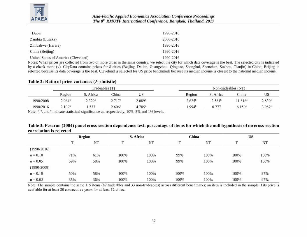
Asia-Pacific Applied Economics Association Conference Proceedings
The 8th RMUTP International Conference, Bangkok, Thailand, 2017
37
Dubai 1990-2016
Zambia (Lusaka) 2000-2016
Zimbabwe (Harare) 1990-2016
China (Beijing) 1990-2016
United States of America (Cleveland) 1990-2016
Notes: When prices are collected from two or more cities in the same country, we select the city for which data coverage is the best. The selected city is indicated
by a check mark (√). CityData contains prices for 8 cities (Beijing, Dalian, Guangzhou, Qingdao, Shanghai, Shenzhen, Suzhou, Tianjin) in China; Beijing is
selected because its data coverage is the best. Cleveland is selected for US price benchmark because its median income is closest to the national median income.
Table 2: Ratio of price variances (F-statistic)
Tradeables (T) Non-tradeables (NT)
Region S. Africa China US Region S. Africa China US
1990/2008 2.064b 2.329b 2.717b 2.089b 2.625b 2.581b 11.816c 2.830c
1990/2016 2.109b 1.537 2.606b 4.785c 1.994b 0.777 6.150c 3.987c
Note: a, b, and c indicate statistical significance at, respectively, 10%, 5% and 1% levels.
Table 3: Pesaran (2004) panel cross-section dependence test: percentage of items for which the null hypothesis of no cross-section
correlation is rejected
Region S. Africa China US
T NT T NT T NT T NT
(1990-2016)
α = 0.10 71% 61% 100% 100% 99% 100% 100% 100%
α = 0.05 59% 58% 100% 100% 99% 100% 100% 100%
(1990-2008)
α = 0.10 50% 58% 100% 100% 100% 100% 100% 97%
α = 0.05 35% 36% 100% 100% 100% 100% 100% 97%
Note: The sample contains the same 115 items (82 tradeables and 33 non-tradeables) across different benchmarks; an item is included in the sample if its price is
available for at least 20 consecutive years for at least 12 cities.

Asia-Pacific Applied Economics Association Conference Proceedings
The 8th RMUTP International Conference, Bangkok, Thailand, 2017
38
Table 4: Pesaran (2007) test with 0 lag: percentage of items for which the null hypothesis of unit root is rejected
Tradeables Non-tradeables All Items
[Region S. Africa China US] [Region S. Africa China US] [Region S. Africa China US]
(1990-2016)
α = 0.10 52% 56% 63% 56% 27% 39% 45% 36% 45% 51% 58% 50%
α = 0.05 44% 46% 51% 49% 15% 33% 39% 36% 36% 43% 48% 45%
(1990-2008)
α = 0.10 40% 51% 56% 56% 36% 45% 52% 39% 39% 50% 54% 51%
α = 0.05 32% 44% 46% 46% 27% 30% 42% 36% 30% 40% 45% 43%
Note: The sample contains the same 115 items (82 tradeables and 33 non-tradeables) across different benchmarks; an item is included in the sample if its price is
available for at least 20 consecutive years for at least 12 cities.
Table 5: Pesaran (2006) CCE estimates of convergence coefficient ρk in equation (7)
Region-average S. Africa benchmark China benchmark US benchmark
ρk Half-life (years) ρk Half-life (years) ρk Half-life (years) ρk Half-life (years)
(1990-2016)
T -0.384c 1.526 -0.394c 1.520 -0.432c 1.349 -0.416c 1.420
NT -0.308c 2.054 -0.320c 2.016 -0.358c 1.676 -0.346c 1.811
All items -0.362c 1.678 -0.373c 1.662 -0.411c 1.443 -0.396c 1.532
(1990-2008)
T -0.500c 1.095 -0.526a 1.039 -0.568b 0.921 -0.546c 0.977
NT -0.446c 1.255 -0.444c 1.297 -0.469c 1.220 -0.465c 1.178
All items -0.484c 1.141 -0.503a 1.113 -0.539b 1.007 -0.524c 1.034
Note: The values shown in the “ρk” columns in this table are averages of the estimates of the convergence parameter for the individual items in each group and
benchmark. The sample contains the same 115 items (82 tradeables and 33 non-tradeables) across different benchmarks; an item is included in the sample if its
price is available for at least 20 consecutive years for at least 12 cities.

Asia-Pacific Applied Economics Association Conference Proceedings
The 8th RMUTP International Conference, Bangkok, Thailand, 2017
39
Table 6: Robustness checks (I) – (III)
(I) Different lag length (II) Different test: IPS (2003) (III) Different sample selection
[Region
(1)
S. Africa
(2)
China
(3)
US]
(4)
[Region
(5)
S. Africa
(6)
China
(7)
US]
(8)
[Region
(9)
S. Africa
(10)
China
(11)
US]
(12)
Panel A: 1 lag
(1990-2016)
α = 0.10 22% 30% 38% 29% 45% 45% 47% 44% 36% 39% 49% 42%
α = 0.05 15% 21% 30% 20% 37% 30% 35% 34% 29% 32% 41% 33%
(1990-2008)
α = 0.10 17% 26% 33% 24% 48% 48% 53% 48% . . . .
α = 0.05 10% 18% 27% 17% 40% 38% 41% 41% . . . .
Panel B: 2 lags
(1990-2016)
α = 0.10 4% 11% 23% 17% 40% 36% 37% 35% 12% 16% 24% 21%
α = 0.05 3% 7% 16% 13% 29% 30% 26% 26% 7% 9% 19% 13%
(1990-2008)
α = 0.10 10% 11% 19% 12% 42% 41% 44% 36% . . . .
α = 0.05 6% 9% 11% 9% 30% 28% 31% 26% . . . .
Notes: In the robustness checks (I) and (II), the sample contains the same 115 items (82 tradeables and 33 non-tradeables) across different benchmarks just as in
Tables 3-5; an item is included in the sample if its price is available for at least 20 consecutive years for at least 12 cities. The sample in robustness check (III)
contains 135 items (95 tradeables and 40 non-tradeables); an item is included in this sample if its price is available for at least 14 consecutive years for at least 16
cities. In the robustness check (III), we do not consider shortened sample period of 1990-2008 because the loss of 9 time-series observations renders Pesaran (2007)
unit-root test inexecutable. Pesaran (2007) unit-root test in robustness check (I) and (III) accounts for cross-section dependence whereas IPS(2003) test in robustness
check (II) does not.

Asia-Pacific Applied Economics Association Conference Proceedings
The 8th RMUTP International Conference, Bangkok, Thailand, 2017
40
Table 7: Robustness check (IV): European Union (EU) sample; percentage of items for which
the null hypothesis of unit root in Pesaran (2007) test is rejected
Tradeables Non-tradeables All items
EU China US EU China US EU China US
α = 0.10 94% 91% 92% 60% 59% 70% 83% 81% 85%
α = 0.05 92% 87% 88% 57% 54% 58% 81% 77% 79%
Note: The sample period is 1990-2016. An item is included if its price is available for at least 21 consecutive years
for at least 19 out of 23 cities. This sample contains 119 items (84 tradeables and 35 non-tradeables); the items are
the same across the three price benchmarks.

Asia-Pacific Applied Economics Association Conference Proceedings
The 8th RMUTP International Conference, Bangkok, Thailand, 2017
41
Appendix
Table A1: List of items
Tradeables
Main
sample
Alternative
sample
(Robustness
check)
Food & Non-Alcoholic Beverages
White bread, 1 kg (supermarket)
Butter, 500 g (supermarket)
Margarine, 500g (supermarket)
White rice, 1 kg (supermarket)
Spaghetti (1 kg) (supermarket)
Flour, white (1 kg) (supermarket)
Sugar, white (1 kg) (supermarket)
Cheese, imported (500 g) (supermarket)
Cornflakes (375 g) (supermarket)
Yoghurt, natural (150 g) (supermarket)
Milk, pasteurised (1 l) (supermarket)
Olive oil (1 l) (supermarket) X
Olive oil (1 l) (mid-priced store) X
Peanut or corn oil (1 l) (supermarket)
Potatoes (2 kg) (supermarket)
Onions (1 kg) (supermarket) X
Onions (1 kg) (mid-priced store) X
Mushrooms (1 kg) (supermarket) X
Tomatoes (1 kg) (supermarket)
Carrots (1 kg) (supermarket)
Oranges (1 kg) (supermarket)
Apples (1 kg) (supermarket)
Lemons (1 kg) (supermarket)
Bananas (1 kg) (supermarket)
Lettuce (one) (supermarket)
Eggs (12) (supermarket)
Peas, canned (250 g) (supermarket) X
Tomatoes, canned (250 g) (supermarket) X
Tomatoes, canned (250 g) (mid-priced store) X
Peaches, canned (500 g) (supermarket) X
Peaches, canned (500 g) (mid-priced store) X
Sliced pineapples, canned (500 g) (supermarket) X
Sliced pineapples, canned (500 g) (mid-priced store) X
Beef: filet mignon (1 kg) (mid-priced store)
Beef: steak, entrecote (1 kg) (supermarket)
Beef: stewing, shoulder (1 kg) (supermarket)
Beef: roast (1 kg) (mid-priced store) X
Beef: ground or minced (1 kg) (supermarket)

Asia-Pacific Applied Economics Association Conference Proceedings
The 8th RMUTP International Conference, Bangkok, Thailand, 2017
42
Lamb: Stewing (1 kg) (supermarket) X
Chicken: frozen (1 kg) (mid-priced store) X
Chicken: fresh (1 kg) (supermarket) X
Frozen fish fingers (1 kg) (mid-priced store) X
Fresh fish (1 kg) (mid-priced store) X
Instant coffee (125 g) (supermarket)
Ground coffee (500 g) (supermarket) X
Tea bags (25 bags) (supermarket)
Drinking chocolate (500 g) (supermarket)
Coca-Cola (1 l) (supermarket)
Tonic water (200 ml) (supermarket)
Mineral water (1 l) (supermarket)
Orange juice (1 l) (supermarket)
Alcoholic Beverages & Tobacco
Wine, common table (750 ml) (supermarket)
Wine, superior quality (750 ml) (supermarket) X
Beer, local brand (1 l) (supermarket)
Beer, top quality (330 ml) (supermarket)
Scotch whisky, six years old (700 ml) (supermarket)
Gin, Gilbey's or equivalent (700 ml) (supermarket) X
Gin, Gilbey's or equivalent (700 ml) (mid-priced store) X
Cigarettes, Marlboro (pack of 20) (mid-priced store)
Cigarettes, local brand (pack of 20) (mid-priced store) X
Personal Care
Soap (100 g) (supermarket)
Laundry detergent (3 l) (supermarket)
Toilet tissue (two rolls) (supermarket)
Dishwashing liquid (750 ml) (supermarket)
Insect-killer spray (330 g) (supermarket)
Aspirins (100 tablets) (supermarket) X
Razor blades (five pieces) (supermarket)
Toothpaste with fluoride (120 g) (supermarket)
Facial tissues (box of 100) (supermarket)
Hand lotion (125 ml) (supermarket)
Shampoo & conditioner in one (400 ml) (supermarket)
Lipstick (deluxe type) (chain store)
Man's haircut (tips included) (average) N
Woman's cut & blow dry (tips included) (average) N
Furnishing & Household Equipment
Light bulbs (two, 60 watts) (supermarket)
Batteries (two, size D/LR20) (supermarket)
Frying pan (Teflon or good equivalent) (mid-priced store)
Electric toaster (for two slices) (supermarket)
Hourly rate for domestic cleaning help (average) N
Maid's monthly wages (full time) (average) N
Babysitter's rate per hour (average) N
Recreation & Culture

Asia-Pacific Applied Economics Association Conference Proceedings
The 8th RMUTP International Conference, Bangkok, Thailand, 2017
43
Compact disc album (average)
Television, colour (66 cm) (average)
Personal computer (64 MB) (average) X
Kodak colour film (36 exposures) (average)
Cost of developing 36 colour pictures (average) N
International foreign daily newspaper (average)
Daily local newspaper (average) N
International weekly news magazine (Time) (average)
Paperback novel (at bookstore) (average)
Four best seats at cinema (average) N X
Green fees on a public golf course (average) N
Hire of tennis court for one hour (average) N
Cost of six tennis balls eg Dunlop, Wilson (average)
Entrance fee to a public swimming pool (average) N
One good seat at cinema (average) N X
Clothing & Footwear
Laundry (one shirt) (standard high-street outlet) N
Dry cleaning, man's suit (standard high-street outlet) N
Dry cleaning, woman's dress (standard high-street outlet) N
Dry cleaning, trousers (standard high-street outlet) N
Men's business suit, two piece, medium weight (chain store)
Men's business shirt, white (chain store)
Men's shoes, business wear (chain store)
Socks, wool mixture (chain store)
'Women's dress, ready to wear, daytime (chain store)
Women's shoes, town (chain store)
Women's tights, panty hose (chain store)
Child's jeans (chain store)
Child's shoes, dresswear (chain store)
Child's shoes, sportswear (chain store)
Girl's dress (chain store)
Boy's dress trousers (chain store)
Housing, Water & Electricity
Furnished residential apartment: 1 bedroom (moderate) N
Furnished residential apartment: 2 bedrooms (moderate) N
Unfurnished residential apartment: 2 bedrooms (moderate) N
Unfurnished residential apartment: 3 bedrooms (moderate) N X
Telephone line, monthly rental (average) N X
Electricity, monthly bill for family of four (average) N
Transport
Low priced car (900-1299 cc) (low)
Compact car (1300-1799 cc) (low)
Family car (1800-2499 cc) (low)
Deluxe car (2500 cc upwards) (low)
Cost of a tune up (but no major repairs) (low) N
Annual premium for car insurance (low) N
Regular unleaded petrol (1 l) (average)

Asia-Pacific Applied Economics Association Conference Proceedings
The 8th RMUTP International Conference, Bangkok, Thailand, 2017
44
Taxi: airport to city centre (average) N
Hire car, weekly rate for lowest price classification (average) N X
Hire car, weekly rate for moderate price classification (average) N X
Restaurants & Hotels
Three-course dinner at top restaurant for four people (average) N
Business trip, typical daily cost N X
Hilton-type hotel, single room, one night including breakfast (average) N
Moderate hotel, single room, one night including breakfast (average) N
One drink at bar of first class hotel (average) N
Two-course meal for two people (average) N
Simple meal for one person (average) N
Fast food snack: hamburger, fries and drink (average) N
Education
American/English school: annual tuition, ages 5-12 (average) N
American/English school: annual tuition, ages 13-17 (average) N
American/English school: kindergarten annual fees (average) N
Medicare
Routine checkup at family doctor (average) N
Visit to dentist (one X-ray and one filling) (average) N
Notes: N=Non-tradeable. X=not included in the sample

Asia-Pacific Applied Economics Association Conference Proceedings
The 8th RMUTP International Conference, Bangkok, Thailand, 2017
45
Oil Palm, Land Use Change and Community Livelihoods in Indonesia: A Policy
Simulation Analysis
Dennis Mark Onuigbo a *, Bonar Marulitua Sinagab, Hariantoc
*aAgricultural Economics Study Program, Department of Resources and Environment Economics, Bogor Agricultural University, Dramaga – Bogor 16680, Indonesia. Email:
[email protected] bDepartment of Resources and Environment Economics, Bogor Agricultural University,
Dramaga – Bogor 16680, Indonesia cDepartment of Agribusiness, Bogor Agricultural University, Indonesiam
Abstract
Oil palm production has huge economic benefit. However, the business as usual approach of
increasing oil palm production has both environmental and social cost. We suggest that the
environmental cost can be seen through land use change and community vulnerability,
whereas, the social cost can be seen through livelihood changes. This study explored the
determinants of oil palm production and trade, land use change and community livelihoods;
and proffered evidence based policy alternatives that will ensure sustainability. To achieve this,
the econometric approach was used and the livelihood assets were defined based on review of
several livelihood frameworks. Historical data for 25 years (1990 – 2014) was analyzed using
the simultaneous equations model estimated with the two-stage least squares (2SLS) method
of estimation. The results showed that the policy instruments of increasing export tax,
secondary school enrolment ratio and workers wage played a major role in increasing
community livelihoods and reducing land use change. However, this policy has a tradeoff effect
as it resulted in a net national economic loss of Rp. 15.8 billion which may require sacrifice or
compensation for sustainability or for Pareto optimality to be attained.
Keywords: Oil palm production; trade; land use change; livelihoods; sustainability policy.

Asia-Pacific Applied Economics Association Conference Proceedings
The 8th RMUTP International Conference, Bangkok, Thailand, 2017
46
1. Introduction
Oil palm production has contributed to government revenue as the third largest export earner
after coal and petroleum with over $17.6 billion worth of crude palm oil exported in 2012. The
oil palm industries have employed over 3.7million people and have alleviated them from
poverty [1]. The numerous economic benefits of crude palm oil (CPO) production in Indonesia
motivate governments to make policies that targets increased production. The business as usual
approach to increasing CPO production is basically through forest, grassland or agricultural
land conversion. This increases the oil palm harvested area. This processes and practice has
both social and environmental cost. The social cost can be approached with livelihoods changes
in the community and the environmental cost through the concept of land use change.
Livelihood encompasses the ability of people to access the basic assets required for daily
human activities. Several livelihood frameworks identified five livelihood assets which
include: (1) Natural capital, (2) Human capital, (3) Social capital, (4) Physical capital and (5)
financial capital ([2]; CARE in [3]; [4]). These assets enable the community to overcome risk
or reduce vulnerability to changes, threats or shocks. Thus, a change in the optimum level of
the assets affects the livelihoods of the community. Changes in livelihoods are associated with
land use change (LUC). LUC can have both positive and negative effect on livelihoods and can
be defined by its cause. In agreement with several studies ([5]; [6]; [7]; [8]), LUC can be seen
in the conversion of rainforest, other agricultural lands, soil biomass/ peatlands into oil palm
plantation. It can result in increased economic benefit but with a tradeoff effect on environment
and community livelihoods. Climate change, flood, forest fire, water/air pollution and access
to basic livelihood assets are major environmental and livelihood concerns. Indonesia, the total
oil palm planted area increased at an annual average of 346,030ha, while the total forest area
decreased at an annual rate of 685,000ha. The increase in total planted area was accompanied
with an annual average increase in CPO production of about 1,985,710 million tons.
From the foregoing, it is pertinent to ensure that oil palm production and policies do not harm
the environment or reduce the livelihood of oil palm communities. So, we shall discuss at this
stage what determines oil palm production, domestic market, livelihoods in Indonesia and
suggest policies with better sustainability outcome. The major limitation of this work was
limited access to data; and at such, some were extrapolated. Because livelihood assets were
variables with mostly qualitative nature, derivation was necessary. However, this work will
provide an opportunity for empirical determination of land use change and livelihood changes
due to oil palm production. It will combine theories to test for endogenous behaviors and most
importantly create a room for further research or questions.
2. Determination of Livelihoods Assets
The different livelihood frameworks enabled the determination of the different livelihood
assets, the vulnerability context and land use change as endogenous. The determination is
necessary for the modeling as there are no direct data or standard measurement for the different
livelihoods assets available to the researcher. The derivation here were based on the sustainable
livelihoods frameworks discussed in [2], [3], and [4].
2.1 Community Access to Natural Capital
The community access to natural capital (CAN) is the ability of the community to benefit from
the natural resources such as land, water, soils, forest. When these resources are degraded, the
benefit for the communities diminishes. Mining, manufacturing and construction activities can
degrade the natural resource base of the community but they have almost immediate return or
economic benefit for the community. However, land degraded due to oil palm production may

Asia-Pacific Applied Economics Association Conference Proceedings
The 8th RMUTP International Conference, Bangkok, Thailand, 2017
47
not quickly transform to economic benefit for the community. From the foregoing, the
community access to natural capital will include the total land area not degraded by oil palm
production. It was given as thus:
CAN = (TAP - DLAP)/TAP *100 (1)
Where:
CAN = Community Access to Natural Capital (% of prov. land area un-degraded by
oil palm prod.)
TAP = Total land area (provinces) (1000 Ha)
DLAP = Oil palm degraded land area (provinces) (1000 Ha)
2.2 Community Access to Physical Capital
The community access to physical capital (CAP) is the ability of the community to utilize assets
that provide secure shelter, health care, education, energy, transportation, tools, equipment and
services provided through bank, grocery stores and related outlets. In the communities, the
access to electricity and households with roof main material provides the most importance
access to physical capital and thus the community access to physical capital was measured as
the weighted average of the percentage of households with roof main material and access to
electricity. It was given as thus:
CAP = (0.4*HHR + 0.6*HHAE) (2)
Where:
CAP = Community access to physical capital (% of household with main roof and
access to electricity)
HHR = Households by Roof Main Material (Non Sugar Palm Fiber/Other %)
HHAE = Household Access to Electricity (% of total household)
2.3 Community Access to Financial Capital
Community access to financial capital (CAF) is the ability of the community to earn income
from farm or off farm employment, trade activities, personal remittance or from bank credit.
The closest measure for this capital is the total own source revenue as data for remittance and
access to credit may not capture the poorer community members. Their access to credit can be
limited as most members are non-bankable since they may not have the basic requirements for
credit. Thus, the community access to financial capital can be measured by the per capita own
source revenue. It was given by:
CAF = (TOSR/POPP) (3)
Where:
CAF = Community access to Financial Capital (Rp.1000 /person)
TOSR = Total own source revenue oil palm prov. (Million Rp.)
POPP = Population of people in 1000 persons (Average population of oil palm prov.)
2.4 Community Access to Social Capital
Community access to social capital (CAS) is the ability of the households to make valuable
connections or network with other members of the community. This network either formal or
informal has the potential for economic benefit. However, the ability of households to make
such valuable connections depends on their status in the community. Poorer households find it
difficult to gain the required trust or meet basic fee required for meaningful cooperation
especially if it involves economic benefit. Households that live above the national poverty line
have better chances to make valuable connections that yield economic benefits. Thus a

Asia-Pacific Applied Economics Association Conference Proceedings
The 8th RMUTP International Conference, Bangkok, Thailand, 2017
48
community’s access to social capital can be seen in the number of people that live above the
poverty line. This was given as:
CAS = ((POPP-NPPL)/POPP)*100 (4)
Where:
CAS = Community Access to Social Capital (% of population above poverty line)
POPP = Population of people (1000persons oil palm prov.)
NPPL = Number of people that live below the poverty line (1000 persons)
2.5 Community Access to Human Capital
Community access to human capital is the ability of the community to possess the necessary
skills, knowledge, strength of mind and body that enable them to work for economic benefit.
This could be approached in several ways including approximating it for the population of
labour force within ages 15 – 64years with a certain education level. However, the population
of labour force at any education level may include people that are not economically active.
Thus, the community access to human capital is better approached with the labour force
participation rate which shows the percentage of labour force that are economically active.
According to the worldbank, these are the persons that supply labour for the production of
goods and services within a given period. This can be given by:
CAH = LFPR (5)
Where:
CAH = Community access to human capital (labour force participation rate %)
LFPR = Labor force participation rate for ages 15-64 (%)
3. Determination of Community Vulnerability
Community vulnerability/risk is the tendency of the community to experience disaster whether
natural or man-made. Disaster can be in form of disease outbreaks, famine, flood, landslides,
forest fire and earthquake. However, disaster like famine or disease can be more easily
controlled compared to environmental issues such as land slide, erosion, forest fire and
earthquake. Thus, the community vulnerability can be approached with the frequency of
occurrence of these environmental issues in the oil palm communities. This was given by:
CVR = D (6)
Where:
CVR = Community vulnerability (frequency of environmental disaster)
D = Frequency of disasters in form of landslide, forest fire, flood,
long dryness, tornado
The community capability and their access to the livelihood assets is influenced by policies.
Policies can decrease or increase land use change which influence the community vulnerability.
4. Determination of Land Use Change
Land Use Change (LUC) can be likened to any form of land conversion resulting from
human activities. These human activities include land conversion for agricultural or industrial
production. It was defined as human induced activities that results in greenhouse gas
emission [9]. In this work, land use change was determined as a percentage of the total
greenhouse gas emission. It was given as thus:
LUC = (TLE/TGHG)*100 (7)

Asia-Pacific Applied Economics Association Conference Proceedings
The 8th RMUTP International Conference, Bangkok, Thailand, 2017
49
Where:
LUC = Land Use Change (% of land use emissions (CO2))
TLE = Total land use emissions (gigagrams (CO2))
TGHG = Total Indonesia greenhouse gas emission (gigagrams (CO2))
To arrive at the models, the identified variables will be estimated and the econometric criteria
tested and validated. In the process of estimation and validation, irrelevant variables are
removed and the model re- specified to yield a robust model. Effort has been made to ensure
relevant variables are included through literature review and personal experience.
5. Economic Welfare
In a nation without government intervention in trade, the activities of producers and consumers
results to a market equilibrium. The market equilibrium represents the point of allocative
efficiency and this is the point where the economic surplus is maximized because consumers
and producers both get the highest benefit for the price they pay and accept. Thus, the economic
surplus measures the economic welfare for producers and consumers in a given nation.
However, since market equilibrium may not easily occur, government plays a role to maintain
a balance between consumer and producer surplus using tax or tariff. With tax or tariff,
government gets revenue from trade and could either make a transfer to cover for losses in
consumer surplus through special transfer programs like rice for the poor (RASKIN) or higher
education expenditure in Indonesia or involve in market operation to ensure better prices for
producers as it’s the case of the Logistics Bureau (Bulog) in Indonesia. With government
involvement in trade through tax or tariff, the net national surplus becomes the linear
summation of the producer surplus, the consumer surplus and government revenue. With tax
however, there will be a loss in total surplus known as the deadweight loss.
Let:
D = Demand curve
S = Supply curve
Pwtp = Maximum price consumers are willing to pay (Rp/tonne)
Pp = Price paid by consumers (Rp/tonne)
Pe = Market equilibrium or efficient price (Rp/tonne)
Pr = Price received by producers (Rp/tonne)
Pwta = Minimum price producers are willing to accept (Rp/tonne)
Qe = Equilibrium or efficient quantity (tonnes)
Qt = Quantity with tax (tonnes)
e0 = Market equilibrium
The economic surplus can be illustrated as in Figure 1:
Quantity (Q)
F
A
E
Qe
Pwtp
Price (P)
Pe
S
D
Pp
Pwta
Pa
Qt
C
D
B
e0

Asia-Pacific Applied Economics Association Conference Proceedings
The 8th RMUTP International Conference, Bangkok, Thailand, 2017
50
The producer surplus indicates the welfare gain by sellers from selling at a price (Pr) higher
than the minimum they are willing to accept (Pwta). On the other hand, consumer surplus
measures the gain a consumer gets from buying at a price (Pp) lower than he would be willing
to pay (Pwtp). It can be calculated as shown in table 1. Note that A to F in figure 1 can be
calculated with the area of the triangle which is ½ (Base x Height) or Base x Height for
rectangle. It can also be measured by the integration of the demand and supply function as:
𝑃𝑆 = ∫ 𝑄𝑠 (𝑃)𝑑𝑝𝑃𝑒
𝑃𝑟 (8)
and
𝐶𝑆 = ∫ 𝑄𝑑 (𝑃)𝑑𝑝𝑃𝑝
𝑃𝑒 (9)
Where:
PS = Value of producer surplus (Rp)
CS = Value of consumer surplus (Rp)
Qs = Quantity supplied (tonnes)
Qd = Quantity demanded (tonnes)
In this study we have applied the above concepts to measure the economic surplus of CPO
producers and consumers and the government revenue due from export tax. This will help us
to suggest the maximum (compensating variation) or minimum (equivalent variation)
compensation for making or not making a policy change. The concept of compensating
variation means the maximize compensation that should be paid for a change, whereas,
equivalent variation is the minimum compensation that one is willing to pay for a change not
to occur. As first used by [10], the compensating variation (CV) considers that a price increase
for a consumer who has a given level income will reduce the economic welfare of that
consumer. Therefore, the CV reflects the extra money which should be given to a consumer to
compensate for the price increase or a policy change.
6. Research Methodology
6.1 Data
Since oil palm is produced in selected provinces in Indonesia, this study have used data from
the seven major oil palm producing provinces to minimise overgeneralization for the
community livelihood assets. These were obtained from statistics Indonesia (BPS), World bank
subnational data (INDODAPOER). Data on community vulnerability were obtained from the
Indonesian national disaster management authority (BNPB). Data was also accessed from FAO
and USDA through Indexmundi. The data collected was annual and ranged from 1990 – 2014
(25 years). The selected oil palm communities (provinces) included Riau, Jambi, North and
South Sumatra, Central, East and West Kalimantan. These provinces are recognized as top oil
palm producing provinces in Indonesia.
6.2 Method
The simultaneous equations model was used to establish the relationship between endogenous
and exogenous variables while the Two Stage Least Square (2SLS) method of estimation was
used since the model was over-identified using the order condition [11]. This method curtails
errors of misspecification or other stochastic bias. The modeling went through stages of model
Figure 1 Consumer and Producer Surplus

Asia-Pacific Applied Economics Association Conference Proceedings
The 8th RMUTP International Conference, Bangkok, Thailand, 2017
51
specification, model identification, model estimation, model evaluation and validation. The
model comprised of 24 equations of which 19 are behavioral and 4 are identity equations.
Policy simulation was used to suggest policy alternatives with better sustainability outcome.
7. Model Specification
The model specification was drawn from theories, studies and the author’s experience. Among
others, the production function, demand and supply elasticities, understanding of international
trade and standard livelihoods frameworks have offered a lot to strengthen this work. Most of
these theories and various related studies have been discussed in [12]. The endogenous
relationship was summarized in figure 2.
[Insert Figures 2 around here]
The model specification was based on economic theories and standard livelihood frameworks.
The model comprised of 24 equations of which 19 are behavioral and 5 are identity equations.
Generally, the model comprise of six blocks which include; (1) Oil palm production block, (2)
Oil palm domestic market block, (3) International Trade block (4) Environment/emissions
block, (5) Community livelihoods block and (6) Community Vulnerability block. From figure
2, the arrow head shows the direction of influence flowing from the non-arrow head to the
arrow head. For instance, the diagram showed that Oil Palm Harvested Area (OHA) influenced
Land Use Change (LUC) and LUC influenced the community vulnerability/risk (CVR) and so
on.
8. Results of Model Validation
In this study the RMSPE and U-theil Coefficient noted earlier were used for the model
validation. The results of model validation have been shown in table 2.
[Insert Table 2 around here]
From the results of OLCL model validation in table 2, it was observed that from the 24
equations (both structural and Identity), only four (4) equations (16% of total equations) have
a RMSPE above 30. CPOM and CPOR equations performed badly. This was due to the high
disparity or fluctuation in the annual data of CPOM and CPOR resulting in a wide gap between
the regression line and the actual data. Meanwhile, only one (CPOM) equation (4% of total
equations) has a U-theil coefficient above 0.3. With the noted cases of high RMSPE and U-
theil, this validation result indicates that the predictive ability of the OLCL model is appropriate
for its intended use.
9. Results of Policy Simulation
From a historic overview of the oil palm policies mostly from 1993 Perkebunan Inti Rakyat
(PIR Trans) to date, the major policy instruments included the use of export tax, directed sales
of 80% of CPO production from government owned plantations to domestic market and the
expansion of oil palm harvested area.
The variable or windfall tax system was used. This tax system was based on the CPO
international price. Below an international CPO price of 700 $/MT, the export tax is zero (0%),
above 700 $/MT the tax increase by 1.5% for every 50$ increase and 2.5% for every 50$
increase above 950$/MT. However, above 1,250 $/MT it remains at a ceiling of 25%. From
the period simulated (2009-2014), the export tax has averaged at about 9% each year and in
some months when the international CPO price is low, the export tax is zero and its impact

Asia-Pacific Applied Economics Association Conference Proceedings
The 8th RMUTP International Conference, Bangkok, Thailand, 2017
52
high on government revenue such that the Jokowi government in 2015 intend to place a US
$50 levy and tax rate from $3-200 per ton for international prices in excess of US $750.
Another very important policy instrument was the use of land concession for oil palm
production. From the policy review, land allocation for oil palm plantation purposes have
continuously increased. And the Indonesian government has recently mentioned on a future
target of 6 million hectare expansion [13]. This will be roughly a 75% increase from the 2014
harvested area. This and other instruments have been simulated to find a more sustainable
policy. From over 50 policy scenarios tried, we selected to discuss four (5). Three (4) single
and one (1) combined policy scenarios. The aim was to determine the scenario that ensure
sustainable oil palm production, reduce land use change, improve community livelihoods and
reduce vulnerability.
The policy scenarios (S) presented here included:
S1: Increase CPO Export Tax by 5%
S2: increase oil palm harvested area by 15%
S3: increase net enrolment ratio to secondary school by 5%
S4: increase wage by 10%
S5: combination of s1, s3, and s4
The results of the policy simulation has been shown in table 3.
9.1 Effect of increase in CPO variable export tax by 5%
The simulation of increasing the variable export tax by 5% basically led to a decrease in export
quantity and CPO international market price. The behavior and values for the endogenous
variables are shown in table 3. From table 3, an increase in variable tax stimulated a 0.33% and
0.30% increase in CPO international market price and CPO export price respectively. This
resulted to a 0.04% (about 333,728 tonnes) increase in CPO domestic supply (CPOS) valued
at about which led to 0.02% drop in the real domestic price of CPO and a 0.04% increase in
the community access to physical capital. The increase in community access to physical capital
was due to increase in export tax which could stimulate higher government spending on basic
infrastructural development such as improving access to electricity which will increase the
peoples access to financial capital by 0.20% and a subsequent increase in social networks
though reduction in poverty by about 0.009%. From this policy of increasing export tax by
5%, some undesirable outcome included a 0.39% and 0.06% decrease in China and India CPO
import respectively. This led to a 0.005% drop in Indonesian CPO export. This policy however
is not desired because it has very little or no effect on land use change, community livelihood
assets and community vulnerability.
9.2 Effect of increasing Oil palm harvested area by 15% on Oil palm production, market, trade,
land use change, community livelihoods and community vulnerability
As this was the business as usual approach of increasing oil palm production, we simulated a
15% increase in oil palm harvested area even though the target was about a 75% (6million Ha)
increase from 2014 harvested area (Basri & Patunru. 2006 in Cervantes-Godoy et al. 2010).
The results of the can be seen in table 3.
[Insert Table 3 around here]

Asia-Pacific Applied Economics Association Conference Proceedings
The 8th RMUTP International Conference, Bangkok, Thailand, 2017
53
From table 3, a 15.00% increase in oil palm harvested area in the period simulated (2009-2014)
will increase oil palm production by 28.24% which will lead to an increase in CPO domestic
supply and CPO export by 55.29% and 15.21% respectively. This will reduce real domestic
price of CPO, CPO export price and CPO international market price by 16.67%, 6.5% and
4.89% respectively. The fall in CPO price will lead to a 0.11% increase in CPO domestic
demand, 0.88% and 5.30% increase in India and China CPO import respectively. The noted
changes will be accompanied by a 14.23% increase in the community access to financial
capital, a 0.61% and 0.66% increase in community access to physical and social capital
respectively. Even though this policy increased production and community access to financial
capital, It is not a desirable choice if concern for environment and overall community
livelihoods was considered serious. It is not a sustainable choice because of the huge trade off
on the community access natural capital, reducing it by about 34.30%. This also increased land
use change and community vulnerability/risk by 11.35% and 1.1% respectively.
9.3 Effect of increasing net secondary school enrollment ratio by 5%
With the thought that education will raise the quality of the human capital, we simulated the
effect of increasing the net secondary school enrolment ratio by 5% and the results have been
shown in table 3. From table 3, it was observed that a 5% increase in the net secondary school
enrolment ratio will increase the human capital by 0.28%, this will increase CPO production
by 0.28% due to better efficiency of labour. The resulting increase in production will lead to a
0.55% and 0.15% increase in CPO domestic supply and Indonesian CPO export respectively.
The increase in domestic supply and export will result in a 0.17% and 0.05% drop in CPO real
domestic price and CPO international market price respectively. This will be followed by a
0.05% and 0.01% increase in China and India CPO imports respectively. Note that, the ability
of Indonesia to influence the CPO international market price indicates that Indonesia is a big
country meaning that Indonesia has a large share in the CPO international market. This single
policy of increasing the net secondary school enrolment ratio by 5% is not a sustainable option
as it increased land use change by 0.12% and had no impact on community vulnerability/risk.
It also resulted in a 0.34% decrease in the natural capital due to the increase in CPO production
which resulted from a 0.18% increase in oil palm harvested area.
9.4 Effect of increasing plantation sector wage by 10%
The wage received or paid can serve as an important source of income for the plantation worker
and as an additional cost for the oil palm plantation. We simulated the increase in wage by 10%
and the results have been shown in table 3. From table 3, a 10% increase in wage will increase
the community access to human capital by 0.26%. This increase can be due to an increase in
the incentive to work which raise the number of people willing and ready to work from the
community and from outside the oil palm communities. However, this increase in wage
resulted in a higher cost of production, and reduced oil palm harvested area by 0.33% which
led to an increased access to natural capital by 0.64% and a 0.52% drop in total oil palm
production. Nevertheless, the decrease in production will result to a 1.03% and 0.28% decrease
in CPO domestic supply and Indonesian CPO export respectively. The decrease in Indonesian
CPO domestic supply and export will result to a 0.31% and 0.09% increase in CPO domestic
price and International price respectively. This policy was appropriate for reducing land use
change and community vulnerability by 0.12% and 0.02%. However, it was not the most
desirable because it reduced the community access to physical, financial and social capital by
0.005%, 0.11%, and 0.005%. This is a double tragedy since it reduced oil palm production
without a full positive impact on all the livelihood assets.

Asia-Pacific Applied Economics Association Conference Proceedings
The 8th RMUTP International Conference, Bangkok, Thailand, 2017
54
9.5 Effect of policy combination of increasing CPO variable export tax by 5% (S1), increasing
secondary school net enrolment ratio by 5% (S3) and increasing plantation sector wage by
10% (S4)
At several trials, we attempted to harness the combined potential of the single policy scenarios.
Here, we simulated the combined (S5) effect of increasing CPO variable tax by 5% (S1),
increasing secondary school net enrolment ratio by 5% (S3) and increasing plantation sector
wage by 10% (S4). The results are shown in table 3. From table 3, S5 combination had a more
desirable effect. A trade off effect existed in the production block, environment/ emissions
block and community livelihoods block. This policy decreased total oil palm production by
0.24% all things been equal but with a consequent reduction in land use change and community
vulnerability by 0.06% and 0.02% respectively. This also led to an improvement in all the
community livelihood assets which are necessary for their daily living and survival. The
improvement in human and natural capital was more with a 0.54% and 0.30% increase,
whereas, physical, financial and social capital increased by 0.03%, 0.09% and 0.004%
respectively.
10. Results of economic surplus
The effect of the different policy scenarios were tested on the economic welfare of CPO
producers and consumers, and on government revenue from tax. This will enable the estimation
of the net national surplus due to the policy changes. The results of economic surplus for year
2009 -2014 were given in table 4.
[Insert Table 4 around here]
From the results of simulating economic surplus in table 4, the business as usual approach to
oil palm production (increasing oil palm harvested area by 15%) will result in a gain in net
national surplus of about Rp. 160.5 billion over 6years (2009-2014). Increasing the variable
export tax by 5% resulted in a net national loss of about Rp. 174 million over a period of 6years.
This is due to a higher percentage decrease in CPO export with a relatively little increase in
tax. Thus, resulting in a loss in government revenue from tax; a Rp. 49400 gain in producer
surplus and an Rp. 12880 gain in consumer surplus due to higher international market price for
the producer and lower domestic price for the consumer. This phenomenon indicates that the
oil palm producers are loss averse which represent the rational behavior of producers generally.
An increase in the secondary school net enrolment ratio by 5% was positive to the net national
surplus with a gain of about Rp. 3.1 billion. This was because an increase in the secondary
school net enrolment increased the human capital, oil palm production and Indonesian CPO
export. An increase in the workers wage by 10% was negative to the net national surplus with
a loss of about Rp. 2.97 billion. This was because an increase in workers wage decreased
Indonesian CPO production and export which decreased producers surplus and raised the real
domestic price of CPO. As expected, the S5 combination was negative to net national surplus,
reducing it by Rp. 15.8 billion. This helped to emphasize the tradeoff effect between economic
and environmental/ social concerns.

Asia-Pacific Applied Economics Association Conference Proceedings
The 8th RMUTP International Conference, Bangkok, Thailand, 2017
55
11. Conclusion
From the study shows a tradeoff effect between oil palm production and land use change with
the business as usual approach of increasing oil palm harvested area. S1 – S5 are different
policy scenarios tried. The figure 3 illustrates the in a box.
A lot more scenarios can be tried until the point of pareto optimal. However, with over 60
scenarios tried so far, no policy could ensure an improvement in one or two without making at
least one worse off. S5 did better for land use change, livelihood assets and vulnerability but
with economic loss due to a slight reduction in oil palm production. The compensating variation
(CV) used by [9] can be explored to service the net national loss in table 4. Generally, as
expected, a 15% increase in oil palm harvested land increased oil palm production by 28.24%.
The increased production led to a 14.23%, 0.61%, 0.66% increase in the community access to
financial, physical, and social capital respectively. It also led to a gain in net national surplus
of about Rp. 160.5 billion with a consequent 11.35% increase in land use change which resulted
in a 1.1% increase in community vulnerability.
This could be attributed to the resultant 34.30% decrease in the community access to natural
capital. Contrary to expectation, a 5% in increase in the net secondary enrolment ratio increased
human, physical, financial and social capital by 0.28%, 0.005%, 0.11% and 0.005%
respectively but had no effect on community vulnerability. It instead, resulted in a 0.34%
Figure 2 OLCL Sustainability Box
S5
Trade off
S4 S1
S2 S3
Pareto Optimal =
Pareto improvement
+
Compensating Variation
Pareto improvement
Description:
S1-S5 = Selected policy scenarios (Table 14)
Obj: = Objective
Livelihood + = Objective to increase community livelihood assets (CAN,
CAP, CAF, CAS, CAH)
CVR - = Objective to decrease community vulnerability (CVR)
Land use change - = Objective to decrease land use change
- Or + = Decrease or increase
Obj:
Livelihood +
CVR -
Obj:
Land Use Change -
Obj:
Oil Palm Production +
Social Environment
Economic

Asia-Pacific Applied Economics Association Conference Proceedings
The 8th RMUTP International Conference, Bangkok, Thailand, 2017
56
decrease in natural capital and a 0.11% increase in land use change. More so, a 5% increase in
export tax was against expectation as it decreased the net national surplus by Rp. 174 million.
This indicates a loss aversive behavior of producers who will react by reducing a larger quantity
exported relative to a small increase in export tax. This was positive to both consumer and
producer surplus as they gained from lower domestic price and higher international prices
respectively. In the same vein, an increase in workers wage did not improve all livelihoods
assets as expected but was appropriate for reducing land use change and vulnerability.
Increasing wage by 10% was good in increasing human and natural capital by 0.25% and 0.64%
respectively but reduced the community access to physical, financial and social capital by
0.009%, 0.20% and 0.01% respectively.
12. Policy Recommendation
Through policy simulation aimed at solving the objective for sustainable oil palm production,
reduction in land use change and improvement in community livelihoods, we recommend a
policy combination of increasing the variable export tax by 5%, increase secondary school
enrolment by 5% and increasing plantation worker wage by 10% within a six year period as
options for sustainability. These policy instruments will not yield the desired outcome if used
as a single instrument. They are better when combined. The rationale for the combination was
that an increase in export tax, will increase domestic supply and decrease domestic CPO price
which kept production relatively stable or low, whereas, an increase in secondary school
enrolment will increase the quality and quantity of human capital whose ability and knowledge
will help to increase oil palm production in a more sustainable way as they may serve as labour
for the plantations or be advocates for good environmental and social practices. On the other
hand, an increase in wage will raise the cost of production, and limit the need to expand
harvested area and thus reduce land use change. The purpose for combining the instruments is
to make up for their individual undesirable impact. Furthermore, the economic surplus
calculation indicates a national economic loss due to an improvement in environmental and
social concerns, but an economic gain due to the business as usual production. The economic
loss can be a national sacrifice since environmental and social cost are more expensive; or
requires compensation by nations or groups with environmental and social concerns. The
compensation will make up for the economic loss due a slight reduction in production and an
improvement in community livelihoods accompanied with a decrease in land use change and
community vulnerability.
Acknowlegement
Special thanks to the faculty of economics and management, Bogor Agricultural University
(IPB), the IPB directorate of students affairs (DITMAWA) and the IPB graduate school
(pascasarjana) for the financial support provided for the presentation of this work at Bangkok-
Thailand. Sincere appreciation to the Indonesian government for the developing countries
partnership scholarship (KNB) awarded for my masters program.

Asia-Pacific Applied Economics Association Conference Proceedings
The 8th RMUTP International Conference, Bangkok, Thailand, 2017
57
References
[1] Schuster Institute for Investigative Journalism. Indonesia’s Palm Oil Industry.
Brandeis University, USA., 2015.
[2] [FAO] Food and Agriculture Organization. Socio-Economic and Livelihood
Analysis in investment planning. Policy Learning 2008.
[3] K. Westley, V Mikhalev. The Use of Participatory Methods for Livelihood
Assessment in Situations of Political Instability: A Case Study from Kosovo.
Working Paper 190. Overseas Development Institute 111 Westminster Bridge Road
London (UK) SE1 7JD ISBN: 0 85003 628 3, 2002.
[4] J. Murray, F Mary. Women in Transition Out of Poverty. Toronto: Women and
Economic Development Consortium. 2001.
[5] B. Wicke, R. Sikkema, V. Dornburg, A. Faaij. Exploring Land Use Changes and
the Role of Palm Oil Production in Indonesia and Malaysia. Journal of Land Use
Policy 28 (2011) 193–206 doi:10.1016/j.landusepol.2010.06.001.
[6] K. Obidzinski, R. Andriani, H. Komarudin, A. Andrianto. Environmental and
social impacts of oil palm plantations and their implications for biofuel production in
Indonesia. Ecology and Society 17(1): 25. http://dx.doi.org/10.5751/ES-04775-170125
2012.
[7] Budidarsono S, Dewi S, Sofiyuddin M, Rahmanulloh A. Socioeconomic Impact
Assessment of Palm Oil Production. Technical Brief No. 27: palm oil series. Bogor
(ID), World Agroforestry Centre - (ICRAF), SEA Regional Office. 4p, 2012.
[8] N Wilms-Posen, M Boomkens, S. d’Apollonia, A. Klarer, E.M Kraus, L.L Tynell.
Land-Use and Livelihoods – A Malaysian Oil Palm Scheme
and its Social and Ecological Impacts. The Journal of Transdisciplinary Environmental
Studies 13(2), 2014.
[9] IPCC - Intergovernmental Panel on Climate Change. Land Use, Land Use Change and
Forestry. 2015.
[10] J.R Hicks. Value and Capital: An Inquiry into some Fundamental Principles of
Economic Theory. Oxford: Clarendon Press, 1939.
[11] A. Koutsoyiannis. Theory of Econometrics: An Introductory Exposition of
Econometric Methods. (2nd ed). The Macmillan Press Ltd, Great Britain. 1977
[12] D.M Onuigbo, S.M Bonar, Harianto. 2017. Oil Palm Policy, Land Use Change and
Community Livelihoods (OLCL) In Indonesia: A Sustainability Framework. A paper
accepted on the 10th November, 2016. International Journal of Environmental Science
and Development (ISSN: 2010-0264)
[13] M Basri, A Patunru. Survey of Recent Developments. Bulletin of Indonesian Economic
Studies, 295-319, 2006.

Asia-Pacific Applied Economics Association Conference Proceedings
The 8th RMUTP International Conference, Bangkok, Thailand, 2017
58
Figure 3 Oil Palm Policy, Land Use Change and Community Livelihood (OLCL)
Model.

Asia-Pacific Applied Economics Association Conference Proceedings
The 8th RMUTP International Conference, Bangkok, Thailand, 2017
59
Table 1 Economic Welfare With Tax and Without Tax
Without tax With tax Change
Consumer surplus D+E+F F -(D+E)
Producer surplus A+B+C A -(B+C)
Government revenue None B+E +(B+E)
Net National surplus A+B+C+D+E+F A+B+E+F -(C+D)
Table 2 Results of Model Validation
VARIABLE RMSPE
U-
THEIL LABEL
OHA 0.47 0.00 Oil palm harvested area (1000 Ha)
OPY 7.18 0.04 Oil palm yield (MT/Ha)
TOPP 7.29 0.03 Indonesia total CPO production (1000MT)
CPOR 493.20 0.18 Indonesia CPO stock (1000MT)
CPOS 38.18 0.15 Indonesia CPO supply (1000MT)
CPOD 4.32 0.02 Indonesia CPO domestic demand (1000MT)
CPODF 6.21 0.03 CPO demand for food use (1000MT)
RDPC 10.38 0.05 Real domestic price of CPO (Rp/Kg)
CPOX 4.57 0.02 Indonesia CPO export (1000MT)
MCX 2.64 0.01 Malaysia CPO export (1000MT)
TWCX 2.49 0.01 Total World CPO Export (1000 MT)
CPOM 799.60 0.35 Indonesia CPO import (1000MT)
CCM 7.70 0.04 China CPO Import in (1000 MT)
ICM 4.96 0.02 India CPO Import (1000 MT)
TWCM 2.49 0.01 Total World CPO Import (1000 MT)
CIMP 5.72 0.03 CPO international market price (USD/MT)
CEP 16.99 0.09 CPO Export Price (USD/tonne)
LUC 9.35 0.05 Land Use Change ( % of land use emission (CO2))
CAN 82.70 0.19
Community Access to Natural Capital (% of prov. land area
un-degraded by oil palm prod.)
CAP 2.19 0.01
Community access to physical capital (% of household with
main roof and access to electricity)
CAF 20.90 0.09 Community Access to Financial Capital (Rp.1000 per capita)
CAS 2.47 0.01 Community Access to Social Capital (% of pop. above poverty line)
CAH 0.44 0.00 Community Access to Human Capital ( labour force participation rate %)
CVR 21.69 0.14 Community Vulnerability/Risk (frequency of environmental disaster)
Source: Data Analysis

Asia-Pacific Applied Economics Association Conference Proceedings
The 8th RMUTP International Conference, Bangkok, Thailand, 2017
60
Table 3 Results of Policy Simulation 2009 - 2014
Variables Base s1 s2 s3 s4 s5
Oil palm harvested area (1000 Ha) 7465.
1
0.000 15.00
0
0.175 -
0.330
-
0.154
Oil palm yield (MT/Ha) 3.640
9
0.000 11.46
4
0.088 -
0.173
-
0.085
Indonesia total CPO production (1000 MT) 27444
.1
-
0.001
28.24
4
0.277 -
0.524
-
0.248
Indonesian CPO supply (1000 MT) 8343.
2
0.036 55.29
2
0.548 -
1.034
-
0.452
Indonesian CPO domestic demand (1000 MT) 7156.
5
-
0.011
0.068 0.000 -
0.003
-
0.013
CPO demand for food use (1000 MT) 4703.
8
-
0.017
0.104 0.002 -
0.002
-
0.019
Real domestic price of CPO (Rp/Kg) 11398
.1
-
0.016
-
16.66
5
-
0.165
0.311 0.131
Indonesian CPO export (1000 MT) 19949
.1
-
0.017
15.21
2
0.149 -
0.281
-
0.150
Malaysian CPO export (1000 MT) 17445 0.008 -
0.11
6
-
0.001
0.002 0.009
Total World CPO Export (1000 MT) 39243
.9
-
0.005
7.682 0.075 -
0.142
-
0.072
China CPO Import in (1000 MT) 6176.
2
-
0.389
5.393 0.045 -
0.087
-
0.431
India CPO Import (1000 MT) 7717.
3
-
0.060
0.876 0.008 -
0.017
-
0.067
Total World CPO Import (1000 MT) 28936
.4
-
0.099
1.421 0.012 -
0.023
-
0.111
CPO international market price (USD/MT) 808.4 0.334 -4.886 -
0.049
0.087 0.371
CPO Export Price (USD/tonne) 504.2 0.298 -6.525 -
0.060
0.119 0.357
Land Use Change ( % of land use emission (CO2)) 169.1 0.000 11.35
4
0.118 -
0.237
-
0.059
Community Access to Natural Capital (% of prov. land area un-
degraded by oil palm prod.)
20.33
76
0.001 -
34.30
2
-
0.337
0.636 0.301
Community access to physical capital (% of household with main
roof and access to electricity)
45.91
36
0.039 0.608 0.005 -
0.009
0.034
Community Access to Financial Capital (Rp.1000 per capita) 353.5 0.198 14.22
9
0.113 -
0.198
0.085
Community Access to Social Capital (% of population above
poverty line)
89.31
37
0.009 0.658 0.005 -
0.010
0.004
Community Access to Human Capital ( labour force participation
rate %)
70.05
04
0.000 -0.002 0.284 0.256 0.539
Community vulnerability/Risk ( frequency of environmental
disaster)
427.1 0.000 1.100 0.000 -
0.023
-
0.023

Asia-Pacific Applied Economics Association Conference Proceedings
The 8th RMUTP International Conference, Bangkok, Thailand, 2017
61
Table 4 Results of Economic Surplus for year 2009 - 2014 Business as usual Improvement
Surplus in Rp.1000 S1 S2 S3 S4 s5
Producer 49.40 52126.19 515.91 -971.45 -408.88
Consumer 12.88 13593.77 134.54 -253.34 -106.63
Govt Revenue -174436.98 160413299.54 1569932.78 -2965428.58 -1580504.71
net national
surplus
-174374.69 160479019.51 1570583.23 -2966653.37 -1581020.23
Description: S1: increase Export tax by 5%;
S2: increase oil palm harvested area by 15%;
S3: increase net enrolment ratio to secondary school by 5%;
S4: increase wage by 10%;
S5: combination of s1, s3, and s4

Asia-Pacific Applied Economics Association Conference Proceedings
The 8th RMUTP International Conference, Bangkok, Thailand, 2017
62
Simultaneous Determinants of Fiscal Policy, Monetary Policy, Income Inequality, Trade,
Domestic Credit to Private Sector and Economic Growth: Case of Emerging Market
Economy
Dipyaman Pal*1, ArpitaGhose**
*Bethune College, Kolkata, West Bengal, India; Email: [email protected]
**Jadavpur University, Kolkata, India; Email: [email protected]
Abstract
A panel-VAR model is used to determine the existence of simultaneous-relationship between
economic-growth, income-inequality, fiscal- policy, monetary-policy, domestic-credit to private
sector and total-trade of the 13 emerging market economy (EMEs) as a group for the period 1980-
2010. After establishing the existence of simultaneity between the above relationships a
simultaneous panel model has been formulated and estimated incorporating the non-linearity
among the variables as suggested by the existing literature. An inverted U-shape relationship is
evident between (i) economic-growth, income-inequality and total-trade, in economic-growth
equation, (ii) income-inequality, economic growth and per-capita income in income-inequality
equation, (iii) total-trade and economic-growth, in total-trade equation and (iv) monetary-policy
and fiscal-policy, in monetary-policy equation. Also, a U-shaped relationship between monetary-
policy and fiscal- policy is observed in fiscal-policy equation. Thus, the existence of a two-way
non-linear relationship is highlighted between economic-growth, income-inequality, total-trade
and monetary-policy. Apart from these non-linear relationships, positive and significant effect of
(i) gross capital formation, inflation, population growth, human capital, fiscal policy, monetary
policy and domestic-credit to private sector on economic-growth; (ii) civil liabilities on income
inequality; (iii) gross capital formation and inflation on total trade; (iv) total trade, population
growth 65 years and above, political system on fiscal-policy; (v) per-capita GDP, total reserves,
fiscal-policy and domestic-credit to the private-sector on monetary-policy and (vi) money-supply
and gross domestic savings on domestic-credit to the private sector is highlighted. Also, negative
and significant effect of (i) fiscal-policy on income-inequality; (ii) income-inequality on fiscal
policy; (iii) total-trade on domestic-credit to the private-sector is revealed.
Keywords: Economic Growth, Fiscal Policy, Monetary Policy, Income Inequality, Panel-VAR,
Panel Unit Root
1 Corresponding author

Asia-Pacific Applied Economics Association Conference Proceedings
The 8th RMUTP International Conference, Bangkok, Thailand, 2017
63
1. Introduction
The reduction of economic disparities is one of the most challenging public policy topics in
macroeconomic literature. An innermost concern of this debate is that whether the role government
policies may play a vital role in reducing economic inequalities, and determining the effects on
economic growth rate (Bénabou, (2000, 2002, 2005) and Seshadri and Yuki (2004)) or not.
The political economy literature reveals the theoretical background of the empirical models, where
fiscal policy, inequality and growth are jointly determined in democratic societies. These political
economy models of inequality and growth pointed out that the fiscal policy can play a major role
in explaining the development of both macro aggregates. In this context, fiscal policy which is an
endogenous variable reflects, through political processes, the voters' preferences for income
distribution (each individual behaves like an economic agent and a citizen who votes on the
distributive policies) (Drazen, 2000; chapter 11 and Persson and Tabellini, 2000; chapter 14).
Under the assumption of perfect capital markets early political economy models shows a negative
relationship between inequality and growth (Alesina and Rodrik, 1994, Bértola, 1993 and Persson
and Tabellini, 1994). This traditional idea does not seem very supportive by the later empirical
contributions using cross-country data. Recently, the political economy literature wanted to loosen
up the main assumptions of the abovementioned approaches. Bénabou (2000) argues how
countries with similar preferences and technologies as well as equal democratic political systems,
can however make very different choices with respect to fiscal policies. Muinelo-Gallo and Roca-
Sagalés (2013) analysed the relationship between income inequality and economic growth through
fiscal policy. They presented and estimated two systems of structural equations with error
components through which gross income inequality determines different fiscal policy outcomes,
which subsequently affects the evolution of economic growth and net income inequality. The
empirical results, obtained using an unbalanced panel data of 21 high-income OCDE countries
during the period 1972–2006, suggested that gross income inequality is a significant determinant
of fiscal policy outcomes. Additionally, the results showed that distributive expenditures and direct
taxes may produce significant reductions in GDP growth and net income inequality reflecting the
standard efficiency–equity trade-off associated to certain fiscal policy measures. Finally, the
results also indicated that the most adequate fiscal policy strategy in a context of fiscal
consolidation is to cut non distributive expenditure, since this could increase GDP growth while
reducing income inequality.
Earlier studies like Bénabou (2000); Muinelo-Gallo and Roca-Sagalés (2013) etc have considered
the joint determination of economic growth, income inequality and fiscal policies. But the
limitations of these studies are as follows: First of all, they did not take into account the effect of
monetary policy on growth. In fact there are some literature which reflects the joint relationship
between economic growth, government expenditure and money supply (Albatel (2000) for Saudi
Arabia and Mohammad et. al. (2009) for Pakisthan). Mohammad et. al. (2009) argued that public
expenditure and inflation are negatively related to economic growth in long run while M2 is
positively impacts on economic growth in long run. The reason behind the negative association
among public expenditure, inflation and economic growth is the most of public expenditure is non
development and inflation is due to adverse supply shock (cost push inflation) in case of Pakistan.
Demary (2004) found that unanticipated money growth affects real output and employment in case
of West Germany. Georgantopoulos and Tsamis (2013) established the short and long term
relationship between money supply, inflation and economic growth in Cyprus and Tabar et.al
(2016) for Iran. Georgantopoulos and Tsamis (2013) Tabar et.al (2016) and the studies argued that

Asia-Pacific Applied Economics Association Conference Proceedings
The 8th RMUTP International Conference, Bangkok, Thailand, 2017
64
public expenditures promote economic development. Monir et al. (2015) established that the
money supply in the banking system of Bangladesh has a positive impact on the following
macroeconomic variable: nominal interest rate, bank rate, and remittance, but has an adverse
consequence on the following variables: such as interest rate and deposit inflation.
Secondly, domestic credit to private sector is also a major determinant of economic growth (Ea et
al., 2015; Okafor et al., 2016 etc.). The interrelationship between financial sector development and
economic growth was established by Dudian et al. (2013) for the region central and eastern Europe
taking into account a panel of eight countries from the region and by Alkhuzaim( 2014) for Qatar.
Dudian et al. (2013) measured financial sector by broad money growth (annual%), domestic credit
to private sector (% GDP), domestic credit to private sector (% GDP) annual growth, interest rate
spread (lending rate minus deposit rate,%) and nonperforming loans (% total loans), while
Alkhuzaim( 2014) measured financial sect by three alternative indicators: a broad money supply
(M2) to GDP ratio, bank credit to the private sector as ratio to GDP, and domestic credit provided
by bank sector as ratio to GDP. The economic growth is measured by the growth rate of real GDP
by both Dudian et al. (2013) and Alkhuzaim( 2014). Dudian et al. (2013) found that increase
nonperforming loans and interest rate spreads negatively affect economic growth and increase in
domestic credit to private sector negatively affect GDP growth, but increase its growth rate
positively affects GDP. Also broad money growth is less relevant for economic growth.
Alkhuzaim( 2014) argued that a positive long-run equilibrium relationship exists between all three
financial development indicators and the growth rate of real GDP. Arıç (2014) found that Domestic
Credit to Private Sector as % of GDP affects economic growth negatively, Capitalization Ratio
and Money and Quasi Money M2 as % of GDP affect growth positively. Ea et al (2015) obtained
a negative relationship between domestic credit and economic growth for eight countries in
ASEAN member states excluding Myanmar and Lao PDR. Okafor et al. (2016) established a
unidirectional causal relationship between deposit money bank credit and economic growth in
Nigeria. However, the linkage between domestic credit to private sector and economic growth are
missing in Muinelo-Gallo and Roca-Sagalés (2013).
Thirdly, Alihodžić (2016) etc also suggests that domestic credit to private sector depends on the
money supply of the economy. It is well known fact that one of the major determinants of money
supply is domestic credit to private sector. Thus there exists a bi-directional relationship between
money supply and domestic credit to private sector. The possibility of the existence of linkage
between money supply and domestic credit to private sector was not considered by Muinelo-
Gallo and Roca-Sagalés (2013).
Fourthly, there also exist some views in the literature regarding the causal direction of the effects
of trade openness on economic growth. Michaely (1977), Feder (1982), Marin (1992), Thornton
(1996) found that countries exporting a large share of their output seem to grow faster than others.
Grossman and Helpman (1991), Rivera-Batiz and Romer (1991), Romer (1990) hypothesize that
expanded international trade increases the number of specialized inputs, increasing growth rates
because economies become open to international trade. Buffie (1992) considers how export shocks
can produce export-led growth (Ribeiro Ramos, 2001). The export-led growth hypothesis (Zuniga,
2000) broadly focuses on whether a country is better served by orienting trade policies to export
promotion or import substitution. The favorable impact of exports on economic growth has been
well established in the literature (Kruger, 1975; Balassa, 1978; Williamson, 1978; Bhagawati,

Asia-Pacific Applied Economics Association Conference Proceedings
The 8th RMUTP International Conference, Bangkok, Thailand, 2017
65
1982; Srinivasan, 1985; Love and Chandra, 2004; Mah, 2007; Ziramba, 2011 among others). In
the Growth Led Export (GLE) case, export expansion could be stimulated by productivity gains
which caused by increase in domestic levels of skilled-labor and technology (Bhangwati, 1988;
Krugman, 1984). Neoclassical trade theory typically argues that the causality that runs from home-
factor endowments and productivity to the supply of exports (Findlay, 1984). The product life
cycle hypothesis developed by Vernon (1996) has also concerned considerable attention among
international trade theorists in recent years. Segerstrom et al. (1990), for example, use the product
life cycle hypothesis as a basis for analyzing north_south trade in which research and development
competition between firms determines the rate of product innovation in the north (Ribeiro Ramos,
2001). The third alternative is that of import-lead growth (ILG) shows that economic growth could
be driven primarily by growth in imports (Coe and Helpman, 1995). Growth in imports can serve
as a medium for the transfer of growth-enhancing foreign R&D knowledge from developed to
developing countries (Lawrence and Weinstein, 1999; Mazumdar, 2000). The most interesting
economic scenarios suggest a two-way causal relationship between growth and trade. According
to Bhagwati (1988), increased trade produces more income (increased GDP), and more income
facilitates more trade. So, the result suggests a ‘virtuous circle’. This type of feedback has also
been noted by Grossman and Helpman (1991) in their models of north_south trade. But Muinelo-
Gallo and Roca-Sagalés (2013) did not take into account possible bi-directional linkage between
trade and economic growth.
It may also be mentioned that, only a limited number of studies are available for a panel of
countries (Muinelo-Gallo and Roca-Sagalés (2011b) for OECD). More specifically, there is dearth
in studies which estimated the simultaneous relationship for the emerging market economy (EME)
as a group. In 1981, Agtmael defined an emerging market economy (EME) as a developing
economy with low to middle per capita income, pursuing reform programmes in the market-
oriented line and gradually becoming as significant players in the global economy (Agtmael 2007).
The potential causes for the creation of an EME are the failure of state-led economic development,
its tremendous negative impact and the need for capital investment which had pushed those
countries to adopt open door policies, to replace their traditional state interventionist policies,
undertake economic and political reforms and to change from the state being in charge of the
economy to facilitate economic growth along market-oriented lines. Hence it will be interesting to
see what kind of relationship hold among the above mentioned variables for the EME as a group.
Therefore, the first objective of the paper is to check whether there exists any long run and short
run simultaneous relationship between economic growth, inequality, fiscal policies, monetary
policies, domestic credit to private sector and total trade or not using a VAR frame work by
considering a panel of 13 EME [Brazil (BRA), Chile (CHL), China (CHN), Colombia (COL),
Ecuador (ECU), India (IND), Malaysia (MYS), Mexico (MEX), Morocco (MAR), Pakistan
(PAK), Philippines (PHL), South Africa (ZAF) and Venezuela (VEN) (Based on The International
Monetary Fund classification)] over the period of 1980-2010. In order to test long run relationship
in the first step panel unit root test is applied by Levin and Lin (1992, 1993) and Im, Pesaran, and
Shin (IPS) method. The results of panel unit root test by LLC and IPS method are presented in
Table-1. From the results it can be concluded that by both method all the variables are stationary
at their level. So, all the series are integrated of order 0. So, one may not be able to run the panel
co-integration analysis to find out the long run relationship between these variables. However, one
can find out the short run relationship between the variables by applying panel VAR model.

Asia-Pacific Applied Economics Association Conference Proceedings
The 8th RMUTP International Conference, Bangkok, Thailand, 2017
66
All the results of panel VAR model are presented in Table-2 to Table-7. From the results of the
panel VAR model it can be concluded that there exists short run relationship between Economic
Growth, Income Inequality, Fiscal Policy, Monetary Policy, domestic credit to private sector and
total tread2.
The perusal of the literature suggests that the relationship between these above mentioned variables
can in-fact be of non-linear type (Henderson and Wang (2015); Lin et. al (2014); Kim and Lin
(2009); Cotarelli, et. al. (2005); etc). However, such non-linearity has not been captured in the
above results as described in Table 2 to Table 7. The perusal of the literature suggests that there is
dearth in the studies capturing the existence of non-linearity among the endogenous variables in a
simultaneous panel setup. The present paper adds to the literature in this direction. Therefore, to
take into account of this fact a simultaneous panel model has been formulated incorporating the
existence of possible non-linearity as suggested by the existing literature.
The proposed model is then estimated using a seemingly unrelated regression (SUR) framework
and each regression was adjusted for contemporaneous correlation (across units) and cross section
heteroscedasticity keeping in mind the following issues: First of all, to see how economic growth
is affected by income inequality and other institutional, demographic and economic explanatory
factors jointly with the fiscal policy, monetary policy and Trade. Secondly, to check how income
inequality is affected by fiscal policies and growth. Thirdly, how fiscal policy in turn affected by
income inequality and monetary policy. Fourthly, to see how trade is affected by growth along
with other institutional, demographic and economic explanatory factors. Fifthly, how monetary
policy in turn is affected by economic growth, fiscal policy and domestic credit along with the
other determinants. Finally, to check how domestic credit to private sector is affected by monetary
policies along with other determinants.
The rest of the paper unfolds as follows. Section II specifies the model. Section III describes the
methodology and data sources. Section IV provides the empirical results and section V concludes.
2 Current period’s Economic Growth may be significantly affected by the previous two years lags of economic growth,
Income Inequality, Fiscal Policy, Monetary Policy, domestic credit to private sector and total tread when economic
growth is taken as dependent variable. If one considers Income Inequality as the dependent variable, then it is evident
from the results that current period’s Income Inequality is significantly affected by the previous two years lag of
Economic Growth and Government Expenditure and by its own one year’s lag. Current period’s total tread is
significantly affected by the previous two year’s own lag and economic growth implying that there exists short run
relationship between total tread and economic growth. Similarly, if one considers Government Expenditure as the
dependent variable then it is also evident from the results that current period’s Government Expenditure is significantly
affected by the previous two period’s lag of Government Expenditure, total tread, Income Inequality and money
supply. Considering monetary Policy equation current period monetary policy is significantly affected by the previous
two year’s own lag, lags of economic growth, domestic credit to private sector and fiscal policy implying that there
exists short run relationship between monetary policy, domestic credit to private sector and economic growth. Lastly,
current period’s domestic credit to private sector is significantly affected by previous two periods own lag, lags of
economic growth and monetary policy implying the existence of short run relation between domestic credit to private
sector and monetary policy.

Asia-Pacific Applied Economics Association Conference Proceedings
The 8th RMUTP International Conference, Bangkok, Thailand, 2017
67
2. Model
As describe above the proposed model of this paper consist of six simultaneous equations
representing the behavior of economic growth, income inequality, trade, fiscal policy, monetary
policy and domestic credit to private sector. The specification of each of the equation is as follows:
Economic Growth Equation:
Based on the available literature the economic growth equation can be specified as follows:
𝑮𝒓 = 𝒇 ( 𝑰𝒏, 𝑰𝒏𝟐, 𝑻𝑫, 𝑻𝑫𝟐, 𝑮𝑪𝑭, 𝑰𝑭, 𝑷𝒐𝒑, 𝑯𝑪, 𝑴𝑺, 𝑫𝑪𝒂𝒏𝒅𝑮𝑬)
Gini of Income Inequality (𝑰𝒏): From the existing literature it can be concluded that there exists
a relationship between economic growth and income inequality (Henderson, Qian and Wang,
2015; Lin, Huang and Yeh, 2014; Chen, 2003). So, in this paper Income Inequality can be taken
as one of the major determinant of Growth. In-fact, the relationship between economic growth and
income inequality to be non-linear (Henderson and Wang (2015); Lin et. al (2014) etc.).
Population Growth (Pop): According to the empirical literature population growth is one of the
significant control variables of economic growth (Kim, 2016; Muinelo-Gallo and Roca-Sagalés,
2013). It is expected that as population growth increases economic growth decreases. So, one can
find a negative relationship between population growth and economic growth.
Human Capital (HC): Another important control variable of economic growth is human capital
(Chen, 2003; Muinelo-Gallo and Roca-Sagalés, 2013). As human capital increases economic
growth increases. So, human capital has a positive effect on the economic growth. Here human
capital is measures as average years of schooling of the population aged 25 and over collected
from Barro and Lee (2010).
Total Trade (TD): There are huge number of empirical as well as theoretical literature which
shows that there exists a relationship between trade and economic growth (Balassa, 1978;
Bhagwati, 1988; Edwards, 1998; Kruger, 1975; Williamson, 1978; Bhagawati, 1982; Srinivasan,
1985; Love and Chandra, 2004; Mah, 2007; Ziramba, 2011; Nanda and Panda, 2011; Aditya and
Acharyya, 2012; etc.). Most of the literature suggested that trade openness can be measured by
total trade which is defined as Export plus Import as a percentage of GDP. Kim and Lin
(2009) found significant threshold effects in the relationship between trade and growth. So, in this
study higher polynomial of trade has been considered as one determinant of economic growth.
Inflation (IF): Inflation is another important control variable for economic growth (Lin, Huang
and Yeh, 2014; Chen, 2003; Muinelo-Gallo and Roca-Sagalés, 2013; Vu and Mukhopadhaya,
2011; Marchionne and Parekh, 2015 etc.). The existing literature suggested that there exists a
negative relationship between the economic growth and inflation. In this paper Inflation is taken
as December-to-December change in consumer price index in logs (CPI).
Gross Capital formation (GCF): Another important control variable is gross capital formation
Abida and Sghaier (2012). Now, there exists a positive relationship between the gross capital
formation and economic growth.

Asia-Pacific Applied Economics Association Conference Proceedings
The 8th RMUTP International Conference, Bangkok, Thailand, 2017
68
Money Supply (MS) and Domestic credit to private sector (DC): These two control variables
are two important and significant explanatory variables of economic growth. These two variables
represent the level of financial intermediation (Tabassum and Majeed, 2008; Ea et al, 2015).
General government final consumption expenditure (GE): Causality running from growth to
the government consumption variable exists for Mexico (Murthy, 1993), South Africa (Chang, Liu
and Caudill, 1994), China (Narayan, Nielsen and Smyth, 2008), India (Mohsin, Naidu and
Kamaiah, 1995; Murthy, 1981), Pakistan (Khan, 1990) and the Philippines (Jodylyn and Dante,
2006). Now, this variable is taken as the measures of fiscal policy (Muinelo-Gallo and Roca-
Sagalés (2013) and one can expect a positive relationship between economic growth and general
government final consumption expenditure.
Inequality Equation:
The perusal of the literature suggest that Income Inequality equation can be written as:
𝑰𝒏 = 𝒇 ( 𝑮𝒓, 𝑮𝒓𝟐, 𝑷𝑪𝑮𝑫𝑷, 𝑷𝑪𝑮𝑫𝑷𝟐, 𝑪𝑳, 𝑮𝑬)
Growth (Gr): The literature suggests that there exists a relationship between income inequality
and economic growth (Galbraith and Kum, 2003 etc.). So, in this paper a relationship between
income inequality and economic growth has been considered. According to Kuznets hypothesis
there may exists an Inverted-U shaped relationship between economic growth and income
inequality. Thus, in this study higher polynomial of growth has been considered as one determinant
of income inequality.
Civil liberties (CL): Another important control variable for income inequality is civil liabilities
(Muinelo-Gallo and Roca-Sagalés (2013)). Here, civil liabilities make it possible to consider the
political control of the richest segment of society and its influence on income distribution, given
this segment's political ability to protect its wealth. In this paper CL is measured as Freedom
House: index on a scale of 1 to 7, with 1 representing the higher level and 7 representing the lower
level.
Income (PCGDP): Income is another important control variable for income inequality. According
to Kuznets hypothesis there exists an inverted-U shaped relationship between income inequality
and income of the economy. So in order to test Kuznets hypothesis higher polynomial of per capita
income has been considered as one determinant of income inequality in this study. In this paper
Per capita GDP in constant price is taken as a measure of Income.
General government final consumption expenditure (GE): According to Muinelo-Gallo and
Roca-Sagalés (2013) and many others fiscal policy variable is one of the important explanatory
variable of income inequality. According to the literature distributive government expenditure
such as expenditure on health, education etc. affects income inequality in negative and significant
way. On the other hand Non distributive expenditures such as expenditure on General public
services, Defence, Public order and safety or Economic affairs may affects inequality in positive
way because the relevant amount of public expenditure is spending on a particular group of people
it in turn may increase income inequality. These class of literature call for a public expenditure in
the form of redistributing wealth from the rich (whose marginal productivity of investment is
relatively low, due to decreasing returns on individual investments) to the poor (whose marginal
productivity of investment is relatively high, but who cannot invest more than their limited

Asia-Pacific Applied Economics Association Conference Proceedings
The 8th RMUTP International Conference, Bangkok, Thailand, 2017
69
endowments). Such kind of transfer would enhance aggregate efficiency and growth (see Bénabou
(2000); Muinelo-Gallo and Roca-Sagalés (2013)).
Total Trade (TD) Equation:
In tune with the existing literature Total Trade equation can be defined as:
𝑻𝑫 = 𝒇(𝑮𝒓, 𝑮𝒓𝟐, 𝑹𝑬𝑬𝑹, 𝑹𝑬𝑬𝑹𝟐, 𝑮𝑪𝑭, 𝑰𝑭)
The variation in Total Trade is explained by considering the following variables:
Economic Growth (Gr): Economic growth leads to an increase in Total Trade through
technological innovation and an increase in productivity, thereby increasing competitiveness
(Vernon, 1966). Finally, Giles and Williams (2000) argue that economic growth may lead to the
enhancement of skills and technology which creates a comparative advantage and thereby
facilitates exports, while higher output growth can stimulate higher investment, a part of which
can be for increasing export capacity (Kemal et al., 2002). Kim and Lin (2009) found significant
threshold effects in the relationship between trade and growth. So, in this study higher polynomial
of economic growth has been considered as one determinant of trade.
Real effective exchange rate (REER): Conceptually REER is defined as a weighted average of
nominal exchange rate adjusted for relative price differential between domestic and foreign
currencies, relates to purchasing power parity hypothesis. REER3 is basically dependent on the
movement of the term [(e/ei)(p/pi)]
Where, e represents exchange rate of home currency,
ei denotes foreign exchange rate,
p is home country’s price
pi denotes foreign country’s price
Thus increase in REER can be due to increase in either (p/pi) or (e/ei). As (e/ei) increases foreign
demand for home country’s export increases because of depreciation of home currency in terms of
foreign currencies. Considering the effect of (p/pi) it can be said that as (p/pi) increases home
country’s export will be less competitive in the international market as a result of which her export
is likely to fall. The net effect can either be positive or negative depending on two forces. Similar
argument is for Total Trade. Thus there may exists a threshold limit between REER and total trade.
Initially an increase in the REER may increase the total trade but beyond some point REER may
affect total trade in reverse way.
Domestic investment size or Gross Capital formation (GFC): It is motivating to test the
hypothesis that whether domestic investment size enhances or hinders economic growth. It is quite
possible that with rise in domestic investment size, economic growth may rise.
Inflation (IF): Inflation is one of the important factor behind the variation of Total Trade because
as inflation goes up so domestic price increases. Now, if exchange rate is constant then an increase
in domestic price will reduce export or increase import. But if there is a change in exchange rate
then the effect may ne ambiguous because it depends upon the relative strengths.
3 Real effective exchange rate is the nominal effective exchange rate (a measure of the value of a currency against a
weighted average of several foreign currencies) divided by a price deflator or index of costs.

Asia-Pacific Applied Economics Association Conference Proceedings
The 8th RMUTP International Conference, Bangkok, Thailand, 2017
70
Fiscal Policy Equation:
As suggested by the existing literature formulation of fiscal policy equations can be
specified as:
𝑮𝑬 = 𝒇( 𝑻𝑫, 𝑷𝒐𝒑𝟔𝟓, 𝑰𝒏, 𝑷𝑺, 𝑴𝑺 𝒂𝒏𝒅 𝑴𝑺𝟐)
Total Trade (TD): There are so many literatures which show that there exists a relationship
between trade and fiscal policy by the government. Earlier empirical works have found that more
open economies have larger governments. This might reflect the increased demand for social
insurance in more open (and hence, more risky) economies but it might also reflect readily
available tax bases resulting from taxes on exports and imports. To take these hypotheses into
account, a measure of a country's openness is considered, defined as Total Trade.
Population ages 65 and above as a percentage of the total population (Pop65): Most of the
empirical work on the size of government finds strong correlations between the demographic
composition of the population and government expenditures, where older populations are
associated with larger governments. To consider these aspects, we include the percentage of the
population aged 65 years old or more.
Income Inequality (In): Another important factor behind the variation of fiscal policy is the
income inequality. Now, as income inequality increases government has to change the fiscal policy
in order to reduce the income inequality. So, there may exist a negative relationship between fiscal
policy (particularly non distributive government expenditure) and income inequality.
Political system (PS): The policy outcomes may reflect many economic, social, cultural and
historical factors besides any influence that the analysis may receive from inequality measures.
Persson and Tabellini (2000, 2003) argued that institutional, demographic and economic variables
have been considered as additional control variables for fiscal policy. Thus, in this paper
incorporate one fundamental aspect of constitutions: the forms of government in the fiscal policy
equations. This factor determines how the power to make decisions on economic policy can be
exercised once in office and how conflicts between elected representatives can be resolved. The
considered constitutional variable takes the values of either 2 (in parliamentary regimes), 1 (in
assembly-elected presidential regimes), or 0 (in presidential regimes). According to the separation-
of-powers argument, presidential regimes should be associated with less rent extraction and lower
taxation and expenditures than parliamentary regimes. According to the confidence requirement
argument, they should also be associated with more targeted programs at the expense of broad
expenditure programs. Overall, parliamentary regimes should have larger governments (more
expenditures and revenues) than presidential ones (Persson et al. 1997, 1998, 2000; Persson and
Tabellini, 2000, 2003). In this paper data on political system has been collected from Database of
Political Institutions (DPI-2015) of The World Bank.
Money Supply (MS): Fatima et al., 2003; Mohammad et al., 2009; Tabar et al., 2016 etc pointed
out that there may exists joint interaction between monetary policy and fiscal policy. Thus, Money
Supply is also one of the important significant control variables for fiscal policy. Bertella et al.
(2015) argued that there exists non-linear relation between monetary policy and fiscal policy. Thus,
in order to capture the non-linear relationship between monetary policy and fiscal policy higher
polynomial of monetary policy has been considered as one determinant of fiscal policy.

Asia-Pacific Applied Economics Association Conference Proceedings
The 8th RMUTP International Conference, Bangkok, Thailand, 2017
71
Monetary Policy Equation: The existing literature suggests that Monetary policy equation can be written as:
𝑴𝑺 = 𝒇(𝑰𝑭, 𝑰𝑭𝟐, 𝑮𝒓, 𝑷𝑪𝑮𝑫𝑷, 𝑻𝑹, 𝑮𝑬, 𝑮𝑬𝟐 𝒂𝒏𝒅 𝑫𝑪)
Inflation (IF): Inflation is one of the important control variables for money supply in the economy.
As inflation increases money supply also increases. Thus there exists a positive relationship
between inflation and money supply of the economy.
Economic Growth (Gr): Economic Growth is one of the impotent determinants of the money
supply. There exist so many literatures (Dudian et al., 2013; Tyavambiza et al., 2015; Alkhuzaim,
2014 and many more) which shows a positive relation between economic growth and money
supply.
Income (PCGDP): Income Measured by Per Capita GDP is also one of the major determinates of
money supply. As income increases savings of the economy increases thus there is an decrease in
the money supply of the economy.
Total Reserves (TR): Total Reserves indicates one of the financial indicator which affects the
money supply of the economy. Feldstein and Stock (1994) investigated the possibility of using the
money supply (M2) with the aim of targeting quarterly growth rate of nominal GDP. The study
results showed that the Federal Reserve could probably use the M2 to reduce both the long-term
average inflation rate and variance relating to the mean annual growth rate of GDP.
Fiscal Policy (GE): General government final consumption expenditure as a percentage of GDP
is one of the main indicator of money supply. In recent years, the relative effectiveness of monetary
and fiscal policy action on economic activity has been the source of considerable debate among
economists. Empirical studies using monetarist models suggest that monetary actions have a
greater impact on economic activities of the developed countries. On the other hand, studies using
the structural models suggest that fiscal actions appear to have a dominant influence on economic
activity in these countries (Chowdhury, 1986). While a macroeconomic policy regime consists of
the monetary and fiscal policy strategies that are implemented, the monetary and fiscal policy
strategies are interacting and their joint implementations affect macroeconomic adjustments. Even
in the simple framework, there are clear interrelations between monetary and fiscal policy rule.
The design of the monetary rule will affect the macroeconomic conditions, which on their turn
affect the fiscal policy (Aarle et al., 2003). According to Bertella et al. (2015) there exists non-
linear relation between monetary policy and fiscal policy. So, higher polynomial of fiscal policy
has been considered as one determinant of monetary policy.
Domestic Credit to Private Sector (DC): Domestic credit to private sector as a percentage of
GDP is one of the important determinants of the money supply. As Domestic credit to private
sector increases money supply increase.
Domestic Credit to Private Sector Equation:
In accordance with the existing literature Domestic credit to private sector equation can be
written as:
𝑫𝑪 = 𝒇(𝑴𝑺, 𝑻𝑫, 𝑷𝑪𝑮𝑫𝑷, 𝒂𝒏𝒅 𝑮𝑫𝑺)

Asia-Pacific Applied Economics Association Conference Proceedings
The 8th RMUTP International Conference, Bangkok, Thailand, 2017
72
Income (PCGDP): Égert, et. al. (2006) investigates the determinants of the domestic bank credit
to the private sector as a percentage of GDP in 11 CEE countries. The GDP per capita was found
to have a positive effect on the dependent variable. Cotarelli, et. al. (2005) also found long-term
relations between bank credit to the private sector to GDP ratio. So one can considered per capita
GDP is one of the major determinates of domestic credit to private sector.
Total Trade (TD): Total Trade as a percentage of GDP is one of the major determinates of
domestic credit to private sector (Masood et al., 2011). One can expect a positive relationship
between trade and domestic credit to private sector.
Money Supply (MS): Money Supply as a percentage of GDP is also an important determinates of
domestic credit to private sector (Masood et al, 2011; Alihodžić, 2016). There exists a positive
relationship between these two variables.
Gross Domestic Savings (GDS): Masood et al, 2011 found that Gross Domestic Savings as a
percentage of GDP is one of the major influencing determinants of domestic credit to private sector
and one may expect a positive relationship between these two variables.
So, we have system of six equations showing the joint determination of Growth, Inequality,
Fiscal Policy, Monetary Policy and Domestic Credit to Private Sector and Total Trade
𝑮𝒓 = 𝒇 ( 𝑰𝒏, 𝑰𝒏𝟐, 𝑻𝑫, 𝑻𝑫𝟐, 𝑮𝑪𝑭, 𝑰𝑭, 𝑷𝒐𝒑, 𝑯𝑪, 𝑴𝑺, 𝑫𝑪𝒂𝒏𝒅𝑮𝑬) … (1)
𝑰𝒏 = 𝒇 ( 𝑮𝒓, 𝑮𝒓𝟐, 𝑷𝑪𝑮𝑫𝑷, 𝑷𝑪𝑮𝑫𝑷𝟐, 𝑪𝑳, 𝑮𝑬) … (2)
𝑻𝑫 = 𝒇(𝑮𝒓, 𝑮𝒓𝟐, 𝑹𝑬𝑬𝑹, 𝑹𝑬𝑬𝑹𝟐, 𝑮𝑪𝑭, 𝑰𝑭) … (3)
𝑮𝑬 = 𝒇(𝑻𝑫, 𝑷𝒐𝒑𝟔𝟓, 𝑰𝒏, 𝑷𝑺, 𝑴𝑺 𝒂𝒏𝒅 𝑴𝑺𝟐) … (4)
𝑴𝑺 = 𝒇(𝑰𝑭, 𝑰𝑭𝟐, 𝑮𝒓, 𝑷𝑪𝑮𝑫𝑷, 𝑻𝑹, 𝑮𝑬, 𝑮𝑬𝟐 𝒂𝒏𝒅 𝑫𝑪) … (5)
𝑫𝑪 = 𝒇(𝑴𝑺, 𝑻𝑫, 𝑷𝑪𝑮𝑫𝑷, 𝒂𝒏𝒅 𝑮𝑫𝑺) … (6)
3. Methodology and Data sources
In order to estimate this simultaneous model consisting of six equations one need to check both
rank and order condition of simultaneous equation system. In fact, the model is over identified.
We have solved the identification problem by imposing exclusion restrictions. It is found that each
of the six equations contains separate variables and hence the mongrel equation can easily
differentiable from other equations and hence all the equation is identified.
Estimation of simultaneous panel Models
For estimating the model Hausman test is used for testing whether fixed effect model is a better
fitted model over the random effect model or not and then the model is estimated under fixed effect
considering a SUR framework and each regression was adjusted for contemporaneous correlation
(across units) and cross section heteroscedasticity.
Since the model consisting of six over identified simultaneous equations the two stage method is
used for estimation.
Two stage estimation method:
Stage 1: Replacing the inequality, fiscal policies, monetary policies, domestic credit to private
sector and total trade from equation (2 to 6) into economic growth equation one can express
economic growth as a function of other exogenous variables except inequality, fiscal policies,
monetary policies, domestic credit to private sector and total trade. This is the reduced form
equation of economic growth. Similarly, replacing economic growth from equation (1) to

Asia-Pacific Applied Economics Association Conference Proceedings
The 8th RMUTP International Conference, Bangkok, Thailand, 2017
73
inequality equation (2) one can get income inequality as a function of other variables except
economic growth. This is the reduced form equation of income inequality. Similarly, the reduced
form equations for other dependent variables like fiscal policy, monetary policy. Domestic credit
to private sector and total trade can be found. Now, from the reduced form equations one can get
estimates of the parameter and estimated values of endogenous variables of this model.
Stage 2: Replacing this estimated value of inequality, fiscal policies, monetary policies, domestic
credit to private sector and total trade as obtained from stage 1 in economic growth equation one
can get the final estimate of the economic growth using the panel model under SUR framework.
Similarly, one can get estimated value for inequality, fiscal policies, monetary policies, domestic
credit to private sector and total trade using the panel setup. The proposed setup of the panel model
uses fixed effect under a SUR framework where each regression was adjusted for
contemporaneous correlation (across units) and cross section heteroscedasticity.
Data sources:
The data on per capita GDP in constant price, Population Growth, Export and Import as a
percentage of GDP, Inflation, Gross Capital formation as a percentage of GDP, Broad money as a
percentage of GDP, Domestic credit to private sector as a percentage of GDP, General government
final consumption expenditure as a percentage of GDP, Gross Domestic Savings as a percentage
of GDP, Total Reserves, population ages 65 and above as a percentage of the total population are
collected from World Development Indicators of World Bank (WDI). Data on income inequality
are taken from UNU-WIDER version 3. Data on political system has been collected from Database
of Political Institutions (DPI-2015) of The World Bank. Data on civil liabilities are taken from
Freedom House Index.
We have considered five-year averages of all variables because first of all year-to-year changes in
fiscal and monetary policy variables are not expected to have an annual effect on the other variables
particularly on economic growth. Secondly, taking five-year averages one may be able to reduce
the short-run fluctuations. So, it may be able to reduce the influence of the economic cycle and
can focus on the structural relationships. Thirdly, by using five-year means one may get more
balance dataset of income inequality. One point has to be made that considering five-year averages
will not result in much loss of information because the aggregate measures of inequality are
relatively stable over time. Such type of averaging method is also used by Muinelo-Gallo and
Roca-Sagalés (2013).
4. Empirical Findings
All the results are presented in Table-1 to Table-9. Estimated Results of Simultaneous Panel model
Involving Equations (1) to (6). All the results of simultaneous panel estimation are presented in
Table-8 and Table-9. Joint Determination of Economic Growth, Income Inequality, Total Tread,
Monetary Policy, Domestic Credit to Private Sector and Fiscal Policy. From the results of
estimation of growth equation, it can be concluded that there exists an inverted U shape
relationship between growth and income inequality implying that there exists a threshold limit
beyond which inequality of income distribution may affect the economic growth of the economy
in reverse way. The overall marginal effect of income inequality is negative implying that on a
whole the effect of inequality on economic growth is negative. On the other hand there exists an
inverted U shaped relationship between total trade and economic growth implying that as total

Asia-Pacific Applied Economics Association Conference Proceedings
The 8th RMUTP International Conference, Bangkok, Thailand, 2017
74
trade increases economic growth increases but after some threshold limit increase in total trade
may affect economic growth in negative way. The overall marginal effect of total trade is positive
implying that on a whole total trade may increase the economic growth. Moreover, population
growth and inflation has a significant positive effect on the economic growth process. Implying
that as population growth increases overall demand increases thus increase in the economic
growth. The positive relation between inflation and economic growth implies that moderate
inflation may increase the economic growth. On the other hand human capital and investment
(measured by Gross Capital Formation) have positive and significant effect on the growth process.
This result is as expected. The fiscal policy variable, i.e., Government expenditure has a significant
positive effect on the growth. The effect of monetary policy on the economic growth is positive
implying the existence of Peguion effect. The domestic credit to private sector has positive and
significant effect on the growth suggesting that effect of financial variable has a significant effect
on economic growth.
From the inequality equation it can be concluded that there exists an inverted U shape relationship
between inequality and growth showing that there exists a limit beyond which growth of the
economy may affect the inequality of income in the reverse way. The overall marginal effect of
economic growth on income inequality is negative implying as growth increases income inequality
decreases. Also there exists an inverted U shaped relationship between income and income
inequality indicating that as income increases then inequality increases in the first stage but beyond
a limit increase in income may decrease the inequality. The marginal effect of income on inequality
is negative suggesting that as per capita income increases then income inequality decreases. On
the other hand civil liabilities have a positive and significant effect on the inequality of income
showing that richest segment of society has more political control and thus may have influence on
income distribution. In case of government expenditure there exists a negative and significant
effect on the income inequality which suggests that in order to decrease the inequality of Income
distributive expenditures of the Government such as expenditure on Social protection, Health,
Housing and community, amenities and Education has to increase (Muinelo-Gallo and Roca-
Sagalés (2013)).
From the results of the total trade equation it can be concluded that there exists an inverted U
shaped relationship between economic growth and total trade implying that as economic growth
increases total trade increases but after a limit economic growth may affect total trade in reverse
way. The overall marginal effect is positive implying that on a whole economic growth has a
positive effect on total trade. The domestic investment i.e gross capita formation has a positive and
significant effect on total trade and on the other hand inflation has a positive and significant effect
on total trade.
Now from the fiscal policy equation it can be suggested that total trade, population growth for 65
years and above and political system has significant positive effect on the Government
expenditure, i.e. on fiscal policy. Now positive relation between fiscal policy and population
growth for 65 years and above implies that an increase in population growth for 65 years and above
will increase the government expenditure and positive relation between fiscal policy and political
system implies that parliamentary regimes should have larger governments (more expenditure)
than presidential ones. Moreover, income inequality has a negative and significant effect on the
Government expenditure. There exists a U shaped relationship between monetary policy and fiscal

Asia-Pacific Applied Economics Association Conference Proceedings
The 8th RMUTP International Conference, Bangkok, Thailand, 2017
75
policy implies that monetary policy may decrease the fiscal policy at first stage but beyond some
point monetary policy may increase the fiscal policy. The explanation of this fact is that as
monetary policy increases (i.e. increase in money supply) inflation increases and to control the
inflation rate government may decrease the government expenditure. Now as government
expenditure decreases aggregate demand falls implies fall in the inflation rate. This situation
continues up to that point when inflation rate is so low that economy moves towards a stagnant
position. Now to overcome this situation government may increase the expenditure and thus one
can get a U shaped relationship between monetary policy and fiscal policy. The overall marginal
effect of monetary policy on fiscal policy is negative implies that as monetary policy increases
inflation increases thus government expenditure decreases.
Now from the monetary policy equation it can be suggested that there exists an inverted U shaped
relationship between inflation and monetary policy implies that as inflation increases in the first
stage government may increase the money supply for increasing the purchasing power of the
economy. Now as purchasing power increases there is an increase in the aggregate demand and
this further increase in the inflation but further increase in the inflation may insist government to
move towards fiscal control rather than monetary control and thus money supply decrease. The
overall marginal effect of inflation on monetary policy is positive implies that as inflation increases
money supply increases. Further there exists an inverted U shaped relationship between fiscal
policy and monetary policy implies as government expenditure increases aggregate demand
increases thus there is an increase in the inflation rate. Now, as inflation rate increases money
supply increase in the first stage but in the second stage further increase in the money supply may
further increase the inflation rate and to control this inflation government may decrease the
government expenditure. The overall marginal effect of fiscal policy on monetary policy is positive
implies that as government expenditure increases there is an increase in the aggregate demand and
thus inflation increase. So as inflation increases government may increase the money supply. From
the domestic credit to private sector equation it can be concluded that money supply, per capita
real income and gross domestic savings has positive and significant effect on the domestic credit
to private sector.
5. Conclusion
The present study estimates simultaneous- relationship of growth with income inequality, fiscal
policy, monetary policy, domestic credit to private sector and total trade of the 13 emerging market
economy (EMEs) as a group over the period 1980-2010. Use of panel unit root test suggests that
all the series are stationary at level implying absence of co-integrating relationship between these
variables. However, there may exists short run relationship between these variables. In order to
find out the interaction between these variables a simultaneous Panel model is resorted. The results
suggest that there exists bi-directional relationship between economic growth and (i) income
inequality, (ii) monetary policy and (iii) total trade, (iv) fiscal policy and (v) domestic-credit to
private sector. The estimated growth equation shows existence of an inverted U shape relationship
between (i) growth and income inequality and between (ii) total trade and economic growth
implying that there exists a threshold limit beyond which either increase in inequality of income
distribution or total trade may have a negative effect on growth. The marginal-effect of income
inequality is negative, whereas the same for total trade is positive. Moreover, population growth,
inflation and human capital and investment (measured by Gross Capital Formation), the
government expenditure i.e., fiscal policy variables, the monetary policy (i.e., money supply) and

Asia-Pacific Applied Economics Association Conference Proceedings
The 8th RMUTP International Conference, Bangkok, Thailand, 2017
76
the domestic credit to the private has a significant positive effect on the economic growth.
Similarly, moderate inflation may increase the economic growth. The estimated inequality
equation supports that there exists an inverted U shape relationship between (i) inequality and
growth and between (ii) per-capita income and income inequality, suggesting that exists a limit
beyond which either increase in growth or per capita income may have a negative effect on the
inequality of income. The marginal-effect of both economic growth and income on income
inequality is negative. On the other hand civil liabilities have a positive and significant effect on
the inequality of income. The effect of fiscal policy on income inequality is negative. The
estimated total trade equation shows that there exists an inverted U shaped relationship between
economic growth and total trade, with positive marginal-effect of growth. The domestic
investment i.e gross capita formation and inflation has a positive and significant effect on total
trade. The estimated fiscal policy equation suggests that total trade, population growth for 65 years
and above and political system has significant positive effect on the Government expenditure, i.e.
on fiscal policy. Moreover, income inequality has a negative and significant effect on the
Government expenditure. There exists a U shaped relationship between monetary policy and fiscal
policy. The marginal-effect of monetary policy on fiscal policy is negative. The estimated
monetary policy equation suggests that there exists an inverted U shaped relationship between (i)
inflation and monetary policy and between (ii) fiscal policy and monetary policy. The overall
marginal-effect of both inflation and fiscal policy on monetary policy is positive. The estimated
domestic credit to private sector equation shows it is positively and significantly influenced by
money supply, per capita real income and gross domestic savings. The paper thus supports the role
of monetary policy, fiscal policy, income inequality, total trade and domestic credit to private
sector in explaining growth.

Asia-Pacific Applied Economics Association Conference Proceedings
The 8th RMUTP International Conference, Bangkok, Thailand, 2017
77
Reference
Aarle B Van, H. Garrsten and F. Huart (2003): “Monetary and Fiscal Policy rule in the EMO,
Downloadable from:
http://oueba.univlillel.fr/afsemedee/communications/van_aarle_bas.pdf
Abida Z. and I. M. Sghaier (2012): “Economic Growth and Income Inequality: Empirical
Evidence from North African Countries”, Zagreb International Review of Economics &
Business. Vol. 15.No. 2. pp. 29-44. 2012.
Aditya, A. and Acharyya R. (2012): “Does What Countries Export Matter? The Asian and Latin
American Experience”, Journal of Economic Development, 47, Volume 37, Number 3,
September 2012.
Agtmael A. W. van. (2007): “The emerging markets century: How a new breed of world-class
companies is overtaking the world”. New York: Free Press.
Albatel H.A. (2000): “The Relationship between Government Expenditure and Economic
Growth in Saudi Arabia”, Journal of King Saud University, 2, 12, pp. 173-191.
Alesina A. and D. Rodrik (1994): “Distributive politics and economic growth”, Quarterly
Journal of Economics 109, 465–490.
Alesina A., E. Glaeser and B. Sacerdote (2002): “Why doesn't the US have a European-type
welfare state?” Brookings Papers on Economic Affairs Issue 2, pp. 187–277.
Alihodžić A. (2016): “Evaluation Factors of Money Supply of Bosnia and Hercegovina Banking
Sector”, ACRN Oxford Journal of Finance and Risk Perspectives 5.3 (2016): 61-73. 61
Alkhuzaim W. (2014): “Degree of Financial Development and Economic Growth in Qatar:
Cointegration and Causality Analysis”, International Journal of Economics and Finance;
Vol. 6, No. 6; 2014, ISSN 1916-971X, E-ISSN 1916-9728
Arıç K. H. (2014): “The Effects of Financial Development on Economic Growth in the
European Union: A Panel Data Analysis”, International Journal of Economic Practices
and Theories, Vol. 4, No. 4, 2014 (July), e-ISSN 2247-7225.
Bahmani-Oskooee, M. and M. Oyolola (2007): “Export Growth and Output Growth. An
Application of Bounds Testing Approach”, Journal of Economics and Finance · Volume
31 · Number 1 · Spring 2007.
Bahmani-Oskooee, M., Mohtadi H. and Shabsign G. (1991): “Exports, Growth And Causality
In LDCs. A Reexamination”, Journal of Development Economics, 36, pp. 405–415.
Balassa, B. (1978): “Exports and Economic Growth. Further Evidence”, Journal of Development
Economics, 5(2), pp. 181–189.
Balassa, B. (1988): Outward orientation, In Hollis B. Chenery and T. N. Srinivasan (Eds),
Handbook of development economics, (Vol. 2), (1645-1690). Amsterdam. North-Holland.
Barro, R., Sala-i-Martin, X. (1992): “Public finance in models of economic growth”. Review of
Economic Studies 59, 645–661.
Barro, R.J. (1990): “Government spending in a simple model of endogenous growth”. Journal of
Political Economy 98 (1), 103–117.
Barro, R.J. (1991): “Economic growth in a cross section of countries”. Quarterly Journal of
Economics 106, 407–443.
Barro, R.J. (2000).” Inequality and growth in a panel of countries”. Journal of Economic Growth
5 (1), 5–32.
Barro, R.J. (2008): “Inequality and growth revisited”. Working Paper Series on Regional
Economic Integration 11. Asian Development Bank.

Asia-Pacific Applied Economics Association Conference Proceedings
The 8th RMUTP International Conference, Bangkok, Thailand, 2017
78
Barro, R.J., Lee, J. (2010): “International data on educational attainment: updates and
implications”. Oxford Economic Papers, vol. 53(3). Oxford University Press, pp. 541–
563 (July).
Bénabou, R. (1996a):” Heterogeneity, stratification, and growth: macroeconomic implications of
community structure and school finance”, American Economic Review, 86 (3), 584–609.
Bénabou, R. (1996b): “Inequality and growth”, In: Bernanke, B.S., Rotemberg, J.J. (Eds.),
National Bureau of Economic Research Macro Annual, vol. 11. MIT Press, Cambridge,
MA, pp. 11–74.
Bénabou, R. (2000): “Unequal societies: income distribution and the social contract”, American
Economic Review 90, 96–129.
Bénabou, R. (2002):” Tax and education policy in a heterogeneous agent economy: what levels
of redistribution maximize growth and efficiency?”, Econometrica, 70, 481–517.
Bénabou, R. (2005): “Inequality, technology, and the social contract”, In: Aghion, P., Durlauf,
S.N. (Eds.), Handbook of Economic Growth, Chapter 25. North Holland, Amsterdam, pp.
1595–1638.
Bertella Mario A., Henio A. Rego, Celso Neris, Jr., Jonathas N. Silva, Boris Podobnik, H.
Eugene Stanley (2015): “Interaction between Fiscal and Monetary Policy in a Dynamic
Nonlinear Model”, PLoS ONE 10(3): e0118917. doi:10.1371/ journal.pone.0118917
Bértola G. (1993): “Factor shares and savings in endogenous growth”, American Economic
Review 83 (5), 1184–1198.
Bhagawati, J. N. (1982): “Directly Unproductive Profit Seeking (DUP) Activities”, Journal of
Political Economy, 90(5), pp. 988–1002
Bhagwati J.N. (1988): Protectionism, MIT Press, Cambridge. Massachusetts; 1988.
Buffie E. (1992): “On the condition for export-led growth”, Canadian Journal of Economics
1992; 25; 211_225.
Castelló, A., Doménech, R. (2002): “Human capital inequality and economic growth: some new
evidence”. The Economic Journal 112 (478), 187–200.
Castelló-Climent, A. (2010): “Inequality and growth in advanced economies: an empirical
investigation”. Journal of Economic Inequality 8, 293–321.
Chang, T., W. Liu and S.B. Caudill (2004): “A Re-Examination of Wagner’s Law for Ten
Countries Based on Co Integration and Error Correction Modeling Techniques”, Applied
Financial Economics, 14. 577–89
Chen Been-Lon (2003): “An Inverted-U relationship between inequality and long-run Growth”,
Economics Letters 78 (2003) 205–212
Chowdhury A.R. (1986): “A Note on the relative impact of monetary and Fiscal actions in
India”, The Indian Economic Journal, Vol 34, No. 1, PP. 89-93
Clerides, S.K., Lach S. and Tybout J.R. (1998): “Is Learning by Exporting Important? Micro-
Dynamic Evidence from Colombia, Mexico, and Morocco”, Quarterly Journal of
Economics, August, 903–948.
Coe T.D and E. Helpman (1995): “International R&D spillovers”, European Economic Review
1995; 39; 859- 887.
Cottarelli, C., G. Dell’Ariccia, and I. Vladkova-Hollar, (2003): “Early Birds, Late Risers, and
Sleeping Beauties: Bank Credit Growth to the Private Sector in Central and Eastern
Europe and the Balkans” IMF Working Paper no.03/213 November 2003;
Drazen, A. (2000): Political Economy in Macroeconomics. Princeton University Press,
Princeton, N.J.

Asia-Pacific Applied Economics Association Conference Proceedings
The 8th RMUTP International Conference, Bangkok, Thailand, 2017
79
Dudian M. and Popa R. A. (2013): “Financial development and economic growth in Central and
Eastern Europe”, Theoretical and Applied Economics, Volume XX (2013), No. 8(585), pp.
59-68.
Ea B., J. Sirisrisakulchai and J. Liu (2015): “Domestic credit and economic growth in ASEAN:
Evidence from panel data”, The Empirical Econometrics and Quantitative Economics
Letters, ISSN 2286 – 7147, Volume 4, Number 4 (December 2015): pp. 123 – 133.
Edwards S. (1998): “Openness, productivity and growth: what do we really know?” Economic
Journal 1998; 108; 383_398.
Égert, B., P. Backé, and T. Zumer, (2006): “Credit growth in central and eastern Europe new
(over)shooting stars?” ECB Working Paper Series No 687 / October 2006.
Fatima A. and A. Iqbal (2003): “The Relative Effectiveness of Monetary and Fiscal Policies an
Econometric Study”, Pakistan Economic and Social Review, Volume XLI, No. 1&2
(2003), pp. 93-116.
Feder G. (1982): “On exports and economic growth”, Journal of Development Economics 12,
59-73.
Feldstein M. and J. Stock (1994): “The Use of a Monetary Aggregate to Target Nominal GDP”,
Monetary Policy, 1994, pp 7-69, National Bureau of Economic Research.
Findlay R. (1984): “Growth and Development in Trade Models”. in Handbook of International
Economics, vol. 1, (eds). Jones, R. and Kenen, P. Amsterdam: North-Holland; 1984.
Galbraith J. K. and H. Kum (2003): “Inequality and Economic Growth: A Global View Based on
Measures of Pay”, CESifo Economic Studies, Vol. 49, 4/2003, 527–556.
Georgantopoulos A., G. Tsamis, D. Anastasios, (2013): “The Interrelationship between Money
Supply, Prices and Government Expenditures and Economic Growth: A Causality
Analysis for the Case of Cyprus”, International Journal of Economic Sciences and
Applied Research 5 (3): 115-128.
Giles, J. A. and Williams C. L. (2000): “Export-Led Growth. A Survey of the Empirical
Literature and Some Non-Causality Results. Part 1”, Journal of International Trade and
Economic Development, 77, 261–337
Grossman G. and E. Helpman (1991): “Innovation and Growth in the Global Economy”,
Cambridge, MA: MIT Press; 1991.
Helpman E. and P. Krugman (1985): “Market Structure and Foreign Trade”, Cambridge, MA:
MIT Press; 1985.
Henderson D. J., J. Qian, Le Wang (2015): “The inequality–growth plateau”, Economics Letters
128 (2015) 17–20
Hindriks J., G. Myles (2006): Intermediate Public Economics. The MIT Press, Cambridge,
Massachusetts.
Heshmati A. (2006): “Conditional and unconditional inequality and growth relationships”,
Applied Economics Letters, 2006, 13, 925–931
Im, K.S., M.H. Pesaran, and Y. Shin (2003): “Testing for Unit Roots in Heterogeneous Panels”,
Journal of Econometrics, 115. 53–74.
Jodylyn, M.Q., and R. Dante (2006): Causality and Determinants of Government Spending and
Economic Growth. The Philippine Experience 1980–2004,
www.ecomod.org/files/papers/ 1458.doc.
Kao, C. (1999): “Spurious Regression and Residual-Based Tests for Co-Integration in Panel
Data”, Journal of Econometrics, 90. 1–44.

Asia-Pacific Applied Economics Association Conference Proceedings
The 8th RMUTP International Conference, Bangkok, Thailand, 2017
80
Kao, C., M.H. Chiang, and B. Chen (1999): “International R&D Spillovers. An Application of
Estimation and Inference in Panel Co Integration”, Oxford Bulletin of Economics and
Statistics, 61. 691–709.
Kemal A. R., Din M., Qadir U., Fernando L. and Colombage S. S. (2002): “Exports and
economic growth in South Asia”, South Asia Network of Economic Research Institutes,
Islamabad.
Khan A.H. (1990): “Wagner’s Law and the Developing Economy. A Time Series Evidence from
Pakistan”, Indian Economic Journal, 38, no. 1.115–2.
Kim Jong-Hee (2016): “A Study on the Effect of Financial Inclusion on the Relationship
Between Income Inequality and Economic Growth” Emerging Markets Finance & Trade,
52:498–512, 2016
Kim, D.-H. and S.-C. Lin (2009): “Trade and growth at different stages of economic
development”; J. Dev. Stud., 45 (8) (2009), pp. 1211-1224
Kruger, A. O. (1975): “The Benefits and Costs of Import Substitution in India. A Microeconomic
Study”, (Minneapolis. University of Minnesota Press)
Krugman P.R. (1984): “Import protection as export promotion”. In: Kierzkowski, H. (Ed.),
Monopolistic Competition in International Trade. Oxford University Press, Oxford; 1984.
Kustepeli Y. (2006): “Income Inequality, Growth, and the Enlargement of the European Union”,
Emerging Markets Finance and Trade, vol. 42, no. 6, November–December 2006, pp.
77–88.
Lawrence R.Z and D. E. Weinstein (1999): “Trade and growth: import-led or export-led?
Evidence from Japan and Korea”, NBER Working Paper, 7264; 1999.
Levin A., and C.F. Lin (1992): “Unit Root Tests In Panel Data. Asymptotic and Finite Sample
Properties”, Department of Economics, University of California at San Diego, Discussion
paper no. 92–93.
Levin, A., and C.F. Lin (1993): “Unit Root Tests in Panel Data. New Results”, Department of
Economics, University of California at San Diego, Discussion paper no. 93-56.
Levin, A., C.F. Lin, and J. Chu (2002): “Unit Root Tests in Panel Data. Asymptotic and Finite
Sample Properties”, Journal of Econometrics, 98. 1–24.
Li, H., Squire, L., Zou, H. (1998): “Explaining international and intertemporal variations in
income inequality”. The Economic Journal 108, 26–43.
Li, H., Xie, D., Zou, H. (2000): “Dynamics of income distribution”. Canadian Journal of
Economics 33 (4), 937–961.
Li, H., Zou, H. (1998): “Income inequality is not harmful for growth: theory and evidence”.
Review of Development Economics 2 (3), 318–334.
Lin Yi-Chen, Ho-Chuan Huang and Chih-ChuanYeh (2014): “Inequality-growth nexus along the
development process”, Studies in Nonlinear Dynamics & Econometrics, 2014; 18(3):
237–252
Love, J. and Chandra R. (2004): “Testing Export-Led Growth in India, Pakistan and Sri Lanka
Using a Multivariate Framework”, The Manchester School, 72, 483–96.
Lundberg, M., Squire, L. (2003): “The simultaneous evolution of growth and inequality”. The
Economic Journal 113, 326–344.
Maddala, G.S., and S. Wu (1999): “A Comparative Study of Unit Root Tests with Panel Data
and A New Simple Test”, Oxford Bulletin of Economics and Statistics, 61. 631–52.
Mah, J.S. (2007): “Economic growth, exports and export composition in China”, Applied
Economics Letters, 2007, 14, 749–752

Asia-Pacific Applied Economics Association Conference Proceedings
The 8th RMUTP International Conference, Bangkok, Thailand, 2017
81
Marchionne F. and Sunny Parekh (2015): “Growth, Debt, and Inequality”, Economic Issues, Vol.
20, Part 2, 2015
Marin D. (1992): “Is the export-led growth hypothesis valid for industrialized countries?”,
Review of Economics and Statistics 1992; 74; 678_688.
Marshal I., D. Solomon1 and O. Onyekachi (2015): “Bank Domestic Credits and Economic
Growth Nexus in Nigeria (1980-2013)”, International Journal of Finance and
Accounting 2015, 4(5): 236-244
Masooda O., S. Buttb, S. A. Alic, M. Bellalahd, F. Teulone, O. Levyne (2011): “Sensitivity
Analysis of Domestic Credit to Private Sector in Pakistan: A Variable Replacement
Approach Applied with Con-integration”, International Journal of Business, 16(3), 2011
Mazumdar J. (2000): “Imported machinery and growth in LDCs”, Journal of Development
Economics, 2000; 65; 209_224
Michaelv M. (1977):” Exports and growth: An empirical investigation”, Journal of Development
Economics 4,49-53.
Mohammad S. D, S. K. A. Wasti, I. Lal and A. Hussain (2009): “An Empirical Investigation
between Money Supply, Government Expenditure, output & Prices: The Pakistan
Evidence”, European Journal of Economics, Finance and Administrative Sciences, Issue
17 (2009) ISSN 1450-2275
Mohsin, M., C.R. Naidu and B. Kamaiah (1995): “Wagner’s Hypothesis. Evidence from Indian
States”, Indian Economic Journal, 43, no. 1. 76–95.
Monir U.A., Moniruzzaman M. and Subrata S. (2015): “The Money Supply Process in
Bangladesh: An Econometric Analysis”, Global Disclosure of Economics and Business,
Vol. 4, No. 2/2015, pp. 137-142.
Muinelo-Gallo L. and O. Roca-Sagalés (2013): “Joint determinants of fiscal policy, income
inequality and economic growth”, Economic Modelling 30 (2013) 814–824
Muinelo-Gallo, L., Roca-Sagalés, O. (2011a): “Economic growth and inequality: the role of
fiscal policies”, Australian Economic Papers 50 (2–3), 74–97.
Muinelo-Gallo, L., Roca-Sagalés, O. (2011b): “Economic growth, inequality and fiscal policies:
a survey of the macroeconomics literature”. In: Bertrand, R.L. (Ed.), Theories and Effects
of Economic Growth, Chapter 4. Nova Science Publishers, Inc., pp. 99–119.
Murthy, N.R.V. (1981): “Wagner’s Law of Public Expenditures. An Empirical Investigation
Using the Appropriate Measure for a Valid Test”, Indian Economic Journal, 28, no.
3.86–93.
Murthy, N.R.V. (1993): “Further Evidence of Wagner’s Law for Mexico”, Public Finance, 48,
no. 1. 92–6.
Nanda, S. and Panda A. K. (2011): “An Empirical Assessment of Export Led Hypothesis In The
Context Of Indian Economy”, Indian Journal of Economics & Business, Vol. 10, No. 4,
(2011): 481-494
Narayan, P:K:, I: Nielsen, and R: Smyth (2008): “Panel Data, Co Integration, Causality and
Wagner’s Law. Empirical Evidence from Chinese Provinces”, China Economic Review,
19: 297–307:
Newey W. K. and K. D. West (1994): “Automatic Lag Selection in Covariance Matrix
Estimation.” Review of Economic Studies, 61, 631–653.
Okafor I. G., E. H. Chijindu and U.U. Sabastine (2016): “Relationship between Deposit Money
Bank Credit and Economic Growth in Nigeria under a Var G-Causality Environment”,

Asia-Pacific Applied Economics Association Conference Proceedings
The 8th RMUTP International Conference, Bangkok, Thailand, 2017
82
IOSR Journal of Economics and Finance (IOSR-JEF), e-ISSN: 2321-5933, p-ISSN:
2321-5925.Volume 7, Issue 2. Ver. III (Mar. - Apr. 2016), PP 41-46
Perotti R. (1994): “Income distribution and investment”, European Economic Review 38 (3–4),
827–835.
Perotti R. (1996): “Growth, income distribution and democracy: what the data say”, Journal of
Economic Growth 1 (2), 149–187.
Persson T., G. Tabellini (1994): “Is inequality harmful for growth?”, American Economic Review
84, 600–621.
Persson T., G. Tabellini (2000): Political Economics: Explaining Economic Policy. MIT Press.
Persson T., G. Tabellini (2003): The economics effects of constitutions. Munich Lectures in
Economics.
Persson T., G.Roland and G. Tabellini (1997): “Separation of powers and political
accountability”, Quarterly Journal of Economics 112, 1163–1202.
Persson T., G.Roland and G. Tabellini (1998): “Towards micro political foundations of public
finance”, European Economic Review 42, 685–694.
Persson T., G.Roland and G. Tabellini (2000): “Comparative politics and public finance”,
Journal of Political Economy 108, 1121–1161.
Quah, D. (1994): “Exploiting Cross Section Variation for Unit Root Inference in Dynamic Data”,
Economics Letters, 44. 9–19.
Ramos, X. and O. Roca-Sagalés (2008): “Long-term effects of fiscal policy on the size and
distribution of the pie in the UK”, Fiscal Studies 29 (3), 387–411.
Ribeiro Ramos F.F (2001): “Exports, imports, and economic growth in Portugal: evidence from
causality and cointegration analysis”, Economic Modelling 2001; 18; 613_623.
Rivera-Batiz L and P. Romer (1991): “Economic integration and endogenous growth”, Journal
of Economics, 1991; 106; 531_556.
Roca-Sagalés, O., Sala, H. (2011): “Government expenditures and the growth-inequality trade-
off: The Swedish case”, Journal of Income Distribution 20 (2), 38–54.
Romer P. (1990): “Endogenous technological change”, Journal of Politic Economics 1990; 98;
71_102.
Schwarz, G. E. (1978). "Estimating the dimension of a model". Annals of Statistics, 6 (2): 461–
464.
Segerstrom P, Anant T, Dinopoulos E.(1990): “A Schumpeterian model of the product life
cycle”. American Economic Review 1990; 80; 1077_1091.
Seshadri, A., K. Yuki (2004): “Equity and efficiency effects of distributive policies”, Journal of
Monetary Economics 57 (1), 1415–1447.
Sharma, A. and Panagiotidis T. (2005): “An Analysis of Exports and Growth in India.
Cointegration and Causality Evidence (1971–2001)”, Review of Development Economics,
9(2), 232–248, 2005
Siddiqui, S. ,Zehra S. , Majeed S. and Butt M. S. (2008): “Export-Led Growth Hypothesis in
Pakistan. A Reinvestigation Using the Bounds Test”, The Lahore Journal of
Economics,13 .2 (Winter 2008). pp. 59-80
Srinivasan, T. N. (1985): “Neoclassical political economy, the state and economic development”,
Asian Development Review, 3(4) pp. 38–58.
Sun, H., Hone P., and Doucouliago S.H. (1999): “Economic openness and technical efficiency.
A case study of Chinese manufacturing industries”, Economics of Transition, 7(3), 615–
636.

Asia-Pacific Applied Economics Association Conference Proceedings
The 8th RMUTP International Conference, Bangkok, Thailand, 2017
83
Tabar F. J., Z. Najafi and Y. S. Badooei (2016): “The relationship between money supply, prices,
government expenditures and economic growth in Iran economy”; International Journal
of Humanities and Cultural Studies, June 2016, ISSN 2356-5926
Tabassum A. And M. Tariq Majeed (2008): “Economic Growth and Income Inequality
Relationship: Role of Credit Market Imperfection”, The Pakistan Development Review 47
: 4 Part II (Winter 2008) pp. 727-743
Thornton J. (1996): “Cointegration, causality and export-led growth in Mexico”, Economic
Letters 1996; 50; 413_416.
Tyavambiza1 T. and D. Nyangara (2015): “Financial and Monetary Reforms and the Finance-
Growth Relationship in Zimbabwe”, International Journal of Economics and Financial
Issues, 2015, 5(2), 590-602.
Vernon R. (1996): “International investment and international trade in the product cycle”,
Journal of Econometric Society Monograph, Cambridge, Cambridge University Press
1996; 80; 190_207
Vu Ha and P. Mukhopadhaya (2011): “Reassessing the Relationship between Economic Growth
and Inequality”, Economic Papers, VOL. 30, NO. 2, JUNE, 2011, 265–272
Williamson, R. B. (1978): “The Role of Exports and Foreign Capital in Latin American
Economic Growth”, Southern Economic Journal, 45(2), pp. 410–420
Ziramba, E. (2011): “Export-Led Growth in South Africa. Evidence from The Components Of
Exports”, J. Stud. Econ. Econometrics, 2011, 35(1)
Zuniga, H. C. (2000): “Export-Led Growth in Honduras and the Central American Region”,
Master Thesis, The Department of Agricultural Economics and Agribusiness, Louisiana
State University,http.//etd.lsu.edu/docs/available/etd-12032004070104/unrestricted/
Final_Thesis_Document.pdf

Asia-Pacific Applied Economics Association Conference Proceedings
The 8th RMUTP International Conference, Bangkok, Thailand, 2017
84
Table: 1 Results of Panel Unit Root Test LLC and IPS Method in Level of the Series
LLC IPS
Statistic Prob. Statistic Prob.
Gr -3.32954* 0.0004 -3.09659* 0.001
IN -3.50305* 0.0002 -1.49633** 0.0673
TD -2.00412** 0.0225 -2.48397* 0.0065
GE -5.33012* 0 -4.03993* 0.00
MS -2.59706* 0.0047 -2.60106* 0.0046
DC -3.41731* 0.0003 -4.24451* 0.00
*Significant at 1%; **Significant at 5%; ***significant at 10%.
Table: 2 Results of Panel VAR Analysis (Growth as Dependent Variable)
Gr as Dependent Variable
Variable Coefficient t-Statistic Prob.
C 0.038565* 2.886656 0.0041
Gr(-1) 1.717326* 57.79413 0.00
Gr(-2) -0.72557* -25.3228 0.00
IN(-1) -0.00179** -2.26824 0.0239
IN(-2) 0.002283* 2.819556 0.0051
TD(-1) 0.001811* 7.090122 0.00
TD(-2) -0.00153* -5.6379 0.00
GE(-1) -0.00299* -4.51728 0.00
GE(-2) 0.002859* 4.394186 0.00
MS(-1) -1.47E-05* -4.84943 0.00
MS(-2) 1.29E-05* 4.919077 0.00
DC(-1) -0.00035 -3.50755 0.00
DC(-2) 0.000351 3.678472 0.00
*Significant at 1%; **Significant at 5%; ***significant at 10%.

Asia-Pacific Applied Economics Association Conference Proceedings
The 8th RMUTP International Conference, Bangkok, Thailand, 2017
85
Table: 3 Results of Panel VAR Analysis (Inequality as Dependent Variable)
IN as Dependent Variable
Variable Coefficient t-Statistic Prob.
C 18.6009* 141.7918 0.00
Gr(-1) 4.936138* 15.59322 0.00
Gr(-2) -1.76562* -5.45532 0.00
GE(-1) -0.04589* -3.99722 0.00
GE(-2) 0.197614* 16.9908 0.00
IN(-1) -4.22E-04** -3.27442 0.00
IN(-2) -1.69E-05 -0.12901 0.90
*Significant at 1%; **Significant at 5%; ***significant at 10%.
Table: 4 Results of Panel VAR Analysis (Total Trade as Dependent Variable)
TD as Dependent Variable
Variable Coefficient t-Statistic Prob.
C -3.82132** -2.47606 0.0137
Gr(-1) -6.73771* -2.75045 0.0063
GR(-2) 7.562415* 3.028393 0.0026
TD(-1) 1.80148* 73.029 0.00
TD(-2) -0.85191* -32.8505 0.00
*Significant at 1%; **Significant at 5%; ***significant at 10%.
Table: 5 Results of Panel VAR Analysis (Fiscal Policy as Dependent Variable)
GE as Dependent Variable
Variable Coefficient t-Statistic Prob.
C 0.668936* 5.058738 0.00
GE(-1) 1.713267* 78.08255 0.00
GE(-2) -0.77709* -36.9496 0.00
TD(-1) -0.00081* -6.1703 0.00
TD(-2) 0.000719* 8.23555 0.00
IN(-1) 0.057425* 3.474057 0.00
IN(-2) -0.05325* -3.18776 0.00
MS(-1) 6.99E-05* 7.299216 0.00
MS(-2) -8.21E-05* -6.15104 0.00
*Significant at 1%; **Significant at 5% ; ***significant at 10%.

Asia-Pacific Applied Economics Association Conference Proceedings
The 8th RMUTP International Conference, Bangkok, Thailand, 2017
86
Table: 6 Results of Panel VAR Analysis (Monetary Policy as Dependent Variable)
MS as Dependent Variable
Variable Coefficient t-Statistic Prob.
C -7.22901 -0.30809 0.7582
MS(-1) 1.778854* 62.30662 0.00
MS(-2) -0.83656* -31.188 0.00
Gr(-1) -104.269* -4.24454 0.00
Gr(-2) 110.5888* 4.232768 0.00
DC(-1) 2.931843* 5.593391 0.00
DC(-2) -2.49044* -4.8778 0.00
GE(-1) 1.811949 3.571645 0.00
GE(-2) -1.15949 -3.07762 0.00
*Significant at 1%; **Significant at 5% ; ***significant at 10%
Table: 7 Results of Panel VAR Analysis (Domestic Credit to Private Sector as Dependent
Variable)
DC as Dependent Variable
Variable Coefficient t-Statistic Prob.
C 1.683862* 9.208023 0.00
DC(-1) 1.743176* 77.3782 0.00
DC(-2) -0.77444* -36.3243 0.00
MS(-1) -0.0287* -52.2769 0.00
MS(-2) 0.0296* 53.33333 0.00
TD(-1) 0.08715 4.167264 0.00
TD(-2) 0.0847 3.904485 0.00
*Significant at 1%; **Significant at 5% ; ***significant at 10%

Asia-Pacific Applied Economics Association Conference Proceedings
The 8th RMUTP International Conference, Bangkok, Thailand, 2017
87
Table: 8 Results of Simultaneous Panel Estimation (Method: Panel EGLS (Cross-section
SUR))
Coefficient Std. Error t-Statistic Prob.
Growth Equation
C -58.9197* 1.4894 -39.5596 0.00
IN 2.6319* 0.0607 43.3798 0.00
IN2 -0.0301* 0.0006 -47.0234 0.00
TD 0.0902* 0.0055 16.3799 0.0003
TD2 -0.0009* 0.0001 -14.4613 0.00
GCF 0.0052* 0.0011 4.5874 0.00
IF 0.0002* 0.0000 12.4219 0.00
POP 0.1116* 0.0078 14.3752 0.00
HC 0.0170* 0.0025 6.9050 0.00
MS 0.0002* 0.0000 53.5385 0.00
DC 0.0020* 0.0003 7.8125 0.00
GE 0.0873* 0.0106 8.2176 0.00
Adjusted R-squared 0.999725
F-statistic 63469.56*
Prob(F-statistic) 0.00
Inequality Equation
C -200.2994* 6.2520 -32.0374 0.00
Gr 43.3008* 1.4819 29.2192 0.00
Gr2 -2.7429* 0.0923 -29.7117 0.00
PCGDP 0.0001* 0.0000 6.6071 0.00
PCGDP2 0.0000* 0.0000 -21.5748 0.00
GE -5.6845* 0.0536 -106.0367 0.00
CL 0.3160* 0.0090 34.9405 0.00
Adjusted R-squared 0.997969
F-statistic 10974.17*
Prob(F-statistic) 0.00
Total Trade Equation
C -529.3351* 23.6407 -22.3908 0.00
Gr 114.8408* 6.4965 17.6774 0.00
Gr2 -4.0739* 0.4084 -9.9759 0.00
REER 30.0498* 3.8941 7.7168 0.00
REER2 -2.5577* 0.4181 -6.1177 0.00
GCF 0.7501* 0.0231 32.5171 0.00
IF 0.0043* 0.0003 14.1639 0.00
Adjusted R-squared 0.996317
F-statistic 6042.232*

Asia-Pacific Applied Economics Association Conference Proceedings
The 8th RMUTP International Conference, Bangkok, Thailand, 2017
88
Prob(F-statistic) 0.00
Fiscal Policy Equation
C 22.4656* 1.5163 14.8158 0.00
TD 0.0909* 0.0024 37.5651 0.00
POP65 1.6282* 0.0223 73.1362 0.00
IN -0.2294* 0.0349 -6.5695 0.00
PS 0.1863* 0.0399 4.6670 0.00
MS -0.0015* 0.0001 -27.0455 0.00
MS2 0.0000000813* 0.0000000069 11.8513 0.00
Adjusted R-squared 0.996032
F-statistic 5607.561*
Prob(F-statistic) 0.00
Monetary Policy Equation
C -208928.3000* 10090.5400 -20.7054 0.00
IF 0.3467** 0.1379 2.5136 0.0124
IF2 -0.0002* 0.0001 -2.6015 0.0098
Gr 74.0720* 11.0828 6.6835 0.00
Gr2 -4.5590* 0.6215 -7.3358 0.00
PCGDP 0.7100* 0.0307 23.1091 0.00
TR 4713.7710* 182.4772 25.8321 0.00
GE 819.6300* 52.2240 15.6945 0.00
GE2 -30.9000* 5.0371 -6.1345 0.00
DC 6.609497* 0.911211 7.2535 0.00
Adjusted R-squared 0.953855
F-statistic 396.6943*
Prob(F-statistic) 0.00
Domestic Credit Equation
C 17.79596* 1.685319 10.5594 0.00
MS 0.006163* 0.000595 10.35329 0.00
TD -0.30437* 0.03027 -10.055 0.00
PCGDP 0.0009* 0.000279 3.231794 0.00
GDS 1.417457* 0.035565 39.85594 0.00
Adjusted R-squared 0.974523
F-statistic 962.0682*
Prob(F-statistic) 0.00
*Significant at 1%; **Significant at 5%; ***significant at 10%.

Asia-Pacific Applied Economics Association Conference Proceedings
The 8th RMUTP International Conference, Bangkok, Thailand, 2017
89
Table: 9 Results of Marginal Effects
Growth
Equation
Inequality
Equation
Total Trade
Equation
Fiscal
Policy
Equation
Monetary Policy
Equation
IN TD GR PCGDP GR REER MS GR IF GE
-
0.1445
0.0013 -1.0722
-0.0001
48.9360
6.6392
-0.0015
0.3199
0.3263 3.4724

Asia-Pacific Applied Economics Association Conference Proceedings
The 8th RMUTP International Conference, Bangkok, Thailand, 2017
90
Testing Commodity Futures Market Efficiency under Time-Varying
Risk Premiums and Heteroscedastic Prices
Duminda Kuruppuarachchi*, Hai Lin**, I. M. Premachandra***
*Department of Decision Sciences, University of Sri Jayewardenepura, Sri Lanka, Email:
[email protected]. **School of Economics and Finance, Victoria University of Wellington, New Zealand. Email:
[email protected] ***Department of Accountancy and Finance, University of Otago, New Zealand. Email:
Abstract
We propose a test to measure market efficiency while estimating the time-varying risk
premiums of commodity futures, given that the prices are heteroscedastic. The risk premium
is estimated using a state-space model with a Kalman filter modified for heteroscedasticity.
Using 79 commodity futures traded on 16 exchanges during the period 2000–2014 and a Monte
Carlo simulation, we demonstrate that the proposal produces robust results compared with
conventional approaches. The global financial crisis has improved the efficiency and affected
the trading volumes of commodity futures, but it has had no effect on the average or the
volatility of risk premiums.
Keywords: Commodity Futures; Market Efficiency; Futures Risk Premium; State-Space Model;
Kalman Filter.
JEL Classification: G13, G14, G15

Asia-Pacific Applied Economics Association Conference Proceedings
The 8th RMUTP International Conference, Bangkok, Thailand, 2017
91
1. Introduction
This study proposes a new approach to test market efficiency and estimate the time-varying risk
premiums of commodity futures, assuming that the prices are conditionally heteroscedastic.
Contrary to the time-varying risk premium assumption in the proposed test, the conventional
futures market efficiency tests in the literature (e.g., Bilson (1981), Baillie & Bollerslev (1989))
are mostly based on the joint assumptions of risk neutrality and rationality (i.e., speculators cannot
make excess returns). This joint assumption, commonly referred to as the unbiasedness hypothesis,
is derived from an uncovered interest rate parity theory in currency markets (Hansen & Hodrick
(1980), Baillie, Lippens, & McMahon (1983)), and therefore its theoretical appropriateness for
futures markets has been argued by authors such as Brenner & Kroner (1995).
The existence of a time-varying risk premium in futures has been documented by Fama (1984),
Engle et al. (1987), Wolff (1987), McCurdy & Morgan (1992), Cheng (1993) and Baillie &
Bollerslev (1994) for currency markets, and Fama & French (1987), Hirshleifer (1988, 1989),
Trolle & Schwartz (2009), Basu & Miffre (2013) and Szymanowska, Roon, Nijman, & Goorbergh
(2014) for commodity markets. Moreover, Bessembinder (1992) investigates both financial and
commodity markets and examines the roles of systematic risk and hedging pressure in explaining
time-varying futures risk premiums. McKenzie and Holt (2002) test market efficiency and
unbiasedness separately and allowing the risk premium to vary (linearly and nonlinearly) over
time. They found that markets are efficient and unbiased in the long-run, but in the short-run
futures markets show a different behaviour for different commodities. Beck (1994), who identified
the absence of a constant risk premium in commodity futures, suggests that any bias in these
futures markets is not related to the presence of risk premium and might be related to informational
inefficiencies. Brooks (2012) documents that when such futures risk premiums exist, the cost of
hedging programmes would directly be affected. These studies extensively justify the
incorporation of a time-varying risk premium component in a market efficiency test.
It is evident from the literature that most of the studies (e.g., Chowdhury (1991), Schroeder &
Goodwin (1991), Beck (1994), Wang & Ke (2005), Andreou & Pierides (2008), Gebre-Mariam
(2011), Pederzoli & Torricelli (2013)) that involve testing the unbiasedness hypothesis tend to
reject the efficient market hypothesis, especially for commodity futures markets. Hodrick &
Srivastava (1986) suggest that a futures market efficiency test is more appropriate in the presence
of a risk premium component rather than risk neutrality. Furthermore, Brenner & Kroner (1995)
document that the theory of unbiasedness is more relevant for currency markets than commodity
markets, shedding some light on the high rejection rate of the unbiasedness hypothesis, especially
in commodity markets. Brenner & Kroner (1995) further argue that market efficiency tests are
biased towards the rejection of the unbiasedness hypothesis due to the stochastic properties of the
differences between the contemporaneous futures prices and realized spot prices. The findings
suggest the necessity of a test which is capable of testing the market efficiency and estimating the
risk premium simultaneously. In the case of conventional efficiency tests which assume zero or
constant risk premium, it is hard to justify whether a rejection of an efficient market hypothesis is
purely due to the actual market inefficiency or due to inappropriate modelling of the underlying
risk premium component. Motivated by these findings, the proposed test investigates the market
efficiency while estimating the underlying risk premium component using a more general
autoregressive (AR) model compared to the conventional approaches. The time-varying risk

Asia-Pacific Applied Economics Association Conference Proceedings
The 8th RMUTP International Conference, Bangkok, Thailand, 2017
92
premium component of the proposed test is estimated through a state-space model which uses a
Kalman filter modified for heteroscedastic prices.
Apart from considering the time-varying risk premium, another important feature of the proposed
test compared with the conventional approaches is that it assumes conditional heteroscedasticity
in spot prices. The importance of this assumption in testing market efficiency has already been
documented by Westerlund & Narayan (2013). We modify the traditional Kalman filter in this
paper to take into account the conditional heteroscedasticity of spot prices. The proposed test is
demonstrated using a comprehensive sample of 79 commodity futures traded on 16 exchanges
worldwide during the period 2000–2014. In addition to the empirical evidence, we use a Monte
Carlo simulation to demonstrate that the incorporation of a time-varying risk premium component
and conditional heteroscedasticity in the proposed efficiency test minimizes the potential
estimation biases of the conventional approaches documented in Hodrick & Srivastava (1986) and
Brenner & Kroner (1995). Thus, the robustness of the proposed method under varying market
conditions is well justified.
We use commodity futures markets to demonstrate the proposed methodology for two reasons.
First, the presence of a risk premium is more prominent in commodity futures due to the existence
of spot premia and term premia (Szymanowska et al., 2014). Second, the commodity futures
markets have emerged as a popular asset class in many financial institutions since 2000. According
to the Futures Industry Association, the volume of commodity futures traded worldwide in 2012
represents 29% of the total futures trading. Moreover, from 2007 to 2016, the number of contracts
traded in the agricultural, energy and non-precious metals categories rose from 1.16 billion to 5.77
billion depicting a remarkable growth in commodity investments. Hence, a proper understanding
of the efficiency of commodity futures markets and their risk premiums is vital, as they could
impact, for example, the hedging decisions of companies and the investment decisions of financial
institutions.
This study contributes to the strand of literature on testing market efficiency in several ways. First,
we propose a new approach for testing market efficiency in the presence of a time-varying risk
premium and conditional heteroscedasticity of spot prices. Second, we perform a comprehensive
analysis of the market efficiency of 79 commodity futures traded globally during the period 2000–
2014. Empirical results show that the market efficiency and the size of the risk premium vary
significantly not only across individual commodities but also among major market sectors. Third,
we investigate the impact of the global financial crisis (GFC) in 2008 on commodity futures market
efficiency and risk premiums. We find that the GFC has not made any significant permanent
impact on the market efficiency and risk premiums of commodity futures apart from short-term
deviations during the crisis period. Fourth, using a Monte Carlo simulation, we demonstrate that
the proposed approach produces superior and robust results under varying market conditions
compared with the conventional approaches with restrictions on the risk premiums.
The rest of the paper is organized as follows. Section II discusses conventional market efficiency
tests and introduces the proposed approach for testing market efficiency. Section III examines the
market efficiency and risk premiums of 79 commodities using the proposed approach. In Section
III, the proposed approach is also compared with conventional approaches empirically to
demonstrate the effect of time-varying risk premiums and heteroscedasticity assumptions on the

Asia-Pacific Applied Economics Association Conference Proceedings
The 8th RMUTP International Conference, Bangkok, Thailand, 2017
93
market efficiency tests. Section IV is devoted to a simulation study where we numerically
investigate the sensitivity of the risk premium and heteroscedasticity assumptions on the
performance of the proposed test compared with the conventional tests under varying market
conditions. Section V concludes the paper.
2. Testing Futures Market Efficiency Under the assumption of risk neutrality, the conventional market efficiency tests assume that the
current futures price is an unbiased predictor of the future spot price at maturity; that is, these tests
are based on the relationship in (1) which does not have a risk premium component.
(1) 𝐸𝛿[𝑆(𝑡𝑖)] = 𝐹(𝑡𝑖𝛿)
Here, 𝐹(𝑡𝑖𝛿) is the futures price of contract 𝑖 (𝑖 = 1,2,3, … , 𝑁) of a commodity on 𝛿 days prior to
the maturity day (𝑡𝑖), while 𝑆(𝑡𝑖) is the spot price of the underlying commodity at maturity. 𝑁 is
the number of futures contracts (or number of maturity cycles) of the commodity during the sample
period. 𝐸𝛿[𝑆(𝑡𝑖)] is the expectation of 𝑆(𝑡𝑖), formed δ days prior to the maturity of a contract,
conditional on the information set at time 𝑡𝑖𝛿 .
Consistent with our motivation in this study, Hodrick & Srivastava (1986) theoretically argue that
the relationship in equation (1) does not hold when the stochastic behaviour of spot and futures
prices is considered, suggesting the incorporation of a risk premium component in (1). This implies
that a continuous form equilibrium relationship between the expected future spot price and the
current futures price, as in equation (2), should hold. That is, the phenomenon, known as the
rational expectation model (see Hull (2008), p. 119) illustrated in (2), must hold for an efficient
futures market in the presence of a risk premium.
(2) 𝐸𝛿[𝑆(𝑡𝑖)] = 𝐹(𝑡𝑖𝛿)𝑒𝜋(𝑡𝑖
𝛿)
Here, 𝜋(𝑡𝑖𝛿) is the 𝛿 −day risk premium for a contract 𝑖 at time 𝑡𝑖
𝛿 that is sufficiently large to yield
a competitive expected return to holding inventory. The proposed efficiency test is based on the
rational expectation model in (2) instead of (1), which allows the risk premium, 𝜋(𝑡𝑖𝛿), to vary
across successive term structures.
A. Conventional Futures Market Efficiency Tests
The conventional tests of futures market efficiency briefly mentioned in Section I test the
expectation relationship in equation (1) commonly referred to as the unbiasedness hypothesis
under the risk neural assumption. One class of such conventional tests assumes a constant risk
premium. For instance, Bilson (1981) introduces a test of futures (forward) market efficiency using
a change-regression model such that 𝑠(𝑡𝑖) − 𝑠(𝑡𝑖𝛿) = 𝛽0 + 𝛽1[𝑓(𝑡𝑖
𝛿) − 𝑠(𝑡𝑖𝛿)] + 휀𝛿(𝑡𝑖) . Here,
𝑓(𝑡𝑖𝛿) and 𝑠(𝑡𝑖
𝛿) are the log of futures (𝐹(𝑡𝑖𝛿)) and spot (𝑆(𝑡𝑖
𝛿)) prices, respectively, at time 𝑡𝑖𝛿 ,
and 𝑠(𝑡𝑖) is the log of spot price on the maturity day, 𝑡𝑖. The unbiasedness hypothesis is implied
by testing for the joint hypothesis, 𝛽0 = 0 , 𝛽1 = 1, and non-existence of serial correlation in
휀𝛿(𝑡𝑖). Since then, the same model has been used in the market efficiency literature, such as
Hodrick & Srivastava (1986), Barnhart & Szakmary (1991), Serletis (1991), Switzer & El-Khoury
(2007) and many others. Most of these studies find evidence against the unbiasedness hypothesis

Asia-Pacific Applied Economics Association Conference Proceedings
The 8th RMUTP International Conference, Bangkok, Thailand, 2017
94
and also result in negative estimates for 𝛽1 in most cases. Brenner & Kroner (1995) provide
theoretical evidence for observing such negative values for 𝛽1 by using the cointegration theory of
Engle & Granger (1987).
Another class of market efficiency tests that has become popular argues that if the future spot and
current futures prices have a stochastic trend, then a necessary condition for the unbiasedness
hypothesis to hold is to have a cointegration relationship between 𝑠(𝑡𝑖) and 𝑓(𝑡𝑖𝛿) with a
cointegrating vector (1, -1). Thus, the cointegrating regression, 𝑠(𝑡𝑖) = 𝛽0 + 𝛽1𝑓(𝑡𝑖𝛿) + 휀𝛿(𝑡𝑖),
should satisfy the joint restriction, 𝛽0 = 0 , 𝛽1 = 1, under the unbiasedness hypothesis. The two-
step procedure of Engle & Granger (1987) was used to test the cointegration relationship between
𝑠(𝑡𝑖) and 𝑓(𝑡𝑖𝛿) , which includes fitting the cointegration regression and testing for the joint
restriction, 𝛽0 = 0 , 𝛽1 = 1 , and then testing for the stationarity of residuals 휀𝛿(𝑡𝑖) . See, for
example, Baillie & Bollerslev (1989), Barnhart & Szakmary (1991), Bessler & Covey (1991),
Chowdhury (1991) and Schroeder & Goodwin (1991) for details of such tests. However, Miljkovic
(1999) documents various limitations of the above-mentioned two-step procedure employed for
testing the cointegration between 𝑠(𝑡𝑖) and 𝑓(𝑡𝑖𝛿).
Later, Johansen & Juselius (1990) propose a maximum-likelihood cointegrating rank test to test
both the cointegration relationship between 𝑠(𝑡𝑖) and 𝑓(𝑡𝑖𝛿) and the restrictions on the
cointegrating vector in a single test in a multivariate context. This approach has become quite
popular for testing the unbiasedness hypothesis in later studies. For example, among others, Lai &
Lai (1991) and Masih & Masih (1995) use the cointegration rank test of Johansen & Juselius (1990)
to test the efficiency in currency futures, Ackert & Racine (1999) for equity index futures and
Wang & Ke (2005) for commodity futures. Even though the cointegration rank test of Johansen &
Juselius (1990) is believed to be superior to the two-step procedure of Engle & Granger (1987) in
testing the unbiasedness hypothesis, the former may also fail due to 𝛽0 not being equal to zero as
a result of a non-zero risk premium or due to the existence of a serial correlation in the residuals
(휀𝛿(𝑡𝑖)) (see Brenner & Kroner (1995)).
B. Proposed Test of the Market Efficiency Hypothesis
In order to construct the proposed efficiency test, we consider the natural logarithmic form of the
expectation model in equation (2), which is illustrated as in equation (3):1
(3) 𝐸𝛿[𝑠(𝑡𝑖)] = 𝑓(𝑡𝑖𝛿) + 𝜋(𝑡𝑖
𝛿) − 0.5𝜎𝛿2(𝑡𝑖)
Here, 𝜎𝛿2(𝑡𝑖) = 𝑉𝑎𝑟𝛿[𝑠(𝑡𝑖)] is the conditional variance of 𝑠(𝑡𝑖) on 𝛿 days ahead of time 𝑡𝑖. If a
market for a particular commodity futures is efficient, with an expected risk premium of 𝜋(𝑡𝑖𝛿),
then the equation (3) should hold.
1 In equation (2), if we assume that 𝑆(𝑡𝑖) follows a lognormal distribution, then 𝐸𝛿[𝑆(𝑡𝑖)] = 𝑒𝜇𝛿(𝑡𝑖)+0.5𝜎𝛿
2(𝑡𝑖) where
𝜇𝛿(𝑡𝑖) = 𝐸𝛿[𝑙𝑛{𝑆(𝑡𝑖)}] and 𝜎𝛿2(𝑡𝑖) = 𝑉𝑎𝑟𝛿[𝑙𝑛{𝑆(𝑡𝑖)}]. Then the logarithmic transformation of the expectations model
in equation (2) can be written as 𝐸𝛿[𝑠(𝑡𝑖)] = 𝑓(𝑡𝑖𝛿) + 𝜋(𝑡𝑖
𝛿) − 0.5𝜎𝛿2(𝑡𝑖). We test the validity of the log-normal
distribution assumption of 𝑆(𝑡𝑖) by testing the normality of residuals (휀𝛿(𝑡𝑖)) in (4a) using Jarque–Bera and Shapiro-
Wilk. Results from 79 futures indicate that 91% of the futures do not reject the normality assumption at 5% level
according to the Jarque-Bera test and 86% according to the the Shapiro-Wilk test. The results are available on request.

Asia-Pacific Applied Economics Association Conference Proceedings
The 8th RMUTP International Conference, Bangkok, Thailand, 2017
95
An absolute measure of the time-varying risk premium, 𝜋(𝑡𝑖𝛿), in equation (3) is not observable.
Various authors have attempted to estimate such unobservable risk premiums using various
approaches. For example, Hirshleifer (1988) estimates the futures risk premium using its
systematic risk and residual risk components. More recently, Casassus & Collin-Dufresne (2005)
use the method of maximum likelihood to estimate the risk premium as a state variable by inverting
the principal components of observed variables. A state-space model with Kalman filtering is an
alternative approach that could be used to estimate such unobservable variables without using
external proxies. This approach has already been used by Wolff (1987) and then by Cheng (1993)
to estimate exchange rate risk premiums, and by Schwartz (1997), Chiou Wei & Zhu (2006) and
Trolle & Schwartz (2009) to estimate commodity market risk premiums. The proposed market
efficiency test also uses a state-space model to estimate the time-varying risk premium, but with a
modified Kalman filtering, which allows the conditional variance of spot prices [𝜎𝛿2(𝑡𝑖)] to vary
with the time according to a GARCH process.
The state-space specification of equation (3) can be introduced as in equations (4a) and (4b):
(4a) 𝑠(𝑡𝑖) = 𝛽1𝑓(𝑡𝑖𝛿) + 𝜋(𝑡𝑖
𝛿) − 0.5𝜎𝛿2(𝑡𝑖) + 휀𝛿(𝑡𝑖)
(4b) 𝜋(𝑡𝑖𝛿) = 𝛾0 + 𝛾1𝜋(𝑡𝑖−1
𝛿 ) + 𝜂(𝑡𝑖𝛿).
Equation (4a) is the measurement equation with a random error term, 휀𝛿(𝑡𝑖), and equation (4b) is
the state equation, which assumes an AR(1) process to model the time-varying risk premium with
a white noise error term, 𝜂(𝑡𝑖𝛿) . Here, 𝜋(𝑡𝑖−1
𝛿 ) represents the 𝛿 -day risk premium during
[𝑡𝑖−1𝛿 , 𝑡𝑖−1], that is, the corresponding risk premium of the previous contract of a commodity. A
reasonable justification for assuming an AR(1) process for the risk premium (apart from other
ARMA specifications) can be found in Wolff (1987), Cheng (1993) and Chiou Wei & Zhu (2006).
It should be noted that the intercept term of equation (4a) represents a time-varying risk premium
𝜋(𝑡𝑖𝛿), unlike the constant term 𝛽0 in conventional approaches. The error terms 휀𝛿(𝑡𝑖) and 𝜂(𝑡𝑖
𝛿)
are assumed to be serially uncorrelated and bivariate-normally distributed as illustrated in (4c):
(4c) (휀𝛿(𝑡𝑖)
𝜂(𝑡𝑖𝛿)
) ~𝑁 [(00
) , (𝑅𝛿 𝐶𝛿
𝐶𝛿 𝑄𝛿)] .
Here, 𝑅𝛿 and 𝑄𝛿 are unconditional variances of 휀𝛿(𝑡𝑖) and 𝜂(𝑡𝑖𝛿) respectively, and 𝐶𝛿 is the
covariance between 휀𝛿(𝑡𝑖) and 𝜂(𝑡𝑖𝛿) . The standard Kalman filter assumes 𝐶𝛿 = 0 . In the
proposed test, we relax this assumption by assuming that 𝐶𝛿 ≠ 0, which allows us to create a more
general market efficiency test where both 휀𝛿(𝑡𝑖) and 𝜂(𝑡𝑖𝛿) are correlated due to the possibility of
sharing common information from the market at time 𝑡𝑖𝛿 . We use the method proposed by Cheng
(1993)2 to estimate the covariance term 𝐶𝛿 .
Furthermore, the standard Kalman filter assumes that the variance, 𝑉𝑎𝑟[휀𝛿(𝑡𝑖)] = 𝑅𝛿 (a constant),
ignoring its time-varying properties. However, this assumption may not be realistic due to the
heteroscedastic nature of spot prices. Therefore, in the proposed efficiency test, we modify the
2 See Cheng (1993) for the proof of the proposed modified estimation.

Asia-Pacific Applied Economics Association Conference Proceedings
The 8th RMUTP International Conference, Bangkok, Thailand, 2017
96
standard Kalman filter by allowing 휀𝛿(𝑡𝑖) in equation (4a) to follow a GARCH (1,1) process3 as
illustrated in (4d) and (4e),
(4d) 휀𝛿(𝑡𝑖) = 𝜉(𝑡𝑖)𝜎𝛿(𝑡𝑖)
(4e) 𝜎𝛿2(𝑡𝑖) = 𝜑0 + 𝜑1휀𝛿
2(𝑡𝑖−1) + 𝜑2𝜎𝛿2(𝑡𝑖−1),
where 𝜉(𝑡𝑖)~𝑁(0,1) , and 𝜎𝛿2(𝑡𝑖) is the conditional variance which follows a GARCH (1,1)
process. That is, we estimate the coefficients in equation (4) by letting the conditional variance
𝜎𝛿2(𝑡𝑖) vary with time instead of assuming it a constant, 𝑅𝛿 . The modified version of the Kalman
filter that we used in the proposed efficiency test is illustrated in Appendix A. We follow the Seo
(2007) method to estimate the likelihood function of the Kalman filter, with a conditional variance
of 𝜎𝛿2(𝑡𝑖) as illustrated in (4e).
The proposed efficiency test is composed of two steps. First, according to Baillie & Bollerslev
(1989), Bessler & Covey (1991), Chowdhury (1991), Chow (1998), Kellard, Newbold, & Rayner
(1999), Wang & Ke (2005), Westerlund & Narayan (2013) and many others, a cointegration
relationship between 𝑠(𝑡𝑖) and 𝑓(𝑡𝑖𝛿) is a necessary condition for the existence of market
efficiency but not a sufficient condition, as the cointegrating vector 𝑠(𝑡𝑖) − 𝛽0 − 𝛽1𝑓(𝑡𝑖𝛿) may
deviate from (1 0 -1) (when testing under risk neutrality). Therefore, we use this as a necessary
condition in the proposed test as well (in the presence of a time-varying stationary risk premium).
That is, in step-(i) we test for the cointegration relationship in equation (4a). Second, if the efficient
market hypothesis in equation (3) holds for a selected futures contract, then the condition 𝛽1 = 1
should hold in the measurement model in equation (4a). Therefore, in step-(ii) we test the null
hypothesis 𝛽1 = 1. It is to be noted here that the traditional t-test cannot be used to test 𝛽1 = 1 in
the cointegration relationship, and hence the likelihood ratio test is used instead. In summary, the
two-step procedure adopted in the proposed test (hereinafter referred to as PROP) to test the market
efficiency of a commodity future at a particular time lag 𝛿 prior to its maturity is illustrated below.
Step-(i): Test for the stationarity of the residuals (𝐻0), 휀𝛿(𝑡𝑖), in equation (4a) using the Phillips
& Ouliaris (1990)4 test. This is equivalent to testing the existence of a cointegration relation
between 𝑠(𝑡𝑖) and 𝑓(𝑡𝑖𝛿) in (4a).
Step-(ii): If the residuals in step-(i) are stationary, then test for the restriction,
𝐻0: 𝛽1 = 1, in equation (4a) using the likelihood ratio test described below.
We compute the log likelihood (say 𝐿𝐿𝑢𝑟𝛿 ) of the unrestricted model in equation (4) and the log
likelihood (say 𝐿𝐿𝑟𝛿) of the restricted version of equation (4) for an efficient market by imposing
the restriction, 𝛽1 = 1. Under the null hypothesis that the market is efficient (i.e., 𝛽1 = 1), we
3 Various GARCH models have been considered to model the volatility in financial data, but we consider a GARCH
(1,1) model, as it is the most common and the simplest model for the estimation, with a minimum number of model
parameters. 4 When a cointegrating relationship between 𝑠(𝑡𝑖) and 𝑓(𝑡𝑖
𝛿) exists, 휀𝛿(𝑡𝑖) in equation (4a) should be stationary
because both 𝜋(𝑡𝑖𝛿) and 𝜎𝛿
2(𝑡𝑖) are stationary. If |γ1| < 1 in equation (4b), the risk premium 𝜋(𝑡𝑖𝛿) always satisfies
the stationarity condition. This condition is examined numerically by testing the hypothesis 𝐻0 : |𝛾1| ≥ 1 vs. 𝐻1 :
|𝛾1| < 1, and we found the stationarity condition is accepted by the entire sample of futures in this study. Also, 𝜎𝛿2(𝑡𝑖)
is stationary, as it is generated from a GARCH (1,1) process such that 𝜑1 + 𝜑2 < 1.

Asia-Pacific Applied Economics Association Conference Proceedings
The 8th RMUTP International Conference, Bangkok, Thailand, 2017
97
compute the log likelihood ratio test statistic, 𝐿𝐿𝑅𝛿 , as in equation (5), following the Neyman-
Pearson Lemma:
(5) 𝐿𝐿𝑅𝛿 = −2(𝐿𝐿𝑟𝛿 − 𝐿𝐿𝑢𝑟
𝛿 ) ~𝜒𝜈2
Here, 𝜈 is the number of restrictions in the null hypothesis, which is one in this case. If 𝐿𝐿𝑅𝛿 is
significantly greater than the corresponding critical value 𝜒𝜈,𝛼2 , we conclude that the efficient
market hypothesis is rejected for the corresponding futures contract at time lag 𝛿.5 If both the
stationarity null hypothesis in step-(i) and the null hypothesis, 𝐻0: 𝛽1 = 1, in step-(ii) are not
rejected, we conclude that the corresponding futures market is efficient at time lag 𝛿 on its spot
market at the maturity. If the stationarity in step-(i) is not rejected but the restriction in step-(ii) is
rejected, then we conclude that the market is inefficient, even though a cointegrating relationship
between 𝑠(𝑡𝑖) and 𝑓(𝑡𝑖𝛿) may exist. Finally, if the stationarity in step-(i) is rejected, we do not
proceed on to step-(ii), concluding that the futures market has no cointegrating relationship with
its spot market, and hence the market efficiency hypothesis is rejected. As a result, such contracts
are also classified as inefficient.
We also notice that the frequency of the available contracts is not evenly distributed throughout
the year. For example, the corn futures traded on the Chicago Mercantile Exchange (CME) are
available for March, May, July, September and December maturities only. When the contract
months of a commodity future are unevenly distributed like in this case, the time distances between
successive contracts become unequal, which may possibly introduce a bias in estimating the risk
premium in equation (4b). In order to overcome this problem in the proposed test, we estimate an
intermediary risk premium following the method proposed by Jones (1980) (see Appendix A).
Using this approach, we are able to keep the time distances equal when estimating the AR(1) model
in equation (4b) and thereby avoid any possible biases. In cases where the contracts are available
in all months during the year, such an estimation of the intermediary risk premium is not necessary.
3. Empirical Evidence
In this section, we first employ the proposed market efficiency test, PROP, to compare the market
efficiencies and the risk premiums associated with 79 commodity futures chosen from major
market sectors such as energy & fuel, precious metals, agricultural & livestock and industrial
materials during the 2000–2014 period. The results from PROP are compared with three other tests
– TEST1, TEST2 and TEST3 – in order to test for the robustness of the proposal. These three tests
are variations of PROP derived simply by imposing restrictions on the parameters in (4).
TEST1: In (4a) we assume a constant risk premium (𝜋(𝑡𝑖𝛿) = 𝛽0) with homoscedastic
errors (𝜎𝛿2(𝑡𝑖) = 𝜎𝛿
2).
TEST2: In (4a) we assume a constant risk premium (𝜋(𝑡𝑖𝛿) = 𝛽0) with heteroscedastic
errors as in equations (4d) and (4e).
TEST3: Equivalent to the proposed PROP, but with homoscedastic errors (𝜎𝛿2(𝑡𝑖) = 𝜎𝛿
2).
5 It is to be noted here that the parameter estimates in (4) are specific for each lag 𝛿 (i.e., time 𝑡𝑖
𝛿), but we drop the
superscript 𝛿 from the parameters𝛽1, 𝛾0, 𝛾1, 𝜑0, 𝜑1, and 𝜑2 to simplify the notations.

Asia-Pacific Applied Economics Association Conference Proceedings
The 8th RMUTP International Conference, Bangkok, Thailand, 2017
98
TEST1 is consistent with the conventional efficiency tests used by Baillie & Bollerslev (1989) and
others thereafter. TEST2 is an extension of TEST1 with the heteroscedastisity condition and it
represents the conventional test used by Westerlund & Narayan (2013). TEST3 is a simplified
version of PROP where the errors are assumed to be homoscedastic. We also employ the proposed
efficiency test to investigate the effect of the GFC on the commodity futures market efficiency and
risk premiums. Consistent with Westerlund and Narayan (2013), we define the pre-GFC sample
period as January 2000 to August 2008 and the post-GFC sample period as September 2008 to
December 2014. We have an adequate number of data points for each sub-sample period analysis.
A. Sample Data
We retrieve daily nearby futures prices of a cross-sectional sample of 79 commodities
traded on 16 futures exchanges worldwide from Bloomberg. A list of individual commodities
selected along with the time spans covered in the dataset is illustrated in Appendix B along with
their descriptive statistics. In order to ensure the adequacy of data points in the sub-sample period
analysis, we consider only the commodity futures with data available from 1 January 2000. For
those commodity futures, the data are retrieved up to 31 December 2014.6 We prefer nearby futures
contracts, since more distant contracts are less actively traded and hence less volatile. The
existence of a risk premium associated with nearby futures may also be important in investigating
arbitrage opportunities. Our sample of futures consists of nine commodities from the energy &
fuel sector, 10 commodities from the precious metals sector, 51 commodities from the agricultural
& livestock sector and nine commodities from the industrial materials sector. All prices are
converted into US dollar values in order to minimize the exchange rate fluctuation effects in local
currencies. The spot price at the maturity of a contract is approximated by using the corresponding
futures price on the same date, assuming that both prices are the same under no-arbitrage
conditions.7
Futures contracts are traded on different cycles, depending on the commodity as well as the
exchange where those futures are traded on. Therefore, the frequency of maturity dates of a
particular commodity could possibly be monthly or less. For example, WTI futures traded on CME
allows us to extract a monthly dataset, whereas the corn futures traded on the same exchange has
a dataset in March, May, July, September and December cycles. Such datasets are then organized
for all commodities with the price at the maturity (we use the last date of trading as the day of
maturity in each contract) against the futures price 𝛿 −days prior to the maturity. We use 20
business days (one month) prior to the maturity of the contract as the lagged time period, that is,
𝛿 = 20.
B. Market Efficiency Test Results for Commodity Futures
The augmented Dickey-Fuller unit root tests find that the price series of all the commodity
futures in Appendix B are unit root processes.8 This test is necessary to justify the validity of the
6 The time period for individual commodities depends on the availability of data during the sample period, 2000–
2014. See Appendix B for the time periods of each commodity in the sample. 7 Futures contracts often amalgamate commodities with different qualities; as a result, there is no one-and-only spot
commodity that can be used as the underlying asset of a futures contract, especially in sectors like industrial materials,
agricultural and livestock. To address this concern, futures prices at maturity are often used as proxies for spot prices
(see Fama & French (1987) and Schwartz (1997) among others). 8 The Schwarz Information Criteria (SIC) is used to determine the lag structure of the augmented Dickey-Fuller test.
The results of unit root tests at the 5% level of significance are available upon request.

Asia-Pacific Applied Economics Association Conference Proceedings
The 8th RMUTP International Conference, Bangkok, Thailand, 2017
99
cointegrating relationship in step-(i) of the proposed approach. Having found that price series
follow unit root processes, we test for the market efficiency of these commodity futures by
following step-(i) and (ii) of the proposed efficiency test (PROP) and TEST1-3, and the
corresponding results are illustrated in Table 1. In order to investigate the characteristics of the
estimated risk premiums, they are transformed into the annualized risk premiums, using
𝜋𝑎𝑛(𝑡𝑖𝛿) = 252 [𝜋(𝑡𝑖
𝛿) 𝛿⁄ ] × 100%. The average estimated annualized risk premiums,
corresponding parameter estimates from the state-space model and other relevant test results are
also illustrated in Table 1.
[Insert Table 1 around here]
The 12th column of Table 1 tests for the stationarity of the residual series, 휀𝛿(𝑡𝑖), using the Phillips
& Ouliari (1990) test, as in step-(i) of the proposed approach. It can be seen that the residuals of
all commodities in the table are stationary at the 1% level of significance (Phillips & Ouliari’s
(1990) critical value is -3.3865), implying that a cointegration relationship illustrated in equation
(4a) exits between spot and futures prices of all the commodities. In addition, the Ljung-Box Q-
test in the 13th column of Table 1 confirms that there are no autocorrelations left in the residual
series at the 1% level. Having satisfied the necessary condition in step-(i) of the proposed
efficiency test, we proceed on to step-(ii) and test for the market efficiency hypothesis, 𝛽1 = 1 ,
for each commodity using PROP and TEST1-3, and the results are illustrated in columns 3–6 of
Table 1.
In Table 1, the market efficiency test results vary considerably among the four tests. According to
PROP, all commodities except nine agricultural & livestock commodities (Panel A) and two
precious metal commodities (Panel D) are efficient during the full sample period 2000–2014 at the
1% or 5% level of significance. The inefficient precious metal commodities are gold futures traded
on CME and Silver Mini futures traded on Multi Commodity Exchange-India. Among inefficient
agricultural commodities, four of them (soybean meal, lean hogs, oats, coffee) belong to the US
market, while others are mostly from the Asian region (India and Japan) except for bread milling
wheat futures traded on the South African Futures Exchange. Mainly, over-speculation and
government intervention may cause market inefficiencies in the agricultural sector (Wang & Ke
(2005) and Brooks, Prokopczuk, & Wu (2015)), while macroeconomic influence could cause
inefficiencies in precious metals (Christie-David, Chaudhry, & Koch (2000), Batten, Ciner, &
Lucey (2010), Narayan, Narayan, & Zheng (2010), Shafiee & Topal (2010), Apergis (2014)).
Columns 7–11 of Table 1 illustrate the estimated parameters of the proposed model in (4). The
autoregressive coefficient, 𝛾1, used to estimate the time-varying risk premium in (4b) is significant
only for six commodities out of 79, but it seems to take fairly large values close to 0.6 for most of
the commodities. This implies some instability in the model parameters as well as the fact that the
risk premiums do not carry long-term memory for most of the commodities, and therefore they are
not predictable. This is something that we can expect due to the potential existence of the
Samuelson effect (Samuelson (1965)) in nearby futures. Furthermore, the parameter estimates in
columns 9–11, which represent the heteroscedasticity component of commodity prices, reveal that
the GARCH effect (𝜑2) is more prominent than the ARCH effect (𝜑1) in all the sectors. Overall,
the GARCH effect is significant for 46.8% of the commodity futures and the ARCH effect is

Asia-Pacific Applied Economics Association Conference Proceedings
The 8th RMUTP International Conference, Bangkok, Thailand, 2017
100
significant for 36.7% of the commodities, implying the importance of considering the
heteroscedasticity of commodity prices in market efficiency tests.
Finally, we compare the performance of the proposed test (PROP) against the conventional
approaches TEST1-2 and the simplified version of PROP (TEST3) by summarising the results of
Table 1 in Table 2. In Section IV, we perform a simulation study to compare the performance of
the four approaches numerically under varying market conditions and find that PROP is the most
robust test.9 Given this fact, Table 2 demonstrates how well the conventional approaches perform
compared with PROP in a real-life application.
[Insert Table 2 around here]
In Table 2, PROP classifies 68 commodities as efficient and 11 as inefficient during the full sample
period 2000–2014. The number of commodities classified as efficient and inefficient by TEST1-3
are illustrated in the table as percentages of the numbers (68 and 11) corresponding to PROP. That
is, we use PROP’s classification as a benchmark for comparison with 100% accuracy. Table 2
suggests that TEST1-3 classify only 86.8%, 75% and 92.6% of the commodities as efficient
compared with 100% by PROP. TEST3 provides the closest result to PROP, which is
understandable due to the underlying time-varying risk premium assumption in both tests. As far
as the inefficient commodity futures are concerned, TEST1-3 classify only 27.3%, 27.3% and
45.5% of the commodities as inefficient compared with 100% by PROP. Again, Test 3 is the
second best test. Table 2 also reveals that TEST1-3 are biased towards misclassifying inefficient
commodities as efficient (with percentages 72.2%, 72.7% and 54.5%, respectively) compared with
misclassifying efficient commodities as inefficient (with percentages 13.2%, 25% and 7.4%,
respectively). The results suggest that both the time-varying risk premium and conditional
heteroscedasticity assumptions play a vital role in the performance of the futures market efficiency
tests. Therefore, it is evident from the proposed test that the predictive ability of futures prices on
their future spot prices need to be tested after adjusting for the risk premium and conditional
heteroscedasticity. Otherwise, a test would result biased conclusions.
C. An Analysis of the Risk Premiums of Commodity Futures
This section investigates the nature of estimated annualized risk premiums10 of the 79
commodity futures considered in this study over the sample period 2000–2014 by market sectors.
We use averages and standard deviations of time-varying annualized risk premiums corresponding
to each commodity’s futures to examine the cross-sectional differences in the levels and volatilities
of risk premiums. As the commodity futures vary based on the sector they belong to (e.g., energy
& fuels vs. industrial materials), as well as on their individual characteristics such as momentum
and valuation ratios, investors may be exposed to different levels and volatilities in risk premiums.
A positive risk premium indicates a backwardated market which is an indication of tight inventory
conditions in the underlying commodity where an investor is exposed to a high premium for
immediate access to physical commodity. In contrary, a negative risk premium indicates a
contango market which reflects a high inventory levels and low premiums for immediate access
to the underlying commodity. Therefore, the both sign and the size of the risk premium are
9 See Section IV for simulated evidence. 10 It is to be noted here that we present winsorized risk premium values in order to reduce the effect of possible spurious
outliers.

Asia-Pacific Applied Economics Association Conference Proceedings
The 8th RMUTP International Conference, Bangkok, Thailand, 2017
101
important for investors for their investment decisions. Table 3 summarizes results for the estimated
risk premiums where Panel A illustrates the average annualized risk premiums and Panel B reports
the volatility of annualized risk premiums.
[Insert Table 3 here]
It is evident from Panel A of Table 3 that the average annualized risk premium of nearby futures
varies considerably across market sectors. The highest risk premium (1%) is for the energy & fuels
sector commodities and the lowest (0.29%) is for the agricultural & livestock sector. The overall
average risk premium when all commodity markets are considered as a whole is 0.422%. It is also
evident that the risk premiums vary between -4% and 5.6% in the entire commodity sectors. High
kurtosis and skewness values indicate the asymmetry in average risk premiums across all cross-
sectional groups of commodities. The average risk premiums show a positive cross-sectional
skewness. Moreover, third-quartile values are greater in magnitudes compared with the
corresponding first-quartile values. This indicates the potential of a positive risk premium in
commodity markets during the years 2000 and 2014 and hence a potential of backwardation rather
than contango in nearby futures reflecting tight inventories in commodities. Furthermore, the stem-
and-leaf plot in Panel A of Table 3 shows that there are two extremely low (< -1.9%, i.e., below
the first quartile minus 1.5 times the inter-quartile range) and seven extremely high (> 2.5%. i.e.,
above 1.5 times the third quartile plus the inter-quartile range) risk premiums. Confidence intervals
of average risk premiums for the full sample over the period 2000–2014 are in a positive interval
(0.115%, 0.729%), whereas the intervals corresponding to individual market sectors take
alternative signs. This implies that the long-term return on investments is not guaranteed through
nearby futures of the same commodity sector, but guaranteed from a diversified portfolio of
commodity futures. It should also be noted that the size of the annualized risk premiums is
relatively small for the nearby futures contracts. Furthermore, Panel A of Table 3 presents the
percentage of positive average risk premiums among the commodities. It is evident that the
majority of commodities from the full sample (62%) provides positive risk premiums on average
indicating log-term backwardation in commodity futures markets. The least backwardated market
is the agricultural sector which depicts 55% positive average risk premiums among those contracts.
Panel B of Table 3 illustrates the standard deviations of monthly annualized risk premiums over
the full sample period depicting the short-term volatility in market risk premiums to which
investors may be exposed. It is evident that precious metals (8%) record the highest average
volatility in risk premiums, while industrial materials (4.5%) record the lowest. Overall, from
Panel B, it is apparent that the volatility in expected returns from the underlying risk premiums is
subjected to variation across the sectors as well as among the commodities within a sector. This
finding is consistent with existing literature such as Bessembinder & Chan (1992) among others,
where futures risk premiums are known to be time varying and affected by different forces of
economic states. It should also be noted that the relatively a high amount of volatility in risk
premiums is inevitable for nearby futures due to the Samuelson effect (Samuelson, 1965). We next
demonstrate the impact of a macroeconomic event such as the GFC (2007–2009) on the efficiency
and risk premiums of the commodity futures market.
D. Impact of the GFC

Asia-Pacific Applied Economics Association Conference Proceedings
The 8th RMUTP International Conference, Bangkok, Thailand, 2017
102
Table 4 illustrates the market efficiency and risk premiums estimated from PROP, and the
average trading volumes of commodity futures during the pre-GFC and post-GFC periods. Panels
A–D present results for each commodity’s futures by market sectors, while Panel E compares the
pre- and post-GFC results. As far as the market efficiencies in columns 3 and 4 are concerned,
mixed results can be found between the pre- and post-GFC periods. It is evident from the
agricultural and livestock sector in Panel A that a substantial number (15) of previously inefficient
markets have become efficient after the GFC, while the opposite is true for the energy & fuel sector
in Panel B. Brent crude oil traded on ICE and gasoline and kerosene traded on the Tokyo
Commodity Exchange have become inefficient after the GFC. The market inefficiency of ICE
Brent oil is interesting, as this is one of the two benchmarks for crude oil. Liu, Schultz, and
Swieringa (2015) document evidence for deviations in Brent oil prices from WTI oil after the GFC,
which could be the main reason for the observed inefficiency in Brent oil futures during the post-
GFC period. Moreover, among the limited literature related to agricultural and livestock sector,
Pederzoli & Torricelli (2013) investigate the market efficiency of corn futures traded on CME
during the period 1998–2011 and document that they are not efficient and the market efficiency is
not affected by the GFC. However, our results contradict Pederzoli & Torricellis (2013) by
providing evidence for market efficiency in corn futures for all periods. In the industrial materials
sector, only aluminium traded on the Shanghai Futures Exchange during the pre-GFC period and
aluminium alloy traded on the London Metal Exchange during the post-GFC period are inefficient
at the 5% level. Apart from these aluminium futures, all other industrial materials futures are
efficient during both sub-sample periods. Consistent with our findings for industrial materials, the
copper market was found efficient during the period 1999–2009 in Fung, Liu, & Tse (2010). It is
also interesting to note that the prices of all precious metals futures are efficient in both the sub-
sample and full-sample periods at the 5% level.
Narayan et al. (2010) document that the oil and gold futures markets during the period 2002–2008
are interrelated, and therefore one market is predictable based on the other one. They conclude that
both markets are inefficient, which contradicts our conclusion, as we found both markets to be
efficient. Later, Westerlund & Narayan (2013) employ a conventional approach with a
heteroscedastic assumption on a 2005–2011 dataset to document that crude oil futures are
inefficient during the full period as well as during both the pre- and post-GFC periods, which again
contradicts our findings. According to Panel E of Table 4, the percentage of efficient commodities
has increased to 88.6% during the post-GFC period from 83.5% during the pre-GFC period. This
implies that commodity futures have become more efficient after the GFC, possibly due to the
information flow into financial markets as a result of the crisis. It is also evident from the Wilcoxon
Signed Rank test results in the same panel that neither the risk premium nor its standard deviation
have been significantly affected by the GFC, but the trading volume has. The increase in the
average trading volume during the post-GFC period indicates that the demand has risen for
commodity futures as a result of the financialization process, as documented by Tang & Xiong
(2012).
One possible reason for the contrasting findings discussed above could be the differences in the
sample periods used in various studies. More importantly, the contradictory results of market
efficiency documented in this study could be due to the risk-neutral or constant risk premium and
homoscedastic assumptions in the conventional efficiency tests compared with the proposed test,
as demonstrated in our simulation experiment in Section IV and also according to Brenner &

Asia-Pacific Applied Economics Association Conference Proceedings
The 8th RMUTP International Conference, Bangkok, Thailand, 2017
103
Kroner (1995) and Hodrick & Srivastava (1986). The averages and the standard deviations
reported in columns 7–10 of Table 4 are all non-zero, indicating that a time-varying risk premium
component exists in all the commodity futures in the sample. Moreover, in the unreported results11
for the sub-sample periods as well as the reported results for the full-sample period in Table 1, we
have provided evidence for the existence of heteroscedasticity in futures prices. Therefore, our
findings demonstrate the importance of considering the time-varying risk premium and the
conditional heteroscedasticity in a market efficiency test, such as the proposed, compared with
conventional approaches.
[Insert Figure 1 here]
In order to get an idea about the behaviour of the estimated risk premiums, we compare the
estimated risk premiums corresponding to the four major commodities traded on CME with their
futures and spot prices and average trading volumes in Figure 1. We select these commodities due
to their high trading volumes on CME. It is interesting to see in Figure 1 that the estimated risk
premiums of crude oil and copper futures are more volatile than the corn and gold futures, implying
a greater level of uncertainty in the risk premiums of crude oil and copper markets compared with
corn and gold futures. According to Gorton, Hayashi, & Rouwenhorst (2013), the state of
inventories is informative about the futures’ risk premiums of storable commodities. This could
be a possible cause for the larger volatilities of risk premiums of crude oil and copper markets.
The US Energy Information Administration12 provides evidence to support this argument, in which
they argue that crude oil stocks dropped by 20% during the June 2007 to December 2007 period
and increased again by 30% in April 2009, to record the highest variation in supplies during the
2000–2014 period.
It is also evident from Figure 1 that there is an increasing trend in the average trading volume in
all four commodities during the period 2000–2014. This provides further evidence for the
financialization of commodity markets where the demand could arise not only from the consumers
of commodities but also from investors entering into these markets for the purpose of hedging
(Tang and Xiong (2012)). In addition, a specific reason for the increasing demand for corn could
be due to the increasing trend of using grains such as corn for biofuels. For example, Abbot, Hurt,
& Tyner (2011) report that it took 27% of the 2010–2011 corn crop to meet the demand for corn
to produce ethanol, compared with 10% for the 2005–2006 crop. On the other hand, gold futures
seem to be the least-affected commodity by the GFC due to gold’s consistent flow in prices during
the sample period, which could be due to the speculation on the gold market against the risk due
to the GFC (Vivian & Wohar (2012)).
4. Simulation Experiment to Test the Robustness of the Proposed Test
The purpose of this section is twofold: (i) To provide a comparison of the proposed efficiency test
(PROP) with the conventional approaches to see how effective the proposed efficiency test is under
varying market conditions. As the conventional approaches are special cases of the proposed test,
this comparison also allows us to examine the sensitivity of the proposed approach on the time-
varying risk premium and heteroscedasticity assumptions. (ii) To examine the sensitivity of the
proposed and conventional approaches on the sample size, N.
11 The results are available upon request. 12 We retrieve monthly US ending stocks of crude oil from http://www.eia.gov for the period 2000–2014.

Asia-Pacific Applied Economics Association Conference Proceedings
The 8th RMUTP International Conference, Bangkok, Thailand, 2017
104
A. Design of the Experiment
We simulate log spot prices and log futures prices corresponding to a single commodity with 𝑁
number of contracts using a data-generating process similar to the one in equations (4a)–(4e).
Prices are simulated for the nearest futures contract (i.e., time lag 𝛿 = 20), which is consistent
with our empirical analysis in Section III. For the parameters 𝛾0, 𝜑0 , 𝑄𝛿 , 𝐶𝛿 and the initial values
of 𝑓(𝑡𝑖𝛿) and 𝜋(𝑡𝑖
𝛿) in (4a)-(4e), we assume the values corresponding to the WTI crude oil traded
on CME. The simulation experiment is designed to investigate the sensitivity of the parameters
𝛽1, 𝛾1, 𝜑1 and 𝜑2 on the outcome of the efficiency tests as follows. First, we simulate the prices
from an efficient market (i.e., set 𝛽1 = 1) with varying risk premiums ( 𝛾1) and the degree of
heteroscedasticity in prices (i.e., by varying 𝜑1and 𝜑2). By changing these parameters in the
simulation model, we expect to create varying market conditions to test the robustness of the
proposed test. The market efficiency of prices simulated in 5000 runs is tested using the proposed
test PROP and TEST1-3, and the results are reported in Table 5. In Table 5, the simulation is
repeated for a different number of contracts, 𝑁 = 30, 60, 120, 240, 480, to investigate the size
effect. The simulation experiment in Table 5 is repeated in Table 6, where we test the efficiency
of prices simulated from an inefficient market (i.e., 𝛽1 ≠ 1 ). Table 6 considers four inefficient
markets with 𝛽1 = 0.9, 0.99, 1.01, 1.1, respectively.
[Insert Table 5 and 6 here]
B. Results of the Simulation Experiment
In Table 5, we test the market efficiency given that the simulated market is efficient. It is evident
from the first two panels of Table 5 that the proposed test PROP or its simplified version (TEST3)
delivers the highest percentage of acceptance of the efficient market hypothesis compared with the
conventional tests TEST12 given that the market is efficient and prices are heteroscadesitic
(𝜑1, 𝜑2 ≠ 0). PROP outperforms the other three tests when the number of contracts (i.e., sample
size N) is greater than, 60 which is usually the case in a real-life application, such as the one that
we discussed in Section III (see Appendix B for the sample sizes of the contracts, where the
average sample size is 112). In the third panel, when the heteroscedasticity is not present (𝜑1, 𝜑2 =0), PROP outperforms other tests, even when N is as small as 30. In all three panels, it can also be
noticed that the percentages of acceptance of the efficient market hypothesis decreases in most of
the cases when 𝛾1 in the risk premium model increases. The mean values of the estimated �̂�1 show
that both PROP and TEST3 produce unbiased estimates of the true value 𝛽1 = 1 for an efficient
market with the minimum underlying standard deviations compared with the conventional
approaches, TEST1 and TEST2, especially when conditional heteroscedasticity is present in the
prices. Consistent with this finding, Brenner & Kroner (1995), Hodrick & Srivastava (1986) and
many others document that the conventional approaches, such as TEST1 and TEST2, produce
biased, and more specifically, low estimated values for 𝛽1. Such a downward estimation bias in
TEST1 and TEST2 also reduces their power, as those tests have the tendency to accept the efficient
market hypothesis, 𝛽1 = 1, even for values such as 𝛽1 = 1.01, as demonstrated in Table 6. The
RMSE significantly drops in all the tests when heteroscedasticity is not present. Overall, the results
in Table 5 reveal that the performance of a market efficiency test improves due to the time-varying
risk premium and heteroscedasticity assumptions in the test, as documented in Westerlund &
Narayan (2013).

Asia-Pacific Applied Economics Association Conference Proceedings
The 8th RMUTP International Conference, Bangkok, Thailand, 2017
105
In Table 6, we test market efficiency using prices from a simulated inefficient market. Overall, the
results in Table 6 reveal that TEST3 and PROP outperform conventional tests TEST1-2 by giving
the lowest percentage of acceptance of the efficient market hypothesis. TEST3 and PROP produce
very similar results, except when the simulated market efficiency is closer to the null hypothesised
value (i.e., when 𝛽1 = 0.99, 1.01) , in which case TEST3 demonstrates a remarkably better
performance.
5. Conclusion
This paper proposes a new approach for testing the futures market efficiency under time-varying
risk premiums and heteroscedastic prices. The proposal is demonstrated by re-examining the
market efficiency of 79 commodity futures traded on 16 exchanges globally. The proposed test
uses a state-space model with a modified Kalman filter for conditional heteroscedasticity. An
interesting feature of the test is that it is capable of testing the futures market efficiency while
estimating the time-varying risk premium. These new features of the proposed test allow us to test
the predictive ability of futures prices on the underlying spot prices after controlling for risk
premiums and conditional heteroscedasticity. Empirical results based on a sample of 79
commodity futures chosen from four commodity market sectors – agricultural & livestock,
precious metals, industrial materials and energy & fuel – reveal that the market efficiency varies
across market sectors. We also find that the percentage of efficient commodity futures has
increased after the GFC, implying an increase in information flow to these markets as a result of
the GFC. A comparison of the averages and the volatilities of the estimated annualized risk
premiums among commodity futures reveal that they are not consistent among either commodities
or market sectors. It is found that most of the commodities depict backwardated markets providing
a compensation to the investors on their perceived risk. However, the size of the average risk
premiums is relatively low for nearest futures with a high magnitude in volatility. Moreover, a pre-
and post- comparison shows that GFC has not significantly affected the average and the volatility
of risk premiums, but the average trading volume has increased after the GFC. Thus the economic
impact of the GFC is not evident from commodity risk premiums and volatility of risk premiums
over the time as far as nearest futures are concerned. A Monte Carlo simulation demonstrates that
the proposed test is robust against different market conditions, such as the time-varying risk
premiums of commodities and the conditional heteroskedasticity in spot prices, compared with the
conventional approaches. Further research may focus on extending the proposed market efficiency
test and estimation method of risk premiums for contracts further to the nearest futures. Extensions
of the study can also be proposed to non-commodity market sectors.

Asia-Pacific Applied Economics Association Conference Proceedings
The 8th RMUTP International Conference, Bangkok, Thailand, 2017
106
References
Abbott P.C.; Hurt C.; and Tyner, W.E. What is driving food price in 2011?. Farm Foundation
(2011).
Ackert, L.F.; and Racine, M.D. “Stochastic Trends and Cointegration in the Market for Equities.”
Journal of Economics and Business, 51 (1999), 133-143.
Andreou, P.C.; and Pierides Y.A.. “Empirical Investigation of Stock Index Futures Market
Efficiency: The case of the athens derivatives exchange.” European Journal of Finance 14
(2008), 211-223.
Apergis, N. “Can Gold Prices Forecast the Australian Dollar Movements?” International Review
of Economics and Finance, 29 (2014), 75–82.
Baillie, R.T.; Lippens, R. E.; and McMahon, P.C. “Testing Rational Expectations and Efficiency
in the Foreign Exchange Market.” Econometrica 51 (1983), 553-563.
Baillie, R.T.; and Bollerslev, T. “Common Stochastic Trends in a System of Exchange Rates.”
Journal of Finance 44 (1989), 167-181.
Baillie, R.T.; and Bollerslev, T. “The Long Memory of the Forward Premium.” Journal of
International Money and Finance 13 (1994), 565-571.
Barnhart, S.W.; and Szakmary, A.C. “Testing the Unbiased Forward Rate Hypothesis: Evidence
on Unit Roots, Co-integration, and Stochastic Coefficients.” Journal of Financial and
Quantitative Analysis 26 (1991), 245-267.
Basu, D.; and Miffre, J. “Capturing the Risk Premium of Commodity Futures: The role of Hedging
Pressure.” Journal of Banking and Finance 37 (2013), 2652-2664.
Batten, J.; Ciner, C.; and Lucey, B.M. “Themacroeconomic Determinants of Volatility in Precious
Metals Markets.” Resources Policy, 35 (2010), 65–71.
Beck, S. E. “Cointegration and Market Efficiency in Commodities Futures Markets.” Applied
Economics 26 (1994), 249-257.
Bessembinder, H. “Systematic Risk, Hedging Pressure, and Risk Premiums in Futures Markets.”
Review of Financial Studies 5 (1992), 637-667.
Bessembinder, H.; and Chan, K. “Time-Varying Risk Premia and Forecastable Returns in Futures
Markets.” Journal of Financial Economics, 32 (1992), 169-193.
Bessler, D.A.; and Covey, T. “Cointegration: Some Results on U.S. Cattle Prices.” Journal of
Futures Markets 11 (1991), 461-474.
Bilson, J.F.O. “The ‘Speculative Efficiency’ Hypothesis.” Journal of Business 54 (1981), 435-
451.
Brenner, R.J.; and Kroner, K.F. “Arbitrage, Cointegration, and Testing the Unbiasedness
hypothesis in financial markets.” Journal of Financial and Quantitative Analysis 30 (1995),
23-42.
Brooks, R. “Samuelson Hypothesis and Carry Arbitrage” Journal of Derivatives 20 (2012), 37-65.
Brooks, C.; Prokopczuk, M.; and Wu, Y. “Booms and Busts in Commodity Markets: Bubbles or
Fundamentals?” Journal of Futures Markets 35 (2015), 916-938.
Casassus, J.; and Collin-Dufresne, P. “Stochastic Convenience Yield Implied from Commodity
Futures and Interest Rates.” Journal of Finance 60 (2005), 2283-2331.
Cheng, Y.W. “Exchange Rate Risk Premiums.” Journal of International Money and Finance 12
(1993), 182-194.
Chiou Wei, S.Z.; and Zhu, Z. “Commodity Convenience Yield and Risk Premium Determination:
The case of the U.S. Natural Gas Market.” Energy Economics 28 (2006), 523-534.

Asia-Pacific Applied Economics Association Conference Proceedings
The 8th RMUTP International Conference, Bangkok, Thailand, 2017
107
Chow, Y.F. “Regime Switching and Cointegration Tests of the Efficiency of Futures Markets.”
Journal of Futures Markets 18 (1998), 871-901.
Chowdhury, A.R. “Futures Market Efficiency: Evidence from Cointegration Tests.” Journal of
Futures Markets 11 (1991), 577-589.
Christie-David, R.; Chaudhry, M.; and Koch, T.W. “Do Macroeconomics News Releases Affect
Gold and Silver Prices?” Journal of Economics and Business, 52 (2000), 405–421.
Engle, R.F.; and Granger, C.W.J. “Cointegration and Error Correction: Representation,
Estimation, and Testing.” Econometrica 55 (1987), 251-276.
Engle, R.; Lilien, D.; and Robins, R. “Estimating time varying risk premia in the term structure:
the ARCHM model” Econometrica, 55 (1987), 391–407.
Fama, E.F. “Forward and Spot Exchange Rates.” Journal of Monetary Economics 14 (1984), 319-
338.
Fama, E.F.; and French, K.R. “Commodity Futures Prices: Some Evidence on Forecast Power,
Premiums, and the Theory of Storage.” Journal of Business 60 (1987), 55-73.
Fung, H.G.; Liu, Q.; and Tse, Y. “The Information Flow and Market Efficiency between the U.S.
and Chinese Aluminum and Copper Futures Markets.” Journal of Futures Markets 30 (2010),
1192-1209.
Gebre-Mariam, Y.K. “Testing for Unit Roots, Causality, Cointegration, and Efficiency: The Case
of the Northwest US Natural Gas Market.” Energy 36 (2011), 3489-3500.
Gorton, G.B.; Hayashi, F.; and Rouwenhorst, K.G. “The Fundamentals of Commodity Futures
Returns.” Review of Finance 17 (2013), 35-105.
Hansen, L.P.; and Hodrick, R.J. “Forward Exchange-Rates as Optimal Predictors of Future Spot
Rates: An Econometric Analysis.” Journal of Political Economy 88 (1980), 829-853.
Hirshleifer, D. “Residual Risk, Trading Costs, and Commodity Futures Risk Premia.” Review of
Financial Studies 1 (1988), 173-193.
Hirshleifer, D. “Determinants of Hedging and Risk Premia in Commodity Futures Markets.”
Journal of Financial and Quantitative Analysis 24 (1989), 313-331.
Hodrick, R.J.; and Srivastava, S. “The Covariation of Risk Premiums and Expected Future Spot
Exchange Rates.” Journal of International Money and Finance 5 (1986), Supplement 1, S5-
S21.
Hull, J. C. Fundamentals of Futures and Options Markets (6 ed.): Pearson Prentice Hal (2008).
Johansen, S.; and Juselius, K. “Maximum Likelihood Estimation and Inference on Cointegration:
With Applications to the Demand for Money.” Oxford Bulletin of Economics and Statistics
52 (1990), 169-210.
Jones, R.H. “Maximum Likelihood Fitting of ARMA Models to Time Series with Missing
Observations.” Technometrics 22 (1980), 389-395.
Kellard, N.; Newbold, P.; Rayner, T.; and Ennew, C. “The Relative Efficiency of Commodity
Futures Markets.” Journal of Futures Markets 19 (1999), 413-432.
Lai, K. S.; and Lai, M. “A Cointegration Test for Market Efficiency.” Journal of Futures Markets
11 (1991), 567-575.
Liu, W.M.; Schultz, E.; and Swieringa, J. “Price Dynamics in Global Crude Oil Markets.” Journal
of Futures Markets, 35 (2015), 148-162.
Masih, A.M.M.; and Masih, R. “Investigating the Robustness of Tests of the Market Efficiency
Hypothesis: Contributions from Cointegration Techniques on the Canadian Floating Dollar.”
Applied Financial Economics 5 (1995), 139-150.

Asia-Pacific Applied Economics Association Conference Proceedings
The 8th RMUTP International Conference, Bangkok, Thailand, 2017
108
McCurdy, T. H.; and Morgan, I. “Evidence of Risk Premiums in Foreign-Currency Futures
Markets.” Review of Financial Studies 5 (1992), 65-83.
McKenzie, A.; and Holt, M. T. “Market efficiency in agricultural futures markets.” Applied
Economics 34 (2002), 1519–32.
Miljkovic, D. “The Law of One Price in International Trade: A Critical Review.” Applied
Economic Perspectives and Policy 21 (1999), 126-139.
Narayan, P.K.; Narayan, S.; and Zheng, X. “Gold and Oil Futures Markets: Are Markets
Efficient?” Applied Energy 87 (2010), 3299-3303.
Pederzoli, C.; and Torricelli, C. “Efficiency and Unbiasedness of Corn Futures Markets: New
Evidence Across the Financial Crisis.” Applied Financial Economics 23 (2013), 1853-1863.
Phillips, P.C.B.; and Ouliaris, S. “Asymptotic Properties of Residual Based Tests for
Cointegration.” Econometrica 58 (1990), 165-193.
Samuelson, P.A. “Proof That Properly Anticipated Prices Fluctuate Randomly.” Industrial
Management Review, 6 (1965), 41-49.
Schroeder, T.C.; and Goodwin, B.K. “Price Discovery and Cointegration for Live Hogs.” Journal
of Futures Markets 11 (1991), 685-696.
Schwartz, E.S. “The Stochastic Behavior of Commodity Prices: Implications for Valuation and
Hedging.” Journal of Finance 52 (1997), 922-973.
Seo, B. “Asymptotic Distribution of the Cointegrating Vector Estimator in Error Correction
Models with Conditional Heteroskedasticity.” Journal of Econometrics 137 (2007), 68-111.
Serletis, A. “Rational Expectations, Risk and Efficiency in Energy Futures Markets.” Energy
Economics 13 (1991), 111-115.
Shafiee, S.; and Topal, E. “An Overview of Global Gold Market and Gold Price Forecasting.”
Resources Policy, 35 (2010), 178–189.
Switzer, L.N.; and El-Khoury, M. “Extreme Volatility, Speculative Efficiency, and the Hedging
Effectiveness of the Oil Futures Markets.” Journal of Futures Markets 27 (2007), 61-84.
Szymanowska, M.; Roon, F.; Nijman, T.; and Goorbergh, R. “An Anatomy of Commodity Futures
Risk Premia.” Journal of Finance 69 (2014), 453-382.
Tang, K.; and Xiong, W. “Index Investment and the Financialization of Commodities.” Financial
Analysts Journal 68 (2012), 54-74.
Trolle, A.B.; and Schwartz, E.S. “Unspanned Stochastic Volatility and the Pricing of Commodity
Derivatives.” Review of Financial Studies 22 (2009), 4423-4461.
Vivian, A.; and Wohar, M.E. “Commodity Volatility Breaks.” Journal of International Financial
Markets, Institutions and Money 22 (2012), 395-422.
Wang, H.H.; and Ke, B.F. “Efficiency Tests of Agricultural Commodity Futures Markets in
China.” Australian Journal of Agricultural and Resource Economics 49 (2005), 125-141.
Westerlund, J.; and Narayan, P. “Testing the Efficient Market Hypothesis in Conditionally
Heteroskedastic Futures Markets.” Journal of Futures Markets 33 (2013), 1024-1045.
Wolff, C.C.P. “Forward Foreign Exchange Rates, Expected Spot Rates, and Premia: A Signal-
Extraction Approach.” Journal of Finance 42 (1987), 395-406.

Asia-Pacific Applied Economics Association Conference Proceedings
The 8th RMUTP International Conference, Bangkok, Thailand, 2017
109
Figure 1. Risk Premium, Spot and Futures Prices, and Average Trading Volumes
This figure illustrates annualized risk premiums, spot and futures prices, and average trading volumes of four major commodities traded on CME from four market
sectors. Vertical line in each graph divides the sample into pre- (January 2000-August 2008) and post-GFC periods (September 2008-December 2014).

Asia-Pacific Applied Economics Association Conference Proceedings
The 8th RMUTP International Conference, Bangkok, Thailand, 2017
110
Table 1. Results of Market Efficiency Tests for Full Sample Period This table illustrates the results from the proposed market efficiency test (PROP) and conventional market efficiency tests (TEST-TEST3) corresponding to the
sample of 79 futures traded worldwide for the full sample period, 2000-2014. The first and second columns present Bloomberg ticker and name of the contract of
each futures. Columns 3-6 illustrate the estimated value of 𝛽1 in equation (4) for PROP and TEST1-3 respectively and the market efficiency test results. Rejecting
𝐻0: 𝛽1 = 1 means the market is not efficient and they are marked with an asterisk *. Columns from seventh to eleventh present other parameter estimates of
equation (4) for PROP. All parameters are tested for significance using the LLR test statistic in equation (5).The twelfth column presents the results of the
stationarity test of the residual series 휀𝛿(𝑡𝑖) in step-(i) of the proposed test using the Phillips & Ouliaris (1990) test (POT) where the null hypothesis is: 𝐻0: . The
thirteenth column presents the test results for residual autocorrelations using the Ljung-Box test (LBQ) with 6 lags. ***, **, and * denote significance at 1%, 5%,
and 10% respectively. An efficient market is identified by the significance of the stationarity in column twelve (i.e., rejection of H0 in Phillips & Outliers (1990)
test) and acceptance of 𝐻0: 𝛽1 = 1 (step-(ii) for each test).
(1) (2) (3) (4) (5) (6) (7) (8) (9) (10) (11) (12) (13)
Panel A: Agricultural & Livestock
Ticker Name
�̂�1 (PROP)
H0: 𝛽1 =1
�̂�1 (TEST 1)
H0: 𝛽1 = 1
�̂�1 (TEST 2)
H0: 𝛽1 = 1
�̂�1 (TEST 3)
H0: 𝛽1 = 1
𝛾0
H0: 𝛾0 = 0
𝛾1
H0: 𝛾1 = 0
�̂�0
H0: 𝜑0 = 0
�̂�1
H0: 𝜑1 =0
�̂�2
H0: 𝜑2 = 0 POT LBQ
AC Corn 0.9994 0.9742 0.9857 0.9990 -1E-06 0.0078 0.0002* 0.9077 0.00001
-
8.00771 2.188 (0.902)
AK No.1 Soybeans 1.0012 0.9997 1.0004 1.0011 0.0001 0.848 0.000033 0.9125 0.0465
-
6.90354 8.441 (0.208)
AE Soybean Meal 1.0025 0.9902 0.9814 1.0020* 0.0003 -0.826 0.0014* 0.5961 0.1296
-
12.4391 6.248 (0.396)
C Corn 1.0010 1.0023 1.0016 0.9992 0.0000 -0.0509 0.0000 0.9976 0.0000
-
8.38364 5.817 (0.444)
S Soybeans 1.0059 0.9867 0.9808 1.0038** -2E-06 -0.5957 0.0015** 0.6629 0.0062
-
10.9632 8.811 (0.184)
BO Soybean Oil 0.9967 0.9764 0.9768 0.9949 0.000022 0.8887 0.00001 0.9933 0.000027 -
10.0755 6.083 (0.414)
SM Soybean Meal
1.0042**
* 1.0033 0.9901*** 1.0036*** 0.000011 -0.8875* 0.0007 0.8595 0.0192
-
11.4535 6.538 (0.366) W Wheat 1.0027 0.9833 0.9895* 1.0006 0.0002 -0.7131 0.0004** 0.9451 0.0127 -7.2910 8.733 (0.189)
YP Mini-sized Wheat 1.0110* 0.9477 0.9642 1.0104 0.0001 0.8283 0.0014 0.8878 0.00007
-
6.24326
11.392
(0.077)
LC Live Cattle 0.9906* 1.002 1.0173*** 0.9749* 0.000052 -0.7475 0.0005*** 0.2234 0.4766***
-
10.9555
12.471
(0.052)
LH Lean Hogs 0.9371**
* 0.9393* 0.9548 0.9397*** 0.0001 -0.8964 0.0005 0.9252 0.0016 -
12.7804 4.962 (0.549)
FC Feeder Cattle 1.0125 1.0043 1.0066 1.0124 -9.4E-05 0.4634 0.0001 0.8694 0.0126
-
11.1612
24.836
(0.000)
DA Class III Milk (Basic Milk) 0.9992 0.9679 0.9729 0.9985** -0.00006 0.6054 0.0022** 0.1382 0.0668
-
12.0773 7.958 (0.241)
KV Class IV Milk 1.0002 0.9828 0.9963 0.9999* -0.0003 0.5616 0.0003*** 0.7974 0.1024*** -
9.25217 16.722 (0.010)
LE Nonfat Dry Milk 0.9961 0.9927 1.0002*** 0.9974* -0.0002 0.7278 0.0003 0.4655** 0.3620*** -
8.68857 19.259 (0.004)
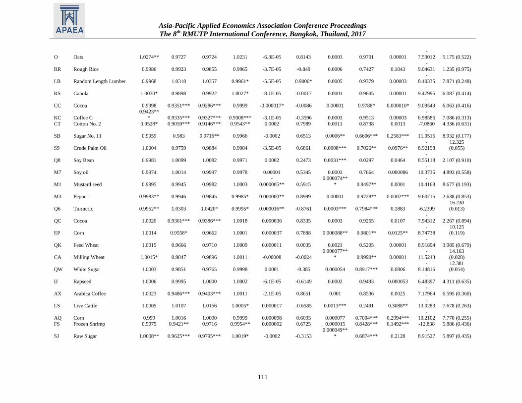
Asia-Pacific Applied Economics Association Conference Proceedings
The 8th RMUTP International Conference, Bangkok, Thailand, 2017
111
O Oats 1.0274** 0.9727 0.9724 1.0231 -6.3E-05 0.8143 0.0003 0.9701 0.00001 -
7.53012 5.175 (0.522)
RR Rough Rice 0.9986 0.9923 0.9855 0.9965 -3.7E-05 -0.849 0.0006 0.7427 0.1043
-
9.04631 1.235 (0.975)
LB Random Length Lumber 0.9968 1.0318 1.0357 0.9961* -5.5E-05 0.9000* 0.0005 0.9379 0.00003
-
8.40335 7.871 (0.248)
RS Canola 1.0030* 0.9898 0.9922 1.0027* -8.1E-05 -0.0017 0.0001 0.9605 0.00001 -
9.47995 6.087 (0.414)
CC Cocoa 0.9998 0.9351*** 0.9286*** 0.9999 -0.000017* -0.0086 0.00001 0.9788* 0.000010*
-
9.09549 6.063 (0.416)
KC Coffee C
0.9423**
* 0.9335*** 0.9327*** 0.9308*** -3.1E-05 -0.3596 0.0003 0.9513 0.00003
-
6.98585 7.086 (0.313)
CT Cotton No. 2 0.9528* 0.9059*** 0.9146*** 0.9543** 0.0002 0.7989 0.0011 0.8738 0.0013 -7.0860 4.336 (0.631)
SB Sugar No. 11 0.9959 0.983 0.9716** 0.9966 -0.0002 0.6513 0.0006** 0.6606*** 0.2583***
-
11.9515 8.932 (0.177)
S9 Crude Palm Oil 1.0004 0.9759 0.9884 0.9984 -3.5E-05 0.6861 0.0008*** 0.7026** 0.0976** -
8.92198 12.325 (0.055)
Q8 Soy Bean 0.9981 1.0099 1.0082 0.9971 0.0002 0.2473 0.0031*** 0.0297 0.0464
-
8.55118 2.107 (0.910)
M7 Soy oil 0.9974 1.0014 0.9997 0.9978 0.00001 0.5345 0.0003 0.7664 0.000086
-
10.3735 4.893 (0.558)
M1 Mustard seed 0.9995 0.9945 0.9982 1.0003
-
0.000005** 0.5915
0.000074**
* 0.9497** 0.0001
-
10.4168 8.677 (0.193)
M3 Pepper 0.9983** 0.9946 0.9845 0.9985* 0.000000** 0.8999 0.00001 0.9728** 0.0002*** -
9.60715 2.638 (0.853)
Q6 Turmeric 0.9952** 1.0303 1.0420* 0.9995*
-
0.000016** -0.8761 0.0003*** 0.7984*** 0.1883 -6.2399
16.230
(0.013)
QC Cocoa 1.0020 0.9361*** 0.9386*** 1.0018 0.000036 0.8335 0.0003 0.9265 0.0107
-
7.94312 2.267 (0.894)
EP Corn 1.0014 0.9558* 0.9662 1.0001 0.000037 0.7888 0.000088** 0.9801** 0.0125** -
8.74738 10.125 (0.119)
QK Feed Wheat 1.0015 0.9666 0.9710 1.0009 0.000011 0.0035 0.0021 0.5205 0.00001
-
8.91894 3.985 (0.679)
CA Milling Wheat 1.0015* 0.9847 0.9896 1.0011 -0.00008 -0.0024
0.000077**
* 0.9990** 0.00001
-
11.5243
14.163
(0.028)
QW White Sugar 1.0003 0.9851 0.9765 0.9998 0.0001 -0.385 0.000054 0.8917*** 0.0806 -
8.14816 12.381 (0.054)
IJ Rapseed 1.0006 0.9995 1.0000 1.0002 -6.1E-05 -0.6149 0.0002 0.9493 0.000053
-
6.48397 4.311 (0.635)
AX Arabica Coffee 1.0023 0.9486*** 0.9403*** 1.0011 -2.1E-05 0.8651 0.001 0.8536 0.0025
-
7.17964 6.595 (0.360)
LS Live Cattle 1.0005 1.0107 1.0156 1.0005* 0.000017 -0.6585 0.0013*** 0.2491 0.3088** -
13.0283 7.678 (0.263)
AQ Corn 0.999 1.0016 1.0000 0.9999 0.000098 0.6093 0.000077 0.7004*** 0.2994***
-
10.2102 7.770 (0.255) FS Frozen Shrimp 0.9975 0.9421** 0.9716 0.9954** 0.000002 0.6725 0.000015 0.8428*** 0.1492*** -12.838 5.886 (0.436)
SJ Raw Sugar 1.0008** 0.9625*** 0.9795*** 1.0019* -0.0002 -0.3153
0.000049**
* 0.6874*** 0.2128
-
8.91527 5.897 (0.435)

Asia-Pacific Applied Economics Association Conference Proceedings
The 8th RMUTP International Conference, Bangkok, Thailand, 2017
112
MW Hard Red Spring Wheat 1.0026 0.9766 0.9843 1.0031 0.000064 -0.7947 0.0044** 0.051 0.2003** -
7.67497 3.540 (0.739)
WZ White Maize 1.0039 0.9551 0.9527* 1.0037 0.0001** 0.8982 0.0072*** 0.000017 0.1533**
-
8.29453 5.838 (0.442)
YW Yellow Maize 1.0000 0.9737 0.9797 1.0000 -7E-06 0.0414 0.00001 0.000011 0.0694*
-
7.93956 5.542 (0.476)
EB Bread milling wheat 1.0040**
* 0.9784 0.9722 1.0035*** -1.8E-05 0.7764 0.0005 0.8445 0.000016 -
8.89109 8.045 (0.235)
SY Soybeans of Class SB 0.9996 0.9828 0.9847 0.9985 -2.1E-05 0.0886 0.003 0.5291 0.000012
-
8.39984 2.361 (0.884)
SU Sunflower Seed 1.0017 0.9691 0.9800** 1.0013 0.000041 0.3973 0.0004* 0.944 0.00005
-
8.06202 8.795 (0.185)
JC Corn 1.0016 1.0062 1.0033 1.0007 0 -0.4221 0.0006 0.9273 0.0002 -
9.45344 3.830 (0.700)
JS Soybean 1.0014 0.9769 1.0084 1.0006 -0.0002 0.8402 0.0021 0.8338 0.0027
-
8.65314 3.556 (0.736)
JZ Arabica Coffee
1.0012**
* 0.9010*** 0.8986 0.9995*** -0.0004 0.8992 0.01 0.2681 0.0002
-
7.85066
26.723
(0.000)
JR Raw Sugar 1.0034 1.0049 1.0075 0.9986 0.0018 -0.756 0.0006*** 0.999 0.000011 -
10.0979 2.896 (0.822)
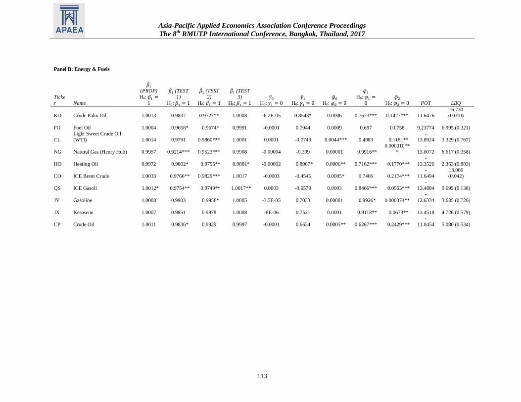
Asia-Pacific Applied Economics Association Conference Proceedings
The 8th RMUTP International Conference, Bangkok, Thailand, 2017
113
Panel B: Energy & Fuels
Ticke
r Name
�̂�1 (PROP)
H0: 𝛽1 =1
�̂�1 (TEST
1)
H0: 𝛽1 = 1
�̂�1 (TEST
2)
H0: 𝛽1 = 1
�̂�1 (TEST
3)
H0: 𝛽1 = 1
𝛾0
H0: 𝛾1 = 0
𝛾1
H0: 𝛾1 = 0
�̂�0
H0: 𝜑0 = 0
�̂�1
H0: 𝜑1 =0
�̂�2
H0: 𝜑2 = 0 POT LBQ
KO Crude Palm Oil 1.0013 0.9837 0.9727** 1.0008 -6.2E-05 0.8543* 0.0006 0.7673*** 0.1427*** -
11.6476 16.730 (0.010)
FO Fuel Oil 1.0004 0.9658* 0.9674* 0.9991 -0.0001 0.7044 0.0009 0.697 0.0758
-
9.23774 6.995 (0.321)
CL
Light Sweet Crude Oil
(WTI) 1.0014 0.9791
0.9860*** 1.0001 0.0001 -0.7743 0.0044*** 0.4083 0.1181**
-
13.8924 3.329 (0.767)
NG Natural Gas (Henry Hub) 0.9957
0.9214***
0.9523*** 0.9908 -0.00004 -0.399 0.00001 0.9916** 0.000010**
* -
13.0072 6.617 (0.358)
HO Heating Oil 0.9972 0.9802* 0.9795** 0.9881* -0.00002 0.8967* 0.0006**
0.7162*** 0.1770***
-
13.3526 2.363 (0.883)
CO ICE Brent Crude 1.0033 0.9766**
0.9829*** 1.0017 -0.0003 -0.4545 0.0005* 0.7406 0.2174***
-
11.6494
13.066
(0.042)
QS ICE Gasoil 1.0012* 0.9754** 0.9749** 1.0017** 0.0003 -0.6579 0.0003
0.8466*** 0.0963*** -
13.4884 9.695 (0.138)
JV Gasoline 1.0008 0.9903 0.9958* 1.0005 -3.5E-05 0.7033 0.00001 0.9926* 0.000074**
-
12.6334 3.635 (0.726)
JX Kerosene 1.0007 0.9851 0.9878 1.0008 -8E-06 0.7521 0.0001 0.9118** 0.0673**
-
13.4518 4.726 (0.579)
CP Crude Oil 1.0011 0.9836* 0.9929 0.9997 -0.0001 0.6634 0.0005**
0.6267*** 0.2429*** -
11.0454 5.080 (0.534)

Asia-Pacific Applied Economics Association Conference Proceedings
The 8th RMUTP International Conference, Bangkok, Thailand, 2017
114
Panel C: Industrial Materials
Ticke
r Name
�̂�1 (PROP)
H0: 𝛽1 =1
�̂�1 (TEST
1)
H0: 𝛽1 = 1
�̂�1 (TEST
2)
H0: 𝛽1 = 1
�̂�1 (TEST
3)
H0: 𝛽1 = 1
𝛾0
H0: 𝛾1 = 0
𝛾1
H0: 𝛾1 = 0
�̂�0
H0: 𝜑0 = 0
�̂�1
H0: 𝜑1 =0
�̂�2
H0: 𝜑2 = 0 POT LBQ
CU Copper Cathode 1.0007 0.9913 1.0003 1.0011* 0.000001 0.8164 0.0005 0.7369* 0.1603*** -
14.7415 4.934 (0.552)
AA Aluminum 1.0002 0.9722
0.9857*** 1.0005 0.000003 0.7253 0.000075
0.8618*** 0.0735***
-
13.4104
10.177
(0.117)
HG Copper 1.0037 0.9942 0.9991 1.0017 -2.9E-05 0.7029 0.0005*** 0.6953 0.1797***
-
12.9371 1.213 (0.976)
S4 Nickel 1.0002 0.9706 0.9887 1.0011 0.00001 -0.7461 0.000028
0.9827*** 0.000082**
* -
9.57958 7.580 (0.271)
LA Aluminium 1.0004 0.9705* 0.9729 1.0000 0.00003
-
0.8704*** 0.0001*** 0.8944* 0.0533**
-
13.0441
13.958
(0.030)
LY Aluminium Alloy 1.0003* 0.9813 0.9929 1.0003
0.000052**
* -0.3216 0.0006*** 0.0104 0.9896***
-
11.6146
10.952
(0.090)
LP Copper 1.0008 0.9942 0.9983 1.0010 -8.6E-05 0.6585 0.0002
0.8263*** 0.1188*** -
11.8638 8.298 (0.217)
LX Zinc 1.0003 0.9836 0.9962 1.0000 0.000018 -0.6255 0.000042
0.9296*** 0.0677***
-
13.2289 5.925 (0.432)
JN Rubber 1.0031 0.9889 0.9860 0.9988 0.000004 0.8637 0.000013 0.9965 0.000019
-
13.3672 6.383 (0.382)

Asia-Pacific Applied Economics Association Conference Proceedings
The 8th RMUTP International Conference, Bangkok, Thailand, 2017
115
Panel D: Precious Metals
Ticke
r Name
�̂�1 (PROP)
H0: 𝛽1 =1
�̂�1 (TEST
1)
H0: 𝛽1 = 1
�̂�1 (TEST
2)
H0: 𝛽1 = 1
�̂�1 (TEST
3)
H0: 𝛽1 = 1
𝛾0
H0: 𝛾1 = 0
𝛾1
H0: 𝛾1 = 0
�̂�0
H0: 𝜑0 = 0
�̂�1
H0: 𝜑1 =0
�̂�2
H0: 𝜑2 = 0 POT LBQ
GC Gold 1.0017** 0.9929 0.9911 1.0002 -3E-06 0.0079 0.0012*** 0.000084 0.4406* -
9.50594 3.761 (0.709)
SI Silver 1.0017 0.9700** 0.9936*** 1.0002 0.000044 0.7223 0.0018*** 0.437 0.2355
-
11.0303
10.735
(0.097)
PA Palladium 0.9978 0.9647 0.9582* 0.9973 -4.8E-05 0.1502 0.00001 0.9792 0.00001
-
9.03038 8.037 (0.235)
Z7 Gold 1.0008 0.9801 1.0012 1.0002 0.0001 -0.0447 0.0006* 0.3779*** 0.4568*** -
10.9924 8.044 (0.235)
U5 Gold 1.001 0.9789 0.9849 1.0009 0.0001 0.5817 0.00001 0.9865 0.000014
-
8.83942 4.158 (0.655)
SN Silver M
1.0025**
* 0.9963 0.9944 1.0027 -0.0002 -0.7246 0.0029*** 0.5786 0.0343***
-
8.46502 3.530 (0.740)
JG Gold 1.0009 0.9936 0.9994 0.9990 0.000013**
* 0.8493 0.001 0.3733 0.0989*** -
9.75593 3.256 (0.776)
JI Silver 0.9801 0.9873 0.9804 0.9886 -0.0002 -0.6454 0.0038 0.8245 0.00001
-
9.50134 4.072 (0.667)
JA Platinum 1.0011 0.9806 0.9753*** 1.0005 0.000007 0.4284 0.0008*** 0.3737** 0.4017***
-
8.09886 8.137 (0.228)
JM Palladium 1.0033 1.0228 1.0253 1.0015 0.000042 0.8993* 0.0007 0.8293* 0.0454*** -
9.72711 4.400 (0.623)

Asia-Pacific Applied Economics Association Conference Proceedings
The 8th RMUTP International Conference, Bangkok, Thailand, 2017
116
Table 2. Comparing Results of Market Efficiency Tests This table summarises the efficiency test results in Table 1 corresponding to the proposed market efficiency test (PROP) and TEST1-TEST3.
In Table 1, the PROP identifies a total of 68 commodities as efficient and 11 commodities as inefficient in the entire sample and they are
indicated in the two rows of this Table. The number of commodities identified by TEST1-3 as efficient and inefficient in Table 1 are expressed
in this Table as a percentage of the number classified as efficient (i.e., 68) and inefficient (i.e., 11) by PROP for comparison purpose.
TEST1 TEST2 TEST3
Inefficient Efficient Inefficient Efficient Inefficient Efficient
Count % Count % Count % Count % Count % Count %
PROP Inefficient (11) 3 27.3% 8 72.7% 3 27.3% 8 72.7% 5 45.5% 6 54.5%
Efficient (68) 9 13.2% 59 86.8% 17 25.0% 51 75.0% 5 7.4% 63 92.6%

Asia-Pacific Applied Economics Association Conference Proceedings
The 8th RMUTP International Conference, Bangkok, Thailand, 2017
117
Table 3. Summary of Estimated Risk Premiums by PROP This table summarises the estimated annualized risk premiums of the 79 commodities in the sample using PROP during the sample period 2000 to 2014. Average
and the volatility of the annualized time-varying risk premiums of each commodity are reported in Panel A and B respectively. Results are summarized for the
full sample as well as by market sectors. The last column presents the Stem-and-Leaf plots of average risk premiums and the volatility of each commodity for the
full sample period 2000-2014.
Panel A: Analysis of average annualized risk premiums
Annualized Risk Premium Stem-and-Leaf Plot for the Full Sample
Full Sample
Agricultural
& Livestock
Energy &
Fuels
Industrial
Materials
Precious
Metals Frequency Stem & Leaf
Mean 0.422 0.290 0.998 0.535 0.475 2.00 Extremes (=<-1.9)
95% Confidence Interval for
Mean (0.115,0.729)
(-0.105,
0.686) (-0.396,2.392)
(-0.392,
1.461) (-0.087,1.038)
2.00 -1 . 12
7.00 -0 . 5577799
Median 0.179 0.106 0.470 0.067 0.347 19.00 -0 . 0000000112222233344
Std. Deviation 1.371 1.407 1.814 1.206 0.786 25.00 0 . 0000000111222223333444444
Minimum -4.012 -4.012 -0.235 -0.585 -0.181 9.00 0 . 555667899
Maximum 5.611 5.018 5.611 3.320 2.574 6.00 1 . 022244
Skewness 1.251 0.824 2.520 1.796 2.480 2.00 1 . 58
Kurtosis 4.796 3.965 6.759 3.461 6.949 7.00 Extremes (>=2.5)
Quartile 1 -0.235 -0.337 -0.021 -0.192 -0.006 Stem width: 1.00
Quartile 3 0.695 0.669 1.236 1.108 0.550 Each leaf: 1 case(s)
% Positive avg. risk premiums 62% 55% 67% 78% 80%
Panel B: Analysis of volatility of annualized risk premiums
Standard Deviation of Annualized Risk Premiums Stem-and-Leaf Plot for the Full Sample
Full Sample
Agricultural
& Livestock
Energy &
Fuels
Industrial
Materials
Precious
Metals Frequency Stem & Leaf
Mean 6.817 6.860 7.577 4.495 7.999 11.00 0 . 00000000111
95% Confidence Interval for
Mean (5.791,7.842) (5.620,8.100) (4.338,10.816) (1.462,7.529) (3.678,12.321)
10.00 0 . 2222223333
17.00 0 . 44444455555555555
Median 6.160 6.623 6.404 4.055 5.975 16.00 0 . 6666666666777777
Std. Deviation 4.578 4.408 4.214 3.946 6.041 9.00 0 . 888888889
Minimum < 0.001 0.001 3.863 < 0.001 0.265 5.00 1 . 00111
Maximum 19.635 19.635 18.121 11.362 19.204 6.00 1 . 223333
Skewness 0.838 0.681 2.341 0.445 0.877 5.00 Extremes (>=17)
Kurtosis 0.616 0.352 6.152 -0.797 0.044
Quartile 1 3.864 3.695 5.285 0.516 3.921 Stem width: 10.00
Quartile 3 8.829 8.931 6.404 7.578 11.982 Each leaf: 1 case(s)

Asia-Pacific Applied Economics Association Conference Proceedings
The 8th RMUTP International Conference, Bangkok, Thailand, 2017
118
Table 4. Market Efficiency, Risk Premiums and Trading Volumes during pre- and post-GFC Periods This table compares market efficiency, risk premiums estimated from PROP, and average volumes during pre- and post-GFC periods corresponding to the sample of 79
futures traded worldwide. The first and second columns present Bloomberg ticker and name of the contract of each futures. Third and fourth columns illustrate the estimated
value of 𝛽1 in equation (4) and market efficiency test results using PROP for during pre- and post-GFC periods. Fifth and sixth columns present parameter estimates
corresponding to the autoregressive coefficient of the risk premium specification in equation (4). All parameters are tested for significance using the LLR test statistic in
equation (5).Seventh and eighth columns present averages of estimated annualized risk premiums for pre- and post-GFC periods while ninth and tenth columns present
standard deviation of estimated annualized risk premiums. Eleventh and twelfth columns present average daily trading volumes of each futures during pre- and post-GFC
periods. ***, **, and * denote significance at 1%, 5%, and 10% respectively. Panels A-D summarize results by market sectors while Panel E compares results between
pre-GFC ( January 2000-August 2008) and post-GFC (September 2008-December 2014) periods. The inefficient markets where the null hypothesis 𝐻0: 𝛽1 = 1 is rejected
are marked with an asterisks *.
(1) (2) (3) (4) (5) (6) (7) (8) (9) (10) (11) (12)
Panel A: Agricultural & Livestock
Tic
ker Name
�̂�1 (Pre-
GFC) H0:
𝛽1 = 1
�̂�1 (Post-
GFC) H0:
𝛽1 = 1
𝛾1 (Pre-
GFC) H0:
𝛾1 = 0
𝛾1 (Post-
GFC) H0:
𝛾1 = 0
Average Risk
Premium
(Pre-GFC)
Average Risk
Premium
(Post-GFC)
Stdev of Risk
Premium
(Pre-GFC)
Stdev of Risk
Premium
(Post-GFC)
Average Volume
(Pre-GFC)
Average Volume
(Post-GFC)
AC Corn
0.9998
*** 0.9989
0.2099
** 0.5475 -0.0328 0.7606 0.020 3.581 9561.35 2331.97
AK No.1 Soybeans 1.0026* 1.0002 0.8998 0.5078 -2.9190 -0.2156 13.866 8.451 15618.71 718.95
AE Soybean Meal
1.0023
** 1.0025
-
0.9000
-
0.6234 2.5068 -6.4204 11.080 4.176 7794.96 7920.18
C Corn 0.9918 1.0053
-
0.1714 0.6025 0.2514 0.2584 7.682 3.228 51834.12 125570.88
S Soybeans 1.0094* 1.0030 0.6006
-0.8824 -0.8318 14.7986 3.917 18.103 34451.10 81869.92
BO Soybean Oil 0.9925 1.0151 0.5872 0.7228 -0.8399 0.8655 3.685 5.648 13905.77 38248.24
SM Soybean Meal
1.0040
*
1.0050
** 0.7026
-0.8999
* -0.4340 0.7166 5.166 19.600 13872.48 28921.55
W Wheat 1.0122 1.0018 -
0.5748 -
0.0766 -0.4254 1.6441 0.031 2.343 21369.56 48514.32
YP
Mini-sized
Wheat 1.0264 1.0034 0.6521 0.7017 9.8433 0.1453 30.990 0.325 97.88 309.24
LC Live Cattle 0.9677 1.0287
-
0.8358
-
0.8187 -0.0734 -1.4337 12.623 8.332 9213.38 17674.16
LH Lean Hogs 0.9298* 0.9408
-0.9000
-0.8963 -8.4833 -0.4691 13.640 13.592 4638.43 10322.54
FC Feeder Cattle 0.9582
1.0162
* 0.5392 0.4971 -0.1185 -0.0215 5.377 7.161 881.98 1277.76 DA Class III Milk 0.9986 0.9998 0.2306 0.6703 0.2689 5.5723 1.737 5.875 58.20 165.03
KV Class IV Milk 1.0007 1.0008
0.6640
* 0.7860 -1.1438 -0.8457 5.923 9.926 0.34 1.07

Asia-Pacific Applied Economics Association Conference Proceedings
The 8th RMUTP International Conference, Bangkok, Thailand, 2017
119
(1) (2) (3) (4) (5) (6) (7) (8) (9) (10) (11) (12)
Panel A: Agricultural & Livestock
Tic
ker Name
�̂�1 (Pre-
GFC) H0:
𝛽1 = 1
�̂�1 (Post-
GFC) H0:
𝛽1 = 1
𝛾1 (Pre-
GFC) H0:
𝛾1 = 0
𝛾1 (Post-
GFC) H0:
𝛾1 = 0
Average Risk
Premium
(Pre-GFC)
Average Risk
Premium
(Post-GFC)
Stdev of Risk
Premium
(Pre-GFC)
Stdev of Risk
Premium
(Post-GFC)
Average Volume
(Pre-GFC)
Average Volume
(Post-GFC)
LE
Nonfat Dry
Milk 0.9848
1.0122
**
0.6663
** 0.8423 -1.0937 1.4024 5.351 10.507 0.07 3.74
O Oats 1.0522** 1.0180 0.8344
-0.0681 0.8663 0.7803 1.372 1.544 671.04 627.55
RR Rough Rice 1.0063 0.9933 0.6910 0.5973 -0.0573 0.6755 0.070 8.032 280.90 652.96
LB Random Length
Lumber 0.9965 1.0012 0.8826 -
0.2228 0.5415 -0.8570 10.327 1.288 577.82 524.58
RS Canola
1.0033
**
1.0030
*
-
0.4805 0.0009 -0.5596 -4.4141 4.670 0.883 4416.73 8870.11
CC Cocoa 1.0015 0.9994
-
0.5823
-
0.5448 -0.0161 -2.5653 2.090 0.062 3420.44 6617.97
KC Coffee C ® 0.9118*** 0.9693
-0.6135
-0.7226 -0.2979 1.1374 24.968 5.393 5107.96 6101.01
CT Cotton No. 2
0.9662
*
0.8749
** 0.7749 0.8996 0.8464 -0.4804 6.308 13.823 7425.65 8989.05
SB Sugar No. 11
0.9950
* 0.9979 0.4245 0.8999 -0.6867 0.1293 12.927 6.567 25096.64 49592.45
S9
Crude Palm
Oil 0.9943 1.0012 0.4482 0.7955 0.3819 -5.3721 3.785 10.285 14.80 445.39
Q8 Soy Bean 1.0005 1.0002 0.6420 -
0.6991 -6.2872 -0.7073 23.761 14.415 14377.16 69222.89
M7 Soy oil
0.9949
** 0.9979
0.8984
**
-
0.1551 2.6190 -25.3810 11.217 3.267 16157.98 72473.49
M1 Mustard seed 0.9983 0.9998
-
0.2429 0.1402 0.4554 -0.0794 9.325 3.841 17697.45 64193.16
M3 Pepper 0.9979 0.9969 0.8767 0.0191 -0.0187 -1.7944 0.298 0.040 4269.00 3811.74
Q6 Turmeric
0.9914
*** 1.0010
-
0.8036 0.8952 3.4333 -2.1787 17.110 14.454 12550.00 13243.22
QC Cocoa 1.0038 1.0021 0.6456
-0.9000
** -0.7914 0.2336 2.940 18.145 2742.03 4899.26
EP Corn 1.0034 0.9968 0.6708 0.9000 -0.9136 0.0882 3.711 16.680 177.50 702.28
QK Feed Wheat 1.0016 0.9995
-
0.0521
-
0.5377 -0.0610 -0.0314 1.477 0.382 103.81 157.08
CA Milling Wheat 1.0013 1.0010 0.4104 0.0098 0.6537 0.0045 2.079 1.042 517.42 12818.29 Q
W White Sugar 1.0008 1.0000
-
0.6519
-
0.8999 -1.5898 -4.3671 5.949 17.061 3017.00 3560.75
IJ Rapseed 0.9998 1.0027 0.7533 0.5421 -1.3269 -4.5791 5.099 0.663 367.83 2812.82
AX
Arabica
Coffee
1.0059
* 0.9984
-
0.8211
-
0.8846 -0.3093 5.1937 5.017 5.374 634.39 607.12
LS Live Cattle 0.9994 1.0014 -
0.6288 0.0913 0.3590 0.2340 2.186 2.945 42.33 1801.53

Asia-Pacific Applied Economics Association Conference Proceedings
The 8th RMUTP International Conference, Bangkok, Thailand, 2017
120
(1) (2) (3) (4) (5) (6) (7) (8) (9) (10) (11) (12)
Panel A: Agricultural & Livestock
Tic
ker Name
�̂�1 (Pre-
GFC) H0:
𝛽1 = 1
�̂�1 (Post-
GFC) H0:
𝛽1 = 1
𝛾1 (Pre-
GFC) H0:
𝛾1 = 0
𝛾1 (Post-
GFC) H0:
𝛾1 = 0
Average Risk
Premium
(Pre-GFC)
Average Risk
Premium
(Post-GFC)
Stdev of Risk
Premium
(Pre-GFC)
Stdev of Risk
Premium
(Post-GFC)
Average Volume
(Pre-GFC)
Average Volume
(Post-GFC) AQ Corn 1.0009 0.9986 0.0235 0.4600 1.1450 0.0457 1.542 2.584 76.69 6.41
FS Frozen Shrimp
0.9932
* 0.9996
-
0.3090 0.5998 0.3517 5.6118 3.556 6.668 153.39 2.76
SJ Raw Sugar 1.0022 1.0007
-
0.8441
0.7746
* -0.3976 0.5680 3.456 8.893 9.69 2.86 M
W Hard Red Spring
Wheat 1.0047 0.9998
-
0.8422 0.1324 0.9293 -0.4295 2.278 0.370 2091.29 2207.21
WZ White Maize 1.0066*** 1.0045 0.6973 0.6968 -4.9046 0.5959 21.281 5.449 1548.44 1842.64
Y
W Yellow Maize 1.0000 1.0001
-
0.5508 0.5525 -0.0002 2.1622 0.001 0.113 72329.93 125570.88
EB
Bread milling
wheat
1.0046
** 1.0038 0.7521
-
0.7527 0.0519 0.4371 9.460 7.364 454.75 1619.82
SY Soybeans of Class SB
1.0023*** 0.9988 0.8998
-0.2686 0.9068 0.2268 0.098 1.201 34.83 553.29
SU Sunflower Seed 1.0028 1.0001
-0.4002
-0.8633 -3.4422 -0.0762 13.058 0.262 104.04 398.50
JC Corn 1.0038 0.9996 0.3232
-
0.6052 0.1410 -0.5247 0.724 2.377 401.40 79.30
JS Soybean 1.0021
1.0040
***
-
0.0121 0.8198 -0.3076 0.0765 4.344 0.878 110.18 71.53
JZ
Arabica
Coffee
1.0082
**
0.9908
***
-
0.8999
0.8986
*** -2.9811 0.0465 21.251 40.638 105.64 7.03
JR Raw Sugar 1.0004 1.0000 -
0.8996 -
0.7051 3.5979 0.2644 23.708 5.772 75.74 14.21
Panel B: Energy & Fuels
Tic
ker Name
�̂�1 (Pre-GFC)
H0:
𝛽1 = 1
�̂�1 (Post-GFC)
H0:
𝛽1 = 1
𝛾1 (Pre-GFC)
H0:
𝛾1 = 0
𝛾1 (Post-GFC)
H0:
𝛾1 = 0
Average Risk
Premium (Pre-GFC)
Average Risk
Premium
(Post-GFC)
Stdev of Risk
Premium
(Pre-GFC)
Stdev of Risk
Premium
(Post-GFC)
Average Volume
(Pre-GFC)
Average Volume
(Post-GFC)
FO Fuel Oil 1.0025 0.9994 0.6003 0.3453 -0.3947 -0.5827 3.553 9.575 3006.31 12816.97
CL
Crude Oil
(WTI) 1.0035 1.0006
-
0.5147
-
0.8495 -0.0392 -1.3900 3.518 13.286 114045.40 251817.25
NG Natural Gas (Henry Hub) 0.9999 0.9927 0.7388 0.8545 -0.2425 -0.5310 0.978 3.445 38698.17 106352.49
HO Heating Oil 0.9933 0.9986
0.8988
** 0.6340 9.4872 -1.1770 12.992 4.863 24786.87 51981.68

Asia-Pacific Applied Economics Association Conference Proceedings
The 8th RMUTP International Conference, Bangkok, Thailand, 2017
121
(1) (2) (3) (4) (5) (6) (7) (8) (9) (10) (11) (12)
Panel A: Agricultural & Livestock
Tic
ker Name
�̂�1 (Pre-
GFC) H0:
𝛽1 = 1
�̂�1 (Post-
GFC) H0:
𝛽1 = 1
𝛾1 (Pre-
GFC) H0:
𝛾1 = 0
𝛾1 (Post-
GFC) H0:
𝛾1 = 0
Average Risk
Premium
(Pre-GFC)
Average Risk
Premium
(Post-GFC)
Stdev of Risk
Premium
(Pre-GFC)
Stdev of Risk
Premium
(Post-GFC)
Average Volume
(Pre-GFC)
Average Volume
(Post-GFC)
CO
ICE Brent
Crude 1.0070
1.0018
**
-
0.4132
-
0.4445 0.6954 1.0308 3.961 12.071 55481.46 172056.62
QS ICE Gasoil 1.0040 1.0001 -
0.8422 0.1647 0.7077 0.6204 10.946 2.812 20377.14 58987.66
JV Gasoline 1.0012
1.0021** 0.3191 0.8991 -0.1502 0.6616 2.134 10.652 777.31 285.51
JX Kerosene 1.0025*
1.0014** 0.4430
-0.7624 -0.0849 -0.1791 1.583 7.450 612.62 356.29
CP Crude Oil 1.0022 1.0006 0.7765 0.4903 0.0806 0.0781 1.646 4.458 117.08 67.53

Asia-Pacific Applied Economics Association Conference Proceedings
The 8th RMUTP International Conference, Bangkok, Thailand, 2017
122
(1) (2) (3) (4) (5) (6) (7) (8) (9) (10) (11) (12)
Panel C: Industrial Materials
Tic
ker Name
�̂�1 (Pre-
GFC)
H0:
𝛽1 = 1
�̂�1 (Post-
GFC)
H0:
𝛽1 = 1
𝛾1 (Pre-
GFC)
H0:
𝛾1 = 0
𝛾1 (Post-
GFC)
H0:
𝛾1 = 0
Average Risk Premium
(Pre-GFC)
Average Risk Premium
(Post-GFC)
Stdev of Risk Premium
(Pre-GFC)
Stdev of Risk Premium
(Post-GFC)
Average Volume
(Pre-GFC)
Average Volume
(Post-GFC)
CU Copper Cathode 1.0012 1.0004
0.8744** 0.7268 1.7873 -0.4047 10.437 1.588 2841.28 10184.66
AA Aluminum
1.0001
** 0.9996
0.4908
** 0.1857 1.2006 0.0576 4.950 3.929 1560.23 3744.63
HG Copper 1.0103 0.9973
0.7317
** -0.6241 2.2705 -0.0146 6.959 4.359 6467.63 22674.96
S4 Nickel 1.0065 0.9989 0.7901 0.2305 3.7353 -0.0269 6.920 0.018 3884.43 37947.64
LA Aluminium 1.0004 1.0002
-
0.7528 -0.7412 -0.5452 0.3124 6.414 10.064 3649.25 23913.00
LY
Aluminium
Alloy 1.0006
1.0008
*** 0.5029
-0.8841
** -1.0483 -0.8308 3.330 10.143 13.19 201.97
LP Copper 1.0011 1.0006 0.7489 0.5196 0.1032 -0.2872 7.845 3.713 1851.89 9383.14 LX Zinc 0.9993 1.0005 0.8245 -0.8952 0.5946 -1.1018 10.075 16.503 1238.06 6197.45
JN Rubber 1.0120 1.0024 0.8994 0.8841 3.5287 -1.0786 4.156 10.356 416.69 79.67
Panel D: Precious Metals
Ticker Name
�̂�1 (Pre-
GFC) H0:
𝛽1 = 1
�̂�1 (Post-
GFC) H0:
𝛽1 = 1
𝛾1 (Pre-
GFC) H0:
𝛾1 = 0
𝛾1 (Post-
GFC) H0:
𝛾1 = 0
Average Risk Premium (Pre-GFC)
Average Risk
Premium (Post-GFC)
Stdev of Risk
Premium (Pre-GFC)
Stdev of Risk
Premium (Post-GFC)
Average Volume (Pre-GFC)
Average Volume (Post-GFC)
GC Gold 1.0015 1.0009 -0.4137 -0.8730 0.6334 -1.7954 3.704 12.274 29270.57 69395.57
SI Silver 1.0080* 0.9962
-
0.1081*** -0.8899 0.0341 19.2679 5.942 8.696 9845.13 21496.61
PA
Palladi
um 0.9990 0.9977 -0.9000 0.7870 2.6162 8.6087 11.444 10.659 450.69 2226.30 Z7 Gold 1.0005 1.0003 0.0014 -0.6990 0.6558 5.6302 3.419 5.597 64250.08 104903.28
U5 Gold 1.0013 1.0008 -0.5703 -0.5633 -0.2000 2.5024 3.138 4.577 356144.18 33657.13
SN Silver M 1.0035 1.0036 0.6902 -0.0152 -1.8001 2.1528 3.302 1.922 10910.77 78730.04
JG Gold
1.0020
* 1.0029 -0.0510 0.6932 1.0235 2.4285 4.082 10.988 655.12 290.66 JI Silver 0.9794 0.9516 0.7848 0.8896 16.5195 4.3960 4.398 33.460 700127.43 2297785.95
JA
Platinu
m 1.0028 0.9984 -0.6056 0.7067 0.6820 0.2862 1.547 19.364 472.20 67.28
JM
Palladi
um 0.9968 1.0059 -0.0201 0.8286 0.2244 -0.2171 6.926 17.404 44.88 5.33

Asia-Pacific Applied Economics Association Conference Proceedings
The 8th RMUTP International Conference, Bangkok, Thailand, 2017
123
Panel E: Comparison between two sub periods Post-GFC Total Wilcoxon Signed Ranks Tests for Significant Differences
Inefficient Efficient H0: There is no difference in averages
Market efficiency at 5% level Mean Test Statistic P-value
Pre-GFC
Inefficient Count 1 12 13 Average Risk Premium Pre-GFC 0.385 -0.264 0.792
% of Total 1.3% 15.2% 16.5% Post-GFC 0.253
Efficient Count 8 58 66 Stdev of Risk Premium Pre-GFC 6.747 -1.276 0.202
% of Total 10.1% 73.4% 83.5% Post-GFC 7.822
Total Count 9 70 79 Average Trading Volume Pre-GFC 23200.5
-5.449 < 0.001 % of Total 11.4% 88.6% 100.0% Post-GFC 53462.7

Asia-Pacific Applied Economics Association Conference Proceedings
The 8th RMUTP International Conference, Bangkok, Thailand, 2017
124
Table 5. Simulation Results: The size test results corresponding to an efficient market i.e., 𝛃𝟏 = 𝟏 This table compares the performance of the proposed test PROP and TEST3 with the conventional tests TEST1-2 discussed in section 2.1. TEST1-3 are
derived by relaxing the time varying risk premium and heteroscedasticity assumptions in PROP. TEST1-2 represent conventional market efficiency tests
and TEST3 is a simplified version of PROP. Here, the time-varying property of the risk premium is simulated by varying 𝛾1of equation (4b) in column
one of the Table. The degree of the conditional heteroscedasticity of spot prices is introduced by varying the parameters 𝜑1 and 𝜑2 of equation (4e) in
different panels. Results are based on 5000 simulation runs from an efficient market, 𝛽1 = 1, using the DGP in equations (4a)-(4e). The RMSE is the
root mean square of residuals. N is the number of contracts (sample size). 𝛾1 % of acceptance of efficient market hypothesis at 5% Level Mean (Stdev) of �̂�1 Residual [휀�̂�(𝑡𝑖)] RMSE
(𝜑1 = 0.2)
(𝜑2 = 0.6) N TEST1 TEST2 TEST3 PROP TEST1 TEST2 TEST3 PROP TEST1 TEST2 TEST3 PROP
0 30 65.50 45.42 90.04 82.86 0.900 (0.074) 0.907 (0.101) 0.997 (0.092) 1.001 (0.005) 0.0520 0.0525 0.0500 0.0543 0 60 65.04 51.52 93.26 91.16 0.949 (0.037) 0.957 (0.051) 1.001 (0.004) 1.001 (0.003) 0.0562 0.0567 0.0549 0.0564
0 120 67.24 58.52 93.16 93.74 0.975 (0.019) 0.982 (0.023) 1.001 (0.003) 1.001 (0.002) 0.0602 0.0605 0.0586 0.0597
0 240 66.78 64.86 93.02 95.32 0.987 (0.010) 0.992 (0.010) 1.001 (0.002) 1.001 (0.002) 0.0629 0.0631 0.0606 0.0618 0 480 66.94 71.16 89.68 95.94 0.994 (0.005) 0.996 (0.004) 1.000 (0.002) 1.000 (0.002) 0.0649 0.0651 0.0620 0.0637
0.5 30 64.40 45.26 90.36 83.32 0.901 (0.074) 0.909 (0.099) 0.995 (0.226) 1.001 (0.005) 0.0519 0.0524 0.0499 0.0538
0.5 60 67.34 52.34 93.26 91.10 0.947 (0.039) 0.957 (0.054) 1.001 (0.003) 1.001 (0.003) 0.0569 0.0572 0.0553 0.0573 0.5 120 66.46 57.76 91.70 93.80 0.974 (0.019) 0.981 (0.023) 1.001 (0.003) 1.001 (0.002) 0.0600 0.0603 0.0581 0.0593
0.5 240 66.60 63.58 91.24 95.08 0.987 (0.009) 0.992 (0.010) 1.001 (0.002) 1.001 (0.002) 0.0629 0.0631 0.0606 0.0619
0.5 480 66.62 71.36 86.96 94.58 0.994 (0.005) 0.996 (0.004) 1.001 (0.002) 1.001 (0.002) 0.0650 0.0652 0.0621 0.0638 0.7 30 64.90 44.28 89.66 82.36 0.898 (0.076) 0.906 (0.105) 0.998 (0.137) 1.001 (0.005) 0.0513 0.0520 0.0492 0.0531
0.7 60 65.56 52.32 91.22 89.66 0.950 (0.038) 0.956 (0.057) 1.001 (0.006) 1.001 (0.003) 0.0570 0.0574 0.0552 0.0571
0.7 120 65.82 57.38 90.68 92.90 0.974 (0.019) 0.981 (0.025) 1.001 (0.003) 1.001 (0.002) 0.0604 0.0608 0.0586 0.0600 0.7 240 66.10 65.64 86.28 93.02 0.987 (0.010) 0.992 (0.010) 1.001 (0.002) 1.001 (0.002) 0.0630 0.0633 0.0607 0.0620
0.7 480 68.88 71.98 78.76 91.58 0.994 (0.005) 0.996 (0.004) 1.001 (0.002) 1.001 (0.002) 0.0649 0.0651 0.0622 0.0636
(𝜑1 = 0.6)
(𝜑2 = 0.2) N TEST1 TEST2 TEST3 PROP TEST1 TEST2 TEST3 PROP TEST1 TEST2 TEST3 PROP
0 30 67.06 47.84 90.34 89.50 0.899 (0.072) 0.906 (0.083) 1.000 (0.029) 1.001 (0.011) 0.0616 0.0621 0.0605 0.0632
0 60 67.72 50.28 92.92 94.56 0.948 (0.037) 0.956 (0.040) 1.001 (0.003) 1.001 (0.003) 0.0655 0.0657 0.0645 0.0655 0 120 68.50 54.02 93.90 95.26 0.974 (0.018) 0.978 (0.020) 1.001 (0.002) 1.001 (0.002) 0.0677 0.0679 0.0666 0.0672
0 240 69.02 59.70 93.50 95.34 0.987 (0.009) 0.989 (0.010) 1.001 (0.002) 1.001 (0.002) 0.0688 0.0688 0.0673 0.0679
0 480 68.82 65.00 91.56 95.50 0.994 (0.005) 0.994 (0.005) 1.000 (0.002) 1.000 (0.002) 0.0698 0.0698 0.0677 0.0685 0.5 30 67.58 47.50 89.78 89.70 0.899 (0.074) 0.909 (0.083) 0.999 (0.053) 1.001 (0.005) 0.0613 0.0618 0.0599 0.0629
0.5 60 68.24 51.24 92.86 94.18 0.948 (0.036) 0.955 (0.041) 1.001 (0.003) 1.001 (0.003) 0.0655 0.0657 0.0645 0.0655
0.5 120 69.54 54.48 92.60 94.68 0.975 (0.019) 0.979 (0.020) 1.001 (0.002) 1.001 (0.002) 0.0677 0.0678 0.0665 0.0671 0.5 240 68.58 58.78 91.58 94.70 0.987 (0.009) 0.989 (0.009) 1.001 (0.002) 1.001 (0.002) 0.0692 0.0693 0.0676 0.0682
0.5 480 68.86 65.10 88.74 94.58 0.994 (0.005) 0.994 (0.005) 1.001 (0.002) 1.001 (0.002) 0.0698 0.0699 0.0678 0.0685
0.7 30 67.58 47.50 89.78 89.70 0.899 (0.074) 0.909 (0.083) 0.999 (0.053) 1.001 (0.005) 0.0613 0.0618 0.0599 0.0629 0.7 60 68.24 51.24 92.86 94.18 0.948 (0.036) 0.955 (0.041) 1.001 (0.003) 1.001 (0.003) 0.0655 0.0657 0.0645 0.0655
0.7 120 69.08 54.64 90.16 93.60 0.974 (0.019) 0.978 (0.020) 1.001 (0.002) 1.001 (0.002) 0.0676 0.0677 0.0665 0.0671
0.7 240 68.28 60.12 88.22 93.44 0.987 (0.009) 0.989 (0.010) 1.001 (0.002) 1.001 (0.002) 0.0689 0.0689 0.0673 0.0678 0.7 480 69.06 66.38 81.58 91.68 0.994 (0.005) 0.994 (0.005) 1.001 (0.002) 1.001 (0.002) 0.0698 0.0698 0.0678 0.0685

Asia-Pacific Applied Economics Association Conference Proceedings
The 8th RMUTP International Conference, Bangkok, Thailand, 2017
125
Table 5 contd. (𝜑1 → 0)
(𝜑2 → 0) N TEST1 TEST2 TEST3 PROP TEST1 TEST2 TEST3 PROP TEST1 TEST2 TEST3 PROP
0 30 70.38 46.08 92.80 91.04 0.897 (0.071) 0.911 (0.073) 1.000 (0.088) 1.000 (0.002) 0.0293 0.0294 0.0276 0.0283
0 60 69.54 49.66 94.02 96.80 0.948 (0.036) 0.954 (0.037) 1.000 (0.001) 1.000 (0.001) 0.0305 0.0306 0.0282 0.0285
0 120 69.42 52.92 93.32 96.36 0.974 (0.018) 0.977 (0.018) 1.000 (0.001) 1.000 (0.001) 0.0311 0.0311 0.0282 0.0285
0 240 69.96 56.36 91.58 94.68 0.987 (0.009) 0.988 (0.009) 1.000 (0.001) 1.000 (0.001) 0.0314 0.0314 0.0283 0.0284
0 480 70.38 56.68 88.52 91.50 0.993 (0.005) 0.994 (0.005) 1.000 (0.000) 1.000 (0.001) 0.0315 0.0315 0.0283 0.0283
0.5 30 68.32 45.32 92.16 90.34 0.898 (0.072) 0.910 (0.077) 0.998 (0.151) 1.000 (0.003) 0.0292 0.0294 0.0276 0.0283
0.5 60 69.12 49.18 93.04 96.24 0.947 (0.036) 0.954 (0.037) 1.000 (0.001) 1.001 (0.001) 0.0304 0.0305 0.0283 0.0285
0.5 120 68.80 53.18 89.56 94.68 0.973 (0.018) 0.976 (0.019) 1.000 (0.001) 1.001 (0.001) 0.0310 0.0310 0.0282 0.0284
0.5 240 69.00 55.68 85.10 91.44 0.987 (0.009) 0.988 (0.009) 1.000 (0.001) 1.001 (0.001) 0.0314 0.0314 0.0282 0.0284
0.5 480 69.16 55.88 74.36 82.48 0.993 (0.005) 0.994 (0.005) 1.000 (0.000) 1.000 (0.000) 0.0315 0.0315 0.0283 0.0284
0.7 30 68.20 43.96 89.92 88.76 0.900 (0.071) 0.912 (0.074) 0.995 (0.356) 1.001 (0.013) 0.0292 0.0294 0.0276 0.0284
0.7 60 68.54 49.16 88.54 93.78 0.947 (0.036) 0.954 (0.038) 1.001 (0.001) 1.001 (0.001) 0.0305 0.0306 0.0282 0.0285
0.7 120 69.00 53.76 83.20 90.78 0.974 (0.018) 0.976 (0.018) 1.001 (0.001) 1.001 (0.001) 0.0311 0.0311 0.0282 0.0285
0.7 240 70.84 55.86 70.90 82.46 0.987 (0.009) 0.988 (0.009) 1.001 (0.000) 1.001 (0.001) 0.0314 0.0314 0.0283 0.0285
0.7 480 61.36 49.30 41.46 55.44 0.993 (0.005) 0.994 (0.004) 1.001 (0.000) 1.001 (0.001) 0.0315 0.0315 0.0283 0.0284

Asia-Pacific Applied Economics Association Conference Proceedings
The 8th RMUTP International Conference, Bangkok, Thailand, 2017
126
Table 6. Simulation Results: The power test results corresponding to an inefficient market, 𝛃𝟏 ≠ 𝟏 This table compares the power of the proposed test PROP with the three approaches TEST1-3. The simulated dataset is obtained by setting the value of 𝛽1in
equation (4a) around unity i.e., 𝛽1 = 0.9, 0.99, 1.01, 1.1 to simulate inefficient markets. The degree of heteroscedasticity of pricess is modelled by varying the
parameters 𝜑1 and 𝜑2 in equation (4e). Results are based on 5000 simulation runs using the DGP in equations (4a)-(4e) when 𝛾1 = 0.5
𝛽1 % of acceptance of efficient market hypothesis at 5% Level Mean (Std.dev) of �̂�1 Residual [휀�̂�(𝑡𝑖)] RMSE
(𝜑1 = 0.6)
(𝜑2 = 0.2) N TEST1 TEST2 TEST3 PROP TEST1 TEST2 TEST3 PROP TEST1 TEST2 TEST3 PROP
0.9 30 10.76 7.48 0.12 0.28 0.746 (0.124) 0.747 (0.127) 0.901 (0.017) 0.895 (0.051) 0.0557 0.0561 0.0545 0.0569
0.9 60 0.64 2.56 0.02 0.02 0.819 (0.067) 0.822 (0.067) 0.901 (0.003) 0.900 (0.018) 0.0589 0.0591 0.0579 0.0588 0.9 120 0.02 0.86 0.00 0.00 0.860 (0.034) 0.862 (0.034) 0.901 (0.002) 0.901 (0.003) 0.0611 0.0612 0.0598 0.0603
0.9 240 0.00 0.48 0.00 0.00 0.880 (0.018) 0.882 (0.017) 0.901 (0.004) 0.901 (0.002) 0.0623 0.0623 0.0606 0.061
0.9 480 0.00 0.22 0.00 0.00 0.890 (0.009) 0.891 (0.008) 0.900 (0.002) 0.900 (0.002) 0.0628 0.0629 0.0607 0.0613 0.99 30 62.88 42.94 47.62 63.78 0.819 (0.140) 0.820 (0.143) 0.991 (0.024) 0.980 (0.071) 0.0609 0.0614 0.0598 0.0631
0.99 60 58.70 39.30 27.38 43.12 0.903 (0.073) 0.905 (0.073) 0.991 (0.003) 0.990 (0.017) 0.0650 0.0652 0.0641 0.0651
0.99 120 46.24 30.78 13.78 23.82 0.945 (0.039) 0.947 (0.038) 0.991 (0.003) 0.991 (0.004) 0.0671 0.0672 0.0659 0.0665 0.99 240 20.88 16.16 7.70 12.58 0.968 (0.019) 0.969 (0.019) 0.991 (0.002) 0.991 (0.002) 0.0683 0.0684 0.0668 0.0672
0.99 480 1.86 3.26 2.26 4.22 0.979 (0.010) 0.980 (0.009) 0.991 (0.003) 0.991 (0.002) 0.0691 0.0692 0.0671 0.0678
1.01 30 70.34 48.58 38.82 58.16 0.838 (0.140) 0.839 (0.142) 1.010 (0.054) 1.000 (0.074) 0.0623 0.0629 0.0611 0.0643 1.01 60 75.10 57.72 15.38 33.72 0.920 (0.076) 0.922 (0.076) 1.010 (0.064) 1.010 (0.023) 0.0659 0.0662 0.0651 0.0663
1.01 120 80.20 65.70 7.42 15.16 0.963 (0.040) 0.966 (0.039) 1.011 (0.003) 1.011 (0.003) 0.0686 0.0687 0.0675 0.0681
1.01 240 87.64 78.36 5.22 12.60 0.992 (0.012) 0.994 (0.012) 1.009 (0.008) 1.010 (0.006) 0.0697 0.0698 0.0681 0.0687
1.01 480 82.90 76.02 7.08 11.58 0.999 (0.007) 0.999 (0.007) 1.006 (0.006) 1.008 (0.005) 0.0705 0.0705 0.0684 0.0692
1.1 30 86.82 65.16 1.48 0.60 0.915 (0.154) 0.916 (0.156) 1.101 (0.029) 1.088 (0.081) 0.0675 0.0680 0.0663 0.0697 1.1 60 78.52 62.92 2.24 0.42 1.001 (0.084) 1.004 (0.084) 1.101 (0.004) 1.099 (0.027) 0.0720 0.0723 0.0711 0.0724
1.1 120 42.80 35.48 3.18 0.24 1.017 (0.034) 1.019 (0.037) 1.102 (0.007) 1.104 (0.004) 0.0739 0.0741 0.0729 0.0737
1.1 240 7.88 8.08 3.86 0.04 1.024 (0.019) 1.044 (0.032) 1.101 (0.007) 1.097 (0.003) 0.0759 0.076 0.0743 0.0751 1.1 480 0.22 2.20 4.82 0.02 1.024 (0.006) 1.082 (0.014) 1.099 (0.010) 1.103 (0.000) 0.077 0.0771 0.0749 0.0759

Asia-Pacific Applied Economics Association Conference Proceedings
The 8th RMUTP International Conference, Bangkok, Thailand, 2017
127
Table 6 contd. (𝜑1 = 0.2)
(𝜑2 = 0.6) N TEST1 TEST2 TEST3 PROP TEST1 TEST2 TEST3 PROP TEST1 TEST2 TEST3 PROP
0.9 30 11.86 7.68 0.44 0.36 0.739 (0.141) 0.749 (0.140) 0.900 (0.044) 0.873 (0.109) 0.0466 0.0472 0.0445 0.0481 0.9 60 1.08 1.84 0.06 0.02 0.816 (0.076) 0.832 (0.070) 0.901 (0.005) 0.894 (0.046) 0.0509 0.0512 0.0492 0.0507
0.9 120 0.02 0.80 0.00 0.02 0.857 (0.042) 0.871 (0.034) 0.901 (0.003) 0.900 (0.017) 0.0542 0.0546 0.0523 0.0533
0.9 240 0.02 0.46 0.00 0.00 0.879 (0.020) 0.888 (0.014) 0.901 (0.003) 0.901 (0.004) 0.0567 0.0569 0.0544 0.0554 0.9 480 0.00 0.16 0.00 0.00 0.889 (0.010) 0.895 (0.006) 0.901 (0.003) 0.901 (0.003) 0.0585 0.0586 0.0556 0.0570
0.99 30 61.84 40.08 38.80 45.78 0.813 (0.156) 0.825 (0.155) 0.990 (0.053) 0.956 (0.124) 0.0514 0.0519 0.0493 0.0533
0.99 60 56.96 42.46 22.56 26.92 0.896 (0.085) 0.914 (0.078) 0.991 (0.005) 0.981 (0.059) 0.0560 0.0564 0.0542 0.0561 0.99 120 44.56 35.66 11.64 15.60 0.941 (0.046) 0.957 (0.037) 0.991 (0.003) 0.989 (0.023) 0.0596 0.0600 0.0579 0.0590
0.99 240 20.74 18.60 6.62 9.06 0.966 (0.023) 0.977 (0.016) 0.991 (0.003) 0.991 (0.006) 0.0622 0.0625 0.0600 0.0612
0.99 480 2.22 3.14 2.16 2.18 0.978 (0.011) 0.984 (0.007) 0.991 (0.002) 0.991 (0.002) 0.0645 0.0647 0.0616 0.0632 1.01 30 68.48 46.38 33.44 41.82 0.828 (0.158) 0.839 (0.156) 1.011 (0.024) 0.977 (0.121) 0.0521 0.0527 0.0503 0.0546
1.01 60 72.68 57.16 16.34 21.76 0.915 (0.086) 0.932 (0.078) 1.011 (0.004) 1.002 (0.056) 0.0565 0.0570 0.0549 0.0566
1.01 120 78.44 69.86 7.96 15.74 0.961 (0.046) 0.977 (0.037) 1.011 (0.003) 1.010 (0.017) 0.0610 0.0613 0.0593 0.0604 1.01 240 84.06 73.36 4.48 11.70 0.985 (0.024) 0.996 (0.017) 1.011 (0.003) 1.011 (0.005) 0.0639 0.0642 0.0616 0.0629
1.01 480 81.66 57.46 6.00 7.88 0.998 (0.012) 1.004 (0.007) 1.011 (0.003) 1.011 (0.002) 0.0654 0.0656 0.0624 0.0642
1.1 30 82.84 57.94 2.22 1.10 0.900 (0.171) 0.914 (0.170) 1.100 (0.036) 1.055 (0.142) 0.0566 0.0572 0.0546 0.0594 1.1 60 76.70 52.42 3.32 0.26 0.996 (0.094) 1.016 (0.087) 1.101 (0.004) 1.088 (0.067) 0.0623 0.0627 0.0607 0.0629
1.1 120 43.76 22.84 3.68 0.08 1.047 (0.050) 1.065 (0.039) 1.101 (0.007) 1.099 (0.024) 0.0666 0.0671 0.0648 0.0662
1.1 240 9.24 4.14 4.32 0.04 1.074 (0.025) 1.085 (0.017) 1.101 (0.004) 1.101 (0.009) 0.0693 0.0696 0.0671 0.0685 1.1 480 0.22 1.44 5.36 0.00 1.087 (0.012) 1.093 (0.007) 1.101 (0.003) 1.101 (0.002) 0.0716 0.0719 0.0687 0.0706

Asia-Pacific Applied Economics Association Conference Proceedings
The 8th RMUTP International Conference, Bangkok, Thailand, 2017
128
Appendix A.
A Modified Kalman Filter for Heteroscedasticity
The following state-space model is estimated using the modified Kalman Filter.
𝑠(𝑡𝑖) = 𝛽1𝑓(𝑡𝑖𝛿) + 𝜋(𝑡𝑖
𝛿) − 0.5𝜎𝛿2(𝑡𝑖
𝛿) + 휀𝛿(𝑡𝑖)
𝜋(𝑡𝑖𝛿) = 𝛾0 + 𝛾1𝜋(𝑡𝑖−1
𝛿 ) + 𝜂(𝑡𝑖𝛿)
휀𝛿(𝑡𝑖) = 𝜉(𝑡𝑖)𝜎𝛿(𝑡𝑖)
𝜎𝛿2(𝑡𝑖) = 𝜑0 + 𝜑1휀𝛿
2(𝑡𝑖−1) + 𝜑2𝜎𝛿2(𝑡𝑖−1)
Traditional linear Kalman filter equations are transformed into a univariate context and the coefficient of the state variable in the
measurement model is set to unity, assuming that the risk premium, 𝜋(𝑡𝑖𝛿) carries the total bias between 𝑠(𝑡𝑖) and 𝑓(𝑡𝑖
𝛿). Measurement
error and state error variances are assumed to be correlated as in Cheng (1993). In each iteration, the conditional variance of error in
the measurement equation is assumed to vary according to a GARCH (1,1) process rather than assuming a constant error variance
estimate, 𝑅𝛿 , as in the standard Kalman filtering. Likelihood function of the Kalman filter is modified to obtain the estimates of
GARCH (1,1) process in parallel with other model parameters. In order to achieve an efficient convergence of the Kalman filter, the
initial values are estimated using an OLS regression, 𝑠(𝑡𝑖) = 𝛽1𝑓(𝑡𝑖𝛿) + 𝜋(𝑡𝑖
𝛿) + 휀𝛿(𝑡𝑖) and an AR(1)-GARCH(1,1) for the residual
series 휀𝛿(𝑡𝑖).
Steps in Kalman Filter
The following steps are repeated from the first maturity day (𝑡1) to the last maturity day (𝑡𝑁) in each run.
Step-1: Compute Kalman gain; 𝐾𝛿 = 𝑃𝛿 /[𝑃𝛿 + 𝜎𝛿2(𝑡𝑖)]
Step-2: Compute measurement error; 휀𝛿(𝑡𝑖) = 𝑠(𝑡𝑖) − 𝛽1𝑓(𝑡𝑖𝛿) − 𝜋(𝑡𝑖
𝛿) + 0.5𝜎𝛿2(𝑡𝑖)
Step-3: Update state value; 𝜋𝑛𝑒𝑤(𝑡𝑖𝛿) = 𝜋(𝑡𝑖
𝛿) + 𝐾𝛿 휀𝛿(𝑡𝑖)
Step-4: Update state-update error variance; 𝑃𝛿,𝑛𝑒𝑤 = (1 − 𝐾𝛿 )𝑃𝛿
Step-5: Compute measurement error; 휀𝛿𝑛𝑒𝑤(𝑡𝑖 ) = 𝑠(𝑡𝑖) − 𝛽1𝑓(𝑡𝑖
𝛿) − 𝜋𝑛𝑒𝑤(𝑡𝑖𝛿) + 0.5𝜎𝛿
2(𝑡𝑖)
Step-6: Project next conditional variance; 𝜎𝛿2(𝑡𝑖+1) = 𝜑0 + 𝜑1[휀𝛿
𝑛𝑒𝑤(𝑡𝑖 )]2
+ 𝜑2𝜎𝛿2(𝑡𝑖)
Step-7: Project state value; 𝜋(𝑡𝑖+1𝛿 ) = 𝛾0 + 𝛾1 𝜋𝑛𝑒𝑤(𝑡𝑖
𝛿) + 𝐶𝛿 휀𝛿(𝑡𝑖)/[𝑃𝛿 + 𝜎𝛿2(𝑡𝑖)]
Step-8: Project state-update error variance; 𝑃𝛿,𝑛𝑒𝑥𝑡 = 𝑃𝛿,𝑛𝑒𝑤𝛾12 + 𝑄𝛿 −
(𝐶𝛿 )2
[𝑃𝛿+𝜎𝛿2(𝑡𝑖)]
− 2𝛾1𝐶𝛿 𝐾𝛿
Step-9: Cumulative (negative) log likelihood;

Asia-Pacific Applied Economics Association Conference Proceedings
The 8th RMUTP International Conference, Bangkok, Thailand, 2017
129
𝐿𝐿𝛿 = 𝐿𝐿𝛿,𝑜𝑙𝑑 + 0.5 [𝑙𝑛{𝑃𝛿 + 𝜎𝛿2(𝑡𝑖)} + {휀𝛿
𝑛𝑒𝑤(𝑡𝑖𝛿)}
2/{𝑃𝛿 + 𝜎𝛿
2(𝑡𝑖)}]
After N iterations, the final likelihood value is obtained for each run. We iterate the procedure until the log likelihood is maximized
with respect to the parameter vector [𝛽1 , 𝛾0, 𝛾1 , 𝜑0 , 𝜑1 , 𝜑2 , 𝐶𝛿 , 𝑄𝛿 ]. Constrains are applied for feasible estimates of GARCH
parameters (𝜑0, 𝜑1, 𝜑2) and state model error variance 𝑄𝛿 .
Estimating an Intermediary Risk Premium
Suppose contracts are available for the commodity at time 𝑡1 and 𝑡3, but not at 𝑡2 (𝑡1 < 𝑡2 < 𝑡3). Since there is no contract at 𝑡2, we
estimate the risk premium, 𝜋(𝑡3𝛿) corresponding to the maturity day 𝑡3 using 𝜋(𝑡𝑖
𝛿) = 𝛾0 + 𝛾1𝜋(𝑡𝑖−1𝛿 ) + 𝜂(𝑡𝑖
𝛿) , but in two steps
namely; (a) first estimate an intermediary risk premium, 𝜋(𝑡2𝛿) for the time period [𝑡2
𝛿 , 𝑡2] using 𝜋(𝑡1𝛿) and then (b) estimate 𝜋(𝑡3
𝛿)
using 𝜋(𝑡2𝛿) for the time period [𝑡3
𝛿 , 𝑡3 ] following Jones (1980). We also estimate the intermediary priory estimate covariance
parameter, 𝑃𝛿 of 𝜋(𝑡2𝛿) using the available futures price at 𝑡2. We do not calculate the log likelihood function (Step-9 in Kalman filter)
for the above mentioned intermediary step.
Appendix B. List of Commodities Considered in This Study
Market
Sector
Bloomberg
Ticker Contract Name Exchange Period
Sample
Size (N)
Unit of
Price
Spot Price
Lagged
Futures Price
Averag
e
Tradin
g
Volume
Mea
n
Stde
v
Mea
n
Stde
v
AL AX Arabica Coffee Bolsa de Mercadorias & Futuros 25-Feb-2000 to 25-
Dec-2014
75 $/kg 145.4
5
145.2
1
72.43 75.28 622.81
AL LS Live Cattle Bolsa de Mercadorias & Futuros 31-Oct-2000 to 31-
Dec-2014
171 $/kg 35.60 35.48 15.66 15.40 824.19
AL C Corn Chicago Mercantile Exchange 14-Feb-2000 to 14-Dec-2014
75 Cents/Bushel
3.80 3.78 1.82 1.76 83141.35
AL S Soybeans Chicago Mercantile Exchange 14-Feb-2000 to 14-
Dec-2014
119 Cents/Bu
shel
9.19 9.07 3.71 3.64 54584.2
3 AL BO Soybean Oil Chicago Mercantile Exchange 14-Feb-2000 to 14-
Dec-2014
119 Cents/Bu
shel
0.33 0.34 0.14 0.14 24241.1
2
AL SM Soybean Meal Chicago Mercantile Exchange 14-Feb-2000 to 14-Dec-2014
119 $/Short Tom
280.54
272.44
109.53
102.40
20262.03
AL W Wheat Chicago Mercantile Exchange 14-Feb-2000 to 14-
Dec-2014
75 Cents/Bu
shel
4.99 5.03 2.05 2.03 32894.7
1 AL YP Mini-sized Wheat Chicago Mercantile Exchange 15-May-2003 to 15-
Dec-2014
57 Cents/Bu
shel
5.75 5.62 1.93 1.88 212.61

Asia-Pacific Applied Economics Association Conference Proceedings
The 8th RMUTP International Conference, Bangkok, Thailand, 2017
130
Market
Sector
Bloomberg
Ticker Contract Name Exchange Period
Sample
Size (N)
Unit of
Price
Spot Price
Lagged
Futures Price
Averag
e
Tradin
g
Volume
Mea
n
Stde
v
Mea
n
Stde
v
AL LC Live Cattle Chicago Mercantile Exchange 31-Jan-2000 to 31-
Dec-2014
90 Cents/Po
und
0.97 0.95 0.24 0.23 12785.7
1 AL LH Lean Hogs Chicago Mercantile Exchange 10-Feb-2000 to 10-
Dec-2014
120 Cents/Po
und
0.73 0.71 0.18 0.17 7051.79
AL FC Feeder Cattle Chicago Mercantile Exchange 22-Feb-2000 to 22-Dec-2014
179 Cents/Pound
1.15 1.14 0.33 0.32 1050.02
AL DA Class III Milk (Basic
Milk)
Chicago Mercantile Exchange 31-Jan-2000 to 31-
Dec-2014
180 Cents/C
wt
14.86 14.86 3.87 3.89 103.31
AL KV Class IV Milk Chicago Mercantile Exchange 31-Aug-2000 to 31-
Dec-2014
173 Cents/C
wt
14.78 14.81 3.83 3.82 0.66
AL LE Nonfat Dry Milk Chicago Mercantile Exchange 31-Aug-2001 to 31-Dec-2014
161 Cents/Pound
1.20 1.20 0.37 0.37 1.80
AL O Oats Chicago Mercantile Exchange 14-Feb-2000 to 14-
Dec-2014
75 Cents/Po
und
2.50 2.43 1.04 0.96 652.58
AL RR Rough Rice Chicago Mercantile Exchange 14-Feb-2000 to 14-
Dec-2014
89 Cents/C
wt
10.59 10.61 4.45 4.45 438.87
AL LB Random Length Lumber
Chicago Mercantile Exchange 15-Feb-2000 to 15-Dec-2014
89 $/1000mbf
276.19
281.66
65.88 58.99 555.21
AL AC Corn Dalian Commodity Exchange 10-Nov-2004 to 10-
Dec-2014
60 Metric
Ton
272.5
5
272.0
4
87.65 89.03 5057.80
AL AK No.1 Soybeans Dalian Commodity Exchange 10-May-2002 to 10-
Dec-2014
75 Metric
Ton
524.4
8
520.4
7
174.9
5
175.0
4
8168.83
AL AE Soybean Meal Dalian Commodity Exchange 10-Sep-2000 to 10-Dec-2014
113 Metric Ton
405.68
396.91
148.26
144.91
7850.29
AL RS Canola ICE Futures-US 14-Feb-2000 to 14-
Dec-2014
74 $/Metric
Ton
367.4
2
362.8
6
154.0
1
147.7
5
6307.55
AL CC Cocoa ICE Futures-US 19-Feb-2000 to 19-
Dec-2014
75 Cents/Po
und
2042.
76
2044.
65
711.4
7
734.5
5
4778.05
AL KC Coffee C ® ICE Futures-US 22-Feb-2000 to 22-Dec-2014
75 Cents/Pound
1.21 1.21 0.53 0.54 5529.59
AL CT Cotton No. 2 ICE Futures-US 13-Feb-2000 to 13-
Dec-2014
75 Cents/Po
und
0.68 0.68 0.27 0.27 8089.44
AL SB Sugar No. 11 ICE Futures-US 31-Jan-2000 to 31-
Dec-2014
180 $/Pound 0.14 0.14 0.07 0.07 35439.3
2
AL AQ Corn Kansai Commodity Exchange 28-Feb-2000 to 31-
Dec-2014
90 $/Metric
Ton
211.1
3
210.8
4
90.40 90.28 46.85
AL FS Frozen Shrimp Kansai Commodity Exchange 10-Nov-2002 to 10-
Dec-2014
146 $/1.8 kg 16.10 16.32 3.43 3.45 74.98
AL SJ Raw Sugar Kansai Commodity Exchange 02-Mar-2000 to 31-
Dec-2014
89 $/Metric
Ton
344.4
6
341.5
6
128.7
9
130.1
1
6.79
AL KO Crude Palm Oil Malaysia Derivatives Exchange 14-Feb-2000 to 14-Dec-2014
179 $/Metric Ton
608.21
603.93
279.55
278.80
508.02
AL MW Hard Red Spring Wheat
Minneapolis Grain Exchange 14-Feb-2000 to 14-Dec-2014
75 $/Bushel 5.86 5.77 2.71 2.54 2140.51

Asia-Pacific Applied Economics Association Conference Proceedings
The 8th RMUTP International Conference, Bangkok, Thailand, 2017
131
Market
Sector
Bloomberg
Ticker Contract Name Exchange Period
Sample
Size (N)
Unit of
Price
Spot Price
Lagged
Futures Price
Averag
e
Tradin
g
Volume
Mea
n
Stde
v
Mea
n
Stde
v
AL S9 Crude Palm Oil Multi Commodity Exchange of India 22-Mar-2004 to 22-
Dec-2014
130 $/kg 7.61 7.62 2.32 2.30 266.53
AL Q8 Soy Bean National Commodity and Derivatives
Exchange of India
20-Jan-2004 to 20-
Dec-2014
66 $/Quintal 46.04 46.62 14.39 13.56 45955.0
1
AL M7 Soy oil National Commodity and Derivatives Exchange of India
20-Apr-2004 to 20-Dec-2014
97 $/Quintal 11.21 11.33 2.03 2.09 49336.11
AL M1 Mustard seed National Commodity and Derivatives
Exchange of India
20-Jan-2004 to 20-
Dec-2014
88 $/Quintal 29.77 29.33 26.35 26.40 44467.7
0 AL M3 Pepper National Commodity and Derivatives
Exchange of India
20-May-2004 to 20-
Dec-2014
85 $/Quintal 422.9
8
413.5
3
217.1
0
216.5
7
3997.50
AL Q6 Turmeric National Commodity and Derivatives Exchange of India
20-Dec-2004 to 20-Dec-2014
70 $/Quintal 113.61
110.62
79.45 70.86 12985.41
AL QC Cocoa NYSE.liffe 20-Feb-2000 to 20-
Dec-2014
75 $/Metric
Ton
2181.
49
2161.
07
754.6
7
782.5
5
3657.95
AL EP Corn NYSE.liffe 05-Feb-2000 to 05-
Dec-2014
74 $/Metric
Ton
201.8
5
201.8
7
69.22 70.20 400.31
AL QK Feed Wheat NYSE.liffe 23-Feb-2000 to 23-Dec-2014
74 $/Metric Ton
190.32
189.99
80.20 80.64 126.42
AL CA Milling Wheat NYSE.liffe 10-Feb-2000 to 10-
Dec-2014
74 $/Metric
Ton
203.4
8
201.4
0
86.16 82.93 5740.13
AL QW White Sugar NYSE.liffe 15-Feb-2000 to 15-
Dec-2014
75 $/Metric
Ton
382.4
4
384.9
6
162.3
2
166.6
5
3247.87
AL IJ Rapseed NYSE.liffe 31-Jan-2000 to 31-Dec-2014
60 $/Metric Ton
395.12
395.10
164.54
157.54
1400.16
AL WZ White Maize South African Futures Exchange 26-Feb-2000 to 26-
Dec-2014
75 $/Metric
Ton
185.9
3
185.1
6
62.94 62.88 1673.35
AL YW Yellow Maize South African Futures Exchange 26-Feb-2000 to 26-
Dec-2014
75 $/Metric
Ton
95.21 95.20 1.26 1.25 101861.
45
AL EB Bread milling wheat South African Futures Exchange 26-Feb-2000 to 26-Dec-2014
75 $/Metric Ton
296.74
291.79
98.78 96.90 949.41
AL SY Soybeans of Class
SB
South African Futures Exchange 26-May-2002 to 26-
Dec-2014
62 $/Metric
Ton
403.9
7
400.9
6
125.4
8
126.8
8
294.06
AL SU Sunflower Seed South African Futures Exchange 23-Feb-2000 to 22-
Dec-2014
75 $/Metric
Ton
398.2
2
400.7
4
151.8
5
155.6
2
229.06
AL JC Corn Tokyo Grain Exchange 15-Feb-2000 to 15-
Dec-2014
90 $/1000kg 207.4
0
206.8
9
90.17 86.68 264.64
AL JS Soybean Tokyo Grain Exchange 16-Feb-2000 to 16-
Dec-2014
89 $/1000kg 399.9
6
397.2
6
151.7
5
148.4
0
93.77
AL JZ Arabica Coffee Tokyo Grain Exchange 20-Feb-2000 to 20-
Dec-2014
89 $/69kg 176.3
6
179.0
3
85.40 87.88 63.77
AL JR Raw Sugar Tokyo Grain Exchange 02-Mar-2000 to 31-Dec-2014
89 $/1000kg 336.56
332.06
182.23
155.84
49.61
EF CL Light Sweet Crude Oil (WTI)
Chicago Mercantile Exchange 22-Feb-2000 to 22-Dec-2014
179 $/Gallon 65.01 65.00 29.41 29.44 172540.71

Asia-Pacific Applied Economics Association Conference Proceedings
The 8th RMUTP International Conference, Bangkok, Thailand, 2017
132
Market
Sector
Bloomberg
Ticker Contract Name Exchange Period
Sample
Size (N)
Unit of
Price
Spot Price
Lagged
Futures Price
Averag
e
Tradin
g
Volume
Mea
n
Stde
v
Mea
n
Stde
v
EF NG Natural Gas (Henry
Hub)
Chicago Mercantile Exchange 25-Feb-2000 to 28-
Dec-2014
179 $/mmBtu 5.25 5.31 2.24 2.31 67422.9
1 EF HO Heating Oil Chicago Mercantile Exchange 28-Feb-2000 to 31-
Dec-2014
179 $/Gallon 1.89 1.88 0.90 0.90 36333.2
7
EF CO ICE Brent Crude ICE Futures-Europe 15-Feb-2000 to 15-Dec-2014
179 $/Barrel 67.66 67.17 33.73 33.62 104977.06
EF QS ICE Gasoil ICE Futures-Europe 12-Feb-2000 to 12-
Dec-2014
179 $/Metric
Ton
586.7
1
583.4
6
288.7
5
289.6
5
36770.4
3 EF FO Fuel Oil Shanghai Futures Exchange 31-Dec-2004 to 31-
Dec-2014
121 $/Metric
Ton
574.4
1
577.9
8
165.5
9
167.3
9
9168.38
EF JV Gasoline Tokyo Commodity Exchange 24-Feb-2000 to 24-Dec-2014
179 $/Kiloliter
516.70
515.48
230.60
229.50
568.50
EF JX Kerosene Tokyo Commodity Exchange 24-Feb-2000 to 24-
Dec-2014
179 $/Kilolit
er
523.1
9
521.1
1
237.9
2
238.1
9
503.79
EF CP Crude Oil Tokyo Commodity Exchange 30-Oct-2001 to 30-
Dec-2014
159 $/Kilolit
er
438.3
1
438.1
1
200.5
1
200.9
5
93.40
IM HG Copper Chicago Mercantile Exchange 25-Feb-2000 to 28-Dec-2014
179 $/Pound 2.37 2.36 1.23 1.23 13348.96
IM LA Aluminium London Metal Exchange 16-Feb-2000 to 16-
Dec-2014
179 $/Metric
Ton
1947.
36
1945.
84
461.4
4
460.8
9
12252.8
5 IM LY Aluminium Alloy London Metal Exchange 16-Feb-2000 to 16-
Dec-2014
179 $/Metric
Ton
1775.
23
1771.
06
434.4
7
431.6
2
93.35
IM LP Copper London Metal Exchange 16-Feb-2000 to 16-Dec-2014
179 $/Metric Ton
5194.27
5156.87
2694.92
2689.79
5049.52
IM LX Zinc London Metal Exchange 16-Feb-2000 to 16-
Dec-2014
179 $/Metric
Ton
1761.
44
1757.
21
808.9
7
808.6
5
3343.72
IM S4 Nickel Multi Commodity Exchange of India 30-Jun-2004 to 31-
Dec-2014
127 $/kg 20.30 20.20 7.96 7.80 24268.7
2
IM CU Copper Cathode Shanghai Futures Exchange 15-Feb-2000 to 15-Dec-2014
179 $/Metric Ton
6048.54
5995.97
3047.40
3050.37
5959.14
IM AA Aluminum Shanghai Futures Exchange 15-Jun-2001 to 15-
Dec-2014
163 $/Metric
Ton
2206.
98
2202.
29
345.1
1
340.9
6
2578.72
IM JN Rubber Tokyo Commodity Exchange 23-Feb-2000 to 26-
Dec-2014
179 $/kg 2.11 2.08 1.24 1.22 273.60
PM GC Gold Chicago Mercantile Exchange 25-Feb-2000 to 28-
Dec-2014
90 $/Troy
Ounce
829.2
1
824.5
3
488.0
6
486.2
5
46306.8
8
PM SI Silver Chicago Mercantile Exchange 28-Feb-2000 to 28-
Dec-2014
89 $/Troy
Ounce
14.47 14.50 9.58 9.85 14792.1
2 PM PA Palladium Chicago Mercantile Exchange 27-Feb-2000 to 28-
Dec-2014
60 $/Troy
Ounce
464.4
5
466.4
8
223.5
2
227.6
4
1204.58
PM Z7 Gold Dubai Gold and Commodities Exchange
25-Feb-2000 to 28-Dec-2014
90 $/Troy Ounce
9168.76
9180.91
1855.90
1842.37
81510.65
PM U5 Gold Multi Commodity Exchange of India 05-Feb-2004 to 05-Dec-2014
66 $/kg 338.46
337.52
150.03
150.21
169052.46

Asia-Pacific Applied Economics Association Conference Proceedings
The 8th RMUTP International Conference, Bangkok, Thailand, 2017
133
Market
Sector
Bloomberg
Ticker Contract Name Exchange Period
Sample
Size (N)
Unit of
Price
Spot Price
Lagged
Futures Price
Averag
e
Tradin
g
Volume
Mea
n
Stde
v
Mea
n
Stde
v
PM SN Silver M Multi Commodity Exchange of India 05-Apr-2004 to 05-
Dec-2014
53 $/kg 635.7
9
620.3
9
321.6
5
312.1
1
50866.3
1
PM JG Gold Tokyo Commodity Exchange 24-Feb-2000 to 26-Dec-2014
90 $/Gram 26.60 26.49 15.68 15.62 500.37
PM JI Silver Tokyo Commodity Exchange 24-Feb-2000 to 26-
Dec-2014
90 $/Gram 1.36 1.37 1.29 1.28 137846
2.89 PM JA Platinum Tokyo Commodity Exchange 24-Feb-2000 to 26-
Dec-2014
90 $/Gram 36.57 36.47 14.25 14.15 300.28
PM JM Palladium Tokyo Commodity Exchange 24-Feb-2000 to 26-Dec-2014
90 $/Gram 15.08 14.90 7.36 7.20 28.09
§ AL- Agricultural & Livestock EF - Energy & Fuel IM - Industrial Materials PM - Precious Metals

Asia-Pacific Applied Economics Association Conference Proceedings
The 8th RMUTP International Conference, Bangkok, Thailand, 2017
134
Does Energy Consumption Fuel Long-Run Productivity Growth? Panel Evidence from
Global Data with New Policy Insights1
Badri Narayan Ratha*, Vaseem Akrama, Debi Prasad Balb, Mantu Kumar Mahalikc
aDepartment of Liberal Arts, Indian Institute of Technology Hyderabad, India2. bDepartment of Humanities and Social Sciences, National Institute of Technology, Sikkim, India.
cDepartment of Humanities and Social Sciences, National Institute of Technology (NIT), Odisha India.
Abstract
By using the panel data of 1980-2014 for a sample of 42 countries (e.g. Developed, Developing,
European, Latin America, Asian and African regions), this study explores the long-run
relationship between total factor productivity (TFP) and energy consumption. This study also
examines the long-run relationship between TFP and different components of total primary
energy consumption (e.g. electricity, coal, natural gas and petroleum). Empirical findings from
using both Pedroni and Westerlund panel cointegration tests confirm the long-run relationship
between energy consumption and total factor productivity both at the aggregate panel and panels
of Developed, Developing, European, Latin America, and Asian except for the African region
countries. Further, our results only support the evidence of long-run relationship between TFP
and other forms of energy consumption like electricity, natural gas and petroleum. Results also
supported the existence of bi-directional relationship between TFP and energy consumption in
the long-run. From a policy perspective, our findings suggest that the greater energy-consuming
countries of the world should reduce energy usage further to enhance productivity growth which
is crucial for their sustainable environmental-friendly economic development in the long-run.
Keywords: Energy consumption, Total Factor Productivity, Panel Cointegration, Panel
Causality, DOLS
JEL Codes: C33, O47, Q43
1 This manuscript is work on progress and it should be not referred. 2 Corresponding author at: Email: [email protected], Tel: +91-40-23016052.

Asia-Pacific Applied Economics Association Conference Proceedings
The 8th RMUTP International Conference, Bangkok, Thailand, 2017
135
1. Introduction
It is evident that energy consumption plays a crucial role in the evolution of human life. One
can’t have economic growth and prosperity without energy consumption because energy is
widely used as one of the inputs in the process of economic activities. This shows that energy use
has contributed to the progress and development of agriculture, industrial and services sectors of
any economy. Given that significance of energy use in various economic activities, the topic of
energy consumption – economic growth nexus has been a subject of debate in the mind of
economists, environmentalists and policy makers. Recently Shahbaz et al. (2015) argued that too
much energy consumption may help higher economic growth but at the cost of environmental
quality via discharging higher CO2 emissions into the atmosphere. This implies that massive use
of energy due to rapid economic growth is not beneficial for the natural environment.
Unsurprisingly, there is a voluminous literature that examines relationship between energy
consumption and economic growth in the last few decades for both single country and multi
countries studies and find mixed evidence (see, for instance, Stern, 2000; Soytas and Sari, 2006;
Lee and Chang, 2007; Narayan and Smyth, 2008; Sadorsky, 2009; Narayan and Popp, 2012;
Apergis and Tang, 2013; Tiwari, 2014; Smyth and Narayan, 2015). The recent study by Smyth
and Narayan (2015) nicely present the merits and demerits of different econometric techniques
which have been used in the literature for examining the relationship between energy
consumption and economic growth. Similarly, handful of studies also investigated the link
between energy consumption and economic growth through prevalence of four hypotheses
(growth, conservative, feedback, and neutrality) (see Ozturk, 2010). Energy consumption-led
growth hypothesis (or growth hypothesis) refers to a situation in which energy consumption is
the driving factor to economic growth, indicating that there exists unidirectional causality from
energy use to economic growth. This shows that any energy conservation policies designed by
policy makers to reduce the usage of energy that will adverse effect on economic growth. This
hypothesis has been confirmed for country level studies (Soytas et al., 2001; Paul and
Bhattacharya, 2004; Ang, 2007; Wang et al., 2011; Shahbaz et al., 2013a).
Moreover, growth-led energy consumption hypothesis (or conservation hypothesis) implies the
existence of unidirectional causality running from energy consumption to economic growth. This
hypothesis has been confirmed by many studies based on single country (Kraft and Kraft, 1978;
Yoo and Kim, 2006; Zamani, 2007; Ang, 2008; Zhang and Cheng, 2009; Bartleet and Gounder,
2010; Baranzini et al., 2013). Feedback hypothesis also refers to the existence of bidirectional
causality between energy consumption and economic growth. This further indicates that both
energy consumption and economic growth are interdependent each other. This hypothesis has
been supported by many empirical studies (see, for instance, Hwang and Gum, 1991; Glasure,
2002; Hondroyiannis et al., 2002; Acaravci, 2010; Chang, 2010; Ahamad and Islam, 2011;
Zhang, 2011; Zhixin and Xin, 2011; Alam et al., 2012; Shahbaz et al., 2012; Shahbaz and Lean,
2012; Shahbaz et al., 2013b). In such line, energy conservation strategies aimed at decreasing
energy consumption for environmental quality may lower economic growth performance.
Similarly, any growth policy aimed at reducing economic activities for lowering carbon
emissions will lower the usage of energy. Finally, neutrality hypothesis implies no causal
relationship between energy consumption and economic growth. This further indicates that
economic growth is possible without energy usage and energy usage is possible without

Asia-Pacific Applied Economics Association Conference Proceedings
The 8th RMUTP International Conference, Bangkok, Thailand, 2017
136
economic growth, indicating that both the series are not related to each other. This hypothesis
has also been confirmed for individual studies (Kraft and Kraft, 1980; Ghali and El-Sakka, 2004;
Jobert and Karanfil, 2007; Payne, 2009; Soytas and Sari, 2009). In this context, energy
conservation strategies aimed at minimizing the usage of energy for environmental protection
seems to be ineffective with respect to economic growth.
Influenced by the seminal work of Kraft and Kraft (1978), many studies exist on the causal
nexus between energy economic growth and energy consumption at the single country and multi-
country levels (see Table 1A in the appendix). These studies considering both country and multi-
country cases have applied various time series and panel approaches to examine the causal
linkage between energy consumption and economic growth and provided conflicting and mixed
results. It is thus argued that the conflicting and mixed findings are not helpful for policy makers
to design energy and growth policies for sustainable growth and environmental quality of a
nation. Based on the contributions of the pioneering studies on the relationship between energy
consumption and economic growth, our paper differs from the existing literature in following
ways. First, previous studies mainly focus on the causal relationship between energy
consumption and economic growth, but present study investigates relationship between energy
consumption and productivity by considering total factor productivity as a measure of economic
performance instead of GDP. Total Factor Productivity (TFP) is the central concept and measure
of economic performance (Solow, 1957; Marrocu et al., 2014). Study by Easterly and Levine
(2001) suggests that growth economists should emphasize on TFP growth rather than factor
accumulation. The relationship between energy consumption and TFP was first examined by
Schurr (1983) and Jorgenson (1984) and found energy consumption has a positive impact on
TFP. Subsequently, few recent studies which examine the relationship between energy
consumption and TFP are (Chang and Hu, 2010; Kumar and Kumar, 2013; Ladu and Meleddu,
2014; Tugcu and Tiwari, 2016). To the best of our knowledge, yet no published research has
been found using the global data set to examine the causal linkage between energy consumption
and total factor productivity for 43 countries in a panel framework.
However, this unaddressed research gap motivates us to add novelty to the existing energy
economic literature by examining nexus between total primary energy consumption along with
its various types (coal use, natural gas consumption, petroleum use) and total factor productivity
for the case of developed, developing, European, Latin American, Asian and African Countries.
In doing so, our study contributes to the existing literature several counts. First, this study
appears to be the important one to exhibit an extensive survey on the nexus between energy
consumption and economic growth at the country and multi-country specific cases. Second, this
study makes an empirical attempt in examining the linkage between energy consumption and
total factor productivity (TFP) not only for aggregate panel using sample of 43 countries but also
for sub-panels like (developed, developing, European, Latin American, Asian and African
economies). This allows us taking into account of heterogeneity within a region and comparing
the findings between sub-panels. Third, the battery of Pedroni and Westerlund panel
cointegration tests are used to confirm the long-run relationship between energy consumption –
TFP. Fourth, dynamic ordinary least squares (DOLS) are also used to examine the long-run
impact of primary energy consumption and patterns of energy consumption (coal consumption,
electricity consumption, and natural gas use) on total factor productivity for these panel of

Asia-Pacific Applied Economics Association Conference Proceedings
The 8th RMUTP International Conference, Bangkok, Thailand, 2017
137
countries. Finally, we examine the short-run and long-run causality between energy consumption
– TFP by applying panel Granger causality technique.
The empirical findings based on Pedroni and Westerlund panel cointegration tests confirm the
long-run relation relationship between energy consumption and total factor productivity for
aggregate and sub-panels levels based on income category and regions except African countries.
Further, results support the evidence of long-run relationship between TFP and other forms of
energy consumption like electricity, natural gas and petroleum. Results based on panel Granger
causality also show a feedback hypothesis in the long run and conservation hypothesis in the
short run.
The rest of the paper is set out as follows. In section 2, we discuss the framework, data and
methodology while section 3 reports the empirical results. Finally, section 4 ends up with
conclusive remarks and policy implications.
2. Framework, Methodology and Data
2.1. Framework
This paper uses the conventional Cobb–Douglas production within the augmented Solow
framework (Solow, 1956). The per capita output can be defined as:
𝑦𝑡 = 𝐴𝑡𝐾𝑡𝛼 , 𝛼 > 0 (1)
Where A is the stock of technology, K is the capital per worker and α is the profit share.
The Solow model assume that the growth of technology is given by
𝐴𝑡 = 𝐴0𝑒𝑔𝑇 (2)
In equation (2), A0 is the initial stock of technology at time T. We can also extend the Solow
model by following (Rao, 2010; Kumar and Kumar, 2013)
𝐴𝑡 = 𝑓(𝐸𝐺) (3)
Where is EG refers to energy consumption. The effect of energy consumption on total factor
productivity (TFP) can be captured when EG is entered to production function adding as a shift
variable apart from other inputs.
We can rewrite equation (2) as,
𝐴𝑡 = 𝐴0𝑒𝑔𝑇𝐸𝐺𝑡𝛽
(4)
In case of Solow model the growth of technology is known as technological progress, which is
also treated as the total factor productivity.
2.2. Methodology
2.2.1. Unit root test
In the first step, we apply the Im–Pesaran–Shin (IPS) (Im et al. 2003) unit root test to check the
stationary property of each variable used in the paper. We perform this test over Levin–Lin–Chu
(Levin et al. 2002) because certain advantages. First, IPS test allows for heterogeneous
coefficients. They recommend unit root tests for dynamic heterogeneous panels based on the
mean of individual unit root test statistics. Second, IPS proposed a standardized t-bar test statistic
based on the (augmented) Dickey-Fuller statistics averaged across the groups. However, the tests
have little power if deterministic terms are included in the analysis. On the contrary, Levin–Lin–

Asia-Pacific Applied Economics Association Conference Proceedings
The 8th RMUTP International Conference, Bangkok, Thailand, 2017
138
Chu (Levin et al. 2002) test has its limitations. First, there are some cases in which
contemporaneous correlations cannot be removed by simply subtracting cross-sectional averages.
Secondly, the assumption that all individuals are identical with respect to the presence or absence
of a unit root is, in some sense, restrictive. Therefore, we consider Im–Pesaran–Shin (IPS, 2003)
unit root test in our analysis. For a sample of N groups observed over T time periods, the IPS
panel unit root regression of the conventional ADF test can be written as in the following form:
tijti
k
j
jitiiiiti yyty ,,
1
,1,,
(5)
where y signifies the time series, is the first difference operator, t,i is a white noise
disturbance term with variance 2 , N,...,,i 21 show countries and T,...,,t 21 represents
times. The jtiy , terms on the right-hand side in Equation (5) allow serial correlation with the
goal of achieving white noise disturbance term.
2.2.2. Panel cointegration test
Next, to examine the long-run relationship between TFP and primary energy consumption in a
panel framework, this study uses Pedroni (2004) panel cointegration approach which allows for
considerable heterogeneity among individual members of the panel. This test also contained
heterogeneity in both the long run cointegrating vectors as well as in the dynamics related with
short run deviations from these one. This test has asymptotic distributions of seven different
statistics: four are related to pooling along within-dimension, and three are based on pooling
along between-dimension. Within-dimension statistics termed as panel cointegration statistics
and between-dimension statistics called as group mean panel cointegration statistics.
Apart from the energy consumption (same as primary energy consumption), this study examined
the various forms of energy consumption with total factor productivity. The panel cointegration
approach developed by Pedroni (2004) is as follows:
Model 1: 𝑙𝑛𝑇𝐹𝑃𝑖𝑡 = 𝛼0𝑖 + 𝛽1𝑖𝑙𝑛𝑃𝐸𝐶𝑖𝑡 + 𝜀𝑖𝑡 (6)
Model 2: 𝑙𝑛𝑇𝐹𝑃𝑖𝑡 = 𝛼0𝑖 + 𝛽1𝑖𝑙𝑛𝐸𝐿𝐶𝑖𝑡 + 𝜀𝑖𝑡 (7)
Model 3: 𝑙𝑛𝑇𝐹𝑃𝑖𝑡 = 𝛼0𝑖 + 𝛽1𝑖𝑙𝑛𝑇𝐶𝐶𝑖𝑡 + 𝜀𝑖𝑡 (8)
Model 4: 𝑙𝑛𝑇𝐹𝑃𝑖𝑡 = 𝛼0𝑖 + 𝛽1𝑖𝑙𝑛𝑁𝐺𝐶𝑖𝑡 + 𝜀𝑖𝑡 (9)
Model 5: 𝑙𝑛𝑇𝐹𝑃𝑖𝑡 = 𝛼0𝑖 + 𝛽1𝑖𝑙𝑛𝑃𝐶𝑖𝑡 + 𝜀𝑖𝑡 (10)
where 𝜀it= ήi ei(t–1) + µit are the estimated residuals from the panel regression. The null
hypothesis tested is whether µit is unity. TFPit is the total factor productivity. α0i implies a
country-specific intercept. Similarly, PEC, ELC, TCC, NGC, and PC are primary energy
consumption, electricity consumption, total coal consumption, natural gas consumption, and
petroleum consumption, respectively. All the variables are expressed in logarithm.
Further to check the robustness, we apply another panel cointegration test proposed by
Westerlund (2007). This test assumes that the null hypothesis of no cointegration which are
based on structural rather than residual dynamics, and hence do not impose any common factor
restriction. This test is useful to test whether the error correction term in a conditional error
correction model is equal to zero. There are four statistics: first two is used to test the alternative

Asia-Pacific Applied Economics Association Conference Proceedings
The 8th RMUTP International Conference, Bangkok, Thailand, 2017
139
hypothesis that the panel is cointegrated as a whole, while the other two tests use to check the
alternative that there is at least one individual that is cointegrated. Westerlund panel
cointegration test is found to be more accurate by looking better size accuracy and higher power
than the residual-based tests developed by Pedroni (2004).
2.2.3. Dynamic Ordinary Least Square
In order to estimate the long-run effect of energy consumption on TFP, we use dynamic ordinary
least squares (DOLS) developed by Stock and Watson (1993) and the panel DOLS estimator
suggested by Kao and Chiang (1999), which contains leads and lags of the exogenous variables.
This test is superior to OLS and fully modified OLS particularly in case of small panel size, i.e.
when N and T are up to 60.
2.2.4. Panel Granger causality test
Finally, we check the panel Granger causality between energy consumption and TFP. According
to Engle and Granger (1987) if two non-stationary variables are cointegrated, a vector auto-
regression in first differences will be miss-specified. Therefore, for testing the Granger causality,
we can specify a model with dynamic error correction representation. The following models are
estimated:
Model 6: 𝛥𝑇𝐹𝑃𝑖𝑡 = θ1𝑖 + ∑ θp 11ip 𝛥𝑇𝐹𝑃𝑖𝑡−𝑝 + ∑ θp 12ip 𝛥𝑃𝐸𝐶𝑖𝑡−𝑝 + λit ECTt-1+ 𝑒𝑖𝑡 (11)
𝛥𝑃𝐸𝐶𝑖𝑡 = θ1𝑖 + ∑ θp 11ip 𝛥𝑃𝐸𝐶𝑖𝑡−𝑝 + ∑ θp 12ip 𝛥𝑇𝐹𝑃𝑖𝑡−𝑝 + λit ECTt-1+ 𝑒𝑖𝑡 (12)
Model 7: 𝛥𝑇𝐹𝑃𝑖𝑡 = θ1𝑖 + ∑ θp 11ip 𝛥𝑇𝐹𝑃𝑖𝑡−𝑝 + ∑ θp 12ip 𝛥𝐸𝐿𝐶𝑖𝑡−𝑝 + λit ECTt-1+ 𝑒𝑖𝑡 (13)
𝛥𝐸𝐿𝐶𝑖𝑡 = θ1𝑖 + ∑ θp 11ip 𝛥𝐸𝐿𝐶𝑖𝑡−𝑝 + ∑ θp 12ip 𝛥𝑇𝐹𝑃𝑖𝑡−𝑝 + λit ECTt-1+ 𝑒𝑖𝑡 (14)
Model 8: 𝛥𝑇𝐹𝑃𝑖𝑡 = θ1𝑖 + ∑ θp 11ip 𝛥𝑇𝐹𝑃𝑖𝑡−𝑝 + ∑ θp 12ip 𝛥𝑇𝐶𝐶𝑖𝑡−𝑝 + λit ECTt-1+ 𝑒𝑖𝑡 (15)
𝛥𝑇𝐶𝐶𝑖𝑡 = θ1𝑖 + ∑ θp 11ip 𝛥𝑇𝐶𝐶𝑖𝑡−𝑝 + ∑ θp 12ip 𝛥𝑇𝐹𝑃𝑖𝑡−𝑝 + λit ECTt-1+ 𝑒𝑖𝑡 (16)
Model 9: 𝛥𝑇𝐹𝑃𝑖𝑡 = θ1𝑖 + ∑ θp 11ip 𝛥𝑇𝐹𝑃𝑖𝑡−𝑝 + ∑ θp 12ip 𝛥𝑁𝐺𝐶𝑖𝑡−𝑝 + λit ECTt-1+ 𝑒𝑖𝑡 (17)
𝛥𝑁𝐺𝐶𝑖𝑡 = θ1𝑖 + ∑ θp 11ip 𝛥𝑁𝐺𝐶𝐶𝑖𝑡−𝑝 + ∑ θp 12ip 𝛥𝑇𝐹𝑃𝑖𝑡−𝑝 + λit ECTt-1+ 𝑒𝑖𝑡 (18)
Model 10: 𝛥𝑇𝐹𝑃𝑖𝑡 = θ1𝑖 + ∑ θp 11ip 𝛥𝑇𝐹𝑃𝑖𝑡−𝑝 + ∑ θp 12ip 𝛥𝑃𝐶𝑖𝑡−𝑝 + λit ECTt-1+ 𝑒𝑖𝑡 (19)
𝛥𝑃𝐶𝑖𝑡 = θ1𝑖 + ∑ θp 11ip 𝛥𝑃𝐶𝑖𝑡−𝑝 + ∑ θp 12ip 𝛥𝑇𝐹𝑃𝑖𝑡−𝑝 + λit ECTt-1+ 𝑒𝑖𝑡 (20)
The Δ shows the first difference of the variables, ECT is the error-correction term, p denotes the
lag length of the models. The lag length in each case is selected based on the Akaike information
criterion. The significance of first-differenced variables provides evidence of short-run Granger
causality where one period lagged error correction term indicates long run Granger causality.
2.3. Data
Our study centers by using data on both developed and developing countries. We include 42
countries based on availability of data for total primary energy consumption, various types of
energy consumption and total factor productivity. The analysis is based on balanced panel data
using 42 countries (see Table 2A in Appendix) for the period of 1980 to 2014. Further, we
divide 42 countries into smaller panels based on regions named as Asian, African, European and
Latin American. This study makes use of annual data on total factor productivity (TFP) and
primary energy consumption (PEC), and its various forms such as electricity consumption,
petroleum consumption, coal consumption and natural gas consumption. The data on energy
consumption and its various patterns are collected from Energy Information Administration

Asia-Pacific Applied Economics Association Conference Proceedings
The 8th RMUTP International Conference, Bangkok, Thailand, 2017
140
(EIA) database. Rather than estimating the total factor productivity, the present study directly
collected the TFP data form the Penn World Table (PWT) version 9.0 constructed by Feenstra et
al., (2015).
3. Empirical results and discussion
In this section, we discuss the empirical results. The results of summary statistics are presented
in Table 1, and we noticed that mean (and median) value of primary energy consumption
(lnPEC) is around 1.00 in case of developed countries, whereas for developing countries it is
around 0.60 which less than the developed countries. The other regions such as Aggregate,
European, Latin American, Asian, and African are very different in terms of mean (and median)
values of primary energy consumption (lnPEC), petroleum consumption (lnPC), total coal
consumption (lnTCC), natural gas consumption (lnNGC) and electricity consumption (lnELC)
which implies that there exists heterogeneity among the panels. We also observed from the mean
value of total factor productivity (lnTFP) growth that developing countries are more productive
than developed countries. Similarly, we can see the variation in terms of productivity among the
regions. To figure out the variation, further we look at the standard error and the coefficients of
standard deviation of all the variables provide an evidence of presence of heterogeneity.
[Insert Table 1 around here]
The unit root test has been carried out for the variables under investigation to check the
stationarity. The Im, Pesaran, and Shin (IPS, 2003) panel unit root test are performed both on
levels and first differences of the variables taking both with constant and constant with trend.
The results of panel unit are presented in the Table 2 and results indicate that lnTFP and lnPEC
are nonstationary at constant and trend in case of all the panels whereas the unit root results are
mixed for other variables such as lnPC, lnTCC, lnNGC and lnELC across the panels. Results of
the panel unit root tests permits to conclude that the variables are integrated I(1) which gives
signal for applying panel cointegration test.
[Insert Table 2 around here]
To check the long-run relationship between TFP and energy consumption, we have applied
Pedroni cointegration test for aggregate panel which combines 42 countries as well as region
named Asian, African, Latin American, European and panels based on income such as
Developed and Developing countries. We have five forms of energy consumption such as
primary energy consumption (lnPEC), petroleum consumption (lnPC), electricity consumption
(lnELC), natural gas consumption (lnNGC) and total coal consumption (lnTCC). We run panel
cointegration for each of these variables with total factor productivity following equations (6-
10). Further, we run the panel integration of each pair (lnTFP – lnPEC), (lnTFP – lnELC),
(lnTFP – lnTCC), (lnTFP – lnNGC), (lnTFP – lnPC) for aggregate panel, panels based on region
and panels based on income category. The panel cointegration results are presented in Tables 3
to 7. Table 3 represents the Model 1 which shows the long-run relationship between total factor
productivity growth (lnTFP) and primary energy consumption (lnPEC). Our results show that at
least 4 out of 7 statistics reject the null of no cointegration for all panels except African region.
This allows us to conclude that there exists a long run relationship between lnTFP and lnPEC.
On the overall, we found a long-run relationship between total factor productivity and energy
consumption. The African region is the least developed countries with low economic growth
(lower TFP) in the world. Our sample for African region also only consists of four countries

Asia-Pacific Applied Economics Association Conference Proceedings
The 8th RMUTP International Conference, Bangkok, Thailand, 2017
141
namely, Egypt, Morocco, Nigeria, and Tunisia. The energy consumption of these countries is
also much low as compared to other regions. Thus, it could be one of the plausible reasons for
not finding the long-run relationship between total factor productivity and energy consumption.
[Insert Table 3 around here]
Model 2 describes the long-run relationship between total productivity (lnTFP) and electricity
consumption (lnELC). Results reported in Table 4 show that at least 4 out of 7 statistics reject the
null of no cointegration for aggregate, developing, Asian, African and Latin American regions,
which implies that there exist a long-run relationship between electricity energy consumption
and total factor productivity. On the contrary, we did not find any long-run relationship between
total factor productivity growth and electricity consumption in case of Developed countries and
European regions.
[Insert Table 4 and 5 around here]
In Model 3, we consider total coal consumption (lnTCC) as one of the form of energy
consumption and examine its long-run relationship with total factor productivity. The results are
presented in Table 5. The results based on panel cointegration do not support any evidence of
long-run relationship between coal consumption and TFP in case of aggregate panel, panel based
on developed countries and three regions namely African, European and Latin American.
However, we found a long-run cointegrating relationship for developing countries and Asian
region. Similarly, model 4 provides the relationship between TFP and natural gas consumption
and model 5 provide nexus between TFP growth and petroleum consumption. The results are
disseminated in Tables 6 and 7. Both the tables clearly indicate the existence of long-run
relationship for aggregate panel, developing countries, Asian, and Latin American regions. We
do not find any cointegrating relationship between TFP – natural gas consumption and TFP –
petroleum consumption for developed countries, European and African regions.
[Insert Table 6 and 7 around here]
After finding the long-run relationship between TFP and energy consumption and TFP with
various types of energy consumption, in the next step, we try to find out the long-run impact of
energy consumption on productivity growth by applying DOLS dynamic ordinary least square
(DOLS). The DOLS results are presented in Table 8. Further, we present DOLS results by
applying only constant and constant with trend models. However, model with constant and trend
is more suitable since we have taken 35 years data. Therefore, this paper considers results based
on constant with a trend are more appropriate and hence interpreted those results. Table 8 only
disseminates the long-run elasticity coefficients for those panels which we found a cointegrating
relation. Let us first look at the results of model 1. The DOLS results based on model 1 (lnTFP –
lnPEC) indicate that primary energy consumption has a long-run positive and significant impact
on productivity growth for aggregate panel as well as most of the sub-panels based on regions
and income. The result from aggregate panel shows that 1% increase in primary energy
consumption on an average raise the total factor productivity growth by 0.21%. Similarly, the
coefficient obtained from panel of developed countries indicates that 1% increase in primary
energy consumption boost the productivity growth on an average by 0.36%. The results of model
1 further show that increase in primary energy consumption in case of Latin American region

Asia-Pacific Applied Economics Association Conference Proceedings
The 8th RMUTP International Conference, Bangkok, Thailand, 2017
142
affect the TFP growth by 0.53%, which is the most among all regions. Similarly, results obtain
from the developing countries indicate that 1% increase in primary energy consumption on an
average increase the TFP growth by 0.11%. That implies that raising energy consumption does
not necessarily boost the productivity growth in case of developing countries as compared to
developed countries. The results also show a positive impact of energy consumption on total
factor productivity growth in case of Asian region (based on constant model).
[Insert Table 8 around here]
Next in Table 8, we examine whether various types of energy consumption (models 2 to 5) have
any long-run impact on total factor productivity growth. The results based on model 2 indicate
that 1% increase in electricity consumption on an average increase the total factor productivity
growth by 0.27% for aggregate panel, 0.21% for developing countries and 0.53% for Latin
American region. Surprisingly, the electricity consumption does not affect the TFP growth of
developed countries and European region as we did not find any long-run relationship between
electricity consumption and TFP. Then we look at DOLS results based on model 3 (lnTFP –
lnTCC) and found total coal consumption does not significantly affect the total factor
productivity growth for none of the panel. Although few of the countries in our sample consume
coal as the highest form of energy consumption out of total energy consumption, however, none
of these coefficients are statistically significant. Further by analyzing model 4 which examine the
long-run elasticity of TFP growth with respect to change in natural gas consumption. The results
show a positive impact of natural gas consumption on total factor productivity growth on
aggregate, developing and Latin America region, however, its impact is very much negligible.
The result derived from aggregate panel shows that 1% increase in natural gas consumption on
an average boost the TFP growth by 0.02% only. Finally, Table 8 shows the results based on
model 5 (lnTFP – lnPC). Petroleum consumption is one of the key factors for economic growth.
The coefficients show a positive and statistically significant impact on aggregate, developing,
Asian and Latin American regions. This coefficienct is highest in case of Latin American region.
One percent increase in petroleum consumption leads to increase the TFP growth by 0.27%,
whereas, petroleum consumption affect the TFP growth of aggregate panel by 0.14%. From these
results, we conclude that primary energy consumption and its other forms are important factors
to make an economy more productive but in some cases these factors are found insignificant.
[Insert Table 9 around here]
This study after finding the long-run impact of energy consumption and its various forms on total
factor productivity growth, in next step, we examine the panel Granger causality relation
between energy consumption and TFP growth. We demonstrated the results in Table 9. We
observe that the coefficients of error correction term (ECM) are significant almost for all panels
and for most forms of energy consumption except total coal consumption. These results based on
ECM imply long-run panel causality between energy consumption and TFP growth. The
coefficient of error correction term shows the speed of adjustment with its equilibrium. Our
results based on Table 9 do corroborate with a priori expectation with regard to sign of ECM
coefficients. Table 9 also presents the short-run panel Granger causality between these variables.
By looking at the results obtained from model 6, we find uni-directional Granger causality runs
from TFP growth to energy consumption in case of aggregate, developing countries, European,
and Latin American regions. However, in case of Asian region we found a bi-directional short-
run Granger causality between TFP growth and primary energy consumption. However, we

Asia-Pacific Applied Economics Association Conference Proceedings
The 8th RMUTP International Conference, Bangkok, Thailand, 2017
143
notice different results by examining the short-run Granger causality between electricity
consumption and TFP growth. Although the results found a bi-directional causality between
electricity consumption and TFP growth for aggregate, developing countries, Asian and African
regions, but electricity consumption negatively causes the TFP growth and TFP growth
positively causes the electricity consumption in short-run. Similarly, we do not notice any short-
run Granger causality between TFP growth and natural gas consumption for most of the panels.
Finally, short-run panel Granger causality runs from TFP growth to petroleum consumption only
in case of aggregate panel and developing countries, but not vice-versa. From our results, we
conclude that total factor productivity growth is causing the energy consumption and its different
forms in the short-run although the story is different in the long-run.
3.1. Results of robustness checking
[Insert Table 10 around here]
To check the robustness of our results, we further apply the Westerlund panel cointegration test
and results are presented in Table 10. The results of model 1 show the existence of long-run
relationship between total factor productivity and energy consumption for aggregate panel,
developing countries, Asian, and Latin American regions. However, we did not find any long-
run relationship between total factor productivity and energy consumption for panels of
advanced countries, European, and African regions. These results based on Westerlund panel
cointegration do corroborate with the findings obtain from Padroni panel cointegration in Table
3. Similarly, results of Westerlund tests for other models are presented in Table 10. It can be
concluded that these results are consistent with the panel cointegration tests by Pedroni.
4. Conclusive remarks and policy implications
By using global panel data set of 1980-2014 for a sample of 42 countries (e.g. Developed,
Developing, European, Latin America, Asian and African regions), this study makes an
empirical contribution with new policy insights to the economic growth–energy consumption
literature by considering total factor productivity as the measure of economic performance. In
fact, Easterly and Levine (2001) in their seminal work suggest that the growth economists should
rely on total factor productivity rather than factor accumulation. This may be because
productivity growth mainly enables countries to grow and compete with other countries of the
connected and competitive world. This is the novel context which motivates us not only to
examine the relationship between total factor productivity and energy consumption but also
examine the relationship between different forms of energy consumption and total factor
productivity for 42 developed and developing countries. The data availability was only the basis
for selecting 42 developed and developing countries for the variables of interest in our panel
analysis. To examine the relationship between productivity and energy consumption, we divided
the 42 countries and form two panels based on income category and four panels based on
regions.
Methodologically, we followed five steps to analyze the relationship between total factor
productivity (TFP) and energy consumption. First, we checked the stationary property of all
variables using Im, Pesaran, and Shin (2003) panel unit root test. If non-stationarity issues are
present, in the second step, we performed panel cointegration test in order to investigate the

Asia-Pacific Applied Economics Association Conference Proceedings
The 8th RMUTP International Conference, Bangkok, Thailand, 2017
144
existence of a long-run relationship between total factor productivity and energy consumption
and, relationship between total factor productivity and with various patterns of energy
consumption. We used the Pedroni panel cointegration tests. In the third step, we employ the
dynamic ordinary least square (DOLS) to find out the long-run elasticity of TFP with respect to
change in energy consumption. Fourth, we used the panel Granger causality tests to find out the
direction of causality between total factor productivity and energy consumption. Finally, we
employed the Westerlund panel cointegration tests to examine the robustness of the results.
Empirical findings based on panel cointegration tests confirm the existence of long-run
relationship between energy consumption and total factor productivity for aggregate panel,
developed and developing countries panels and all the regional panels (European, Latin
American and Asian countries) of the world except for the African region. Further, our results
also support the evidence of long-run relationship between TFP and different components of
total primary energy consumption like electricity, natural gas and petroleum. However, we did
not find any strong evidence of long-run relationship between total factor productivity and total
coal consumption. The overall results of DOLS strongly support the positive impact of energy
consumption on productivity for aggregate panel, but the results have varied across different
panels by income category panels based on regions. The panel Granger causality results provided
mixed results. We found the long-run feedback hypothesis between TFP and energy
consumption, indicating that both the series are interconnected and influencing each other over
the period of time. However, we also supported the conservation hypothesis between the series,
implying that total factor productivity growth causes energy consumption in short-run only. The
panel based on developed countries found no evidence of long-run relationship between TFP and
with the various forms of energy consumption. Similarly, we also did not find any strong
evidence of long-run as well as Granger causality relationships between TFP and energy
consumption and its various forms for European and African regions. These findings have
implications for policy, suggesting that the greater energy-consuming countries of the world
should reduce energy usage further to enhance productivity which is essential for promoting
environmental-friendly sustainable economic growth and development in the long-run. Since the
findings supported feedback hypothesis, then in the name of energy conservation policies,
reducing energy use will not only save environmental quality but also retard the long-run
productivity growth of both developed and developing countries. Therefore, energy saving
technology must be welcomed into the process of production for improving environmental
quality.

Asia-Pacific Applied Economics Association Conference Proceedings
The 8th RMUTP International Conference, Bangkok, Thailand, 2017
145
References
Acaravci, A., 2010. Structural breaks, electricity consumption and economic growth: evidence
from Turkey. Journal for Economic Forecasting, 2, 140-154.
Ahamad, M. G., Islam, A. N., 2011. Electricity consumption and economic growth nexus in
Bangladesh: Revisited evidences. Energy Policy, 39(10), 6145-6150.
Ahmed M., Azam, M., 2016. Causal nexus between energy consumption and economic growth
for high, middle and low income countries using frequency domain analysis, Renewable
and Sustainable Energy Reviews, 60(C), 653-678.
Akarca, A. T., Long, T. V., (1980). On the relationship between energy and GNP: a
reexamination. The Journal of Energy and Development, 5(2), 326-331.
Akinlo, A. E., 2008. Energy consumption and economic growth: evidence from 11 Sub-Sahara
African countries. Energy economics, 30(5), 2391-2400.
Akinlo, A. E., 2009. Electricity consumption and economic growth in Nigeria: evidence from
cointegration and co-feature analysis. Journal of Policy Modeling, 31(5), 681-693.
Alam, M.J., Begum, I.A., Buysse, J., Rahmane, S., Van Huylenbroeck, G., 2011. Dynamic
modeling of causal relationship between energy consumption, CO2 emissions and
economic growth in India. Renewable and Sustainable Energy Reviews, 15, 3243-3251.
Al-Iriani, M. A., 2006. Energy–GDP relationship revisited: an example from GCC countries
using panel causality. Energy Policy, 34(17), 3342-3350.
Al-mulali, U., Lee, J. Y., Mohammed, A. H., Sheau-Ting, L., (2013). Examining the link
between energy consumption, carbon dioxide emission, and economic growth in Latin
America and the Caribbean. Renewable and Sustainable Energy Reviews, 26, 42-48.
Altinay, G., Karagol, E., 2004. Structural break, unit root, and the causality between energy
consumption and GDP in Turkey. Energy Economics, 26(6), 985-994.
Amri, F., 2017. Intercourse across economic growth, trade and renewable energy consumption in
developing and developed countries, Renewable and Sustainable Energy Reviews, 69(C),
527-534.
Ang, J. B., 2007. CO 2 emissions, energy consumption, and output in France. Energy Policy,
35(10), 4772-4778.
Ang, J., 2008. Economic development, pollutant emissions and energy consumption in Malaysia.
Journal of Policy Modeling, 30(2), 271-278.
Ankilo, A.E., 2008. Electricity consumption and economic growth in Nigeria: Evidence from co-
integration and co-feature analysis. Journal of Policy Modelling, 31, 681-693.
Apergis, N., Payne, J. E., 2010. A panel study of nuclear energy consumption and economic
growth. Energy Economics, 32(3), 545-549.
Apergis, N., Payne, J. E., 2010. Renewable energy consumption and economic growth: evidence
from a panel of OECD countries. Energy Policy, 38(1), 656-660.
Apergis, N., Payne, J. E., 2010. Renewable energy consumption and growth in Eurasia. Energy
Economics, 32(6), 1392-1397.
Apergis, N., Payne, J. E., Menyah, K., Wolde-Rufael, Y., 2010. On the causal dynamics between
emissions, nuclear energy, renewable energy, and economic growth. Ecological
Economics, 69(11), 2255-2260.
Apergis, N., Tang, C.F., 2013. Is the Energy-Led Growth Hypothesis Valid? New Evidence from
a Sample of 85 Countries. Energy Economics, 38, 24-31.

Asia-Pacific Applied Economics Association Conference Proceedings
The 8th RMUTP International Conference, Bangkok, Thailand, 2017
146
Aqeel, A., Butt, M. S., 2001. The relationship between energy consumption and economic
growth in Pakistan. Asia-Pacific Development Journal, 8(2), 101-110.
Arouri, M. E. H., Youssef, A. B., M'henni, H., Rault, C. (2012). Energy consumption, economic
growth and CO 2 emissions in Middle East and North African countries. Energy Policy,
45, 342-349.
Asafu-Adjaye, J., 2000. The relationship between energy consumption, energy prices and
economic growth: time series evidence from Asian developing countries. Energy
Economics, 22(6), 615-625.
Aslan, A., Çam, S., 2013. Alternative and nuclear energy consumption–economic growth nexus
for Israel: evidence based on bootstrap-corrected causality tests. Progress in Nuclear
Energy, 62, 50-53.
Azam, M., Khan, A.Q., Zafeiriou, E., Arabatzis, G., 2016. Socio-economic determinants of
energy consumption: An empirical survey for Greece. Renewable and Sustainable Energy
Reviews, 57, 1556-1567.
Baranzini, A., Weber, S., Bareit, M., Mathys, N. A., 2013. The causal relationship between
energy use and economic growth in Switzerland. Energy Economics, 36, 464-470.
Bartleet, M., Gounder, R., 2010. Energy consumption and economic growth in New Zealand:
Results of trivariate and multivariate models. Energy Policy, 38(7), 3508-3517.
Belke, A., Dobnik, F., Dreger, C., 2011. Energy consumption and economic growth: New
insights into the cointegration relationship. Energy Economics, 33(5), 782-789.
Bozoklu, S., Yilanci, V., 2013. Energy consumption and economic growth for selected OECD
countries: Further evidence from the Granger causality test in the frequency domain.
Energy Policy, 63, 877-881.
Chandran, V. G. R., Sharma, S., Madhavan, K., 2010. Electricity consumption–growth nexus:
the case of Malaysia. Energy Policy, 38(1), 606-612.
Chang, C. C., 2010. A multivariate causality test of carbon dioxide emissions, energy
consumption and economic growth in China. Applied Energy, 87(11), 3533-3537.
Chang, T. H., Huang, C. M., Lee, M. C., 2009. Threshold effect of the economic growth rate on
the renewable energy development from a change in energy price: Evidence from OECD
countries. Energy Policy, 37(12), 5796-5802.
Chang, T. P., Hu, Jin-Li, 2010. Total-factor energy productivity growth, technical progress, and
efficiency change: An empirical study of China. Applied Energy, 87(10), 3262-3270.
Chang, T., Gatwabuyege, F., Gupta, R., Inglesi-Lotz, R., Manjezi, N. C., Simo-Kengne, B. D.,
2014. Causal relationship between nuclear energy consumption and economic growth in
G6 countries: evidence from panel Granger causality tests. Progress in Nuclear Energy,
77, 187-193.
Chen, S. T., Kuo, H. I., Chen, C. C., 2007. The relationship between GDP and electricity
consumption in 10 Asian countries. Energy Policy, 35(4), 2611-2621.
Cheng, B. S., 1995. An investigation of cointegration and causality between energy consumption
and economic growth. The journal of Energy and Development, 21(1), 73-84.
Cheng, B. S., 1998. Energy consumption, employment and causality in Japan: a multivariate
approach. Indian Economic Review, 19-29.
Cheng, B. S., 1999. Causality between energy consumption and economic growth in India: an
application of cointegration and error-correction modeling. Indian Economic Review, 39-
49.

Asia-Pacific Applied Economics Association Conference Proceedings
The 8th RMUTP International Conference, Bangkok, Thailand, 2017
147
Chiou-Wei, S. Z., Chen, C. F., Zhu, Z., 2008. Economic growth and energy consumption
revisited—evidence from linear and nonlinear Granger causality. Energy Economics,
30(6), 3063-3076.
Chontanawat, J., Hunt, L. C., Pierse, R., 2008. Does energy consumption cause economic
growth? Evidence from a systematic study of over 100 countries. Journal of Policy
Modeling, 30(2), 209-220.
Ciarreta, A., Zárraga, A., 2008. Electricity consumption and economic growth: evidence from
Spain. Universidad del País Vasco, 1-20.
Damette, O., Seghir, M. 2013. Energy as a driver of growth in oil exporting countries? Energy
Economics, 37, 193-199.
Easterly, W., Levine, R., 2001. What have we learned from a decade of empirical research on
growth? It's Not Factor Accumulation: Stylized Facts and Growth Models. The World
Bank Economic Review, 15(2), 177-219.
Ebohon, O. J., 1996. Energy, economic growth and causality in developing countries. Energy
Policy, 24, 447-453.
Eden, S. H., Hwang, B. K., 1984. The relationship between energy and GNP: further results.
Energy Economics, 6(3), 186-190.
Engle, R.F., Granger, C.W.J., 1987. Cointegration and error correction: Representation,
estimation, and testing. Econometrica, 55(2), 251–276.
Erol, U., Yu, E. S., 1987. On the causal relationship between energy and income for
industrialized countries. The Journal of Energy and Development, 113-122.
Fatai, K., Oxley, L., Scrimgeour, F. G., 2004. Modelling the causal relationship between energy
consumption and GDP in New Zealand, Australia, India, Indonesia, The Philippines and
Thailand. Mathematics and Computers in Simulation, 64(3), 431-445.
Feenstra, Robert C., Robert, I., Marcel P. Timmer. (2015). The next generation of the Penn
World Table. American Economic Review, 105(10), 3150-82.
Ghali, K. H., El-Sakka, M., 2004. Energy use and output growth in Canada: a multivariate
cointegration analysis. Energy Economics, 26(2), 225-238.
Ghosh, S., 2002. Electricity consumption and economic growth in India. Energy Policy, 30(2),
125-129.
Ghosh, S., 2009. Electricity supply, employment and real GDP in India: evidence from
cointegration and Granger-causality tests. Energy Policy, 37(8), 2926-2929.
Glasure, Y. U., Lee, A. R., 1998. Cointegration, error-correction, and the relationship between
GDP and energy: The case of South Korea and Singapore. Resource and Energy
Economics, 20(1), 17-25.
Glasure, Y.U., 2002. Energy and national income in Korea: Further evidence on the role of
omitted variables, Energy Economics, 24, 355-365.
Halicioglu, F., 2007. Residential electricity demand dynamics in Turkey. Energy Economics,
29(2), 199-210.
Ho, C. Y., Siu, K. W., 2007. A dynamic equilibrium of electricity consumption and GDP in
Hong Kong: an empirical investigation. Energy Policy, 35(4), 2507-2513.
Hondroyiannis, G., Lolos, S., Papapetrou, E., 2002. Energy consumption and economic growth:
assessing the evidence from Greece. Energy Economics, 24(4), 319-336.
Huang, B. N., Hwang, M. J., Yang, C. W., 2008. Causal relationship between energy
consumption and GDP growth revisited: a dynamic panel data approach. Ecological
Economics, 67(1), 41-54.

Asia-Pacific Applied Economics Association Conference Proceedings
The 8th RMUTP International Conference, Bangkok, Thailand, 2017
148
Hwang, D. B., Gum, B., 1991. The causal relationship between energy and GNP: the case of
Taiwan. The Journal of Energy and Development, 219-226.
Ighodaro, C. A., 2010. Co‐ integration and causality relationship between energy consumption
and economic growth: Further empirical evidence for Nigeria. Journal of Business
Economics and Management, 11(1), 97-111.
Im, K.S., Pesaran, M.H., Shin, Y., 2003. Testing for Unit Roots in heterogeneous Panels. Journal
of Econometrics 115,53-74.
Jobert, T., Karanfil, F., 2007. Sectoral energy consumption by source and economic growth in
Turkey. Energy Policy, 35(11), 5447-5456.
Jorgenson, D. W., 1984. The role of energy in productivity growth. The Energy Journal, 5(3), 11
-26.
Jumbe, C. B., 2004. Cointegration and causality between electricity consumption and GDP:
empirical evidence from Malawi. Energy Economics, 26(1), 61-68.
Kao, C., M. Chiang, B, Chen, 1999. International RD Spillovers: An Application of Estimation
and Inference in Panel Cointegration. Oxford Bulletin of Economics and Statistics, 61,
691-709.
Kraft, J., Kraft, A., 1980. On the Relationship between Energy and GNP. Journal Energy
Development, (3), 401-403.
Kraft, J., Kraft, A., 1978. On the relationship between energy and GNP. The Journal of Energy
and Development, 401-403.
Kumar, R.R., Kumar, R., 2013. Effects of energy consumption on per-worker output: A study of
Kenya and South Africa. Energy Policy, 62,1187-1193.
Ladu, M. G., Meleddu, M., 2014. Is there any relationship between energy and TFP (total factor
productivity)? A panel cointegration approach for Italian regions. Energy, 75, 560-56.
Lau, E., Chye, X. H., Choong, C. K., 2011. Energy-Growth Causality: Asian Countries
Revisited. International Journal of Energy Economics and Policy, 1, 140-149.
Lee, C. C., 2005. Energy consumption and GDP in developing countries: a cointegrated panel
analysis. Energy Economics, 27(3), 415-427.
Lee, C. C., Chang, C. P., 2005. Structural breaks, energy consumption, and economic growth
revisited: evidence from Taiwan. Energy Economics, 27(6), 857-872.
Lee, C. C., Lee, J. D., 2009. Income and CO 2 emissions: evidence from panel unit root and
cointegration tests. Energy Policy, 37(2), 413-423.
Lee, Chien-Chiang, Chang, Chun-Ping, 2008, Energy consumption and economic growth in
Asian economies: A more comprehensive analysis using panel data. Resource and Energy
Economics, 30(1) 50-65.
Levin, A., Lin, C., F., Chu, C. J., 2002. Unit root tests in panel data: asymptotic and finite sample
properties. Journal of Econometrics 108(1): 1-24.
Lise, W., Montfort, V. K., 2007. Energy consumption and GDP in Turkey: Is there a
cointegration relationship? Energy Economics, 29(6), 1166-1178.
Mandal, S. K., Madheswaran, S., 2010. Causality between energy consumption and output
growth in the Indian cement industry: An application of the panel vector error correction
model (VECM). Energy Policy, 38(11), 6560-6565.
Marrocu, E., Paci, R., Usai, S., 2013. Productivity growth in the old and new europe: The role of
agglomeration externalities. Journal of Regional Science. 53, 418-442.

Asia-Pacific Applied Economics Association Conference Proceedings
The 8th RMUTP International Conference, Bangkok, Thailand, 2017
149
Masih, A. M., Masih, R., 1996. Energy consumption, real income and temporal causality: results
from a multi-country study based on cointegration and error-correction modelling
techniques. Energy Economics, 18(3), 165-183.
Mehrara, M., 2007. Energy consumption and economic growth: the case of oil exporting
countries. Energy Policy, 35(5), 2939-2945.
Menyah, K., Wolde-Rufael, Y., 2010. Energy consumption, pollutant emissions and economic
growth in South Africa. Energy Economics, 32(6), 1374-1382.
Moghaddasi, R., Pour, A. A., 2016. Energy consumption and total factor productivity growth in
Iranian agriculture. Energy Reports, 2, 218-220.
Mohammadi, H., Parvaresh, S., 2014. Energy consumption and output: Evidence from a panel of
14 oil-exporting countries. Energy Economics, 41, 41-46.
Nachane, D.M., Nadkarni, R.M., Karnik, A.V., 1988. Co-integration and causality testing of the
energy-GDP relationship: a crosscountry study. Applied Economics, 20, 1511–1531.
Narayan, P. K., Popp, S., 2012. The energy consumption-real GDP nexus revisited: Empirical
evidence from 93 countries. Economic Modelling, 29(2), 303-308.
Narayan, P. K., Prasad, A., 2008. Electricity consumption–real GDP causality nexus: Evidence
from a bootstrapped causality test for 30 OECD countries. Energy Policy, 36(2), 910-918.
Narayan, P. K., Singh, B., 2007. The electricity consumption and GDP nexus for the Fiji Islands.
Energy Economics, 29(6), 1141-1150.
Narayan, P. K., Smyth, R., 2005. Electricity consumption, employment and real income in
Australia evidence from multivariate Granger causality tests. Energy policy, 33(9), 1109-
1116.
Narayan, P. K., Smyth, R., 2008. Energy consumption and real GDP in G7 countries: New
evidence from panel cointegration with structural breaks. Energy Economics, 30(5),
2331-2341.
Ocal, O., Aslan, A. 2013. Renewable energy consumption–economic growth nexus in Turkey.
Renewable and Sustainable Energy Reviews, 28, 494-499.
Odhiambo, N. M., 2009. Energy consumption and economic growth nexus in Tanzania: An
ARDL bounds testing approach. Energy Policy, 37(2), 617-622.
Oh, W., Lee, K., 2004. Energy consumption and economic growth in Korea: testing the causality
relation. Journal of Policy Modeling, 26(8-9), 973-981.
Ouedraogo, N. S., 2013. Energy consumption and economic growth: Evidence from the
economic community of West African States (ECOWAS). Energy Economics, 36, 637-
647.
Ozturk, I., Acaravci, A. (2010). CO 2 emissions, energy consumption and economic growth in
Turkey. Renewable and Sustainable Energy Reviews, 14(9), 3220-3225.
Ozturk, I., Aslan, A., Kalyoncu, H., 2010. Energy consumption and economic growth
relationship: Evidence from panel data for low and middle income countries. Energy
Policy, 38(8), 4422-4428.
Pao, H. T., Fu, H. C., 2013. Renewable energy, non-renewable energy and economic growth in
Brazil. Renewable and Sustainable Energy Reviews, 25, 381-392.
Paul, S., Bhattacharya, R. N., 2004. Causality between energy consumption and economic
growth in India: a note on conflicting results. Energy Economics, 26(6), 977-983.
Payne, J. E., 2009. On the dynamics of energy consumption and output in the US. Applied
Energy, 86(4), 575-577.

Asia-Pacific Applied Economics Association Conference Proceedings
The 8th RMUTP International Conference, Bangkok, Thailand, 2017
150
Payne, J. E., Taylor, J. P., 2010. Nuclear energy consumption and economic growth in the US:
an empirical note. Energy Sources, Part B: Economics, Planning, and Policy, 5(3), 301-
307.
Pedroni, P., 2004. Panel cointegration: Asymptotic and finite sample properties of pooled time
series testes with an application on the PPP hypothesis. Econometric Theory, (3), 597-
625.
Ramcharran, H., 1990. Electricity consumption and economic growth in Jamaica. Energy
Economics, 12(1), 65-70.
Sadorsky, P., 2009. Renewable energy consumption and income in emerging economies. Energy
Policy, 37(10), 4021-4028.
Sadorsky, P., 2009. Renewable energy consumption, CO 2 emissions and oil prices in the G7
countries. Energy Economics, 31(3), 456-462.
Salahuddin, M., Gow, J., 2014. Economic growth, energy consumption and CO 2 emissions in
Gulf Cooperation Council countries. Energy, 73, 44-58.
Salim, R. A., Rafiq, S. (2012). Why do some emerging economies proactively accelerate the
adoption of renewable energy? Energy Economics, 34(4), 1051-1057.
Sbia, R., Shahbaz, M., Ozturk, I., 2017. Economic growth, financial development, urbanisation
and electricity consumption nexus in UAE. Economic research-Ekonomska istraživanja,
30(1), 527-549.
Schurr, S., 1982. Energy efficiency and productive efficiency: Some thoughts based on
American experience. The Energy Journal, 3(3)
Shahbaz, M., Feridun, M., 2012. Electricity consumption and economic growth empirical
evidence from Pakistan. Quality and Quantity, 46(5), 1583-1599.
Shahbaz, M., Khan, S., Tahir, M. I., 2013a. The dynamic links between energy consumption,
economic growth, financial development and trade in China: fresh evidence from
multivariate framework analysis. Energy Economics, 40, 8-21.
Shahbaz, M., Lean, H. H., 2012. The dynamics of electricity consumption and economic growth:
A revisit study of their causality in Pakistan. Energy, 39(1), 146-153.
Shahbaz, M., Ozturk, I., Afza, T., Ali, A., 2013b. Revisiting the environmental Kuznets curve in
a global economy. Renewable and Sustainable Energy Reviews, 25, 494-502.
Shahbaz, M., Tang, C. F., Shabbir, M. S., 2011. Electricity consumption and economic growth
nexus in Portugal using cointegration and causality approaches. Energy Policy, 39(6),
3529-3536.
Shahbaz, M., Zeshan, M., Afza, T., 2012. Is energy consumption effective to spur economic
growth in Pakistan? New evidence from bounds test to level relationships and Granger
causality tests. Economic Modelling, 29(6), 2310-2319.
Shahbaz, M., Mallick, H., Mahalik, M. K., & Loganathan, N. (2015). Does globalization impede
environmental quality in India? Ecological Indicators, 52, 379-393.
Sharmin, F., Khan, M.R., 2016. A Causal Relationship between Energy Consumption, Energy
Prices and Economic Growth in Africa. International Journal of Energy Economics and
Policy, 6(3), 477-494.
Shiu, A., Lam, P. L., 2004. Electricity consumption and economic growth in China. Energy
Policy, 32(1), 47-54.
Smyth, R., Narayan, P.K., 2015. Applied econometrics and implications for energy economics
research. Energy Economics, 50, 351-358.

Asia-Pacific Applied Economics Association Conference Proceedings
The 8th RMUTP International Conference, Bangkok, Thailand, 2017
151
Solow, R., 1957. Technical change and the aggregate production function. Review of Economics
and Statistics, 39, 312-20.
Soytas, U., Sari, R., 2003. Energy consumption and GDP: causality relationship in G-7 countries
and emerging markets. Energy Economics, 25(1), 33-37.
Soytas, U., Sari, R., 2006. Can China contribute more to the fight against global warming?
Journal of Policy Modeling 28, 837–846
Soytas, U., Sari, R., 2009. Energy consumption, economic growth, and carbon emissions:
challenges faced by an EU candidate member. Ecological Economics, 68(6), 1667-1675.
Soytas, U., Sari, R., Ewing, B. T., 2007. Energy consumption, income, and carbon emissions in
the United States. Ecological Economics, 62(3), 482-489.
Soytas, U., Sari, R., Ozdemir, O., 2001. Energy consumption and GDP relation in Turkey: a
cointegration and vector error correction analysis. Economies and Business in Transition:
Facilitating Competitiveness and Change in the Global Environment Proceedings, 838-
844.
Squalli, J., 2007. Electricity consumption and economic growth: bounds and causality analyses
of OPEC countries. Energy Economics, 29, 1192–1205.
Stern, D. I., 1993. Energy and economic growth in the USA: a multivariate approach. Energy
Economics, 15(2), 137-150.
Stern, D. I., 2000. A multivariate cointegration analysis of the role of energy in the US
macroeconomy. Energy Economics, 22(2), 267-283.
Stock, James H., Watson, Mark W., 1993. A simple estimator of cointegrating vectors in higher
order integrated systems. Econometrica, 61(4), 783–820.
Tang, C. F., 2008. A re-examination of the relationship between electricity consumption and
economic growth in Malaysia. Energy Policy, 36(8), 3077-3085.
Tiwari, A. K., 2011. Energy consumption, Co2 emissions and economic growth: A revisit of the
evidence from India. Applied Econometrics and International Development, 11-2.
Tiwari, A. K., 2014. The asymmetric Granger-causality analysis between energy consumption
and income in the United States. Renewable and Sustainable Energy Reviews, 36, 362-
369.
Tugcu, C., 2013. Disaggregate energy consumption and total factor productivity: A cointegration
and causality analysis for the Turkish economy. International Journal of Energy
Economics and Policy, 3(3), 307-314.
Tugcu, C., Tiwari, A., 2016. Does renewable and/or non-renewable energy consumption matter
for total factor productivity (TFP) growth? Evidence from the BRICS. Renewable and
Sustainable Energy Reviews, 65 (C), 610-616.
Wang, Y., Wang, Y., Zhou, J., Zhu, X., Lu, G., 2011. Energy consumption and economic growth
in China: a multivariate causality test. Energy Policy, 39, 4399–4406.
Westerlund J., 2007. Testing for error correction in panel data, Oxford Bulletin of Economics
and Statistics, 69: 709-748.
Wolde-Rufael, Y., 2004. Disaggregated industrial energy consumption and GDP: the case of
Shanghai, 1952–1999. Energy Economics, 26(1), 69-75.
Wolde-Rufael, Y., 2005. Energy demand and economic growth: The African experience. Journal
of Policy Modeling, 27(8), 891-903.
Wolde-Rufael, Y., 2006. Electricity consumption and economic growth: a time series experience
for 17 African countries. Energy Policy, 34(10), 1106-1114.

Asia-Pacific Applied Economics Association Conference Proceedings
The 8th RMUTP International Conference, Bangkok, Thailand, 2017
152
Wolde-Rufael, Y., 2009. Energy consumption and economic growth: The experience of African
countries revisited, Energy Economics, 31(2). 217-224.
Wolde-Rufael, Y., 2012. Nuclear energy consumption and economic growth in Taiwan. Energy
Sources, Part B: Economics, Planning, and Policy, 7(1), 21-27.
Yang, H. Y., 2000. A note on the causal relationship between energy and GDP in Taiwan.
Energy Economics, 22(3), 309-317.
Yildirim, E., Saraç, Ş., Aslan, A., 2012. Energy consumption and economic growth in the USA:
Evidence from renewable energy. Renewable and Sustainable Energy Reviews, 16(9),
6770-6774.
Yıldırım, E., Sukruoglu, D., Aslan, A., 2014. Energy consumption and economic growth in the
next 11 countries: The bootstrapped autoregressive metric causality approach. Energy
Economics, 44, 14-21.
Yoo, S. H., Jung, K. O., 2005. Nuclear energy consumption and economic growth in Korea.
Progress in Nuclear Energy, 46(2), 101-109.
Yoo, S. H., Kim, Y., 2006. Electricity generation and economic growth in Indonesia. Energy,
31(14), 2890-2899.
Yu, E. S. H., and Hwang, B. K., 1984. The relationship between energy and GNP: Further
results. Energy Economics, 6(3), 186-190.
Yu, E. S. H., Jin, J. C., 1992. Cointegration tests of energy consumption, income, and
employment, Resources and Energy, 14(3), 259-266.
Yu, E. S., Choi, J. Y., 1985. The causal relationship between energy and GNP: an international
comparison. The Journal of Energy and Development, 10(2), 249-272.
Yuan, J. H., Kang, J. G., Zhao, C. H., Hu, Z. G., 2008. Energy consumption and economic
growth: evidence from China at both aggregated and disaggregated levels. Energy
Economics, 30(6), 3077-3094.
Zamani, M. (2007). Energy consumption and economic activities in Iran. Energy Economics,
29(6), 1135-1140.
Zhang, X. P., Cheng, X. M., 2009. Energy consumption, carbon emissions, and economic growth
in China. Ecological Economics, 68(10), 2706-2712.
Zhang, Y. J., 2011. Interpreting the dynamic nexus between energy consumption and economic
growth: Empirical evidence from Russia. Energy Policy, 39(5), 2265-2272.
Zhixin, Z., Xin, R., 2011. Causal relationships between energy consumption and economic
growth. Energy Procedia, 5, 2065-2071.

Asia-Pacific Applied Economics Association Conference Proceedings
The 8th RMUTP International Conference, Bangkok, Thailand, 2017
153
Table 1: Summary statistics
Variables Mean Median Max. Min. Std. Dev. Obs.
Aggregate
lnTFP -0.05 -0.02 0.43 -0.62 0.14 1470
lnPC 6.23 6.03 9.94 3.04 1.24 1470
lnPEC 0.85 0.74 4.81 -2.63 1.33 1470
lnTCC 9.03 9.40 15.36 -2.58 2.66 1470
lnNGC 5.66 5.95 10.19 -0.92 1.96 1470
lnELC 4.32 4.17 8.53 0.83 1.38 1470
Developed
lnTFP -0.05 -0.01 0.40 -0.50 0.13 805
lnPC 6.26 5.90 9.94 3.04 1.35 805
lnPEC 1.00 0.80 4.62 -2.63 1.34 805
lnTCC 9.73 10.01 13.94 4.42 2.03 805
lnNGC 5.89 5.99 10.19 0.00 1.90 805
lnELC 4.61 4.44 8.27 1.22 1.33 805
Developing
lnTFP -0.04 -0.02 0.43 -0.62 0.15 665
lnPC 6.20 6.13 9.35 3.95 1.08 665
lnPEC 0.68 0.64 4.81 -2.07 1.30 665
lnTCC 8.19 8.38 15.36 -2.58 3.06 665
lnNGC 5.38 5.88 8.76 -0.92 2.01 665
lnELC 3.97 3.88 8.53 0.83 1.36 665
European
lnTFP -0.06 -0.02 0.40 -0.50 0.13 560
lnPC 5.84 5.61 7.72 3.04 0.99 560
lnPEC 0.62 0.57 2.43 -2.63 1.02 560
lnTCC 9.17 9.49 12.48 4.42 1.90 560
lnNGC 5.49 5.63 8.16 0.00 1.54 560
lnELC 4.22 4.22 6.16 1.22 1.01 560
Latin American
lnTFP 0.01 0.00 0.43 -0.31 0.12 245
lnPC 6.18 6.07 8.05 4.56 0.98 245
lnPEC 0.67 0.66 2.55 -1.05 0.96 245
lnTCC 7.70 7.70 7.70 7.70 7.70 245
lnNGC 5.68 5.79 7.85 2.14 1.35 245
lnELC 4.04 3.97 6.25 2.16 1.00 245
Asian
lnTFP -0.10 -0.06 0.25 -0.62 0.15 280
lnPC 6.68 6.60 9.35 4.84 0.99 280
lnPEC 1.28 1.19 4.81 -1.11 1.33 280
lnTCC 10.18 10.11 15.36 3.74 2.47 280
lnNGC 5.72 6.37 8.76 -0.92 2.24 280
lnELC 4.55 4.41 8.53 2.24 1.36 280

Asia-Pacific Applied Economics Association Conference Proceedings
The 8th RMUTP International Conference, Bangkok, Thailand, 2017
154
African
lnTFP -0.03 0.01 0.17 -0.43 0.16 140
lnPC 5.26 5.37 6.68 3.95 0.76 140
lnPEC -0.51 -0.50 1.30 -2.07 0.86 140
lnTCC 5.08 5.56 8.89 -2.58 2.85 140
lnNGC 4.21 4.76 7.54 -0.36 2.08 140
lnELC 2.67 2.55 4.96 0.83 0.97 140 Note: lnTFP =Total Factor Productivity; lnPC=Petroleum consumption; lnPEC=Primary Energy Consumption;
lnTCC=Total coal consumption; lnNGC=Natural Gas Consumption; and lnELC=Electricity Consumption. All
Variables converted into natural algorithm.
Table 2: Summary of unit root test (Im, Pesaran and Shin, 2003) Country lnTFP lnPC lnPEC lnTCC lnNGC lnELC
C C&T C C&T C C&T C C&T C C&T C C&T
Aggregate -0.29
(0.38)
0.82
(0.79)
2.26
(0.98)
2.17
(0.99)
-1.16
(0.12)
7.41
(1.00)
-1.13
(0.13)
1.16
(0.88)
-
2.01**
(0.02)
3.69
(0.99)
-4.13*
(0.00)
5.16
(1.00)
Developed 0.03
(0.51)
2.88
(0.99)
-0.08
(0.47)
2.83
(0.99)
-2.42*
(0.01)
8.34
(1.00)
-1.23
(0.11)
-0.53
(0.30)
-2.31*
(0.01)
4.33
(1.00)
-5.95*
(0.00)
6.55
(1.00)
Developing -0.46
(0.32)
-
1.98**
(0.02)
3.43
(0.99)
0.14
(0.55)
0.89
(0.81)
1.82
(0.97)
-0.56
(0.29)
2.18
(0.99)
-0.48
(0.31)
0.73
(0.77)
0.39
(0.65)
0.39
(0.66)
European -0.18
(0.43)
3.77
(0.99)
-1.32
(0.11)
1.03
(0.84)
-
1.54***
(0.07)
5.63
(1.00)
-0.20
(0.42)
-
2.22**
(0.01)
-1.39
(0.10)
5.63
(1.00)
3.81*
(0.00)
2.95
(0.99)
Latin
American
2.92
(0.98)
-
1.62**
(0.05)
3.69
(0.99)
1.63
(0.95)
2.63
(0.99)
2.73
(0.99)
0.54
(0.71)
0.14
(0.56)
1.09
(0.87)
1.27
(0.90)
1.95
(0.88)
0.44
(0.67)
Asian 0.54
(0.70)
-
1.77**
(0.04)
1.01
(0.85)
-1.16
(0.12)
2.12
(0.98)
2.12
(0.98)
-1.12
(0.13)
0.84
(0.79)
-1.76
(0.11)
1.08
(0.86)
-1.02
(0.15)
0.62
(0.73)
African 2.21
(0.98)
0.45
(0.67)
0.98
(0.83)
2.21
(0.12)
-0.01
(0.49)
2.62
(0.15)
-0.31
(0.37)
3.33
(0.99)
-0.07
(0.47)
-1.53
(0.10)
0.90
(0.81)
-0.66
(0.25)
Note: C=intercept; C&T=intercept with trend. lnTFP =Total Factor Productivity; lnPC=Petroleum consumption;
lnPEC=Primary Energy Consumption; lnTCC=Total coal consumption; lnNGC=Natural Gas Consumption; and
lnELC=Electricity Consumption. All Variables converted into natural algorithm. Where *, **, and *** are
significance level at 1%, 5% and 10% respectively. P-values are given in the parenthesis

Asia-Pacific Applied Economics Association Conference Proceedings
The 8th RMUTP International Conference, Bangkok, Thailand, 2017
155
Table 3: Pedroni panel cointegration (lnTFP – lnPEC)
Model -1
Panels C C&T C C&T
Aggregate Developing
Panel v-Statistic 0.57 (0.28) 0.16 (0.44) 2.65* (0.00) 2.15*(0.01)
Panel rho-Statistic -0.27 (0.39) 0.79 (0.79) -2.42*(0.01) -0.48 (0.32)
Panel PP-Statistic -1.34***(0.08) -2.15**(0.02) -3.34*(0.00) -1.75**(0.04)
Panel ADF-Statistic -2.19* (0.01) -2.74*(0.00) -3.74*(0.00) -2.16* (0.01)
Group rho-Statistic -0.71 (0.24) 1.49 (0.93) -1.29***(0.09) 1.19 (0.88)
Group PP-Statistic -2.81*(0.00) -2.45*(0.01) -3.03*(0.00) -0.69 (0.24)
Group ADF-Statistic -3.21* (0.00) -4.09*(0.00) -3.35(0.00) -2.09**(0.02)
Developed Latin American
Panel v-Statistic -1.51 (0.93) -2.11 (0.98) 1.19 (0.12) 4.42*(0.00)
Panel rho-Statistic 1.71 (0.96) 1.69 (0.95) -1.22***(0.10) -1.41***(0.07)
Panel PP-Statistic 1.54 (0.94) -1.46* (0.07) -2.48*(0.01) -2.78*(0.00)
Panel ADF-Statistic 0.63 (0.74) -2.05**(0.02) -2.88*(0.00) -2.53*(0.01)
Group rho-Statistic 0.21 (0.58) 0.92 (0.82) -1.03 (0.15) 0.10 (0.54)
Group PP-Statistic -1.05 (0.15) -2.68*(0.00) -2.68* (0.00) -1.71**(0.04)
Group ADF-Statistic -1.29***(0.09) -3.61*(0.00) -2.57*(0.00) -1.30***(0.09)
European Asian
Panel v-Statistic -1.50 (0.93) -2.04 (0.98) 3.80*(0.00) 0.66 (0.25)
Panel rho-Statistic 1.62 (0.95) 1.42 (0.92) -2.53*(0.01 -0.37 (0.35)
Panel PP-Statistic 1.52 (0.94) -1.37***(0.08) -2.19* (0.01) -1.78** (0.05)
Panel ADF-Statistic 0.69 (0.75) -1.74**(0.04) -2.68* (0.00) -1.64**(0.05)
Group rho-Statistic -0.27 (0.39) -0.13 (0.45) -1.12 (0.13) 0.68 (0.75)
Group PP-Statistic -1.71** (0.04) -4.11* (0.00) -1.84**(0.03) -0.37 (0.35)
Group ADF-Statistic -1.81**(0.03) -2.72* (0.00) -2.85* (0.00) -1.69**(0.04)
African
Panel v-Statistic 0.31 (0.37) -0.61(0.72)
Panel rho-Statistic -0.76 (0.22) 0.68 (0.75)
Panel PP-Statistic -1.09 (0.23) 0.19 (0.57)
Panel ADF-Statistic -0.79 (0.21) -0.33 (0.36)
Group rho-Statistic 0.13 (0.55) 1.51 (0.93)
Group PP-Statistic -0.45 (0.32) 1.27 (0.89)
Group ADF-Statistic 0.12 (0.54) 0.81 (0.79) Note: C=intercept; C&T=intercept with trend, TFP = total factor productivity, and PEC = primary energy
consumption. *, **, and *** are significance level at 1%, 5% and 10% respectively. P-values are given in the
parenthesis.

Asia-Pacific Applied Economics Association Conference Proceedings
The 8th RMUTP International Conference, Bangkok, Thailand, 2017
156
Table 4: Pedroni panel cointegration (lnTFP – lnELC)
Model -2
Panels C C&T C C&T
Aggregate Developing
Panel v-Statistic 2.19* (0.01) 0.33 (0.38) 3.74*(0.00) 2.49*(0.00)
Panel rho-Statistic -1.01 (0.15) -0.61 (0.27) -2.91*(0.00) -2.15*(0.01)
Panel PP-Statistic -1.83**(0.03) -3.92*(0.00) -3.63*(0.00) -3.99*(0.00)
Panel ADF-Statistic -3.09* (0.00) -4.61*(0.00) -4.53*(0.00) -5.28*(0.00)
Group rho-Statistic -0.30 (0.38) 1.21(0.88) -1.16 (0.12) 0.19 (0.58)
Group PP-Statistic -1.78**(0.04) -2.19*(0.01) -2.79*(0.00) -2.19*(0.01)
Group ADF-Statistic -3.98*(0.00) -3.76*(0.00) -3.41*(0.00) -3.69*(0.00)
Developed Latin American
Panel v-Statistic -0.63 (0.73) -2.26 (0.98) 1.52**(0.06) 2.85*(0.00)
Panel rho-Statistic 1.47 (0.92) 1.48 (0.93) -1.18 (0.11) -1.99**(0.02)
Panel PP-Statistic 1.54 (0.93) -1.27***(0.10) -2.06* (0.01) -3.18*(0.00)
Panel ADF-Statistic 0.57 (0.71) -0.79 (0.21) -2.54*(0.01) -4.02*(0.00)
Group rho-Statistic 0.64 (0.73 1.45 (0.92) -0.86 (0.19) -0.53 (0.29)
Group PP-Statistic 0.13 (0.55) -0.98 (0.16) -2.19*(0.01) -2.34*(0.00)
Group ADF-Statistic -2.28*(0.01 -1.74**(0.04) -2.23*(0.01) -3.45*(0.00)
European Asian
Panel v-Statistic -0.83(0.79) -2.25 (0.99) 3.52*(0.00) 0.68 (0.24)
Panel rho-Statistic 1.47(0.93) 1.39(0.91) -2.27*(0.01) -0.10 (0.45)
Panel PP-Statistic 1.59(0.94) -0.92(0.17) -1.97**(0.02) -1.66**(0.05)
Panel ADF-Statistic 0.81(0.79) -0.21 (0.41) -3.67*(0.00) -2.08**(0.03)
Group rho-Statistic 0.59(0.72) 1.05(0.85) -0.72 (0.23) 0.92 (0.82)
Group PP-Statistic 0.06 (0.52) -1.33***(0.09) -1.42***(0.07) -1.22***(0.06)
Group ADF-Statistic -1.40***(0.08) -0.60(0.27) -2.79*(0.00) -1.02***(0.10)
African
Panel v-Statistic 1.97**(0.02) 0.74 (0.23)
Panel rho-Statistic -2.21*(0.01) -2.21*(0.01)
Panel PP-Statistic -2.81* (0.00) -3.96*(0.00)
Panel ADF-Statistic -1.37***(0.08) -4.60*(0.00)
Group rho-Statistic -0.37 (0.35) -0.18 (0.43)
Group PP-Statistic -1.19 (0.11) -1.36***(0.08)
Group ADF-Statistic -0.54 (0.29) -2.01**(0.02) Note: C=intercept; C&T=intercept with trend, TFP = total factor productivity, and ELC = electricity consumption.
*, **, and *** are significance level at 1%, 5% and 10% respectively. P-values are given in the parenthesis.

Asia-Pacific Applied Economics Association Conference Proceedings
The 8th RMUTP International Conference, Bangkok, Thailand, 2017
157
Table 5: Pedroni panel cointegration (lnTFP – lnTCC)
Model -3
Panels C C&T C C&T
Aggregate Developing
Panel v-Statistic -0.16 (0.56) -2.21 (0.91) 2.20*(0.01) -0.43 (0.66)
Panel rho-Statistic 0.11(0.54) 2.23(0.98) -0.97(0.16) 0.06 (0.52)
Panel PP-Statistic -0.62(0.26) 0.29(0.61) -1.16(0.12) -0.10***(0.10)
Panel ADF-Statistic -1.48**(0.06) -0.07(0.39) -2.06*(0.01) 1.47 (0.81)
Group rho-Statistic 1.58(0.94) 3.81(0.99) -0.22(0.41) -1.45***(0.08)
Group PP-Statistic 0.02(0.50) 1.90(0.97) -1.54***(0.06) -0.54(0.29)
Group ADF-Statistic -0.85(0.19) 0.04(0.51) -2.06*(0.01) -1.94**(0.02)
Developed Latin American
Panel v-Statistic -1.48(0.93) -2.42 (0.99) 1.59**(0.05) -0.84(0.80)
Panel rho-Statistic 0.93(0.82) 3.40(0.99) -0.88(0.18) 0.63(0.73)
Panel PP-Statistic 0.47(0.68) 2.47(0.99) -1.02(0.15) -0.12(0.45)
Panel ADF-Statistic 0.28(0.61) 3.00 (0.99) -1.36***(0.08) -0.03(0.48)
Group rho-Statistic 2.48(0.99) 4.04 (1.00) -0.11(0.45) 1.21(0.88)
Group PP-Statistic 1.79(0.96) 3.53(0.99) -0.99(0.15) 0.04(0.51)
Group ADF-Statistic 1.31(0.90) 2.46(0.99) -0.89(0.18) -0.76(0.22)
European Asian
Panel v-Statistic -1.46(0.92) -2.31(0.98) 2.82*(0.00) 0.03(0.48)
Panel rho-Statistic 0.83(0.79) 3.01(0.99) -1.86**(0.03) -1.14***(0.06)
Panel PP-Statistic 0.36(0.64) 2.20(0.98) -1.91**(0.02) -0.64(0.25)
Panel ADF-Statistic 0.36(0.64) 2.73(0.99) -2.69*(0.00) -1.64**(0.05)
Group rho-Statistic 2.04(0.97) 3.51(0.99) -0.71(0.24) 0.94(0.82)
Group PP-Statistic 1.02(0.84) 3.30(0.99) -1.75**(0.03) -0.22(0.41)
Group ADF-Statistic 1.08(0.86) 2.63(0.99) -2.95*(0.00) -1.95**(0.02)
African
Panel v-Statistic -0.07(0.52) 0.57(0.28)
Panel rho-Statistic 0.56(0.71) -0.939(0.17)
Panel PP-Statistic 0.65(0.74) -1.61**(0.05)
Panel ADF-Statistic 0.26(0.60) -1.21(0.11)
Group rho-Statistic 0.67(0.74) 0.22(0.58)
Group PP-Statistic 0.43(0.66) -0.92(0.17)
Group ADF-Statistic 0.86(0.80) -0.46(0.32) Note: C=intercept; C&T=intercept with trend, TFP = total factor productivity, and TCC = total coal consumption. *,
**, and *** are significance level at 1%, 5% and 10% respectively. P-values are given in the parenthesis.

Asia-Pacific Applied Economics Association Conference Proceedings
The 8th RMUTP International Conference, Bangkok, Thailand, 2017
158
Table 6: Pedroni panel cointegration (lnTFP – lnNGC)
Model - 4
Panels C C&T C C&T
Aggregate Developing
Panel v-Statistic 1.23***(0.10) -0.56(0.71) 1.91**(0.02) 1.83**(0.03)
Panel rho-Statistic -1.32***(0.09) 1.159(0.87) -1.94**(0.03) -1.16(0.12)
Panel PP-Statistic -2.56*(0.00) -1.14***(0.10) -3.08*(0.00) -2.49*(0.01)
Panel ADF-Statistic -2.57*(0.01) -2.01**(0.02) -3.43*(0.00) -3.55*(0.00)
Group rho-Statistic 0.92(0.82) -2.19*(0.01) -0.25(0.40) 0.42(0.66)
Group PP-Statistic -1.42***(0.07) -0.38(0.35) -2.22*(0.01) -1.75**(0.04)
Group ADF-Statistic -2.31*(0.01) -2.29*(0.01) -2.23*(0.01) -2.89*(0.00)
Developed Latin American
Panel v-Statistic -0.37(0.64) -2.61(0.99) 0.71(0.23) 1.85**(0.03)
Panel rho-Statistic 0.25(0.60) 2.77(0.99) -0.80(0.21) -1.72**(0.04)
Panel PP-Statistic -0.18(0.42) 1.10(0.86) -2.24*(0.01) -2.89*(0.00)
Panel ADF-Statistic 0.31(0.62) 1.22(0.86) -2.29*(0.01) -3.23*(0.00)
Group rho-Statistic 1.46(0.92) 2.58(0.99) -0.41(0.34) -0.24(0.40)
Group PP-Statistic 0.10(0.54) 1.07(0.85) -2.14*(0.01) -2.18*(0.01)
Group ADF-Statistic -1.09(0.13) -0.46(0.32) -1.86**(0.03) -2.26*(0.01)
European Asian
Panel v-Statistic -0.40(0.65) -2.62(0.99) 2.75*(0.00) 1.58**(0.05)
Panel rho-Statistic 0.33(0.63) 2.49(0.99) -1.82**(0.03) -0.60(0.27)
Panel PP-Statistic -0.01(0.49) 0.95(0.82) -1.86**(0.03) -1.07***(0.10)
Panel ADF-Statistic 0.47(0.68) 1.22(0.88) -2.49*(0.00) -2.49*(0.00)
Group rho-Statistic 0.97(0.83) 1.84(0.96) -0.33(0.37) 0.42(0.66)
Group PP-Statistic -0.45(0.32) 0.02(0.50) -1.24***(0.10) -0.62(0.26)
Group ADF-Statistic 0.50(0.69) -0.81(0.20) -1.74**(0.04) -2.43*(0.00)
African
Panel v-Statistic 0.18(0.42) -0.39(0.65)
Panel rho-Statistic -0.94(0.17) 0.42(0.66)
Panel PP-Statistic -1.25***(0.10) -0.11(0.45)
Panel ADF-Statistic -1.03(0.15) -0.06(0.47)
Group rho-Statistic 0.47(0.68) 0.63(0.73)
Group PP-Statistic -0.23(0.40) -0.03(0.48)
Group ADF-Statistic 0.06(0.52) 0.12(0.55) Note: C=intercept; C&T=intercept with trend, TFP = total factor productivity, and NGC = natural gas consumption.
*, **, and *** are significance level at 1%, 5% and 10% respectively. P-values are given in the parenthesis.

Asia-Pacific Applied Economics Association Conference Proceedings
The 8th RMUTP International Conference, Bangkok, Thailand, 2017
159
Table 7: Pedroni panel cointegration (lnTFP – lnPC)
Model -5
Panels C C&T C C&T
Aggregate Developing
Panel v-Statistic 0.10(0.45) -0.67(0.74) 2.13**(0.02) 1.31***(0.09)
Panel rho-Statistic -0.42(0.33) -
1.38***(0.10)
-1.77**(0.03) -0.48(0.31)
Panel PP-Statistic -1.80**(0.03) -0.69(0.24) -2.66*(0.00) -1.64**(0.05)
Panel ADF-Statistic -2.17*(0.01) -2.01**(0.02) -3.56*(0.00) -1.84**(0.03)
Group rho-Statistic 0.17(0.57) - 2.78*(0.01) -0.96(0.16) 1.44(0.92)
Group PP-Statistic -2.84*(0.00) -0.36(0.35) -2.64*(0.00) -0.44(0.32)
Group ADF-Statistic -3.48*(0.00) -1.94**(0.02) -2.94*(0.00) -1.98**(0.02)
Developed Latin American
Panel v-Statistic -1.72(0.95) -2.48(0.99) 0.83(0.20) 2.26*(0.01)
Panel rho-Statistic 0.98(0.83) 2.61(0.99) -1.09(0.13) -0.75(0.22)
Panel PP-Statistic 0.11(0.54) 0.93(0.82) -2.52*(0.00) -1.77**(0.03)
Panel ADF-Statistic 0.54(0.70) -0.91(0.18) -2.94*(0.00) -1.89**(0.02)
Group rho-Statistic 1.11(0.86) 2.45(0.99) -1.19***(0.10) 0.55(0.70)
Group PP-Statistic -1.44***(0.07) -0.07(0.46) -2.93*(0.00) -1.09***(0.10)
Group ADF-Statistic -2.03**(0.03) -1.72**(0.04) -2.808(0.00) -1.19***(0.09)
European Asian
Panel v-Statistic -1.65(0.95) -2.30(0.98) 3.64*(0.00) 0.58(0.27)
Panel rho-Statistic 1.09(0.86) 2.34(0.99) -2.29*(0.01) -0.55(0.29)
Panel PP-Statistic 0.44(0.67) 1.02(0.84) -1.95**(0.03) -1.12***(0.10)
Panel ADF-Statistic 0.70(0.75) -0.44(0.32) -2.78*(0.00) -2.10*(0.01)
Group rho-Statistic 1.61(0.94) 2.25(0.98) -0.54(0.29) 0.72(0.76)
Group PP-Statistic -0.62(0.26) 0.03(0.51) -1.16(0.12) -1.47***(0.06)
Group ADF-Statistic -0.17(0.43) 0.18(0.52) -1.89**(0.02) -1.61**(0.05)
African
Panel v-Statistic -0.02(0.50) -0.48(0.68)
Panel rho-Statistic 0.01(0.50) 0.49(0.69)
Panel PP-Statistic -0.14(0.44) 0.08(0.53)
Panel ADF-Statistic -0.19(0.42) 0.57(0.71)
Group rho-Statistic 0.25(0.60) 1.40(0.92)
Group PP-Statistic -0.23(0.40) 1.14(0.87)
Group ADF-Statistic -0.03(0.48) 1.71(0.95) Note: C=intercept; C&T=intercept with trend, TFP = total factor productivity, and PC = petroleum consumption. *,
**, and *** are significance level at 1%, 5% and 10% respectively. P-values are given in the parenthesis.

Asia-Pacific Applied Economics Association Conference Proceedings
The 8th RMUTP International Conference, Bangkok, Thailand, 2017
160
Table 8: DOLS results
Country
lnTFP - lnPEC lnTFP - lnELC
Constant Constant
with Trend
Constant Constant with
Trend
Aggregate 0.09*(0.00) 0.21*(0.00) 0.07*(0.00) 0.27*(0.00)
Developed 0.22*(0.00) 0.36*(0.00) - -
Developing 0.07*(0.00) 0.11**(0.02) 0.05*(0.00) 0.21*(0.00)
European 0.23*(0.00) 0.44*(0.00) - -
Latin American -0.01 (0.84) 0.53*(0.00) -0.014(0.56) 0.53*(0.00)
Asian 0.108*(0.00) 0.02 (0.62) 0.08*(0.00) -0.02 (0.68)
African - - 0.04 (0.13) 0.43*(0.00)
Country
lnTFP - lnTCC lnTFP - lnNGC
Constant Constant
with Trend
Constant Constant with
Trend
Aggregate - - 0.03*(0.00) 0.02*(0.00)
Developed - - - -
Developing -0.003(0.96) 0.01 (0.14) 0.02*(0.00) 0.01**(0.04)
European - - - -
Latin American - - 0.01 (0.58) 0.11* (0.00)
Asian 0.03**(0.02) 0.001(0.89) 0.02*(0.00) 0.001(0.93)
African - - - -
Country
lnTFP - lnPC
Constant Constant with Trend
Aggregate 0.11*(0.00) 0.14*(0.00)
Developed - -
Developing 0.08*(0.00) 0.04***(0.09)
European - -
Latin American -0.01(0.76) 0.27*(0.00)
Asian 0.13*(0.00) -0.07 (0.16)
African - - Note: C=intercept; C&T=intercept with trend. TFP = total factor productivity, PEC = primary energy consumption,
ELC = electricity consumption, TCC = total coal consumption, NGC = natural gas consumption, and PC =
petroleum consumption; *, **, and *** are significance level at 1%, 5% and 10% respectively. P-values are given in
the parenthesis. We only provide the results of DOLS for those panels and models for which we found presence of
panel cointegration.

Asia-Pacific Applied Economics Association Conference Proceedings
The 8th RMUTP International Conference, Bangkok, Thailand, 2017
161
Table 9: Results of panel Granger causality
Panels Model 6 (lnTFP – lnPEC) Model 7 (lnTFP – lnELC)
Aggregate
variables ∆TFP ∆PEC ECM(-1) ∆TFP ∆ELC ECM(-1)
∆TFP - 0.01(0.74) -0.07*(0.00) - -0.03***(0.06) -0.08*(0.00)
∆PEC 0.12*(0.01) - -0.03*(0.00) 0.33*(0.00) - -0.03*(0.00)
Developed
∆TFP - 0.007(0.72) -0.04*(0.00) - - -
∆PEC 0.26*(0.00) - -0.001
(0.28)
- - -
Developing
∆TFP - -0.003 (0.90) -0.11*
(0.00)
- -0.05**(0.04) -0.04*(0.00)
∆PEC 0.19*(0.00) - -0.02*
(0.00)
0.29*(0.00) - -0.02*(0.00)
European
∆TFP - 0.01 (0.74) -0.04*(0.00) - - -
∆PEC 0.21*
(0.01)
- -0.05*(0.00) - - -
Latin American
∆TFP - 0.09 (0.13) -0.16*(0.00) - -0.30 (0.55) -0.16*(0.00)
∆PEC 0.31*(0.09) - -
0.02**(0.04)
0.32*(0.00) - -0.22*(0.01)
Asian
∆TFP - 0.14**(0.03) -0.08*(0.00) - -0.03(0.52) -0.09*(0.00)
PEC 0.04*
(0.57)
- -0.03*(0.00) 0.19*(0.01) - -0.02*(0.00)
African
∆TFP - - - - -0.05 (0.18) -0.03**(0.03)
∆PEC - - - 0.45**(0.03) - -
0.02***(0.08)
Model 8 (lnTFP – lnTCC) Model 9 (lnTFP – lnNGC)
Aggregate
variables ∆TFP ∆TCC ECM(-1) ∆TFP ∆NGC ECM(-1)
∆TFP - - - - 0.002(0.44) -0.07*(0.00)
∆TCC - - - 0.24 (0.25) - -0.06*(0.00)
Developed
∆TFP - - - - - -
∆TCC - - - - - -
Developing
∆TFP - 0.005**(0.05) -0.09*(0.00) - 0.002(0.67) -0.10*(0.00)
∆TCC 0.18 (0.69) - -0.13*(0.00) 0.26 (0.43) - 0.02**(0.00)
European
∆TFP - - - - - -

Asia-Pacific Applied Economics Association Conference Proceedings
The 8th RMUTP International Conference, Bangkok, Thailand, 2017
162
∆TCC - - - - - -
Latin American
∆TFP - - - - 0.01(0.24) -0.11*(0.00)
∆TCC - - - 0.33(0.32) - -0.14 (0.19)
Asian
∆TFP - 0.001(0.81) -0.08*(0.00) - 0.003(0.70) -0.06*(0.00)
∆TCC 0.37(0.43) - 0.10*(0.00) -0.42(0.40) - -0.02*(0.01)
African
∆TFP - - - - - -
∆TCC - - - - - -
Model 10 (lnTFP – lnPC)
Aggregate
variables ∆TFP ∆TCC ECM(-1)
∆TFP - -0.004(0.77) -0.08*(0.00)
∆PC 0.25*(0.00) - -0.03*(0.00)
Developed
∆TFP - - -
∆PC - - -
Developing
∆TFP - -0.01(0.74) -0.11*(0.00)
∆PC 0.18*(0.00) - -0.02*(0.00)
European
∆TFP - - -
∆PC - - -
Latin American
∆TFP - 0.03(0.48) -0.17*(0.00)
∆PC 0.398(0.00) - -
0.03***(0.06)
Asian
∆TFP - -0.04 (0.33) -0.10*(0.00)
∆PC 0.01(0.88) - -0.01*(0.00)
African
∆TFP - - -
∆PC - - - Note: TFP = total factor productivity, PEC = primary energy consumption, ELC = electricity consumption, TCC =
total coal consumption, NGC = natural gas consumption, and PC = petroleum consumption; *, **, and *** are
significance level at 1%, 5% and 10% respectively. P-values are given in the parenthesis. We only provide the
results of panel Granger causality for those panels and models for which we found presence of panel cointegration.

Asia-Pacific Applied Economics Association Conference Proceedings
The 8th RMUTP International Conference, Bangkok, Thailand, 2017
163
Table 10: Westerlund panel cointegration test
Panels Model 1 Model 2 Model 3 Model 4 Model 5
Aggregate
Gt -2.52*(0.00) -2.12*(0.01) -2.01**(0.05) -2.08*(0.01) -2.01**(0.02)
Ga -8.28***(0.08) -6.42 (0.80) -6.62 (0.73) -6.42 (0.80) -6.77***(0.10)
Pt -13.09*(0.00) -11.53*(0.01) -11.95*(0.01) -12.93*(0.00) -11.50*(0.01)
Pa -4.54(0.32) -5.62*(0.03) -4.82 (0.19) -5.69**(0.02) -4.56 (0.49)
Developed
Gt -2.20*(0.01) -1.82 (0.39) -1.63(0.77) -1.78(0.48) -1.74(0.56)
Ga -6.84(0.60) -5.65(0.90) -3.73(0.99) 5.13(0.96) -4.51(0.99)
Pt -9.19*(0.01) -5.56(0.91) -8.55**(0.52) -7.44(0.30) -7.01(0.47)
Pa -3.57(0.75) -2.54(0.97) -3.42(0.80) -3.75(0.69) -3.03(0.90)
Developing
Gt -2.91*(0.00) -2.48*(0.00) -2.43*(0.0) -2.44*(0.00) -2.43*(0.00)
Ga -10.01*(0.01) -7.36 (0.42) -10.13*(0.00) -7.98(0.25) -9.51**(0.02)
Pt -9.48*(0.01) -10.14*(0.00) -8.94*(0.01) -10.17*(0.00) -9.14*(0.00)
Pa -5.80***(0.06) -6.94*(0.00) -7.13*(0.00) -7.45*(0.00) -6.47*(0.01)
European
Gt -2.24*(0.01) -1.71 (0.61) -1.76 (0.52) -1.81(0.42) -1.39 (0.95)
Ga -7.29 (0.45) -5.49(0.88) -3.80(0.99) -5.69(0.85) -3.21(0.99)
Pt -7.79**(0.02) -4.27(0.93) -7.45**(0.04) -6.27(0.31) -5.72(0.52)
Pa -3.46 (0.75) -2.28(0.96) -3.41(0.77) -3.74(0.67) -2.89(0.88)
Latin American
Gt -3.10*(0.00) -2.71*(0.00) -2.52*(0.01) -2.55*(0.01) -2.54*(0.01)
Ga -9.67**(
(0.04)
-7.90 (0.35) -9.89***(0.09) -10.1***(0.07) -9.99***(0.08)
Pt -6.83*(0.00) -6.84*(0.00) -6.08*(0.01) -7.05*(0.00) -6.77*(0.00)
Pa -4.93(0.33) -7.14**(0.04) -8.79*(0.003) -8.52*(0.01) -6.62***(0.07)
Asian
Gt -3.23*(0.00) -2.46*(0.01) -2.99*(0.00) -2.88*(0.00) -2.35**(0.03)
Ga 13.92*(0.00) -7.12(0.50) -13.88*(0.00) -8.13(0.30) -10.40**(0.04)
Pt -6.88*(0.00) -5.60***(0.06) -6.50*(0.01) -6.55*(0.01) -6.26*(0.01)
Pa -8.18*(0.01) -6.79**(0.05) -9.30*(0.00) -7.73*(0.01) -8.77*(0.00)
African
Gt -1.92(0.37) -2.13***(0.10) -1.17(0.91) -1.38(0.81) -2.39***(0.08)
Ga -6.30(0.62) -6.91(0.53) -3.06(0.93) -3.96(0.87) -6.90(0.53)
Pt -3.30(0.34) -4.61**(0.04) -2.92(0.48) -3.40(0.30) -2.90(0.49)
Pa -5.00(0.36) -8.79**(0.02) -3.52(0.62) -5.15(0.33) -4.08(0.52) Note: *, **, and *** are significance level at 1%, 5% and 10% respectively. P-values are given in the parenthesis.

Asia-Pacific Applied Economics Association Conference Proceedings
The 8th RMUTP International Conference, Bangkok, Thailand, 2017
164
Appendix
Table 1A: Summary of the empirical findings reached by the previous studies3 a) Country-specific studies on the causal nexus between energy consumption (EC) and
economic growth (GDP)
No. Study
Sample Region/Country Methodology Findings
1 Kraft and Kraft
(1978)
1947-1974 United States Granger causality
approach. GDPEC.
2 Kraft and Kraft
(1980)
1950-1970 United States Sim’s test. EC GDP.
3 Yu and Hwang
(1984)
1947-1979 United States Sim’s test. EC GDP.
4 Erol and Yu
(1987)
1973-1984 United States Bivariate Granger
Causality Test.
EC GDP.
5 Ramcharran
(1990)
1970-1986 Jamaica Granger causality
procedure. ECCGDP.
6 Hwang and Gum
(1991)
1961-1990 Taiwan Cointegration,
ECM. EC GDP.
7 Yu and Jin
(1992)
1974-1990 United States Cointegration,
Granger Causality
Test.
EC GDP.
8 Stern (2000) 1948-1994 United States MVAR Model. ECGDP.
9 Yang (2000) 1954-1997 Taiwan Hsiao’s version of
Granger Causality
Test.
ECC GDP.
10 Soytas et al.
(2001)
1960-1995 Turkey Cointegration,
Granger Causality
Procedures.
ECGDP.
11 Ghosh (2002) 1950-1997 India Granger Causality
Procedure. GDPECC.
12 Glasure (2002) 1961-1990 South Korea VECM Procedure. EC GDP.
13 Hondroyiannis et
al. (2002)
1960-1996 Greece Cointegration,
ECM, Variance
Decompositions
Procedures.
EC GDP.
14 Oh and Lee
(2004)
1970-1999 South Korea VECM Procedure. EC GDP.
15 Ghali and El- 1961-1997 Canada Hsiao’s version of EC GDP.
3 We have put our best effort to review all the studies published in peer-reviewed quality journals that investigated
the causal nexus between energy consumption and economic growth both at the country-specific and multi-country
levels. By mistake if a study has been misrepresented, we extend our apologies to the concerned authors.

Asia-Pacific Applied Economics Association Conference Proceedings
The 8th RMUTP International Conference, Bangkok, Thailand, 2017
165
Sakka (2004) Granger Causality
Test.
16 Jumbe (2004) 1970-1999 Malawi Granger causality,
ECM procedures. ECC GDP.
17 Paul and
Bhattacharya
(2004)
1950-1996 India Granger causality,
ECM procedures. ECGDP.
18 Shiu and Lami
(2004)
1971-2000 China Cointegration,
ECM, Procedures. GDPECC.
19 Wolde-Rufael
(2004)
1952-1999 Shanghai A modified
version of Granger
Causality
Procedure.
ECGDP.
20 Lee and Chang
(2005)
1954-2003 Taiwan Johansen-Juselius,
Cointegration,
ECM, Procedures.
ECGDP.
21 Narayan and
Smyth (2005)
1966-1999 Australia Cointegration,
Granger causality,
ECM procedures.
GDPECC.
22 Yoo (2005) 1970-2002 South Korea VECM procedure. EC GDP.
23 Yoo and Jung
(2005)
1972-2002 Korea VECM procedure. NECGDP.
24 Yoo and Kim
(2006)
1971-2002 Indonesia Hsiao’s version of
Granger Causality
Test.
GDPEC.
25 Jobert and
Karanfil (2007)
1960-2003 Turkey Cointegration,
Granger Causality
Procedures.
EC GDP.
26 Ang (2007) 1960-2000 France Cointegration,
VECM
procedures.
ECGDP.
27 Narayan and
Smyth (2007)
1966-1999 Australia Multivariate
Granger Causality
Procedure.
GDPECC.
28 Narayan and
Singh (2007)
1971-2002 Fiji Islands Cointegration,
Granger Causality
Procedures.
ECCGDP.
29 Yuan et al.
(2007)
1978-2004 China Cointegration
Procedure. ECCGDP.
30 Zamani (2007) 1967-2003 Iran Granger Causality,
Cointgeration,
VECM
Procedures.
GDPEC.
31 Ang (2008) 1971-1999 Malaysia Johansen
Cointgeration,
VECM
Procedures.
GDPEC.
32 Tang (2008) 1972-2003 Malaysia ARDL Approach,
ECM, Granger
Causality
ECC GDP.

Asia-Pacific Applied Economics Association Conference Proceedings
The 8th RMUTP International Conference, Bangkok, Thailand, 2017
166
Procedures.
33 Yuan et al.
(2008)
1963-2005 China Johansen
Cointgeration,
ECM Procedures.
ECCGDP.
34 Ankilo (2009) 1980-2006 Nigeria Johansen-
Juselious
Cointgeration,
VEC Procedures.
ECCGDP.
35 Ghosh (2009) 1985-2005 India ARDL Bounds
testing Approach,
Granger Causality.
GDPECC.
36 Odhiambo
(2009)
1971-2006 South Africa Granger Causality
Technique. EC GDP.
37 Payne (2009) 1949-2006 United States Toda-Yamamoto
Approach.
EC GDP.
38 Soytas and Sari
(2009)
1960-2000 Turkey Toda-Yamamoto
Approach.
EC GDP.
39 Zhang and
Cheng (2009)
1960-2007 China Granger Causality
Technique. GDPEC.
40 Acaravci (2010) 1968-2005 Turkey Cointgeration,
VECM
Procedures.
EC GDP.
41 Bartleet and
Gounder (2010)
1960-2004 New Zealand Granger Causality
Technique. GDPEC.
42 Chang (2010) 1981-2006 China Causality test
based on VECM
technique.
EC GDP.
43 Chandran (2010) 1971-2003 Malaysia ARDL Bounds
test. ECC GDP.
44 Payne and
Taylor (2010)
1957-2006 United States Toda-Yamamoto
Approach.
NEC GDP.
45 Shahbaz et al.
(2011)
1971-2009 Portugal ARDL Bounds
Test, UECM
Procedure.
ECC GDP.
46 Ahamad and
Islam (2011)
1971-2008 Bangladesh VECM
Technique. EC GDP.
47 Wang et al.
(2011)
1972-2006 China Cointgeration,
ARDL Bounds
test.
ECGDP.
48 Zhang (2011) 1970-2008 Russia Cointgeration,
Granger Causality
Approach.
EC GDP.
49 Zhixin and Xin
(2011)
1980-2008 China Cointgeration,
Granger Causality
Approach.
EC GDP.
50 Alam et al.
(2012)
1972-2006 Bangladesh ARDL Bounds
Approach. EC GDP.
51 Shahbaz et al.
(2012)
1972-2011 Pakistan VECM Procedure. EC GDP.

Asia-Pacific Applied Economics Association Conference Proceedings
The 8th RMUTP International Conference, Bangkok, Thailand, 2017
167
52 Shahbaz and
Feridun (2012)
1971-2008 Pakistan ARDL Bounds
Approach. GDPECC.
53 Shahbaz and
Lean (2012)
1972-2009 Pakistan VECM Procedure. EC GDP.
54 Wolde-Rufael
(2012)
1977-2007 Taiwan Toda-Yamamoto
Granger Causality
Test.
NEC GDP.
55 Yildirim et al.
(2012)
1949-2010 Unites States Toda-Yamamoto
Granger Causality
Test.
REC GDP.
56 Aslan and Cam
(2013)
1985-2009 Israel Bootstrap
Corrected
Causality
Approach.
NECGDP.
57 Baranzini et al.
(2013)
1950-2010 Switzerland ARDL Bounds
Test, VECM
Procedure.
GDPEC.
58 Shahbaz et al.
(2013a)
1971-2011 China ARDL Bounds
Test, VECM
Procedure.
ECGDP.
59 Shahbaz et al.
(2013b)
1975-2011 Indonesia ARDL Bounds
Test, VECM,
Innovation
Accounting
Approach.
EC GDP.
60 Pao and Fu
(2013)
1980-2010 Brazil VECM Approach. REC GDP.
61 Amri (2017) 1980-2012 Algeria ARDL Bounds
Testing Approach.
Mixed.
62 Sbia et al. (2017) 1975-2011 United Arab
Emirates
ARDL Bounds
Testing Approach,
VECM Granger
Causality
technique.
ECC GDP.
No. b) Cross-country studies on the causal nexus between energy consumption and GDP
1 Yu and Choi
(1985)
1950-1976 5 countries Granger causality test. ECGDP, GDPEC, EC GDP.
2 Erol and Yu
(1987)
1952-1982 6
industrialized
countries
Granger causality test. EC GDP, GDPEC, ECGDP, ECGDP.
3 Nachane et
al. (1988)
1950-1985 16 countries Co-integration, Sims
and Granger causality
test.
EC GDP.
4 Ebohon
(1996)
1960-
1984)
Nigeria,
Tanzania
Engle-Granger Causality
Approach EC GDP.
5 Masih and
Masih (1996)
1955-1990 6 Asian
countries
Cointegration, ECM. ECGDP(India)
GDPEC (Indonesia
& Pakistan)
GDP EC(Malaysia,

Asia-Pacific Applied Economics Association Conference Proceedings
The 8th RMUTP International Conference, Bangkok, Thailand, 2017
168
Philippines &
Singapore).
6 Glasure and
Lee (1998)
1961-1990 South Korea,
Singapore
Cointegration, ECM. EC GDP.
7 Asafu-Adjaye
(2000)
1971-1995
1973-1995
India &
Indonesia
(1973-1995)
Philippines &
Thailand
(1971-1995)
Cointegration, Granger
Causality Based ECM.
EC GDP (Philippines
& Thailand)
ECGDP (India &
Indonesia).
8 Soytas and
Sari (2003)
1950-1992 G-7 countries VECM methodology. GDPEC, ECGDP.
9 Fatai et al.
(2004)
1960-1999 6 countries Granger and Toda-
Yamamoto Procedure. GDPEC, ECGDP.
10 Lee (2005) 1975-2001 18 developing
countries
Panel VECM
methodology. ECGDP.
11 Wolde-
Rufael (2005)
1971-2001 19 African
countries
Toda-Yamamoto’s
Granger Causality Test. Mixed [ECGDP,
EC GDP, GDPEC,
EC GDP].
12 A1-Iriani
(2006)
1970-2002 6 countries of
GCC
Panel Cointegration,
GMM. GDPEC.
13 Lee (2006) 1947-1974 11 major
industrialized
countries
Toda-Yamamoto
Procedure. Mixed [GDPEC,
EC GDP, ECGDP].
14 Soytas and
Sari (2006)
1960-2004 G7-countries Co-integration, ECM,
Generalized Variance
Decompositions.
Mixed [ECGDP,
EC GDP,
GDPEC].
15 Wolde-
Rufael (2006)
1971-2001 17 African
Countries
Toda-Yamamoto
Procedure. Mixed [GDPECC,
ECCGDP,
ECC GDP].
16 Yoo (2006) 1971-2002 4 countries Standard Granger
Causality Test and
Hsiao’s version of
Granger Causality
method.
GDPECC,
ECC GDP.
17 Chen et al.
(2007)
1971-2001 10 Asian
countries
VECM methodology. ECGDP, GDPEC.
18 Lee and
Chang (2007)
1965-2002
1971-2002
22 developed
countries
18 developing
countries
Panel VARs and GMM. GDPEC (developing
countries), ECGDP
(developed countries).
19 Mehrara
(2007)
1971-2002 11 Oil
Exporting
Countries
Panel Cointegration
Test. GDPEC.
20 Squalli
(2007)
1980-2003 11 OPEC
countries
Toda-Yamamoto
Procedure. ECGDP, ECGDP.
21 Akinlo 1980-2003 11 Sub-Sahara ARDL bounds testing GDPEC, EC

Asia-Pacific Applied Economics Association Conference Proceedings
The 8th RMUTP International Conference, Bangkok, Thailand, 2017
169
(2008) African
Countries
approach. GDP, EC GDP.
22 Ciarreta and
Zarrage
(2008)
1970-2004 12 European
countries
Panel cointegration,
GMM, Panel Causlaity. ECCGDP, ECCGDP.
23 Huang et al.
(2008)
1972-2002 82 low, middle
and high
income
countries
GMM Model. GDPEC (Middle and
high income countries).
24 Choiou-Wei
et al. (2008)
1954-2006 8 countries Panel VAR. GDPEC, ECGDP.
25 Chontanawat
et al. (2008)
1971-2000 30 OECD and
78 Bon-OECD
countries
Granger Causality Test. ECGDP.
26 Lee and
Chang (2008)
1971-2002 16 Asian
countries
Panel cointegration,
Panel ECM. ECGDP (long run)
EC GDP (short run)
27 Lee et al.
(2008)
1960-2001 22 OECD
countries
Panel cointegration,
Panel VEC model. EC GDP.
28 Narayan and
Smith (2008)
1972-2002 G7 countries Panel Cointegration,
Granger Causality. ECGDP.
29 Narayan and
Prasad (2008)
1954-2006 30 OECD
countries
Bootstrapped Toda-
Yamamoto procedure. EC GDP, ECGDP.
30 Payne (2009) 1980-2004 6 Central
American
countries
Pedroni Panel
Cointgeration, Granger
Causality.
ECGDP.
31 Chang et al.
(2009)
1997-2006 G7 countries Threshold Estimation. GDPEC.
32 Narayan and
Smyth (2009)
1974-2002 6 MENA
countries
Panel cointegration,
VECM methodology. ECC GDP
33 Sadorsky
(2009)
1980-2005 G7 countries Panel cointegration. RECGDP.
34 Wolde-
Rufael (2009)
1971-2004 Algeria,
Benin, South
Africa
Toda and Yamamoto
Procedure. EC GDP.
35 Apergis and
Payne
(2010a)
1985-2005 20 OECD
countries
Panel cointegration,
ECM. EC GDP.
36 Apergis and
Payne
(2010b)
1992-2007 13 Eurasian
countries
Panel cointegration,
ECM. EC GDP.
37 Apergis et al.
(2010)
1984-2007 19 developed
and
developing
countries
Panel VECM
methodology. NECGDP (short-
run),
NEC GDP (long-
run).
38 Apergis and
Payne
(2010c)
1980-2005 16 developed
and newly
developing
countries
Panel VECM procedure. NECGDP (long-
run),
NEC GDP (short-
run).

Asia-Pacific Applied Economics Association Conference Proceedings
The 8th RMUTP International Conference, Bangkok, Thailand, 2017
170
39 Ozturk et al.
(2010)
1971-2005 51 countries Panel Coinetgration,
Panel Causality, Panel
FMOLS, DOLS.
GDPEC, ECGDP.
40 Belke et al.
(2011)
1981-2007 25 OECD
countries
Panel cointegration,
VECM procedure. EC GDP.
41 Lau et al.
(2011)
1980-2006 17 Asian
countries
FMOLS ECGDP (short-run),
GDPEC (long-run),
EC GDP.
42 Lee and Chiu
(2011a)
1965-2008 6 highly
industrialized
countries
Toda and Yamamoto
Procedure. GDPNEC,
NEC GDP,
NEC GDP.
43 Lee and Chiu
(2011b)
1971-2006 6 developed
countries
Cointegration, Granger
Causality test. GDPNEC (long-
run),
NEC GDP (short-
run).
44 Tiwari (2011) 1965-2009 16 European
and Eurasian
countries
Panel VAR approach. EC GDP.
45 Apergis and
Payne
(2012a)
1990-2007 6 Central
American
countries
Panel cointegration
technique. EC GDP.
46 Apergis and
Payne
(2012b)
1990-2007 80 countries Panel ECM approach. REC GDP.
47 Salim and
Rafiq (2012)
1980-2006 6 countries Granger causality test. RECGDP (short-
run),
GDPREC (long-
run).
48 Bozoklu and
Yilanchi
(2013)
1965-2011 20 OECD
countries
Granger causality test. ECGDP, GDPEC.
49 Damette and
Seghir (2013)
1990-2010 12 oil-
exporting
countries
Panel cointegration
technique. ECGDP.
50 Ouedraogo
(2013)
1980-2008 15 African
countries
VAR technique. GDPEC (short-run),
ECGDP (long-run).
51 Chang et al.
(2014)
1971-2011 G6 countries Granger causality test. NEC GDP,
GDPNEC,
NEC GDP,
NECGDP.
52 Mohammadi
and
Parvaresh
(2014)
1980-2008 14 oil-
exporting
countries
Panel fixed effect, Panel
cointegration
procedures.
EC GDP.
53 Yildirim et
al. (2014)
1971-2010 11 countries Bootstrapped
Autoregressive Metric
Causality Procedure.
EC GDP, ECGDP.
54 Ahmed and 1960-2011 119 countries Granger Causality Test. Mixed.

Asia-Pacific Applied Economics Association Conference Proceedings
The 8th RMUTP International Conference, Bangkok, Thailand, 2017
171
Azam (2016)
55 Azam et al.
(2016)
1980-2012 5-ASEAN
countries
Johansen Cointgeration
Test.
Mixed.
56 Sharmin and
Khan (2016)
1990-2014 26 African
countries
Johansen’s Maximum
Likelihood Test, ECM. GDPEC (Except
Tanzania)
No. b) Causal Relationship between EC and Total Factor Productivity (TFP)
1 Tugcu (2013) 1970-2011 Turkish
Economy
ARDL, Cointegration,
Dolado and Lutkephol’s
Granger Causality.
EC TFP.
2 Ladu and
Meleddu
(2014)
1996-2008 Italian Regions Cobb-Douglas,
Dynamic Panel Model,
Panel Cointegration.
EC TFP.
3 Tugcu and
Tiwari (2016)
1992-2012 BRICS A Panel Bootstrap
Granger Causality.
Mixed.
4 Moghadsasi
and Pour
(2016)
1974-2012 Iranian
Agriculture
Kendrick’s Model,
Solow Residual,
Johansen Cointegration
Test.
Negative.
Note: ECGDP indicates the causality runs from energy consumption to economic growth. GDPEC implies
that the causality runs from economic growth to energy consumption. EC GDP implies that bidirectional
causality exists between energy consumption and economic growth. EC GDP indicates that no causality exists
between energy consumption and economic growth. REC: renewable energy consumption, ECC: electricity
consumption, NEC: Nuclear energy consumption, REC: renewable energy consumption and TFP: Total Factor
Productivity Growth. In addition, ARDL: Auto Regressive Distributed Lag, VECM: Vector Error Correction, ECM:
Error Correction Model, VAR: Vector Auto Regression, MVAR: Multivariate VAR, FMOLS: Fully Modified
Ordinary Least Square, and GMM: Generalized Method of Moments.
Table 2A: List of countries
Aggregate Developed Developing
Argentina, Australia, Austria, Belgium,
Brazil, Bulgaria, Canada, Chile, China,
Colombia, Denmark, Egypt, Finland, France,
Greece, Hungary, India, Indonesia, Iran,
Israel, Italy, Japan, Luxembourg, Malaysia,
Mexico, Morocco, Netherlands, New
Zealand, Nigeria, Norway, Peru, Poland,
Romania, Spain, Sweden, Switzerland,
Thailand, Tunisia, Turkey, United Kingdom,
United States, Venezuela
Australia, Austria, Belgium,
Bulgaria, Canada, Denmark,
Finland, France, Greece,
Hungary, Italy, Japan,
Luxembourg, Netherlands,
New Zealand, Norway,
Poland, Romania, Spain,
Sweden, Switzerland, United
Kingdom, United States
Argentina, Brazil, Chile,
China, Colombia, Egypt,
India, Indonesia, Iran,
Israel, Malaysia, Mexico,
Morocco, Nigeria, Peru,
Thailand, Tunisia,
Turkey, Venezuela
European Latin American Asian
Austria, Belgium, Bulgaria, Denmark,
Finland, France, Hungary, Luxembourg,
Netherlands, Norway, Poland, Romania,
Spain, Sweden, Switzerland, United
Kingdom
Argentina, Brazil, Chile,
Colombia, Mexico, Peru,
Venezuela
China, India, Indonesia,
Iran, Israel, Malaysia,
Thailand, Turkey
African
Egypt, Morocco, Nigeria, Tunisia

Asia-Pacific Applied Economics Association Conference Proceedings
The 8th RMUTP International Conference, Bangkok, Thailand, 2017
172

Asia-Pacific Applied Economics Association Conference Proceedings
The 8th RMUTP International Conference, Bangkok, Thailand, 2017
172
Capital-Enhanced Equilibrium Exchange Rate In The Presence Of Structural Breaks:
Evidence From Selected EME’s And Advanced Economies
Prabheesh K.P.*1 & Bhavesh Garg*
*Department of Liberal Arts, Indian Institute of Technology Hyderabad.
Abstract
This paper investigates the interrelations between purchasing power parity (PPP) and uncovered
interest parity (UIP) in selected developed and emerging market economies (EMEs), namely,
India, Philippines, Russia, South Africa, France, Germany, Japan and U.K., by checking the
validity of the capital-enhanced equilibrium exchange rate (CHEER) approach. The present study
utilizes quarterly data ranging from 1996Q1 to 2016Q1and consider the U.S. economy as the
representative foreign country. The study employs standard unit root tests and Johansen
cointegration technique to identify the economic relationships. The cointegration results suggest
the existence of two cointegrating vectors representing UIP and PPP conditions, with
proportionality and symmetry conditions, respectively. For most of the countries, the data appear
to support the hypothesis that the system contains UIP and PPP relations. However, each of the
international parity hypotheses is strongly rejected when formulated in isolation (except for
Russia). Hence, the overall results suggest that the CHEER is not valid and there is evidence of
plausible economic relationship between the nominal exchange rate and each of the price and
interest rate differentials between the home country and the foreign country.
Keywords: Purchasing Power Parity, Price Indexes, Interest Rate Differentials, Exchange Rate,
Structural shifts, Cointegration.
JEL Classification: C58; C32; F31; F33
1 Corresponding author: [email protected]

Asia-Pacific Applied Economics Association Conference Proceedings
The 8th RMUTP International Conference, Bangkok, Thailand, 2017
173
1. Introduction
Exchange rate is the linking factor between the domestic economy and the world economy through
flows in trade and capital account, therefore it is highly desirable that a country attain its
equilibrium level of exchange rate in order to use appropriate policy measures. There is a large
and growing literature on the equilibrium exchange rates. Apart from the traditional approaches,
such as the Purchasing Power Parity (PPP), there are a number of alternative approaches developed
overtime.
Williamson (1985) proposed the ‘fundamental equilibrium exchange rate’ (FEER) approach,
which is an alternative exchange rate determination model suitable for medium-run analysis. The
FEER approach indicates that the exchange rate is at its equilibrium value when satisfies the
condition of internal and external balance, simultaneously. The author interprets the external
balance condition as the sustainability of the current account. Combining these two
macroeconomic conditions, the FEER is the rate that equates the current account at full
employment with sustainable net capital flows. Similar to the FEER approach is the desired
equilibrium exchange rate approach presented by Bayoumi et al. (1994). An alternative approach
about exchange rate determination is the natural real exchange rate (NATREX), which is referred
in both medium-run and long-run periods. This exchange rate is consistent with simultaneous
internal and external balance and equates the sustainable current account with saving and
investment. Clark and MacDonald (1998) proposed the behavioral equilibrium exchange rate
(BEER) as an approach of exchange rate determination. This approach is a short-run concept which
involves the direct econometric analysis of the exchange rate behavior. It does not actually rely on
any theoretical model and the equilibrium rate is designated by the long-run behavior of the
macroeconomic variables. These authors also proposed the permanent equilibrium exchange rate
(PEER) approach. The latter approach differs from the former in the way that the exchange rate is
a function only of those variables that have a persistent effect on it.
However, the implementation of the above approaches on exchange rate determination requires a
plethora of data, which may not be available, especially when one deals with emerging economies.
An approach that avoids the problem of data availability, since it requires data that are available
for the majority of the developing countries, has been initially implemented by Juselius (1991,
1995) and Johansen and Juselius (1992), and combines the PPP and the uncovered interest parity
(UIP) conditions. This approach, which allows for interactions among exchange rates, prices and
interest rates, is referred to as capital-enhanced equilibrium exchange rate (CHEER) (MacDonald,
2000, 2007; Égert et al., 2006).
Additionally, we employ CHEER because it has been shown by other researchers to be a useful
methodology for studying equilibrium exchange rates (Driver and Westaway 2004). CHEER is
also a reasonable method for analyzing equilibrium exchange rates for both developed countries
as well as EMEs. This empirical study focuses on few selected countries, namely, India,
Philippines, Russia, South Africa, France, Germany, Japan and U.K., while keeping the U.S. as
the representative foreign country.
The CHEER approach is appropriate because in the Balance of Payments dynamics, both the
current account and the capital account are interdependent with exchange rates as the linking factor
between the two. A country with current account deficits is highly dependent on the capital flows

Asia-Pacific Applied Economics Association Conference Proceedings
The 8th RMUTP International Conference, Bangkok, Thailand, 2017
174
from foreign countries to finance its deficit and hence the causality generally runs in either
direction (Garg and Prabheesh, 2015). Therefore, the question whether exchange rate is capital
enhanced rather than determined through fundamentals is of utmost importance. Hence, this study
aims to investigate the long-run relationships between the variables in a system containing price
level, interest rate, and exchange rate employing cointegration technique. This system allows one
also to test the empirical validity of the CHEERs model by combining UIP and PPP. The countries
during the sample covered by this study (1996–2016) can be interpreted as financially open with
flexible exchange rates and liberalized international capital flows. This makes them a candidate
for investigating the validity of the PPP and the UIP hypotheses.
2. Theoretical Background and Overview of Literature
The PPP hypothesis postulates that exchange rates adjust to price differentials in open economies
to restore international commodity market equilibrium. In other words, PPP is based on the
arbitrage in the goods market, hence postulated as an adjusting mechanism for the current account
equilibrium. The UIP, on the other hand, considers international asset markets, and asserts that
exchange rates adjust to interest rate differentials. Therefore, equilibrium in capital account, on the
other hand, may need adjustments in the variables determining UIP. By definition, balance of
payments consists of the sum of current account and capital account. As a disequilibrium in one
market may have repercussions on the other, the two international parity conditions may not be
independent of each other in the long-run evolution of the BoP equilibrium. The interdependence
of adjustments in the international asset and commodity markets, however, can make the definition
of an equilibrium real exchange rate in terms of only one parity condition seriously misleading.
Johansen and Juselius (1992) and Juselius (1995) propose an approach taking into account both
asset and good market adjustment dynamics by combining both international parities. This
approach allowing for interactions among prices, interest rates and exchange rates is referred to as
capital enhanced equilibrium exchange rates, or CHEERs by MacDonald (2000). As argued by
MacDonald (2000, p.18), ‘this approach captures the basic Casselian view of PPP,..., that an
exchange rate may be away from its PPP determined rate because of non-zero interest
differentials’. But, unlike the PPP condition, it indicates that the interest rates can have a medium-
run, or business cycle, effect on exchange rates and may lead to interest rate differential. The UIP
condition is based on the proposition that if the expected returns on domestic and foreign
equivalent securities are different, then the economic agents will borrow at the low rate and invest
the proceeds at the high rate, with the assumption of perfect capital mobility (MacDonald, 2000
and Egert et al. , 2006) . This will be taking place until the domestic rate is equalized with the
foreign one plus the expected rate of change in the exchange rate. Thus, the UIP condition can be
expressed in the following log-linear form:
*
tt
e
kt iis (1)
where s denotes the natural logarithm of the exchange rate S, defined as units of domestic currency
per unit of foreign currency. Also, i, i* denote the domestic and foreign interest rates, respectively.
Additionally, if the expected exchange rate e
kts in equation (1) is determined by the relative prices,
which means that the PPP condition is valid, then equation (1) can be transformed in the following
form:

Asia-Pacific Applied Economics Association Conference Proceedings
The 8th RMUTP International Conference, Bangkok, Thailand, 2017
175
ttttt sppii )( *
1
* (2)
where p, p* denote the natural logarithms of the domestic and the foreign price indices,
respectively.
Since interest rate differentials are usually found in the empirical studies to be non-stationary, i.e.
I(1), processes (Juselius and MacDonald, 2000), some combination of an appropriate interest rate
differential and the real exchange rate may cointegrate down to the following stationary process:
)0(~)]()([ *
2
*
1 Iiipps ttttt (3)
In terms of cointegration, the CHEER approach involves exploiting the following vector:
],,,,[ **
tttttt iippsy (4)
The validity of the CHEER approach is examined by many studies, by testing the long-run
relationships between its variables in the model (3). For instance, MacDonald and Marsh (1997)
investigated the CHEER approach using Johansen multivariate cointegration approach in the case
of Germany, Japan and the UK, using the USA as foreign country, for the period that consisted of
monthly observations from 1974:01 to 1989:09. Their results indicate that the forecast of exchange
rate based on the CHEER approach outperformed the other models. MacDonald and Marsh (1999)
extended the above the analysis for the sample (1983:01 to 1997:12), excluding UK. The novelty
of the above study lied on the fact that the model was treated as tripolar. In other words,
disequilibrium in either the yen–dollar or the mark–dollar market not only affects ‘own’ inflation
and interest rates but also inflation and interest rates of the other system. Again, the results produce
better forecasts than the benchmark random walk model of the exchange rate and they underscore
the ability of simple fundamentals-based models to outperform a random walk.
Juselius and MacDonald (2000) investigated the CHEER approach using Germany as home
country and the USA as foreign country. Their sample consisted of monthly observations from
1975:07 to 1998:01 and they used the Johansen multivariate cointegration approach. In brief, their
results were in favor of the validity of the two parity conditions only when there is interdependence
between them, or, in other words, only when the disequilibria in asset and commodity markets are
considered jointly. Similar results were obtained from Özmen and Gökcan (2004), who examined
the validity of the CHEER approach for Turkey by using the Johansen multivariate cointegration
approach and using a sample consisting of monthly data from 1986:01 to 1999:04.
Ozimkovska and Kubielas (2013) also used CHEER approach to estimate the equilibrium level of
the exchange rates of the Ukrainian hryvnia against the euro, US dollar and Russian ruble over the
period from 2001Q4 to 2010Q1. They found that the hryvnia was mostly overvalued during the
sample period but the sharp depreciation of the hryvnia at the end of 2008 was due to the
convergence of the exchange rates to their equilibrium levels, thus, confirming the hypothesis.
Koukouritakis (2013) tested the validity of the CHEER approach for the four Visegrad new EU
countries. The sample utilized monthly observations from the early 1990s to 2008:12 and used
structural break unit root and cointegration technique. The results indicated that the CHEER
approach is validated only for the Czech Republic, while for Poland and Slovakia there is evidence

Asia-Pacific Applied Economics Association Conference Proceedings
The 8th RMUTP International Conference, Bangkok, Thailand, 2017
176
of plausible economic relationships between the nominal exchange rate and each of the price and
interest rate differential. Similarly, Giannellis and Koukouritakis (2013) calculated the exchange
rate misalignments by employing the CHEER approach in the case of Brazil, Mexico, Uruguay
and Venezuela. They found that the CHEER approach is not valid for any of the countries in
question.
3. Data and Econometric Methodology The current study utilizes quarterly data from 1996Q1 to 2016Q1 for all eight countries (India,
Philippines, Russia, South Africa, France, Germany, Japan, U.K. and the U.S.). The U.S. has been
treated as the representative foreign country given the fact that the U.S. interest rate policy is
mostly followed by world nations and majority of the trade is invoiced in U.S. dollar (Casas et al.
2016). The sources and description of all the data is presented in Table 1.
[Insert Table 1 around here]
Before applying any econometric techniques, the statistical properties of the time series variables
are needed to be verified. Thus, as a preliminary step in our analysis, we examine the time series
properties of the variables by testing for a unit root. We uses unit root test by Dickey & Fuller
(ADF) (1981), Phillip-Perron (P-P) (Phillip & Perron, 1988) and Kwiatkowski-Phillips-Schmidt-
Shin (KPSS) (Kwiatkowski et al. 1992) to check the stationarity properties of all the time-series.
However, as Dejong et al. (1992) pointed out since tests like ADF can be unreliable due to small
sample size and poor power properties, we concluded whether a time-series is stationary or not
based on two of the three results. We then examined the cointegration properties by using standard
cointegration technique proposed by Johansen (1995).
4. Empirical Results and Discussions
4.1 Unit root results and Cointegration test results
The results of the ADF, PP and KPSS test are reported in Table 2. The results based on two of
three tests indicate that all the variables cannot be rejected at the 5% significance level or better.
This implies that all the variables are integrated of order one, I(1), which is a prerequisite for
testing presence of cointegration relationships and test of restrictions of the CHEER approach.
[Insert Table 2 around here]
The results of the cointegration test are reported in Table 3. As shown in the table, the test indicate
two cointegrating vectors for all countries2.
[Insert Table 3 around here]
4.2 Testing the Structure of the Cointegrating Vectors
In this section the validity of the CHEER approach is examined by investigating the interrelations
between the PPP and the UIP conditions. To do so, the tests proposed by Johansen and Juselius
2 We would like to point out that initially we included more countries, namely, Brazil, Mexico, Thailand, Canada
and Italy, however we found that there are three cointegrating vectors while the CHEER approach assumes only two
cointegrating vectors. Hence, these countries were dropped out for testing the validity of CHEER approach.

Asia-Pacific Applied Economics Association Conference Proceedings
The 8th RMUTP International Conference, Bangkok, Thailand, 2017
177
(1992) and Juselius (1995) is used. In general, for a p-dimensional system restrictions on the
cointegration structure can be tested by formulating ],...,[ 11 rrHH , where Hi are )( iqp
design matrices and i are )1( iq vectors of qi free parameters.
In the present study and based on the variables’ order given by equation (4), we first test with the
LR test statistic the hypothesis that the first cointegration vector describes the PPP condition with
unrestricted interest rates (1H ), while the second cointegrating vector describes the UIP condition
with unrestricted prices (2H ). This means that the cointegrating vectors are ],,1,1,1[ 12111
and ]1,1,,,1[ 22212 , while the respective design matrices have the following form:
100
010
001
001
001
1H and
001
001
100
010
001
2H
This LR test, which captures the proportionality and symmetry conditions, is distributed
asymptotically as 2 , with two degrees of freedom. If the above hypothesis cannot be rejected,
which means that the nominal exchange rate is economically related with the interest rate and price
differentials. Then, we perform the following two LR tests. The one test refers to the hypothesis
that the first vector includes only the PPP condition ( 3H ), while the second vector includes only
the UIP condition (4H ). In this case, the cointegrating vectors are ]0,0,1,1,1[1 and
]1,1,0,0,1[2 , while the respective design matrices have the following form:
0
0
1
1
1
3H and
1
1
0
0
1
4H
This LR test is distributed asymptotically as 2 , with six degrees of freedom. The other test refers
to the hypothesis that the first vector describes the PPP condition with unitary coefficients and
restricting interest rates to have equal and opposite signs ( 5H ), while the second cointegrating
vector the UIP condition with unitary coefficients and restricting prices to have equal and opposite
signs ( 6H ). This test is performed since the adjustments in both asset and commodity markets may
be interdependent in a financially open economy, and thus, the two parity conditions may be
considered jointly. In this case, the cointegrating vectors are ],,1,1,1[ 11111 and
]1,1,,,1[ 21212 , while the respective design matrices have the following form:

Asia-Pacific Applied Economics Association Conference Proceedings
The 8th RMUTP International Conference, Bangkok, Thailand, 2017
178
10
10
01
01
01
5H and
01
01
10
10
01
6H
This LR test is distributed asymptotically as 2 , with four degrees of freedom. The results of these
tests are shown in Table 4.
[Insert Table 4 around here]
As shown in column 1 of the Table 4, the hypothesis that the first vector describes the PPP and the
second vector describes the UIP, with proportionality and symmetry conditions, can be rejected
only in case of South Africa and France while the non-rejection of the above hypothesis in other
six countries implies that the system contains UIP and PPP relations (H1 and H2). We then tested
if the first vector includes only the PPP condition and the second vector includes only the UIP
condition (i.e. the restrictions defined by the design matrices H3 and H4). As shown in column 2
of Table 4, this hypothesis is rejected at the 1% level of significance for all countries. This implies
both the international parities when considered in isolation are strongly rejected. Finally, the last
test described above, which refers to the hypothesis that the two parity conditions are considered
jointly to verify CHEER (i.e. the restrictions defined by the design matrices H5 and H6), is
performed. As shown in column 3 of Table 4, this hypothesis is strongly rejected at the 1%
significance level for India, South Africa, Germany, Japan and U.K. while it is weakly rejected at
5% for Philippines and France. Surprisingly, the CHEER approach could not be rejected for Russia
at 5% level or better. This implies that, for Russia, deviations from the PPP condition can be
explained by the interest rate differential, and deviations from the UIP.
Overall, the results indicate that the CHEER approach is not validated. This means that the
deviations from the PPP condition cannot be explained by the interest rate differential, and vice-
versa. Moreover, the evidence shows that neither the PPP condition nor the UIP condition alone
can be valid. This result is consistent with those of previous studies (Johansen and Juselius, 1992;
Juselius, 1995; MacDonald and Marsh, 1997; Juselius and MacDonald, 2000; Özmen and Gökcan,
2004, Koukouritakis, 2013; Giannnellis and Koukouritakis, 2013).
5. Conclusion
This study investigated the validity of two important international parities, PPP and UIP, for
selected developed and emerging market economies (EMEs), namely, India, Philippines, Russia,
South Africa, France, Germany, Japan and U.K. The PPP and UIP hypotheses are often postulated
as equilibrium conditions for international commodity and capital markets, respectively. As a
disequilibrium in one market may have spillover effects on the other, the characterization of one
parity condition as the equilibrium level for the whole economy may be misleading. Since the
nominal exchange rates, the prices and the interest rates follow random walks, the CHEER
approach was examined using unit root and cointegration tests in the presence of structural breaks

Asia-Pacific Applied Economics Association Conference Proceedings
The 8th RMUTP International Conference, Bangkok, Thailand, 2017
179
in the data. The cointegration test results in the presence of structural breaks show evidence of two
cointegrating vectors in the system.
The data appear to support the hypothesis that the system contains UIP and PPP relations.
However, each of the parity hypotheses is strongly rejected when formulated alone. However, the
results further suggest that the CHEER is not validated in all countries except Russia. This can be
explained by the fact that the exchange rates are not completely market driven, at least in the EMEs
context. The results also indicate that capital flows are not free from market frictions causing a
hindrance to free mobility of capital flows. The interaction between UIP and PPP has crucial
implications for exchange rate targeting policies and exchange rate based stabilization
programmes. If a policy is designed maintaining the hypothesis that the equilibrium exchange rate
is determined by the goods market clearing PPP condition then it may be seriously misleading.
Although we could not find evidence for both PPP and UIP holding jointly, there is evidence in
favor of UIP and PPP conditions with unrestricted interest rates and prices implying plausible
economic relationships between the nominal exchange rate and each of the price and interest rate
differentials between the countries of interest and the US.

Asia-Pacific Applied Economics Association Conference Proceedings
The 8th RMUTP International Conference, Bangkok, Thailand, 2017
180
References
Bayoumi, T., Clark, P., Symansky, S. and Taylor, M. (1994). ‘The Robustness of Equilibrium
Exchange Rate Calculations to Alternative Assumptions and Methodologies’, in J.
Williamson (ed.), Estimating Equilibrium Exchange Rates, Washington, DC, Institute for
International Economics, pp. 19–59.
Casas, C., Diez, F., Gopinath, G., & Gourinchas, P-O. (2016). Dominant currency paradigm.
NBER Working paper 22943.
Clark, P. and MacDonald, R. (1998). ‘Exchange Rates and Economic Fundamentals: a
Methodological Comparison of BEERs and FEERs’, IMF Working Paper 67, Washington
DC, International Monetary Fund.
DeJong, D.N., Nankervis, J.C., Savin, N.E., & Whiteman, C.H. (1992) Integration versus trend
stationarity in time series, Econometrica, 60, 423-433.
Dickey, D.A., & Fuller, W.A., (1981) The likelihood ratio statistics for autoregressive time series
with a unit root. Econometrica, 49, 1057–1072.
Égert, B., Halpern, L. and MacDonald, R. (2006). ‘Equilibrium Exchange Rates in Transition
Economies: Taking Stock of the Issues’, Journal of Economic Surveys, Vol. 20, No. 2, pp.
257–324.
Engle, R.F., & Granger, C.W.J. (1987) Cointegration and error correction representation:
estimation and testing, Econometrica, 55, 251-276.
Garg, B., & Prabheesh, K. P. (2015). Causal relationships between the capital account and the
current account: an empirical investigation from India. Applied Economics Letters, 22(6),
446-450.
Giannellis, N., & Koukouritakis, M. (2013). Exchange rate misalignment and inflation rate
persistence: Evidence from Latin American countries. International Review of Economics &
Finance, 25, 202-218.
Johansen, S. (1988). ‘Statistical Analysis of Cointegration Vectors’, Journal of Economic
Dynamics and Control, Vol. 12, No. 4, pp. 231–254.
Johansen, S. (1995) Likelihood-Based Inference in Cointegrated Vector Autoregressive Models,
Oxford University Press, Oxford.
Johansen, S. and Juselius, K. (1992). ‘Testing Structural Hypothesis in a Multivariate
Cointegration Analysis of the PPP and the UIP for the UK’, Journal of Econometrics, 53,
211–244.
Johansen, S., & Juselius, K. (1990) Maximum likelihood estimation and inference on cointegration
with applications to the demand for money, Oxford Bulletin of Economics and Statistics, 52,
169-210.
Juselius, K. (1991). ‘Long-run Relations in a Well Defined Statistical Model for the Data
Generating Process: Cointegration Analysis of the PPP and UIP Relations between Denmark
and Germany’, in J. Gruber (ed.), Econometric Decision Models: New Methods of Modelling
and Applications, New York, Springer Verlag.
Juselius, K. (1995). ‘Do Purchasing Power Parity and Uncovered Interest Rate Parity Hold in the
Long Run? An Example of Likelihood Inference in a Multivariate Time-series Model’,
Journal of Econometrics, 69(1), 211–240.
Juselius, K. and MacDonald, R. (2000). ‘International Parity Relationships between Germany and
the United States: a Joint Modelling Approach’, Unpublished Report, European University
Institute.

Asia-Pacific Applied Economics Association Conference Proceedings
The 8th RMUTP International Conference, Bangkok, Thailand, 2017
181
Koukouritakis, M. (2013) Capital‐ Enhanced Equilibrium Exchange Rate in ihe Presence of
Structural Breaks: Evidence From The Visegrad Countries*, The Manchester School, 81(1),
58-79.
Kwiatkowski, D., Phillips, P. C. B., Schmidt, P. and Shin, Y. (1992). `Testing for the Null of
Stationarity against the Alternative of a Unit Root', Journal of Econometrics, 54, 159-178.
MacDonald, R. (2000). ‘Concepts to Calculate Equilibrium Exchange Rates: an Overview’,
Discussion Paper 3/00, Economic Research Group of the Deutsche Bundesbank.
MacDonald, R. and Marsh, I. W. (1997). ‘On Fundamentals and Exchange Rates: a Casselian
Perspective’, Review of Economics and Statistics, 79(4), 655–664.
MacDonald, R. and Marsh, I. W. (1999). Exchange Rate Modelling, Amsterdam, Kluwer.
Narayan P.K., & Popp S. (2010) A new unit root test with two structural breaks in level and slope
at unknown time, Journal of Applied Statistics, 37, 1425–1438.
Narayan, P.K., & Popp, S. (2013) Size and power properties of structural break unit root tests,
Applied Economics, 45, 721-728.
Ozimkovska, V. & Kubielas, S. (2013): Deviation of the Ukrainian hryvnia from the equilibrium
exchange rate, Post-Communist Economies, 25:1, 18—36.
Özmen, E. and Gökcan, A. (2004). ‘Deviations from PPP and UIP in a Financially Open Economy:
the Turkish Evidence’, Applied Financial Economics, 14(11), 779–784.
Phillips, P.C., & Perron, P. (1988) Testing for a unit root in time series regression. Biometrika, 75,
335-346.
Williamson, J. (1985). ‘The Exchange Rate System’, in Policy Analyses in International
Economics, Vol. 5, Washington, DC, Institute for International Economics.

Asia-Pacific Applied Economics Association Conference Proceedings
The 8th RMUTP International Conference, Bangkok, Thailand, 2017
182
Table 1. Sources and description of data.
Country Exchange rate Consumer price index Interest rate
(national currency against US dollar)
India IFS IFS Reserve Bank of India
Philippines IFS IFS IFS
Russia IFS IFS IFS
South Africa IFS IFS IFS
France IFS IFS Banque de France
Germany IFS IFS Deutsche Bundesbank
Japan IFS IFS Bank of Japan
U.K. IFS IFS Central Statistical Office
U.S. IFS IFS Federal Reserve Bulletin
Notes: The time span of all the time series covers the period from 1996Q1 – 2016Q1. For some countries, we used
data on short-term interest rates due to restrictions on data availability.

Asia-Pacific Applied Economics Association Conference Proceedings
The 8th RMUTP International Conference, Bangkok, Thailand, 2017
183
Table 2. Results of ADF, PP and KPSS unit root tests
Variables
ADF PP KPSS
At level First At level First At level First Order of
Difference Difference Difference Integration
s -1.567 -8.523* -1.760 -8.522* 0.173* 0.123 I(1)
p -1.527 -3.112 -1.032 -7.387* 0.272* I(1)
i -3.155 -7.668* -3.327 -7.731* 0.204** 0.058 I(1)
Philippines
s 1.138 -7.525* 0.953 -7.607* 0.344 I(1)
p 4.106 -2.797* 8.502 -2.585** 1.257* 0.401 I(1)
i -1.668 -1.643 -2.238** 1.115* 0.256 I(1)
Russia
s -2.445 -4.394* -2.279 -6.985* 0.167** 0.144 I(1)
p -2.173 -4.324* -1.730 -3.901** 0.264* 0.074 I(1)
i -3.078 -6.356* -3.263 -8.284* 0.278* 0.111 I(1)
South Africa
s -1.730 -7.939* -2.022 -7.955* 0.118 I(1)
p -3.098 -5.444* -2.580 -5.382* 0.066 I(1)
i -3.280 -5.699* -2.516 -5.641* 0.110
France
s -2.248 -9.089* -2.244 -9.089* 0.751* 0.199 I(1)
p -1.253 -2.980** -1.206 -8.535* 1.106* 0.331 I(1)
i -1.485 -5.034* -1.231 -5.084* 0.965* 0.045 I(1)
Germany
s -1.594 -9.352* -1.672 -9.352* 0.267* 0.035 I(1)
p -1.119 -8.312* -1.401 -8.319* 0.114 I(1)
i -3.249 -4.267* -2.445 -6.175* 0.119 0.038 I(1)
Japan
s -2.413 -3.969** -2.266 -8.679* 0.100 I(1)
p -1.690 -9.715* -1.690 -9.710* 0.154** 0.114 I(1)
i -2.120 -8.810* -2.356 -8.814* 0.107 I(1)
U.K.
s -2.107 -8.000* -2.242 -7.959* 0.159 I(1)

Asia-Pacific Applied Economics Association Conference Proceedings
The 8th RMUTP International Conference, Bangkok, Thailand, 2017
184
p -0.881 -1.232 0.367 -10.263* 1.228* 0.307 I(1)
i -1.199 -5.642* -0.977 -5.728* 1.052* 0.060 I(1)
U.S.
p* -1.893 -9.568* -1.941 -7.238* 1.254* 0.327 I(1)
i* -2.080 -3.344** -1.527 -6.595* 0.886* 0.049 I(1)
Note: *, ** and *** represent the 1%, 5% and 10% significance levels, respectively. In KPSS test, non-rejection of the null hypothesis indicates stationary process.

Asia-Pacific Applied Economics Association Conference Proceedings
The 8th RMUTP International Conference, Bangkok, Thailand, 2017
185
Table 3. Johansen cointegration tests.
Country Hypothesized no. of CE(s) Trace statistic max k
India None 124.919* 52.606* 3
At most 1 72.313* 32.389**
At most 2 39.923 17.298
At most 3 22.625 13.683
At most 4 8.942 8.942
Philippines None 109.297* 39.075** 3
At most 1 70.222* 29.830
At most 2 40.391 17.209
At most 3 23.182 13.694
At most 4 9.488 9.488
Russia None 128.468* 55.762* 3
At most 1 72.705* 37.841*
At most 2 34.863 18.917
At most 3 15.946 15.883
At most 4 0.062 0.062
South Africa None 117.732* 55.649* 4
At most 1 62.083* 32.911**
At most 2 29.171 16.560
At most 3 12.611 9.152
At most 4 3.458 3.458
France None 117.789* 42.452* 3
At most 1 69.336* 37.733*
At most 2 31.603 19.002
At most 3 12.600 6.941
At most 4 5.658 5.658
Germany None 108.344* 46.111* 3
At most 1 62.233* 29.048**
At most 2 33.184 18.977
At most 3 14.206 10.303
At most 4 3.902 3.902
Japan None 102.692* 47.928* 3
At most 1 54.764** 23.292
At most 2 31.471 15.588
At most 3 15.883 10.647
At most 4 5.236 5.236
U.K. None 90.722* 35.599** 3
At most 1 55.123** 24.356
At most 2 30.766 19.711
At most 3 11.054 7.068
At most 4 3.985 3.985
Notes: ** and *** denotes rejection of the null hypothesis at the 1%, 5% and 10% significance levels, respectively. k
denotes the estimated lag length and max is the Max-eigenvalue test statistic. The Trace test indicates presence of two
cointegrating vectors in all cases.

Asia-Pacific Applied Economics Association Conference Proceedings
The 8th RMUTP International Conference, Bangkok, Thailand, 2017
186
Table 4. LR tests for the structure of cointegrating vectors
prices) edunrestrict
with UIP rates,interest
edunrestrict with (PPP
21, HH
UIP) only PPP, (Only
43, HH
signs) opposite and
equal with prices with UIP
signs, opposite and equal
with ratesinterest with (PPP
65, HH
India 2.951 36.483* 32.452*
(0.228, 2) (0.000, 6) (0.000, 4)
Philippines 1.485 18.388* 11.275**
(0.475, 2) (0.005, 6) (0.023, 4)
Russia 3.275 55.062* 6.687
(0.194, 2) (0.000, 6) (0.153, 4)
South Africa 10.012* 56.364* 44.462*
(0.006, 2) (0.000, 6) (0.000, 4)
France 6.652** 37.281* 12.679**
(0.035, 2) (0.000, 6) (0.012, 4)
Germany 0.596 40.212* 26.377*
(0.742, 2) (0.000, 6) (0.000, 4)
Japan 1.579 23.400* 20.255*
(0.453, 2) (0.000, 6) (0.000, 4)
U.K. 4.407 30.131* 20.380*
(0.110, 2) (0.000, 6) (0.000, 4)
Notes: The LR tests are distributed asymptotically as2 . p-values and degrees of freedom are in parentheses. *, **
and *** denotes rejection of the null hypothesis at the 1%, 5% and 10% significance levels, respectively.

Asia-Pacific Applied Economics Association Conference Proceedings
The 8th RMUTP International Conference, Bangkok, Thailand, 2017
187
Is Stock Market Sensitive to Day-to-Day Monetary Operations? Evidence from an
Emerging Economy
Radeef Chundakkadan*
*Research Scholar, Indian Institute of Technology Madras.
Abstract
This study examines the effect of day-to-day monetary operations through Liquidity Adjustment
Facility on daily stock returns in the Indian market. In this study, we employ fixed repo amount
and term repo as proxy for the monetary policy variable. We find that stock return and term repo
amount are positively related, controlling for macroeconomic variables. Further, small firms are
more affected by monetary operation than large firms; and the effect of monetary policy is not
uniform amount different sectors of the economy. These results are consistent with both OLS and
M-estimation.
Keywords: Monetary Policy, OLS, Stock Markets

Asia-Pacific Applied Economics Association Conference Proceedings
The 8th RMUTP International Conference, Bangkok, Thailand, 2017
188
1. Introduction
Monetary authority uses different set of measures like open market operation (OMO), setting
interest rate, maintaining statutory reserves etc. to drive economic growth and price stabilization.
These measures affect economic activities like financial market investment, consumption via
wealth effect, and international trades via exchange rate. Given the sensitivity of financial markets
to the economic “news", the monetary operations and announcement could produce changes in the
financial asset prices. In the case of stock market, an expansionary monetary policy either shoots
up stock prices through liquidity effect (Hamburger, 1971) or because stocks become more
attractive compared to bonds. A contractionary monetary policy can affect both the producers via
the cost of borrowing, and the consumers via wealth effect (Bernanke and Kuttner, 2005) which
results in fall in profits and stock prices. Monetary policy or announcements can influence the
expectation and investment decisions of economic agents (Kurov and Gu, 2016). Finally, increase
in the interest rate leads to higher discounting in the valuation of stocks.
Earlier, Reserve Bank of India (RBI) used conventional measure like Cash Reserve Ratio (CRR)
as monetary policy1. Recently, India adopted day-to-day operations to maintain liquidity in the
economy is called Liquidity Adjustment Facility (LAF). LAF allow banks to borrow/lend from/to
RBI against government securities (as a collateral) with a promise of repurchase/resell the same
on a predetermined date. Such monetary operations are called repo/reverse repo operation. RBI
handles LAF through 2 windows (or auctions) called fixed repo/reverse repo window and term (or
variable) repo/reverse repo window. The former allows banks to borrow/lend at a fixed interest
rate2 with a relatively short maturity period (say, overnight), and the latter allows banks to
borrow/lend at market rates for a relatively longer maturity period. Since stock market behaves in
harmony with economic conditions, it is expected that LAF can bring changes in the stock market
in two ways: first is through upholding ideal liquidity in the market. Second, LAF operations
deliver signals about the demand for money in the economy. A positive/negative net injection
(repo amount minus reverse repo amount) signals to economic agents that economy is demanding
more/less money, and thus higher/lower level of future output. Therefore, this study intends to
examine the effect of repo operation on daily stock returns, and we expect a positive response on
stock returns.
We choose India as ideal economy to study for the following reasons. India is one of the fastest
growing economies ranking third on the purchasing power parity, with a well-developed banking
and non-banking financial system, and with a multiple monetary policy objective (Sensarma and
Bhattacharyya, 2016). Further, i) India registers a growth in Net Foreign Direct Investment about
204% during 2010-11 to 2015-16; ii) the value of Indian currency strength from 94.74 in 2010-11
to 76.45 in 2015-163; iii) there is a growth of 75% in India’s total foreign exchange reserves during
2010-11 to 2015-16; iv) in the case of the stock market, BSE Sensex4 and BSE market
1 CRR is the proportion of Net Demand and Time Liabilities that banks mandate to keep in RBI as reserve
fortnightly. 2 RBI announces the fixed interest rate in their bi-annual monetary policy statements. 3 Nominal Effective Exchange Rate (NEER) of Indian rupee with export-based weight is used. NEER with trade-
based weight is 93.54 in 2010-11 and 74.75 in 2015-16. 4 BSE Sensex is an index of 30 well established and financially sound companies listed in Bombay Stock Exchange.

Asia-Pacific Applied Economics Association Conference Proceedings
The 8th RMUTP International Conference, Bangkok, Thailand, 2017
189
capitalization had a growth of 51% and 52% respectively during 2011-12 to 2015-16; v) while
considering mutual funds, the net value mobilized by mutual funds increased from -454.13 billion
rupees in 2011-12 to 1317.58 billion rupees in 2015-16, and the value of the asset under the
management of mutual funds had increased from 5922.50 billion rupees to 12328.24 billion rupees
during the same period.
There are two broad strands of studies on monetary policy and stock market. One strand focuses
on policy effects and other strand focuses on announcement effects. Thorbeke (1997) and
Bjornland and Leitemo (2009) used VAR methodology to prove significant monetary policy
effects on US stock market. The studies focuses on announcement effects uses event study
methodology (Ehrmann and Fratzscher (2004), Bernanke and Kuttner (2005) and Kurov and Gu
(2016)) and identification through heteroscedasticity (IH) methodology (Rigobon and Sack
(2004), Kholoilin et al. (2009) and Duran et al. (2012)). In India, Bhattacharyya and Sensarma,
(2008) and Ray and Prabu (2013) used CRR and repo rates as monetary variable in their monthly
data-VAR model and argued that stock market is insensitive to monetary policy. But, using
monthly stock data may not always capture the effect that last only few days after a monetary
operation. Recently, Prabu et al. (2016) examined the impact of the monetary announcement on
Indian stock market, and found that monetary announcement had little effect on stock market. This
may be because market participants anticipate the policy changes in scheduled announcement in
advance and act accordingly.
Our study is different from above studies in several ways. First, we study the impact of RBI’s day-
to-day operations (LAF) on stock returns, which is perhaps the first time in the literature. In
contrast to existing studies (Bhattacharyya and Sensarma, (2008) and Ray and Prabu (2013)), we
use fixed and term repo/reverse repo amounts as monetary policy variable. It helps to understand
how the RBI’s short-term liquidity operations influence the stock market. Second, we use daily
frequency data, which helps to capture the immediate variations in the stock market after the
monetary operation. Sometimes, the variations in stock market after an event do not persist for a
long time. Therefore, using daily data will helps to capture better variation in stock return than
using monthly data. Third, to find the size effects of monetary policy, both size indices and
portfolio of small firms are included in the study. Finally, to find industry specific effects of the
monetary operation, 18 sector indices of NSE are used in the study.
The results of this study are as follows. In contrast to existing literature, we found a positive
relationship between RBI’s monetary operation via LAF and daily stock returns, and this effect
came from term repo operation which have relatively higher maturity period. The result is
qualitatively similar even after controlling for the macroeconomic variable, and by using robust
regression (M-estimation). Another important finding is that monetary operation had a relatively
higher impact on the smaller firms than the larger firms, which is similar to the US economy (Guo,
2004; Ehrmann and Fratzscher, 2004). Finally, the impact of monetary operation is not uniform
among different industries. Higher impact accounts both in capital-intensive industries and in
financial sectors.
The remaining part of this paper is organized as follows. Section 2 discusses the related empirical
literature. Section 3 talks about Liquidity Adjustment Facility in India. Section 4 deals with the
transmission mechanism of monetary policy. Section 5 describes data and methodology used in

Asia-Pacific Applied Economics Association Conference Proceedings
The 8th RMUTP International Conference, Bangkok, Thailand, 2017
190
this study. Section 6 shows the empirical results and discussion. Section 7 provides concluding
remarks.
2. Empirical Literature
This impact of monetary policy on stock market had studied using different proxies for monetary
policy. The studies that use money supply as the proxy for the monetary policy such as Keran
(1971), Homa and Jaffee (1971), Hamburger et al (1971) found a positive relationship between
stock returns and money supply. Pesando (1974) argued that this relationship is only because of
specification error and peculiarity of the study period. Cooper (1974) showed the stock market is
well enough to incorporate money supply information. Rogalski and Vinso (1977) argued that it
is stock market induces change monetary policy, not the other way.
Another set of studies which uses interest rate as the proxy of monetary policy found monetary
tightening (expansion) had a negative (positive) impact on stock market [(Thorbecke and Alami,
1994) and (Kurov and Gu, 2016)]. Chen (2007) and Kurov (2012) showed that monetary policy
had a higher effect on the stock market during bear regime than the bull regime. The studies of
Thorbecke and Coppock (1996), Ehrmann and Fratzscher (2004), and Guo (2004) argued
monetary policy affect more on small firms’ stocks than large firms’ stocks. The effect of monetary
policy on capital-intensive firms and on firms belongs to highly cyclical demand for their goods
are severe than that of other firms [(Thorbecke and Coppock, 1996) and (Ehrmann and Fratzcher,
2004)].
The effect of monetary policy on Indian stock market has generated different opinions. On the one
hand, Agarwal (2007) adopted event study methodology to show monetary announcement of CRR
(Cash Reserve Ratio) change have impact on the stock market. On the other hand, Sasidharan
(2009) used nonparametric approach to show CRR, Bank Rate, and Reverse Repo Rate
announcement have no impact on the stock market before and after the event. Recently, Prabu, et.
al. (2016) used IH (identification through heteroscedasticity) approach to identify the effect of
monetary policy announcement on Indian stock market. They found that monetary announcement
had a little impact on broad Indian stock index, but had weak effect for surprise announcements.
Bhattacharyya and Sensarm (2008) and Ray and Prabu (2013) included CRR and repo rates in
their VAR model and argued that monetary policy had a limited impact on Indian stock market.
3. Liquidity Adjustment Facility in India
Reserve Bank of India (RBI), the central bank of India, had gone through various monetary policy
regimes to maintain liquidity in the economy. The overall liquidity or Net Liquidity Position (NPL)
of RBI is generated through two ways. First is autonomous liquidity which is obtained from central
bank’s usual functions like lending money to government, lending to non bank domestic sectors,
net foreign assets, and net other assets minus currency in circulation. Second is discretionary
liquidity that is attained from RBI’s liquidity operations, which is recommended by Committee on
Banking Sector Reforms5, such as Open Market Operations (OMOs), Market Stabilization Scheme
(MSS), Marginal Standing Facility (MSF), Standing Liquidity Facilities (SLF), and LAF
operations. OMOs generate liquidity through purchase and sale of government dated securities and
5 This committee headed by M. Narasimha, recommended reforms in the RBI operation, banking system, capital
adequacy, entry for foreign banks etc. in 1998. Later, it is modified by Working Group to Review the Operating
Procedures of Monetary policy in India, chaired by Deepak Mohanty, in 2011.

Asia-Pacific Applied Economics Association Conference Proceedings
The 8th RMUTP International Conference, Bangkok, Thailand, 2017
191
treasury bills. SLF allows commercial banks to borrow money from RBI through Export Credit
Refinance (ECR) facility against their export credits for a specific period. RBI issues
securities/bonds that are not to fund government expenditure, but to mop excess liquidity in the
economy is called MSS. The redemption of the same injects liquidity into the market. MSF allows
banks to borrow money from RBI at higher rate than repo rate (which will discuss bellow) at the
time of shortage of liquidity in inter-bank market.
LAF is RBI’s most widely used short-term liquidity management operation on daily basis. RBI
allows commercial banks to borrow money from RBI against government securities, as a collateral,
with a promise to repurchase the same securities on a predetermined date; and banks can also park
their excess money or liquidity in RBI by purchasing the government securities with a promise to
resell the same on a predetermined date. The former facility is known as repo operation, and the
latter is known as reverse repo operation. The objectives of these facilities are to bring short-term
liquidity in market and guide path for call money rate, which is the operating target of RBI.
RBI conducts two types of operations under LAF. First, fixed repo/reverse repo operation on every
Monday to Friday. Most of the times, fixed repo/reverse repo operation had an overnight maturity,
and the interest rate charged/paid by RBI is called fixed repo/reverse repo rate. RBI predetermines
the fixed repo/reverse repo rates and announce through its Bi-Monthly Monetary Policy Statement
(BMMPS). The maximum amount banks can borrow through fixed repo window is 0.25% of their
Net Demand and Time Liability (NDTL), and there is no restriction for the quantity of reverse
repo amount (as per BMMPS issued on 5th August 2014). Second, RBI commenced term (variable)
repo/reverse repo operation for the notified amount from 11th October 2013 onwards. The maturity
period of these operations varies time to time, and the repo/reverse repo rates are determined
through auction6. RBI conducts 14 days and 7 days maturity term repo auction on every Tuesday
and Friday for an amount equals to 0.75% of NDTL of banking system, and for other maturity
period on preannounced dates and amounts. Apart from this, RBI also conduct overnight maturity
term repo/reverse repo auction on every Monday to Friday for an amount decided based on the
liquidity condition and government cash balance.
[Insert Figure 1 and 2 around here]
Figure.1 shows RBI’s monthly monetary injection through LAF (through fixed and term repo),
MSF, MSS, and OMOs during October 2013 to October 2016. It is clearly evident that LAF is the
dominating operation through out the period. Almost 90% (184496.16 billion rupees) of short-
term liquidity is met through LAF operation, while other 10% (20561.87 billion rupees) is through
MSF, MSS, and OMOs. Figure.2 shows that RBI’s monthly monetary absorption through LAF
(through fixed and term reverse repo), OMOs, and SLF7. The story of monetary absorption is not
different. LAF accounts 97% (90375.83 billion rupees) of RBI’s short-term monetary absorption.
6 In repo/ reverse repo auction, commercial banks bid the amount along with repo/reverse repo rates that should be
above/ below the fixed repo/reverse repo rate pre-determined by RBI. After bidding, all bids are arranged in
descending/ascending order of quoted repo/reverse repo rates. Finally, cut off rate is decided where the cumulative
bid amount equals the RBI notified amount. 7 RBI reports only net amount of SLR. We included SLF in monetary absorption because monthly SLF is negative
in most of the months.

Asia-Pacific Applied Economics Association Conference Proceedings
The 8th RMUTP International Conference, Bangkok, Thailand, 2017
192
From Figure.1 and Figure.2, it is clear that RBI uses LAF as major policy to meet short-term
liquidity in the economy.
The objective of LAF is to inject/absorb money such a way to pave path for call money rates,
which is the operating target of RBI, and to bring all interest rates into the same corridor. To assess
this, Figure.3 give a plot of repo rates, monthly average call money rates, and reverse repo rates.
It shows that call money rates moves on or between the repo and reverse repo rate, which is an
evidence for the effectiveness of RBI’s policy. The movement of 91-days Treasury bill rates,
Government securities of maturity one year, five years and ten years is depicted in Figure.4 along
with call money rates. It shows that all interest rates are moving together and therefore RBI’s
policy worked well to bring its policy variable and other interest rate to move in a same corridor.
[Insert Figure 3 and 4 around here]
It is expected that LAF can bring changes in the stock market in two ways: First is through
generating ideal liquidity in the market. A repo operation leads to investors to have enough money
to purchase the stock and companies will have enough money to fund their projects. On other hand,
reverse repo mop up the liquidity and create opposite effect of repo operation in stock market.
Second, LAF operations deliver signals about the demand for money in the economy. A
positive/negative net injection (repo amount minus reverse repo amount) signals to economic
agents that economy is demanding more/less money, and thus higher/lower level of future output.
Therefore, it is expected a positive and negative response for a repo and reverse repo operations
respectively.
3. Channel of Monetary Transmission.
Monetary policy can affect the economy through balance sheet channel. In a world of asymmetric
information, monetary tightening will affect the balance sheet adversely and it affects future
performances of the firms. An increase in interest rate (monetary tightening) will lead to a higher
discounting of firms' assets in the balance sheet. The fall in net worth of the firms makes external
funds costly. Due to asymmetric information, external fund demands higher interest rate than
internal fund- which is called agency cost. Higher cost of borrowing reduces firms’ current profit,
which will again reduce future net-worth. The same process continues in future and economy will
fall into recession (Bernanke and Gertler, 1989). This effect of monetary tightening will lead to
falling stock price via fall in future earnings.
The effect of monetary policy on credit market condition is studied by Kashyap, et. al. (1992). He
argued that two conditions are necessary for the effect of monetary policy on the economy. First,
the assets of banks (loans and other form of asset, say commercial paper) should not be the perfect
substitute for each other. If the monetary policy has any effect, the composition or a mix of these
bank assets will change after the policy. Second, bank loans and other forms of debts (say,
commercial paper) should not be a perfect substitute for each other. For the monetary policy to
have any impact, firms are forced to move from bank borrowing into other forms of borrowings
which are relatively costly. Therefore, monetary tightening pulls down firms' profit due to the
higher cost of borrowing, and finally it affects stock adversely. The adverse effect of monetary
tightening on the economy through credit market condition is called financial accelerator

Asia-Pacific Applied Economics Association Conference Proceedings
The 8th RMUTP International Conference, Bangkok, Thailand, 2017
193
(Bernanke et al., 1994). Bernanke et al. (1994) argued that an adverse shock to an economy
weakens the financial condition of the firm. This will lead to lower credit access and lower
production and spending. Finally economy faces a bad time. The limited availability of fund after
the monetary tightening creates credit rationing in the economy. Therefore, the available fund in
the economy moves to the most reputed or large firms from other firms referred as ‘flight to
quality’ (Bernanke et al. 1994). The financial acceleration due to flight to quality reduces the future
profit both by lower credit access and by higher cost of borrowing. Therefore, the stock market
will be affected badly at the time of monetary tightening.
Another channel of transmission is through investors’ sentiments. Kurov (2010) shows monetary
policy affects investors’ degree of speculation and it affects stock returns. He also argued that
investors behave differently in a different state of the economy. Investors’ interpretation of
monetary policy at the time of recession will be different from that of the boom. Finally, monetary
tightening increases the interest rate, which is the cost of borrowing. It will lead to falling in
investment in the economy and finally it affects stock price too. This is known as interest rate
channel.
4. Data and Methodology
In India, fixed repo operation happens on every Monday to Friday, while term repo operations for
various maturities happen only on the dates RBI announces prior. There can be more than one term
repo auction with different maturity and different term repo rate in a same day. RBI started term
repo and term reverse repo auction on 11th October 2013, and therefore this study uses the data
from 11th October 2013 to 30th October 20168. There were 730 days where either fixed repo, term
repo or term reverse repo windows were operated. The return on Nifty 50, which is a benchmark
index of National Stock Exchange (NSE), is employed as stock returns9. NSE is the worlds’ 4th
largest stock market in term of trading volume and India’s’ largest stock market in terms of daily
turnover. Nifty 50 includes 50 well-diversified stocks of 13 sectors, which represent 65% of free
float market capitalization in NSE (NSE website). This study also includes other industry and size
indices of the same stock exchange. The data on LAF is available on RBI website and data on
stock indices are available on NSE website.
Following Ehrmann and Fratzscher (2004), Bernanke and Kuttner (2005) and Kurov (2012), this
study begins the analysis with a regression model of stock return on monetary variable. We assume
that RBI’s money injection (through repo operation) affects stock returns on next day10. Therefore,
following is used to study the impact daily repo operation on daily stock returns.
𝑟𝑡+1 = 𝛼 + 𝛽. 𝑀𝑃 𝑡 + ∑ 𝛾. 𝑐𝑜𝑛𝑡𝑟𝑜𝑙 + 𝑢𝑡 --------------------------- (1)
8 This paper does not include the data beyond October 2016 because RBI demonetized 500 and 1000 rupee notes
which create numerous uncertainties in the economy 9 Prabu et. al. (2016) used Nifty 50 in their study. Studies of Sasidharan (2009) and Bhattacharyya and Senarm
(2008) used BSE Sensex index, which is the benchmark index of Bombay Stock Exchange, as equity price. We also
tried our analysis with BSE Sensex, but the result is qualitatively similar. 10 It requires time to circulate money, and its affects to be getting reflected on economic activities and on stock
market.

Asia-Pacific Applied Economics Association Conference Proceedings
The 8th RMUTP International Conference, Bangkok, Thailand, 2017
194
Where, 𝑟𝑡 is the daily stock returns at time t, 𝑀𝑃 𝑡 are the monetary injection through repo operation
at time t. We also include control variables like past daily stock return to get the effect of monetary
injection that is independent of past stock returns (which may include other information) and some
macroeconomic variables too. Both the models are estimates by OLS and M-estimation method.
M-estimation gives consistent estimator at the presence of outliers (Kurov and Gu, 2016). We
should not use other time series model because term repo operation had no continuous data. The
average number of days where repo operation happens is 9 days per month.
5. Empirical Results & Discussion
i) Summary statistics
Table.1 shows the descriptive statistics of the variables under this study. There are 730 days where
repo operation, reverse repo operation, or both happened. Among them, RBI conducted fixed repo
operation for 730, while term repo operation only in 356 days. Average amount of money injected
to the economy on a LAF day is 252.66 billion rupees. Taking both repo operations separately, the
average amount of injected through term repo operation (205.4 billion rupees) is higher than the
average amount injected through fixed repo operation (152.5 billion rupees). At the same time, the
variation in amount injected through term repo operation is more than the variation in amount
injected through fixed repo operation.
[Insert Table 1 around here]
ii) The effect of repo operation on daily stock returns.
We used 3 specifications of equation (1) to examine the impact of repo operation on daily Nifty
50 returns. The first specification uses total repo amount (sum of fixed repo amount and term repo
amount) injected by RBI as monetary variable. To get separate effect of fixed repo operation and
term repo operation, we use fixed repo amount and term repo amount11 as monetary variable in
specification two and specification three respectively.
Table.2 reports the results of 3 specifications of equation (1) of the impact of repo operations on
daily stock returns, estimated by OLS (Panel A) and M-estimation (Panel B). It indicates that total
repo operation had a positive impact on stock market, and it is statistically significant at 10% level
(column 2). While estimating equation (1) separately for fixed repo and term repo, coefficient of
fixed repo suggest an insignificant response in stock market for RBI’s short-term liquidity
management (column 3). Most of the liquidity operations by RBI through fixed repo window had
a maturity of overnight. Therefore, banks use this window to meet reserve requirement assigned
by RBI or to meet other day-to-day unbalances in the account. Therefore, fixed repo operation may
not influence the purchasing power of stock investors or it cannot bring much impact on firms’
fundings on new projects. So, fixed repo operation may not bring much impact on the stock market.
However, RBI’s term repo operation had a positive significant effect on daily stock returns
(column 4). While comparing column 1 and column 3, both the coefficients and the p-value of
monetary variable are improved in term repo operation. For a 100 billion rupees injected through
variable repo operation, there is 0.08% (on average) increase in stock returns. This finding
11 We also tried with term repo rate; its coefficient is statistically insignificant at the conventional level.

Asia-Pacific Applied Economics Association Conference Proceedings
The 8th RMUTP International Conference, Bangkok, Thailand, 2017
195
contrasts the existing studies [Bhatachariya et al (2009), and Ray and Prabu (2013)] on impact of
monetary policy on Indian stock market.
Panel B of Table.2 reports the results of equation (1) estimated by M-estimation method. It
indicates that the results are not much quantitatively different from Panel A. For 100 billion injects
to the economy by RBI through LAF, there is 0.06% (on average) increase on next day stock
returns, and the coefficient is statistically significant at 5% level (column 7). The coefficients of
total repo (column 5) and fixed repo (column 6) are statistically insignificant. Therefore, further
analysis in this paper uses term repo amount as monetary injection variable.
The positive relationship between monetary injection and stock market may be due to two reasons.
First, it creates liquidity in the market which increases purchasing power of stock traders and
increase the availability of money to fund new projects for the firms. Second, it signals the future
performance of the economy. More money injected signals higher demand for the fund and higher
future performance of the economy. In comparison with previous studies, this study, the primary
difference is that this paper uses the recent monetary variable, which maintains stable liquidity in
the economy. Second, this paper employs daily stock data. Since stock market incorporates
information quickly, using daily stock return helps to identify small variation in the stock market
due to monetary policy.
[Insert Table 2 around here]
Thorbecke and Coppock (1996), Ehrmann and Fratzscher (2004), and Guo (2004) argued that
monetary policy had a higher effect on small firms than on large firms. Monetary contraction
creates credit crunch in the economy and therefore small firms are more affected due to “flight to
quality” and agency cost (Bernanke et al. 1994). To examine the effect of monetary policy on
different size classes, following method is used. First, the firms in the Nifty 500 index, which
represents 94% of the total market capitalization of NSE, are sorted according to their market
capitalization as on February 2017. Next, all 500 firms are divided into quintiles; Quintiles1
represent the portfolio of the smallest firm; Quintiles2, Quintiles3, and Quintiles4 represent the
portfolio of second, third, and fourth smallest firms respectively; and Quintiles5 represent the
portfolio of largest firms. Then, market capitalization weighted average daily stock returns of each
portfolio are calculated. After that, we estimate the relationship between weighted average returns
of each portfolio on term repo amount using equation (1) 12.
[Insert Table 3 and 4 around here]
Panel A of Table.3 reports the results of impact of term repo operation on different size quintiles,
estimated using OLS. The coefficient of term repo amount is statistically significant at 5% level
for all the size portfolios. Comparing the portfolio of largest firms (Quintiles5) and the portfolio
of smallest firms (Quintiles1), smallest firms earned relatively higher than largest firms. For a 100
billion monetary expansion by RBI through variable repo operation, there is 0.13% (on average)
increase in the return of smallest firms, which are 44 basis points higher than the return of largest
firms. For the same monetary operation, Quintiles2, Quintiles3, and Quintiles4 earned 0.11%, 12 We also carried out estimation using fixed repo amount as monetary policy variable. As expected, the coefficients
monetary policy variables are statistically insignificant.

Asia-Pacific Applied Economics Association Conference Proceedings
The 8th RMUTP International Conference, Bangkok, Thailand, 2017
196
0.12%, and 0.11% respectively. These results are consistent with findings of Thorbecke and
Coppock (1996), Ehrmann and Fratzscher (2004), and Guo (2004) that the impact of monetary
policy is relatively higher on small firms than large firms. The same model estimated using M-
estimation method in Panel B shows quantitatively similar result as in Panel A. For a 100 billion
monetary expansion by RBI through variable repo operation, there is 0.07% (on average) increase
in the return of smallest firms, which are 16 basis points higher than the return of largest firms.
Earlier studies [Thorbecke (1997), Ehrmann and Fratzscher (2004)] on the impact of monetary
policy on various industries found that monetary policy affects the industries differently. They
argued industries that are highly capital intensive and highly demand sensitive are affected more
by monetary policy. To examine this heterogeneous effect of monetary policy on different
industrial stocks, 18 indices of different sectors in NSE is used (see appendix for market
capitalization and total trade of companies in different indices). We use equation (1) to examine
the impact of repo operation on daily indices return on 18 industries.
The result reported in Table.4 is consistent with Ehrmann and Fratzscher (2004) that monetary
operation affects industries in heterogeneous ways. The coefficients of term repo amount for 12
industrial indices are statistically significant at 5% level and for 2 industrial indices at 10% level
in OLS regression, and for 7 industrial indices are statistically significant at 5% and for 2 industrial
indices at 10% level in robust regression13. In OLS regression, the higher effect of monetary policy
is seen in Public sector undertaking (PSU) banks. For a 100 billion injection of money by RBI
through term repo auction leads to, on average, 0.23% increase in PSU bank returns. Followed by
infrastructure (0.18%), metal (0.16%), PSU (0.13%), CPSE (0.13%), commodities (0.12%), banks
(0.12%), private banks (0.11%), energy (0.11%), and financial service (0.10%) sectors account for
two-digit basis point increase for 100 billion rupees through term repo auction. Then, FMCG
(0.08%) and India consumption (0.07%) indices account for one-digit basis point increase for 100
billion rupees injected through term repo auction. It is evident that highly capital-intensive
industries like infrastructure, metal, energy etc., and industries that are more sensitive to monetary
operations like banks, financial services are more affect by monetary policy.
iii) Robustness check.
For robustness check, we used equation (1) with entire data consisting of 730 observations.
The result of this regression using OLS and M-estimation is provided in Table. 5. It shows that
term repo amount can bring positive impact on daily stock returns and it is qualitatively similar as
above. For a 100 billion rupee injected through term repo auction, OLS and M-estimator suggest
a 0.04% and 0.03% (on average) increase in daily stock returns and it is statistically significant at
5% and 10% level respectively.
[Insert Table 5 around here]
Stock returns can also be influenced by other daily macroeconomic variables. For example, Singh
and Pattnaik (2010) and Ray and Prabu (2013) used variables such as exchange rate and call money
rates in their model to examine the effect of macroeconomic variables on asset prices. To account
daily variations in macroeconomic variables, rupee-dollar exchange rate, and call money rate is
introduced in the equation (1) as control variables. The result of this regression as given in Table.6 13 We also tried to estimate the relationship with fixed repo amount and industrial indices return. None of the
coefficients of monetary variable are significant.

Asia-Pacific Applied Economics Association Conference Proceedings
The 8th RMUTP International Conference, Bangkok, Thailand, 2017
197
shows that RBI’s Liquidity Adjustment Facility had an impact on daily stock return independent
of macroeconomic variables used in both OLS and robust regression. For a 100 billion rupee
injected to the economy via term repo auction brings (on average) 0.08% increase in daily stock
returns in OLS regression and 0.05% increase in daily stock returns in robust regression. The
coefficient of exchange rate shows than stock return increases when currency gains strength, but
its coefficient is not significant at any conventional level. The coefficient of call money rate shows
a positive relationship with the stock return, but it is statistically insignificant at the conventional
level.
[Insert Table 6 around here]
6. Concluding remarks This paper examined the effect of monetary policy on daily stock returns. The monetary proxy
used in this study is both fixed and term repo/reverse repo amount. It is found that, in contrast to
earlier studies, term repo and term reverse repo operations of RBI influences the Indian stock
market. For 100 billion rupees injected into the economy by RBI through term repo auction, there
will be a 0.08% increase in stock return on following day. This effect exists even after controlling
for autocorrelation with its own past and macroeconomic variables like exchange rate and call
money rates. This result is qualitatively similar to using robust regressions.
The study also used sector and size indices to examine the effect of heterogeneous effect of
monetary policy on different sectors and size classes. The result suggests that the daily stock return
of small firms moved up more than the daily stock returns of large firms due to monetary
operations via LAF. An investor can earn abnormal profits of 44 basis points (on average) by
investing in small firms than large firms, which shows the inefficiency of the Indian stock market.
The study also shows evidence for monetary policy has a different impact on different industries.
The effect is more pronounced in capital-intensive industries like infrastructure, metal, energy etc,
and other financial and banking industries.
These results reiterate the role of monetary policy on Indian stock market. Therefore, looking from
monetary authority's point of view, they should consider the impact on the stock market while
implementing their policies. Not only that, looking from the view of equity investors, they can
earn abnormal return using the information of previous day's term repo auction, which is also
showing the inefficiency of the equity market in India.

Asia-Pacific Applied Economics Association Conference Proceedings
The 8th RMUTP International Conference, Bangkok, Thailand, 2017
198
References
Agrawal, G. (2007). Monetary Policy Announcements and Stock Price Behavior: Empirical
Evidence from CNX Nifty. Decision (0304-0941), 34(2).
Bernanke, B. and Gertler, M. (1989). Agency costs, net worth, and business fluctuations. The
American Economic Review, pages 14-31.
Bernanke, B. S., & Kuttner, K. N. (2005). What explains the stock market's reaction to Federal
Reserve policy?. The Journal of finance, 60(3), 1221-1257.
Bernanke, B. S., Gertler, M., & Gilchrist, S. (1996). The flight to quality and the financial
accelerator. Review of Economics and Statistics, 78(1), 1-15.
Bhattacharyya, I., & Sensarma, R. (2008). How effective are monetary policy signals in
India?. Journal of Policy Modeling, 30(1), 169-183.
Bjørnland, H. C., & Leitemo, K. (2009). Identifying the interdependence between US monetary
policy and the stock market. Journal of Monetary Economics, 56(2), 275-282.
Chen, S.-S. (2007). Does monetary policy have asymmetric effects on stock returns? Journal of
Money, Credit and Banking, 39(2-3):667-688.
Cooper, R. V. (1974). Efficient capital markets and the quantity theory of money. The Journal of
Finance, 29(3):887-908.
Duran, M., Özcan, G., Özlü, P., & Ünalmış, D. (2012). Measuring the impact of monetary policy
on asset prices in Turkey. Economics Letters, 114(1), 29-31.
Ehrmann, M. and Fratzscher, M. (2004). Taking stock: Monetary policy transmission to equity
markets. Journal of Money, Credit and Banking, Vol. 36, No., pp. 719-737
Guo, H. (2004). Stock prices, firm size, and changes in the federal funds rate target. The Quarterly
Review of Economics and Finance, 44(4):487-507.
Hamburger, M. J., Kochin, L. A., et al. (1972). Money and stock prices: The channels of influence.
Journal of Finance, 27(2):231-49.
Homa, K. E. and Ja_ee, D. M. (1971). The supply of money and common stock prices.The Journal
of Finance, 26(5):1045-1066.
Kashyap, A. K., Stein, J. C., & Wilcox, D. W. (1996). Monetary policy and credit conditions:
Evidence from the composition of external finance: Reply. The American Economic
Review, 86(1), 310-314.
Keran, M. W. (1971). Expectations, money, and the stock market (pp. 16-31). Research
Department [of the] Federal Reserve Bank.
Kholodilin, K., Montagnoli, A., Napolitano, O., & Siliverstovs, B. (2009). Assessing the impact
of the ECB's monetary policy on the stock markets: A sectoral view. Economics Letters,
105(3), 211-213.
Kurov, A. (2010). Investor sentiment and the stock market’s reaction to monetary policy. Journal
of Banking & Finance, 34(1):139-149.
Kurov, A. (2012). What determines the stock market's reaction to monetary policy statements?
Review of Financial Economics, 21(4):175-187.
Kurov, A., & Gu, C. (2016). Monetary Policy and Stock Prices: Does the “Fed Put” Work When
It Is Most Needed?. Journal of Futures Markets, 36(12), 1210-1230.
of causality. The Journal of finance, 32(4):1017-1030.
Pesando, J. E. (1974). The supply of money and common stock prices: Further observations on the
econometric evidence. The Journal of Finance, 29(3):909-921.

Asia-Pacific Applied Economics Association Conference Proceedings
The 8th RMUTP International Conference, Bangkok, Thailand, 2017
199
Prabu, E., Bhattacharyya, I., & Ray, P. (2016). Is the stock market impervious to monetary policy
announcements: Evidence from emerging India. International Review of Economics &
Finance, 46, 166-179.
Ray, P., & Prabu, E. (2013). Financial Development and Monetary Policy Transmission Across
Financial Markets: What Do Daily Data tell for India?. Reserve Bank of India Working Paper
Series (DEPR), 4, 2013.
Rigobon, R., & Sack, B. (2004). The impact of monetary policy on asset prices. Journal of
Monetary Economics, 51(8), 1553-1575.
Rogalski, R. J. and Vinso, J. D. (1977). Stock returns, money supply and the direction
Sasidharan, A. (2009). Structural changes in India's stock markets' efficiency. Munich Personal
RePEc Archive.
Sensarma, R., & Bhattacharyya, I. (2016). The impact of monetary policy on corporate bonds in
India. Journal of Policy Modeling, 38(3), 587-602.
Thorbecke, W. (1997). On stock market returns and monetary policy. The Journal of
Finance, 52(2), 635-654.
Thorbecke, W. and Alami, T. (1994). The effect of changes in the federal funds rate target on stock
prices in the 1970s. Journal of Economics and Business, 46(1):13-19.
Thorbecke, W. and Coppock, L. (1996). Monetary policy, stock returns, and the role of credit in
the transmission of monetary policy. Southern Economic Journal, pages 989-1001.

Asia-Pacific Applied Economics Association Conference Proceedings
The 8th RMUTP International Conference, Bangkok, Thailand, 2017
200
Figure 1: Monthly Monetary Injection
Figure 2: Monthly Monetary Absorption

Asia-Pacific Applied Economics Association Conference Proceedings
The 8th RMUTP International Conference, Bangkok, Thailand, 2017
201
Figure 3: Monthly Repo, Call Money, and Reverse Repo Rates
Figure 4: Monthly Call Money Rates, 91-TB, GSec1, Gsec5, and Gsec10

Asia-Pacific Applied Economics Association Conference Proceedings
The 8th RMUTP International Conference, Bangkok, Thailand, 2017
202
Table 1: Summary Statistics
Fixed Repo Term repo Total Repo Nifty 50 return
Min 5.34 2.75 5.34 -5.9151
1st quartile 56.74 100 100.02 -0.44237
Median 141.36 155.03 208.88 0.04068
Mean 152.5 205.4 252.66 0.04699
3rd quartile 206.44 275.34 380.56 0.57114
Max 412.9 789.27 954.65 3.36694
Std dev 109.080 158.6069 194.21 0.932628
Obs 730 356 730 738
Table 2: The effect of Repo operation on daily stock returns
Panel A: OLS Panel B: M-Estimation
VARIABLES Stock
Returns
Stock
Returns
Stock
Returns
Stock
Return
Stock
Return
Stock
Return
Total Repo 0.000336* 0.000203
(0.000172) (0.000155)
Past Returns 0.0996*** 0.100*** 0.138*** 0.105*** 0.106*** 0.139***
(0.0370) (0.0369) (0.0494) (0.0360) (0.0360) (0.0451)
Fixed Repo 0.000230 -0.0000058
(0.000295) (0.000264)
Term Repo 0.000807** 0.000553**
(0.000315) (0.000280)
Constant -0.0453 0.00460 -0.127 -0.00554 0.0463 -0.0593
(0.0555) (0.0573) (0.0872) (0.0505) (0.0521) (0.0781)
Observations 730 730 356 730 730 356
R-squared 0.015 0.011 0.036 Note: This table shows regression results of 3 specification of equation 𝑟𝑡 = 𝛼 + 𝛽. 𝑀𝑃𝑡−1 + 𝛿. 𝑟𝑡−1 + 𝑢𝑡 ,estimated
using OLS (Panel A) and M-estimation (Panel B). Where r is the daily Nifty 50 returns, and MP is the monetary
injection variable such as total repo (column 2 and column 5), fixed repo (column 3 and column 6), and term repo
(column 4 and column 7) amount used in each specifications. Robust standard error is reported in the parenthesis.
Signif. codes: 1% '***' 5% '**' 10% '*'.

Asia-Pacific Applied Economics Association Conference Proceedings
The 8th RMUTP International Conference, Bangkok, Thailand, 2017
203
Table 3: The Effect of Repo operation on Size Quintiles
Panel A: OLS
VARIABLES Quintiles1 Quintiles2 Quintiles3 Quintiles4 Quintiles5
Term Repo 0.00131** 0.00105** 0.00125*** 0.00118*** 0.000868***
(0.000558) (0.000469) (0.000460) (0.000431) (0.000328)
Past Returns 0.235*** 0.248*** 0.268*** 0.218*** 0.158***
(0.0727) (0.0687) (0.0741) (0.0713) (0.0569)
Constant -0.0490 -0.0495 -0.115 -0.104 -0.104
(0.143) (0.120) (0.116) (0.116) (0.0888)
R-squared 0.063 0.068 0.083 0.062 0.043
Observations 356 356 356 356 356
Panel B: M-Estimator
VARIABLES Quintile1 Quintile2 Quintile3 Quintile4 Quintile5
Term Repo 0.000733* 0.000578 0.000742** 0.000789** 0.000571**
(0.000391) (0.000364) (0.000343) (0.000331) (0.000288)
Past Returns 0.194*** 0.232*** 0.233*** 0.186*** 0.150***
(0.0619) (0.0611) (0.0666) (0.0617) (0.0529)
Constant 0.154 0.107 0.0484 0.0480 -0.0118
(0.106) (0.0951) (0.0935) (0.0927) (0.0781)
R2
Observations 356 356 356 356 356 Note: This table shows regression results of equation 𝑟𝑡 = 𝛼 + 𝛽. 𝑀𝑃𝑡−1 + 𝛿. 𝑟𝑡−1 + 𝑢𝑡 estimated using OLS (Panel
A) and M-estimation (Panel B). Where r is the market capitalization weighted average daily stock returns of 5 size
quintile, and MP is the term repo amount. Quintiles1 represent the portfolio of the smallest firm; Quintiles2,
Quintiles3, and Quintiles4 represent the portfolio of second, third, and fourth smallest firms respectively; and
Quintiles5 represent the portfolio of largest firms. Robust standard error is reported in the parenthesis. Signif. codes:
1% '***' 5% '**' 10% '*'

Asia-Pacific Applied Economics Association Conference Proceedings
The 8th RMUTP International Conference, Bangkok, Thailand, 2017
204
Table 4: The Effect of Repo Operation on Different Industries Panel A: OLS
Variables Auto Bank CPSE Commodities Energy Financial
Service
FMCG India Cons Infrastructure
Term Repo 0.000790* 0.00115** 0.00133** 0.00125*** 0.00105** 0.00103** 0.000789** 0.000724** 0.00175*** (0.000423) (0.000461) (0.000645) (0.000480) (0.000475) (0.000437) (0.000364) (0.000287) (0.000525)
Past returns 0.157** 0.142*** 0.129* 0.124** 0.107* 0.120** 0.0104 0.111* 0.181*** (0.0627) (0.0505) (0.0760) (0.0607) (0.0594) (0.0504) (0.0547) (0.0571) (0.0665)
Constant -0.0799 -0.181 -0.241* -0.209* -0.172 -0.159 -0.184* -0.106 -0.283**
(0.116) (0.122) (0.138) (0.118) (0.120) (0.117) (0.0946) (0.0846) (0.125)
Observations 356 356 356 356 356 356 356 356 356
R-squared 0.032 0.040 0.035 0.038 0.026 0.031 0.012 0.025 0.067
Variables IT Media Metal Pharma Private
Bank
PSE PSU Bank Realty Service Sector
Term Repo -8.19e-05 0.000410 0.00163** 0.000193 0.00108** 0.00134** 0.00227*** 0.000964 0.000672**
(0.000428) (0.000497) (0.000736) (0.000406) (0.000427) (0.000568) (0.000858) (0.000757) (0.000341) Past returns 0.119* 0.0779 0.0780 0.0955 0.150*** 0.170** 0.0876 0.168*** 0.145***
(0.0617) (0.0623) (0.0573) (0.0581) (0.0500) (0.0793) (0.0649) (0.0604) (0.0531) Constant 0.0634 -0.00303 -0.312* -0.0367 -0.141 -0.228* -0.493** -0.0587 -0.0860
(0.103) (0.138) (0.164) (0.105) (0.117) (0.125) (0.199) (0.189) (0.0930)
Observations 356 356 356 356 356 356 356 356 356
R-squared 0.014 0.007 0.027 0.011 0.042 0.049 0.035 0.037 0.031
Panel B: M-Estimation
Variables Auto Bank CPSE Commodities Energy Financial
Service
FMCG India Cons Infrastructure
Term Repo 0.000494 0.000716* 0.000614 0.000763** 0.000681* 0.000631 0.000666** 0.000565** 0.00127***
(0.000355) (0.000403) (0.000452) (0.000379) (0.000380) (0.000395) (0.000285) (0.000246) (0.000393)
Past Return 0.121** 0.126*** 0.0908 0.0913* 0.0859 0.0975** -0.0182 0.0929* 0.139***
(0.0561) (0.0459) (0.0595) (0.0534) (0.0539) (0.0445) (0.0520) (0.0537) (0.0535)
Constant -0.00743 -0.0908 -0.0916 -0.0597 -0.0539 -0.0775 -0.125 -0.0529 -0.175 (0.106) (0.111) (0.110) (0.0998) (0.102) (0.104) (0.0828) (0.0750) (0.108)
R2 0.022 0.035 0.016 0.023 0.175 0.234 0.125 0.024 0.052
Observations 356 356 356 356 356 356 356 356 356
Variables IT Media Metal Pharma Private
Bank
PSE PSU Bank Realty Service
Sector
Term Repo 8.11e-05 0.000116 0.00113** 0.000108 0.000765** 0.000568 0.00158** 0.000368 0.000396 (0.000363) (0.000419) (0.000521) (0.000367) (0.000376) (0.000393) (0.000673) (0.000640) (0.000315)
Past Return 0.0808 0.0353 0.0624 0.0515 0.126*** 0.0967* 0.0799 0.103** 0.132***
(0.0527) (0.0492) (0.0556) (0.0551) (0.0459) (0.0545) (0.0520) (0.0498) (0.0460)
Constant 0.0397 0.0927 -0.185 0.0432 -0.0722 -0.0568 -0.364** 0.102 -0.0213
(0.0936) (0.114) (0.137) (0.0928) (0.109) (0.101) (0.176) (0.159) (0.0862) R2 0.009 0.002 0.018 0.004 0.036 0.019 0.026 0.019 0.029
Observations 356 356 356 356 356 356 356 356 356
Note: This table shows regression results of 18 specifications of equation 𝑟𝑡 = 𝛼 + 𝛽. 𝑀𝑃𝑡−1 + 𝛿. 𝑟𝑡−1 + 𝑢𝑡 estimated
using OLS (Panel A) and M-estimation (Panel B). Where r is the daily returns on 18 different industrial indices used
in each specification, and MP is the term repo amount. Robust standard error is reported in the parenthesis. Signif.
codes: 1% '***' 5% '**' 10% '*'.

Asia-Pacific Applied Economics Association Conference Proceedings
The 8th RMUTP International Conference, Bangkok, Thailand, 2017
205
Table 5: Relationship between term amount and stock returns using entire data
OLS M-Estimation
VARIABLES Stock return Stock return
Term Repo 0.000436** 0.000341*
(0.000220) (0.000200)
Past Return 0.100*** 0.106***
(0.0370) (0.0356)
Constant -0.00404 0.0118
(0.0407) (0.0376)
Observations 730 730
R-squared 0.015 0.020 Note: This table shows regression results of equation 𝑟𝑡 = 𝛼 + 𝛽. 𝑀𝑃𝑡−1 + 𝛿. 𝑟𝑡−1 + 𝑢𝑡 ,estimated using OLS
(column 2) and M-estimation (column 3). Where r is the daily Nifty 50 returns, and MP is the monetary injection
variable -term repo. Robust standard error is reported in the parenthesis. Signif. codes: 1% '***' 5% '**' 10% '*'.
Table 6: Relationship between term amount and stock returns after controlling exchange
rate and call money rate.
OLS M-Estimation
VARIABLES Stock Return Stock Return
Term Repo 0.000771** 0.000492*
(0.000329) (0.000291)
Past Return 0.136*** 0.134***
(0.0499) (0.0463)
Exchange Rate -0.00673 -0.0149
(0.0306) (0.0311)
Call Rate 0.0239 0.0155
(0.0999) (0.103)
Constant 0.145 0.802
(2.544) (2.599)
Observations 356 356
R-squared 0.037 0.040 Note: This table shows regression results of equation 𝑟𝑡 = 𝛼 + 𝛽. 𝑀𝑃𝑡−1 + 𝛿. 𝑟𝑡−1 + 𝜕. 𝐸𝑥𝑐ℎ𝑎𝑛𝑔𝑒 𝑟𝑎𝑡𝑒 +∅. 𝐶𝑎𝑙𝑙 𝑟𝑎𝑡𝑒 + 𝑢𝑡 ,estimated using OLS (column 2) and M-estimation (column 3). Where r is the daily Nifty 50
returns, and MP is the monetary injection variable -term repo. Robust standard error is reported in the parenthesis.
Signif. codes: 1% '***' 5% '**' 10% '*'.

Asia-Pacific Applied Economics Association Conference Proceedings
The 8th RMUTP International Conference, Bangkok, Thailand, 2017
206
Appendix
Index Market Capitalization Total trade in value Index
Market
Capitalization
Total
trade
in
value
Nifty 100 77% 61%
Nifty
Infrastructure 7.70% 8%
Nifty 200 86% 77% Nifty It 12.15% 7%
Nifty 50
65% 46% Nifty Media
Nifty 500 94% 87% Nifty Metal 2.60% 4.50%
Nifty Auto 8.60% 9.50%
Nifty Midcap
150 11.40% 19%
Nifty Bank 15.60% 12.50%
Nifty Midcap
50 5% 12%
Nifty C P S
E 3.50% 3.20%
Nifty
Midsmallcap
400 17% 28%
Nifty
Commodities 13.80% 13% Nifty Mnc 6% 5.80%
Nifty Energy 8.60% 5.80%
Nifty Next
50 12% 13%
Nifty
Financial
Services 19.20% 13% Nifty Pharma 6.10% 7%
Nifty Fmcg 8.60% 4.50%
Nifty Private
Bank Index 13.90% 8.80%
Nifty Free
Float Midcap
100 Index 14% 21% Nifty Pse 6.60% 6%
Nifty Free
Float
Smallcap
100 Index 3% 7%
Nifty Psu
Bank 2.30% 4.90%
Nifty Full
Midcap 100 9% 18% Nifty Realty 0.40% 1.80%
Nifty Full
Smallcap
100 3% 7%
Nifty
Services
Sector 37.40% 25.40%
Nifty India
Consumption 17.50% 14.10%
Nifty
Smallcap
250 5.60% 9%
Nifty
Smallcap 50 2% 6%

Asia-Pacific Applied Economics Association Conference Proceedings
The 8th RMUTP International Conference, Bangkok, Thailand, 2017
207
US Economic Uncertainty, EU Business Cycles and the Global Financial Crisis1
Taufiq Choudhry*, Syed S. Hassan**, Sarosh Shabi**
*University of Southampton, School of Business, UK
** University of Swansea, School of Management, UK
Abstract
This paper investigates the impact of the US economic uncertainty on the business cycles
(changes in the industrial production) of twelve European Union (EU) countries before and
during the global financial crisis. Empirical tests are conducted using the linear and nonlinear
causality tests, impulse response function and variance decomposition. Results show very little
evidence of causality from the US uncertainty to EU business cycles during the pre-crisis era.
All tests provide ample significant evidence of the spill-over effect when the crisis period is
included in the analysis. Further, robustness investigation tests the role of US uncertainty as a
short term predictor of the change in the industrial production of the twelve EU countries. Both
the linear and non-linear tests confirm the significance of US uncertainty as a short-term
predictor of business cycles of the EU. These results imply that EU economic policy makers
must take into consideration the spill-over effect of the US economic uncertainty and the
nonlinearity of the relationship.
Keywords:
Business Cycles
Jurado index
Uncertainty
Nonlinear Causality
JEL Classification: E3, E32
1 This paper was funded by the financial grant (UMO-2014/13/B/HS4/01556) provided by the National Science
Centre, Poland.

Asia-Pacific Applied Economics Association Conference Proceedings
The 8th RMUTP International Conference, Bangkok, Thailand, 2017
208
1. Introduction
Research interest in the economic uncertainty modelling and its role in predicting
macroeconomic fluctuations have revived in the recent years (Caldara et al., 2016; Baker et al.,
2015; Dzielinski, 2012; Jurado et al., 2015). During periods of financial crisis, economic
uncertainty arises because of negative news, which lowers expectations of future economic
activity. During the recent global financial crisis the US experienced an exceptional increase
in macroeconomics and financial uncertainty (Cesa-Bianchi et al., 2014). Caldara et al., (2016)
claim that the global financial crisis have cast doubt on the traditional sources of business
cycles fluctuations. And, in response recent research have pointed to economic uncertainty as
alternative driver of economic fluctuation (Bloom, 2009; Bloom et al., 2014; Christiano et al.,
2014; Gilchrist et al., 2014).
Lately, uncertainty has been defined in two different ways. First, according to Jurado et al.
(2015) uncertainty is defined as the conditional volatility of a stochastic process that is not
forecastable from the perspective of economic agents. Alternatively, Bloom (2009) and Baker
et al. (2015) defined uncertainty as a situation where future state of the economy is not known
with certainty.2 They also report that the economic uncertainty is countercyclical i.e.
uncertainty on average is much lesser in the expansionary times as compared to the recessions.
This paper studies the effect of the global financial crisis on the spill-over effect of the US
economic uncertainty on the European Union (EU) business cycles.
An increase in economic uncertainty can produce an adverse effect on the economy by reducing
employment, investment and output through various channels (Bloom, 2009; Baker et al.,
2013; Colombo, 2013; Born and Pfeifer, 2014; Jurado et al., 2015). Some of the channels
identified in the existing literature are i) real options effect (Bernanke, 1983); ii) precautionary
savings effect (Leland, 1968), and iii) financial frictions effect (Gilchrist et al., 2014). On the
demand side, higher uncertainty leads to reduction in investment demand for firms and delays
in the new projects. This is because, the firms gather new information and are concerned due
to irreversibility of costs involved. Households also respond to the uncertainty in a similar way,
by reducing consumption of durable goods and waiting for certainty (Bernanke, 1983; Bloom,
2009; Bloom et al., 2014). On the supply side, in times of higher economic uncertainty, the
employers curb the employment opportunities that reflect costly adjustment of personnel
(Bloom, 2009; Bloom et al., 2014). The firms’ ability to raise capital and finance their
investment initiatives reduces significantly as the creditors tend to expect higher rate of returns.
This leads to decline in the output growth rate. This negative correlation between
macroeconomic uncertainty and the output is indicated by Claessens et al., (2012). Caldara et
al., (2016) also indicate a robust negative effect of economic uncertainty on economic activity.
Research involving the US economic or economic policy uncertainty has predominantly
focussed on the impact it has on the various US macroeconomic and financial variables. Many
studies have highlighted that any significant shock that affects a leading economy, such as the
US, is expected to result in a spill-over effect on to the macroeconomic variables as well as on
to the financial markets of other countries (Favero and Giavazzi, 2008; Ehrmann and
Fratzscher, 2009). However, evidence from literature on the spill-over effect of the US
economic uncertainty shocks onto the economies of other countries is very limited. 3 This paper
2This uncertainty can be triggered by various factors such as changes in the economic fundamentals and policies,
heterogeneous future growth prospects and productivity movements, geopolitical scenarios and natural disasters,
etc, (Baker et al., 2015). 3Colombo (2013) finds a negative influence of the US uncertainty on macroeconomic variables of the total Euro
area. In her research, though, Colombo does not apply individual EU countries’ data. The 2013 IMF study shows

Asia-Pacific Applied Economics Association Conference Proceedings
The 8th RMUTP International Conference, Bangkok, Thailand, 2017
209
addresses this gap in the literature by analysing the impact of the US economic uncertainty on
the business cycles of the twelve European Union (EU) countries using the linear and nonlinear
causality tests, impulse response function, and variance decomposition. We address the
question: “Does the US economic uncertainty cause the economic activities of the major EU
countries?” In this context, some important empirical questions arise: Is there is a causal
relationship between US economic uncertainty and the business cycles of the EU countries
which runs in either direction? Furthermore, is the nature of this relationship linear or are there
nonlinearities that need to be taken into consideration? Even further, given the jump in the US
uncertainty during the financial crisis period has this causality changed during the crisis period?
This paper aims to provide empirical evidence on these unexplored avenues of research.
Thus, this paper intends to contribute to the existing literature in the following ways. First, we
empirically investigate the causal relationship between US economic uncertainty and the
business cycles (represented by the industrial production growth rate) of twelve major countries
within the EU. Specifically, we employ monthly data from January 1991 to December 2015
from Austria, Belgium, Denmark, Finland, France, Germany, Greece, Ireland, Italy, the
Netherlands, Spain and the UK. This potential causal relationship can be explained in terms of
interdependence and integration between the US economy and the EU economy. According
to Arora and Vamvakidis (2004) US is the growth engine of the world economy. They maintain
that the most obvious channel in this regard is the trade linkage. As changes in the US import
demand directly reflects the variations in the net exports and productivity in other countries4.
Bagliano and Morana (2012) also find that trade is the key channel for real activity shocks.
Similarly, U.S. foreign direct and portfolio investment play a large and growing role in world
financial flows. These financial linkages also serve as source of transmitting shocks to other
countries.
The volume of trade during 2012 between the US and the EU was around $1500 billion and
accounted for one third of the global trade flows. According to the Transatlantic Economy
(2014), the US and EU account for 56.7% of inward stock of FDI and 71% of outward stock
of FDI. 15 million workers are employed in mutually on shored jobs on both sides of the
Atlantic. US investment since 2000 in many European countries has up surged significantly,
e.g. in comparison to China, 14 times more in the Netherlands, 10 times more in the UK and 6
times more in the Ireland. Give the direct link between the two economies it is of empirical
interest to study the relationship between US economic uncertainty and EU business cycles.
A significant spill-over from the US to EU will have major implications for the EU policy
makers and economy.
Second, the vast majority of studies employ linear Granger causality tests (Granger, 1969)
when assessing the relationship between various macroeconomics variables despite the fact
that there is clear evidence which points out to the existence of nonlinearities (Shiller, 1993,
2005; Hiemstra and Jones, 1994; Shin et al., 2013). Thus, we also apply non-linear tests to
investigate the causality between the variables. To the best our knowledge, no other study has
applied nonlinear bivariate tests to assess the relationship between US economic uncertainty
and EU business cycles.
that the policy uncertainty shocks in the US and the Euro area affected growth in other world regions. Klößner
and Sekkel (2014) report that the uncertainty around the US and the UK economic policies has a greater impact
on six other developed countries. 4 Grossman and Helpman (1989, 1990, 1991), Rivera-Batiz and Romer (1991a, 1991b), and Romer (1990) for a discussion
of spillover effects from trade.

Asia-Pacific Applied Economics Association Conference Proceedings
The 8th RMUTP International Conference, Bangkok, Thailand, 2017
210
Third, we further study the potential effect of the global financial crisis on this causality. As
stated earlier, there was a substantial increase in the US economic uncertainty during the global
financial crisis. It is of empirical interest to see if the sudden jump in the US economic
uncertainty imposed a substantial change in the spill-over from the US uncertainty to the EU
business cycles. A substantial change in the spill-over will have significant policy and
economic implications during the crisis era. Again, to the best of our knowledge, no other
study empirically investigates the impact of the global financial crisis on the international spill
over effect of the US economic uncertainty.
In this paper business cycles are measured as the monthly change in the industrial production
of the twelve EU countries.5US economic uncertainty measures are adopted from Jurado et al.
(2015). Following Jurado et al. (2015), uncertainty here is defined as the conditional volatility
of a disturbance that is unpredictable from the perspective of economic agents.
Our results provide ample evidence of linear and nonlinear causality from the US uncertainty
to the EU countries’ business cycles when the crisis period is included in the analysis. During
the pre-crisis period very little evidence of causality is found. Impulse response shows that
innovations in the uncertainty trigger a significant change in the business cycles. Variance
decomposition results further show that the US uncertainty shock explains a substantial share
of variance of the forecast errors of the EU countries’ business cycles. Finally, we employ
both linear and nonlinear forecasting regressions and show that US economic uncertainty is an
important short-term predictor of future economic activity within the EU countries. Overall,
results indicate the need for EU policy makers to take into consideration both the US economic
uncertainty spill-over effect and nonlinearities when assessing the EU economic outlook. This
is especially true during, and after the global financial crisis.
The remainder of the paper is organised as follows. Section 2 describes the data and the
methodological approach applied. Sections 3 and 4 provide a discussion of the empirical
results. Finally, section 5 concludes.
2. Data Description and Methodology
2.1. The Data
As noted earlier we apply monthly data ranging from January 1991 to December 2015 from
Austria, Belgium, Denmark, Finland, France, Germany, Greece, Ireland, Italy, the Netherlands,
Spain and the UK. These countries represent the largest twelve economies from the EU.6 Data
regarding indices of industrial production for respective countries are obtained from
Datastream. Figure 1 shows the growth rates in the industrial production indices of the major
EU countries. The dip in the industrial production during the crisis period can be seen clearly
in many cases, for example Finland, France, Italy, Spain and the UK. Uncertainty index data
has been downloaded from Sydney Ludvigson’s website7. Figure 2 presents the Jurado index
of uncertainty (in levels) for the sample period. The sharp increase in uncertainty during the
2007-2008 global financial crisis is clearly visible. Figure 3 presents the changes in the Jurado
index of uncertainty for the sample period. As noted earlier during the recent global financial
crisis the US experienced an exceptional increase in macroeconomics and financial uncertainty
(Cesa-Bianchi et al., 2014). Therefore, it is important to investigate the impact of the financial
5Bekaert et al. (2013) and Colombo (2013) also apply the changes in industrial production as the business cycles. 6
Size of economies was based on real GDP in 2014 and 2015. 7Uncertainty index data have been downloaded from http://www.sydneyludvigson.com/data-and-appendices/

Asia-Pacific Applied Economics Association Conference Proceedings
The 8th RMUTP International Conference, Bangkok, Thailand, 2017
211
crisis in our study and provide some new evidence. Empirical tests are first conducted for the
pre-crisis period (January 1991 to June 2007) and then tests are conducted using the total
sample period (January 1991 to December 2015) which includes the global financial crisis era.8
In this manner, the effect of the crisis on the uncertainty spill-over may be investigated. We
provide a through comparison of the results from the two sample periods.
As per standard practices, augmented DF test proposed by Dickey and Fuller (1979) and
Kwiatkowski et al. (1992) KPSS tests show that the first difference series of the underlying
variables are stationary during both periods, which are then employed for linear and nonlinear
causality tests.9 These results are not provided to save space but are available on request.
[Insert Figures 1 and 2 around here]
2.2. Economic Uncertainty
Although Economic Policy Uncertainty (EPU) by Baker et al. (2015) has recently gained
popularity, its main drawback lies in its inability to reflect ‘true uncertainty’ because it fails to
provide a rationale for the decision-making process by drawing extensively from economy-
wide data. Jurado’s index rather focuses on ameliorating these limitations by econometrically
extracting the non-forecastable component of uncertainty and providing a measure which can
be used directly in macroeconomic analysis, without suffering too much from possible
endogeneity issues. Jurado’s index is free from the structure of specific theoretical models, and
from dependencies on any single observable economic indicator. The application of the
nonlinear causality tests and the Jurado index to represent the economic uncertainty makes this
paper unique in the literature.
Jurado et al. (2015) argue that the conventional econometric measures are not the true measure
of uncertainty. In fact, Jurado et al. (2015) argue that ‘the conditions under which common
proxies are likely to be tightly linked to the typical theoretical notion of uncertainty may be
quite special’.10 In view of these limitations, Jurado’s index exploit a data-rich environment to
provide direct econometric estimates of time-varying US macroeconomic uncertainty.
In particular, Jurado’s index define a h period ahead of uncertainty in variable
),,(= 1 t
yNttjt yyYy , and denote )(U hy
jt to be the conditional volatility of the purely
unforecastable component of the future value of the series;
tthjthjt
y
jt IIyEyEhU |])|[[=)( 2
, (1)
where )|(. tIE is taken with respect to information tI available to agents at time t . An
(objective) measure or index of macroeconomic uncertainty is then described as an aggregation
of individual uncertainty at each date using aggregation weights jw :
)()(1=
hUwplimhU y
jtj
yN
jy
N
y
t . (2)
8 The start of the collapse of the US sub-prime mortgage market during July/August 2007 is applied as the start
of the crisis period in this paper. 9We do not provide the description of the unit root tests as they are available at many sources. 10
For example, stock market volatility can change over time even if there is no change in uncertainty about
economic fundamentals. Similarly, cross-sectional dispersion in individual stock returns can fluctuate without
any change in uncertainty if there is heterogeneity in the loadings on common risk factors.

Asia-Pacific Applied Economics Association Conference Proceedings
The 8th RMUTP International Conference, Bangkok, Thailand, 2017
212
The distinguishing feature of this measure of uncertainty from other aggregate measures is its
ability to remove forecastable component11 ]|[ thjt IyE before computing conditional
volatility. Failure to do so often leads to estimates that ‘erroneously categorize forecastable
variations as ‘uncertain’’. It is argued that Jurado’s index measure of uncertainty provides
superior econometric estimates of uncertainty that are as free as possible from the structure of
specific theoretical models, and from dependency on any single (or small number) of
observable economic indicators.
2.3. Linear Causality
Vector autoregression (VAR) specification is used in this paper to test the Granger causality
(Granger, 1969) between changes in the business cycles (i.e. industrial production growth rate)
and changes in the economic uncertainty index proposed by Jurado et al. (2015). This is aimed
at assessing linear causal relationship between the variables in terms of time precedence. The
VAR specification applied in this research are in the following form:
𝐵𝐶𝑡 = 𝛼 + ∑ 𝛽𝑖𝐵𝐶𝑡−𝑖𝑛𝑖=1 + ∑ 𝛾𝑖𝐸𝑐𝑜𝑈𝑈𝑆,𝑡−𝑖
𝑛𝑖=1 + 𝜀1𝑡 (3)
𝐸𝑐𝑜𝑈𝑢𝑠,𝑡 = 𝜃 + ∑ 𝜔𝑖𝐵𝐶𝑡−𝑖𝑛𝑖=1 + ∑ 𝜑𝑖𝐸𝑐𝑜𝑈𝑢𝑠,𝑡−𝑖
𝑛𝑖=1 + 𝜀2𝑡 (4)
In equations (3) and (4) BC and EcoUus denote the changes in the business cycle of selected
European countries and the US economic uncertainty index, respectively. Equations 3 and 4
test bivariate causality between BC and EcoUus. There is evidence of causality from US
economic uncertainty (EcoUus) to business cycles (BC) of the selected European
countrieswhen γi are significant. Here presence of linear dependency would imply a possible
spill over effect between the US economic uncertainty and the business cycles of the European
countries. Dependencies can be unidirectional or bidirectional between variables which would
imply feedback effect. In equation 4 significant 𝜔𝑖 indicates causality from the EU business
cycles (BC) to the US uncertainty (EcoUus). We only present results for equation 3. Equation
4 is estimated for each country and a summary of the result is provided in footnotes.
2.3. Nonlinear Causality
Nonlinearities in the macroeconomic time series have been reported by a large number of
studies (Hiemstra and Jones, 1994; Shin et al., 2013, Shiller, 1993, 2005). Nonlinear causality
was highlighted in the economics/finance literature by Hiemstra and Jones (1994) and
subsequent research papers have provided further evidence in a nonlinear setting with respect
to various economic/financial variables (Silvapulle and Choi, 1999; Chen and Wuh-Lin, 2004;
Diks and Panchenko, 2006; Bekiros and Diks, 2008a, 2008b; Shin et al., 2013; and Bekiros,
2014). Specifically, there are various factors such as transaction costs or information frictions
which could give rise to nonlinearities and lead to non-convergence towards the long-run
equilibrium. For example, Anderson (1997) argues that transaction costs are often ignored in
studies of asset markets although in practice they could be substantial and prevent the
adjustment of disequilibrium errors. Anderson (1997) further shows that estimated models
which consider these nonlinearities outperform their linear counterparts. Other sources that
may be responsible for nonlinearities include ‘diversity in agents’ beliefs’ (Brock and LeBaron,
1996), ‘heterogeneity in investors’ objectives arising from varying investment horizons and
risk profiles’ (Peters, 1994), and ‘herd behaviour’ (Lux, 1995). Given the above, it is clear that
the need for nonlinear and asymmetric adjustments is imperative. Hence, this research further
aims at identifying the presence of nonlinear causality (spill-over effect) between the variables.
11 From a large number of macroeconomic and financial variables.

Asia-Pacific Applied Economics Association Conference Proceedings
The 8th RMUTP International Conference, Bangkok, Thailand, 2017
213
Nonlinear causality is tested by means of the model proposed by Hiemstra and Jones (1994).
This model is based on the correlation integrals, defined as the probability of the dynamic or
lagged co-movement between the two stationary time series.
First, consider two strictly stationary and weakly dependent time series tX and tY , t =
1,2,….Denote the m-length lead vector of Xt by m
tX and the Lx-length and Ly-length lag vectors
of XtandYt, respectively, by Lx
t LxX and Ly
t LyY . That is,
1 1
1 1
1 1
( , ,..., ), 1, 2..., 1, 2,...,
( , ,..., ),
1, 2,..., 1, 2,...,
( , ,..., ),
1, 2,..., 1, 2,...,
m
t t t t m
Lx
t Lx t Lx t Lx t
Ly
t Ly t Ly t Ly t
X X X X m t
X X X X
Lx t Lx Lx
Y Y Y Y
Ly t Ly Ly
(5)
As stated in Hiemstra and Jones (1994), given values of m, Lx and 1Ly and for 0e , Y does
not strictly Granger cause X if:
| ,
|
m m Lx Lx Ly Ly
t s t Lx s Lx t Ly s Ly
m m Lx Lx
t s t Lx s Lx
Pr X X e X X e Y Y e
Pr X X e X X e
(6)
In equation (6), Pr(∙) denotes probability and ||∙|| denotes the maximum norm. The left hand
side of equation (6) is the conditional probability that the distance between two arbitrary m-
length lead vectors of tX is less than e, given that the distance between the corresponding
Lx-length lag vectors of tX and Ly-length lag vectors of tY is also less than e. The right
hand side of equation (6) is the conditional probability that any two arbitrary m-length lead
vectors of tX are within a distance e of each other, given that their corresponding Lx-length
lag vectors are also within a distance e of each other. For all countries in our paper, Xt represent
the business cycle represented by the industrial production growth rate for selected EU
countries and Yt is the US economic uncertainty index proposed by Jurado et al. (2015)
represented by the industrial production growth rate for selected EU countries. Therefore, if
equation (6) is true, this implies that the US economic uncertainty does not affect the respective
business cycles of the EU countries i.e. no spillover effect.
To implement a test based on equation (6), Hiemstra and Jones (1994) express the conditional
probabilities in terms of the corresponding ratios of joint probabilities:
1( , , ) 3( , )
2( , , ) 4( , )
C m Lx Ly e C m Lx e
C Lx Ly e C Lx e
(7)
whereC1, C2, C3, C4 are the joint probabilities.12 For given values of m, Lx, and 1Ly and
0e under the assumption that tX and tY are strictly stationary and weakly dependent, if
tY does not strictly Granger cause tX then,
2
1 , , , 3 , , (0, ( , , , ))
2 , , , 4 , ,
C m Lx Ly e n C m Lx e nn N m Lx Ly e
C Lx Ly e n C Lx e n
(8)
12For more details on these joint probabilities and on their corresponding correlation-integral estimators, see
Hiemstra and Jones (1994).

Asia-Pacific Applied Economics Association Conference Proceedings
The 8th RMUTP International Conference, Bangkok, Thailand, 2017
214
The appendix of Hiemstra and Jones (1994) provides further details regarding the definition
and the estimator of the variance2( , , , )m Lx Ly e . To ensure robustness, this model is capable
of testing the bidirectional causality to avoid any bias caused by the feedback effect.
[Insert Table 1 around here]
3. Results
Table 1 presents linear causality results for both the sample periods. During the total sample
including the crisis period (1991-2015) there is a significant evidence of linear spill-over effect
of the US economic uncertainty to the business cycles of all twelve EU countries. . Using the
pre-crisis sample (1991-2007) there is limited evidence of causality. Only in the cases of
Austria and Germany business cycles there is significant causality from the US uncertainty.
For both sample periods, respective lag orders for Granger causality have been selected based
on Aakiake and Hannan-Quin information criteria varying with maximum number of lags
varying between 4 to 8 for different countries.
[Insert Table 2 around here]
Table 2 presents the nonlinear causality test results. These results are similar to the linear
results. Using the total period there is significant evidence of nonlinear causality from the US
uncertainty to the business cycles for nine out of the twelve EU countries. Only in the cases
of France, Germany, and Greece do results fail to indicate any causality. The weak French and
German results could be due to the strained ties between the US and these countries lately
caused by the declining economies and resource crunch in these countries (Ahearn, 2008;
Ahearn and Belkin, 2010). Once again during the pre-crisis period results only provide
evidence of causality for Austria and Germany. This result is similar to the linear causality
test. As expected there is clear evidence of increased causality from the US uncertainty to the
EU business cycles when the crisis period is included in the analysis. This evidence is provided
by both the linear and nonlinear tests.13 The increase in both the causality when applying the
crisis period is due to the increased economic uncertainty during the crisis period and increased
economic linkage between the US and the EU.
[Insert Figures 4 and 5 around here]
Figures 4 and 5 presents the impulse response functions to a one-standard deviation shock to
the uncertainty index for the pre-crisis and total samples, respectively. Impulse responses trace
out the responsiveness of the dependent variables (business cycles) in the VAR to shocks to
each of the variables (US uncertainty). The responses of business cycles of all countries are
significant during both periods. During the total era including the crisis period (table 5) the
responses of the Danish, French, Irish, Italian, Spanish and the UK business cycles suggest an
immediate decline in production; for example, the lowest value for the French business cycle
is reached after five months at more than -8%. Then these slowly return to their pre-shock
13 As note earlier, linear and nonlinear tests are also conducted to study the unidirectional causality the other way
around that is the business cycles of the EU countries causing economic uncertainty in the US. These tests have
been conducted for both pre and including financial crisis periods. Linear causality results show that the US
economic uncertainty is not affected by most of the countries’ business cycles except Germany and Netherlands
where relatively weaker impact is observed at 10 percent significance level. In case of nonlinear tests, business
cycles of the EU countries do not cause economic uncertainty in the US for both sample periods. These results
are available on request from the authors.

Asia-Pacific Applied Economics Association Conference Proceedings
The 8th RMUTP International Conference, Bangkok, Thailand, 2017
215
level after a period of more than one year. The Italian and the UK results are also very similar
to the French result, while the Spanish business cycle takes almost twenty months to reach the
pre-shock level. The lowest value for the Irish business cycle is less than -4% after five months,
but the pre-shock level is reached relatively quickly after eight months. The Danish result is
similar to the Irish result but with much smaller change. For the remaining countries the initial
reaction is a jump in the business cycles and then a decline afterwards; for example, in Finland,
after a 2% jump within two months, there is a decline to -3% after four months. The climb to
the pre-shock level is reached after twelve months. The Greek result is similar to the Finnish
result, while results from Austria, Belgium, Germany and Netherlands are very similar. After
an initial jump, the lowest level is reached after four months but within seven months recovery
is observed and the climb to the pre-shock level takes more than eighteen months. A
comparison with the pre-crisis results (figure 4) shows a less responsiveness of the business
cycles to the one-standard deviation to the US uncertainty. The average time for the business
cycles to return to the pre-shock level is faster during the pre-crisis period. This is especially
true in the cases of Belgium, Germany, Greece, Ireland, Italy, Netherlands, Spain and the UK.
Impulse response results confirm and back the results of the causality tests that adding the crisis
years to the analysis clearly shows the increase in the impact and importance of the US
economic uncertainty on the business cycles of the EU countries. 14
4. Robustness Check
This section builds upon the causality results reported above and aims to empirically test the
role of the US economic uncertainty as a short-term predictor of the changes in the business
cycles of the twelve European countries. This section compliments and strengthens the
evidence of Granger linear and nonlinear causality as well as a significant robustness check.
These tests are only conducted for the total period. For this purpose, initially focus on the
linear forecasting regression:
𝑦𝑡+ℎ = 𝑎 + 𝛽𝑥𝑡 + ∑ 𝛾𝑖𝑦𝑡−𝑖𝛾𝑖=0 + 𝜖𝑡+ℎ (9)
Where yt+h refers to the changes in the business cycles (i.e. the industrial production growth),
𝑦𝑡+ℎ = 1200
ℎ+1𝑙𝑛 (
𝑌𝑡+ℎ
𝑌𝑡), h>0 is the forecast horizon, and x represents the changes in the US
economic uncertainty. The null hypothesis of β =0 is tested here to observe the predictability
of changes in the business cycle using the US economic uncertainty. The corresponding results
for h=1 are presented in table 3.
[Insert Table 3 around here]
We report that the US economic uncertainty is a significant short-term predictor of the business
cycle of most of the EU countries in sample, with the exception of Denmark, Greece and
Ireland. These forecasting results reaffirm and strengthen the evidence of spill over effect of
the US economic uncertainty on the major EU countries.
14 Further investigation is conducted by means of the variance decomposition of the forecast errors. The
variance decomposition highlights the contribution of the US uncertainty in explaining the short-run fluctuations
in the EU business cycles Using the total period, at six months, the US uncertainty shocks explains more than
5% of the variation in the business cycles of Austria, France, Italy, Spain and the UK. At twelve months and later,
and only in the cases of Denmark, Greece, and Ireland, the US uncertainty shock explains less than 5% of the
variation. US economic uncertainty in the pre-crisis period explains relative lesser variation in the business cycles
of the EU countries as compared to the full sample period. At six months, less than 1% variation in the business
cycle of all the selected EU countries may be attributed to the US uncertainty shocks. These results are available
on request from the authors.

Asia-Pacific Applied Economics Association Conference Proceedings
The 8th RMUTP International Conference, Bangkok, Thailand, 2017
216
We further extend the forecasting approach presented above and report evidence based on
nonlinear forecasting models, which allows us to further enhance our understanding of the
underlying relationship between the US economic uncertainty and EU countries’ business
cycles. In this context, smooth-transition threshold (STR) models are employed for nonlinear
forecasting (see, inter alia, Chan and Tong, 1986; Teräsvirta and Anderson, 1992; Granger and
Teräsvirta, 1993; Teräsvirta, 1994; McMillan, 2003). In contrast to simple threshold models
which limit abrupt change in parameter values, STR models allow for smooth variations
between different regimes. The threshold model is presented as follows:
0 1
0 0
( )p p
t h t i t i t i t i t d t h
i i
y x y x y F y
(10)
where all variables are defined as in equation (9) while ( )t dF y is the transition function and
t dy is the transition variable. Following the literature, the first form of transition function we
consider is the logistic function which is shown in equation (11) (see also, Chang and Tong,
1986; Teräsvirta and Anderson, 1992; Teräsvirta, 1994; McMillan, 2003). In this case, the full
model is referred to as a logistic STR (LSTR) model. 1( ) (1 exp( ( ))) , 0t d t dF y y c
(11)
whered is the delay parameter, is the smoothing parameter, and c is the transition parameter.
This function is monotonically increasing in yt–d. Note that when , ( )t dF y becomes a
Heaviside function: ( ) 0t dF y when t dy c and ( ) 1t dF y when t dy c .
However, monotonic transition might not always be successful in empirical applications.
Therefore, the second form of transition function we consider is the exponential function with
the relevant model in this case being referred to as an exponential STR (ESTR) model (see,
Teräsvirta and Anderson, 1992; Teräsvirta, 1994; McMillan, 2003): 2( ) 1 exp( ( ) ), 0t d t dF y y c
(12)
In this case, the transition function is symmetric around c. The ESTR model implies that
contraction and expansion have similar dynamic structures while the dynamics of the middle
ground differ (Teräsvirta and Anderson, 1992). As there might be some issues in the STR
models related to the estimation of the smoothing parameter which can be problematic, we
follow the literature and scale by the standard deviation of the transition variable in the
LSTR model and by the variance of the transition variable in the ESTR model (see, Teräsvirta
and Anderson, 1992; Teräsvirta, 1994). Hence, we have the following versions of transition
functions, respectively: 1( ) (1 exp( ( ) / ( ))) , 0t d t d t dF y y c y
(13)
2 2( ) 1 exp( ( ) / ( )), 0t d t d t dF y y c y (14)
Table 4 presents the results of the LSTR and the ESTR models. In the LSTR model results,
the estimated transition parameter c, which marks the half-way point between the two regimes,
is significantly different from zero in most of the EU countries, except for Denmark, France,
Greece and Ireland. Moreover, we observe that in most of the estimated betas are negative and
significant (at 1% and 5% levels, depending on the case) suggesting that high US economic
uncertainty forecasts a lower industrial production growth rate in the following month. Further
the estimates of φ1,in the upper regime significance is found in six out of ten EU countries
revealing the importance of US economic uncertainty as an explanatory variable of industrial
production growth rate in both regimes for these countries. Insignificant results are found for
Denmark, France, Greece and Ireland. Finally, the estimated parameter λ indicates that the

Asia-Pacific Applied Economics Association Conference Proceedings
The 8th RMUTP International Conference, Bangkok, Thailand, 2017
217
fastest speed of transition occurs in Finland, while the slowest are observed in Austria,
Germany, Netherlands and the UK. Once again the speed coefficient is insignificant for the
same four countries.
Results for the estimated ESTR models are very similar to the LSTR results. This reaffirms the
significance of the US economic uncertainty as a short-term predictor of future changes in the
business cycles of the EU countries in a nonlinear context and compliments the previously
reported results under the linear framework. These results reinforce the idea that the US is often
seen as “the engine” of the world economy (Dees and Saint-Guilhem, 2011), any sign of
slowdown or rise in the uncertainty raises concerns about adverse spill over effects to other
economies.
5. Conclusion
An increase in economic uncertainty can affect an economy by reducing employment,
investment and output. During periods of financial crisis, uncertainty arises because of
negative news, which lowers expectations of future economic activity. Any significant shock
that affects a leading economy, such as the US can potentially have a spill-over effect on the
macroeconomics variables and financial markets of other countries. This potential causal
relationship can be explained in terms of interdependence and integration between the US
economy and the EU economy. However, empirical evidence on this spill-over effect of the
US economic uncertainty shocks on the economies of the other countries is very limited and
the evidence on the effect of the financial crisis on this spill-over is non-existent. This paper
attempts to fill these gaps in the literature. This paper studies the impact of the US economic
uncertainty during pre-crisis and crisis periods on the business cycles of twelve major EU
countries using the linear and nonlinear causality, impulse response function and variance
decomposition. We apply monthly data ranging from January 1991 to December 2015 from
Austria, Belgium, Denmark, Finland, France, Germany, Greece, Ireland, Italy, the Netherlands,
Spain and the UK. Tests are first conducted for the pre-crisis period (January 1991 to June
2007) and then for the total sample which includes the crisis period. In this manner, the impact
of the financial crisis on the spill-over effect of the US uncertainty on EU business cycles may
be investigated. Business cycles are measured as the monthly changes in the industrial
production and US economic uncertainty are adopted from Jurado et al. (2015). Uncertainty
here is defined as the conditional volatility of a disturbance that is unpredictable from the
perspective of economic agents. Jurado’s index exploit a data-rich environment to provide
direct econometric estimates of time-varying US macroeconomic uncertainty.
Results provide ample evidence of linear and nonlinear causality from the US economic
uncertainty to the EU business cycles when the crisis period is included in the study. . There
is very little evidence of causality during the pre-crisis period. Only in the cases of Austria and
Germany there is evidence of causality. This result clearly indicates the increase in the
importance of the US economic uncertainty during the crisis period. This result has
implications for EU policy makers and businesses. Impulse response shows that innovations
in the uncertainty trigger significant changes in the business cycles. These significant changes
are more prominent when the crisis period is included in the sample. Variance decomposition
results show that the US uncertainty shocks explains a decent share of variance of the forecast
errors of the EU countries’ business cycles. For robustness check, we test the role of the US
economic uncertainty as a short term predictor of the changes in the business cycles. For this
purpose, we apply both the linear and non-linear forecasting methods. Both tests indicate that
US uncertainty is a significant short term predictor of the business cycles of most of the EU
countries.

Asia-Pacific Applied Economics Association Conference Proceedings
The 8th RMUTP International Conference, Bangkok, Thailand, 2017
218
Overall, the findings in this paper suggest that policies associated with EU countries economic
activity should take into consideration the spill-over effect of the US economic uncertainty and
the nonlinear features of the relationship between the business cycles and the US uncertainty.
This is particularly important in periods of heightened economic uncertainty such as the recent
global financial crisis.

Asia-Pacific Applied Economics Association Conference Proceedings
The 8th RMUTP International Conference, Bangkok, Thailand, 2017
219
References
Ahearn, R., 2008. US-French Commercial Ties.Congress Research Services.
Ahearn, R., Belkin, P., 2010. The German Economy and US-German Economic
Relations.Congress Research Services.
Anderson, H., (1997). Transaction costs and non-linear adjustment towards equilibrium in the
US Treasury bill market. Oxford Bulletin of Economics and Statistics, 59(4), 465–484.
Arora, V., & Vamvakidis, A. (2004). The Impact of US Economic Growth on the Rest of the
World: How much does it matter?. Journal of Economic Integration, 1-18.
Bagliano, F. C., & Morana, C. (2012). The Great Recession: US dynamics and spillovers to
the world economy. Journal of Banking & Finance, 36(1), 1-13.
Baker S., Bloom, N., Davis, S., 2015.Measuring economic policy uncertainty.NBER Working
paper No. 21633.
Bekaert, G., Hoerova, M., Duca, M. L.,2013. Risk, uncertainty and monetary policy. Journal
of Monetary Economics 60(7), 771–788.
Bekiros, S.D., (2014). Exchange rates and fundamentals: Co-movement, long-run relationships
and short-run dynamics. Journal of Banking & Finance, 39(2), 117–134.
Bekiros, S.D., Diks, C.G., (2008a). The relationship between crude oil spot and futures prices:
Cointegration, linear and nonlinear causality. Energy Economics, 30(5), 2673–2685.
Bekiros, S.D., Diks, C.G., (2008b). The nonlinear dynamic relationship of exchange rates:
Parametric and nonparametric causality testing. Journal of Macroeconomics, 30(4),
1641–1650.
Bernanke, Ben S.,1983. Irreversibility, uncertainty, and cyclical investment.Quarterly
Journal of Economics 98 (1), 85–106.
Bloom, N., 2009. The impact of uncertainty shocks. Econometrica, 77(3), 623-685.
Bloom, N., Floetotto, M., Jaimovich, N., Saporta-Eksten, I., Terry, S., 2014. Really uncertain
business cycles. NBER Working paper No. 18245.
Born, B., Pfeifer, J., 2014.Policy risk and the business cycle. Journal of Monetary Economics
68, 68-85.
Brock, W., LeBaron, B., (1996). A dynamic structure model for stock return volatility and
trading volume. Review of Economics and Statistics, 78(1), 94–110.
Caldara, D., Fuentes-Albero, C., Gilchrist, S., Zakrajsek, E., 2016. The macroeconomics
impact of financial and uncertainty shocks. European Economic Review, 88, 185-207.
Cesa-Bianchi, A., Pesaran, M., Rebucci, A., 2014. Uncertainty and economic activity: A global
perspective. CAFE Research Paper, (14.03).
Chan, K., Tong, H., (1986). On estimating thresholds in autoregressive models. Journal of
Time Series Analysis, 7(3), 179–194.
Chen, A.S., Wuh Lin, J., (2004). Cointegration and detectable linear and nonlinear causality:
analysis using the London Metal Exchange lead contract. Applied Economics, 36(11),
1157–1167.
Christiano, L. J., Motto, R., Rostagno, M., 2014. Risk shocks. American Economic Review 104,
27-65.
Claessens, S., Kose, M., Terrones, M., 2012. How do business and financial cycles interact?
Journal of International Economics 87, 178-190.
Colombo, V., 2013. Economic policy uncertainty in the US: Does it matter for the Euro area?
Economics Letters 121(1), 39-42.
Dées, S., & Saint-Guilhem, A. (2011). The role of the United States in the global economy and
its evolution over time. Empirical Economics, 41(3), 573-591.
Dickey, D.A., Fuller, W.A., (1979). Distribution of the estimators for autoregressive time series
with a unit root. Journal of the American Statistical Association, 74(366a), 427–431.

Asia-Pacific Applied Economics Association Conference Proceedings
The 8th RMUTP International Conference, Bangkok, Thailand, 2017
220
Diks, C., Panchenko, V., (2006). A new statistic and practical guidelines for nonparametric
granger causality testing. Journal of Economic Dynamics and Control, 30(9-10), 1647–
1669.
Dzielinski, M. (2012). Measuring economic uncertainty and its impact on the stock market.
Finance Research Letters, 9(3), 167-175.
Ehrmann, M., Fratzscher, M., 2009. Global financial transmission of monetary policy shocks.
Oxford Bulletin of Economics and Statistics 71(6), 739-759.
Favero, C., Giavazzi, F., 2008. Should the euro area be run as a closed economy? American
Economic Review 98(2), 138-145.
Gilchrist, S., Sim, J.W. Zakrajšek, E., 2014.Uncertainty, financial frictions, and investment
dynamics. NBER Working paper no w20038
Granger, C.W.J., 1969. Investigating causal relations by econometric models and cross-
spectral methods, Econometrica 37(3), 424-438.
Granger, C.W.J., Teräsvirta, T., (1993). Modelling nonlinear economic relationships, Oxford:
Oxford University Press.
Grossman, G., Helpman, E. (1989) Product Development and International Trade, Journal of
Political Economy, 97, 1261-83.
Grossman, G., Helpman, E. (1990) Comparative Advantage and Long Run Growth, American
Economic Review, 80, 796-815.
Grossman, G., Helpman, E. (1991) Innovation and Growth in the Global Economy, MIT Press,
Cambridge MA.
Hiemstra, C., Jones, J.D., 1994. Testing for linear and nonlinear Granger causality in the stock
price-volume relation. Journal of Finance 49(5),1639–1664.
IMF, 2013. Spillover report—analytical underpinnings and other background. IMF Spillover
Report.
Jurado, K., Sydney,L., Serena, N., 2015.Measuring Uncertainty.American Economic Review
105(3), 1177-1216.
Kwiatkowski, D., Phillips, P.C.B., Schmidt, P., Shin, Y., (1992). Testing the null hypothesis
of stationarity against the alternative of a unit root: How sure are we that economic time
series have a unit root?, Journal of Econometrics, 54(1),159–178.
Leland, H. E.,1968. Saving and uncertainty: the precautionary demand for saving.Quarterly
Journal of Economics 82 (3), 465–473.
Lux, T., (1995). Herd behaviour, bubbles and crashes, Economic Journal, 105, 881–896.
Klößner, S.,Sekkel, R., 2014.International spillovers of policy uncertainty.Economics Letters
124(3), 508-512.
McMillan, D.G., (2003). Non-linear predictability of UK stock market returns. Oxford Bulletin
of Economics and Statistics, 65(5), 557–573.
Peters, E.E., (1994). Fractal market analysis: Applying chaos theory to investment and
economics. John Wiley and Sons.
Shiller, R.J., (1993). Macro Markets: Creating Institutions for Managing Society's Largest
Economic Risks: Creating Institutions for Managing Society's Largest Economic Risks.
Oxford University Press.
Shiller, R.J., (2005). Irrational Exuberance (2nd Edition ). Princeton: Princeton.
Shin, Y., Yu, B., Greenwood-Nimmo, M., (2013). Modelling asymmetric cointegration and
dynamic multipliers in a nonlinear ARDL framework. in W.C., Horrace & S.C., Sickles
(Eds.), Festschrift in Honor of Peter Schmidt, Forthcoming, Springer Science &
Business Media, New York.
Silvapulle, P., Choi, J.S., (1999). Testing for linear and nonlinear Granger causality in the stock
price-volume relation: Korean evidence. The Quarterly Review of Economics and
Finance, 39(1), 59–76.

Asia-Pacific Applied Economics Association Conference Proceedings
The 8th RMUTP International Conference, Bangkok, Thailand, 2017
221
Rivera-Batiz, L., Romer, P. (1991a) International Trade with Endogenous Technological
Change, European Economic Review, 35, 971-1001.
Rivera-Batiz, L., Romer, P. (1991b) Economic Integration and Endogenous Growth,
Quarterly Journal of Economics, 106, 531-55.
Romer, P. (1990) Endogenous Technological Change, Journal of Political Economy, 98,
71-102.
Teräsvirta, T., (1994). Specification, estimation and evaluation of smooth transition
autoregressive models. Journal of the American Statistical Association, 89(425), 208–
218.
Teräsvirta, T., Anderson, H.M., (1992). Characterising nonlinearities in business cycles using
smooth transition autoregressive models. Journal of Applied Econometrics, 7, S119–
S136.

Asia-Pacific Applied Economics Association Conference Proceedings
The 8th RMUTP International Conference, Bangkok, Thailand, 2017
222
Figure 1: Industrial Production Growth Rates
-8
-4
0
4
8
12
92 94 96 98 00 02 04 06 08 10 12 14
Austria
-40
-20
0
20
40
92 94 96 98 00 02 04 06 08 10 12 14
Belgiium
-20
-10
0
10
20
30
92 94 96 98 00 02 04 06 08 10 12 14
Denmark
-8
-6
-4
-2
0
2
4
92 94 96 98 00 02 04 06 08 10 12 14
Finland
-3
-2
-1
0
1
2
92 94 96 98 00 02 04 06 08 10 12 14
France
-10
-5
0
5
10
92 94 96 98 00 02 04 06 08 10 12 14
Germany
-8
-4
0
4
8
92 94 96 98 00 02 04 06 08 10 12 14
Greece
-15
-10
-5
0
5
10
15
92 94 96 98 00 02 04 06 08 10 12 14
Ireland
-2
-1
0
1
2
92 94 96 98 00 02 04 06 08 10 12 14
Italy
-10
-5
0
5
10
92 94 96 98 00 02 04 06 08 10 12 14
Netherlands
-4
-2
0
2
4
92 94 96 98 00 02 04 06 08 10 12 14
Spain
-3
-2
-1
0
1
2
92 94 96 98 00 02 04 06 08 10 12 14
United Kingdom

Asia-Pacific Applied Economics Association Conference Proceedings
The 8th RMUTP International Conference, Bangkok, Thailand, 2017
223
Figure 2: US Economic Uncertainty in levels
Figure 3: First Difference of US Economic Uncertainty
-.06
-.04
-.02
.00
.02
.04
.06
.08
92 94 96 98 00 02 04 06 08 10 12 14

Asia-Pacific Applied Economics Association Conference Proceedings
The 8th RMUTP International Conference, Bangkok, Thailand, 2017
224
Figure 4 :Impulse Response Functions – Before Financial Crisis (Response of BC to Cholesky One S.D. Innovations in US Eco Uncertainty)
-3
-2
-1
0
1
2
3
2 4 6 8 10 12 14 16 18 20 22 24
Austria
-3
-2
-1
0
1
2
3
4
2 4 6 8 10 12 14 16 18 20
Belgium
-4
-2
0
2
4
6
2 4 6 8 10 12 14 16 18 20 22 24
Denmark
-0.4
-0.2
0.0
0.2
0.4
0.6
0.8
1.0
2 4 6 8 10 12 14 16 18 20 22 24
Finland
-.4
-.2
.0
.2
.4
.6
2 4 6 8 10 12 14 16 18 20 22 24
France
-3
-2
-1
0
1
2
3
4
2 4 6 8 10 12 14 16 18 20 22 24
Germany
-0.8
-0.4
0.0
0.4
0.8
1.2
2 4 6 8 10 12 14 16 18 20 22 24
Greece
-2
-1
0
1
2
3
2 4 6 8 10 12 14 16 18 20 22 24
Ireland
-.2
-.1
.0
.1
.2
.3
.4
.5
.6
2 4 6 8 10 12 14 16 18 20 22 24
Italy
-2
-1
0
1
2
3
4
2 4 6 8 10 12 14 16 18 20 22 24
Netherlands
-.4
-.2
.0
.2
.4
.6
2 4 6 8 10 12 14 16 18 20 22 24
Spain
-.4
-.2
.0
.2
.4
.6
2 4 6 8 10 12 14 16 18 20 22 24
UK

Asia-Pacific Applied Economics Association Conference Proceedings
The 8th RMUTP International Conference, Bangkok, Thailand, 2017
225
Figure 5: Impulse Response Functions – Total Period (Response of BC to Cholesky One S.D. Innovations in US Eco Uncertainty)
-1.2
-0.8
-0.4
0.0
0.4
0.8
1.2
2 4 6 8 10 12 14 16 18 20 22 24
Belgium
-1.2
-0.8
-0.4
0.0
0.4
0.8
1.2
2 4 6 8 10 12 14 16 18 20 22 24
Austria
-1.00
-0.75
-0.50
-0.25
0.00
0.25
0.50
0.75
1.00
2 4 6 8 10 12 14 16 18 20 22 24
Germany
-.6
-.4
-.2
.0
.2
.4
2 4 6 8 10 12 14 16 18 20 22 24
Finland
-.3
-.2
-.1
.0
.1
.2
.3
2 4 6 8 10 12 14 16 18 20 22 24
Greece
-.20
-.16
-.12
-.08
-.04
.00
.04
.08
2 4 6 8 10 12 14 16 18 20 22 24
France
-.8
-.6
-.4
-.2
.0
.2
.4
.6
2 4 6 8 10 12 14 16 18 20 22 24
Ireland
-.20
-.15
-.10
-.05
.00
.05
.10
2 4 6 8 10 12 14 16 18 20 22 24
Italy
-0.8
-0.4
0.0
0.4
0.8
1.2
2 4 6 8 10 12 14 16 18 20 22 24
Netherlands
-.20
-.16
-.12
-.08
-.04
.00
.04
.08
2 4 6 8 10 12 14 16 18 20 22 24
Spain
-.16
-.12
-.08
-.04
.00
.04
.08
2 4 6 8 10 12 14 16 18 20 22 24
UK
-4
-2
0
2
4
6
2 4 6 8 10 12 14 16 18 20 22 24
Denmark

Asia-Pacific Applied Economics Association Conference Proceedings
The 8th RMUTP International Conference, Bangkok, Thailand, 2017
226
Table 1: Linear Causality Results Table 1 presents the results of the bivariate linear causality tests, described in Section 3.1, between the US
economic uncertainty index proposed by Jurado et al. (2015) and the business cycle (represented by the industrial
production growth rate) for selected European countries. Results are shown with respect to the pre-crisis and full
sample periods to assess the impact of the recent financial crisis. Asterisks ***, ** and * denote significance at
the 1%, 5% and 10% conventional levels respectively. Standard diagnostic tests such as Ramsey’s Specification
Test (RESET), White’s Heteroskedasticity Test; LB: Ljung-Box (1978) test for autocorrelation up to 12 lags; and
Jarque-Bera normality of residuals test have been applied.
Countries US Eco. Uncertainty BC
Before Financial Crisis After Financial Crisis
Austria 25.95*** 29.24***
Belgium 10.2 27.46***
Denmark 7.69 11.51*
Finland 4.66 22.54**
France 6.76 34.92***
Germany 14.76** 34.95***
Greece 4.56 20.13**
Ireland 4.46 22.71**
Italy 3.51 30.34***
Netherlands 8.98 18.11***
Spain 8.47 28.66***
United Kingdom 6.09 27.12***
Table 2: Nonlinear Causality Results from Uncertainty to Business Cycles This table presents the results of the Hiemstra and Jones (1994) test statistic (HJ) described in Section 3.2 which
tests for nonlinear causality between the US economic uncertainty index proposed by Jurado et al. (2015) and the
business cycle (represented by the industrial production growth rate) for selected European countries. Results are
shown with respect to the pre-crisis and full sample periods to assess the impact of the recent financial crisis.
Asterisks ***, ** and * denote significance at the 1%, 5% and 10% conventional levels respectively Countries US Eco. Uncertainty BC
Before Financial Crisis After Financial Crisis
Austria 1.85** 1.50*
Belgium 0.89 5.80***
Denmark 0.55 2.01**
Finland 0.65 1.930**
France 0.75 0.27
Germany 2.99*** 0.024
Greece 1.01 1.37
Ireland 1.07 1.73**
Italy 0.91 1.81**
The Netherlands 0.73 2.17**
Spain 0.97 2.49***
United Kingdom 1.05 2.34***
.

Asia-Pacific Applied Economics Association Conference Proceedings
The 8th RMUTP International Conference, Bangkok, Thailand, 2017
227
Table 3: Linear Forecasting Results
This table presents the results from the linear forecasting regressions described in Section 5 (equation (9)) during
the full sample period (i.e. Jan-1991 to Dec-2015) and when the forecast horizon is 1. For each country, the
dependent variable is the change in its economic activity (i.e. the log-change in the total industrial production
index, which is our business cycle indicator, BC). The main predictive variable is the change in the US economic
uncertainty index proposed by Jurado et al. (2015). For each regression, the estimated coefficients are given in
the first row while the corresponding t-statistics are reported in parentheses below. Asterisks *** and ** denote
significance at the 1%, and 5% levels, respectively.
Country JEU Adj. R2
Austria 6.49**
(2.23)
0.52
Belgium 5.94**
(2.03)
0.48
Denmark 1.50
(0.79)
0.42
Finland -0.43*
(1.92)
0.056
France -1.019**
(1.97)
0.164
Germany -1.88**
(2.41)
0.41
Greece 0.479
(0.37)
0.12
Ireland 1.89
(0.82)
0.26
Italy -1.57**
(2.95)
0.14
Netherlands 4.15**
(2.44)
0.27
Spain -1.96***
(3.46)
0.19
United Kingdom -1.25***
(3.03)
0.13

Asia-Pacific Applied Economics Association Conference Proceedings
The 8th RMUTP International Conference, Bangkok, Thailand, 2017
228
Table 4: Nonlinear Forecasting Results This table presents the results of the smooth-transition threshold (STR) models which were described in Section
5. LSTR refers to the case where the transition function is the logistic function while ESTR employs an
exponential function instead. Results are reported for all countries under consideration during the full sample
period (i.e. Jan-1991 to Dec-2015). Asterisks ***, ** and * denote significance at the 1%, 5% and 10% levels,
respectively.
Panel – I: Exponential Smooth Transition Threshold Model (ESTR)
Country α ß φ0 φ1 λ c Adj. R2
Austria -52.04*** 10.49*** 56.99*** -5.33*** 0.055** -17.29*** 0.69
Belgium 19.80** -1.14** -79.13*** 17.64*** 1.18 19.49*** 0.64
Denmark 38.60 -41.15 -27.57 41.56 0.0016 -15.93 0.38
Finland 13.31*** -19.69*** -11.49*** 18.83*** 9.71*** -19.71*** 0.27
France -4.63 -3.51* 5.09 2.45 0.089 -9.28*** 0.25
Germany -51.21** -8.6** 57.34** 8.26* 0.046** -49.28 0.54
Greece -0.04 -0.99 11.45 0.05 0.006 44.63 0.14
Ireland 11.93 -5.09 -3.75 11.73 4.70 -6.74 0.22
Italy -40.84 -55.72*** 40.72*** 55.54*** 0.10*** -60.74** 0.28
Netherlands -7.31 5.30** -25.71** -5.41** 0.035** 13.06** 0.53
Spain 22.55 -16.37** -22.22 15.14** 0.144** -20.34 0.23
UK -5.67 -4.21*** 6.52 3.77** 0.068** -7.30** 0.18
Panel – II: Logistic Smooth Transition Threshold Model (LSTR)
Country α ß φ0 φ1 λ c Adj. R2
Austria -7.67** 2.04*** 12.03* 2.24** 0.091** 2.38** 0.74
Belgium 31.27*** 11.97** -25.35*** -16.52 0.012*** 23.52*** 0.69
Denmark 23.82 29.45 23.71 28.01 0.568 -3.775 0.37
Finland 1.96*** 0.42*** -11.5*** -6.07*** 0.03*** 3.73*** 0.19
France 0.84 -0.46 -2.19 -2.67 0.049 15.47*** 0.24
Germany 3.33** -4.53** 0.37 6.93* 0.048** 1.94** 0.44
Greece 3.36 -5.46 -2.79 5.14 0.013 -1.009 0.12
Ireland -14.74 -33.8 14.81 35.08 0.063 19.05** 0.31
Italy 5.66 2.75** -6.02 -5.14** 0.064** 1.66*** 0.20
Netherlands -17.56*** 5.01** 16.97* -4.27** 0.015*** -42.33*** 0.52
Spain 0.56 -2.17** -1.61 -6.43*** 0.003* -1.61** 0.26
UK 1.02** -1.53** -1.22 0.31*** 0.013*** 39.89** 0.19

Asia-Pacific Applied Economics Association Conference Proceedings
The 8th RMUTP International Conference, Bangkok, Thailand, 2017
229
How Does Microfinance Prosper? An Analysis of ESG Context
Tauhidul Islam Tanin1*, Mohammad Ashraful Mobin2, Adam Ng3 & Ginanjar Dewandaru4
1 Graduate Student, INCEIF, The Global University of Islamic Finance, Kuala Lumpur 59100, Malaysia. 2PhD Candidate, INCEIF, The Global University of Islamic Finance, Kuala Lumpur 59100, Malaysia.
3Assistant Professor, Islamic Finance & Banking, INCEIF, The Global University of Islamic Finance, Kuala Lumpur 59100, Malaysia and Fellow, Royal Society of Arts, London, WC2N 6EZ, UK.
4Assistant Professor, Econometrics & Economic Modelleling, INCEIF, The Global University of Islamic Finance, Kuala Lumpur 59100, Malaysia
*Corresponding Author: [email protected]
Abstract
The linkage between the financial performance of microfinance institutions (MFIs) and
comprehensive ESG (Environmental, Social and Governance) performance has been ignored by
researchers till date albeit this tie may serve as a primary objective for MFIs. This paper investigated
whether ESG performance influences MFIs’ financial performance based on an annual dataset
covering 5 years, 34 countries and 62 MFIs. The empirical findings of panel data analysis reveal that
ESG performance positively affects financial performance for the periods under review yet sub-
models (of ESG) documented mixed results. In particular, environmental performance contributes
positively to financial performance while governance performance does so oppositely. For social-
financial performance nexus, depth of outreach appears to be positive, but women empowerment
seems deteriorative. This study may help regulators in creating a comprehensive framework; investors
in getting relatively higher return focusing more on ESG; and MFIs in engaging further in ESG
activities.
Keywords: Financial Performance, ESG Performance, Environmental Performance, Social
Performance, Governance Performance, Microfinance.

Asia-Pacific Applied Economics Association Conference Proceedings
The 8th RMUTP International Conference, Bangkok, Thailand, 2017
230
1. Introduction
Microfinance institutions (MFIs) came into its existence, five decades ago in Bangladesh following
the financial empowerment of the poor through microloan. Since then, MFIs offering diverse financial
products and services in many regions to fulfil the key objectives of eradicating poverty and
enhancing social development. Specifically, MFIs have started offering non-financial amenities to
their clienteles with the passes of time. These include, but not limited to technical aid, agricultural
education, children's schooling, healthcare services and specialised training for both self-development
and improving environmental practices or mitigate environmental risk.
Although these facilities belong to the notion of Environmental, Social1 and Governance (ESG)
performance, one might wonder how ESG performance drives MFIs’ financial Performance2. The
feasible answer is, after the addition of ESG features; an individual can get an extended sustainable
business environment with no less than today’s good returns or possibly even higher (Nielsen &
Noergaard, 2011). That means, with the addition of ESG contribution, a business enterprise may get
a better financial performance. In addition, the firms that showed competency in handling their
environmental, social and corporate governance would carry lower risks compared to other firms
(Artiach, Lee, Nelson, & Walker, 2010; Oikonomou, Brooks, & Pavelin, 2012).
As empirical evidence, the research papers related to firms, SMEs and stock markets argued that ESG
performance lead to better financial performance. For instance, the study of Friede et al. (2015)
combines the findings of around 2200 individual studies which indicates a significant impact of ESG
performance on financial performance. About 90% extracted studies disclose a non-negative
relationship of ESG-financial performance nexus where the majority (62.6% in meta-analyses and
47.9% in vote-count studies) revealed positive findings over time. This study also reports a stable
positive association between ESG and financial performance.
For MFIs, the earlier findings experienced by this paper exhibits inconclusive results. Some discrete
studies tried to establish a relationship between MFIs’ environmental and financial performance,
social and financial performance, and governance and financial performance. Interestingly, the results
coming from those studies remain inconclusive. On the one hand, the relationship between
environmental and financial performance yet to be conclusive by the earlier studies. Suggested results
include a positive (Lankoski, 2000; M. Wagner, 2001), a moderate positive (M. Wagner, 2001) and
a no significant (Allet & Hudon, 2015) relationship. These sorts of diverse result might be result in
usage of inappropriate econometric techniques(s) or limited data points or incomparable
countries/regions. On the other hand, many studies regarding MFIs suggest that the relationship
between social and financial performance is negative (Hermes et al., 2011; Mersland & Strøm, 2010;
Morduch, 2000; Otero & Rhyne, 1994; Von Pischke, 1996; Woller, 2002). The study of Gutiérrez-
Nieto et al. (2009) finds a little positive relationship between them. For governance component, the
results of previous studies regarding the relationship between governance and financial performance
show a diverse feature which includes a slight influence (Mersland & Strøm, 2009), no significance
relationship (Hartarska & Nadolnyak, 2007), and a positive connection (Thrikawala, Locke, & Reddy,
2013).
1 “The effective translation of an organization’s social mission into practice. Social performance is not just about
measuring the outcomes, but also about the actions and corrective measures that are being taken to bring about those
outcomes.” (MicrofinanceGateway, 2017). Another way, social performance refers to the developmental objective of
MFIs, or the impact of providing access to financial services (microfinance) for the poor (Hossain & Knight, 2008;
Littlefield & Kneiding, 2009; Rosenberg, 2009). 2 Financial performance refers to the ability to cover all administrative costs, loan losses, and financing costs from
operating income (Rosenberg, 2009).

Asia-Pacific Applied Economics Association Conference Proceedings
The 8th RMUTP International Conference, Bangkok, Thailand, 2017
231
All in all, this paper witnessed some unsolved issues with this study topic which are following. Firstly,
the prior studies are inconclusive concerning the relationship between discrete environmental, social
and governance performance with regards to financial performance. Secondly, we failed to find a
single/comprehensive empirical study which talks about whether all three aspects of ESG jointly
makes any difference to MFIs’ financial performance3. It seems indispensable to examine whether
MFIs’ financial performance depends on ESG performance following the empirical gap to date.
Hence, this paper aimed at studying whether ESG performance influences MFIs’ financial
performance.
This paper has three main research objectives. The first is to identify whether financial performance
is affected by ESG performance of microfinance institutions. The second is to address the following
research question in accord with the objective above of the study. The third is to investigate as to how
ESG performance contribute unto MFIs’ financial performance for the periods under review. As such,
this study aims at using a blended data of Mixmarket and International Financial Statistics (IFS)4 with
a panel data analysis to answer this issue meaningfully. The findings will have manifold implications
for both the active practitioners and legislators such as NGOs5, donors, governments; and the same
to poor people. With a unique dataset covering five years’ annual data6 coming from 34 countries and
82 MFIs, the paper aimed to add some contribution up in the avenue of microfinance.
To talk about econometric evidence of comprehensive ESG models, this study might be the first in
its kind in offering an empirical evidence that environmental performance contributes financial
performance positively. For social performance, the first aspect - women empowerment appears to
have no impact on financial performance which somewhat validates the study of Boehe & Barin Cruz
(2013) while the depth of outreach, the second aspect confirms Cull et al. (2015) that it contributes
financial performance positively. The findings of governance performance support the study of Strom
et al. (2014) that female CEOs seem to escalate financial performance better but our finding opposes
the study of Allen & Gale (2000) and Mersland & Strøm (2009).
For discrete7 ESG models, we witness no significant impact of governance performance on financial
performance which is in line with Hartarska & Nadolnyak (2007) while women empowerment (one
proxy for social performance) tend to contribute financial performance negatively. Hermes et al.
(2011) note that MFIs who have more female borrowers appear to be less efficient whereas Boehe &
Barin Cruz (2013) documented that whether a higher number of women borrowers advance MFI’s
performance is subject to institutional characteristics. Other findings remain the same alike
comprehensive ESG model. The policy implications and the significance of the study are discussed
in later section. However, it worth to mention that we made a humble attempt for the first time to our
best knowledge in studying MFIs’ financial performance and comprehensive ESG nexus, empirically.
The rest of the paper is structured as follows. Chapter 2 presents the aspects of ESG in microfinance
institutions. Chapter 3 outlines the conceptual framework and empirical literature concerning EGS
and financial performance. Chapter 4 dedicated to the dataset, methodology and variables used, and
Chapter 5 presents the descriptive and empirical results obtained. Finally, Chapter 6 discusses a
coherent conclusion and policy implications bundled with the limitations and the areas of potential
future study.
2. Aspects of ESG in MFIs
3 Moreover, this study expects that ESG performance might have a positive impact on financial performance regardless
of the diverse results of prior studies and the findings of Friede et al. (2015) for firms and other organisations. 4 An initiative of International Monetary Fund (IMF). 5 Non-Governance Organizations (NGOs). 6 Due to availability of the MFIs’ ESG data. 7 Discrete ESG models means the models what studied Environmental, Social and Governance Performance individually.

Asia-Pacific Applied Economics Association Conference Proceedings
The 8th RMUTP International Conference, Bangkok, Thailand, 2017
232
The earlier MFIs were concerned about the “Double Bottom Line8” which signifies financial
advancement and social performance (Morduch, 1999). With an addition of environmental
performance, this outlook has been extended further to “Third Bottom Line” (Huybrechs,
Bastiaensen, & Forcella, 2015) or “Triple Bottom Line”9 (Allet, 2012; Allet & Hudon, 2015;
Gutierrez-Nieto & Serrano-cinca, 2007; Mersland, D’Espallier, & Supphellen, 2013). Keeping
governance performance aside, recent ESG model10 appears quite akin to “Triple Bottom Line”. Over
the time, this concept became a likely goal for MFIs (Allet, 2014; Glavas & Mish, 2015)11.
In recent years, the environment, social and governance (ESG) trends have been gaining traction in
the financial sector, including microfinance services. The environmental performance, the first
aspect of ESG, were originally followed by businesses as a means of corporate social responsibility
(CSR) strategy (Carroll, 2008). For environmental sustainability and promotion of environmentally
friendly activities and technologies, some MFIs redesigned their strategies and products significantly.
MFIs started adding clauses in loan their contracts that require clients to improve practices or mitigate
environmental risk. Genesis (Guatemala), for example, disbursed 4,000 microcredits with subsidised
rates in early 2012 to support small coffee and cocoa farmers using environmentally friendly
production techniques such as organic fertilisers, soil conservation, and agroforestry (Allet & Hudon,
2015).
However, the development environment where MFIs play around might trigger the development of
the MFIs’ itself. That means, once the neighbouring environment developed due to environmental
policies and initiatives of MFIs, the MFIs would be able to offer financial and social services better.
This state might come at end grabbing the attention of further clients and investors towards MFIs’
helping them financially more viable. Hence, it assumed that the development of environmental
aspects would escalate the growth of the MFIs’ financial performance. The validity of this argument
has been witnessed by Arafat et al. (2012) analysing 33 listed Indonesian manufacturing firms that
were reported their environmental performance assessment to the Ministry of Environment in
Indonesia.
Whereby the second aspect of ESG talks about the social performance which is the fundamental aim
for the MFIs. Achieving this social performance, MFIs design, develop and implement their financial
and non-financial products and services on a timely basis so that they can reach a large number of
poor people. This view is called outreach of MFIs. Similarly, they try to keep active their clients in
an attempt of the liveliness of the MFIs’ performance and the individual development of the client.
To be fair and prudent, MFIs tend to be transparent calculating interest rate and performing better
regarding client protection (Cull et al., 2015). Furthermore, as a means of outreach, MFIs are also
coming forward with various products and services like village banking to the micro and small
enterprises.
As such, they are inclined to contribute unto overall development of the society leading attainment
of the poverty outreach goal and bringing the people up above the poverty line. Moreover, similar to
Sub-Sahara African MFIs, many MFIs might be committed to establishing a deep retail banking
presence as a means of financial inclusion (Cull, Harten, Nishida, Rusu, & Bull, 2015). As such, the
global MFIs who are following the same are also expected to have substantial implications for both
the financial and operating performance like African MFIs.
8 Boosting financial performance of an organization while taking care of the issue of social performance simultaneously. 9 Triple Bottom Line comprises of financial, social and environmental performance within a business entity. 10 ESG model talks about the performance of environmental, social and governance performance of an organization. 11 The stakeholders and investors of MFIs might think of how MFIs contribute toward ESG performance. The answer of
Nielsen & Noergaard (2011) might be applicable for MFIs as well. Thus, it seems crucial to study the relationship between
financial and ESG performance for MFIs.

Asia-Pacific Applied Economics Association Conference Proceedings
The 8th RMUTP International Conference, Bangkok, Thailand, 2017
233
However, women empowerment usually considered as an indicator of social performance
(Copestake, 2007). Women empowerment denotes the percentage of women borrowers in the total
loan portfolio of MFI. Higher values of women empowerment indicate more depth of outreach as
lending to women linked with lending to poor borrowers (Hermes, Lensink, & Meesters, 2011). Also,
poverty appears intense among women hence lending to them, MFIs are actually helping in attaining
social capital creation, poverty reduction and eventually bringing social performance. Furthermore,
‘‘Access to finance enables poor women to become economic agents of change by increasing their
income and productivity, their access to markets and information, and their decision-making power’’
(Roodman, 2009).
According to World Bank (2007), numerous studies endorse that a dollar loaned to a woman has a
better advancement effect than a dollar loaned to a man. The presence of women enhances social
performance or outreach (Gudjonsson, 2015) when it comes to the issue of sustainability. The women
focus generally credited to two reasons – (1) they are more trustworthy (Armendáriz & Morduch,
2005) and (2) the loans to women leads to better social impact (Croson & Buchan, 1999; Maclean,
2010). Moreover, women borrowers have a more likely tendency to pay back uncollateralized
microloans (D’Espallier, Guerin, & Mersland, 2011). Aggarwal et al. (2015) note that Grameen Bank
and other MFIs that women borrowers have a more likely tendency to pay back uncollateralized
microloans. Therefore, targeting them might translate into a better financial performance.
Nevertheless, mechanisms above will work once the final aspect of the ESG, the governance
performance is in place. The prior studies commonly use female leadership or female members on
board as a proxy for governance. Strøm et al. (2014) find that female leadership seems to
meaningfully link with younger firms, a non-commercial legal status, larger boards, and more female
clients. The female chief executive officer (CEO) and female chairman of the board positively
associated with MFI’s financial performance, but this result is not due from enhanced governance,
they added. Studying non-profits organisations, O’Regan & Oster (2005) documented that women
directors employ additional time on monitoring activities albeit the organisations which perform
better do not have proportionately more women but minorities on the boards.
Since many studies suggest that most of the clients of MFI are women thus the female members on
board might be in better sides to employ internal governance policies better serving increased number
of female clients. Eventually, it would have enhanced governance performance of MFI and thus
financial performance for them. Therefore, it may be a good idea to appoint women in the
management position to reach out more number of female borrowers, especially those are poor,
improving social welfare and not sacrificing financial performance of MFIs. For Europe and Central
Asia, Hartarska (2005) note a positive link between women on the board and MFIs’ performance.
3. Empirical Literature
The results inherited from earlier studies demonstrate a diverse and mixed picture for the distinct
studies regarding the influence of environmental, social and governance aspects over MFIs’ financial
performance. Until now, there is a controversy prevails concerning these nexuses.
3.1 Environmental and Financial Performance
We managed to find only one study which attempted at examining the relationship between
environmental and financial performance for MFIs. However, there are other areas that discussed
about the environmental and financial performance nexus, especially as to how environmental
performance/regulation affect financial performance (Horváthová, 2016). Konar & Cohen (2001) and
M. Wagner (2001) note that it is three decades for theoretical and empirical research and it seems that
findings regarding environmental and financial performance yet to be inconclusive. The typical

Asia-Pacific Applied Economics Association Conference Proceedings
The 8th RMUTP International Conference, Bangkok, Thailand, 2017
234
neoclassical theory claims that improved environmental performance usually increases the
operational costs of the firm (Palmer, Oates, & Portney, 1995; Walley & Whitehead, 1994) as the
theory says, pollution reduction and environmental developments lessen marginal net benefits.
Porter (1991) argues that environmental performance can attain win–win situations in both social
welfare and improved private benefits of firms. Likewise, Porter & Van der Linde (1995) claim that
rightly designed environmental regulation may beget innovations, which can partially or entirely
compensate the cost of environmental law compliance. However, these negative “traditionalist” and
positive “revisionist” views regarding environmental and financial performance challenged by a new
line of thought saying an inverse U-shaped relationship (Lankoski, 2000; M. Wagner, 2001). The
current view (U-shaped relationship) assumes a positive connection between environmental and
financial performance would be up to a level of environmental performance where financial benefits
maximised.
Studying determinants of the environmental performance of SMEs12, Lefebvre et al. (2003) note that
SMEs are more likely to have a better environmental performance as they have an opportunity to
benefit from scale economies as a means of going green efforts. In the case of Australian listed
companies, Elijido-Ten (2007) note that less profitable organisations will predominantly focus on
stakeholders’ economic demands and leave social and environmental initiatives behind due to lack of
financial capacity to undertake those programs. Conversely, better environmental performance would
lead to a better financial performance what would come from attracted numerous stakeholders’ groups
who are environmentally concerned. This view is somewhat supported by Al-Tuwaijri et al. (2004)
and Russo & Fouts (1997).
For firms, prior studies regarding environmental and financial performance failed to get a unified
result. For example, King & Lenox (2001), Konar & Cohen (2001) and Russo & Fouts (1997)
documented that environmental performance contributes positively to the financial performance. In
contrast, Cordeiro & Sarkis (1997), Jaggi & Freedman (1992) and Stanwick & Stanwick (1998)
observe the opposite result. While the studies of Cohen et al. (1995), Earnhart & Lízal (2007) and M.
Wagner (2005) could not find a clear conclusion, Porter (1991) documented that both social welfare
and private benefits of a firm could increase due to win–win situations of the environmental
regulation. However, Lankoski (2000) and M. Wagner (2001) finds a positive relationship between
environmental and financial performance up to the level of environmental performance where
economic prosperities maximised.
Moving forward with MFI related empirical finding. Allet & Hudon (2015) illustrates that MFIs’
financial performance has no significant relation with environmental performance, signifying that
‘green’ MFIs are indifferent regarding profitability as compared to other MFIs. Following the studies
presented above, we may argue that better environmental performance could be a predictor of better
financial performance in the arena of microfinance.
3.2 Social and Financial Performance
As for the case of general business firms, there are so many intervening variables between social and
financial performance that there is no reason to expect a relationship to exist, except possibly by
chance (Ullmann, 1985). However, McWilliams & Siegel (2001) claimed for a neutral relationship
among social and financial performance for firms. Because, firms with no investment in social
accountability will lead to comparatively lower costs and regular prices, while firm with social
investment will make higher costs but will avail clients keen to offer higher prices. Albeit Cordeiro
12 Small and medium-sized enterprises (SMEs).

Asia-Pacific Applied Economics Association Conference Proceedings
The 8th RMUTP International Conference, Bangkok, Thailand, 2017
235
& Sarkis (1997) documented that prior studies tend to obtain a short-term negative connection
whereas long-term influences seem to be much promising.
Despite this, M. Wagner (2001) notes that earlier literature indicates a moderate positive relationship
between financial and social performance. Horváthová (2010) note that the positive link is found
more often in common law countries compared to civil law countries regarding social and financial
performance. Di Vita (2009) validated this statement with a finding that usually developed countries
are under common law systems which have a lower level of pollution than in civil law countries.
However, the meta-regression analysis conducted by Horváthová (2010) observed that if the primary
study uses qualitative measures of environmental performance, it is a more likely to witness a positive
influence on environmental performance on financial performance.
For MFIs, one could say that the relationship between social and financial performance would
negative. The probable argument of having a negative relationship between MFIs financial and social
performance is because MFIs that engage actively in socially responsible activities might be in a
position of competitive disadvantage. Because these MFIs would highly be exposed to incur more
costs than that of other MFIs and this state otherwise could be avoided or minimised. This view might
be in line with the view of Friedman (2007) and some other neoclassical economists’ who claims of
a few measurable financial benefits to social performance while it leads to numerous costs (Waddock
& Graves, 1997). By this argument, the costs directly hit the bottom line minimising financial
performance and thus sustainability of the MFIs. Therefore, MFIs might expect a negative
relationship between social and financial performance.
To put forward a complement against this argument, one could say, when the financial sector
developed enough, MFIs might face a direct competition with the mainstream banks leading a
pressurised state to increase the loan size to retain their clients. It would increase MFIs’ risk and likely
repayment problems (Vanroose & D’Espallier, 2013). In contrast, MFIs may be hard-pressed to shift
their market focus to an unbanked population or poorer class which would negatively influence the
financial performance using lowering MFIs’ average loan sizes, but increasing their costs. Moreover,
MFIs may also be pushed to lower the interest rates, making it more difficult to cover their costs and
affecting financial performance negatively.
On the other hand, another school might say that the MFIs that manage their social performance
actively, usually earn greater financial proceeds than otherwise. “Doing social performance
management, apparently, yields a variety of benefits that translate into higher financial returns, such
as improved stakeholder relations, greater management capacity, improved internal capacities, better
inter-firm communication, improved employee relations, and enhanced reputation (Woller, 2007)”.
Therefore, one can reasonably believe that MFIs can make a good financial performance even though
they focus on poorer or harder-to-reach clients to serve. It may not be true for all market segments
which is quite understandable, but there is a plenty room available for the MFIs to get a good return
targeting different market segments and clients.
While talking about MFIs specific social and financial performance, many studies suggest a negative
relation. For example, Otero & Rhyne (1994), Von Pischke (1996), Morduch (2000), Woller (2002)
and Hermes et al. (2011) note that there could exist a trade-off between financial and social
performance. Nonetheless, Bartle (2010) and Roodman (2009) demonstrates that global researchers
have examined the social impact widely and the ensuing studies exemplify that microfinance does
have significantly positive influences on the poor in obvious situations. However, Gutiérrez-Nieto et
al. (2009) find a little positive relationship among social and financial efficiency with a result which
showed that compared to other MFIs, the social efficiency of NGOs is higher.

Asia-Pacific Applied Economics Association Conference Proceedings
The 8th RMUTP International Conference, Bangkok, Thailand, 2017
236
Considering an augmented focus on social performance, Social Performance Task Force (SPTF) has
dedicated, since 2005, on developing Social Performance Indicators for the MFIs (SPTF, 2016).
However, keeping above discussion in mind, one can say that the relationship between social and
financial performance is yet to resolve. Therefore, it seems necessary to conduct a study regarding
this relationship.
3.3 Governance and Financial Performance
For general firms, Shailer (2004) notes corporate governance as the mechanisms, processes and
relations by which means the corporations are controlled and directed. Governance helps the decision-
making process and gives people accountability (Klazema, 2017). One of the main goals clearly
described to the board, the stakeholders, and the shareholders what their duties and responsibilities
are within the organisation. Governance plays an important role in mitigating or reducing the amount
of risk involved. On top of that, properly recognising what the roles in the firms allow decisions to
make that will not have a negative effect on the overall organisation. By the help of governance,
everyone held to a specific standard and communication made easier due to the being an established
hierarchy and role that everyone involved in the institution acts (Klazema, 2017).
It can be problematic for a firm to become successful just by having a high level of profit, with the
way that social businesses are run today because as a corporation is also evaluated based on its image
and governance structure is established to help ensure that the image remains clean. All in all, if the
governance mechanism goes well what it should be then, the firm might get a better financial
performance. In contrast, Microfinance practitioners state that decent governance is vital to have a
profitable MFI (Campion, 1998; Helms, 2006; Labie, 2001; Rock, Otero, & Saltzman, 1998) and it
now tends to rise in significance, especially amongst donors, is the prerequisite that MFIs attain
financial sustainability. For MFIs, governance means the mechanisms by which equity investors,
donors, and fund providers safeguard themselves that their funds will be employed as par envisioned
purposes13 (Hartarska, 2005). “The changing of microfinance environment has shown a move towards
sustainability ultimately leading to governance issues as donor funds shrink and equity inflows
increase in the microfinance sector. MFIs have therefore embraced boards and adopted principles of
corporate governance to ensure their survival” (Bassem, 2009)
Strøm et al. (2014) witnessed that this female leadership, one measure of (MFIs) governance is
negatively related to governance indicators as the internal audits, the number of board meetings, and
the separation of the chairman’s and CEO’s roles. Then they illustrate that the quality of an MFI’s
chair and CEO appears to be more vital for the MFI’s achievement compared to general corporate
governance. However, the female CEO and female chairman of the board positively associated with
MFI’s financial performance, but this result is not due from enhanced governance (Strøm et al., 2014).
This finding contradicts what Adams and Ferreira (2007) documented for female directors thus this
study assume that female members on board may be significantly positive for MFI’s financial
performance what driven by enhanced governance.
In contrast, Mersland & Strøm (2009) illustrates that most of the corporate governance structures
have a little influence on MFIs outreach and financial performance. They also find that financial
performance elevates when MFIs has local directors, women CEO and an internal board auditor.
Hartarska (2005) find that not all recognised governance measures affect performance, but different
mechanisms drive outreach and sustainability differently. For Sri Lankan MFIs, Thrikawala et al.
(2013) note that financial performance improves with some governance aspects like a female chair,
female CEO, CEO/chairman duality, client representation on the board and independent directors.
However, the discussed enactment may turn opposite if female director’s representation is higher.
13 The definition is spirited by Shleifer & Vishny (1997) where they illustrate corporate governance as the mechanism by
which shareholders make secure themselves that they will earn maximum yields on their investments.

Asia-Pacific Applied Economics Association Conference Proceedings
The 8th RMUTP International Conference, Bangkok, Thailand, 2017
237
They also find no significant relationship between MFIs’ firm performance, internal audit, and
international directors on the board.
Besides, Hartarska & Nadolnyak (2007) failed to find a direct influence of regulation on both
financial performance and outreach. The findings of prior studies related to governance-financial
performance nexus seem to inclusive alike environmental and social performance.
Summing up all, the discussion suggests that the result coming from all three discrete aspects of ESG
by earlier studies does offer a diverse result but left in a questioned position. Hence, it is imminent
that fresh and an aggregate study should carry forward regarding ESG performance vis-à-vis MFIs’
financial performance to get a convincible answer.
4. Data, Methodology, and Variables
The study employed a set of data from Mixmarket and International Financial Statistics (IMF)
following relevancy among them while employed three econometric techniques excluding robustness
check. The details about data, methodology and variables will be presented in the following.
4.1 Variables Selection and Rationale
4.1.1 Dependent Variable
ROA appears to be the most commonly used indicator for financial performance for many sectors
like banks, insurance and MFIs. In line with the Mersland & Strøm (2009, 2014), Mersland (2011),
Vanroose & D’Espallier (2013) and Hartarska (2005), this study uses Return on Assets (ROA) as a
means of financial performance measurement. ROA by way of conventional financial or accounting
performance metric (Aebi, Sabato, & Schmid, 2012; Fahlenbrach & Stulz, 2011). We also can say, it
is the attitude of MFIs to employ its total assets generating returns (CGAP, 2003) or how efficiently
MFIs’ management generate proceeds from its investments. Higher ROA translated as less the
likelihood of being defaulted. A stable financial performance is very important for MFIs as this
performance offers a key “social” sign of whether the MFI will be able to continue to serve the
customers over time (Schreiner, 2002).
4.1.2 Explanatory Variables
4.1.2.1 Environmental Performance of MFIs
In our best knowledge, no study has been conducted yet dedicating the relationship between the
environmental and financial performance concerning MFIs, therefore, it was a challenge for us taking
a proxy to define environmental performance better. However, Allet & Hudon (2015) developed a
Microfinance Environmental Performance Index (MEPI) where one aspect is Green Microcredit and
is proxied by RE&EE loans14 and Green IGAs loans15. Moreover, studying a relationship between
corporate environmental policy and abnormal stock price returns, Thomas (2001) used a variable
namely “adoption of an environmental policy defining environmental performance”. Following their
studies and considering the availability of the mixmarket data, this study aims to use Environmental
Policies and Initiatives16 as a proxy for environmental performance.
4.1.2.2 Social Performance of MFIs
Social performance denotes to the developmental objective of MFIs, or the MFI’s impact of offering
access to financial services for the poor (Hossain & Knight, 2008; Littlefield & Kneiding, 2009;
14 Provision of credits to promote access to renewable energy or energy efficient technologies (RE&EE). 15 Provision of loans with reduced interest rates to promote the development of environmentally friendly activities. 16 Environmental Policies and Initiatives denotes the institution includes clauses in loan contracts that require clients to
improve environmental practices/ mitigate environmental risk.

Asia-Pacific Applied Economics Association Conference Proceedings
The 8th RMUTP International Conference, Bangkok, Thailand, 2017
238
Rosenberg, 2009). This performance belongs to one of the main goals of MFIs, the financial inclusion.
The social performance commonly measured by two notable variables namely depth of outreach and
women empowerment.
Studying a linkage between social performance management and mission drift, Copestake (2007)
mentioned women empowerment as a social performance variable. Moreover, Microfinance not only
has a positive impact on micro-enterprise development but also on the women borrowers. Taking
microloan, women can do manifold productive activities and expand their income sources more than
that of men. Pitt & Khander (1998) documented that women play a substantial role in economic
development, especially in the development of the very poor class. As many studies (Hartarska, Shen,
& Mersland, 2013; Hermes & Lensink, 2011; Hermes et al., 2011; Périlleuxa & Szafarzb, 2015) use
a percentage of female borrowers17 as a proxy of social performance, this study aims to follow them.
Average Loan Balance per Borrower18 (ALB) is the indicator of social performance or outreach (Ngo,
2015) or poverty outreach (Sheremenko, Escalante, & Florkowski, 2016). Hermes et al. (2011) note
that higher ALB shows less depth of outreach as this case might lead MFI to offer fewer loans to the
poor borrowers. Studying the factors explaining the rating of MFIs, Gutierrez-Nieto & Serrano-cinca
(2007) employed Average Loan Balance per Borrower/GNI Per Capita (ALBGNI) as one of the
indicators of social performance. Cull et al. (2015) also considered ALBGNI as a proxy of financial
inclusion (social performance).
Notwithstanding Quayes (2012), Bassem (2012) and others divide ALB by Gross National Income
(GNI) per capita, Mersland & Strøm (2010) do not follow the same instead uses the direct value of
ALB. We assume that ALB scaled by GNI would be more relevant variable capturing financial
inclusion better as it can compensate for variances in monetary units. Therefore, this paper chooses
Average Loan Balance per Borrower/GNI Per Capita (ALBGNI) in defining the depth of outreach,
following literature (Aggarwal et al., 2015; Al-Azzam & Mimouni, 2016; Barry & Tacneng, 2014;
Bos & Millone, 2015; Cull & Morduch, 2007; Louis, Seret, & Baesens, 2013; Quayes, 2012). The
lowest ALBGNI means the most an MFI is moving towards the class of very poor (Bassem, 2012).
4.1.2.3 Governance Performance of MFIs
The leadership shapes any companies, communities, and societies. A gender-diverse board, another
aspect of governance (Hartarska, Mersland, Nadolnyak, Hall, & Christopher, 2013), and its leadership
might help corporations to lead and manage sustainable and effective business strategies. MFIs
habitually focus on female customers (Armendáriz & Morduch, 2010) hence female borrowers tends
to be large compared to men. Hartarska et al. (2013) note that “a female CEO may be better at
obtaining information from predominantly female customers compared to a male CEO”.
O’Regan & Oster (2005) note that women directors employ additional time on monitoring activities.
Therefore, we assume that if senior female members are the part of the board of directors, then they
might formulate the governance policy better. Moreover, Hartarska (2005) experienced the positive
connection between women on the board and MFIs’ performance for MFIs for Europe and Central
Asia. As such, we aim to choose women on the board as a proxy defining the performance of internal
governance better. We may assume that once the internal governance policies are sound enough, it
could be one of the leading indicators of superior governance performance and so will help in getting
better financial performance.
4.1.2.4 Microfinance Specific Control Variables
17 Number of Active Borrowers who are women / Number of Active Borrowers 18 Calculated as Average Gross Loan Portfolio divided by Number of Active Borrowers.

Asia-Pacific Applied Economics Association Conference Proceedings
The 8th RMUTP International Conference, Bangkok, Thailand, 2017
239
The size of the MFI may have a close relationship with the financial performance. If MFIs are large
enough regarding size, then it may have led them to invest and circulate the fund, increase loan
portfolio, and take further initiatives enriching their financial performance. Total assets are the size
indicators of the MFIs (Hartarska, 2005; Lankoski, 2000). Many earlier studies (for example,
Mersland and Strøm, 2009, Hartarska et al. 2013, Mersland et al. 2013, Vanroose and D’Espallier
2013) also use the total asset as an independent variable in their study. In reducing the influence of
the deviation of companies with extreme sizes (Wang & Sarkis, 2013), this paper uses the natural
logarithm of total assets.
Cost per borrower (CPB) is a measure of efficiency (Lafourcade, Isern, Mwangi, & Brown, 2005)
specifying the operation expenses of MFIs (Wijesiri, Viganò, & Meoli, 2015). It is calculated by
operating expense/average number of active borrowers (Sanfeliu, Royo, & Clemente, 2013) and has
employed in various prior studies (Haq, Skully, & Pathan, 2010; Qayyum & Ahmad, 2006; Segun &
Anjugam, 2013) as an input variable. Woller et al. (1999), acknowledged that the cost per borrower
measures the value of total financial and in-kind inputs that is essential in producing a given level of
output, as determined by borrowers.
In the micro banking bulletin highlights, Christen & McDonald (1998) states that administrative
expense ratio is a noteworthy determinant of financial self-sufficiency19. Financial self-sufficiency
(financial performance) is required (Sanderatne, 2003) to attain a financial viability or stability.
Woller et al. (1999) and Stauffenberg et al. (2003) note that the operating expense ratio is a
determinant of institutional effectiveness. An increase in administrative expense ratio20 is hypnotised
to relate to a reduction in financial self-sufficiency and vice versa (Woller et al., 1999). The ratio
calculated by the amount of Administrative Expense plus Depreciation divided by Average Assets.
Instead of real interest rate, the yield on gross portfolio (real) or real portfolio yield commonly used
by literature for the proxy of MFIs’ interest rate. The reason is, the yield on gross loan portfolio (real)
offers an accurate picture of the portfolio quality in generating the financial revenues (Janda & Zetek,
2014). The Yield on gross portfolio (real) can be found using the formula of ‘Yield on Gross Portfolio
(nominal)21 – Inflation Rate) divided by (1 + Inflation Rate)’. A higher value of real yield indicates
that MFIs increased focus more on lending about total available assets. Real yield, unlike the margin,
usually represents only the revenues coming from credit products afterwards adjusted for inflation. If
any change in some variables either macroeconomic or internal, the final influence will then be linked
only to the MFI’s revenues (Janda & Zetek, 2014). Following Louis et al. (2013), Cull et al. (2009)
and D’Espallier et al. (2016), we aim to use real portfolio yield as a proxy for the interest rate.
4.1.2.5 Macroeconomic Specific Control Variables
Following the study of Kutan et al. (2012) regarding determinants of bank performance, we have used
macroeconomic specific variables. Namely, GDP growth and Inflation that signifies the growth of
the economy measured as the percentage change in real GDP and, inflation, accordingly.
Theory of Economic Development by Schumpeter (2003) states that banks are the key towards
economic development as they route savings of the society to entrepreneurs who innovate. Thus, the
financial system development stimulates economic growth as the level of financial development is
intensely associated with both the rate of physical capital accumulation and real GDP growth (R. G.
King & Levine, 1993). Particularly in developing economies, long-term economic growth and a
healthy financial system are intensely linked as economic growth upsurges the demand for financial
19 There are two kinds of sustainability can witness in assessing MFIs performances- operational self-sufficiency and self-
sufficiency (Meyer, 2002). Operational self-sufficiency is when operating income is enough to cover operational costs
like salaries, suppliers, loan losses, and other administrative costs, further he added. 20 Generally, administrative Expense Ratio is synonymous to operating expense ratio. 21 Calculated by Interest and Fees on Loan Portfolio / Gross Loan Portfolio, Average.

Asia-Pacific Applied Economics Association Conference Proceedings
The 8th RMUTP International Conference, Bangkok, Thailand, 2017
240
services, which eventually leads to a financial development (Hassan, Sanchez, & Yu, 2011; Inoue &
Hamori, 2012). The MFIs can be considered as ‘Bank to the Poor’ as they are financing poor clients.
Therefore, we may expect that there might have some connection between GDP growth rate and
MFIs’ financial performance. Barry & Tacneng (2014) note that real GDP growth is the viable
measure what would control for changes in MFIs’ performance that can credit with economic growth.
Hence, we choose GDP growth rate22 as one of our control variables.
Following the Ahlin (2011), M. Wagner (2013) and Vanroose & D’Espallier (2013), Inflation also
is taken into consideration for the study as it might affect MFIs growth greatly. We assume that there
might be a significantly negative association between inflation and the financial performance of
MFIs. Boyd (2001) find that rising inflation diminishes the marginal impact on banking lending
activity rapidly. That study also suggests that if inflation rates exceed 15 percent, a distinct drop in
financial sector performance might experiences. Microfinance sector is no less than a banking sector
(Aggarwal et al., 2015). Therefore, we may anticipate the same relationship (as like banking) between
inflation and financial performance of MFI. The inflation rate, defined as consumer price index
(CPI)23 is attainable from International Financial Statistics (IFS), IMF24.
4.1.2.6 Dummy Variable
We have introduced a dummy variable namely OIC Dummy (dOIC) to know whether the relationship
between ESG performance and financial performance has any significance for the OIC25 countries.
The OIC countries refer to the countries where the number of Muslim inhabitants is higher.
4.2 Data and Sources
The study aims to use secondary data sources. The expected sample of microfinance-specific
variables would be composed of default, non-adjusted and median data derived from "Microfinance
Information Exchange (MIX or www.themix.org/mixmarket)” for the period of 2010 to 2014 as only
five years’ data is available defining ESG performance. This study is limited to a dataset of 62 MFIs
due to ESG data availability while these MFIs are from 34 developing countries (Appendix: A3).
Understanding the context of this study, one can expect that macroeconomic data might have a
significant link with MFIs’ performance. As such, relevant macroeconomic specific control variables
sourced from International Financial Statistics (IFS) what is the principal statistical publication of
International Monetary Fund (IMF).
4.3 Method and Model Specification
We have initially employed two (2) panel data estimation models, precisely, fixed effects26 and
random effects27 which can handle a model without endogeneity issue. In panel regression,
endogeneity problem arises when the correlation between some variables of the model are with the
error term (Kipesha & Zhang, 2013). It may be due to the autocorrelation of error terms, measurement
error, simultaneity or omission of the variable that have a noteworthy impact on the dependent
variable (Greene, 2008; Gujarati, 2009).
22 Defines how fast the country’s economy is growing, annually. 23 Consumer Prices Index (CPI) are the most commonly used indicators of inflation which exhibits the changes in the cost
of acquiring a fixed basket of goods and services by the average consumer. The percentage changes are calculated from
the index number series. Preference is given to series having wider geographical coverage and relating to all income
groups, provided they are no less current than more narrowly defined series. The weights are usually derived from
household expenditure surveys while the Laspeyres index formula is the most frequently used to calculate the changes in
consumer prices. 24 International Monetary Fund (IMF). 25 Organisation of Islamic Cooperation 26 Also, known as the within estimator. 27 Also, called a variance components model.

Asia-Pacific Applied Economics Association Conference Proceedings
The 8th RMUTP International Conference, Bangkok, Thailand, 2017
241
“The fixed-effects model controls for all time-invariant differences between the individuals, so the
estimated coefficients of the fixed-effects models cannot be biased because of omitted time-invariant
characteristics28. However, one side effect of the features of fixed-effects models is that they cannot
be used to investigate time-invariant causes of the dependent variables. Substantively, fixed-effects
models are designed to study the causes of changes within a person (or entity)” (Kohler & Kreuter,
2009, p. 245).
The rationale behind random effects model is that, unlike the fixed effects model, the variation across
entities is assumed to be random and uncorrelated with the predictor or independent variables
included in the model (Torres-Reyna, 2007). “The crucial distinction between fixed and random
effects is whether the unobserved individual effect embodies elements that are correlated with the
regressors in the model, not whether these effects are stochastic or not” (Greene, 2008, p. 183).
The general equations for two static models, fixed and random effects are as follows-
Fixed Effects: 𝑦𝑖𝑡 = 𝑋′𝑖𝑡𝛽 + 𝛼𝑖 + 𝜀𝑖 (1)
Where, 𝑦𝑖𝑡 is the dependent variable; 𝑋′it signifies the vector of independent variables, 𝛼i is the mean
of unobserved heterogeneity; 𝛽s are the coefficients and 𝜀it is the error term.
Random Effect: 𝑦𝑖𝑡 = 𝑋′𝑖𝑡𝛽 + (𝛼𝑖 + 𝜇𝑖) + 𝜀𝑖 (2)
Where 𝜇i signifies heterogeneity specific to firm 𝑖 while 𝜀it is the remaining firm year heterogeneity.
In line with Mersland & Strøm (2009), we could say that the constant term (𝛼𝑖) in the regression
essentially be interpreted as the average firm year heterogeneity. The random effects technique
converts the original data to present a robust result.
The fixed effects model is robust to the omission of any relevant time-invariant regressors (Jack &
DiNardo, 1997) but cannot include time-invariant explanatory variables (Unite & Sullivan, 2003). In
contrast, the random effects model takes into account the association between these time-invariant
variables and the dependent variable (Ganioğlu & US, 2014) such as regulatory status, MFI type, and
lending technology.
Hausman (1978) test indicates that which estimator, fixed effects or random effects would be the
efficient one better explaining models. “If the error terms are correlated, then fixed effects is no
suitable since inferences may not be correct and you need to model that relationship (probably using
random-effects), this is the main rationale for the Hausman test” (Torres-Reyna, 2007). Thus,
Hausman test usually used in defining focused estimator/models interpreting obtained statistical
results.
The following equation would be our base equation as suggested by random effects.
𝐹𝑖𝑛𝑃𝑒𝑟𝑖𝑡 = 𝛼 + 𝛽1𝑀𝐹𝐼. 𝐸𝑆𝐺𝑖𝑡 + 𝛽2𝑀𝐹𝐼. 𝐶𝑉𝑖𝑡 + 𝛽3𝑀𝐴𝐶. 𝐶𝑉𝑖𝑡 + 𝜀𝑖𝑡 (3)
Where, 𝐹𝑖𝑛𝑃𝑒𝑟𝑖𝑡 represents the Financial Performance of 𝑖th MFIs for a particular period, 𝑡. The 𝛼 is
a constant, 𝛽𝑖 are the coefficients and 𝑀𝐹𝐼. 𝐸𝑆𝐺𝑖𝑡 represents MFIs’ ESG performance. We have
employed a mixture of existing and new variables to express MFIs’ ESG performance. Some
variables are suggested by previous literature while others extracted from Social Performance
Indicators as suggested by Krell & Pierantozzi (2014) and Social Performance Task Force (SPTF,
2011). The model also decorated by both the MFI-specific control variables, 𝑀𝐹𝐼. 𝐶𝑉𝑖𝑡 and
macroeconomic specific control variables, 𝑀𝐴𝐶. 𝐶𝑉𝑖𝑡 (Table 1). Finally, 𝜀𝑖𝑡 signifies an error term
for the period of 𝑡.
[Insert Table 1 around here]
28 Like culture, religion, gender, race etc.

Asia-Pacific Applied Economics Association Conference Proceedings
The 8th RMUTP International Conference, Bangkok, Thailand, 2017
242
5. Empirical Findings
The findings of the study divided into two main parts - descriptive results and empirical results. The
former dedicated to preliminary analysis and the latter is about the post regression investigation
alongside probable justification and literature support if any.
5.1 Descriptive Results
The descriptive statistics tell us the location of information on individual variables. The values of the
variables can interpret as the percentage form (Mersland & Strøm, 2009). For example, the average
(mean) financial performance (Return on Assets) of MFIs is 2.9%, which is quite low compared to
our expectation and might not be a good sign for a long-run sustainability. The standard deviation
here is 5.6%, which indicates that the financial performance of the sampled MFIs does not vary that
much. The average performance of environmental policies and initiatives is 30.5% while in the case
of governance, it is 37.5%. That means, MFIs in current days, are moderately concerned about
environmental and governance performance.
[Insert Table 2 and 3 around here]
The study aims to see the strengths of relationships between variables using a Pearson’s correlation29
matrix. Kennedy (2008, p. 196), however, documented that correlations need to be within 0.8 – 0.9
to note collinearity among two variables. Our dataset suggests that none of the correlation coefficients
falls in this range thus the data are free from multicollinearity.
The correlation matrix exhibits that the relationship between financial inclusion (ALBGNI) and
financial performance is positively significant. The administrative expense ratio is seen as a
significantly negative for return on assets (ROA). Therefore, before running the data, we may expect
that the relationship between our dependent variable (ROA) and focus variable (ALBGNI) may give
us significantly positive results while control variable (AEXR) could appear to be negative. We also
observe that cost per borrower (CPB) has a significantly positive connection with the environment
(ENV), ALBGNI and l_ASST (total assets) while it is just opposite to WOEM (a proxy for social
performance) and INF (inflation). Nevertheless, total assets and governance have a significantly
negative impact on each other. The same is true for the relationship of YGP (Yield on the gross
portfolio, real) and INF.
5.2 Empirical Results
Due to a limited number of observations, unbalanced panels, lower number of “T” and lack of
variations among observations, this paper resort to static panel models. This paper aimed at choosing
either Fixed or Random Effects as they are ideal when data are static, homogeneous, and have no
dynamics and endogeneity/simultaneity. Yet we may not discard the possibility of having Pooled
OLS as a better estimator to answer to the critics. Thus, we wish to follow Hausman and LM tests in
selecting most efficient estimator.
We initially have employed two (2) panel techniques, fixed and random effects (Appendix: A1).
However, concerning a robust result, we need to identify which technique would be the most suitable
for our study. The fixed effects technique is suitable when controlling for variables that are consistent
over time, however, if they differ between cases; the random effects is suitable as it can control the
29 “The Pearson product-moment correlation coefficient, often shortened to Pearson correlation or Pearson's correlation,
is a measure of the strength and direction of association that exists between two continuous variables. A Pearson's
correlation attempts to draw a line of best fit through the data of two variables, and the Pearson correlation coefficient, r,
indicates how far away all these data points are to this line of best fit (i.e., how well the data points fit this new model/line
of best fit). Its value can range from -1 for a perfect negative linear relationship to +1 for a perfect positive linear
relationship. A value of 0 (zero) indicates no relationship between two variables” (Laerd Statistics, 2017).

Asia-Pacific Applied Economics Association Conference Proceedings
The 8th RMUTP International Conference, Bangkok, Thailand, 2017
243
variables that vary across time and cases (Brooks, 2014). After running Hausman test, if we get p-
value > 5%, then we need to resort to random effects (RE) and otherwise (Greene, 2008). In our case,
the p-values coming from Hausman tests are more than 5% for all the models. Therefore, we may
then conclude that the random effects would be the better/efficient estimator for our study.
However, we then run Pooled OLS estimator (POLS) and Random Effect (RE) (Appendix: A2), to
make sure that our finding is further viable. The LM test used to distinguish between POLS and
Random Effects where the null hypothesis is, “no significant difference across units” that means no
panel effect. The LM test helps in deciding between a random effects regression and a Pooled OLS
regression (Torres-Reyna, 2007). If p-value of LM test is less than 5%, then we need to resort to
Random Effects and otherwise. Similar to Hausman tests, LM test confirms for Random Effects for
all the models (discarding RE 10). Therefore, the remainder of the study will be talking about only
the findings of RE. We have extended our models further in Table 4 using our focused estimator,
Random Effects to find the best-fitted model(s). The table classified into five sections – without ESG
performance (W/ ESG), comprehensive ESG performance (ESG), and discrete performance of
environmental (E), social (S) and Governance (G).
Defining the best-fitted model among all the estimation models, we aim to resort to Wald chi2 (χ2)
and R2. The Wald chi2 (χ2) serving as an omnibus indicator of the goodness of fit of the overall model
similar to F test. If the p-value of the Wald χ2 is statistically significant, the coefficients in the model
are assumed to be statistically significant. In contrast, R2 is also an indicator of the goodness of fit of
the comprehensive model while higher the R2 denotes better the model if it remains within 80%.
[Insert Table 4 around here]
The model without ESG performance (RE 1) does not give much information following the aim of
the study as we ran this model without ESG variables/indicators (of MFI). However, the
administrative ratio (AEXR), the yield on the portfolio, real (YGP) and inflation (INF) found to be
positively significant like other models. The details about these findings will be highlighted in the
later stages.
5.2.1 ESG and Financial Performance
The model RE 2 to 5 (Table 4), presents estimations for comprehensive ESG performance with all
the proxies of along with the microfinance-specific and macroeconomic-specific control variables. In
the regression, model RE 2 shows relatively higher Wald χ2 and R2 (134.16 and 0.667 respectively)
compared to other models. Thus, RE 2 model might be the most suitable one exhibiting
comprehensive ESG performance. The model RE 2 (comprehensive ESG model) demonstrates that
environment (ENV) and social (ALBGNI) and governance performance (FeBM) has a significantly
positive impact on the financial performance (ROA). The significance level for ALBGNI is 1%, ENV
5%, and FeBM is 10%.
As a part of the objective of “Triple Bottom Line”, MFIs tend to enhance environmental performance
hence they might be enjoining a better financial performance. Furthermore, both the social welfare
and private benefits of a firm could increase due to win–win situations of the environmental regulation
as suggested by Porter (1991). Therefore, we might be observing this result.The result of the depth of
outreach (ALBGNI) - the first aspect of social performance validates the study of Cull et al. (2015)
while opposes the finding of Hermes et al. (2011). As such, we may argue that once MFIs entitled to
a better depth of outreach, MFIs might get a better financial performance due to their social
performance. However, the second aspect of social performance, women empowerment (WOEM)
appears to be negatively significant for MFIs’ financial performance.

Asia-Pacific Applied Economics Association Conference Proceedings
The 8th RMUTP International Conference, Bangkok, Thailand, 2017
244
Although it expected that women empowerment would bring financial performance, Hermes et al.
(2011) documented that MFIs who have more female borrowers appear to be less efficient. One
probable justification is that serving women might be costly as compared to the men. Hence MFIs
are entitled to higher total costs, in turn, reducing their financial performance. Besides, the MFIs
might be inefficient in serving women due to their technical and allocative efficiency thus they might
get failed to attain a better financial performance from an augmented women empowerment.
The findings of governance performance (positive impact on financial performance) support the study
of Strom et al. (2014) that female CEOs seem to escalate financial performance better. This result is
not in line with the findings of Allen & Gale (2000) and Mersland & Strøm (2009) as they documented
that governance has little importance for the financial performance of MFIs. Following our
econometric evidence of comprehensive ESG model (RE 2), we may say that governance has a
significant influence on MFI’s financial performance when we consider all three aspects of ESG
together.
Summing up all, we might say that comprehensive ESG performance has a significantly positive
impact on financial performance. Noteworthy to says, this study might be the first study in examining
comprehensive ESG performance for MFIs complementing existing literature.
5.2.2 Environmental and Financial Performance
Both the Wald test and R2 supporting RE 6 model (Table 4) to be the most fitted model with regards
to environmental performance. The Wald χ2 value is 95.42 with a p-value of 00.00%, illustrating that
the model as a whole is fit for the study. Wald test also suggest that the variables we have studied
here have a strong explanatory power defining our dependent variable. Moreover, the R2 offers a
value of 0.561 which is also good enough in indicating that the same result as Wald test presented;
the model is fit for study. The RE 6 model also suggests that environment has a positive impact on
MFI’s financial performance with a 5% significance level.
The following explanations may justify this positive affiliation amongst discrete environmental and
financial performance. The clients are getting concerned about the environmental performance in
these days. Therefore, they might be helping MFIs in assisting green credits to have better proceeds.
Moreover, as a part of the “Triple Bottom Line”, MFIs aim to enhance environmental performance.
As such, they might be enjoining a better financial performance. Porter (1991) also support this
statement by stating, both the social welfare and private benefits of a firm could increase due to win–
win situations of the environmental regulation. We may be experiencing the same sorts of chemistry
here in the case of MFIs. Nevertheless, governments and regulatory boards in these days working on
Sustainable Development Goals (SDGs) which may boost the MFIs’ financial performance up,
eventually. Another explanation would be, as MFIs are getting dedicated on social performance with
regards to a sustainable standing and exposure in the market, government and regulatory bodies might
be helping them to gain financially further.
5.2.3 Social and Financial Performance
For the case of distinctive social performance, we aim to select RE 10 model (Table 4) as it is
suggested by both the Wald χ2 and R2 with higher values of 117.86 and 0.672 respectively. We have
used two common proxies of social performance to experience the influence of each one over
financial performance. We can witness that the both the women empowerment (WOEM) and depth
of outreach (ALBGNI) has a significant impact on financial performance. However, women
empowerment seems to affect negatively whereas financial inclusion does so positively. The
significance level for the women empowerment is 5% while it is 1% for depth of outreach.
This paper finds a negative connection between women empowerment and financial performance.
Rosenberg et al. (2009) illustrate that MFIs may particularly target women have been very successful

Asia-Pacific Applied Economics Association Conference Proceedings
The 8th RMUTP International Conference, Bangkok, Thailand, 2017
245
in serving them, particularly in some countries. Nevertheless, Hermes et al. (2011) note that MFIs
who have more female borrowers appear to be less efficient. However, Boehe & Barin Cruz (2013)
documented that whether a higher number of women borrowers advance MFI’s performance is
subject to institutional characteristics. That means, increased number of women borrowers does not
necessarily bring financial performance to the MFI. Nevertheless, this finding contradicts Ghatak
(2000) that the risk-aversion nature of female borrowers and sharing the same gender traits matched
them to be grouped together which eventually bring better performance for MFIs.
The depth of outreach (ALBGNI), on the other hand, appears to have a positive and significant impact
on MFIs’ financial performance as indicated by RE 10 model. This finding validates the study of Cull
et al. (2015) where they found that the significant amount of greenfield MFIs in Sub-Saharan Africa
are quite committed to establishing a deep retail banking presence as well as the formation of
widespread branch networks as a means of financial inclusion. As such, they are getting substantial
implications for both the financial and operating performance about other MFIs performing in the
same African markets. However, this result contradicts the finding of Hermes et al. (2011) where they
witnessed that outreach is negatively correlated to the efficiency of MFIs thus MFIs those have lower
average loan balance (ALB) are less efficient.
With that, we may then conclude that social performance does have a noteworthy impact on MFIs’
financial performance considering our econometric findings.
5.2.4 Governance and Financial Performance
For the case of governance performance, the Wald χ2 and R2 are contradicting each other determining
the most fitted model. While Wald χ2 is suggesting RE 18 as a fitted model, R2 directing us towards
RE 16. Considering Wald χ2 as a most acceptable indicator stating the goodness of fit of the overall
model, we tend to choose RE 18 as our focused model. By selecting this model, we are saying that
total assets (l_ASST) and cost per borrowers (CPB) might not directly connect to the performance of
governance and so to the financial performance. However, total assets and cost per borrower expected
to influence governance performance indirectly through other variables.
The result states that governance performance individually has no impact on financial performance
as suggested by RE 18 model (Table 4). This study somewhat validates the finding of Hartarska &
Nadolnyak (2007) while they failed to find a direct influence of regulation, an aspect of governance
on financial performance. In contrast, Strom et al. (2014) illustrate that female CEOs seems to
escalate financial performance better, but Allen & Gale (2000) documented that governance has little
importance for the financial performance of MFIs. However, Mersland & Strøm (2009) also
illustrates that most of the corporate governance structures have a slight influence on financial
performance.
Moreover, the justification for this finding could extend in the following. Firstly, we have employed
only one proxy of women on the board defining governance performance. That is why we might be
having an insignificant result. Secondly, our sample is from developing countries where the
acknowledgement or appreciation to women empowerment might be less to allow them to take
decision freely. Thirdly, there might have some unique characteristics for those sample countries
which may not help us in achieving governance performance; thus, statistically significant financial
performance.
5.2.5 Microfinance Specific Variables and Financial Performance
For comprehensive ESG model and social performance’ model, cost per borrower (l_CPB) appearing
to have a negative impact on financial performance of MFI while it is insignificant for environment
and governance performance model. For both the cases, the significant level is 1%.

Asia-Pacific Applied Economics Association Conference Proceedings
The 8th RMUTP International Conference, Bangkok, Thailand, 2017
246
Woller et al. (1999) documented that the cost per borrower assumed to inversely related with financial
self-sufficiency. “Reduction of cost per borrower which improves profitability result into declining
outreach as well as focusing on other profitable investments apart from loan portfolio results into
declined outreach” (Kipesha & Zhang, 2013). It is expected that cost per borrower to increase with
outreach (social performance) to the poor. MFIs which seek to lessen operating costs incline to offer
larger loan size with a long-term maturity, which is not preferred by most of the poor clients (Kipesha
& Zhang, 2013).
Lebovics et al. (2016) documented that cost per borrower positively linked with financial efficiency.
It may be assumed as costs per borrower give rise with the average loan sizes which are associated
with financially efficient MFIs more. However, it is negatively allied with social efficiency. Lebovics
et al. (2016) note that it is to be anticipated as the costs per borrower rises with average loan size, and
social efficiency is linked with lower loan sizes. It may not true for socially efficient MFIs to have a
better financial performance and to attain a better experience in reaching out to the poor.
It is known that larger the asset size better the financial performance would be. As such, we assumed
that the size of MFIs (total assets or l_ASST)30 (Cull & Spreng, 2011) would have a positive impact
on financial performance, this study suggests in having no significant connection among them, and
this finding is true for comprehensive ESG model and the models of social and environmental
performance. Here, the significance level is 1% what is true for all models whether main model or
sub-models. It is the nature of MFIs to employ its total assets in generating returns (Jansson et al.,
2003). That means total assets by nature should help MFIs to generate good proceeds from its
investments once the MFIs’ management would use it efficiently. As our findings contradict, we
discard the result favouring the intrinsic nature of total assets.
Following the finding of this paper, we may argue that the management of these MFIs might not that
much efficient to utilise total assets as a significant cause of financial performance. Another
justification would be that although, it seems that the total assets are not directly linked with the MFIs
financial performance but it may affect financial performance indirectly through other variables.
However, administrative expense ratio (AEXR) and real yield on gross portfolio (YGP) appear to
contribute significantly and positively to MFI’s financial performance. We may observe this result
for main model and sub-models. We observe the significance level for AEXR and YGP are 1% what
is valid for all models whether main model or sub-models.
Christen & McDonald (1998) states that administrative expense ratio is a noteworthy determinant of
financial self-sufficiency. Financial self-sufficiency or performance is required (Sanderatne, 2003) to
attain a financial viability or stability. Operating expense ratio is a determinant of institutional
effectiveness (Jansson et al., 2003; Woller et al., 1999). Woller et al. (1999) further mentioned that
an increase in administrative expense ratio translated into a reduction in financial self-sufficiency and
vice versa. This paper suggests the opposite of what Woller et al. (1999) suggested. As such, we may
argue that the MFIs may be successful to have a better financial performance yet they are having an
increase in the administrative expense ratio. If it is true, then the credit goes to the management of
those MFIs.
The real yield on gross portfolio illustrates that how much fees, interest, and commissions an MFI
gets from its average gross loan portfolio (SEEP Network, 2010). Self-dependent MFIs are alleged
to impose high-interest rates (Morduch, 2000). Any business required to set their policy so that they
can continue their operation, not in the short-run but the long-run. “Subsidised MFIs were often
30 Total Assets is commonly used as a proxy for bank size while microfinance institutions are considered as micro banks.

Asia-Pacific Applied Economics Association Conference Proceedings
The 8th RMUTP International Conference, Bangkok, Thailand, 2017
247
requested to enforce an interest rate ceiling, which was usually set at a level less than that required to
cover its costs” (Louis et al., 2013).
This paper finds that (in summary statistics presented in Table 2) the average real yield is 26.3%
which is lower than the number reported by Cull & Morduch (2007) (35.4%). One probable
justification for this finding would be of MFIs has decreased their average yield taking into account
the fact of increased number of competition within this industry (Louis et al., 2013). However, this
might not true for all we have identified a minimum of 2.4% while the maximum of 71.6% is
indicating a combination of subsidised and self-reliant MFIs accordingly.
5.2.6 Macroeconomic Specific Variables and Financial Performance
Talking about the macroeconomic-specific variable, we find that inflation positively correlated with
MFIs’ financial performance and this is true for all focused models (RE 2, 6, 10 and 16) where the
significance level is 1%.
Although the nature of inflation is negative for financial performance, the interaction is a bit different
for MFIs. Hartarska (2005) argues that yet inflation level negatively distresses sustainability, but
MFIs in greater inflationary surroundings appear to reach greater borrowers. As such, MFIs may
expect better financial performance is coming from a larger number of borrowers while there is an
inflationary environment. However, this statement contradicts the finding of Vanroose & D’Espallier
(2013) as they found that “MFIs perform better in countries that are not heavily affected by high
inflation”. Boyd et al. (2001) documented that the banking activities tend to be lower in regions that
affected by heavy inflation. Therefore, our evidence also opposes the finding of Vanroose &
D’Espallier (2013) and Boyd et al. (2001).
Secondly, our econometric results indicate that GDP growth negatively affects financial performance
for the case of comprehensive ESG model (RE 2) with a significance level of 10%. However, the
sub-models for discrete environmental, social and governance performance suggested in having an
insignificant result. This finding opposes the study of Vanroose & D’Espallier (2013) where they
note that a rising economy positively influences MFIs’ performance and helps them to cover costs
without difficulty and triggers demand for micro-loans. Moreover, Hassan et al. (2011) and Inoue &
Hamori (2012) note that especially in developing economies, long-term economic growth and a
healthy financial system are intensely linked as economic growth upsurges the demand for financial
services, which eventually leads to financial performance.
The probable explanation of having a negative result for our case(s) is, the countries what belongs to
our dataset might be unique compared to other developing countries. Secondly, this study finds a
positive association with inflation and financial performance. Thus, that result might help those
countries (what studied here) to have a negative GDP growth as opposed to other developing
countries.
5.2.7 Dummy Variable
For OIC dummy, the result appears to be insignificant for main model and sub-models. That means,
being established in an OIC country might not help MFI to be significantly different from other
countries regarding performance. As such, the performance of ESG might contribute towards MFIs’
financial performance in the same fashion no matter where MFIs are offering their products and
services. However, Ashraf et al. (2014) witnessed that on average, MFIs are more likely to generate
higher real yields on their gross portfolio in countries with deferred OIC membership. The also
experienced that the determinants of MFI performance indicators differ between the non-OIC and
OIC countries. Because, “The religious inclination variable may capture some unobservable features,
such as a country’s commitment toward Islamic principles and the overall religious conscience of the

Asia-Pacific Applied Economics Association Conference Proceedings
The 8th RMUTP International Conference, Bangkok, Thailand, 2017
248
country” (Ashraf et al., 2014). Since this study did not capture those unobservable features of
religious inclination, the paper might be having an insignificant result for OIC dummy.
Furthermore, using 12 Islamic economic principles embodied by 113 economic proxies, Rehman &
Askari (2010) tentatively studied 208 countries for Economic Islamicity Index (EI2). All twelve
Islamic economic principles actually promote good economic and social policies alongside good
governance. They found that Islamic countries (56 OIC countries) are not as Islamic, at least in the
dominion of economics, compared to most developed countries. This study experimentally surmises
that the poor economic development can be credited to age-old problems of developing countries
such as bad economic policies, inefficient institutions, corruption, and other outdated developing
country diseases. It is due to the shortcoming of the governments, not the religion Islam, that
attributable to the miserable economic development in the Middle East. These finding may justify the
finding of the OIC dummy.
5.3 Robustness Check
The paper initially has employed three econometric techniques – Fixed Effects, Random Effects and
Pooled OLS to find out the best one for our study. This study tends to select Random Effects
Estimator, having confirmed by Hausman and LM test. However, the author aimed at checking the
robustness of the findings using robust Random Effects estimator31 as presented in Table 5.
[Insert Table 5 around here]
It is normal to depend on “robust” standard errors to make sure valid statistical inference once some
of the fundamental regression model’s assumptions violated (Hoechle, 2007). Perhaps the most
common of these substitute covariance matrix estimators has been developed by Huber (1967) and
White (1980). “Heteroscedasticity-consistent or “White” standard errors are obtained by choosing
option vce(robust)” (Hoechle, 2007). The robust Random Effects offer a heteroskedasticity-robust
standard errors which is also known as Huber/White or sandwich estimators (Torres-Reyna, 2007).
That is why this paper followed robust Random Effects as a robustness test.
The robust Random Effects indicate that women empowerment (WOEM) (a proxy for social
performance) has no impact on MFI financial performance for the case comprehensive ESG model
(RE_r 2). This result contradicts our earlier finding that women empowerment negative affect
financial performance. Considering robust Random Effects is superior compared to original Random
Effects, we tend to follow the findings of robustness check discarding earlier one. However, for the
case of discrete social performance model (RE_r 10), women empowerment appears to be negatively
significant (at 10% significance level) which is in line with the prior finding of this study. For Hermes
et al. (2011), the negatively significant result of women empowerment remained robustly significant
after adding further control variables. Therefore, we may argue that women empowerment negatively
affects financial performance while we consider only social performance, not all three aspects
together. We also may say that women empowerment may deteriorate financial performance when
MFI consider only social performance is keeping environmental and governance performance aside.
However, the robust Random Effects suggest that GDP growth might affect MFIs’ financial
performance negatively for the comprehensive ESG model and environmental and social model while
it would not have any connection with distinctive governance model. This result opposes the finding
of Vanroose & D’Espallier (2013). These also result contradicts the earlier finding (found in Table
4) that GDP growth to be negative for comprehensive ESG model only. Although we supposed to
follow the latest findings of robust Random Effects rejecting the earlier one, we discard this result
31 Using “xtreg $Y $X, re vce(robust)” command

Asia-Pacific Applied Economics Association Conference Proceedings
The 8th RMUTP International Conference, Bangkok, Thailand, 2017
249
favouring the finding of Vanroose & D’Espallier (2013). Because this paper also believes that GDP
growth supposed to contribute financial performance positively.
We further observed an interesting finding from robustness check, is that when we include total assets
(l_ASST), cost per borrowers (l_CPB) and administrative expense ratio (AEXR) in the model, we
find a notable influence of both the environmental (ENV) and governance performance (FeBM) over
financial performance. We know that higher the total assets better the health of the organisation is
(say, MFIs) while the lower level of cost per borrower (l_CPB) and administrative expense ratio result
in better financial performance. With that, we may argue that if the financial health is sound enough
for MFIs, it might translate into a better environmental and governance performance what we have
witnessed here. The robustness check confirms most of the earlier findings. Thus, this study might be
a reliable source to rely upon and formulate further policies based on it.
6.0 Conclusion
6.1 Summary of the Findings
This study made a humble attempt in detecting whether ESG performance has any contribution to
MFIs’ financial performance which may support MFIs in having a sustainable development to serve
the poor better. As such, MFIs may sustain in the market for a long period to offer diverse products
and services based on microloan attaining societal development, reduction in poverty, enriching
human lives and upgrading the lifestyle of the poor.
The model with all the ESG variables and the models with discrete environmental, social and
governance variables offers almost same results regarding ESG and financial performance nexus.
Econometric evidence suggests that environmental performance has a significantly positive impact
on financial performance. It may be because MFIs aim to enhance the performance of environment
as a part of their “Triple Bottom Line” objective hence they might be enjoining a better financial
performance.
The first proxy for social performance - women empowerment appears to have no impact on financial
performance in case of comprehensive ESG performance as suggested by robust Random Effects.
This result somewhat supported by earlier literature that increased number of women borrowers does
not necessarily bring financial performance to the MFI. However, women empowerment also found
deteriorative to financial performance for the case of discrete social performance.
The depth of outreach, the second aspect of financial performance tend to have a significantly positive
impact on MFIs’ financial performance. This finding confirms one prior study that a deep retail
banking presence, as well as the formation of widespread branch networks of MFI, helps them in
getting substantial implications for both the financial and operating performance. With this, we may
then conclude that social performance does have a noteworthy impact on MFIs’ financial performance
considering our econometric findings.
Governance performance seems to have a significantly positive effect on financial performance for
comprehensive ESG performance. However, we witness no significant impact of governance
performance on financial performance when we study governance performance individually. This
result somewhat validates the finding of one former study what failed to find a direct influence on
governance over financial performance.
The macroeconomic-specific variable, inflation is found to be positively correlated with MFIs’
financial performance which is quite interesting. Hartarska (2005) argued that MFIs in greater
inflationary surroundings appear to reach greater borrowers. Thus they may expect better financial

Asia-Pacific Applied Economics Association Conference Proceedings
The 8th RMUTP International Conference, Bangkok, Thailand, 2017
250
performance. The OIC dummy appears to be insignificant for main model and sub-models, and these
results remained valid for robustness test as well. We may argue that the ESG performance might
contribute MFIs’ financial performance in the same fashion no matter where MFIs are offering their
products and services.
Finally, we may conclude that the ESG performance has a significantly positive impact on MFIs’
financial performance keeping the findings of discrete governance and women empowerment aside.
With that, the findings of this paper answers that ESG performance contribute unto MFIs’ financial
performance for the periods under investigation.
6.2 Policy Implications and Significance
The findings will have manifold implications for diverse classes of stakeholders like governments,
donors, NGOs and others. The probable policy implications would be of the following. (1) the
regulators should create a comprehensive framework to encourage MFI’s to be more engaged in
environmental and other aspects of ESG which impacts financial performance positively. (2) the
investors may get a relatively higher return by focusing on those MFIs’ which are more engaged in
ESG. (3) MFIs’ should engage more in ESG especially environmental contribution to signal the
market about their social responsibilities.
For significance, the study might attract more potential investors so that they can engage with MFIs
fruitfully getting an optimum financial performance throughs better ESG performance. In a nutshell,
the viable results aim to lead unto a fruitful attempt to poverty alleviation, enriching living standards,
social welfare and environmental development. It will be true following more investments coming
from active investors helping the poor clients further. The paper does believe, as this study might be
a new addition to its kind, would be able to leave an impactful contribution to the research and
practices yet to come.
6.3 Limitations of the Study and Future Research
We acknowledge that the limitations of this study are manifold. Firstly, this study suffers from a lack
of observations as the MIX has a limited number of ESG data. Secondly, this is a cross-country study
but covers only 34 countries and 62 MFIs of the world. Thirdly, the study could have been more
robust if we have had a higher frequency of data, for example, quarterly data. Taking these limitations
into consideration, one can extend the scope of this study further. However, the study could also be
expanded, making a comparison between additional countries, MFIs and regions. Nevertheless, with
a large sample size and advanced econometrics techniques such as GMM (Generalised Method of
Moments) or other variables, one may find better results.
Acknowledgements: We sincerely thank Associate Professor Dr Baharom Abdul Hamid, Dr Ruslan
Nagayev, Mufti Yousuf Sultan, Dr Kinan Salim in contributing valuable inputs, all respected
professors of INCEIF, The Global University of Islamic Finance for their praiseworthy and
unforgettable mentoring, colleagues, friends and brothers who directly or indirectly supported me
during the period under study. Finally, a wholehearted tribute to INCEIF for giving us a generous
funding to present this paper at The 8th RMUTP International Conference, 22-23 June 2017,
organised by Deakin University (Australia), Rajamangala University of Technology Phra Nakhon
(RMUTP), Mahidol University, Royal Thai Army and IBM at Bangkok, Thailand.

Asia-Pacific Applied Economics Association Conference Proceedings
The 8th RMUTP International Conference, Bangkok, Thailand, 2017
251
References
Adams, R. B., & Ferreira, D. (2007). A theory of friendly boards. Journal of Finance, 62(1), 217–
250. http://doi.org/10.1111/j.1540-6261.2007.01206.x
Aebi, V., Sabato, G., & Schmid, M. (2012). Risk management, corporate governance, and bank
performance in the financial crisis. Journal of Banking & Finance, 36(12), 3213–3226.
Aggarwal, R., Goodell, J. W., & Selleck, L. J. (2015). Lending to women in microfinance: Role of
social trust. International Business Review, 24(1), 55–65.
http://doi.org/10.1016/j.ibusrev.2014.05.008
Ahlin, C., Lin, J., & Maio, M. (2011). Where does microfinance flourish? Microfinance institution
performance in macroeconomic context. Journal of Development Economics, 95(2), 105–120.
http://doi.org/10.1016/j.jdeveco.2010.04.004
Al-Azzam, M., & Mimouni, K. (2016). Is exchange rate risk priced in microfinance? Research in
International Business and Finance, 36, 520–531. http://doi.org/10.1016/j.ribaf.2015.10.009
Al-Tuwaijri, S. A., Christensen, T. E., & Hughes, K. E. (2004). The relations among environmental
disclosure, environmental performance, and economic performance: a simultaneous equations
approach. Accounting, Organizations and Society, 29(5), 447–471.
Allen, F., & Gale, D. (2000). Comparing financial systems. MIT press.
Allet, M. (2012). Measuring the environmental performance of microfinance : a new tool, 1–16.
Allet, M. (2014). Why do microfinance institutions go green? An Exploratory Study. Journal of
Business Ethics, 122(3), 405–424.
Allet, M., & Hudon, M. (2015). Green Microfinance: Characteristics of Microfinance Institutions
Involved in Environmental Management. Journal of Business Ethics, (126), 395–414.
http://doi.org/10.1007/s10551-013-1942-5
Arafat, M. . Y., Warokka, A., & Dewi, S. R. (2012). Does Environmental Performance Really
Matter ? A Lesson from the Debate of Environmental Disclosure and Firm Performance. Journal
of Organizational Management Studies, 2012(March), 1–15.
http://doi.org/10.5171/2012.213910
Armendáriz, B., & Morduch, J. (2005). The Economics of Microfinance. Cambridge, Massachusetts.
Armendáriz, B., & Morduch, J. (2010). The economics of microfinance. MIT press.
Artiach, T., Lee, D., Nelson, D., & Walker, J. (2010). The determinants of corporate sustainability
performance. Accounting & Finance, 50(1), 31–51.
Ashraf, A., Hassan, M. K., & Hippler, W. J. (2014). Performance of microfinance institutions in
Muslim countries. Humanomics, 30(2), 162–182. http://doi.org/10.1108/H-11-2013-0073
Barry, T. A., & Tacneng, R. (2014). The impact of governance and institutional quality on MFI
outreach and financial performance in Sub-Saharan Africa. World Development, 58, 1–20.
http://doi.org/10.1016/j.worlddev.2013.12.006
Bartle, P. (2010). Factors of Poverty. The Big Five. Retrieved September 10, 2016, from
http://cec.vcn.bc.ca/cmp/modules/emp-pov.htm
Bassem, B. S. (2009). Governance and performance of microfinance institutions in Mediterranean
countries. Journal of Business Economics and Management, 10(1), 31–43.
http://doi.org/10.3846/1611-1699.2009.10.31-43
Bassem, B. S. (2012). Social and financial performance of microfinance institutions: Is there a trade-
off? Journal of Economics and International Finance, 4(4), 92–100.
http://doi.org/10.5897/JEIF11.129
Boehe, D. M., & Barin Cruz, L. (2013). Gender and Microfinance Performance: Why Does the
institutional context matter? World Development, 47(Did), 121–135.
http://doi.org/10.1016/j.worlddev.2013.02.012
Bos, J. W. B., & Millone, M. (2015). Practice What You Preach: Microfinance Business Models and
Operational Efficiency. World Development, 70, 28–42.
http://doi.org/10.1016/j.worlddev.2014.12.018
Boyd, J. H., Levine, R., & Smith, B. D. (2001). The impact of inflation on financial sector

Asia-Pacific Applied Economics Association Conference Proceedings
The 8th RMUTP International Conference, Bangkok, Thailand, 2017
252
performance. Journal of Monetary Economics, 47(2), 221–248. http://doi.org/10.1016/S0304-
3932(01)00049-6
Brooks, C. (2014). Introductory econometrics for finance. Cambridge university press.
Campion, A. (1998). Current Governance Practices of Microfinance Institutions: A Survey Summary.
Microfinance Network.
Carroll, A. (2008). Corporate social responsibility and performance. Encyclopedia of Business Ethics
and Society. London: Sage.
CGAP. (2003). Microfinance consensus guidelines. Definitions of Selected Fianancial Terms, Ratios,
and Adjustments for Microfinance. … Reporting By Microfinance …, (August), 36. Retrieved
from http://www.eiod.org/uploads/Publications/Pdf/Guideline_disclosure.pdf
Christen, R., & MacDonald, J. (1998). Micro banking bulletin. Economics Institute. Boulder, CO.
Cohen, M. A., Fenn, S., & Naimon, J. S. (1995). Environmental and financial performance: are they
related? Citeseer.
Copestake, J. (2007). Mainstreaming microfinance: social performance management or mission drift?
World Development, 35(10), 1721–1738.
Cordeiro, J. J., & Sarkis, J. (1997). Environmental proactivism and firm performance: evidence from
security analyst earnings forecasts. Business Strategy and the Environment, 6(2), 104–114.
Croson, R., & Buchan, N. (1999). Gender and culture: International experimental evidence from trust
games. The American Economic Review, 89(2), 386–391.
Cull, R., Demirgüç-Kunt, A., & Morduch, J. (2009). Microfinance meets the market. Journal of
Economic Perspectives, 23(1), 1–30.
Cull, R., Harten, S., Nishida, I., Rusu, A. B., & Bull, G. (2015). Benchmarking the Financial
Performance, Growth, and Outreach of Greenfield MFIs in Africa. Emerging Markets Review,
25, 92–124. http://doi.org/10.1016/j.ememar.2015.05.002
Cull, R., & Morduch, J. (2007). Financial performance and outreach: a global analysis of leading
microbanks. The Economic Journal, 117(517), F107–F133.
Cull, R., Navajas, S., Nishida, I., & Zeiler, R. (2015). A New Index of the Business Environment for
Microfinance. World Development, 70, 357–388.
http://doi.org/10.1016/j.worlddev.2014.11.023
Cull, R., & Spreng, C. P. (2011). Pursuing efficiency while maintaining outreach: Bank privatization
in Tanzania. Journal of Development Economics, 94(2), 254–261.
http://doi.org/10.1016/j.jdeveco.2010.01.010
D’Espallier, B., Guerin, I., & Mersland, R. (2011). Women and Repayment in Microfinance: A
Global Analysis. World Development, 39(5), 758–772.
http://doi.org/10.1016/j.worlddev.2010.10.008
D’Espallier, B., Hudon, M., & Szafarz, A. (2016). Aid Volatility and Social Performance in
Microfinance. Nonprofit and Voluntary Sector Quarterly, 16/015(February), 1–39.
http://doi.org/10.1177/0899764016639670
Di Vita, G. (2009). Legal families and environment protection: is there a causal relationships? Journal
of Policy Modeling, 31(5), 694–707.
Earnhart, D., & Lizal, L. (2007). Effect of pollution control on corporate financial performance in a
transition economy. European Environment, 17(4), 247–266.
Elijido-Ten, E. (2007). Applying stakeholder theory to analyze corporate environmental
performance: Evidence from Australian listed companies. Asian Review of Accounting, 15(2),
164–184.
Fahlenbrach, R., & Stulz, R. M. (2011). Bank CEO incentives and the credit crisis. Journal of
Financial Economics, 99(1), 11–26.
Friede, G., Busch, T., & Bassen, A. (2015). ESG and financial performance: aggregated evidence
from more than 2000 empirical studies. Journal of Sustainable Finance & Investment, 5(4), 210–
233.
Friedman, M. (2007). The social responsibility of business is to increase its profits. In Corporate

Asia-Pacific Applied Economics Association Conference Proceedings
The 8th RMUTP International Conference, Bangkok, Thailand, 2017
253
ethics and corporate governance (pp. 173–178). Springer.
Ganioğlu, A., & US, V. (2014). The Structure of the Turkish Banking Sector Before and After the
Global Crisis. TCMB Working Paper (Vol. 14/29). Ankara.
Ghatak, M. (2000). Screening by the company you keep: Joint liability lending and the peer selection
effect. The Economic Journal, 110(465), 601–631.
Glavas, A., & Mish, J. (2015). Resources and Capabilities of Triple Bottom Line Firms: Going Over
Old or Breaking New Ground? Journal of Business Ethics, 127(3), 623–642.
Greene, W. . (2008). Econometric Analysis (6th ed.). Upper Saddle River, New York: Prentice Hall.
Gudjonsson, S. (2015). The Road to Poverty Reduction: Corporate Governance and Female
Participation in MFIs. alma.
Gujarati, D. N. (2009). Basic econometrics. Tata McGraw-Hill Education.
Gutierrez-Nieto, B., & Serrano-cinca, C. (2007). Factors Explaining the Rating of Microfinance
Institutions. Nonprofit and Voluntary Sector Quarterly, 36(3), 439–464.
http://doi.org/10.1177/0899764006296055
Gutiérrez-Nieto, B., Serrano-Cinca, C., & Molinero, C. M. (2009). Social efficiency in microfinance
institutions. Journal of the Operational Research Society, 60(1), 104–119.
Haq, M., Skully, M., & Pathan, S. (2010). Efficiency of microfinance institutions: A data
envelopment analysis. Asia-Pacific Financial Markets, 17(1), 63–97.
Hartarska, V. (2005). Governance and Performance of Microfinance Institutions in Central and
Eastern Europe and the Newly Independent States, 33(10), 1627–1643.
http://doi.org/10.1016/j.worlddev.2005.06.001
Hartarska, V., Mersland, R., Nadolnyak, D., Hall, C., & Christopher, P. (2013). Governance and
scope economies in Microfinance Institutions. International Journal of Corporate Govenance,
4(1), 74–96.
Hartarska, V., & Nadolnyak, D. (2007). Do regulated microfinance institutions achieve better
sustainability and outreach? Cross-country evidence. Applied Economics, 39(10), 1207–1222.
http://doi.org/10.1080/00036840500461840
Hartarska, V., Shen, X., & Mersland, R. (2013). Scale economies and input price elasticities in
microfinance institutions. Journal of Banking and Finance, 37(1), 118–131.
http://doi.org/10.1016/j.jbankfin.2012.08.004
Hassan, M. K., Sanchez, B., & Yu, J.-S. (2011). Financial development and economic growth: New
evidence from panel data. The Quarterly Review of Economics and Finance, 51(1), 88–104.
Hausman, J. A. (1978). Specification tests in econometrics. Econometrica: Journal of the
Econometric Society, 1251–1271.
Helms, B. (2006). Access for all: building inclusive financial systems. Washington, DC, C-GAP.
Hermes, N., & Lensink, R. (2011). Microfinance: Its Impact, Outreach, and Sustainability. World
Development, 39(6), 875–881. http://doi.org/10.1016/j.worlddev.2009.10.021
Hermes, N., Lensink, R., & Meesters, A. (2011). Outreach and efficiency of microfinance institutions.
World Development, 39(6), 938–948.
Hoechle, D. (2007). Robust standard errors for panel regressions with cross-sectional dependence.
Stata Journal, 7(3), 281–312. http://doi.org/The Stata Journal
Horváthová, E. (2010). Does environmental performance affect financial performance? A meta-
analysis. Ecological Economics, 70(1), 52–59. http://doi.org/10.1016/j.ecolecon.2010.04.004
Horváthová, E. (2016). Environmental policy and firm financial performance. Charles University in
Prague.
Hossain, F., & Knight, T. (2008). Can micro-credit improve the livelihoods of the poor and
disadvantaged?: Empirical observations from Bangladesh. International Development Planning
Review, 30(2), 155–175.
Huber, P. J. (1967). The behavior of maximum likelihood estimates under nonstandard conditions. In
Proceedings of the fifth Berkeley symposium on mathematical statistics and probability (Vol. 1,
pp. 221–233).

Asia-Pacific Applied Economics Association Conference Proceedings
The 8th RMUTP International Conference, Bangkok, Thailand, 2017
254
Huybrechs, F., Bastiaensen, J., & Forcella, D. (2015). Guest editorial: An introduction to the special
issue on green microfinance. Practical Action Publishing.
Inoue, T., & Hamori, S. (2012). How has financial deepening affected poverty reduction in India?
Empirical analysis using state-level panel data. Applied Financial Economics, 22(5), 395–408.
Jack, J., & DiNardo, J. (1997). Econometric Methods. The McGrow-Hill Companies. Inc.
Jaggi, B., & Freedman, M. (1992). An examination of the impact of pollution performance on
economic and market performance: pulp and paper firms. Journal of Business Finance &
Accounting, 19(5), 697–713.
Janda, K., & Zetek, P. (2014). Macroeconomic factors influencing interest rates of microfinance
institutions in the Latin America and the Caribbean. Agricultural Economics, 60(4), 159–173.
Jansson, T., Stauffenber, D. von, Kenyon, N., & Barluenga-Badiola, M.-C. (2003). Performance
Indicators for Microfinance Institutions - TECHNICAL GUIDE. CGAP, World Bank Group.
Kennedy, P. (2008). A guide to econometrics (6th ed.). Oxford, UK: Blackwell Publishing.
King, A. A., & Lenox, M. J. (2001). Does it really pay to be green? An empirical study of firm
environmental and financial performance: An empirical study of firm environmental and
financial performance. Journal of Industrial Ecology, 5(1), 105–116.
King, R. G., & Levine, R. (1993). Finance and growth: Schumpeter might be right. The Quarterly
Journal of Economics, 108(3), 717–737.
Kipesha, E. F., & Zhang, X. (2013). Sustainability , Profitability and Outreach Tradeoffs : Evidences
from Microfinance Institutions in East Africa. European Journal of Business and Management,
5(8), 136–149.
Klazema, A. (2017). The Importance of Corporate Governance. Retrieved March 2, 2017, from
https://blog.udemy.com/importance-of-corporate-governance/
Kohler, U., & Kreuter, F. (2009). Data Analysis Using Stata (2nd ed.). Stata Press.
Konar, S., & Cohen, M. A. (2001). Does the market value environmental performance? Review of
Economics and Statistics, 83(2), 281–289.
Krell, M. W., & Pierantozzi, A. (2014). State of Social Performance Management at Standard
Chartered Bank’s Portfolio of MFIs: An Analysis of Data Reported to MIX. Washington DC.
Retrieved from https://www.sc.com/en/resources/global-
en/pdf/sustainabilty/Microfinance_MIX_Report_2014.pdf
Kutan, A. M., Ozsoz, E., & Rengifo, E. W. (2012). Cross-sectional determinants of bank performance
under deposit dollarization in emerging markets. Emerging Markets Review, 13(4), 478–492.
http://doi.org/10.1016/j.ememar.2012.07.003
Labie, M. (2001). Corporate governance in microfinance organizations: along and winding road.
Management Decision, 39(4), 296–302.
Laerd Statistics. (2017). Pearson’s Correlation using Stata. Retrieved February 25, 2017, from
https://statistics.laerd.com/stata-tutorials/pearsons-correlation-using-stata.php
Lafourcade, A.-L., Isern, J., Mwangi, P., & Brown, M. (2005). Overview of the outreach and financial
performance of microfinance institutions in Africa. Microfinance Information eXchange,
Washington, DC. Http://www. Mixmarket. org/medialibrary/mixmarket/Africa_Data_Study.
Pdf.
Lankoski, L. (2000). Determinants of environmental profit. An analysis of firm-level relationship
between environmental and economic performance. Helsinki University of Technology.
Retrieved from http://lib.tkk.fi/Diss/2000/isbn9512280574/isbn9512280574.pdf
Lebovics, M., Hermes, N., & Hudon, M. (2016). Are Financial and Social Efficiency Mutually
Exclusive? a Case Study of Vietnamese Microfinance Institutions. Annals of Public and
Cooperative Economics, 87(1), 55–77. http://doi.org/10.1111/apce.12085
Lefebvre, É., Lefebvre, L. A., & Talbot, S. (2003). Determinants and impacts of environmental
performance in SMEs. R&D Management, 33(3), 263–283.
Littlefield, E., & Kneiding, C. (2009). The global financial crisis and its impact on microfinance.
Focus Note, World Bank, (52).

Asia-Pacific Applied Economics Association Conference Proceedings
The 8th RMUTP International Conference, Bangkok, Thailand, 2017
255
Louis, P., Seret, A., & Baesens, B. (2013). Financial Efficiency and Social Impact of Microfinance
Institutions Using Self-Organizing Maps. World Development, 46, 197–210.
http://doi.org/10.1016/j.worlddev.2013.02.006
Maclean, K. (2010). Capitalizing on Women’s Social Capital? Women‐ Targeted Microfinance in
Bolivia. Development and Change, 41(3), 495–515.
McWilliams, A., & Siegel, D. (2001). Corporate social responsibility: A theory of the firm
perspective. Academy of Management Review, 26(1), 117–127.
Mersland, R. (2011). The governance of non-profit micro finance institutions: Lessons from history.
Journal of Management and Governance, 15(3), 327–348. http://doi.org/10.1007/s10997-009-
9116-7
Mersland, R., D’Espallier, B., & Supphellen, M. (2013). The Effects of Religion on Development
Efforts: Evidence from the Microfinance Industry and a Research Agenda. World Development,
41(1), 145–156. http://doi.org/10.1016/j.worlddev.2012.05.030
Mersland, R., & Strøm, R. Ø. (2009). Performance and governance in microfinance institutions.
Journal of Banking and Finance, 33(4), 662–669. http://doi.org/10.1016/j.jbankfin.2008.11.009
Mersland, R., & Strøm, R. Ø. (2010). Microfinance Mission Drift? World Development, 38(1), 28–
36. http://doi.org/10.1016/j.worlddev.2009.05.006
Mersland, R., & Strøm, R. Ø. (2014). Microfinance Institutions: Financial and Social Performance.
Journal of Chemical Information and Modeling, 53(9), 1689–1699.
http://doi.org/10.1017/CBO9781107415324.004
Meyer, R. L. (2002). The demand for flexible microfinance products: Lessons from Bangladesh.
Journal of International Development, 14(3), 351–368.
MicrofinanceGateway. (2017). Social Performance Management: Glossary. Retrieved January 5,
2017, from https://www.microfinancegateway.org/social-performance-glossary-0
Morduch, J. (1999). The microfinance promise. Journal of Economic Literature, 37(4), 1569–1614.
Morduch, J. (2000). The microfinance schism. World Development, 28(4), 617–629.
Ngo, T. V. (2015). Microfinance Complementarity and Trade-Off between Financial Performance
and Social Impact. International Journal of Economics and Finance, 7(11), 128.
http://doi.org/10.5539/ijef.v7n11p128
Nielsen, K. P., & Noergaard, R. W. (2011). CSR and mainstream investing: a new match?–an analysis
of the existing ESG integration methods in theory and practice and the way forward. Journal of
Sustainable Finance & Investment, 1(3–4), 209–221.
O’Regan, K., & Oster, S. M. (2005). Does the structure and composition of the board matter? The
case of nonprofit organizations. Journal of Law, Economics, and Organization, 21(1), 205–227.
Oikonomou, I., Brooks, C., & Pavelin, S. (2012). The impact of corporate social performance on
financial risk and utility: A longitudinal analysis. Financial Management, 41(2), 483–515.
Otero, M., & Rhyne, E. (1994). The new world of microenterprise finance: building healthy financial
institutions for the poor. Intermediate Technology Publications Ltd (ITP).
Palmer, K., Oates, W. E., & Portney, P. R. (1995). Tightening environmental standards: The benefit-
cost or the no-cost paradigm? The Journal of Economic Perspectives, 9(4), 119–132.
Périlleuxa, A., & Szafarzb, A. (2015). Women Leaders and Social Performance: Evidence from
Financial Cooperatives in Senegal. World Development, 74, 437–452.
http://doi.org/10.1016/j.worlddev.2015.05.011
Pitt, M. M., & Khandker, S. R. (1998). The impact of group-based credit programs on poor
households in Bangladesh: Does the gender of participants matter? Journal of Political
Economy, 106(5), 958–996.
Porter, M. E. (1991). America’s green strategy. Scientific American, 264(4), 96.
Porter, M. E., & Van der Linde, C. (1995). Toward a new conception of the environment-
competitiveness relationship. The Journal of Economic Perspectives, 9(4), 97–118.
Qayyum, A., & Ahmad, M. (2006). Efficiency and sustainability of micro finance.
Quayes, S. (2012). Depth of outreach and financial sustainability of microfinance institutions. Applied

Asia-Pacific Applied Economics Association Conference Proceedings
The 8th RMUTP International Conference, Bangkok, Thailand, 2017
256
Economics, 44(26), 3421–3433.
Rehman, S. S., & Askari, H. (2010). An Economic IslamicityIndex (EI 2). Global Economy Journal,
10(3), 1–37.
Rock, R., Otero, M., & Saltzman, S. (1998). Principles and practices of microfinance governance.
Development Alternatives, Incorporated.
Roodman, D. (2009). What do we really know about microfinance’s impact? Retrieved September 2,
2016, from http://www.microfinancegateway.org/library/what-do-we-really-know-about-
microfinance’-impact
Rosenberg, R. (2009). Measuring results of microfinance institutions: Minimum indicators that
donors and investors should track-A technical guide.
Rosenberg, R., Gonzalez, A., & Narain, S. (2009). The new moneylenders: are the poor being
exploited by high microcredit interest rates? In Moving Beyond Storytelling: Emerging Research
in Microfinance (pp. 145–181). Emerald Group Publishing Limited.
Russo, M. V, & Fouts, P. A. (1997). A resource-based perspective on corporate environmental
performance and profitability. Academy of Management Journal, 40(3), 534–559.
Sanderatne, N. (2003). Leading Issues in Microfinance. In Workshop Report: Sarvodaya Economic
Enterprise Development Services (GTE) Ltd. Hotel Coral Gardenes, Hikkaduwa, Sri Lanka.
Sanfeliu, C. B., Royo, R. C., & Clemente, I. M. (2013). Measuring performance of social and non-
profit Microfinance Institutions (MFIs): An application of multicriterion methodology.
Mathematical and Computer Modelling, 57(7), 1671–1678.
Schreiner, M. (2002). Aspects of outreach: A framework for discussion of the social benefits of
microfinance. Journal of International Development, 14(5), 591–603.
Schumpeter, J., & Backhaus, U. (2003). The theory of economic development. In Joseph Alois
Schumpeter (pp. 61–116). Springer.
SEEP Network. (2010). Pocket Guide to the Microfinance Financial Reporting Standards Measuring
Financial Performance of Microfinance Institutions. SEEP Network, 19(October), 20.
Segun, K. R. S., & Anjugam, M. (2013). Measuring the Efficiency of Sub‐ Saharan Africa’s
Microfinance Institutions and its Drivers. Annals of Public and Cooperative Economics, 84(4),
399–422.
Servin, R., Lensink, R., & van den Berg, M. (2012). Ownership and technical efficiency of
microfinance institutions: Empirical evidence from Latin America. Journal of Banking and
Finance, 36(7), 2136–2144. http://doi.org/10.1016/j.jbankfin.2012.03.018
Shailer, G. E. P. (2004). Introduction to Corporate Governance in Australia. Pearson Education
Australia.
Sheremenko, G., Escalante, C. L., & Florkowski, W. J. (2016). Financial Sustainability and Poverty
Outreach: The Case of Microfinance Institutions in Eastern Europe and Central Asia. The
European Journal of Development Research, 1998, 1–16. http://doi.org/10.1057/ejdr.2016.12
Shleifer, A., & Vishny, R. W. (1997). A survey of corporate governance. The Journal of Finance,
52(2), 737–783.
SPTF. (2011). MIX SP Indicators. Retrieved September 15, 2016, from
http://sptf.info/component/content/article?id=120:mix-sp-indicators
SPTF. (2016). What Is Social Performance? Retrieved September 27, 2016, from http://sptf.info/hp-
what-is-sp
Stanwick, P. A., & Stanwick, S. D. (1998). The relationship between corporate social performance,
and organizational size, financial performance, and environmental performance: An empirical
examination. Journal of Business Ethics, 17(2), 195–204.
Strøm, R. Ø., D’Espallier, B., & Mersland, R. (2014). Female leadership, performance, and
governance in microfinance institutions. Journal of Banking and Finance, 42(1), 60–75.
http://doi.org/10.1016/j.jbankfin.2014.01.014
Thomas, A. (2001). Corporate environmental policy and abnormal stock price returns: an empirical
investigation. Business Strategy and the Environment, 10(3), 125–134.

Asia-Pacific Applied Economics Association Conference Proceedings
The 8th RMUTP International Conference, Bangkok, Thailand, 2017
257
Thrikawala, S., Locke, S., & Reddy, K. (2013). Does Corporate Governance impact the Financial
Performance of Microfinance Institutions (MFIs)? A case study in Sri Lanka, (March 2016), 1–
31. http://doi.org/10.2139/ssrn.2368202
Torres-Reyna, O. (2007). Panel Data Analysis Fixed and Random Effects using Stata (v. 4.2).
Retrieved from http://dss.princeton.edu/training/
Ullmann, A. A. (1985). Data in search of a theory: A critical examination of the relationships among
social performance, social disclosure, and economic performance of US firms. Academy of
Management Review, 10(3), 540–557.
Unite, A. A., & Sullivan, M. J. (2003). The effect of foreign entry and ownership structure on the
Philippine domestic banking market. Journal of Banking & Finance, 27(12), 2323–2345.
Vanroose, A., & D’Espallier, B. (2013). Do microfinance institutions accomplish their mission?
Evidence from the relationship between traditional financial sector development and
microfinance institutions’ outreach and performance. Applied Economics, 45(15), 1965–1982.
http://doi.org/10.1080/00036846.2011.641932
Von Pischke, J. D. (1996). Measuring the trade‐ off between outreach and sustainability of
microenterprise lenders. Journal of International Development, 8(2), 225–239.
Waddock, S. A., & Graves, S. B. (1997). The corporate social performance-financial performance
link. Strategic Management Journal, 303–319.
Wagner, C., & Winkler, A. (2013). The vulnerability of microfinance to financial turmoil–evidence
from the global financial crisis. World Development, 51, 71–90.
Wagner, M. (2001). A review of empirical studies concerning the relationship between environmental
and financial performance. What Does the Evidence Tell Us? Center for Sustainability
Management, 52.
Wagner, M. (2005). How to reconcile environmental and economic performance to improve corporate
sustainability: corporate environmental strategies in the European paper industry. Journal of
Environmental Management, 76(2), 105–118.
Walley, N., & Whitehead, B. (1994). It’s not easy being green. Reader in Business and the
Environment, 36, 81.
Wang, Z., & Sarkis, J. (2013). Investigating the relationship of sustainable supply chain management
with corporate financial performance. International Journal of Productivity and Performance
Management, 62(8), 871–888. http://doi.org/http://dx.doi.org/10.1108/09564230910978511
White, H. (1980). A heteroskedasticity-consistent covariance matrix estimator and a direct test for
heteroskedasticity. Econometrica: Journal of the Econometric Society, 817–838.
Wijesiri, M., Viganò, L., & Meoli, M. (2015). Efficiency of microfinance institutions in Sri Lanka:
A two-stage double bootstrap DEA approach. Economic Modelling, 47, 74–83.
http://doi.org/10.1016/j.econmod.2015.02.016
Woller, G. (2002). The promise and peril of microfinance commercialization. Small Enterprise
Development, 13(4), 12–21.
Woller, G. (2007). Trade-offs between Social & Financial Performance. ESR Review, 9(2), 14.
Retrieved from
https://journals.lib.byu.edu/spc/index.php/E_x_S_y_R/article/download/1524/1485
Woller, G., Dunford, C., & Woodworth, W. (1999). Where to microfinance. International Journal of
Economic Development, 1(1), 29–64.
World Bank. (2007). Finance for All? Polices and Pitfalls in Expanding Access. World Bank.

Asia-Pacific Applied Economics Association Conference Proceedings
The 8th RMUTP International Conference, Bangkok, Thailand, 2017
258
Table 1: Definition and Sources of the Variables
Code Variable Name Explanations/Proxies Source
Dependent Variable Financial Performance
ROA
Return on Assets (%) Net Operating Income After Taxes / Average Total Assets Mixmarket
Independent
Variables
Environment Performance
ENV Environmental Policies & Initiatives (0/1) The institution includes clauses in loan contracts that require clients to improve
practices/mitigate environmental risk.
Mixmarket
Social Performance
WOEM Women Empowerment (%) Percentage of Female Borrowers Mixmarket
ALBGNI Depth of Outreach (%) Average Loan Balance Per Borrower / GNI per capita Mixmarket/ IFS
(IMF)
Governance Performance
FeBM Governance (%) Percent of Female Board Members Mixmarket
MFI Specific Control Variables
ASST Total Assets (US$) Total of All Net Asset Accounts (Logged) Mixmarket
CPB Cost Per Borrower (US$) Operating Expense / Number of Active Borrowers, Average (Logged) Mixmarket
AEXR Administrative Expense Ratio (%) (Administrative Expense + Depreciation) / Assets, Average Mixmarket
YGP Yield on Gross Portfolio (Real) (%) (Yield on Gross Portfolio (Nominal) - Inflation Rate) / (1 + Inflation Rate) Mixmarket,
IFS (IMF)
Macroeconomic Specific Control Variables
GDPG GDP Growth Rate (%) Percent Increase in the GDP from Year to Year IFS (IMF)
INF Inflation (CPI) (Scale) Consumer Price Index IFS (IMF)
Dummy Variable
dOIC OIC Dummy (0/1) Dummy for OIC Countries Own Calc.

Asia-Pacific Applied Economics Association Conference Proceedings
The 8th RMUTP International Conference, Bangkok, Thailand, 2017
259
Table 2: Summary Statistics
Variable Code Obs. Mean Std. Dev. Min Max
Return on Assets ROA 79 0.029 0.056 -0.232 0.188
Environmental Policies & Initiatives ENV 82 0.305 0.463 0.000 1.000
Women Empowerment WOEM 74 0.714 0.233 0.28 1.000
Depth of Outreach ALBGNI 82 0.579 1.485 0.023 10.519
Governance FeBM 72 0.375 0.243 0.000 1.000
Total Assets l_ASST 74 17.092 1.621 12.175 21.174
Cost per Borrowers l_CPB 79 4.686 1.046 2.591 7.367
Administrative Expense Ratio AEXR 79 0.074 0.056 0.01 0.421
Real Yield YGP 80 0.263 0.135 0.024 0.716
GDP Growth GDPG 82 5.391 3.906 -15.09 17.29
Inflation INF 82 6.14 4.722 -0.94 22.77
(1) Total Assets and Cost per Borrowers are in natural logged form; (2) “l_” stand for the log.
The summary statistics also suggests that the deviation of inflation and GDP growth does vary quite significantly. While the min of the variables varies from
-15.09 to 12.175, the max of the variables as seen by -0.188 to 22.77.
Table 3: Pearson Correlation Matrix
ROA ENV WOEM ALBGNI FeBM l_ASST l_CPB AEXR YGP GDPG INF
ROA 1
ENV -0.0826 1
WOEM -0.1667 -0.206 1
ALBGNI 0.2904* -0.0453 -0.3413* 1
FeBM -0.0187 -0.1798 0.3415* -0.0624 1
l_ASST 0.1707 0.0569 -0.4102* 0.0977 -0.3213* 1
l_CPB 0.0373 0.2261* -0.7905* 0.4418* -0.182 0.2846* 1
AEXR -0.5392* 0.1436 0.3358* -0.192 0.0466 -0.3815* -0.126 1
YGP -0.1562 0.0569 0.3218* -0.1111 0.112 -0.3978* -0.012 0.7759* 1
GDPG 0.0479 -0.093 0.2730* 0.1149 0.1404 -0.0528 -0.1812 -0.0212 0.0749 1

Asia-Pacific Applied Economics Association Conference Proceedings
The 8th RMUTP International Conference, Bangkok, Thailand, 2017
260
INF -0.0751 -0.092 0.1504 0.1682 -0.1319 -0.0222 -0.3293* 0.1212 -0.2314* 0.0154 1
(1) * p < 0.05; (2) “l_” stand for log; (3) TA and CPB are in naturally logged form.
Table 4: Econometric Evidence using Random Effects (RE) W/ ESG ESG Environmental Performance (E) Social Performance (S) Governance Performance (G)
(RE 1) (RE 2) (RE 3) (RE 4) (RE 5) (RE 6) (RE 7) (Re 8) (RE 9) (RE 10) (RE 11) (RE 12) (RE 13) (RE 14) (RE 15) (RE 16) (RE 17) (RE 18) (RE 19)
Variable ROA ROA ROA ROA ROA ROA ROA ROA ROA ROA ROA ROA ROA ROA ROA ROA ROA ROA ROA
ENV 0.021** 0.021** 0.021** 0.007 0.018** 0.019** 0.018** 0.001
[0.01] [0.01] [0.01] [0.01] [0.01] [0.01] [0.01] [0.01]
WOEM -0.090** -0.094** 0.001 0.016 -0.088** -0.076 -0.093** -0.000 0.017
[0.04] [0.05] [0.03] [0.04] [0.04] [0.05] [0.04] [0.03] [0.04]
ALBGNI 0.014*** 0.012*** 0.008** 0.016** 0.013*** 0.012*** 0.012*** 0.008* 0.016**
[0.00] [0.00] [0.00] [0.01] [0.00] [0.00] [0.00] [0.00] [0.01]
FeBM 0.037* 0.031* 0.030 0.018 0.016 0.013 0.011 0.011
[0.02] [0.02] [0.02] [0.03] [0.02] [0.02] [0.02] [0.03]
l_ASST 0.001 0.005 0.002 0.003 0.001 0.004 0.002
[0.00] [0.00] [0.00] [0.00] [0.00] [0.00] [0.00]
l_CPB -0.000 -0.027*** -0.024** -0.002 0.000 -0.026*** -0.013 -0.011* -0.024** 0.000 0.001
[0.01] [0.01] [0.01] [0.01] [0.00] [0.01] [0.01] [0.01] [0.01] [0.01] [0.01]
AEXR -1.294*** -1.323*** -1.336*** -1.317*** -1.363*** -1.337*** -1.335*** -1.250*** -1.321*** -1.215*** -1.263*** -1.238*** -1.295*** -1.298*** -1.312***
[0.14] [0.14] [0.14] [0.14] [0.15] [0.14] [0.14] [0.14] [0.14] [0.14] [0.14] [0.14] [0.15] [0.15] [0.14]
YGP 0.386*** 0.455*** 0.437*** 0.378*** -0.077 0.406*** 0.388*** 0.385*** -0.071 0.434*** 0.432*** 0.378*** 0.425*** 0.365*** -0.069 0.385*** 0.376*** 0.380*** -0.081
[0.06] [0.07] [0.07] [0.06] [0.06] [0.06] [0.06] [0.06] [0.05] [0.07] [0.07] [0.06] [0.07] [0.06] [0.06] [0.07] [0.06] [0.06] [0.06]
GDPG -0.001 -0.002* -0.002* -0.001 -0.001 -0.001 -0.001 -0.001 -0.000 -0.001 -0.001 -0.002 -0.001 -0.001 -0.001 -0.001 -0.001 -0.001 -0.000
[0.00] [0.00] [0.00] [0.00] [0.00] [0.00] [0.00] [0.00] [0.00] [0.00] [0.00] [0.00] [0.00] [0.00] [0.00] [0.00] [0.00] [0.00] [0.00]
INF 0.004*** 0.003*** 0.003*** 0.004*** -0.001 0.004*** 0.003*** 0.003*** -0.001 0.003*** 0.004*** 0.003*** 0.003*** 0.003*** -0.001 0.004*** 0.004*** 0.004*** -0.001
[0.00] [0.00] [0.00] [0.00] [0.00] [0.00] [0.00] [0.00] [0.00] [0.00] [0.00] [0.00] [0.00] [0.00] [0.00] [0.00] [0.00] [0.00] [0.00]
dOIC 0.004 -0.005 -0.005 0.006 0.018 0.001 -0.001 -0.001 0.013 -0.005 -0.003 0.003 -0.006 0.005 0.017 0.004 0.004 0.004 0.014
[0.01] [0.01] [0.01] [0.01] [0.02] [0.01] [0.01] [0.01] [0.02] [0.01] [0.01] [0.01] [0.01] [0.01] [0.02] [0.01] [0.01] [0.01] [0.02]
Wald χ2 89.61*** 134.16*** 127.22*** 110.27*** 9.91 95.42*** 91.43*** 93.54*** 2.53 117.86*** 92.10*** 110.95*** 116.97*** 100.33*** 9.51 88.31*** 88.74*** 93.82*** 2.85
(0.00) (0.00) (0.00) (0.00) (0.00) (0.00) (0.00) (0.00) (0.00) (0.00) (0.00) (0.00) (0.00) (0.00) (0.00) (0.00) (0.00) (0.00) (0.00)
R2 0.565 0.667 0.648 0.571 0.128 0.561 0.519 0.521 0.045 0.672 0.606 0.625 0.660 0.581 0.138 0.562 0.555 0.559 0.050

Asia-Pacific Applied Economics Association Conference Proceedings
The 8th RMUTP International Conference, Bangkok, Thailand, 2017
261
N 73 70 70 70 70 73 79 79 79 72 72 73 72 72 72 71 71 71 71
(1) Standard errors in brackets, [.]; (2) p-values in parentheses, (.); (3) * p < 0.1, ** p < 0.05, *** p < 0.01; (4) RE = Random Effects; (5) “l_” = Natural Log; (6) RE follow Wald Test.
Table 5: Robustness Test using Robust Random Effects (RE_r) W/ ESG ESG Environmental Performance (E) Social Performance (S) Governance Performance (G)
RE_r 1 RE_r 2 RE_r 3 RE_r 4 RE_r 5 RE_r 6 RE_r 7 RE_r 8 RE_r 9 RE_r 10 RE_r 11 RE_r 12 RE_r 13 RE_r 14 RE_r 15 RE_r 16 RE_r 17 RE_r 18 RE_r 19
Variable ROA ROA ROA ROA ROA ROA ROA ROA ROA ROA ROA ROA ROA ROA ROA ROA ROA ROA ROA
ENV 0.021** 0.021** 0.021** 0.007 0.018* 0.019** 0.018** 0.001
[0.01] [0.01] [0.01] [0.01] [0.01] [0.01] [0.01] [0.01]
WOEM -0.090 -0.094 0.001 0.016 -0.088* -0.076 -0.093* -0.000 0.017
[0.06] [0.06] [0.03] [0.04] [0.05] [0.05] [0.05] [0.03] [0.04]
ALBGNI 0.014*** 0.012*** 0.008*** 0.016*** 0.013*** 0.012*** 0.012*** 0.008*** 0.016***
[0.00] [0.00] [0.00] [0.00] [0.00] [0.00] [0.00] [0.00] [0.00]
FeBM 0.037** 0.031* 0.030** 0.018 0.016 0.013 0.011 0.011
[0.02] [0.02] [0.01] [0.02] [0.01] [0.01] [0.01] [0.02]
l_ASST 0.001 0.005* 0.002 0.003 0.001 0.004 0.002
[0.00] [0.00] [0.00] [0.00] [0.00] [0.00] [0.00]
l_CPB -0.000 -0.027** -0.024** -0.002 0.000 -0.026** -0.013 -0.011 -0.024** 0.000 0.001
[0.01] [0.01] [0.01] [0.01] [0.01] [0.01] [0.01] [0.01] [0.01] [0.01] [0.01]
AEXR -1.294*** -1.323*** -1.336*** -1.317*** -1.363*** -1.337*** -1.335*** -1.250*** -1.321*** -1.215*** -1.263*** -1.238*** -1.295*** -1.298*** -1.312***
[0.17] [0.15] [0.14] [0.15] [0.17] [0.17] [0.17] [0.16] [0.17] [0.15] [0.15] [0.16] [0.16] [0.16] [0.16]
YGP 0.386*** 0.455*** 0.437*** 0.378*** -0.077 0.406*** 0.388*** 0.385*** -0.071 0.434*** 0.432*** 0.378*** 0.425*** 0.365*** -0.069 0.385*** 0.376*** 0.380*** -0.081
[0.07] [0.07] [0.07] [0.07] [0.13] [0.07] [0.07] [0.07] [0.11] [0.07] [0.08] [0.06] [0.07] [0.07] [0.13] [0.06] [0.07] [0.06] [0.12]
GDPG -0.001 -0.002*** -0.002*** -0.001** -0.001 -0.001* -0.001* -0.001* -0.000 -0.001** -0.001 -0.002** -0.001** -0.001 -0.001 -0.001 -0.001 -0.001 -0.000
[0.00] [0.00] [0.00] [0.00] [0.00] [0.00] [0.00] [0.00] [0.00] [0.00] [0.00] [0.00] [0.00] [0.00] [0.00] [0.00] [0.00] [0.00] [0.00]
INF 0.004*** 0.003*** 0.003*** 0.004*** -0.001 0.004*** 0.003*** 0.003*** -0.001 0.003*** 0.004*** 0.003*** 0.003*** 0.003*** -0.001 0.004*** 0.004*** 0.004*** -0.001
[0.00] [0.00] [0.00] [0.00] [0.00] [0.00] [0.00] [0.00] [0.00] [0.00] [0.00] [0.00] [0.00] [0.00] [0.00] [0.00] [0.00] [0.00] [0.00]
dOIC 0.004 -0.005 -0.005 0.006 0.018 0.001 -0.001 -0.001 0.013 -0.005 -0.003 0.003 -0.006 0.005 0.017 0.004 0.004 0.004 0.014
[0.01] [0.01] [0.01] [0.01] [0.01] [0.01] [0.01] [0.01] [0.01] [0.01] [0.01] [0.01] [0.01] [0.01] [0.01] [0.01] [0.01] [0.01] [0.01]
R2 0.565 0.667 0.571 0.57 0.128 0.561 0.519 0.521 0.044 0.672 0.606 0.625 0.660 0.581 0.138 0.562 0.555 0.559 0.050

Asia-Pacific Applied Economics Association Conference Proceedings
The 8th RMUTP International Conference, Bangkok, Thailand, 2017
262
Wald χ2 74.82*** 689.14*** 585.76*** 277.71*** 28.42*** 88.12*** 83.19*** 76.20*** 1.08 560.79*** 80.13*** 461.57*** 529.56*** 233.04*** 29.12*** 84.12*** 87.29*** 89.91*** 1.66
[0.00] [0.00] [0.00] [0.00] [0.00] [0.00] [0.00] [0.00] [0.96] [0.00] [0.00] [0.00] [0.00] [0.00] [0.00] [0.00] [0.00] [0.00] [0.89]
N 73 70 70 70 70 73 79 79 79 72 72 73 72 72 72 71 71 71 71
(1) Standard errors in brackets, [.]; (2) p-values in parentheses, (.); (3) * p < 0.1, ** p < 0.05, *** p < 0.01; (4) RE_r = Robust Random Effects; (6) “l_” = Natural Log; (7) RE follow Wald Test.
A1: Fixed Effects (FE) VS Random Effects (RE) W/ ESG ESG Environmental Performance (E) Social Performance (S) Governance Performance (G)
(FE 1) (RE 1) (FE 2) (RE 2) (FE 3) (RE 3) (FE 4) (RE 4) (FE 5) (RE 5) (FE 6) (RE 6) (FE 7) (RE 7) (FE 8) (RE 8) (FE 9) (RE 9) (FE 10) (RE 10)
Variable ROA ROA ROA ROA ROA ROA ROA ROA ROA ROA ROA ROA ROA ROA ROA ROA ROA ROA ROA ROA
ENV 0.028 0.021** 0.030 0.021** 0.025* 0.018** 0.026** 0.019**
[0.02] [0.01] [0.02] [0.01] [0.01] [0.01] [0.01] [0.01]
WOEM -0.011 -0.090** 0.030 -0.094** -0.408 -0.088** -0.409 -0.076
[0.47] [0.04] [0.37] [0.05] [0.28] [0.04] [0.27] [0.05]
ALBGNI -0.010 0.014*** -0.015 0.012*** -0.009 0.013*** -0.013 0.012***
[0.09] [0.00] [0.08] [0.00] [0.08] [0.00] [0.08] [0.00]
FeBM 0.017 0.037* 0.018 0.031* -0.012 0.016 -0.007 0.013
[0.04] [0.02] [0.04] [0.02] [0.04] [0.02] [0.03] [0.02]
l_ASST -0.013 0.001 -0.003 0.005 -0.006 0.002 -0.017 0.003 -0.018 0.001 -0.012 0.004 -0.014 0.002
[0.01] [0.00] [0.02] [0.00] [0.01] [0.00] [0.02] [0.00] [0.01] [0.00] [0.02] [0.00] [0.02] [0.00]
l_CPB 0.117** -0.000 0.073 -0.027*** 0.073 -0.024** 0.080* -0.002 0.073* 0.000 0.077 -0.026*** 0.076 -0.013 0.118** -0.011* 0.118** 0.000 0.104** 0.001
[0.04] [0.01] [0.06] [0.01] [0.05] [0.01] [0.04] [0.01] [0.04] [0.00] [0.05] [0.01] [0.05] [0.01] [0.05] [0.01] [0.05] [0.01] [0.04] [0.01]
AEXR -1.957*** -1.294*** -1.821** -1.323*** -1.804** -1.336*** -1.862*** -1.363*** -1.722*** -1.337*** -1.556** -1.250*** -1.564** -1.321*** -1.943** -1.215*** -1.964** -1.295*** -1.631*** -1.298***
[0.63] [0.14] [0.75] [0.14] [0.71] [0.14] [0.56] [0.15] [0.45] [0.14] [0.69] [0.14] [0.66] [0.14] [0.66] [0.14] [0.65] [0.15] [0.53] [0.15]
YGP 0.502** 0.386*** 0.552** 0.455*** 0.547** 0.437*** 0.569*** 0.406*** 0.541*** 0.388*** 0.474** 0.434*** 0.479** 0.432*** 0.496** 0.378*** 0.516** 0.385*** 0.432** 0.376***
[0.20] [0.06] [0.22] [0.07] [0.21] [0.07] [0.18] [0.06] [0.16] [0.06] [0.20] [0.07] [0.19] [0.07] [0.21] [0.06] [0.21] [0.07] [0.19] [0.06]
GDPG -0.001 -0.001 -0.002 -0.002* -0.002 -0.002* -0.002 -0.001 -0.002 -0.001 -0.002 -0.001 -0.002 -0.001 -0.001 -0.002 -0.001 -0.001 -0.001 -0.001
[0.00] [0.00] [0.00] [0.00] [0.00] [0.00] [0.00] [0.00] [0.00] [0.00] [0.00] [0.00] [0.00] [0.00] [0.00] [0.00] [0.00] [0.00] [0.00] [0.00]
INF 0.005** 0.004*** 0.005* 0.003*** 0.005** 0.003*** 0.005** 0.004*** 0.005** 0.003*** 0.004* 0.003*** 0.004* 0.004*** 0.005** 0.003*** 0.005** 0.004*** 0.005** 0.004***
[0.00] [0.00] [0.00] [0.00] [0.00] [0.00] [0.00] [0.00] [0.00] [0.00] [0.00] [0.00] [0.00] [0.00] [0.00] [0.00] [0.00] [0.00] [0.00] [0.00]
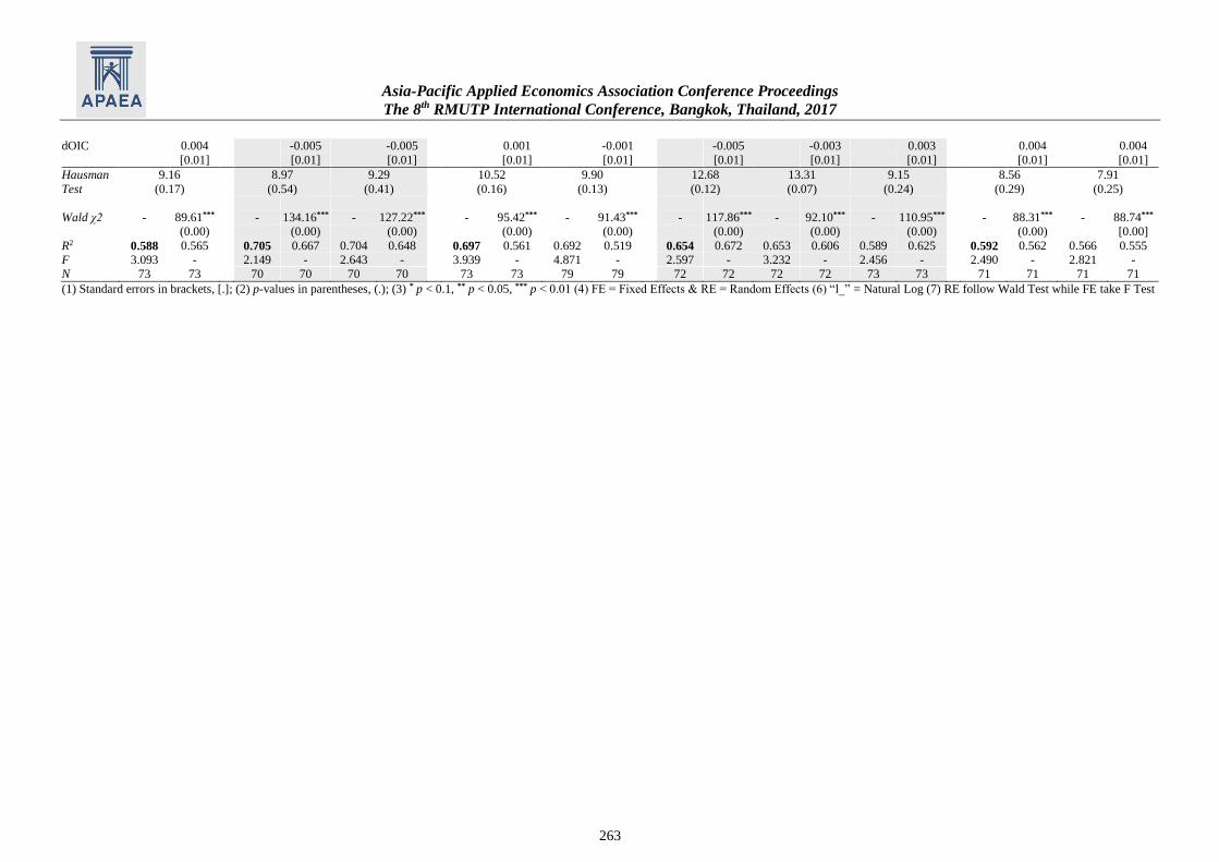
Asia-Pacific Applied Economics Association Conference Proceedings
The 8th RMUTP International Conference, Bangkok, Thailand, 2017
263
dOIC 0.004 -0.005 -0.005 0.001 -0.001 -0.005 -0.003 0.003 0.004 0.004
[0.01] [0.01] [0.01] [0.01] [0.01] [0.01] [0.01] [0.01] [0.01] [0.01]
Hausman 9.16
(0.17)
8.97
(0.54)
9.29
(0.41)
10.52
(0.16)
9.90
(0.13)
12.68
(0.12)
13.31
(0.07)
9.15
(0.24)
8.56
(0.29)
7.91
(0.25) Test
Wald χ2 - 89.61*** - 134.16*** - 127.22*** - 95.42*** - 91.43*** - 117.86*** - 92.10*** - 110.95*** - 88.31*** - 88.74***
(0.00) (0.00) (0.00) (0.00) (0.00) (0.00) (0.00) (0.00) (0.00) [0.00]
R2 0.588 0.565 0.705 0.667 0.704 0.648 0.697 0.561 0.692 0.519 0.654 0.672 0.653 0.606 0.589 0.625 0.592 0.562 0.566 0.555
F 3.093 - 2.149 - 2.643 - 3.939 - 4.871 - 2.597 - 3.232 - 2.456 - 2.490 - 2.821 -
N 73 73 70 70 70 70 73 73 79 79 72 72 72 72 73 73 71 71 71 71
(1) Standard errors in brackets, [.]; (2) p-values in parentheses, (.); (3) * p < 0.1, ** p < 0.05, *** p < 0.01 (4) FE = Fixed Effects & RE = Random Effects (6) “l_” = Natural Log (7) RE follow Wald Test while FE take F Test

Asia-Pacific Applied Economics Association Conference Proceedings
The 8th RMUTP International Conference, Bangkok, Thailand, 2017
264
A2: Pooled OLS (POLS) VS Random Effects (RE)
(1) Standard errors in brackets, [.]; (2) p-values in parentheses, (.); (3) * p < 0.1, ** p < 0.05, *** p < 0.01 (4) POLS = Pooled OLS & RE = Random Effects (6) “l_” = Log (7) RE follow Wald Tes1t while POLS take F Test
W/ ESG ESG Environmental Performance (E) Social Performance (S) Governance Performance (G)
(POLS 1) (RE 1) (POLS 2) (RE 2) (POLS 3) (RE 3) (POLS 4) (RE 4) (POLS 5) (RE 5) (POLS 6) (RE 6) (POLS 7) (RE 7) (POLS 8) (RE 8) (POLS 9) (RE 9) (POLS 10) (RE 10)
Variable ROA ROA ROA ROA ROA ROA ROA ROA ROA ROA ROA ROA ROA ROA ROA ROA ROA ROA ROA ROA
ENV 0.008 0.021** 0.007 0.021** 0.008 0.018** 0.010 0.019**
[0.01] [0.01] [0.01] [0.01] [0.01] [0.01] [0.01] [0.01]
WOEM -0.128*** -0.090** -0.132*** -0.094** -0.124*** -0.088** -0.123*** -0.076
[0.04] [0.04] [0.04] [0.05] [0.04] [0.04] [0.04] [0.05]
ALBGNI 0.014*** 0.014*** 0.013*** 0.012*** 0.014*** 0.013*** 0.014*** 0.012***
[0.00] [0.00] [0.00] [0.00] [0.00] [0.00] [0.00] [0.00]
FeBM 0.020 0.037* 0.011 0.031* -0.000 0.016 -0.006 0.013
[0.02] [0.02] [0.02] [0.02] [0.02] [0.02] [0.02] [0.02]
l_ASST 0.003 0.001 0.006* 0.005 0.003 0.002 0.005 0.003 0.002 0.001 0.006* 0.004 0.004 0.002
[0.00] [0.00] [0.00] [0.00] [0.00] [0.00] [0.00] [0.00] [0.00] [0.00] [0.00] [0.00] [0.00] [0.00]
l_CPB -0.005 -0.000 -0.037*** -0.027*** -0.035*** -0.024** -0.006 -0.002 -0.003 0.000 -0.037*** -0.026*** -0.026*** -0.013 -0.015*** -0.011* -0.005 0.000 -0.003 0.001
[0.00] [0.01] [0.01] [0.01] [0.01] [0.01] [0.01] [0.01] [0.00] [0.00] [0.01] [0.01] [0.01] [0.01] [0.01] [0.01] [0.01] [0.01] [0.00] [0.01]
AEXR -1.348*** -1.294*** -1.339*** -1.323*** -1.354*** -1.336*** -1.375*** -1.363*** -1.330*** -1.337*** -1.320*** -1.250*** -1.405*** -1.321*** -1.263*** -1.215*** -1.350*** -1.295*** -1.352*** -1.298***
[0.16] [0.14] [0.15] [0.14] [0.15] [0.14] [0.16] [0.15] [0.16] [0.14] [0.14] [0.14] [0.15] [0.14] [0.15] [0.14] [0.16] [0.15] [0.16] [0.15]
YGP 0.422*** 0.386*** 0.509*** 0.455*** 0.488*** 0.437*** 0.429*** 0.406*** 0.390*** 0.388*** 0.501*** 0.434*** 0.508*** 0.432*** 0.415*** 0.378*** 0.422*** 0.385*** 0.406*** 0.376***
[0.07] [0.06] [0.07] [0.07] [0.07] [0.07] [0.07] [0.06] [0.07] [0.06] [0.07] [0.07] [0.07] [0.07] [0.06] [0.06] [0.07] [0.07] [0.07] [0.06]
GDPG -0.001 -0.001 -0.002 -0.002* -0.001 -0.002* -0.001 -0.001 -0.001 -0.001 -0.002 -0.001 -0.000 -0.001 -0.002* -0.002 -0.001 -0.001 -0.001 -0.001
[0.00] [0.00] [0.00] [0.00] [0.00] [0.00] [0.00] [0.00] [0.00] [0.00] [0.00] [0.00] [0.00] [0.00] [0.00] [0.00] [0.00] [0.00] [0.00] [0.00]
INF 0.004*** 0.004*** 0.004*** 0.003*** 0.003*** 0.003*** 0.004*** 0.004*** 0.004*** 0.003*** 0.003*** 0.003*** 0.004*** 0.004*** 0.003** 0.003*** 0.004*** 0.004*** 0.004*** 0.004***
[0.00] [0.00] [0.00] [0.00] [0.00] [0.00] [0.00] [0.00] [0.00] [0.00] [0.00] [0.00] [0.00] [0.00] [0.00] [0.00] [0.00] [0.00] [0.00] [0.00]
dOIC -0.002 0.004 -0.013 -0.005 -0.014 -0.005 -0.002 0.001 -0.004 -0.001 -0.014 -0.005 -0.014 -0.003 -0.002 0.003 -0.002 0.004 -0.002 0.004
[0.01] [0.01] [0.01] [0.01] [0.01] [0.01] [0.01] [0.01] [0.01] [0.01] [0.01] [0.01] [0.01] [0.01] [0.01] [0.01] [0.01] [0.01] [0.01] [0.01]
LM Test 24.70***
(0.00)
18.58***
(0.00)
20.31***
(0.00)
26.75***
(0.00)
28.66***
(0.00)
13.29***
(0.00)
14.15***
(0.00)
25.38***
(0.00)
23.78***
(0.00)
7.91
(0.25)
Wald χ2 - 89.61*** - 134.16*** - 127.22*** - 95.42*** - 91.43*** - 117.86*** - 92.10*** - 110.95*** - 88.31*** - 88.74***
(0.00) (0.00) (0.00) (0.00) (0.00) (0.00) (0.00) (0.00) (0.00) (0.00)
R2 0.573 0.565 0.690 0.667 0.674 0.648 0.577 0.561 0.532 0.519 0.683 0.672 0.625 0.606 0.630 0.625 0.575 0.562 0.568 0.555
F 12.47 - 11.75 - 12.18 - 10.91 - 11.53 - 14.84 - 13.11 - 13.65 - 10.47 - 11.82 -
N 73 73 70 70 70 70 73 73 79 79 72 72 72 72 73 73 71 71 71 71

Asia-Pacific Applied Economics Association Conference Proceedings
The 8th RMUTP International Conference, Bangkok, Thailand, 2017
265
A3: List of MFIs that used for the Study # MFI Name Country Region # MFI Name Country Region
1 SEF-ARM Armenia Eastern Europe and Central Asia 32 MCM India South Asia
2 Azercredit Azerbaijan Eastern Europe and Central Asia 33 MBK Ventura Indonesia East Asia and the Pacific
3 SSS Bangladesh South Asia 34 Amartha Microfinance Indonesia East Asia and the Pacific
4 CTS Bangladesh South Asia 35 DEF Jordan Middle East and North Africa
5 Vital Finance Benin Africa 36 NKCF LLC Kazakhstan Eastern Europe and Central Asia
6 Banco FIE Bolivia Latin America and The Caribbean 37 KMF Kazakhstan Eastern Europe and Central Asia
7 CRECER Bolivia Latin America and The Caribbean 38 KosInvest Kosovo Eastern Europe and Central Asia
8 Emprender Bolivia Latin America and The Caribbean 39 WFDF Laos East Asia and the Pacific
9 LIDER Bosnia and Herzegovina Eastern Europe and Central Asia 40 MLF MWI Malawi Africa
10 Partner Bosnia and Herzegovina Eastern Europe and Central Asia 41 XacBank Mongolia Eastern Europe and Central Asia
11 EKI Bosnia and Herzegovina Eastern Europe and Central Asia 42 Ochir-Undraa OMZ Mongolia Eastern Europe and Central Asia
12 PRIZMA Bosnia and Herzegovina Eastern Europe and Central Asia 43 Asasah Pakistan South Asia
13 VisionFund Cambodia Cambodia East Asia and the Pacific 44 Fundación Paraguaya Paraguay Latin America and The Caribbean
14 Chamroeun Cambodia East Asia and the Pacific 45 FINCA - PER Peru Latin America and The Caribbean
15 Fundaci¢n Amanecer Colombia Latin America and The Caribbean 46 MiBanco Peru Latin America and The Caribbean
16 Confiar Colombia Latin America and The Caribbean 47 ADRA Peru Peru Latin America and The Caribbean
17 ADRI Costa Rica Latin America and The Caribbean 48 Manuela Ramos Peru Latin America and The Caribbean
18 Banco ADEMI Dominican Republic Latin America and The Caribbean 49 Microfinanzas PRISMA Peru Latin America and The Caribbean
19 Moris Rasik East Timor East Asia and the Pacific 50 EDPYME Raiz Peru Latin America and The Caribbean
20 VISIONFUND ECUADOR-FODEMI Ecuador Latin America and The Caribbean 51 ASKI Philippines East Asia and the Pacific
21 FACES Ecuador Latin America and The Caribbean 52 NWTF Philippines East Asia and the Pacific
22 CACMU Ecuador Latin America and The Caribbean 53 CEVI Philippines East Asia and the Pacific
23 VF Ethiopia Ethiopia Africa 54 ASA Philippines Philippines East Asia and the Pacific
24 Crystal Georgia Eastern Europe and Central Asia 55 OBS Serbia Eastern Europe and Central Asia
25 Friendship Bridge Guatemala Latin America and The Caribbean 56 FMFB - TJK Tajikistan Eastern Europe and Central Asia
26 ODEF Financiera Honduras Latin America and The Caribbean 57 MDO Arvand Tajikistan Eastern Europe and Central Asia
27 Grameen Koota India South Asia 58 IMON INTERNATIONAL Tajikistan Eastern Europe and Central Asia
28 BISWA India South Asia 59 PRIDE - TZA Tanzania Africa
29 ESAF India South Asia 60 Enda Tunisia Middle East and North Africa
30 Arohan India South Asia 61 CEP Vietnam East Asia and the Pacific
31 Belghoria India South Asia 62 Al Amal Bank Yemen Middle East and North Africa