The 3-Point Method: A Fast, Accurate and Robust Solutionto Vanishing Point Estimation

Vinod Saini, Shripad Gade, Mritunjay Prasad, Saurabh ChatterjeeDepartment of Aerospace Engineering,Indian Institute of Technology, Bombay,

Mumbai, India-400076{ saini.vinod, shripad.gade, mritunjay, saurabhsaurc }@iitb.ac.in

ABSTRACTVanishing points can provide information about the 3D world and hence are of great interest for machine visionapplications. In this paper, we present a single point perspectivity based method for robust and accurate estimationof Vanishing Points (VPs). It utilizes location of 3 collinear points in image space and their distance ratio in theworld frame for VP estimation. We present an algebraic derivation for the proposed 3-Point (3-P) method. Itprovides us a non-iterative, closed-form solution. The 3-P results are compared with ground truth of VP and it isshown to be accurate. Its robustness to point selection and image noise is proved through extensive simulations.Computational time requirement for 3-P method is shown to be much less than least squares based method. The3-P method is extremely useful for accurate VP estimation in structured and well-defined environments.

KeywordsVanishing Points, Point Perspectivity, Length Ratio, Camera Calibration, Cross Ratio

1 INTRODUCTION

A family of parallel lines projected on a plane un-der the pin-hole camera model will ideally intersect ina common point. This point is known as the Vanish-ing Point. VP’s formed by families of coplanar parallellines are collinear and the line is known as the Vanish-ing Line. VPs and Vanishing Lines for an image of acube are shown in Fig. 1.Development of computational techniques and ever-growing requirement of extracting information fromimage have led to a spurt in the field of image analysisin recent years. Vanishing points have myriad applica-tions including camera calibration, robotic navigation,3D reconstruction, pose estimation, augmented realityetc. VP’s have been extensively used for camera cali-bration. [9], [11], [12], [13] and [14] use VPs for cam-era calibration. Image reconstruction problem in [15]and [16] use VP’s for extraction of 3D coordinates ofpoints. [17] uses parallel lines in the environment andcorresponding VP’s for steering a robot. [18] uses van-ishing points and vanishing lines for pose estimation ofUAV’s in indoor flights.

Permission to make digital or hard copies of all or part ofthis work for personal or classroom use is granted withoutfee provided that copies are not made or distributed for profitor commercial advantage and that copies bear this notice andthe full citation on the first page. To copy otherwise, or re-publish, to post on servers or to redistribute to lists, requiresprior specific permission and/or a fee.

Several methods have been proposed to estimate VP’s.[3] uses J linkage based algorithm for vanishing pointestimation in man-made environments. [6] proposes anew framework for line based geometric analysis andVP estimation of Manhattan scenes. [7] uses accuratelylocalised edges that are obtained through edge pixelsand does not require fitting of lines. It uses fewer butmore accurate lines for estimating VPs. [10] relies lineextraction using Hough transform and then on votingin the vanishing point space to estimate VP. All of theabove mentioned methods claim to be accurate for VPestimation in architectural environments e.g. Manhat-tan scenes.

Vanishing points are extremely important in computervision and the accuracy of VP estimation directly influ-ences the performance of the said application. Addi-tionally, since there may be a need to compute vanish-ing points multiple times, a computationally efficientmethod is the need of the day. Camera calibration ef-forts require accurate VP estimates Calibration targetsare well defined structured objects and this informationabout them can be exploited to suit our needs. Fig. 2shows few calibration patterns used in different algo-rithms. [1] proposes two length ratio based methods.First requires evaluation of 1D projective transforma-tion and the direction of lines to compute VP. Seconddetects VP using geometric construction. Here we pro-pose a length-ratio based fast and accurate VP estima-tion method. We use three collinear points and theirdistance ratio in world frame to compute VP location.

Vanishing Lines

Finite Vanishing Point

Figure 1: Vanishing Points and Vanishing Line Figure 2: Patterns used to get VPs

Section 2 discusses camera calibration preliminariesand least squares vanishing point detection method.Section 3 talks about the 3-P method and its formalderivation. Simulation and experimental results are dis-cussed in section 4.

2 PRELIMINARIES2.1 Camera Model

Pin-hole model is based on the principle of collinear-ity, where each point in the world space can be mappedby a straight line to the image plane through the cam-era center. This kind of central projective transform iscalled “Perspective". Fig. 3 shows projection of a lineon image plane. A Pin-hole camera model has beenused here ([1], [2]). Any point P (coordinates given byX) can be mapped to a point p (coordinates given byx) in the image plane . The overall transform can beexpressed as,

x = PX (1)

The overall transformation matrix, P is obtained bymultiplying the extrinsic calibration matrix by intrinsiccalibration matrix. P can be expressed as,

x =K R[I | −C̃]X =KM X = P X (2)

Parameters that are solely dependent on camera arecalled Intrinsic parameters. Principal point, skew, as-pect ratio and focal length together form the intrinsiccamera calibration matrix (K). Extrinsic parameters ofa camera include the rotation and translation of camerawith respect to the world frame. Rotation matrix (R)and translation vectors (C̃) together form the extrinsiccamera calibration matrix (M).

2.2 Least Squares VP estimation

Let us consider a set of n parallel lines in 3D. Ide-ally their mappings in the image plane will intersect ata point (the VP). Due to noise and other errors they willintersect at different points. The maximum number of

intersections that can be found out are nC2. The aim isto estimate a point that has least perpendicular distancefrom the n lines. The methodology can be divided intotwo sub-tasks,

1. Extracting Lines from the image.

2. Finding Least Squares solution.

Extracting Lines Lines can be extracted from the im-age using various image processing techniques. In ourapproach we extract control point locations from theimage (see Figure 8). A least squares fit straight line isdrawn to minimize perpendicular distance of m pointsfrom the line. If (xi,yi) are the locations of the m pointsthat lie on a straight line, the slope (slope) and intercept(c) of the line are given by,[

cslope

]=

[m ∑

mi=1 xi

∑mi=1 xi ∑

mi=1 x2

i

]−1 [∑

mi=1 yi

∑mi=1 xiyi

](3)

Least Squares solution Once the line information isextracted from the image, the only hurdle in estimatingthe vanishing point using least-squares is finding the in-tersection of lines. For any two points vi and v j, the linepassing through them can be expressed as,

Li j = vi× v j

If m lines given by Li (i=1,2,...,m) intersect in a point V ,then the coordinates of V are given by,LT

1..

LTm

VxVyVz

= 0 (4)

3 THE 3-POINT METHOD

Parallel lines appear to intersect at a point in perspec-tive view. In an image this perspectivity is introduceddue the camera parameters and its orientation. Sev-eral methods have been proposed in literature to mea-sure perspectivity. In [1] this perspectivity is measured

Figure 3: Pin-hole camera model Figure 4: Length Ratio for 3-P method

through the evaluation of 1D projective transformation.The main idea behind our method is that we can geta sense of this camera perspectivity through the threecollinear points from the image and their length ratio inthe world frame.

Let us consider a family of parallel lines representedby F . These lines are projected onto an image planethrough a pin-hole camera model. Let this set be calledas F. Now, if we select two points lying on any linef ( f ∈ F) ; we can write the equation of that line fin image space. Equation of line f and the length ratio(given by three collinear points) in the world frame willprovide information about perspectivity along f. Thiswill enable us to map any point on line f (f∈F ) onto itsimage f (f ∈ F). Any point on line f at infinite distancewhen mapped under pin-hole camera model will maponto VP.

The advantage of this method over the length ratiomethod is that it does not require us to compute ho-mography (projective transform) and perform intensivecomputations. It provides us with a closed-form so-lution and is computationally efficient. Line detectionand clustering is not required in this method. This re-duces computational load significantly and altogethereliminates line detection and clustering errors. Also thismethod can be made to utilize information from a smallregion in the image, thereby reducing errors due to de-focusing of certain parts of image.

3.1 Derivation

Let us consider three collinear points A(x1,y1,z1),B(x2,y2,z2) and C(x3,y3,z3). Let, the line that passesthrough them be called L1 as shown in Fig. 3.Distance Ratio: The distance ratio for three collinearpoints is given by (see Fig. 4),

Γ =dAC

dAB=

√(x1− x3)2 +(y1− y3)2 +(z1− z3)2√(x1− x2)2 +(y1− y2)2 +(z1− z2)2

(5)

Camera Model: We use a pin-hole camera model withprojection matrix P. Let the images of A, B and C

be called A’(u1,v1,1), B’(u2,v2,1) and C’(u3,v3,1) re-spectively.

A′ = PA, B′ = PB, and C′ = PC (6)

Line L1: Equation of line L1 (see Fig. 3) can be writtenin the two point form (using points A and B) as follows,

x− x1

x2− x1=

y− y1

y2− y1=

z− z1

z2− z1= λ (7)

orx = x1 +λ (x2− x1)y = y1 +λ (y2− y1)z = z1 +λ (z2− z1)

(8)

Now, if we substitute coordinates of point C in Eq. (8)and use the expression in Eq. (5) we can easily con-clude that Γ and λ are equal.Coordinates of C′, for a known distance ratio, can beexpressed as,

w3u3w3v3

w3

= P

x1 + λ (x2 − x1)y1 + λ (y2 − y1)z1 + λ (z2 − z1)

1

= P

x1y1z11

+ λP

x2 − x1y2 − y1z2 − z1

0

=

w1u1w1v1w1

+ λ

w2u2 − w1u1w2v2 − w1v1

w2 − w1

(9)

Simplifying the above equation we get C’ as,

(u3,v3) =(

u1+λ (αu2−u1)1+λ (α−1) , v1+λ (αv2−v1)

1+λ (α−1)

)(10)

where, α is defined as w2w1

.

For any point D(x,y,z) lying on line L1, and the imageD’(u,v,1) are related by D′ = PD. The coordinates ofD’ are obtained by Eq. 10, and expressed as,

(u,v) =(

u1+λ ′(αu2−u1)1+λ ′(α−1) , v1+λ ′(αv2−v1)

1+λ ′(α−1)

)(11)

X1'

X2'

X3'

X4'

X1 X2 X3 X4

O

Image Plane

Figure 5: Cross Ratio

Optimal L

ine

Optimized Points

Noisy Points

P1

P1’

P2

P2’

Pn’

Pn

Figure 6: Noisy image points and its projection on bestfit line

In homogenous coordinates, (wu,wv,w) and (u,v,1)represent the same point. The factor w is merely ascaling quantity. The parameter α is defined as theratio of scaling factors for two different points. Itthereby provides wisdom about perspectivity. α can beevaluated from Eq. 10.

α =w2

w1=

(u3−u1)(λ −1)(u3−u2)λ

(12)

The vanishing point is the image of a point lying at in-finity on line L1. This point (let us say is D) in theworld frame will have a distance ratio, (λ ′ = dA,D

dA,B)) of

∞. To get the VP, we substitute this value of λ ′ in Eq.11. Through algebraic manipulation, we get,

(V Px,V Py) =(

αu2−u1α−1 , αv2−v1

α−1

)(13)

An interesting phenomenon can be observed if we con-sider an image with zero perspective. For such an imageα is equal to 1 since the scaling factors will be same forboth the points. VP for such an image will be located at∞ (Eq. 13). This is to be expected, since VPs arise onlydue to perspective in the image.

3.2 Proof by InvarianceProperty: The cross ratio (χ) is invariant under projec-tive transformation. χ is expressed as,

χ =d13d24

d12d34(14)

where di, j represents distance between points i, j asshown in Fig. 5.

In our current formulation let us assume that a fourthpoint V is lying on line L1 at an infinite distance alongwith A, B and C. V’ projected on the image plane fromV, will represent the vanishing point. Using Eq. 5, crossratio in world frame is given by,

χ = limV→∞

dABdCV

dACdBV=

1λ

limV→∞

(1+dCB

dBV) =

1λ

(15)

In the image frame, let the coordinates of V’ be givenby Eq. 13, We write the cross ratio as,

χ′ =

√(u1 − u2)2 + (v1 − v2)2√(u1 − u3)2 + (v1 − v3)2

×

√( u3−u3α−u1+u2α

1−α)2 + ( v3−v3α−v1+v2α

1−α)2√

( u2−u11−α

)2 + ( v2−v11−α

)2

(16)

Substituting the value of α from Eq. 12 and simplifyingalgebraically, we get χ = χ ′. This shows that the crossratio of four points is invariant under projection and ourVP estimates are accurate.

3.3 Tackling Noise

In the presence of noise, the performance of imageprocessing techniques may get degraded. If the locationof those three collinear points is not known precisely,errors will creep in to the VP estimates. To reduce thissensitivity we incorporate a least squares based opti-mization method. The idea behind this method is todraw a least square fit line from the selected three pointsto find the direction. Then orthogonally project thesepoints on this line. These new points are used in placeof earlier noisy data see Fig. 6.

4 RESULTS

Experiments were performed to validate the 3-Point(3-PVP) method. Robustness of the method and itscomputational efficiency are investigated through sim-ulations. All simulations are performed in MATLAB R©environment. Simulations were performed on a PC withi5 processor (3.2 GHz, 64 bit) and 4 Gb RAM.

[3] and [6] focus on vp estimation in urban/man-madeenvironment where determining distance ratio willbe difficult and will have to be separately estimated.Hence, we compare our results with LSVP methoddescribed in Section 2.

0 50 100 150 200 250 300 350 400 4500

50

100

150

200

250

300

350

400

X Pixel

Y P

ixe

lSimulated Image with 10 × 10 Control Points

Figure 7: Simulated Pattern of 10×10 control points Figure 8: Metal fixture with 10×10 control points

4.1 Simulation

We here simulate perspectivity transform and gen-erate synthetic images. A target pattern with 10× 10evenly distributed points is simulated as shown in Fig.7. Two sets of parallel lines can be drawn in X andY direction. This pattern is projected on the syntheticimage-plane using a simulated camera. Properties aretabulated in Table 1.Absolute ground truth can be found out for simulatedimages and hence it can be a great tool to validate es-timation method. Since, we are simulating perspective,the camera matrix P is known to us and homogenouscoordinates (of infinity point along the line) are knownto be [1,0,0,0].Synthetic images provide us with an unique opportunityto add Gaussian noise and analyse robustness. Gaussiannoise N (0,0.1px) is added to each projected point onthe pattern. This new noisy image is given as input tothe VP estimation algorithm. Two vanishing points areestimated in each image, represented by VP1 and VP2.We perform 100 Monte-Carlo runs for both methods.

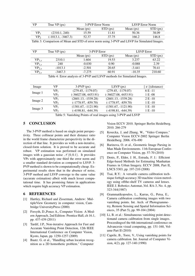
Accuracy and RobustnessWe compare our results with least square approach. 3-PVP provides accurate VP estimates. This is seen fromthe fact that 3-PVP estimates are closer to the groundtruth. The mean error and standard deviation of errorare also lower for 3-PVP as compared to LSVP. Themean errors are negligibly small as compared to VP es-timate for both methods. Standard deviation of error isapproximately one third the value of LSVP. Results aretabulated in Table 4.Noise with std of 0.1 px was used to study robustness.3-PVP method is shown to be robust to image noise.Euclidean norm of error is much higher for LSVP ascompared to 3-PVP. Error norm for LSVP is approxi-mately three times that of 3-PVP. Error values are tabu-lated in Table 3

Parameter ValueFocal Length 50 mm

Principal Point (360,240) pxSkew Factor 0Scale Factor 1

Orientation Vector [00 400 300]Translation Vector [800,−1200,300] mmImage Resolution 720 × 480

Table 1: Simulated camera parameters

Fig. 9 and Fig. 10 shows the ground truth locationof VP and the spread of estimated VPs using bothmethods. The VPs estimated by LSVP have moredeviation from the true value. Fig. 11 represents theerror in x and y direction along with error norm for theMonte-Caro runs. 3-PVP method shows lesser error ascompared to LSVP.

Computational CostMonte-Carlo runs also can indicate the computationalcost of the algorithm. The time taken by both meth-ods are tabulated in Table 2 for 100, 1000 and 10000runs. We can observe that the speed of 3-PVP is ap-proximately ten times faster. LSVP method involvesfirstly forming least square lines and secondly findingtheir intersection. 3PVP on the contrary employs an al-gebraic relation and is hence fast. These simulationsvalidate our method’s accuracy, robustness and speed.

Runs 3-PVP (s) LSVP (s)100 0.23 1.27

1000 1.51 13.0910000 14.94 132.65

Table 2: Simulation Time

4.2 Experimental ResultsThe target used for validating the 3-P VP method is

shown in Fig. 8. The coordinates of the center of cir-cles are known with high degree of accuracy. These

−1500 −1000 −500 0 500 1000 1500 2000 2500−4000

−3500

−3000

−2500

−2000

−1500

−1000

−500

0

500

X (Px)

Y (

Px)

100 Monte Carlo Runs − (3−PVP)

Estimated VP1

Estimated VP2

True VP1

True VP2

Figure 9: VP estimate spread for 3-PVP

−1500 −1000 −500 0 500 1000 1500 2000 2500−4500

−4000

−3500

−3000

−2500

−2000

−1500

−1000

−500

0

500

X (Px)

Y (

Px)

100 Monte Carlo Runs − (LSVP)

Estimated VP1

Estimated VP2

True VP1

True VP2

Figure 10: VP estimate spread for LSVP

10 20 30 40 50 60 70 80 90 100

−100

0

100

200

VP1 Error in X Direction

Err

or(

Px)

Number of Runs10 20 30 40 50 60 70 80 90 100

−5

0

5

VP1 Error in Y Direction

Err

or(

Px)

Number of Runs

10 20 30 40 50 60 70 80 90 100

−100

0

100

VP2 Error in X Direction

Err

or(

Px)

Number of Runs10 20 30 40 50 60 70 80 90 100

−400

−200

0

200

400

VP2 Error in Y Direction

Err

or(

Px)

Number of Runs

10 20 30 40 50 60 70 80 90 100

50

100

150

200

Error Norm of VP1

Err

or

(Px)

Number of Runs10 20 30 40 50 60 70 80 90 100

200

400

600

Error Norm of VP2

Err

or

(Px)

Number of Runs

LSVP

3PVP

Figure 11: Error in VP Estimates (RMS, X & Y Direction) for 3-PVP v/s LSVP

points are planer in nature and form two sets of paral-lel lines. The image is captured using a Cannon EOS1100 D camera with fixed effective focal length of 50mm. Median filter has been used to remove noise fromthe image. A well-focused image of the target is pro-cessed in MATLAB to obtain centroids of the circularcontrol points. Two vanishing points are obtained fromeach image. The vanishing points obtained by the 3-pstrategy are compared with results from LSVP method.

3-PVP and LSVP are used on three images and theirVPs are estimated. The results show that both the meth-ods work effectively with the current image. The dis-tance between results from both methods is shown tobe of the order of 10−08 or lower. This also shows thatin the absense of noise both methods will converge tothe same estimate. VP estimates for those three imagesare tabulated in Table 5. Advantages of our method are,

• Tackling of radial distortion: Our algorithm givesus the freedom to select the three points, which canbe selected such that they lie in the middle of theimage. Radial distortion effects are negligible nearthe center.

• Handling defocused images: Partial defocusing inimages can lead to large erros in feature extraction.We can select required three points in such a waythat you avoid defocused parts of the image.

• Independent of Parallel Lines: Errors also creep inwhen the given set of lines is not perfectly paral-lel. We do not need parallel lines and hence are notprone to errors.

• Speed and Robustness

VP True VP (px) 3-PVP Error Norm LSVP Error NormMean (px) STD (px) Mean (px) STD (px)

VP1 (2310.1, 240) 15.59 11.81 50.36 38.09VP2 (-1013.1, -3467.3) 52.37 37.75 166.2 146.8

Table 3: Comparison of Mean and STD of error norm using 3-PVP and LSVP for Simulated Images.

VP True VP (px) 3-PVP Error LSVP ErrorMean (px) STD (px) Mean (px) STD (px)

VP1,x 2310.1 1.604 19.53 3.237 63.22VP1,y 240 -0.030 0.90 -0.088 2.39VP2,x -1013.1 -2.501 20.65 -3.441 70.41VP2,y -3467.3 -7.275 60.91 -10.35 210.60

Table 4: Error analysis of 3-PVP and LSVP methods for Simulated Images.

Image VP 3-PVP (px) LSVP (px) ‖ ε ‖(distance)

Image 1 VP1 (279.45, -1179.07) (279.45, -1179.07) 6 E -11VP2 (-36027.08, 4453.91) (-36027.08, 4453.91) 1 E -08

Image 2 VP1 (2601.13, -1539.28) (2601.13, -1539.28) 2 E -10VP2 (-1778.97, -859.70) (-1778.97, -859.70) 1 E -10

Image 3 VP1 (1301.67, -1121.90) (1301.67, -1121.90) 1 E -10VP2 (-4198.81, -644.39) (-4198.81, -644.39) 1 E -10

Table 5: Vanishing Points of real images using 3-PVP and LSVP

5 CONCLUSION

The 3-PVP method is based on single point perspec-tivity. Three collinear points and their distance ratioin the world frame characterize perspectivity in the di-rection of that line. It provides us with a non-iterative,closed-form solution. It is proved to be accurate androbust. VP estimation was performed on simulatedimages with a gaussian noise N (0,0.1). It providesVPs with approximately one third the error norm anda smaller standard deviation as compared to LSVP. 3-PVP method is shown to be computationally cheap. Ex-perimental results show that in the absence of noise,3-PVP method and LSVP converge to the same value(accurate estimation) albeit with much lesser compu-tational time. It has promising future in applicationswhich require high accuracy VP estimation.

6 REFERENCES[1] Hartley, Richard and Zisserman, Andrew: Mul-

tipleView Geometry in computer vision, Cam-bridge UniversityPress (2000)

[2] Forsyth, D.,Ponce A., Computer Vision: A Mod-ern Approach, 2nd Edition: Prentice Hall, ch 16.1,pp. 437-439 (2011)

[3] Tardif, J.P., Non-iterative Approach for Fast andAccurate Vanishing Point Detection, 12th IEEEInternational Conference on Computer Vision,Kyoto, Japan, pp. 1250-1257 (2009)

[4] Baatz. G. et al., "Handling urban location recog-nition as a 2D homothetic problem." Computer

Vision ECCV 2010. Springer Berlin Heidelberg.2010. 266-279

[5] Kosecka, J, and Zhang, W., "Video Compass."Computer Vision ECCV-2002 Springer BerlinHeidelberg. 2006. 476-490

[6] Barinova, O. et al., Geometric Image Parsing inMan Made Environments. 11th European Confer-ence on Computer Vision, pp. 57-70 (2010)

[7] Denis, P., Elder, J. H., Estrada, F. J.: EfficientEdge-based Methods for Estimating ManhattanFrames in Urban Imagery. ECCV 2008, Part II,LNCS 5303, pp. 197-210 (2008)

[8] Tsai, R.Y.: A versatile camera calibration tech-nique forhigh accuracy 3D machine vision metrol-ogy using offthe-shelf TV cameras and lenses.IEEE J. Robotics Automat.,Vol. RA-3, No. 4, pp.323-344(1987)

[9] Grammatikopoulos, L., Karras, G., Petsa, E.,Camera calibration combining images with twovanishing points. Int. Arch. of Photogramme-try, Remote Sensing and Spatial Information Sci-ences, 35 (Part 5), pp. 99-104 (2004)

[10] Li, B. et al.: Simultaneous vanishing point detec-tionand camera calibration from single images.Proceedingsof the 6th international conference onAdvancesin visual computing, pp. 151-160, Vol-ume Part II (2010)

[11] Caprile, B., Torre, V., Using vanishing points forcamera calibration. Int. Journal of Computer Vi-sion, 4(2), pp. 127-140 (1990)

[12] Lee, D. H., Jang K. H., and Jung, S. K.: Intrin-sic Camera Calibration Based On Radical CenterEstimation. The 2004 International Conferenceon Imaging Science, Systems, and Technology,USA, pp. 7-13, (2004)

[13] He. B.W., Li Y.F., Camera calibration from van-ishing points in a vision system, Optics and LaserTechnology, Volume 40, pp. 555-561(2008)

[14] Orghidan, R. et al.: Camera calibration usingtwo or three vanishingpoints, Proceedings of theFederated Conference onComputer Science andInformation Systems, pp. 123-130 (2012)

[15] Fong, C.K.: 3D object reconstruction from sin-gle distortedline drawing image using vanishingpoints. Proceedings of ISPACS 2005 pp. 53-56

(2005)[16] Parodi, P. and Piccioli, G.: 3D shape reconstruc-

tionby using vanishing points. IEEE Transactionson Pattern Analysis and Machine Intelligence,vol. 18,no. 2, pp. 211-217 (1996)

[17] Schuster, R., Ansari, N. and Bani-Hashemi,A.:Steering a Robot with Vanishing Points. IEEE-Transactions on Robotics and Automation,Vol. 9,NO. 4, pp. 491-498 (1993)

[18] Wang, Y.: An efficient algorithm for UAV in-doorpose estimation using vanishing geometry.12th IAPRConference on Machine Vision Appli-cations, Japan, pp. 361-364 (2011)