textile science & engineering - omics international device has a different gamut and its own...

Volume 1 • Issue 1 • 1000102J Textile Sci EnggISSN: 2165-8064 JTESE, an open access journal

Open Access

Shams-Nateri, J Textile Sci Engg 2011, 1:1 DOI: 10.4172/2165-8064.1000102

Open Access

Research Article

Measuring Reflectance Spectra of Textile Fabrics by ScannerA. Shams-Nateri*

Textile Engineering Department, University of Guilan, Rasht, Iran

*Corresponding author: A. Shams-Nateri, Textile Engineering Department, University of Guilan, Rasht, Iran, E-mail: [email protected]

Received October 24, 2011; Accepted November 19, 2011; Published November 21, 2011

Citation: Shams-Nateri A (2011) Measuring Reflectance Spectra of Textile Fabrics by Scanner. J Textile Sci Engg 1:102. doi:10.4172/2165-8064.1000102

Copyright: © 2011 Shams-Nateri A, et al. This is an open-access article distributed under the terms of the Creative Commons Attribution License, which permits unrestricted use, distribution, and reproduction in any medium, provided the original author and source are credited.

Keywords: Scanner; Reflectance estimation; Principal componentanalysis; Polynomial regression; Neural network; Neuro-fuzzy

IntroductionA calibration procedure is unavoidable for high quality color

reproduction by low-cost color devices such as digital color cameras, scanner etc. Each device has a different gamut and its own color space defined by the relationship between the input colors and the corresponding RGB codes used to represent them. A simple method of converting scanner or digital camera RGB responses to estimates of object tristimulus coordinates is to apply a linear transformation to the RGB values. The transformation parameters are selected subject to minimization of some significant error measure. The basic idea of color target-based characterization is to use a reference target that contains a certain number of color samples. Typical methods like least squares polynomial modeling tristimulus, neural networks and three-dimensional lookup tables with interpolation and extrapolation can be used to derive a transformation between RGB values and XYZ values [1-8].

Estimation spectral information from digital color image has become a field of much interest and practical importance during the last few years. The color reproduction based on trichromatic data is often insufficient to obtain the device in dependent color, e.g. XYZ. In addition, an accurate illumination correction is impossible from tri chromatic data, which is required when the color image is reproduced under different illuminations from the one used in the recording. Conversely, the spectral reflectance of an object is its intrinsic characteristic, which can be obtained by recording a spectral reflectance image. The device independent color under the any illumination light can be cal culated from spectral reflectance. Various kinds of multi-band cameras have been developed for the pur pose of spectral reflectance image achievement. A considerable number of studies have been also conducted on the spectrum estimation method from multi-band image data. A practical problem in the estimation of spec tral reflectance images is that spectrum estimation depends on the spectral prop erties of the camera and the light illuminating the object. In order to obtain their properties, a spectral measurement device, such as spectropho tometer, is generally used [3,4,7-11].

The spectral characterization consists in approximating the different spectral characteristics of the sensor. A multispectral image is an image where each pixel contains information about the spectral reflectance of the imaged scene. Multispectral images carry information about a number of spectral bands: from three components per pixel for RGB color images to several hundreds of bands for hyperspectral images.

Multispectral imaging is relevant to several domains of application, such as remote sensing, astronomy, medical imaging, and analysis of museological objects, cosmetics, medicine, high-accuracy color printing, or computer graphics. Multispectral scanners are mostly based on a point-scan scheme and are thus too slow and expensive [12,13].

Principal component analysis is a basis of new statistical method for data analysis. This has been used in data analysis and compression. Principal component analysis is a basis of latest data analysis, which has been called one of the most important results from applied linear algebra. PCA is used abundantly in all forms of analysis such as neuroscience and image processing. It is a simple, non-parametric method of extracting relevant information from confusing data sets. Principal components analysis generates a new set of variables, called principal components. Each principal component is a linear combination of the original variables and all the principal components are orthogonal to each other. There are numerous ways to construct an orthogonal basis for a set of spectral data. The first principal component accounts for as much of the variability in the data as possible, and each subsequent component accounts for as much of the remaining variability as possible. By grading the eigenvectors for descending eigenvalues, so that largest is first, one can create an ordered orthogonal method with the first eigenvector having the direction of largest variance of the data. In this way, we can find directions in which the data set has the most significant amounts of energy and variation [13-19].

In color science, principal component analysis has been used mainly for data compression and defines the principal directions that a set of data orient. A number of researchers have since investigated to estimation spectral information from tristimulus and application of principal components analysis in the recovering spectral information. The colorimetric data can be easily calculated from spectral data, but the computation of spectral data from colorimetric values is not

AbstractThis study presents a practical approach for estimation reflectance spectra by means of scanner. New methods

were based on polynomial regression, neural network, neuro-fuzzy and principal component analysis techniques. Obtained results indicate that the recovery error decreases with increase number of principal component and number of terms in a polynomial. Also, application of principal component increase accuracy of reflectance measurement. The best estimation is obtained by principal component analysis and artificial neural network (PCA- ANNET) with 0.0297 RMS and 6.14 ∆E*ab error.

Journal of Textile Science & EngineeringJo

urna

l of T

extile

S cience &Engineering

ISSN: 2165-8064


of 13


similarly possible. The three-dimensional color data such as tristimulus value is insufficient for accurate estimation of reflectance spectra of the material. Several papers have been published attempting to solve this problem in extract the reflectance data from the corresponding tristimulus values. Several mathematical techniques such as simulated annealing method, application of ideal subtractive or additive Gaussian primaries, simplex method have been used for the reconstruction of reflectance spectra of samples from their corresponding tristimulus. Among them, the principal component analysis has been widely used for the reconstruction reflectance spectra. The recovery performance of the method mostly depends on the number of principal components, which have been chosen for estimation reflectance spectra [17-20].

Neural network

Recently, many researches have utilized a parallel processing structure that has a large number of simple processing with many interconnections between them. The use of these processors is much simpler and faster than one central processing unit. Because of recent advantages in technology, the neural network has emerged as a new technology and has found wide application in many areas. In this work, the multi-layer perceptron was used to process data by using the modified back-propagation algorithm. This algorithm attempt to minimize an error function by modification of network connection weights and bias. In each iteration, an input vector is presented to the network and propagated forward to determine the output signal. The output vector is then compared with the target vector resulting an error signal, which is backed propagated through the network in order to adjust the weights and bias. This learning process is repeated until the network respond for each input vector with an output vector that is sufficiently close to the desired one [21-24].

Neuro-fuzzy

The fuzzy inference system (FIS) is a computing system based on the concepts of fuzzy set theory, fuzzy IF/THEN rule and fuzzy reasoning to make relationship between an input space into an output space. The basis for fuzzy logic is the basis for human communication. Fuzzy reasoning contains very simple mathematical concepts. The fuzzy system can match any set of input-output data. This process is made particularly easy by adaptive techniques like adaptive neuro-fuzzy inference systems. ANFIS is about taking a fuzzy inference system and training it with a backpropagation algorithm, well known in the artificial neural network (ANN) theory, based on some collection of input/output data. The basic structure of fuzzy inference system consists of three conceptual components: A rule base, database or dictionary which defines the membership functions used in the fuzzy rules, and reasoning mechanism which performs the inference procedure upon the rule and a given condition to derive a reasonable output or conclusion [25-27].

The present study describes a new technique based on principal component analysis, polynomial regression, neural network and neuro-fuzzy techniques that attempts to reconstruction reflectance spectra from the scanner RGB values.

Materials and MethodsThe Benq 5550T color scanner was used for scanning and imaging

the colored fabrics. The fabrics were scanned under the condition of 600 pixels/inch and 24 bit /pixel. The reflectance spectra of dyed fabrics were measured by using Texflash spectrophotometer of Datacolor Corporation. The colored fabrics were consisting of polyester fabrics

dyed with disperse dyestuff in varieties of colors. The chromaticity of fabrics is shown in Figure 1 under condition of 10 degree standard observer and D65 illuminant. A set of 141 patches of fabrics were used as training data and 41 patches were kept for testing. The lightness of training and testing samples are shown in Figures 2 and 3, respectively. All computations were performed by using MATLAB software.

sRGB method

In this method, the relationship between the reflectance spectra and scanner RGB values was obtained by using sRGB equation. The experimental procedure is outlined below:

• Scan fabrics by scanner and obtain the scanner RGB responses from colored fabrics images.

• Then RGB value of scanner was converted to CIEXYZ by follow:

255

255

255

= =

=

RR

GG

BB

(1)

2.4

0.0404512.92

0.055 0.040451.055

≤=

+ >

R Rr

R R 2)

2.4

0.0404512.92

0.055 0.040451.055

≤=

+ >

G Gg

G G

(3)

2.4

0.0404512.92

0.055 0.040451.055

≤=

+ >

B Bb

B B

(4)

100

100

100

= × = ×

= ×

R r

G g

B b (5)

0.4124 0.3576 0.1805

0.2126 0.7152 0.0722

0.0193 0.1192 0.9505

= × + × + × = × + × + ×

= × + × + ×

X R G B

X R G B

Z R G B

(6)

•Measuring the reflectance spectra of training samples by spectrophotometer.

•Calculating principal components of reflectance spectra.

•Calculating the tristimulus of principal components (XYZPC):

,100

λ λ λλ

= × ×∑i iX E PC xK

(7)


of 13


XYZ are tristimulus values of testing samples which is evaluated in previous stage. XYZPC is tristimulus of principal components with highest eigenvalue.

• Application: calculating reflectance spectra by using principal component weighting (transformation matrix) in Equation 11.

1 1 2 2...........................= × + × + ×n nR m PC m PC m PC (11)

XYZ-polynomial regression method

In this method, the relationship between the reflectance spectra and scanner RGB values was obtained by means of polynomial regression technique. The experimental procedure is outlined below:


• Measure the reflectance spectra and CIEXYZ values of colored fabrics by spectrophotometer.

• Derive a transfer matrix that matches scanner RGB to CIEXYZ values of color fabrics by multiple polynomial regression by Equation 12. The polynomial functions are shown in Table 1.

( , , , ) = ×

XY M h m R G BZ

(12)

• Measuring the reflectance spectra and the tristimulus values (XYZ) of training samples by spectrophotometer.

• Calculating principal components of reflectance spectra.

• Calculating the tristimulus of principal components (XYZPC) by equations 7, 8 and 9.

• Calculating the transformation matrix (principal component weighting) by Equation 10.


PCA-polynomial regression method

The relationship between the reflectance spectra and scanner RGB values was achieved by means of polynomial regression and principal component analysis techniques. The procedure of calibration is outlined below:

• Scan samples by scanner and obtain the scanner RGB responses from their image.

• Measure the reflectance spectra of samples by spectrophotometer.

• Calculating principal components of reflectance spectra of training dataset.

• Calculating principal component weighting.

• Obtain the conversion polynomial function (A) between scanner polynomial function (h(n, R, G, B)) and principal component weighting (Mn):

( ( , , , ))= ×n nA M pinv h n R G B (13)

where Mn is weighting of n principal components and An is a n×n

Figure 1: Chromaticity distribution of training and testing samples.

Training samples Testing samples

-110

-60

-10

40

90

-100 -50 0 50 100

b*

a*-110

-60

-10

40

90

-100 -50 0 50 100

b*

a*

0

10

20

30

40

50

60

70

80

90

100

1 9 17 25 33 41 49 57 65 73 81 89 97 105 113 121 129 137

L*

Sample

Figure 2: The lightness of training samples.

,100

λ λ λλ

= × ×∑i iY E PC yK

(8)

,100

λ λ λλ

= × ×∑i iZ E PC zK

(9)

where λ λλ

= ×∑K E y , i =1, …, n and n is number of principal components

• Calculating the transformation matrix by Equation 4:

1( )−= × pcM XYZ XYZ (10)

where M is transformation matrix (principal component weighting),

0

10

20

30

40

50

60

70

80

90

100

1 3 5 7 9 11 13 15 17 19 21 23 25 27 29 31 33 35 37 39 41

L*

Sample

Figure 3: The lightness of testing samples.


of 13


matrix of coefficients, h(n, R, G, B) is a vector of scanner output signals polynomial function, where n is the number of terms in a polynomial and number of principal components at each model. Various polynomial transform functions were applied as detailed in Table 2.

• Application: convert scanner RGB into transformation matrix

by obtained function in Equation 14.

2,2 2,2 2,2

,1 ,2 ,

1,1 1,2 1,1

. . . .

. . . .

. . . .. ( , , , )

. . . .

. . . .

. . . .

. . . .

= ×

n

n n n n n

na a ama a am

h n R G B

m a a a

(14)

Calculate reflectance spectra by using principal component weighting and average of training samples reflectance spectra in Equation 15.

1 1 2 2 .............= + × + × + ×m n nR R m PC m PC m PC (15)

ANNET method

In this method, the relationship between the reflectance spectra and scanner RGB values was obtained by means of artificial neural network. The experimental procedure is outlined below:


• Measure the reflectance spectra values of training samples by spectrophotometer.


• The used multilayer perceptrons neural networks contain three inputs as scanner RGB responses, and three outputs as CIEXYZ values. Figure 4 shows the structure of neural network with three inputs, three outputs and one hidden layer, which contain 4 nodes. The topologies details of neural networks are shown in Table 3.

• The neural network was trained with backpropagation algorithm, which was continued over 500 epochs. The trained neural networks were used to evaluate the CIEXYZ values of testing samples from their RGB values.

• Measuring the reflectance spectra of training samples by spectrophotometer


• Calculating the tristimulus for principal components by Equations 7, 8 and 9.

• Calculating the transformation matrix (principal component weighting) by Equation 10:


PCA-ANNET method

In this section, neural network and principal component analysis were used for construction relationship between the reflectance spectra and scanner RGB values. The experimental procedure is outlined below:

No. Number ofterms Polynomial terms ( ),,,( BGRmh )

1 3 R G B

2 4 R G B 1

3 7 R G B R2 G2 B2 1

4 8 R G B R×G R×B G×B R2 G2 B2 1

5 14 R G B R×G×B R×G R×B G×B R2 G2 B2 R3 G3 B3 1

Table 1: Polynomial regression function.

No.Number

ofPCA

number of terms Polynomial terms ( ( , , , )h m R G B )

1 3 3 R G B

2 3 4 R G B 1

3 3 7 R G B R2 G2 B2 1

4 3 8 R G B R×G R×B G×B R2 G2 B2 1

5 3 14 R G B R×G×B R×G R×B G×B R2 G2 B2 R3 G3 B3 1

6 4 7 R G B R2 G2 B2 1

7 4 8 R G B R×G R×B G×B R2 G2 B2 1


9 5 7 R G B R2 G2 B2 1

10 5 8 R G B R×G R×B G×B R2 G2 B2 1


Table 2: Polynomial regression function.

Figure 4: Structure of neural network with three output.

No. Number ofterms mean max min SD

1 3 0.0899 0.1675 0.0413 0.0343

2 4 0.0806 0.1647 0.0236 0.0387

3 7 0.0865 0.2740 0.0199 0.0601

4 8 0.0852 0.2555 0.0133 0.0599

5 14 0.0820 0.2001 0.0083 0.0549

Table 3: The spectrophotometric accuracy of polynomial regression (RMS).


of 13


• Scan samples by scanner and obtain the scanner RGB responses from their image.

• Measure the reflectance spectra of samples by spectrophotometer.


• Calculating principal component weighting.

• Neural networks with multi-layer perceptron configuration applied to conversion scanner RGB values to principal component weighting. The neural network has 3 inputs as scanner RGB values and three to five outputs as coefficients first principal components (Figure 5). Several topologies were tested to make relation between principal component weighting and scanner RGB values. The neural network was trained with backpropagation algorithm. The error goal was 0.0001 and neural network training was continued over 1000 epochs by back propagation algorithm.

• Application: convert scanner RGB into principal component weighting by trained neural network and calculate reflectance spectra by means of principal component weighting (Equation 15).

Neuro-Fuzzy method

In this method, the relationship between the reflectance spectra and scanner RGB values was obtained by means of neuro-fuzzy. The experimental procedure is outlined below:


• Measure the reflectance spectra and CIEXYZ values of training samples by spectrophotometer.

• Three ANFIS systems have been used. Each system has three input nods referred to the scanner RGB values and one output referred to one of the tristimulus values (Figure 6). Several membership functions such as gbellmf (Generalized bell-shaped built-in membership function), gauss2mf (Gaussian combination membership function), gaussmf (Gaussian curve built-in membership function) and dsigmf (Built-in membership function composed of the difference between two sigmoidal membership functions) were used for input nodes. Different numbers of membership functions have been also used for each input node. The neuro-fuzzy system has been trained by a hybrid method consisting of back propagation for the parameters associated with the input membership

functions, and the least squares estimation for the parameters associated with the output membership functions.

The trained neuro fuzzy were used to evaluate the CIEXYZ values of testing samples from their RGB values.


• Calculating the tristimulus for principal components by Equations 7, 8 and 9.

• Calculating the transformation (principal component weighting) matrix by Equation 10.


PCA-Neuro fuzzy method

In this method, the relationship between the reflectance spectra and scanner RGB values was obtained by means of neuro fuzzy and principal component analysis techniques. The experimental procedure is outlined below:


• Measure the reflectance spectra and CIEXYZ values of training samples by spectrophotometer.


• Three, four and five ANFIS systems have been used. Each system has three input nods referred to the scanner RGB values and one output referred to one of principal component (Figure 7). gbellmf (Generalized bell-shaped built-in membership function), gauss2mf (Gaussian combination membership function), gaussmf (Gaussian curve built-in membership function) and dsigmf (Built-in membership function composed of the difference between two sigmoidal membership functions) were used for input nodes. Different numbers of membership functions was also used for each input node. The neuro-fuzzy system was trained by a hybrid method consisting of back propagation for the parameters associated with the input membership functions, and the least square estimation for the parameters associated with the output membership functions.

• The trained neuro-fuzzy was used to evaluate the weight of principal components of testing samples with highest

Figure 5: Structure of neural network with five principal components.

Figure 6: Three ANFIS system with three inputs, and one output.


of 13


eigenvalue from their RGB values.

• Application: principal components can be converted into reflectance spectral by means of transformation matrix and mean reflectance Equation 15.

Results and DiscussionThe principal component analysis was applied on 141 reflectance

spectra of training databases for extraction principal component and understanding the statistical nature of reflectance spectra. The principal components were calculated and their eigenvector are shown in Figure 8. The eigenvalues of principal components are also shown in Figure 9. From this figure, three initial principal components have highest and significant value and others are insignificant.

We tried to estimate the textile fabrics color by using scanner. The characterization was done by several methods such as sRGB, polynomial regression, PCA-polynomial regression, neural network, PCA-neural network, neuro-fuzzy and PCA-neuro fuzzy. The recovery performance was evaluated by spectrophotometric and colorimetric method. The spectrophotometric accuracy was calculated by the root mean square (RMS) error of the spectral fit. Colorimetric accuracy was evaluated by using CIELAB color difference equation under illuminant D65 and 1964 standard observer.

Figure 7: Five ANFIS system with three inputs and one output.

-0.6

-0.4

-0.2

0

0.2

0.4

0.6

400 460 520 580 640 700Eige

nvec

tor

Wavelength (nm)

PC1

PC2

PC3

PC4

PC5

Figure 8: Eigenvector of principal components.

The results of polynomial regression method are shown in Tables 3 and 4 as spectrophotometric accuracy and colorimetric accuracy, respectively. As illustrated in these tables, the spectrophotometric recovery error changed from 0.0097 to 0.0899 RMS and 5.79 to 21.19 ∆E*ab. It is recognized that high order polynomials will fit the experimental data better. From the mathematical point of analysis, as with series increase, a better approximation is obtained by adding additional terms to an equation. The best reflectance estimation is obtained by polynomial with 14 terms with 0.0820 RMS and 5.79 ∆E*ab.

The results of PCA-polynomial regression method are shown in Tables 5 and 6 as spectrophotometric accuracy and colorimetric accuracy, respectively. As illustrated in these tables, the spectrophotometric recovery error changed from 0.0317 to 0.1484 RMS and 6.71 to 23.46 ∆E*ab. It is recognized that high order polynomials will fit the experimental data better. In addition, the accuracy of

0

0.1

0.2

0.3

0.4

0.5

0.6

0.7

0.8

1 2 3 4 5 6 7 8 9 10 11 12 13 14 15 16

Eige

nval

ue

PC Figure 9: Eigenvalues of principal components.

No. Number ofterms mean max min SD

1 3 18.55 41.11 5.52 8.53

2 4 21.19 44.07 5.57 10.60

3 7 10.87 34.09 1.82 7.40

4 8 7.47 32.43 0.53 5.68

5 14 5.79 31.38 0.46 5.04

Table 4: The colorimetric accuracy of polynomial regression (∆E*ab).

No. Number of PC number of terms mean max min SD

1 3 3 0.1484 0.2921 0.0239 0.0834

2 3 4 0.0553 0.1723 0.0113 0.0308

3 3 7 0.0493 0.1750 0.0104 0.0301

4 3 8 0.0479 0.1692 0.0102 0.0292

5 3 14 0.0476 0.1631 0.0121 0.0285

6 4 7 0.0397 0.1851 0.0072 0.0292

7 4 8 0.0365 0.1763 0.0076 0.0275

8 4 14 0.0353 0.1699 0.0091 0.0271

9 5 7 0.0376 0.1851 0.0066 0.0298

10 5 8 0.0337 0.1765 0.0087 0.0281

11 5 14 0.0317 0.1701 0.0093 0.0279

Table 5: The accuracy of PCA-polynomial regression (RMS).


of 13


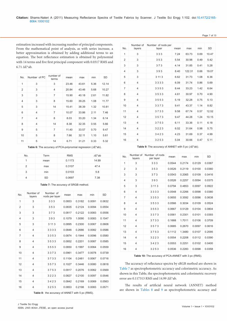
estimation increased with increasing number of principal components. From the mathematical point of analysis, as with series increase, a better approximation is obtained by adding additional terms to an equation. The best reflectance estimation is obtained by polynomial with 14 terms and five first principal component with 0.0317 RMS and 6.71 ∆E*ab.

No. Number of PC number of terms mean max min SD

1 3 3 23.46 43.61 5.36 12.14

2 3 4 20.84 43.46 5.68 10.27

3 3 7 15.90 40.18 2.61 11.82

4 3 8 15.60 39.25 1.08 11.77

5 3 14 15.41 38.39 1.32 10.81

6 4 7 10.07 33.86 2.11 7.46

7 4 8 8.03 33.20 1.34 6.14

8 4 14 8.38 32.35 0.55 5.66

9 5 7 11.40 33.57 0.70 9.47

10 5 8 7.66 32.11 1.10 5.61

11 5 14 6.71 31.21 0.33 5.32

Table 6: The accuracy of PCA-polynomial regression (∆E*ab).

No. Term RMS ∆E*ab

1 mean 0.1173 14.99

2 max 0.3107 47.4

3 min 0.0103 5.8

4 SD 0.0697 7.38

Table 7: The accuracy of SRGB method.

No. Number of layers

Number of nods per layer mean max min SD

1 3 3 3 3 0.0853 0.3182 0.0091 0.0632

2 3 3 5 3 0.0835 0.2124 0.0094 0.0554

3 3 3 7 3 0.0817 0.2122 0.0083 0.0556

4 3 3 9 3 0.1079 1.0090 0.0083 0.1547

5 3 3 11 3 0.0895 0.2300 0.0067 0.0606

6 4 3 3 3 3 0.0846 0.2686 0.0082 0.0586

7 4 3 3 5 3 0.0874 0.1944 0.0096 0.0580

8 4 3 5 3 3 0.0852 0.2201 0.0087 0.0585

9 4 3 5 5 3 0.0850 0.1997 0.0064 0.0559

10 4 3 3 7 3 0.0961 0.3477 0.0078 0.0739

11 4 3 7 3 3 0.1104 0.2481 0.0067 0.0716

12 4 3 5 7 3 0.1027 0.3446 0.0080 0.0818

13 4 3 7 5 3 0.0917 0.2076 0.0062 0.0569

14 4 3 2 2 3 0.0827 0.2100 0.0097 0.0546

15 4 3 4 2 3 0.0842 0.2169 0.0069 0.0563

16 4 3 2 5 3 0.0853 0.2198 0.0083 0.0571

Table 8: the accuracy of ANNET with 5 pc (RMS).

The accuracy of reflectance spectra by sRGB method are shown in Table 7 as spectrophotometric accuracy and colorimetric accuracy. As shown in this Table, the spectrophotometric and colorimetric recovery error are 0.117313 RMS and 14.99 ∆E*ab.

The results of artificial neural network (ANNET) method are shown in Tables 8 and 9 as spectrophotometric accuracy and

No.Number of

layersNumber of nods per

layer mean max min SD

1 3 3 3 3 7.24 63.73 0.69 10.47

2 3 3 5 3 5.54 30.98 0.49 5.42

3 3 3 7 3 4.14 31.85 0.41 5.28

4 3 3 9 3 8.40 122.31 0.66 19.07

5 3 3 11 3 6.62 31.73 1.08 6.36

6 4 3 3 3 3 6.09 31.74 0.86 5.69

7 4 3 3 5 3 8.44 33.23 1.42 6.64

8 4 3 5 3 3 4.61 30.97 0.70 4.90

9 4 3 5 5 3 5.19 32.28 0.75 5.13

10 4 3 3 7 3 9.41 43.37 1.14 8.82

11 4 3 7 3 3 9.58 67.74 0.57 12.52

12 4 3 5 7 3 9.47 44.28 1.24 10.15

13 4 3 7 5 3 6.11 33.36 0.11 6.18

14 4 3 2 2 3 6.02 31.64 0.98 5.75

15 4 3 4 2 3 4.23 31.69 0.37 4.99

16 4 3 2 5 3 5.04 30.66 0.47 5.11

Table 9: The accuracy of ANNET with 5 pc (∆E*ab).



1 3 3 3 3 0.0544 0.2174 0.0129 0.0387

2 3 3 5 3 0.0526 0.2119 0.0100 0.0360

3 3 3 7 3 0.0543 0.2065 0.0109 0.0416

4 3 3 9 3 0.0526 0.2257 0.0094 0.0375

5 3 3 11 3 0.0794 0.4853 0.0097 0.0922

6 4 3 3 3 3 0.0548 0.2266 0.0098 0.0380

7 4 3 3 5 3 0.0655 0.3592 0.0096 0.0638

8 4 3 5 3 3 0.0566 0.3034 0.0109 0.0524

9 4 3 5 5 3 0.0667 0.5129 0.0104 0.0804

10 4 3 3 7 3 0.0561 0.2301 0.0101 0.0393

11 4 3 7 3 3 0.1668 1.7011 0.0106 0.3709

12 4 3 5 7 3 0.0685 0.2670 0.0097 0.0616

13 4 3 7 5 3 0.1112 1.3480 0.0107 0.2095

14 4 3 2 2 3 0.0554 0.2208 0.0112 0.0390

15 4 3 4 2 3 0.0553 0.2251 0.0102 0.0400

16 4 3 2 5 3 0.0536 0.2283 0.0098 0.0358

Table 10: The accuracy of PCA-ANNET with 3 pc (RMS).


of 13


colorimetric accuracy, respectively. As illustrated in these tables, the spectrophotometric recovery error changed from 0.0817 to 0.1104 RMS and 4.14 to 9.58 ∆E*ab. The best reflectance estimation is obtained by neural network with one hidden layers and 7 nods with 14 terms with 0.0817 RMS and 4.14 ∆E*ab.

The results of principal component analysis and artificial neural



1 3 3 3 3 16.03 36.85 1.07 9.23

2 3 3 5 3 16.20 36.70 1.35 10.47

3 3 3 7 3 16.18 35.19 1.42 10.28

4 3 3 9 3 15.92 35.83 2.20 10.00

5 3 3 11 3 19.39 92.55 2.77 17.42

6 4 3 3 3 3 16.60 37.21 2.32 10.53

7 4 3 3 5 3 16.70 47.62 1.46 11.67

8 4 3 5 3 3 17.08 72.39 1.27 13.30

9 4 3 5 5 3 16.88 45.16 2.65 10.68

10 4 3 3 7 3 16.51 36.01 1.39 9.68

11 4 3 7 3 3 22.12 94.05 1.21 20.89

12 4 3 5 7 3 18.28 44.57 2.18 11.57

13 4 3 7 5 3 23.53 118.74 2.84 19.13

14 4 3 2 2 3 14.58 35.85 1.46 9.27

15 4 3 4 2 3 15.28 35.37 2.38 9.55

16 4 3 2 5 3 16.64 38.28 1.49 10.49

Table 11: The accuracy of PCA-ANNET with 3 pc (∆E*ab).



1 3 3 3 4 0.0360 0.1734 0.0081 0.0271

2 3 3 5 4 0.0394 0.1854 0.0081 0.0317

3 3 3 7 4 0.0396 0.2110 0.0075 0.0348

4 3 3 9 4 0.0505 0.2897 0.0076 0.0590

5 3 3 11 4 0.0530 0.2260 0.0060 0.0501

6 4 3 3 3 4 0.0444 0.2037 0.0091 0.0409

7 4 3 3 5 4 0.0453 0.2277 0.0066 0.0406

8 4 3 5 3 4 0.0457 0.2201 0.0054 0.0483

9 4 3 5 5 4 0.0426 0.2208 0.0051 0.0377

10 4 3 3 7 4 0.0566 0.3237 0.0061 0.0632

11 4 3 7 3 4 0.0553 0.3240 0.0079 0.0644

12 4 3 5 7 4 0.0614 0.3805 0.0090 0.0762

13 4 3 7 5 4 0.0697 0.4677 0.0084 0.0861

14 4 3 2 2 4 0.0379 0.1869 0.0065 0.0313

15 4 3 4 2 4 0.0361 0.1795 0.0078 0.0291

16 4 3 2 5 4 0.0460 0.2199 0.0078 0.0415


network (PCA-ANNET) method are shown in Tables 10, 12 and 14 as spectrophotometric accuracy and Tables 11, 13 and 15 as colorimetric accuracy. As illustrated in these tables, the spectrophotometric recovery error changed from 0.0297 to 0.1668RMS and 6.14 to 22.12 ∆E*ab. The best reflectance estimation is obtained by neural network with two hidden layers, respectively with 2 and 5 nods, and five principal components with 0.0297 RMS and 6.14 ∆E*ab.



1 3 3 3 4 8.65 32.44 2.07 5.66

2 3 3 5 4 8.57 32.85 2.31 6.61

3 3 3 7 4 7.68 33.22 1.05 5.52

4 3 3 9 4 9.88 55.60 1.48 9.96

5 3 3 11 4 9.00 37.08 0.67 7.66

6 4 3 3 3 4 8.06 30.37 0.24 5.55

7 4 3 3 5 4 10.75 34.91 2.08 7.51

8 4 3 5 3 4 9.44 36.45 2.06 6.50

9 4 3 5 5 4 9.76 61.14 1.63 9.78

10 4 3 3 7 4 7.26 35.44 1.20 5.49

11 4 3 7 3 4 10.57 89.06 0.80 14.73

12 4 3 5 7 4 9.14 43.64 0.99 8.32

13 4 3 7 5 4 12.65 50.84 2.24 11.78

14 4 3 2 2 4 12.74 55.46 1.45 12.39

15 4 3 4 2 4 7.81 31.73 2.05 5.26

16 4 3 2 5 4 9.25 39.44 1.87 7.71




1 3 3 3 5 0.0340 0.1767 0.0063 0.0305

2 3 3 5 5 0.0319 0.1712 0.0058 0.0299

3 3 3 7 5 0.0335 0.2099 0.0066 0.0363

4 3 3 9 5 0.0385 0.2341 0.0061 0.0470

5 3 3 11 5 0.0398 0.2142 0.0056 0.0397

6 4 3 3 3 5 0.0341 0.1713 0.0054 0.0290

7 4 3 3 5 5 0.0351 0.2002 0.0054 0.0338

8 4 3 5 3 5 0.0437 0.2306 0.0067 0.0424

9 4 3 5 5 5 0.0480 0.3465 0.0084 0.0607

10 4 3 3 7 5 0.0548 0.4766 0.0062 0.0805

11 4 3 7 3 5 0.0471 0.3205 0.0066 0.0614

12 4 3 5 7 5 0.0471 0.3205 0.0066 0.0614

13 4 3 7 5 5 0.0613 0.5755 0.0049 0.0984

14 4 3 2 2 5 0.0500 0.2786 0.0062 0.0543

15 4 3 4 2 5 0.0318 0.1721 0.0066 0.0307

16 4 3 2 5 5 0.0297 0.1780 0.0053 0.0290



of 13


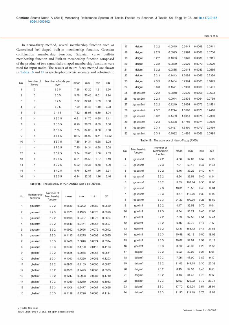
In neuro-fuzzy method, several membership function such as Generalized bell-shaped built-in membership function, Gaussian combination membership function, Gaussian curve built-in membership function and Built-in membership function composed of the product of two sigmoidally-shaped membership functions were used for input nodes. The results of neuro-fuzzy method are shown in Tables 16 and 17 as spectrophotometric accuracy and colorimetric



1 3 3 3 5 7.38 33.20 1.31 6.20

2 3 3 5 5 5.78 30.43 0.61 4.94

3 3 3 7 5 7.82 32.61 1.09 6.30

4 3 3 9 5 7.59 34.43 1.10 5.93

5 3 3 11 5 7.52 38.96 0.80 8.94

6 4 3 3 3 5 6.61 31.70 0.65 5.41

7 4 3 3 5 5 8.90 36.74 0.89 7.30

8 4 3 5 3 5 7.75 34.08 0.58 6.60

9 4 3 5 5 5 10.12 85.09 0.71 14.52

10 4 3 3 7 5 7.15 34.34 0.68 6.08

11 4 3 7 3 5 7.15 34.34 0.68 6.08

12 4 3 5 7 5 9.74 50.63 1.50 9.69

13 4 3 7 5 5 6.51 35.53 1.07 6.19

14 4 3 2 2 5 6.02 29.37 0.58 4.99

15 4 3 4 2 5 5.76 32.07 1.16 5.31

16 4 3 2 5 5 6.14 32.32 1.16 5.46


No. Membershipfunction

Number of Membership

functionmean max min SD

1 gaussmf 2 2 2 0.0839 0.2202 0.0080 0.0580

2 gaussmf 2 2 3 0.1073 0.4393 0.0070 0.0998

3 gaussmf 3 2 2 0.0899 0.2407 0.0075 0.0624

4 gaussmf 2 3 2 0.0849 0.2471 0.0064 0.0607

5 gaussmf 3 3 2 0.0962 0.5696 0.0072 0.0942

6 gaussmf 3 2 3 0.1115 0.4275 0.0093 0.0935

7 gaussmf 2 3 3 0.1486 2.6040 0.0074 0.3974

8 gaussmf 3 3 3 0.2310 2.1700 0.0116 0.4183

9 gbellmf 2 2 2 0.0825 0.2038 0.0063 0.0551

10 gbellmf 2 2 3 0.1063 0.7220 0.0088 0.1203

11 gbellmf 3 2 2 0.0957 0.4165 0.0095 0.0817

12 gbellmf 2 3 2 0.0853 0.2423 0.0063 0.0583

13 gbellmf 3 3 2 0.1247 0.9908 0.0087 0.1710

14 gbellmf 3 2 3 0.1059 0.5289 0.0065 0.1083

15 gbellmf 2 3 3 0.1006 0.2477 0.0067 0.0695

16 gbellmf 3 3 3 0.1119 0.7296 0.0063 0.1194

17 dsigmf 2 2 2 0.0815 0.2043 0.0068 0.0541

18 dsigmf 2 2 3 0.0993 0.2998 0.0068 0.0706

19 dsigmf 3 2 2 0.1033 0.5026 0.0080 0.0911

20 dsigmf 2 3 2 0.0839 0.2679 0.0073 0.0629

21 dsigmf 3 3 2 0.0835 0.2014 0.0083 0.0565

22 dsigmf 3 2 3 0.1443 1.2095 0.0065 0.2334

23 dsigmf 2 3 3 0.1464 0.7324 0.0065 0.1643

24 dsigmf 3 3 3 0.1571 2.1900 0.0069 0.3401

25 gauss2mf 2 2 2 0.0848 0.2590 0.0066 0.0603

26 gauss2mf 2 2 3 0.0914 0.3835 0.0064 0.0759

27 gauss2mf 3 2 2 0.1219 0.9454 0.0072 0.1591

28 gauss2mf 2 3 2 0.1244 1.5596 0.0071 0.2410

29 gauss2mf 3 3 2 0.1459 1.4051 0.0075 0.2360

30 gauss2mf 3 2 3 0.1328 1.1786 0.0074 0.2009

31 gauss2mf 2 3 3 0.1457 1.5360 0.0070 0.2469

32 gauss2mf 3 3 3 0.1082 0.4665 0.0066 0.0995

Table 16: The accuracy of Neuro-Fuzzy (RMS).


Number ofMembership


1 gaussmf 2 2 2 4.36 32.07 0.52 5.06

2 gaussmf 2 2 3 7.01 50.18 0.47 11.41

3 gaussmf 3 2 2 5.46 33.22 0.40 6.71

4 gaussmf 2 3 2 6.54 35.54 0.40 8.14

5 gaussmf 3 3 2 8.85 107.14 0.30 17.05

6 gaussmf 3 2 3 10.01 73.56 0.40 14.84

7 gaussmf 2 3 3 8.57 119.76 0.39 19.00

8 gaussmf 3 3 3 24.23 190.95 0.25 46.59

9 gbellmf 2 2 2 4.47 32.58 0.70 5.04

10 gbellmf 2 2 3 6.84 53.21 0.45 11.68

11 gbellmf 3 2 2 7.83 92.58 0.51 17.41

12 gbellmf 2 3 2 6.15 32.72 0.47 7.47

13 gbellmf 3 3 2 12.37 155.12 0.47 27.53

14 gbellmf 3 2 3 10.89 92.18 0.80 19.03

15 gbellmf 2 3 3 10.07 39.91 0.59 11.11

16 gbellmf 3 3 3 8.83 48.39 0.29 11.58

17 dsigmf 2 2 2 5.93 32.92 0.25 5.68

18 dsigmf 2 2 3 7.95 43.90 0.82 9.12

19 dsigmf 3 2 2 11.02 149.15 0.30 25.32

20 dsigmf 2 3 2 6.45 39.53 0.43 8.56

21 dsigmf 3 3 2 8.13 34.45 0.70 9.17

22 dsigmf 3 2 3 12.50 129.92 0.72 23.71

23 dsigmf 2 3 3 17.70 129.24 0.54 28.94

24 dsigmf 3 3 3 11.50 114.19 0.75 19.93


of 13


25 gauss2mf 2 2 2 4.70 32.97 0.50 6.18

26 gauss2mf 2 2 3 6.10 50.84 0.79 8.87

27 gauss2mf 3 2 2 12.05 128.72 0.37 25.69

28 gauss2mf 2 3 2 9.72 142.86 0.56 23.15

29 gauss2mf 3 3 2 12.68 122.72 0.50 24.54

30 gauss2mf 3 2 3 11.26 108.69 0.56 23.67

31 gauss2mf 2 3 3 12.02 93.06 0.35 22.12

32 gauss2mf 3 3 3 12.29 116.50 0.67 20.93

Table 17: The accuracy of neuro-fuzzy (∆E*ab).

Figure 10: Gaussmf membership function.




1 gaussmf 2 2 2 0.0496 0.1854 0.0107 0.0327

2 gaussmf 2 2 3 0.0619 0.5768 0.0106 0.0886

3 gaussmf 3 2 2 0.0544 0.2038 0.0094 0.0371

4 gaussmf 2 3 2 0.0518 0.1903 0.0105 0.0342

5 gaussmf 3 3 2 0.0655 0.4169 0.0104 0.0692

6 gaussmf 3 2 3 0.0585 0.2173 0.0092 0.0415

7 gaussmf 2 3 3 0.0666 0.4873 0.0100 0.0804

8 gaussmf 3 3 3 0.0877 0.4719 0.0099 0.0904

9 gbellmf 2 2 2 0.0502 0.1831 0.0098 0.0335

10 gbellmf 2 2 3 0.0608 0.4239 0.0095 0.0680

11 gbellmf 3 2 2 0.0705 0.5397 0.0098 0.0897

12 gbellmf 2 3 2 0.0530 0.1977 0.0097 0.0373

13 gbellmf 3 3 2 0.0630 0.4152 0.0111 0.0667

14 gbellmf 3 2 3 0.0535 0.2203 0.0095 0.0362

15 gbellmf 2 3 3 0.0814 0.7554 0.0094 0.1301

16 gbellmf 3 3 3 0.1183 1.2679 0.0099 0.2083

17 dsigmf 2 2 2 0.0523 0.1781 0.0095 0.0354

18 dsigmf 2 2 3 0.0625 0.3163 0.0099 0.0636

19 dsigmf 3 2 2 0.0608 0.2650 0.0110 0.0500

20 dsigmf 2 3 2 0.0511 0.1789 0.0101 0.0319

21 dsigmf 3 3 2 0.0763 0.3951 0.0104 0.0840

22 dsigmf 3 2 3 0.0790 0.4673 0.0108 0.0998

23 dsigmf 2 3 3 0.0561 0.1961 0.0122 0.0428

24 dsigmf 3 3 3 0.0766 0.4218 0.0096 0.0861

25 gauss2mf 2 2 2 0.0522 0.1852 0.0094 0.0374

26 gauss2mf 2 2 3 0.0520 0.1817 0.0104 0.0360

27 gauss2mf 3 2 2 0.0697 0.3968 0.0101 0.0822

28 gauss2mf 2 3 2 0.0534 0.1966 0.0099 0.0375

29 gauss2mf 3 3 2 0.0672 0.4074 0.0098 0.0693

30 gauss2mf 3 2 3 0.0676 0.3372 0.0105 0.0711

31 gauss2mf 2 3 3 0.0621 0.2683 0.0096 0.0555

32 gauss2mf 3 3 3 0.0746 0.3869 0.0097 0.0796

Table 18: The accuracy of PCA-Neuro-Fuzzy with 3 pc (RMS).


Number ofMembership


1 gaussmf 2 2 2 15.62 34.24 1.68 9.86

2 gaussmf 2 2 3 16.23 76.86 1.88 14.03

3 gaussmf 3 2 2 16.32 36.72 2.19 10.07

4 gaussmf 2 3 2 16.73 36.30 0.89 10.15

5 gaussmf 3 3 2 18.03 45.23 3.27 10.75

6 gaussmf 3 2 3 16.92 54.03 1.60 11.85

7 gaussmf 2 3 3 19.06 88.43 1.97 15.31

8 gaussmf 3 3 3 22.97 114.97 1.76 21.67

9 gbellmf 2 2 2 15.51 34.18 1.65 10.03

10 gbellmf 2 2 3 18.51 147.44 1.82 22.95

11 gbellmf 3 2 2 18.28 47.29 2.65 12.06

12 gbellmf 2 3 2 17.05 44.24 1.64 11.41

13 gbellmf 3 3 2 18.15 58.24 3.37 12.56

14 gbellmf 3 2 3 16.36 38.30 1.33 10.51

15 gbellmf 2 3 3 19.05 73.92 1.95 14.99

16 gbellmf 3 3 3 24.27 99.10 2.88 21.08

17 dsigmf 2 2 2 16.00 37.42 2.67 10.04

18 dsigmf 2 2 3 17.26 60.81 2.17 13.96

19 dsigmf 3 2 2 16.81 67.60 3.36 13.05

20 dsigmf 2 3 2 16.22 34.33 2.57 10.00

21 dsigmf 3 3 2 20.15 52.40 3.62 12.73

22 dsigmf 3 2 3 21.61 128.18 2.97 22.42

23 dsigmf 2 3 3 16.65 41.02 1.28 10.94

24 dsigmf 3 3 3 19.54 79.81 2.32 14.42

25 gauss2mf 2 2 2 15.98 33.64 2.30 10.17

26 gauss2mf 2 2 3 15.39 36.61 1.05 9.87

27 gauss2mf 3 2 2 17.10 46.53 1.67 11.94

28 gauss2mf 2 3 2 15.99 34.59 1.76 10.08

29 gauss2mf 3 3 2 18.65 53.71 3.64 11.66

30 gauss2mf 3 2 3 18.37 77.29 1.28 14.04


of 13


31 gauss2mf 2 3 3 17.35 43.23 1.29 12.41

32 gauss2mf 3 3 3 19.81 71.49 2.81 14.66

Table 19: the accuracy of PCA-Neuro-Fuzzy with 3 pc (∆E*ab).




1 gaussmf 2 2 2 0.0373 0.1898 0.0077 0.0315

2 gaussmf 2 2 3 0.0510 0.5749 0.0083 0.0895

3 gaussmf 3 2 2 0.0471 0.2092 0.0067 0.0453

4 gaussmf 2 3 2 0.0429 0.1908 0.0077 0.0399

5 gaussmf 3 3 2 0.0577 0.4172 0.0068 0.0781

6 gaussmf 3 2 3 0.0485 0.2175 0.0058 0.0434

7 gaussmf 2 3 3 0.0570 0.4935 0.0057 0.0849

8 gaussmf 3 3 3 0.0971 0.4820 0.0064 0.1234

9 gbellmf 2 2 2 0.0390 0.1878 0.0074 0.0350

10 gbellmf 2 2 3 0.0505 0.4180 0.0050 0.0706

11 gbellmf 3 2 2 0.0611 0.5394 0.0071 0.0924

12 gbellmf 2 3 2 0.0490 0.2982 0.0070 0.0544

13 gbellmf 3 3 2 0.0611 0.4324 0.0075 0.0793

14 gbellmf 3 2 3 0.0450 0.2194 0.0046 0.0373

15 gbellmf 2 3 3 0.0927 0.7553 0.0057 0.1440

16 gbellmf 3 3 3 0.1093 1.2668 0.0056 0.2116

17 dsigmf 2 2 2 0.0413 0.1803 0.0072 0.0361

18 dsigmf 2 2 3 0.0528 0.3157 0.0055 0.0668

19 dsigmf 3 2 2 0.0506 0.2714 0.0073 0.0521

20 dsigmf 2 3 2 0.0463 0.1881 0.0073 0.0450

21 dsigmf 3 3 2 0.0721 0.6065 0.0074 0.1104

22 dsigmf 3 2 3 0.0715 0.4695 0.0072 0.1044

23 dsigmf 2 3 3 0.0469 0.2245 0.0098 0.0498

24 dsigmf 3 3 3 0.0713 0.4075 0.0049 0.0848

25 gauss2mf 2 2 2 0.0433 0.2109 0.0076 0.0453

26 gauss2mf 2 2 3 0.0402 0.1869 0.0079 0.0359

27 gauss2mf 3 2 2 0.0591 0.3974 0.0067 0.0856

28 gauss2mf 2 3 2 0.0639 0.8142 0.0056 0.1276

29 gauss2mf 3 3 2 0.0671 0.5155 0.0058 0.1009

30 gauss2mf 3 2 3 0.0620 0.3246 0.0074 0.0804

31 gauss2mf 2 3 3 0.0580 0.3399 0.0059 0.0729

32 gauss2mf 3 3 3 0.0672 0.3917 0.0055 0.0811



Number ofMembership


1 gaussmf 2 2 2 7.80 33.74 1.06 6.13

2 gaussmf 2 2 3 9.37 78.73 2.14 12.27

3 gaussmf 3 2 2 10.78 51.23 0.79 9.68

4 gaussmf 2 3 2 10.15 36.33 1.41 8.82

5 gaussmf 3 3 2 11.49 46.56 0.64 10.13

6 gaussmf 3 2 3 10.22 59.38 2.04 10.30

7 gaussmf 2 3 3 10.34 82.43 1.35 13.36

8 gaussmf 3 3 3 17.95 118.35 1.65 23.68

9 gbellmf 2 2 2 8.07 31.25 1.83 5.83

10 gbellmf 2 2 3 12.47 147.07 2.32 22.71

11 gbellmf 3 2 2 12.27 48.41 1.02 11.05

12 gbellmf 2 3 2 11.36 39.60 1.52 9.98

13 gbellmf 3 3 2 14.14 65.57 1.67 14.90

14 gbellmf 3 2 3 9.37 38.24 2.64 6.65

15 gbellmf 2 3 3 14.25 73.96 0.61 17.34

16 gbellmf 3 3 3 16.70 96.41 1.03 21.13

17 dsigmf 2 2 2 9.83 30.28 2.95 6.35

18 dsigmf 2 2 3 11.44 80.73 1.73 15.76

19 dsigmf 3 2 2 10.85 79.29 1.28 12.86

20 dsigmf 2 3 2 10.41 39.18 1.10 8.56

21 dsigmf 3 3 2 14.76 84.23 1.32 15.56

22 dsigmf 3 2 3 16.45 128.37 0.96 23.90

23 dsigmf 2 3 3 9.81 36.57 1.91 7.73

24 dsigmf 3 3 3 13.87 85.98 1.94 14.23

25 gauss2mf 2 2 2 9.46 32.61 1.81 7.08

26 gauss2mf 2 2 3 9.33 37.90 2.21 7.97

27 gauss2mf 3 2 2 12.36 63.68 0.49 13.68

28 gauss2mf 2 3 2 12.90 128.67 0.80 20.13

29 gauss2mf 3 3 2 14.64 95.00 0.78 19.43

30 gauss2mf 3 2 3 11.90 88.75 1.76 14.96

31 gauss2mf 2 3 3 10.42 39.03 0.97 7.96

32 gauss2mf 3 3 3 13.21 49.98 1.03 10.71

Table 21: the accuracy of PCA-Neuro-Fuzzy with 4 pc (∆E*ab).




1 gaussmf 2 2 2 0.0328 0.1899 0.0061 0.0322

2 gaussmf 2 2 3 0.0478 0.5838 0.0069 0.0919

3 gaussmf 3 2 2 0.0447 0.2377 0.0053 0.0503

4 gaussmf 2 3 2 0.0406 0.1995 0.0054 0.0442

5 gaussmf 3 3 2 0.0551 0.4170 0.0052 0.0799

6 gaussmf 3 2 3 0.0500 0.3437 0.0051 0.0633

7 gaussmf 2 3 3 0.0570 0.5828 0.0050 0.0997

8 gaussmf 3 3 3 0.0953 0.4855 0.0060 0.1252

9 gbellmf 2 2 2 0.0349 0.1880 0.0054 0.0366

10 gbellmf 2 2 3 0.0473 0.4183 0.0044 0.0717


of 13


11 gbellmf 3 2 2 0.0591 0.5538 0.0060 0.0959

12 gbellmf 2 3 2 0.0473 0.3180 0.0063 0.0593

13 gbellmf 3 3 2 0.0583 0.4403 0.0055 0.0809

14 gbellmf 3 2 3 0.0420 0.2222 0.0045 0.0396

15 gbellmf 2 3 3 0.0919 0.8236 0.0051 0.1536

16 gbellmf 3 3 3 0.1067 1.2668 0.0049 0.2131

17 dsigmf 2 2 2 0.0386 0.2147 0.0069 0.0435

18 dsigmf 2 2 3 0.0502 0.3321 0.0053 0.0695

19 dsigmf 3 2 2 0.0482 0.2974 0.0048 0.0571

20 dsigmf 2 3 2 0.0516 0.3358 0.0059 0.0677

21 dsigmf 3 3 2 0.0690 0.6069 0.0054 0.1087

22 dsigmf 3 2 3 0.0722 0.4776 0.0051 0.1096

23 dsigmf 2 3 3 0.0507 0.2789 0.0082 0.0605

24 dsigmf 3 3 3 0.0688 0.4061 0.0041 0.0865

25 gauss2mf 2 2 2 0.0391 0.2067 0.0062 0.0458

26 gauss2mf 2 2 3 0.0368 0.1874 0.0069 0.0402

27 gauss2mf 3 2 2 0.0622 0.5753 0.0059 0.1086

28 gauss2mf 2 3 2 0.0601 0.7787 0.0048 0.1235

29 gauss2mf 3 3 2 0.0655 0.5060 0.0065 0.1005

30 gauss2mf 3 2 3 0.0602 0.3395 0.0056 0.0837

31 gauss2mf 2 3 3 0.0556 0.3402 0.0056 0.0776

32 gauss2mf 3 3 3 0.0640 0.3569 0.0050 0.0792



Number ofMembership


1 gaussmf 2 2 2 6.42 32.54 1.75 5.58

2 gaussmf 2 2 3 8.59 73.39 1.48 11.64

3 gaussmf 3 2 2 9.17 35.90 1.23 7.95

4 gaussmf 2 3 2 8.98 36.79 0.64 9.59

5 gaussmf 3 3 2 10.24 48.38 0.43 11.04

6 gaussmf 3 2 3 9.50 74.58 1.10 12.74

7 gaussmf 2 3 3 8.93 88.18 0.98 14.01

8 gaussmf 3 3 3 17.26 110.00 0.89 23.15

9 gbellmf 2 2 2 7.21 30.02 0.89 6.01

10 gbellmf 2 2 3 11.46 142.50 1.02 22.40

11 gbellmf 3 2 2 11.07 46.93 0.98 11.41

12 gbellmf 2 3 2 9.76 33.37 1.48 10.00

13 gbellmf 3 3 2 11.97 59.68 0.53 14.21

14 gbellmf 3 2 3 8.73 34.76 1.12 6.29

15 gbellmf 2 3 3 14.55 79.43 1.93 17.45

16 gbellmf 3 3 3 15.39 96.85 1.43 21.36

17 dsigmf 2 2 2 8.54 29.02 1.93 6.68

18 dsigmf 2 2 3 11.33 79.88 1.88 15.26

19 dsigmf 3 2 2 9.47 82.16 0.65 13.36

20 dsigmf 2 3 2 6.81 30.58 1.24 6.39

21 dsigmf 3 3 2 13.24 86.24 1.12 16.18

22 dsigmf 3 2 3 16.14 132.24 0.89 26.81

23 dsigmf 2 3 3 9.95 43.43 1.29 9.00

24 dsigmf 3 3 3 12.80 92.64 1.38 15.27

25 gauss2mf 2 2 2 8.23 31.30 1.72 6.85

26 gauss2mf 2 2 3 8.03 41.15 0.83 7.88

27 gauss2mf 3 2 2 11.07 77.86 0.67 15.11

28 gauss2mf 2 3 2 11.57 128.39 0.75 20.18

29 gauss2mf 3 3 2 12.97 92.11 0.64 17.16

30 gauss2mf 3 2 3 10.88 79.31 1.22 13.85

31 gauss2mf 2 3 3 9.22 35.75 0.84 7.49

32 gauss2mf 3 3 3 11.71 50.03 1.11 11.54

Table 23: The accuracy of PCA-Neuro-Fuzzy with 5 pc (∆E*ab).

accuracy, respectively. As illustrated in these Tables, the reflectance recovery error changed from 0.0815 to 0.2310 RMS and 4.36 to 24.23 ∆E*ab. The best reflectance estimation is obtained by neuro-fuzzy with Gaussian curve built-in membership function (gaussmf) (Figure 10) with 14 terms with 0.0839 RMS and 4.36 ∆E*ab.

In PCA-neuro-fuzzy method, several membership function such as Generalized bell-shaped built-in membership function, Gaussian combination membership function, Gaussian curve built-in membership function and Built-in membership function composed of the product of two sigmoidally-shaped membership functions were used for input nodes. The results of neuro-fuzzy method are shown in Tables 18, 20 and 22 as spectrophotometric accuracy and Tables 19, 21 and 23 as colorimetric accuracy. As illustrated in these tables, the reflectance recovery error changed from 0.0328 to 0.1183 RMS and 6.42 to 24.27∆E*ab. The best reflectance estimation is obtained by neuro-fuzzy with 2 Gaussian curve built-in membership function (gaussmf) for each input and 5 principal components with 0.0328 RMS and 6.42 ∆E*ab.

Conclusions This article explained a numerical method based on principal

component analysis, polynomial regression, neural network and neuro-fuzzy techniques to measure the reflectance spectra by scanner.

In polynomial method, estimation error is 0.0820 RMS and 5.79 ∆E*ab. The reflectance estimation error in PCA-polynomial method is 0.0317 RMS and 6.71 ∆E*ab. In sRGB method, the estimation error is 0.1173 RMS and 14.99 ∆E*ab. The reflectance estimation error of neural network method is 0.0817 RMS and 4.14 ∆E*ab. In PCA- ANNET method, the estimation error is 0.0297 RMS and 6.14 ∆E*ab. The reflectance estimation error of neuro-fuzzy method is 0.0839 RMS and 4.36 ∆E*ab. In PCA-neuro-fuzzy method error is 0.0328 RMS and 6.42 ∆E*ab. Obtained results indicate that the recovery error decreases with increase number of principal component and number of terms in a polynomial. Also, application of principal component increase accuracy of reflectance measurement. The reflectance estimation performance of PCA- ANNET method is better than others.


of 13


References

1. Kang HR (1992) Color Scanner Calibration. Journal of Imaging Science and Technology 36: 162-170.

2. Andersson M (2004) Topics in Color Measurement. Linköping Studies in Science and Technology, Licentiate Thesis No. 1143.

3. Hung PC (1991) Colorimetric Calibration for Scanners and Media. Proceedings of SPIE. Camera and Input Scanner Systems.

4. Vrhel MJ, HJ Trussell (1448) Color Device Calibration: a Mathematical Formulation. IEEE Transactions on Image Processing 8: 1796 - 1806.

5. Stephen Viggiano JA, C Jeffrey Wang (1993) A Novel Method For Colorimetric Calibration of Color Digitizing Scanners.TAGA Proceedings.

6. Vrhel MJ, Trussell HJ (1999) Color Device Calibration: A Mathematical Formulation.IEEE Transactions on Image Processing.

7. Emmel P, Hersch RD (2000) Colour Calibration for Colour Reproduction.ISCAS2000 - IEEE International Symposium on Circuits and Systems, Geneva, Switzerland.

8. Hardeberg JY (2000) Acquisition and reproduction of colour images: colorimetric and multispectral approaches.

9. Murakami Y, Obi T, Yamaguchi M, Ohyama N, Komiya Y(2001) Spectral refectance estimation from multi-band image using color chart. Optics Communications 188: 47-54.

10. Morovic P, Finlayson D (2006) Metamer-set-based approach to estimating surface reflectance from camera RGB.OSA A 23: 1814-1822.

11. Shi M, Healey G (2002) Using reflectance models for color scanner calibration. JOSA A, 19: 645-656.

12. Morovic P, Finlayson G D (2005) Reflectance estimation with uncertainty. AIC Colour 05 - 10th Congress of the International Colour Association.

13. Westland S, Ripamonti C (2004) Computational Colour Science Using Matlab. John Wiley & Sons, Ltd, England.

14. Shlens J (2003) A tutorial on principal component analyzing.

15. Smith D (2002) A tutorial on Principal Components Analysis.

16. Jolliffe I T (2002) Principal component Analysis, Second edition.

17. Ansari K, Amirshahi S H, Moradian S (2006) Recovery of reflectance spectra from CIE tristimulus values using a progressive database selection technique. Color Technol 122: 128-134.

18. Fairman HS, Brill M H (2004) The Principal Components of Reflectance .Color Research and Application 29: 104–110.

19. Tzeng DY, Berns RS (2005) A Review of Principal Component Analysis and Its Applications to Color Technology. Color Research and Application 30: 84–98.

20. Dupont D (2002) Study of the Reconstruction of Reflectance Curves Based on Tristimulus Values: Comparison of Methods of Optimization.Color Research & Application 27: 88-99.

21. Rumelhart GE, Hilton GE, Williams RG (1986) Learning Internal Representationby Error Propagation, in: Parallel Distributed Processing.

22. Torkamani-Azar F (1995) Comparative studies of Diffusion Equation Image Recovery Methods with an Improved Neural Network Embedded Technique.

23. Torkamani-Azar F (1996) A Modified Back Propagation Algorithm. Second Annual Computer Society of Iran Conference, Tehran.

24. Demuth H, Beale M (2001) Neural network toolbox for use with MATLAB.

25. Marjoniemi M, Mantysalo E (1997) Neuro-Fuzzy Modeling of Spectroscopic Data. Part A: Modelling of dye solutions. JSDC 113:13-17.

26. Jang JSR (1993) ANFIS: Adaptive-network-based fuzzy Inference System. IEEE Trans. On Sys. Man. Cyb.

27. Nariman-Zadeh N, Darvizeh A (2001) Design of Fuzzy System for the Modelingof Explosive Cutting Process of Plates Using Singular Value Decomposition. WSES 2001 Conf. On fuzzy sets and fuzzy systems, Spain.

http://cat.inist.fr/?aModele=afficheN&cpsidt=5620249

http://cat.inist.fr/?aModele=afficheN&cpsidt=5620249

http://ieeexplore.ieee.org/xpl/freeabs_all.jsp?arnumber=806624

http://ieeexplore.ieee.org/xpl/freeabs_all.jsp?arnumber=806624

http://books.google.co.in/books?hl=en&lr=&id=e2umTIdI2u4C&oi=fnd&pg=PR1&dq=Acquisition+and+reproduction+of+colour+images:+colorimetric+and+multispectral+approaches.++&ots=KFPg6rxNzm&sig=CjAyolOGtrQ_6yF4v8uFcV_p2e8#v=onepage&q=Acquisition and reproducti

http://books.google.co.in/books?hl=en&lr=&id=e2umTIdI2u4C&oi=fnd&pg=PR1&dq=Acquisition+and+reproduction+of+colour+images:+colorimetric+and+multispectral+approaches.++&ots=KFPg6rxNzm&sig=CjAyolOGtrQ_6yF4v8uFcV_p2e8#v=onepage&q=Acquisition and reproducti

http://www.sciencedirect.com/science/article/pii/S0030401800011317



http://www.opticsinfobase.org/abstract.cfm?id=90841




http://www.cs.cmu.edu/~elaw/papers/pca.pdf

http://onlinelibrary.wiley.com/doi/10.1111/j.1478-4408.2006.00019.x/full



http://onlinelibrary.wiley.com/doi/10.1002/col.10230/abstract







http://en.scientificcommons.org/36109822

http://en.scientificcommons.org/36109822

http://citeseerx.ist.psu.edu/viewdoc/summary?doi=10.1.1.27.9069

http://onlinelibrary.wiley.com/doi/10.1111/j.1478-4408.1997.tb01840.x/abstract

http://onlinelibrary.wiley.com/doi/10.1111/j.1478-4408.1997.tb01840.x/abstract

textile science & engineering - omics international device has a different gamut and its own...

Documents