Teukolsky Master Equation: De Rham wave equation

for the gravitational and electromagnetic fields in

vacuum

Donato Bini∗,†, Christian Cherubini],†, Robert T. Jantzen¶,†,

and Remo Ruffini[,†

∗ Istituto per le Applicazioni del Calcolo, “M. Picone,” C.N.R.,

I– 00161 Rome, Italy.† I.C.R.A., Univ. of Rome, I–00185 Roma, Italy.

¶ Dept. of Math. Sciences, Villanova Univ., Villanova, PA 19085, USA.] Dip. di Fisica “E.R. Caianiello,” Univ. di Salerno, I–84081, Italy.

[ Physics Dept., Univ. of Rome, I–00185 Roma, Italy.

Abstract

A new version of the Teukolksy Master Equation, describing any massless field of

different spin s = 1/2, 1, 3/2, 2 in the Kerr black hole, is presented here in the form

of a wave equation containing additional curvature terms. These results suggest a re-

lation between curvature perturbation theory in general relativity and the exact wave

equations satisfied by the Weyl and the Maxwell tensors, known in the literature as the

de Rham-Lichnerowicz Laplacian equations. We discuss these Laplacians both in the

Newman-Penrose formalism and in the Geroch-Held-Penrose variant for an arbitrary

vacuum spacetime. Perturbative expansion of these wave equations results in a recur-

sive scheme valid for higher orders. This approach, apart from the obvious implications

for the gravitational and electromagnetic wave propagation on a curved spacetime, ex-

plains and extends the results in the literature for perturbative analysis by clarifying

their true origins in the exact theory.

1 typeset using PTPTEX.sty <ver.1.0>

§1. Introduction

In recent years there has been considerable interest in perturbations of the gravitational

field and in other spin s massless test fields (s = 1/2, 1, 3/2, 2) imposed on a gravitational

background (especially on a black hole background, which is of particular interest for study-

ing features of gravitational collapse and consequent gravitational wave emission). The

approaches to perturbations existing in the literature can be divided essentially into two

classes: 1) metric perturbations and 2) curvature perturbations.

Pioneering work in the first class was done by Regge, Wheeler and Zerilli, who produced

important results for spherically symmetric black holes 1) - 3) by decomposing the metric

perturbations into multipoles which satisfy a set of (linearized) equations 4) - 9). However, a)

perturbing the metric components written with respect to some coordinate system is not

a “gauge invariant” procedure as pointed out by Stewart and Walker 10) and b) apart from

spherically symmetric background solutions, this approach does not seem to be very useful.

Working in the second class, i.e., perturbing directly the components of the curvature

tensor, one can use frames adapted to the null principal directions of the Weyl tensor of the

background spacetime: this allows special simplifications (even partial decoupling) of the

equations themselves. However, this approach has problems too: perturbing the components

of the curvature tensor with respect to some special adapted frame is not a “tetrad invariant”

procedure and one must add this difficulty to that of the gauge invariance which is still

present.

The “state of the art” regarding curvature perturbations is still represented by the work

of Teukolsky 11) (in the context of the Newman-Penrose formalism 12), NP in the following),

which partially received its mathematical foundation by Stewart and Walker 10) and was

subjected to some extensions by other authors 13) - 16), 30) - 33). Very recently, a gauge-invariant

second-order perturbation study for a type D vacuum geometry was initiated by Lousto and

Campanelli 35), also stimulated by relevant results concerning the second order perturbations

of a Schwarzschild black hole 36).

We introduce a new form of the Teukolksy Master Equation, closer to a “generalized

Klein Gordon” equation. This allows us to investigate exact wave equations on a general

vacuum spacetime: the de Rham-Lichnerowicz equation satisfied by the Riemann tensor

as well as the ordinary de Rham equation satisfied by the Maxwell tensor in a test field

approximation. All the results are formulated for tensor components with respect to any

frame and then specialized to the Newman-Penrose formalism and to its further extension,

the GHP formalism, introduced by Geroch, Held and Penrose 33). Starting from the exact

equations for the Riemann and Maxwell tensor components, it is easy to give a unified and

2

complete picture of the existing theory of perturbations to any order, framing all the known

results (which are scattered in many different formalisms) in a more general form. In type

D spacetimes all the known results, including those of Teukolsky 11), Stewart and Walker 10)

and Lousto and Campanelli 35) are easily recovered and discussed. Finally, some remarks are

given about how this approach can be generalized to half-integer spin test fields as well as

to the case of nonvacuum spacetimes.

§2. The Newman-Penrose formalism: a brief review

In this article we introduce the Newman-Penrose form of the generalized de Rham wave

operator for the Weyl, Riemann and Maxwell tensors. To accomplish this, it is first nec-

essary to specify all the formalism conventions: we will follow exactly the notations of

Chandrasekhar 37). For the sake of completeness we recall here some details.

A Newman-Penrose frame is defined by four complex null vector fields e1 = l, e2 = n,

e3 = m, e4 = m∗, satisfying the relations

l ·m = l ·m∗ = n ·m = n ·m∗ = 0,

l · l = n · n = m ·m = m∗ ·m∗ = 0,

l · n = 1, m ·m∗ = −1,

(2.1)

so that the components of the metric tensor in this frame are

ηab = ηab =

0 1 0 0

1 0 0 0

0 0 0 −1

0 0 −1 0

. (2.2)

With an abuse of notation (not distinguishing vectors and 1-forms) the dual frame is

e1 = n = e2 , e2 = l = e1 ,

e3 = −m∗ = −e4, e4 = −m = −e3 . (2.3)

The basis vectors, thought of as directional derivative operators when acting on scalars, are

denoted by

e1 = e2 = D, e2 = e1 = ∆ ,

e3 = −e4 = δ, e4 = −e3 = δ∗, (2.4)

3

and the 12 complex spin coefficents are introduced through the following linear combinations

of the 24 Ricci rotation (connection) coefficents γcab = ec · ∇ebea = −γacb

κ = γ311, ρ = γ314, ε =1

2(γ211 + γ341),

σ = γ313, µ = γ243, γ =1

2(γ212 + γ342),

λ = γ244, τ = γ312, α =1

2(γ214 + γ344),

ν = γ242, π = γ241, β =1

2(γ213 + γ343) .

(2.5)

As a general rule, complex conjugation of null frame components is equivalent to interchang-

ing the indices 3 and 4. Using this prescription the inverse relations of (2.5) are

γ121 = −(ε + ε∗), γ122 = −(γ + γ∗), γ123 = −(β + α∗), γ124 = −(α + β∗),

γ131 = −κ, γ132 = −τ, γ133 = −σ, γ134 = −ρ,γ141 = −κ∗, γ142 = −τ ∗, γ143 = −ρ∗, γ144 = −σ∗,γ231 = π∗, γ232 = ν∗, γ233 = λ∗, γ234 = µ∗,

γ241 = π, γ242 = ν, γ243 = µ, γ244 = λ,

γ341 = (ε− ε∗), γ342 = γ − γ∗, γ343 = β − α∗, γ344 = α− β∗ .

(2.6)

The commutation rules (Lie brackets) [ea, eb] = Ccabec reduce to

[∆,D] =(γ + γ∗)D + (ε+ ε∗)∆− (τ ∗ + π)δ − (τ + π∗)δ∗,

[δ,D] =(α∗ + β − π∗)D + κ∆− (ρ∗ + ε− ε∗)δ − σδ∗,[δ,∆] =− ν∗D + (τ − α∗ − β)∆+ (µ− γ + γ∗)δ + λ∗δ∗,

[δ∗, δ] =(µ∗ − µ)D + (ρ∗ − ρ)∆ + (α− β∗)δ + (β − α∗)δ∗.

(2.7)

The 10 independent components Cabcd of the Weyl tensor are represented by 5 complex

scalars in the Newman-Penrose formalism

Ψ0 =− C1313 =− Cabcd lamblcmd,

Ψ1 =− C1213 =− Cabcd lanblcmd,

Ψ2 =− C1342 =− Cabcd lambm∗cnd,

Ψ3 =− C1242 =− Cabcd lanbm∗cnd,

Ψ4 =− C2424 =− Cabcd nam∗bncm∗d ,

(2.8)

4

with the additional properties

C1334 =C1231 = Ψ1, C1241 =C1443 = Ψ ∗1 ,

C1212 =C3434 = −(Ψ2 + Ψ ∗2 ), C1234 =(Ψ2 − Ψ ∗

2 ),

C2443 =− C1242 = Ψ3, C1232 =C2343 = −Ψ ∗3 ,

(2.9)

and C1314 = C2324 = C1332 = C1442 = 0. Analogously, the 10 independent components Rab of

the Ricci tensor are represented by the following (four real and three independent complex)

scalars, packaged in their tracefree (Φ) and pure trace (Λ) parts

Φ00 =− 1

2R11, Φ22 =− 1

2R22,

Φ02 =− 1

2R33, Φ20 =− 1

2R44,

Φ11 =− 1

4(R12 +R34), Φ01 =− 1

2R13,

Φ10 =− 1

2R14, Φ12 =− 1

2R23,

Φ21 =− 1

2R24, Λ =

1

24R = − 1

12(R12 − R34) .

(2.10)

The components Rabcd of the Riemann tensor are then related to the Weyl and Ricci tensors

by:

R1212 =− Ψ2 − Ψ ∗2 − 2Φ11 − 10Λ, R1324 =Ψ2 + 2Λ,

R1234 =Ψ2 − Ψ ∗2 , R3434 =− Ψ2 − Ψ ∗

2 + 2Φ11 − 10Λ,

R1313 =− Ψ0, R2323 =− Ψ ∗4 ,

R1314 =− Φ00, R2324 =− Φ22,

R3132 =Φ02, R1213 =− Ψ1 − Φ01,

R1334 =− Ψ ∗1 − Φ01, R1223 =Ψ ∗

3 + Φ12,

R2334 =− Ψ ∗3 − Φ12 ,

(2.11)

with the additional complex conjugate relations obtained by interchanging the indices 3 and

4.

The six independent components Fab of the (antisymmetric) Maxwell tensor are repre-

sented by the three complex scalars

φ0 = F13 , φ1 =1

2(F12 + F43) , φ2 = F42 , (2.12)

5

with the inverse relations

Fab =

0 φ∗1 + φ1 φ0 φ∗0

−φ∗1 − φ1 0 −φ∗2 −φ2

−φ0 φ∗2 0 φ∗1 − φ1

−φ∗0 φ2 −φ∗1 + φ1 0

. (2.13)

Finally the Ricci and the Bianchi identities are given explicitly in the book of Chan-

drasekhar 37) (section 1.8). Here they will be referred to according to the components of the

Riemann tensor which give rise to the corresponding equation: [Rabcd] stands for the Ricci

identity associated with Rabcd and Rab[cd|e] = 0 for the Bianchi identities.

Exchange of l↔ n, m↔m∗ in the various Newman-Penrose quantities implies

D = lµ∂µl↔n←→ nµ∂µ

m↔m∗←→ nµ∂µ = ∆,

δ = mµ∂µl↔n←→ mµ∂µ

m↔m∗←→ m∗µ∂µ = δ∗,

(2.14)

κ = γ311l↔n←→ γ322

m↔m∗←→ γ422 = −γ242 = −ν,

τ = γ312l↔n←→ γ321

m↔m∗←→ γ421 = −γ241 = −π,

σ = γ313l↔n←→ γ323

m↔m∗←→ γ424 = −γ244 = −λ,

ρ = γ314l↔n←→ γ324

m↔m∗←→ γ423 = −γ243 = −µ,

(2.15)

ε =1

2(γ211 + γ341)

l↔n←→ 1

2(γ122 + γ342)

m↔m∗←→ 1

2(γ122 + γ432) = −γ,

α =1

2(γ214 + γ344)

l↔n←→1

2(γ124 + γ344)

m↔m∗←→ 1

2(γ123 + γ433) = −β,

(2.16)

Ψ0 = −C1313l↔n←→ − C2323

m↔m∗←→ −C2424 = Ψ4,

Ψ1 = −C1213l↔n←→ − C2123

m↔m∗←→ −C2124 = −C1242 = Ψ3,

Ψ2 = −C1342l↔n←→ − C2341

m↔m∗←→ −C2431 = −C1342 = Ψ2 .

(2.17)

φ0 = F13l↔n←→ F23

m↔m∗←→ F24 = −φ2,

φ1 =1

2(F12 + F43)

l↔n←→ 1

2(F21 + F43)

m↔m∗←→ 1

2(F21 + F34) = −φ1.

(2.18)

These operations are useful since they may be used to extend a given component calcu-

lation to other components.

6

§3. NP gravitational perturbations

The study of perturbations of the various fields in the NP formalism is achieved by

splitting all the relevant quantities in the form l = lA + lB + ..., Ψ4 = ΨA4 + ΨB

4 + ..., σ =

σA +σB + ...,D = DA +DB + ..., etc., where the A terms are the background and the B’s are

small perturbations etc. The full set of perturbative equations is obtained inserting first of

all these splitted quanties in the basic equations of the theory (Ricci and Bianchi identities,

Maxwell, Dirac, Rarita-Schwinger equations etc..) and keeping only first order terms. After

some “ad hoc” algebraic manipulations, which generate second order differential relations,

one usually obtains second order coupled linear PDE for the curvature quantities. However

for some very special spacetimes, as for Petrov type D ones (i.e. Kerr metric), some PDE’s

are decoulpled. In the following we’ll present an example of this procedure, applied to a

generic vacuum type D metric, for which it follows that:

ΨA0 = ΨA

1 = ΨA3 = ΨA

4 = 0 (3.1)

κA = σA = νA = λA = 0 . (3.2)

We start from the exact NP relations: 11):

(δ∗ − 4α+ π)Ψ0 − (D − 4ρ− 2ε)Ψ1 − 3κΨ2 = (δ + π∗ − 2α∗ − 2β)Φ00

−(D − 2ε− 2ρ∗)Φ01 + 2σΦ10 − 2κΦ11 − κ∗Φ02 (3.3)

(∆− 4γ + µ)Ψ0 − (δ − 4τ − 2β)Ψ1 − 3σΨ2 = (δ + 2π∗ − 2β)Φ01

−(D − 2ε+ 2ε∗ − ρ∗)Φ02 − λ∗Φ00 + 2σΦ11 − 2κΦ12 (3.4)

(D − ρ− ρ∗ − 3ε+ ε∗)σ − (δ − τ + π∗ − α∗ − 3β)κ− Ψ0 = 0 . (3.5)

In the tetrad language, (3.3) represents R13[13|4] = 0, (3.4) represents R13[13|2] = 0 (they

are two components of the Bianchi identities) and (3.5) is the Ricci identity component

R1313 = 0. In this notation we have:

Φ00 ≡ −1

2Rµν l

µlν = 4πTµν lµlν ≡ 4πTll (3.6)

and in the same sense one has to look at the other Φij. Obviously, in (3.6) π is not a spin

coefficient but it is the usual mathematical constant coming from the right hand side of

the Einstein equations. Because we are in vacuo, after the perturbative expansion, in these

7

relations we have that ΨA0 , ΨA

1 , σA , κA, Λ and all the ΦAnm are zero and consequently we

get:

(δ∗ − 4α + π)AΨB0 − (D − 4ρ− 2ε)AΨB

1 − 3κBΨA2 =

4π[(δ + π∗ − 2α∗ − 2β)ATBll − (D − 2ε− 2ρ∗)ATB

lm](3.7)

(∆− 4γ + µ)AΨB0 − (δ − 4τ − 2β)AΨB

1 − 3σBΨA2 =

4π[(δ + 2π∗ − 2β)ATBlm − (D − 2ε+ 2ε∗ − ρ∗)ATB

mm](3.8)

(D − ρ− ρ∗ − 3ε+ ε∗)AσB − (δ − τ + π∗ − α∗ − 3β)AκB − ΨB0 = 0 . (3.9)

In the following, we’ll obmit the A superscript for the background quantities to simplify the

notation. The type D background metric satisfy the relations:

DΨ2 = 3ρΨ2 (3.10)

δΨ2 = 3τΨ2 , (3.11)

so multiplying (3.9) by Ψ2 and taking into account that

Ψ2DσB = D(Ψ2σ

B)− σBDΨ2 = D(Ψ2σB)− σB3ρΨ2 (3.12)

Ψ2δκB = δ(Ψ2κ

B)− κBδΨ2 = δ(Ψ2κB)− κB3τΨ2 (3.13)

we obtain the relation:

(D − 3ε+ ε∗ − 4ρ− ρ∗)Ψ2σB − (δ + π∗ − α∗ − 3β − 4τ)Ψ2κ

B − ΨB0 Ψ2 = 0. (3.14)

We have now to eliminate ΨB1 from the eqns (3.7) and (3.8). To accomplish this task we use

the commuting relation found by Teukolsky and valid for any type D metric:

[D − (p + 1)ε+ ε∗ + qρ− ρ∗](δ − pβ + qτ)

−[δ − (p + 1)β − α∗ + π∗ + qτ ](D − pε+ qρ) = 0 (3.15)

where p and q are two generic constants. We apply now (D−3ε+ ε∗−4ρ−ρ∗) on (3.8) and

(δ + π∗ − α∗ − 3β − 4τ) on (3.7) and we subtract the two resulting equations. We can now

use (3.15) with the choice p = 2 and q = −4 to eliminate the ΨB1 term. The combination σB

and κB remained is exactly the same present in eq. (3.14), and consequently these quantities

can be eliminate in favor of the Ψ2ΨB0 term. The final equation is:

[(D − 3ε+ ε∗ − 4ρ− ρ∗)(∆ + µ− 4γ)− (δ + π∗ − α∗ − 3β − 4τ)

× (δ∗ + π − 4α)− 3Ψ2]ΨB0 = 4πT0 (3.16)

8

where we have posed:

T0 = (δ + π∗ − α∗ − 3β − 4τ)[(D − 2ε− 2ρ∗)TBlm − (δ + π∗ − 2α∗ − 2β)TB

ll ]

+ (D − 3ε+ ε∗ − 4ρ− ρ∗)[(δ + 2π∗ − 2β)TBlm − (D − 2ε + 2ε∗ − ρ∗)TB

mm] .

(3.17)

In the same way one can build the other relations to perform the perturbative analisys

of a type D vacuum spacetime. We point out that the same technique can be applied to

the NP Maxwell equations to decouple them as well to the neutrino and Rarita-Schwinger

ones 11), 25) It is important to stress that this perturbative theory has a purely “algebraic and

manipulative” nature, without taking into account the geometry underlying the problem.

In the following we’ll give to this subject a new geometrical meaning, framing it into the

context of the field theory. But to accomplish this task we have to adapt the previous studies

to the Kerr solution, which describes a rotating black hole of specific angular momentum a

and mass M , with the condition of flat spacetime at infinity.

§4. The Teukolsky Master Equation

The Kerr solution in Boyer-Lindquist coordinates is given by 21):

ds2 =(

1− 2Mr

Σ

)dt2 +

4aMr sin2 θ

Σdtdφ− Σ

∆dr2

−Σdθ2 − 2Mr

[r2 + a2 +

a2 sin2 θ

Σ

]sin2 θdφ2 (4.1)

where as usual:

∆ ≡ r2 − 2Mr + a2, Σ ≡ r2 + a2 cos2 θ (4.2)

For any Petrov type D metric, and in particular for the Kerr solution, simplifications occur

working in a tetrad adapted to the two repeated principal null directions of the corresponding

Weyl tensor. In the NP formalism the following quantities 17) completely describe the Kerr

solution (in this section we use the label A over some quantities in view of a perturbative

analysis, as will be clear in the following). The Kinnersley tetrad 18):

(lµ)A =1

∆[r2 + a2, ∆, 0, a]

(nµ)A =1

2Σ[r2 + a2,−∆, 0, a] (4.3)

(mµ)A=1√

2(r + ia cos θ)[ia sin θ, 0, 1,

i

sin θ] ,

9

with the 4th tetrad vector being (m∗µ)A, the complex conjugate of (mµ)A. The Weyl tensor

is represented by:

ΨA0 = ΨA

1 = ΨA3 = ΨA

4 = 0

(4.4)

ΨA2 = M(ρA)3

while the Ricci tensor and the curvature scalar are identically zero because of the vacuum

spacetime. The spin coefficents are given by:

κA = σA = λA = νA = εA = 0 ,

ρA =−1

(r − ia cos θ), τA =

−iaρAρ∗A sin θ√2

,

βA =−ρ∗A cot θ

2√

2, πA =

ia(ρA)2 sin θ√2

, (4.5)

µA =(ρA)2ρ∗A∆

2, γA = µA +

ρAρ∗A(r −M)

2,

αA = πA − β∗A .

It is a relevant result that all the massless (non trivial) perturbations of different spin of

the Kerr metric are included into the Teukolsky Master Equation (TME) 11) which has the

following form (π is the mathematical constant):

[(r2 + a2)2

∆− a2 sin2 θ

]∂2ψ

∂t2+

4Mar

∆

∂2ψ

∂t∂φ+

[a2

∆− 1

sin2 θ

]∂2ψ

∂φ2

−∆−s ∂

∂r

(∆s+1∂ψ

∂r

)− 1

sin θ

∂

∂θ

(sin θ

∂ψ

∂θ

)− 2s

[a(r −M)

∆+i cos θ

sin2 θ

]∂ψ

∂φ(4.6)

−2s

[M(r2 − a2)

∆− r − i a cos θ

]∂ψ

∂t+(s2 cot2 θ − s

)ψ = 4πΣT .

The following table shows the various quantities involved in the Teukolsky Master Equa-

tion (Ta and Ja are respectively gravitational and electromagnetic sources):

TME quantities

10

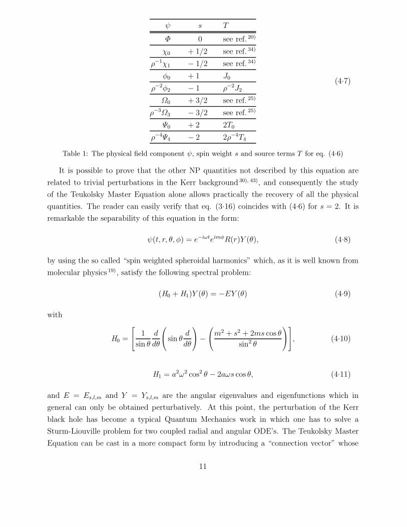
ψ s T

Φ 0 see ref. 20)

χ0 + 1/2 see ref. 34)

ρ−1χ1 − 1/2 see ref. 34)

φ0 + 1 J0

ρ−2φ2 − 1 ρ−2J2

Ω0 + 3/2 see ref. 25)

ρ−3Ω3 − 3/2 see ref. 25)

Ψ0 + 2 2T0

ρ−4Ψ4 − 2 2ρ−4T4

(4.7)

Table 1: The physical field component ψ, spin weight s and source terms T for eq. (4.6)

It is possible to prove that the other NP quantities not described by this equation are

related to trivial perturbations in the Kerr background 30), 43), and consequently the study

of the Teukolsky Master Equation alone allows practically the recovery of all the physical

quantities. The reader can easily verify that eq. (3.16) coincides with (4.6) for s = 2. It is

remarkable the separability of this equation in the form:

ψ(t, r, θ, φ) = e−iωteimφR(r)Y (θ), (4.8)

by using the so called “spin weighted spheroidal harmonics” which, as it is well known from

molecular physics 19), satisfy the following spectral problem:

(H0 + H1)Y (θ) = −EY (θ) (4.9)

with

H0 =

1

sin θ

d

dθ

sin θd

dθ

−m2 + s2 + 2ms cos θ

sin2 θ

, (4.10)

H1 = a2ω2 cos2 θ − 2aωs cos θ, (4.11)

and E = Es,l,m and Y = Ys,l,m are the angular eigenvalues and eigenfunctions which in

general can only be obtained perturbatively. At this point, the perturbation of the Kerr

black hole has become a typical Quantum Mechanics work in which one has to solve a

Sturm-Liouville problem for two coupled radial and angular ODE’s. The Teukolsky Master

Equation can be cast in a more compact form by introducing a “connection vector” whose

11

components are:

Γ t = − 1

Σ

[M(r2 − a2)

∆− (r + ia cos θ)

]

Γ r = − 1

Σ(r −M)

Γ θ = 0

Γ φ = − 1

Σ

[a(r −M)

∆+ i

cos θ

sin2 θ

]. (4.12)

It’s easy to prove that:

∇µΓµ = − 1

Σ, Γ µΓµ =

1

Σcot2 θ + 4ΨA

2 (4.13)

and consequently the Teukolsky Master Equation assumes the form:

[(∇µ + sΓ µ)(∇µ + sΓµ)− 4s2ΨA2 ]ψ(s) = 4πT (4.14)

where ΨA2 is the only non vanishing NP component of the Weyl tensor in the Kerr background

in the Kinnersley tetrad (4.4). Equation (4.14) gives a common structure for these massless

fields in the Kerr background variating the ”s” index. In fact, the first part in the lhs

represents (formally) a D’Alembertian, corrected by taking into account the spin-weight and

the second one is a curvature (Weyl) term linked to the “s” index too. This particular form

of the Teukolsky Master Equation forces us to extend this analysis in the next sections.

§5. Generalized wave equations

The compact form of Teukolsky Master Equation we have shown suggests a connec-

tion between the perturbation theory and a sort of generalized wave equations which differ

from the standard ones by curvature terms. In fact generalized wave operators are know

as De Rham-Lichnerowicz Laplacians and the curvature terms which make them different

from the ordinary ones are given by the Weitzenbock formulas. Mostly known examples in

electromagnetism are

• the wave equation for the vector potential Aµ21):

∇α∇αAµ − RµλAλ = −4πJµ , ∇αAα = 0 (5.1)

• the wave equation for the Maxwell tensor 24):

∇µ∇µFνλ +RρµνλFρµ − Rρ

λFνρ +RρνFλρ = −8π∇[µJν] (5.2)

12

while for the gravitational case one has

• the wave equation for the metric perturbations (gravitational waves) 21):

∇α∇αhµν + 2Rαβµν hαβ − 2Rα(µhν)

α = 0,

∇αhµα = 0, hµν = hµν −

1

2gµνhα

α (5.3)

• the wave equation for the Riemann Tensor 21) (in vacuum for simplicity)

∇µ∇µRαβγδ − RαβρσRγδρσ − 2(RαργσRβ

ρδσ −RαρδσRβ

ργ

σ) = 0 . (5.4)

These equations are “non minimal,” in the sense that they cannot be recovered by a minimal

substitution from their flat space counterparts. A similar situation holds in the standard

Quantum Field Theory for the electromagnetic Dirac equation. In fact, applying for instance

to the Dirac equation an “ad hoc” first order differential operator one gets the second order

Dirac equation 27), 28)

(i/∂ − e/A+m)(i/∂ − e/A−m)ψ =[(i∂µ − eAµ)(i∂µ − eAµ)− e

2σµνFµν −m2

]ψ = 0, (5.5)

where the notation is obvious. It is easy to recognize in eq. (5.5) a generalized Laplacian and

a curvature (Maxwell) term applied to the spinor. Moreover this equation is “non minimal”,

in the sense that the curvature (Maxwell) term cannot be recoverered by electromagnetic

minimal substitution in the standard Klein-Gordon equation for the spinor components.

The analogous second order Dirac equation in presence of a gravitational field also has a non

minimal curvature term 22), 23) and reduces to the form:

(∇α∇α +m2 +1

4R)ψ = 0 (5.6)

Quite recently it was shown by Mohanty and Prasanna 24), that the Maxwell tensor wave

equation (5.2) could be framed into the context of the QED vacuum polarization in a back-

ground gravitational field. They start from a classical work of Drummond and Hathrell 26)

which derives higher derivative coupling arising from the QED loop corrections to the

graviton-photon vertex, encoded in the Lagrangian, valid for ω2 < α/m2e (α is the fine

structure constant and me is the electron mass):

L = −1

4FµνF

µν + aRFµνFµν + bRµνF

µσF νσ + cRµνστF

µνF στ (5.7)

with the coefficients a = − 5720

απ, b = 26

720απ, c = − 2

720απ. The physics of these “tidal” terms

is that the effect of virtual electron loops gives to the photon a typical size proportional to

13

the Compton wavelenght of the electron λc. The field equations obtained from the modified

lagrangian (5.7) are:

∇µFµν +Ων = 0 (5.8)

where Ων represents the non linear quantum correction the explicit (long) form of which is

given in 24). Manipulating the previous relation one gets the wave equation:

∇µ∇µFνλ + RρµνλFρµ +Rρ

λFνρ − RρνFλρ+ [∇νΩλ −∇λΩν ] = 0 . (5.9)

In the range of validity of the effective action the Riemann and Ricci terms in the curl

brackets of (5.9) which are present in Einstein’s gravity are larger than the terms in the

square brackets, arising from the loop corrections, and consequently it is clear that the

classical second order wave equation for the Maxwell tensor describes with good accuracy

this quantum phenomenon too.

§6. Vacuum gravitational fields

The Weyl and the Riemann tensor are connected by the relation:

Rαβγδ = Cαβγδ +1

2(gαγRβδ − gβγRαδ − gαδRβγ + gβδRαγ)

−1

6(gαγgβδ − gαδgβγ)R , (6.1)

In a vacuum spacetime, Rαβ = 0, R = 0 and consequently the Riemann tensor coincides with

the Weyl one. The Weyl tensor in vacuum satisfies the generalized de Rham wave equation

(the vertical bar indicates the covariant derivative)

∆(dR)Ca1a2a3a4 = Ca1a2a3a4 |b|b + (Cbca1a2Cbca3a4 + 4Cb

a1

c[a4Ca3]cba2) = 0 .

(6.2)

The name “generalized de Rham wave equation” comes from the nice compact form which

can be given to this equation

∆(dR)Ca1a2a3a4 = (δD +Dδ)Ca1a2a3a4 = 0 , (6.3)

by using the divergence operator δ and the covariant exterior derivative D 39) - 41) (the diver-

gence operator δ and the covariant exterior derivative D must not be confused with the NP

frame derivatives denoted by the same symbols). This is the most natural generalization to

tensor-valued forms of the ordinary de Rham wave operator

∆(dR) = δd+ dδ, (6.4)

14

whose action is defined only on ordinary differential forms. A detailed study of the general-

ized de Rham operator will be discussed elsewhere 38).

The explicit form taken by [∆(dR)C]abcd = 0 in the Newman-Penrose formalism is now

derived and simplified somewhat using the commutator identities to eliminate some second

derivatives and the Bianchi and Ricci identities to eliminate some coupling terms between

different Weyl tensor scalars.

• [∆(dR)C]1313 = 0 (wave equation for Ψ0)

Recalling that Ψ0 = −C1313, select the 1313 component of eq. (6.2)

[−D∆−∆D + δ∗δ + δδ∗ + (9γ + γ∗ − µ− µ∗)D + (7ε− ε∗ + ρ∗ + ρ)∆

+ (β∗ + π − 9α− τ ∗)δ + (π∗ − τ − 7β − α∗)δ∗ + 4(Dγ +∆ε− δα− δ∗β)

+ 4(αα∗ − ρ∗γ + τ ∗β + τπ − β∗β − 8γε− εγ∗ + γε∗ − απ∗ + µε− βπ − σλ+ κν + τα + 8αβ − ρµ− ργ + µ∗ε + 3Ψ2)]Ψ0 + 4[2ρδ + 2σδ∗ − 2τD − 2κ∆

+ δρ−Dτ + δ∗σ −∆κ+ π∗ρ− ρα∗ + 5τε− τε∗ − 5ρβ + τρ∗ + σπ − κµ∗

− κµ− 7σα + κγ∗ + 7κγ − στ ∗ + σβ∗ − 3Ψ1]Ψ1 + [24(σρ− κτ)]Ψ2 = 0 .

(6.5)

This equation only contains second order directional derivatives of Ψ0, which can be rewritten

first using the identities

D∆+∆D = 2D∆+ [∆,D]

δδ∗ + δ∗δ = 2δδ∗ + [δ∗, δ] (6.6)

and then the commutators in these expressions can be replaced by first order derivatives

using the commutator identities (2.7)1 and (2.7)4, in order to reduce the number of second

order differential operators acting on Ψ0.

Equation (6.5) then becomes

[−2D∆+ 2δδ∗ + (8γ − 2µ)D + (6ε− 2ε∗ + 2ρ∗)∆ + (2π − 8α)δ

+ (2π∗ − 6β − 2α∗)δ∗ + 4(Dγ +∆ε− δα− δ∗β) + 4(αα∗ − ρ∗γ+ τ ∗β + τπ − β∗β − 8γε− εγ∗ + γε∗ − απ∗ + µε− βπ − σλ+ κν + τα + 8αβ − ρµ− ργ + µ∗ε + 3Ψ2)]Ψ0 + 4[2ρδ + 2σδ∗ − 2τD − 2κ∆

+ δρ−Dτ + δ∗σ −∆κ + π∗ρ− ρα∗ + 5τε− τε∗ − 5ρβ + τρ∗ + σπ − κµ∗

− κµ− 7σα + κγ∗ + 7κγ − στ ∗ + σβ∗ − 3Ψ1]Ψ1 + [24(σρ− κτ)]Ψ2 = 0

(6.7)

Next the Bianchi identities can be used to simplify this expression and introduce terms

involving Ψ0 to decouple it whenever possible. This task is achieved by the elimination of

15

two directional derivatives of Ψ1 in eq. (6.7) using two Bianchi identities

R13[13|4] = 0 : DΨ1 − δ∗Ψ0 + (4α− π)Ψ0 − 2(2ρ+ ε)Ψ1 + 3κΨ2 = 0 ,

R13[13|2] = 0 : δΨ1 −∆Ψ0 + (4γ − µ)Ψ0 − 2(2τ + β)Ψ1 + 3σΨ2 = 0 . (6.8)

Equation (6.7) then becomes

[−2D∆ + 2δδ∗ + 2(4γ − µ)D + 2(3ε− ε∗ + ρ∗ + 4ρ)∆ + 2(π − 4α)δ

+ 2(π∗ − 3β − α∗ − 4τ)δ∗ + 4(Dγ +∆ε− δα− δ∗β) + 4(αα∗ − ρ∗γ+ τ ∗β − τπ − β∗β − 8γε− εγ∗ + γε∗ − απ∗ + µε− βπ − σλ+ κν + 9τα + 8αβ + ρµ− 9ργ + µ∗ε + 3Ψ2)]Ψ0 + 4[2σδ∗ − 2κ∆

+ δρ−Dτ + δ∗σ −∆κ+ π∗ρ− ρα∗ + τε− τε∗ − ρβ + τρ∗ + σπ − κµ∗

− κµ− 7σα + κγ∗ + 7κγ − στ ∗ + σβ∗ − 3Ψ1]Ψ1 = 0 .

(6.9)

Finally this (exact) equation can be given a Teukolsky-like form which is very helpful in

type D geometries where most of the known results have been derived. To accomplish this

additional step, multiply the equation by −1/2 and use three Ricci identities in two different

ways: a) in (6.9) first use the identities

[1/2(R1212 − R3412)] : ∆ε = Dγ − α(τ + π∗)− β(τ ∗ + π)+

+ γ(ε + ε∗) + ε(γ + γ∗)− τπ + νκ− Ψ2 ,

[1/2(R1234 − R3434)] : δ∗β = δα− (µρ− λσ)− αα∗ − ββ∗++ 2αβ − γ(ρ− ρ∗)− ε(µ − µ∗) + Ψ2 ;

(6.10)

b) rewrite the other Ricci identity [R2431] in the following form

[R2431] : Dµ− δπ − (ρ∗µ+ σλ)− π(π∗ − α∗ + β) + µ(ε+ ε∗) + νκ− Ψ2 = 0 , (6.11)

multiply it by Ψ0 and c) add this (which is actually zero) to the wave equation. The result

is

[(D − 3ε+ ε∗ − 4ρ− ρ∗)(∆+ µ− 4γ)− (δ + π∗ − α∗ − 3β − 4τ)

(δ∗ + π − 4α)− 3Ψ2]Ψ0 + 3(σλ− κν)Ψ0 + 2[2κ∆− 2σδ∗ − δ∗σ +∆κ

− δρ+Dτ − 7κγ − β∗σ + 7σα + τ ∗σ + κµ∗ + κµ− ρπ∗ + τε∗ + βρ

− ετ − κγ∗ − πσ − τρ∗ + ρα∗ + 3Ψ1]Ψ1 = 0 ;

(6.12)

d) finally use in eq. (6.12) two other Ricci identities

[R3143] : δρ− δ∗σ = ρ(α∗ + β)− σ(3α− β∗) + τ(ρ− ρ∗) + κ(µ− µ∗)− Ψ1 ,

[R1312] : Dτ −∆κ = ρ(τ + π∗) + σ(τ ∗ + π) + τ(ε− ε∗)− κ(3γ + γ∗) + Ψ1. (6.13)

16

The final form for eq. (6.12) is then

[(D − 3ε+ ε∗ − 4ρ− ρ∗)(∆+ µ− 4γ)− (δ + π∗ − α∗ − 3β − 4τ)

(δ∗ + π − 4α)− 3Ψ2]Ψ0 + 3(σλ− κν)Ψ0 + [4κ∆− 4σδ∗ − 4δ∗σ + 4∆κ

− 20κγ − 4β∗σ + 20σα+ 4τ ∗σ + 4κµ∗ − 4κγ∗ + 10Ψ1]Ψ1 = 0 ,

(6.14)

which is the exact form for the same equation for Ψ0 found by Teukolsky in the very special

case of a type D geometry in the first order perturbation regime (see below). Moreover

this equation coincides with that obtained by Stewart and Walker 10) following a different

approach and in the Geroch-Held-Penrose (GHP) formalism 33)

( IP′IP− ∂′ ∂ − ρ′IP− 5ρIP

′ + τ ∂ + 5τ ∂ ′ + 4σσ′ − 4κκ′ − 10Ψ2)Ψ0

+ [4IP′κ− 4 ∂′σ − 4(ρ′ − 2ρ′)κ+ 4(τ − 2τ ′)σ + 10Ψ1]Ψ1

+ (−4σIP + 4κ ∂ − 12κτ + 12ρσ)Ψ2 = 0 .

(6.15)

The equivalence of (6.14) and (6.15) is now explicitly shown. Recall the action of the

two-index p, q-operators IP, IP′, ∂, ∂′ on two-index p, q-objects. Taking into account the

weights of the Ψn’s (i.e., p, q = 4−2n, 0), those of the spin coefficients and the definition

of the weighted derivative operator of an object η (which increases its p, q indices)

IPη = (D − pε− qε∗)η, increasing of type +1,+1,IP′η = (∆− pγ − qγ∗)η, increasing of type −1,−1, ∂η = (δ − pβ − qα∗)η, increasing of type +1,−1, ∂′η = (δ∗ − pα− qβ∗)η, increasing of type −1,+1,

(6.16)

eq. (6.15) becomes:

[(∆− 5γ − γ∗)(D − 4ε)− (δ∗ − 5α+ β∗)(δ − 4β) + µ∗(D − 4ε)

− 5ρ(∆− 4γ) + τ ∗(δ − 4β) + 5τ(δ∗ − 4α)− 4(σλ− κν)− 10Ψ2]Ψ0

+ (−4σD + 4κδ − 12κτ + 12ρσ)Ψ2 + [4(∆− 3γ − γ∗)κ− 4(δ∗ − 3α+ β∗)σ − 4(−µ∗ + 2µ)κ+ 4(τ ∗ + 2π)σ + 10Ψ1)]Ψ1 = 0 ,

(6.17)

where the second order operator has to be rewritten via the commutation rules (2.7).

Then, by using the two Ricci identities 1/2[R1212 − R3412] and 1/2[R1234 − R3434] (see

eq. (6.10)), adding equation [R2431] multiplied by Ψ0 and using the two Bianchi identities

R13[43|2] = 0 and R13[21|4] = 0, namely:

∆Ψ1 − δΨ2 − νΨ0 − 2(γ − µ)Ψ1 + 3τΨ2 − 2σΨ3 = 0 , R13[43|2] = 0 ,

δ∗Ψ1 −DΨ2 − λΨ0 + 2(π − α)Ψ1 + 3ρΨ2 − 2κΨ3 = 0 , R13[21|4] = 0 ,(6.18)

17

one gets exactly eq. (6.14).

• [∆(dR)C]2424 = 0 (wave equation for Ψ4)

The equation for Ψ4 can be immediately obtained from the equation for Ψ0 using the ex-

change symmetry l↔ n, m↔ m∗ of the Newman-Penrose quantities. Under this operation,

eq. (6.14) becomes:

[(∆ + 3γ − γ∗ + 4µ+ µ∗)(D + 4ε− ρ)− (δ∗ − τ ∗ + β∗ + 3α + 4π)

(δ − τ + 4β)− 3Ψ2]Ψ4 + 3(σλ− κν)Ψ4 + [4λδ − 4νD + 4δλ− 4Dν

− 20νε− 4α∗λ+ 20λβ + 4π∗λ+ 4νρ∗ − 4νε∗ + 10Ψ3]Ψ3 = 0 .

(6.19)

Working in the GHP formalism, the corresponding relation found by Stewart and Walker10) is:

[( IP′IP− ∂′ ∂ − (4ρ′ + ρ′)IP− ρIP

′ + (4τ ′ + τ) ∂ + τ ∂ ′ + 4ρρ′ − 4ττ ′ − 2Ψ2]Ψ4

+ [4IPκ′ − 4 ∂σ′ − 4(ρ− 2ρ)κ′ + 4(τ − 2τ)σ′ + 10Ψ3]Ψ3

+ [−4σ′IP′ + 4κ′ ∂′ − 12κ′τ ′ + 12ρ′σ′]Ψ2 = 0.

(6.20)

• [∆(dR)C]1213 = 0 (wave equation for Ψ1)

Selecting the component C1213 (Ψ1 = −C1213) in eq. (6.2) one has

[δδ∗ + δ∗δ −D∆−∆D + (γ∗ + 5γ − µ− µ∗)D + (ρ + ρ∗ + 3ε− ε∗)∆+ (π + β∗ − τ ∗ − 5α)δ + (π∗ − 3β − τ − α∗)δ∗ + 2(Dγ +∆ε− δα− δ∗β+ 5τπ + αα∗ − 4γε− ργ − ρ∗γ + µ∗ε− εγ∗ − ββ∗ + γε∗ − βπ− 5σλ+ βτ∗ − απ∗ + µε+ 4αβ − 5ρµ+ τα + 5κν − 3Ψ2)]Ψ1

+ [2νD + 2π∆− 2λδ − 2µδ∗ +Dν +∆π − δλ− δ∗µ+ τ ∗µ− νρ∗ + τλ

+ πµ∗ + λα∗ − 7γπ − 5νε + 7αµ− πγ∗ + νε∗ − νρ + 5λβ − λπ∗ − µβ∗ + 6Ψ3]Ψ0

+ 3[−2τD − 2κ∆+ 2ρδ + 2σδ∗ −Dτ −∆κ + δρ+ δ∗σ + β∗σ − βρ− στ ∗

− κµ∗ + κγ∗ − 3σα− τε∗ + ετ − α∗ρ+ τρ∗ + 3γκ− µκ+ σπ + ρπ∗]Ψ2

+ 12(σρ− κτ)Ψ3 = 0 .

(6.21)

Using the commutation rules (2.7), multiplying by −1/2, and using the six Bianchi

identities R13[13|4] = 0, R13[13|2] = 0, R13[21|4] = 0, R13[43|2] = 0, R42[13|2] = 0 R42[13|4] = 0

and the five Ricci identities [R3143], [R1312], [R2443], [R2421], [12(R1234 − R3434))], eq. (6.21)

becomes:

18

[D∆− δδ∗ + 2(µ− γ)D + (−3ρ− ρ∗ − ε + ε∗)∆+ 2(α− π)δ + (β + α∗ + 3τ − π∗)δ∗

−Dγ −∆ε + 2δα + 2ρ∗γ − γε∗ + απ∗ + κν + εγ∗ + 6ργ + 4γε− 6ρµ− 7τα + 5τπ − βτ ∗

− 2αα∗ − 2αβ + 3βπ − 4µε+ 7Ψ2]Ψ1 + [λδ − νD + δλ−Dν − 3τλ+ νε− α∗λ+ 3ρν − νε∗ + λπ∗ + νρ∗ − βλ− 2Ψ3]Ψ0 + 3[κδ − σD + 2σρ+ 2κβ − 2κτ − 2σε]Ψ3

+ 3[∆κ− δ∗σ − 2µκ+ 2σπ − σβ∗ + κµ∗ − 3κγ + στ ∗ − κγ∗ + 3ασ]Ψ2 = 0.

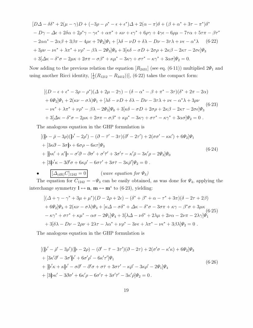
(6.22)

Now adding to the previous relation the equation [R2431] (see eq. (6.11)) multiplied 2Ψ1 and

using another Ricci identity, [12(R1212 − R3412))], (6.22) takes the compact form:

[(D − ε+ ε∗ − 3ρ− ρ∗)(∆ + 2µ− 2γ)− (δ − α∗ − β + π∗ − 3τ)(δ∗ + 2π − 2α)

+ 6Ψ2]Ψ1 + 2(κν − σλ)Ψ1 + [λδ − νD + δλ−Dν − 3τλ+ νε− α∗λ+ 3ρν

− νε∗ + λπ∗ + νρ∗ − βλ− 2Ψ3]Ψ0 + 3[κδ − σD + 2σρ+ 2κβ − 2κτ − 2σε]Ψ3

+ 3[∆κ− δ∗σ − 2µκ+ 2σπ − σβ∗ + κµ∗ − 3κγ + στ ∗ − κγ∗ + 3ασ]Ψ2 = 0 .

(6.23)

The analogous equation in the GHP formulation is

[(IP− ρ− 3ρ)(IP′ − 2ρ′)− ( ∂ − τ ′ − 3τ)( ∂′ − 2τ ′) + 2(σσ′ − κκ′) + 6Ψ2]Ψ1

+ [3κ ∂ − 3σIP + 6σρ− 6κτ ]Ψ3

+ [IPκ′ + κ′IP− σ′ ∂ − ∂σ′ + σ′τ ′ + 3σ′τ − κ′ρ− 3κ′ρ− 2Ψ3]Ψ0

+ [3IP′κ− 3 ∂′σ + 6κρ′ − 6στ ′ + 3στ − 3κρ′]Ψ2 = 0 .

(6.24)

• [∆(dR)C]1242 = 0 (wave equation for Ψ3)

The equation for C1242 = −Ψ3 can be easily obtained, as was done for Ψ4, applying the

interchange symmetry l↔ n, m↔m∗ to (6.23), yielding:

[(∆+ γ − γ∗ + 3µ+ µ∗)(D − 2ρ+ 2ε)− (δ∗ + β∗ + α− τ ∗ + 3π)(δ − 2τ + 2β)

+ 6Ψ2]Ψ3 + 2(κν − σλ)Ψ3 + [κ∆− σδ∗ +∆κ− δ∗σ − 3σπ + κγ − β∗σ + 3µκ

− κγ∗ + στ ∗ + κµ∗ − ασ − 2Ψ1]Ψ4 + 3[λ∆− νδ∗ + 2λµ+ 2να− 2νπ − 2λγ]Ψ1

+ 3[δλ−Dν − 2ρν + 2λτ − λα∗ + νρ∗ − 3νε + λπ∗ − νε∗ + 3βλ]Ψ2 = 0 .

(6.25)

The analogous equation in the GHP formulation is

[(IP′ − ρ′ − 3ρ′)(IP− 2ρ)− ( ∂′ − τ − 3τ ′)( ∂ − 2τ) + 2(σ′σ − κ′κ) + 6Ψ2]Ψ3

+ [3κ′ ∂′ − 3σ′IP′ + 6σ′ρ′ − 6κ′τ ′]Ψ1

+ [IP′κ+ κIP

′ − σ ∂′ − ∂′σ + στ + 3στ ′ − κρ′ − 3κρ′ − 2Ψ1]Ψ4

+ [3IPκ′ − 3 ∂σ′ + 6κ′ρ− 6σ′τ + 3σ′τ ′ − 3κ′ρ]Ψ2 = 0 .

(6.26)

19

• [∆(dR)C]1342 = 0 (wave equation for Ψ2)

Selecting the component 1342 of (6.2) (Ψ2 = −C1342) one has

[−D∆−∆D + δδ∗ + δ∗δ + (γ + γ∗ − µ− µ∗)D + (ρ+ ρ∗ − ε− ε∗)∆+ (π + β∗ − α− τ ∗)δ + (π∗ + β − α∗ − τ)δ∗ + 12τπ − 12ρµ+ 12νκ− 12λσ − 6Ψ2]Ψ2

+ [4νD + 4π∆− 4λδ − 4µδ∗ + 2Dν + 2∆π − 2δλ− 2δ∗µ+ 2µτ ∗ − 6γπ + 2νε∗ − 2ρ∗ν

− 2µβ∗ + 2λβ + 2λα∗ + 2πµ∗ − 2πγ∗ − 2νε + 2τλ− 2ρν − 2λπ∗ + 6αµ+ 4Ψ3]Ψ1

+ [−4τD − 4κ∆+ 4ρδ + 4σδ∗ − 2Dτ − 2∆κ + 2δρ+ 2δ∗σ + 2π∗ρ− 2ε∗τ + 2τρ∗

− 2µκ+ 2ασ + 6ρβ − 2τ ∗σ + 2σβ∗ + 2πσ − 2κµ∗ − 2κγ − 6ετ − 2ρα∗ + 2κγ∗]Ψ3

+ [4ρσ − 4τκ]Ψ4 + [4λµ− 4νπ + 2Ψ4]Ψ0 = 0 .

(6.27)

Using the commutation rules (2.7), multiplying (6.27) by−1/2, and using the four Bianchi

identities R13[21|4] = 0, R13[43|2] = 0, R42[13|2] = 0 R42[13|4] = 0, the four Ricci identities [R3143],

[R1312], [R2443], [R2421] and adding eq. (6.11) once multiplied by 3Ψ2, relation (6.27) takes

the form:

[(D + ε+ ε∗ − 2ρ− ρ∗)(∆+ 3µ)− (δ + π∗ − 2τ + β − α∗)(δ∗ + 3π)]Ψ2

+ (3λσ − 3νκ)Ψ2 + 2[−νD + λδ −Dν + δλ+ νρ∗ + λπ∗ − 2τλ

− λα∗ + λβ − νε∗ − νε + 2ρν + Ψ3]Ψ1 + 2[κ∆− σδ∗ +∆κ

− δ∗σ + ασ + κµ∗ + 2µκ+ τ ∗σ − κγ∗ − γκ− 2πσ − σβ∗]Ψ3 − Ψ0Ψ4 = 0

(6.28)

The corresponding equation in the GHP formalism is

[(IP− 2ρ− ρ)(IP′ − 3ρ′)− ( ∂ − 2τ − τ ′)( ∂′ − 3τ ′) + 3(κκ′ − σσ′)]Ψ2

+2[κ′IP + IPκ′ − σ′ ∂ − ∂σ′ + 2τσ′ + σ′τ ′ − 2ρκ′ − κ′ρ]Ψ1

+2[κIP′ + IP

′κ− ∂′σ − σ ∂′ + Ψ1 + 2τ ′σ − 2ρ′κ+ τ σ − κρ′]Ψ3 − Ψ0Ψ4 = 0 .

(6.29)

At this point the complete set of (exact) wave equations satisfied by the Weyl scalars has

been given. We can now perform their perturbation expansion.

6.1. The perturbation theory

Introducing the operators:

T0 = [(D − 3ε + ε∗ − 4ρ− ρ∗)(∆+ µ− 4γ)− (δ + π∗ − α∗ − 3β − 4τ)(δ∗ + π − 4α)− 3Ψ2],

W0 = 3(σλ− κν),

P1 = [4κ∆− 4σδ∗ − 4δ∗σ + 4∆κ− 20κγ − 4β∗σ + 20σα+ 4τ ∗σ + 4κµ∗ − 4κγ∗ + 10Ψ1],

(6.30)

20

where the letter T0 here stands for the operator on Ψ0 found by Teukolsky in the perturbation

regime; this is a notation extending that due to Lousto and Campanelli 35). In the same way

a generic operator χ acting on Ψi will be denoted by χi. Thus, eq. (6.14) can be written as:

(T0 + W0)Ψ0 + P1Ψ1 = 0 . (6.31)

Performing the standard perturbation expansion of the various quantities a la Teukolsky:

Ψ0 = Ψ(0)0 + Ψ

(1)0 + Ψ

(2)0 + ..., σ = σ(0) + σ(1) + ...,D = D(0) +D(1) + ... and so on, one finds

[(T (0)0 + T (1)

0 + T (2)0 + ...) + (W(0)

0 + W(1)0 + W(2) + ...)](Ψ

(0)0 + Ψ

(1)0 + Ψ

(2)0 + ...)

+ (P(0)1 + P(1)

1 + P(2)1 + ...)(Ψ

(0)1 + Ψ

(1)1 + Ψ

(2)1 + ...) = 0 ,

(6.32)

giving an inductive procedure for obtaining a hierarchy of equations of the following type:

(T (0)0 + W(0)

0 )Ψ(0)0 + P(0)

1 Ψ(0)1 = 0,

(T (1)0 + W(1)

0 )Ψ(0)0 + (T (0)

0 + W(0)0 )Ψ

(1)0 + (P(0)

1 Ψ(1)1 + P(1)

1 Ψ(0)1 ) = 0,

...

(T (n)0 + W(n)

0 )Ψ(0)0 + (T (0)

0 + W(0)0 )Ψ

(n)0 + (P(n)

1 Ψ(0)1 + P(0)

1 Ψ(n)1 ) = S(n)

0 ,

(6.33)

where

S(n)0 = −

n−1∑p=1

[(T (n−p)0 + W(n−p)

0 )Ψ(p)0 + P(n−p)

1 Ψ(p)1 ] , (n ≥ 2) . (6.34)

For every n ≥ 2 perturbation equation, the “source term” S(n)0 is composed of quantities at

most of order (n− 1), which in principle are known.

For a type D background geometry it is well known that

κ(0) = σ(0) = λ(0) = ν(0) = 0,

Ψ(0)0 = Ψ

(0)1 = Ψ

(0)3 = Ψ

(0)4 = 0,

(6.35)

so W(0)0 = W(1)

0 = P(0)1 = 0 and the recurrence scheme (6.33) becomes:

0 = 0,

T (0)0 Ψ

(1)0 = 0,

...

T (0)0 Ψ

(n)0 = S(n)

0 .

(6.36)

21

One can study the perturbation of eq. (6.19) exactly in the same way as before. In fact,

defining the operators

T4 = [(∆+ 3γ − γ∗ + 4µ+ µ∗)(D + 4ε− ρ)− (δ∗ − τ ∗ + β∗ + 3α + 4π)

(δ − τ + 4β)− 3Ψ2],

P3 = [4λδ − 4νD + 4δλ− 4Dν − 20νε− 4α∗λ+ 20λβ + 4π∗λ+ 4νρ∗ − 4νε∗ + 10Ψ3],

W4 = 3(σλ− κν),

(6.37)

(where the letter T4 here stands for the operator on Ψ4 found by Teukolsky), eq. (6.19) can

be written as

(T4 + W4)Ψ4 + P3Ψ3 = 0 . (6.38)

The hierarchy of equations in this case is:

(T (0)4 + W(0)

4 )Ψ(0)4 + P(0)

3 Ψ(0)3 = 0,

(T (1)4 + W(1)

4 )Ψ(0)4 + (T (0)

4 + W(0)4 )Ψ

(1)4 + (P(0)

3 Ψ(1)3 + P(1)

3 Ψ(0)3 ) = 0,

...

(T (n)4 + W(n)

4 )Ψ(0)4 + (T (0)

4 + W(0)4 )Ψ

(n)4 + (P(n)

3 Ψ(0)3 + P(0)

3 Ψ(n)3 ) = S(n)

4 ,

(6.39)

where

S(n)4 = −

n−1∑p=1

[(T (n−p)4 + W(n−p)

4 )Ψ(p)4 + P(n−p)

3 Ψ(p)3 ], (n ≥ 2) . (6.40)

In the case of a type D geometry W(0)4 = W(1)

4 = P(0)3 = 0 and the set of equations (6.39)

becomes:

0 = 0,

T (0)4 Ψ

(1)4 = 0,

...

T (0)4 Ψ

(n)4 = S(n)

4 .

(6.41)

The previous results are an alternative but equivalent formulation of the work of Lousto and

Campanelli concerning the higher order perturbations of a type D vacuum metric. The same

perturbation formulation can easily be written for eqs. (6.23), (6.25) and (6.28) allowing a

systematic formulation of the gravitational perturbation for every vacuum spacetime. In

22

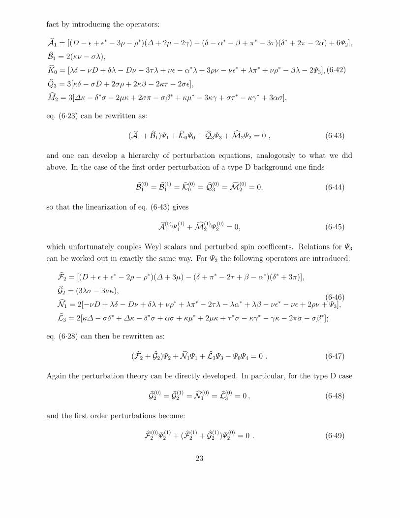
fact by introducing the operators:

A1 = [(D − ε + ε∗ − 3ρ− ρ∗)(∆+ 2µ− 2γ)− (δ − α∗ − β + π∗ − 3τ)(δ∗ + 2π − 2α) + 6Ψ2],

B1 = 2(κν − σλ),

K0 = [λδ − νD + δλ−Dν − 3τλ+ νε− α∗λ+ 3ρν − νε∗ + λπ∗ + νρ∗ − βλ− 2Ψ3],

Q3 = 3[κδ − σD + 2σρ+ 2κβ − 2κτ − 2σε],

M2 = 3[∆κ− δ∗σ − 2µκ+ 2σπ − σβ∗ + κµ∗ − 3κγ + στ ∗ − κγ∗ + 3ασ],

(6.42)

eq. (6.23) can be rewritten as:

(A1 + B1)Ψ1 + K0Ψ0 + Q3Ψ3 + M2Ψ2 = 0 , (6.43)

and one can develop a hierarchy of perturbation equations, analogously to what we did

above. In the case of the first order perturbation of a type D background one finds

B(0)1 = B(1)

1 = K(0)0 = Q(0)

3 = M(0)2 = 0, (6.44)

so that the linearization of eq. (6.43) gives

A(0)1 Ψ

(1)1 + M(1)

2 Ψ(0)2 = 0, (6.45)

which unfortunately couples Weyl scalars and perturbed spin coefficents. Relations for Ψ3

can be worked out in exactly the same way. For Ψ2 the following operators are introduced:

F2 = [(D + ε + ε∗ − 2ρ− ρ∗)(∆+ 3µ)− (δ + π∗ − 2τ + β − α∗)(δ∗ + 3π)],

G2 = (3λσ − 3νκ),

N1 = 2[−νD + λδ −Dν + δλ+ νρ∗ + λπ∗ − 2τλ− λα∗ + λβ − νε∗ − νε + 2ρν + Ψ3],

L3 = 2[κ∆− σδ∗ +∆κ− δ∗σ + ασ + κµ∗ + 2µκ+ τ ∗σ − κγ∗ − γκ− 2πσ − σβ∗];

(6.46)

eq. (6.28) can then be rewritten as:

(F2 + G2)Ψ2 + N1Ψ1 + L3Ψ3 − Ψ0Ψ4 = 0 . (6.47)

Again the perturbation theory can be directly developed. In particular, for the type D case

G(0)2 = G(1)

2 = N (0)1 = L(0)

3 = 0 , (6.48)

and the first order perturbations become:

F (0)2 Ψ

(1)2 + (F (1)

2 + G(1)2 )Ψ

(0)2 = 0 . (6.49)

23

Thus, even in the very special case of a type D geometry, the perturbation equations for

Ψ1,Ψ2 and Ψ3 are coupled—order by order—with other perturbation quantities. This is due

to the presence, in the exact equations, of terms involving Ψ2 which are responsible for the

appearance of the perturbations of the spin coefficents and of the directional derivatives.

To obtain decoupled equations for these three Weyl scalars in the perturbation regime, in

principle, one has to define linear operators with derivatives of order higher than the second.

We conclude this section by pointing out that our perturbation relations (6.36) and (6.41)

assume a more compact form if compared with those found by Lousto and Campanelli be-

cause of the completely different approach and the number of simplifying operations (always

explicitly specified) that we perform at the level of the exact theory. They use ‘background

operators’ acting on the exact Bianchi identities and then linearize the results order by order

(see also their remark after eq. (6) in 35)), following the Teukolsky prescription. The way of

using exact ‘ad hoc’ operators acting on the exact Bianchi identities and then linearizing the

results was introduced by Stewart and Walker but only for first order perturbations.

By extending such a prescription to any order one obtains our relations. The de Rham

Laplacian mediates this task at the level of the exact theory, also explaining the nature (i.e.

exact ‘wave equations in curved spacetime’ for some of the NP Weyl and Maxwell scalars)

of the relations found algebraically by Stewart and Walker.

§7. Vacuum spacetimes: test electromagnetic fields

In this section we study the electromagnetic field equation in the absence of sources,

Jµ = 0. This choice has to be related to the “exact” (in the sense of the field equations)

nature of our approach, which goes beyond the perturbation level and would be corrupted

by the introduction of a source term without the automatic appearance of a corresponding

term in the Riemann tensor. On the other hand, eq. (7.1) below is itself an approximation,

because the exact field equations should include the Riemann and Ricci terms created by the

EM field and should be coupled to the gravitational de Rham Laplacian. The formulation

presented here is based on the hypothesis of test fields (no backreaction) and the goal of

this analysis is to recover the existing perturbation theory, including the work of Teukolsky,

Fackerell and Ipser and many other authors.

The sourcefree Maxwell equations δF = 0 = dF for the Maxwell 2-form F (representable

as 4 complex equations for the associated NP scalars φ0, φ1, φ2, namely eqs. (330)–(333) of

Chapter 1 of 37)) immediately imply the vanishing of the de Rham Laplacian of the Maxwell

2-form. In a vacuum spacetime, this takes the form

[∆(dR)F ]ab = Fab|c|c + CabcdFcd = 0 , (7.1)

24

Expressing these equations in the Newman-Penrose formalism, one has the following wave

equations.

• [∆(dR)F ]13 = 0 (wave equation for φ0)

Studying the component“13” of (7.1) we get the equation for φ0:

[D∆+∆D − δ∗δ − δδ∗ + (−5γ − γ∗ + µ+ µ∗)D + (−3ε + ε∗ − ρ∗ − ρ)∆

+ (−β∗ − π + 5α+ τ ∗)δ + (−π∗ + τ + 3β + α∗)δ∗ + 2(δ∗β + δα−Dγ −∆ε+ γ∗ε− γε∗ − τπ + γρ∗ + π∗α + 4γε− βτ ∗ + ρµ+ ββ∗ − εµ∗ − αα∗ − 4αβ

+ ργ − κν + βπ + σλ− τα− µε− Ψ2]φ0 + [4(τD + κ∆− ρδ − σδ∗)+ 2(Dτ +∆κ− δρ− δ∗σ + ε∗τ − ρπ∗ − ετ + στ ∗ − κγ∗ − τρ∗ − σβ∗ + ρα∗

+ µκ+ µ∗κ + βρ− σπ − 3κγ + 3ασ + 2Ψ1)]φ1 + [4κτ − 4σρ− 2Ψ0]φ2 = 0 .

(7.2)

First we use the commutation rules (2.7); the next step is to divide the resulting equation

by 2 and to use the two Maxwell equations:

(D − 2ρ)φ1 − (δ∗ + π − 2α)φ0 + κφ2 = 0, (7.3)

(δ − 2τ)φ1 − (∆ + µ− 2γ)φ0 + σφ2 = 0, (7.4)

to eliminate two of the directional derivatives of φ1. Then using four Ricci identities:

[1/2(R1212 − R3412)] : ∆ε = Dγ − α(τ + π∗)− β(τ ∗ + π) + γ(ε + ε∗)

+ ε(γ + γ∗)− τπ + νκ− Ψ2,

[1/2(R1234 − R3434)] : δ∗β = δα− (µρ− λσ)− αα∗ − ββ∗ + 2αβ

− γ(ρ− ρ∗)− ε(µ− µ∗) + Ψ2,

(7.5)

together with the two in (6.13), rewriting the Ricci identity [R2431] as in (6.11), multiplying

it by φ0 and adding the resulting quantity (which is actually zero) to the wave equation one

obtains:

[(D − ε + ε∗ − 2ρ− ρ∗)(∆+ µ− 2γ)− (δ − β − α∗ − 2τ + π∗)(δ∗ + π − 2α)]φ0

+ (σλ− κν)φ0 + 2[κ∆− σδ∗ +∆κ− δ∗σ − κγ∗ − σβ∗ + κµ∗ + στ ∗ + 3ασ

− 3κγ + 2Ψ1]φ1 − Ψ0φ2 = 0 ,

(7.6)

where in the first line it is easy to recognize the operator found by Teukolsky for the elec-

tromagnetic perturbations of a type D metric. One can also verify that (7.6) is the electro-

magnetic equation of Stewart and Walker in the GHP formalism:

[IPIP′ − ∂ ∂′ − ρ′IP− (2ρ+ ρ)IP

′ + τ ′ ∂ + (2τ + τ ′) ∂′ + 2ρρ′ − 2ττ ′ + Ψ2]φ0

+ [2IP′κ− 2 ∂′σ − 2κ(ρ′ − 2ρ′) + 2σ(τ − 2τ ′) + 4Ψ1]φ1 + [2κ ∂ − 2σIP

+ 2ρσ − 2κτ − Ψ0]φ2 = 0 .

(7.7)

25

In fact “translating” (7.7) into the standard Newman-Penrose form one gets:

[(D − ε+ ε∗)(∆− 2γ)− (δ − β − α∗)(δ∗ − 2α) + µ(D − 2ε)

− (2ρ+ ρ∗)(∆− 2γ)− π(δ − 2β) + (2τ − π∗)(δ∗ − 2α)− 2ρµ+ 2τπ + Ψ2]φ0

+ 2[(∆− 3γ − γ∗)κ− (δ∗ − 3α + β∗)σ + κ(µ∗ − 2µ) + σ(τ ∗ + 2π) + 2Ψ1]φ1

+ [2κ(δ + 2β)− 2σ(D + 2ε) + 2ρσ − 2κτ − Ψ0]φ2 = 0 .

(7.8)

Using the following two Maxwell equations:

(D − ρ + 2ε)φ2 − (δ∗ + 2π)φ1 + λφ0 = 0,

(δ − τ + 2β)φ2 − (∆+ 2µ)φ1 + νφ0 = 0,(7.9)

in the previous equation and adding the Ricci identity [R2431] (see eq. 6.11) multiplied by

φ0, one finds identically eq. (7.6).

• [∆(dR)F ]24 = 0 (wave equation for φ2)

The equation for φ2 can be immediately obtained form eq. (7.6). Using the exchange

symmetry l ↔ n, m ↔ m∗ of the Newman-Penrose quantities and the relation (2.18), one

gets

− [(∆ + γ − γ∗ + 2µ+ µ∗)(D − ρ + 2ε)− (δ∗ + α + β∗ + 2π − τ ∗)(δ − τ + 2β)]φ2

+ (σλ− κν)φ2 + 2[λδ − νD + δλ−Dν − νε∗ − λα∗ + νρ∗ + λπ∗ + 3βλ

− 3νε + 2Ψ3]φ1 − Ψ4φ0 = 0 .

(7.10)

The overall minus factor in our case can be eliminated but this form is convenient for further

developments in the presence of sources. The GHP analogue of this equation is

[IP′IP− ∂′ ∂ − ρIP

′ − (2ρ′ + ρ′)IP + τ ∂ ′ + (2τ ′ + τ) ∂ + 2ρ′ρ− 2τ ′τ + Ψ2]φ2

+ [2IPκ′ − 2 ∂σ′ − 2κ′(ρ− 2ρ) + 2σ′(τ ′ − 2τ) + 4Ψ3]φ1 + [2κ′ ∂′ − 2σ′IP

′

+ 2ρ′σ′ − 2κ′τ ′ − Ψ4]φ0 = 0.

(7.11)

• [∆(dR)F ]12 − [∆(dR)F ]34 = 0 (wave equation for φ1)

To obtain the equation for φ1 one has to subtract the components “12” and “34” of (7.1)

in order to eliminate all the φ∗n terms. The resulting wave equation, divided by a factor of

26

2, is:

[D∆+∆D − δ∗δ − δδ∗ + (−γ − γ∗ + µ+ µ∗)D + (ε + ε∗ − ρ∗ − ρ)∆

+ (−β∗ − π + α + τ ∗)δ + (−π∗ + τ − β + α∗)δ∗ + 4(ρµ+ λσ − τπ − νκ + Ψ2)]φ1

[−2νD − 2π∆+ 2λδ + 2µδ∗ −Dν −∆π + δλ+ δ∗µ− λα∗ + ρν + πγ∗ − µτ ∗

− τλ− 3αµ+ λπ∗ − πµ∗ + µβ∗ − λβ − νε∗ + νρ∗ + 3γπ + νε− 2Ψ3]φ0

+ [2τD + 2κ∆− 2ρδ − 2σδ∗ +Dτ +∆κ− δρ− δ∗σ − σπ − τρ∗ + γκ− κγ∗

+ 3τε + τ ∗σ − 3ρβ + µ∗κ− ασ + τε∗ − σβ∗ + ρα∗ + µκ− ρπ∗ − 2Ψ1]φ2 = 0.

(7.12)

The procedure to simplify the previous relations is the usual one. The starting point is

to rewrite the second order part by using (6.6); dividing the resulting equation by 2 and

using all four NP Maxwell equations, some of the directional derivatives of φ0 and φ2 are

eliminated in favor of the derivatives of φ1. Now, using the Ricci identies: (6.10), (6.13) and

[R2443] : δλ− δ∗µ = ν(ρ− ρ∗) + π(µ− µ∗) + µ(α + β∗) + λ(α∗ − 3β)− Ψ3 ,

[R2421] : Dν −∆π = µ(π + τ ∗) + λ(π∗ + τ) + π(γ − γ∗)− ν(3ε + ε∗) + Ψ3 ;(7.13)

adding the Ricci identity (6.11) multiplied by 2φ1, we finally obtain

[(D + ε+ ε∗ − ρ− ρ∗)(∆+ 2µ)− (δ + β − α∗ − τ + π∗)(δ∗ + 2π)]φ1

+ [−νD + λδ −Dν + δλ− λα∗ − ε∗ν + ρν − τλ + λβ − νε + νρ∗ + π∗λ]φ0

+ [κ∆− σδ∗ +∆κ− δ∗σ − σβ∗ − κγ∗ + µκ− σπ + κµ∗ + στ ∗ + ασ − κγ]φ2 = 0 .

(7.14)

It is easily seen that in the (exact) eq. (7.14) the φ1 part is exactly the Newman-Penrose

translation of the GHP equation which describes the φ1 electromagnetic perturbation in a

vacuum type D metric present in the paper of Lun and Fernandez 42):

[(IP− ρ− ρ)(IP′ + 2µ)− ( ∂ − τ + π)( ∂′ + 2π)]φ1 = 0 , (7.15)

which, after a tetrad transformation which sets ε = 0, becomes the well known Fackerell and

Ipser equation 43).

It is important to get the general vacuum equation for φ1 in the GHP formalism, which

can be quite easily obtanined by following the Stewart and Walker prescriptions. We only

give the final result:

[(IP− ρ− ρ)(IP′ − 2ρ′)− ( ∂ − τ − τ ′)( ∂′ − 2τ ′)]φ1

+ [κ′IP + IPκ′ − σ′ ∂ − ∂σ′ + σ′τ + σ′τ ′ − κ′ρ− κ′ρ]φ0

+ [κIP′ + IP

′κ− σ ∂′ − ∂′σ + τ σ + τ ′σ − ρ′κ− ρ′κ]φ2 = 0 .

(7.16)

27

Translating (7.16) into standard Newman-Penrose formalism one gets (7.14).

At this point the (first order) perturbation analysis can be performed. In the type D

case, recalling that for vacuum spacetimes one has to use the test field approximation (no

changes in the vacuum background means no changes in the tetrad vectors, spin coefficients

and Weyl scalars), it is straightforward to show the coincidence of the linearized form of

(7.6), (7.10) and (7.14) with the Teukolsky, Fackerell-Ipser and Lun-Fernandez equations. In

a more general vacuum geometry the decoupling is not present and one obviously recovers

the Stewart and Walker theorems.

§8. Concluding remarks

In this article we have presented a new form of the Teukolsky Master Equation and a

new point of view for perturbations in General Relativity, starting from exact wave equa-

tions in curved vacuum spacetimes valid for the Riemann and Maxwell tensors themselves

and involving both the generalized and the ordinary de Rham Laplacian respectively. Once

perturbed these equations immediately give the standard perturbation theory of Teukolsky,

Stewart and Walker, Lousto and Campanelli, explaining also the true origin and the ge-

ometrical meaning of the same Teukolsky Master Equation. We have discussed our exact

wave equations both in the Newman-Penrose and Geroch-Held-Penrose formalisms, collect-

ing most of results scattered in literature in a series of papers and books and over a period

of more than thirty years. We have also presented a systematic study of perturbation theory

at every order, which recovers and extends existing results on this subject. Furthermore, our

approach can be directly generalized to nonvacuum spacetimes:1) The de Rham Laplacian

of the Riemann tensor then involves (in the exact regime) the Ricci tensor and curvature

scalar terms, in turn to be re-expressed in terms of energy-momentum tensor of the sources

or directly coupled to the de Rham equations for the other corresponding physical fields:

Maxwell, Yang Mills, Dirac, Rarita-Schwinger 44); 2) the perturbation regime can be devel-

oped straightforwardly, recovering, for instance, once our general results are specialized to

a vacuum type D background, the “matter perturbed sources” appearing in the works of

Teukolsky and of Lousto and Campanelli.

Regarding the tetrad and gauge invariance of the theory, the procedure that one must

follow is the standard one, well discussed in the literature by Bruni, Matarrese, Mollerach

and Sonego 45), 46) and by 35) and we will adapt it to this formalism in a forthcoming paper.

We conclude pointing out that our approach could have useful consequences for the

still open problem of the electromagnetic and gravitational coupled perturbations of the

Kerr-Newman spacetime 47) - 50) as well as for the more general problem of propagation of

28

gravitational waves on any given background.

References

1) T. Regge and J. A. Wheeler, Phys. Rev. 108, 1063 (1957).

2) F. J. Zerilli, Phys. Rev. Lett. 24 737 (1970).

3) M. Johnston, R. Ruffini and F.J. Zerilli, Phys. Rev. Lett. 31, 1317 (1973).

4) A. Lichnerowicz, Publ. Scient. I.H.E.S. 10, 293 (1961).

5) T. Damour and B. Schmidt, J. Math. Phys. 31, 2441 (1990).

6) D. Christodoulou and G. Schmidt, Commun. Math. Phys. 68, 275 (1979).

7) D.W. Sciama, P.C. Waylen and R.C. Gilman, Phys. Rev. 187, 1762 (1969).

8) J.M. Arms, J.E. Marsden and V. Moncrief, Ann. Phys. 144, 81 (1982).

9) Y. Choquet-Bruhat and J.W. York, Jr., The Cauchy Problem, in General Relativity

and Gravitation: One Hundred Years After the Birth of Albert Einstein, edited by

A. Held, Plenum Press, New York and London (1980).

10) J.M. Stewart and M. Walker, Proc. R. Soc. Lond. A 341, 49 (1974).

11) S.A. Teukolsky, Astroph. J. 185, 635 (1973).

12) E. Newman and R. Penrose, J. Math. Phys. 3, 566 (1962).

13) L.S. Kegeles and J.M. Cohen, Phys. Rev. D 10, 1070 (1974).

14) L.S. Kegeles and J.M. Cohen, Phys. Rev. D 16, 1641 (1979).

15) P.L. Chrzanowski, Phys. Rev. D 11, 2042 (1975).

16) P.L. Chrzanowski, Phys. Rev. D 13, 806 (1976).

17) S.K. Bose, J. Math. Phys., 16, 772 (1975).

18) W. Kinnersley, J. Math. Phys., 10, 1195 (1969).

19) E. W. Leaver, J. Math. Phys., 27, 1238 (1986).

20) S.L. Detweiler and J.R. Ipser, Astroph. J. 185, 675,(1973).

21) C.W. Misner, K.S. Thorne and J.A. Wheeler, Gravitation (Freeman, San Fran-

cisco,1973). See ex. 14.14 and 14.15.

22) H. Pagels, Annals of Physics 31, 64, (1965)

23) N.D. Birrel and P.C.W. Davies, Quantum Fields in Curved Space, (Cambridge Univ.

Press, 1982).

24) S. Mohanty and A.R. Prasanna, Nucl. Phys. B 526, 501, (1998).

25) R. Guven, Phys. Rev. D 22, 2327 (1980).

26) I.T. Drummond and S. J. Hatrell, Phys. Rev. D 22, 343, (1980).

27) C. Izykson and J. Zuber, Quantum field Theory, McGraw-Hill, (1985)

28) L.D. Landau and E.M. Lifschits, The Classical Theory of Fields (1975)

29

29) D. Kramer, H. Stephani, E. Herlt and M.A.H. MacCallum, Exact Solutions of Ein-

stein’s Theory , edited by E. Schmutzer, Cambridge University Press, Cambridge,

1980.

30) R.M. Wald, Phys. Rev. Lett. 41, 203 (1978)

31) A.L. Dudley and J.D. Finley, III, J. Math. Phys. 20, 311 (1979).

32) F. Fayos , J.J. Ferrando and X. Jaen, J. Math. Phys. 31, 410(1990).

33) R. Geroch, A. Held and R. Penrose, J. Math. Phys. 14, 874 (1973).

34) J. Wainwright J. Math. Phys. 12, 828 (1971).

35) M. Campanelli and C. O. Lousto , Phys. Rev. D 59, 124022-1 (1999).

36) R.J. Gleiser, C.O. Nicasio, R.H. Price and J. Pullin, Phys. Rev. Lett. 77, 4483 (1996).

37) S. Chandrasekhar, The Mathematical Theory of Black Holes, Oxford Univ. Press,

New York (1983).

38) D. Bini, C. Cherubini, R.T. Jantzen and R. Ruffini, Wave equation for tensor valued

p-forms: Application to the Teukolsky master equation, preprint 2001.

39) J.A. Schouten, Ricci-Calculus Springer-Verlag, New York (1954).

40) O.V. Babourova and B.N. Frolov, gr-qc/9503045 (1995).

41) J.f. Plebanski and I. Robinson, J. Math. Phys. 19, 2350 (1978).

42) J.F.Q. Fernandez and W.C. Lun, J. Math. Phys. 38, 330 (1997).

43) E.D. Fackerell and J.R. Ipser, Phys. Rev. D 5, 2455 (1972).

44) R. Penrose and W. Rindler, Spinors and Space-Time, Vol. 1, Cambridge Univ. Press,

Cambridge (1986).

45) M. Bruni, S. Matarrese, S. Mollerach and S. Sonego, Class. Quantum Grav. 14, 2585

(1997).

46) S. Sonego and M. Bruni, Commun. Math. Phys. 193, 209 (1998).

47) C.H Lee, J. Math. Phys. 17, 1226 (1976).

48) D.M. Chitre, Phys. Rev. D 13, 2713 (1976).

49) C.H Lee, Progr. Theor. Phys. 66, 180 (1981).

50) E.D. Fackerell, Techniques for Linearized Perturbations of Kerr-Newman Black Holes

in Proceedings of the Second Marcel Grossmann Meeting on General Relativity , edited

by R. Ruffini, North-Holland, Amsterdam (1982).

30