Tests on Three Or More Means

Using One-way ANOVA

One-Way (Single Factor) ANOVA

• When comparing more than two means for

samples that are independent (not correlated).

• Only one Independent and one Dependent

variables are involved.

• Between-subjects indicates independent

variables while within subjects indicate correlated

samples.

One-Way ANOVA Null and Alternative Hypotheses

• H0: µ1= µ1= µ1= µ1 …

– The population means are equal.

• Ha: at least two of the population means are different. (Usually Assumed).

ANOVA Results

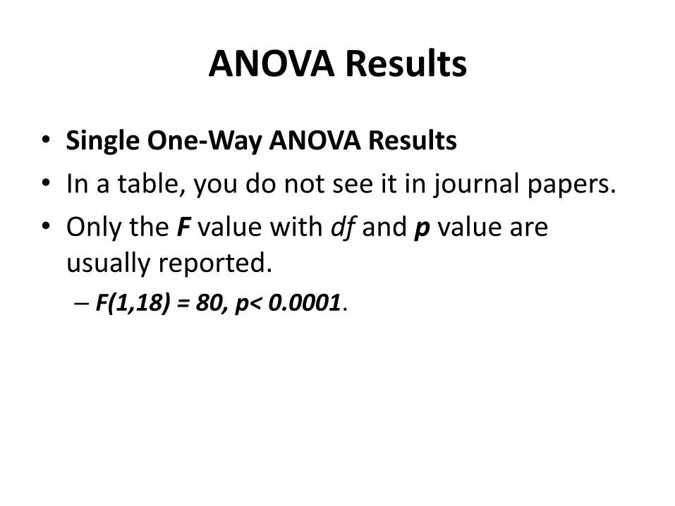
• Single One-Way ANOVA Results

• In a table, you do not see it in journal papers.

• Only the F value with df and p value are usually reported.

– F(1,18) = 80, p< 0.0001.

ANOVA Example

IQ Group1 IQ Group 2

123 78

123 33

111 23

113 45 101 54

103 34 99 61 89 45

110 65

105 65

Anova: Single Factor

SUMMARY

Groups Count Sum Average Variance

IQ Group1 10 1077 107.7 112.4556

IQ Group 2 10 503 50.3 299.3444

ANOVA

Source of Variation SS df MS F P-value F crit

Between Groups 16473.8 1 16473.8 80.00874 4.83E-08 4.413873

Within Groups 3706.2 18 205.9

Total 20180 19

Sum of Squares

Means Sum of squares =

SS /DF

The F statistic = Means Sum of Squares

(between) / Means Sum of Squares (within)

Differences between the averages for each

level

The variance within each level Degree of freedom: 1+1

= 2 Groups, 1+18+1= 20 subjects

ANOVA Results

• Two or more One-Way ANOVA Results

• Presented usually in the text.

• You should present:

– The independent variables.

– The F statistic

– The p value.

– And the degree of freedom.

• Readers will be able to know?

– The number of groups

– The number of subjects

– The independent variables

– The dependent variables

– The ….

Assumptions for a One-Way ANOVA

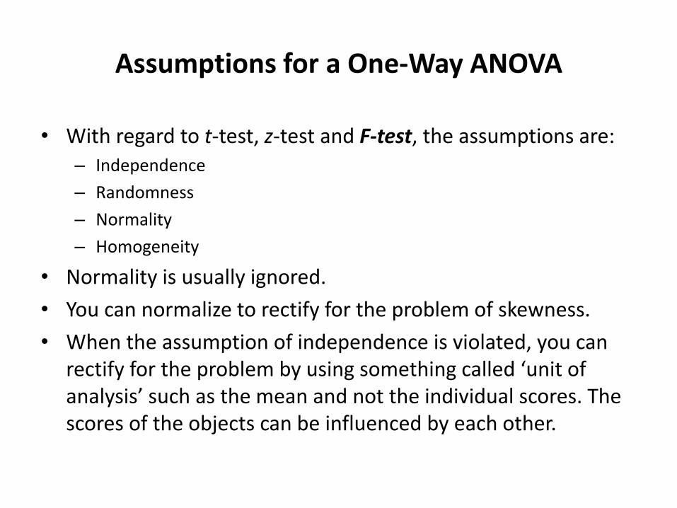
• With regard to t-test, z-test and F-test, the assumptions are: – Independence

– Randomness

– Normality

– Homogeneity

• Normality is usually ignored.

• You can normalize to rectify for the problem of skewness.

• When the assumption of independence is violated, you can rectify for the problem by using something called ‘unit of analysis’ such as the mean and not the individual scores. The scores of the objects can be influenced by each other.

Statistical vs. Practical Significance

• Again, effect size and post hoc power analysis can help with demonstrating the practical significance of the results.

• An a priori power analysis is rare but when used, the findings are much more convincing.

Warnings

• Statistically significant results mean rejecting the null hypothesis.

• ANOVA results does not provide information about how many µ values are dissimilar.

• It does not provide information about which two or more µ values are different.

• It only says that the variability among the samples’ means is larger than if the population

means were identical.

• One-Way ANOVA can be used with two means only.

• If confidence intervals are to be used, they should be build around each mean separately.

• There are some really good conclusions on PAGE 281 in the text book. Please read them

carefully.

Chapter 13

Two-Way Analysis of Variance

Two-Way Analysis of Variance

• Assumptions

– The populations from which the samples were obtained must be normally

or approximately normally distributed.

– The samples must be independent.

– The variances of the populations must be equal.

– The groups must have the same sample size.

– Source: http://people.richland.edu/james/lecture/m170/ch13-2wy.html

Two-Way ANOVA

• Involves two independent variables (factors).

• Only one dependent variable.

• One independent variable has factors (two or more)

and the other variable has levels (two or more).

• The combination of the factors and levels (cells) create

the conditions to be compared in the study.

Types of Factors

• Assigned: come as a result of the nature of the subject such as

gender and ethnicity.

• Active: Assigned by the researcher and it has to do with the

conditions of the study such as favorite food, willingness to die, and

so on.

• If the study has “all” assigned factors, the researcher will fill in the

ANOVA cells based on the characteristics of the subjects.

• If they were all active, they are controlled by the nature of the

study and assigned randomly into the cells.

Factors in a Two-Way ANOVA

• Can be described as:

– Between subjects: each group is measured under one

level of the factor.

– Within subjects: measured across all levels of the

factor.

• Usually assumed as between-subjects if not

stated explicitly.

Samples and Populations

• In a 3X2 ANOVA, the number of samples is

3*2=6.

• The number of populations is the same.

• In a study with two active factors, the

populations are abstract. Why?

Hypotheses

• The population means of the first factor are equal. This

is like the one-way ANOVA for the row factor.

• The population means of the second factor are equal.

This is like the one-way ANOVA for the column factor.

• There is no interaction between the two factors. This is

similar to performing a test for independence with

contingency tables.

Three Research Questions

• Is there a statistically significant main effect for the first factor (say rows for example)?

• Is there a statistically significant main effect for the second factor (say columns)?

• Is there a statistically significant interaction between the two factors?

Presentation of Results

• Two good examples of how to do ANOVA on excel.

– http://www.youtube.com/watch?v=F66weCUsRc0

– http://www.youtube.com/watch?v=STqxo4ToN18&feature=related

ANOVA in EXCEL

• Two-Way ANOVA with replication

• Two-Way ANOVA without replication

Data

Training Program 1 Training Program 2

Male

12 2

32 2

23 3 12 4 32 3

12 4 32 5

33 6

44 7 43 8

Female

12 33

11 23 9 24

4 25

5 25

34 43

4 23 5 43 7 44

9 7

Exam Scores (dependent

variable)

Two-Way ANOVA Results with replications

ANOVA

Source of Variation SS df MS F P-value F crit

Sample 126.025 1 126.025 1.357175 0.251689 4.113165

Columns 42.025 1 42.025 0.452571 0.505412 4.113165

Interaction 4431.025 1 4431.025 47.71812 4.34E-08 4.113165

Within 3342.9 36 92.85833

Total 7941.975 39

Two-Way ANOVA Results without replications

ANOVA

Source of Variation SS df MS F P-value F crit

Rows 2276.475 19 119.8145 0.404816 0.972183 2.168252

Columns 42.025 1 42.025 0.14199 0.710486 4.38075

Error (within groups) 5623.475 19 295.9724

Total 7941.975 39

Depicting Interaction

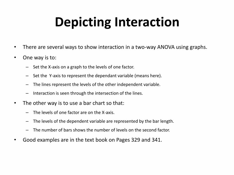
• There are several ways to show interaction in a two-way ANOVA using graphs.

• One way is to:

– Set the X-axis on a graph to the levels of one factor.

– Set the Y-axis to represent the dependant variable (means here).

– The lines represent the levels of the other independent variable.

– Interaction is seen through the intersection of the lines.

• The other way is to use a bar chart so that:

– The levels of one factor are on the X-axis.

– The levels of the dependent variable are represented by the bar length.

– The number of bars shows the number of levels on the second factor.

• Good examples are in the text book on Pages 329 and 341.

Post Hoc Tukey HSD and Scheffe

• Useful for demonstrating the practical significance of the results in case the statistical evidence does not lead to rejecting the null hypothesis.

• A good video: http://www.youtube.com/watch?v=rZuYwJupGus

Tukey HSD

• HSD stands for Honestly Significantly Different.

• More liberal than Scheffe.

• Tukey Test:

Level 1 Training

Level 2 Training

Level 3 Training

4 15 12

4 7 19

4 14 25

8 4 26

3 9 31

9 22 19

11 17 21

13 18 38

ANOVA

Source of Variation SS df MS F P-value F crit

Between Groups 1164.583 2 582.2917 15.05232 8.8E-05 3.4668

Within Groups 812.375 21 38.68452

Total 1976.958 23

Tukey Results