Tests on the CAPM

Introduction

We now give a conceptual overview of econometric techniquesused to test the CAPM.The overview follows the intellectual history of techniquedevelopment.We will return to the specifics of some of these techniques, andshow examples of usage.

Classical Empirical tests of the CAPM.

We cover the testing of the Capital Asset Pricing Model. Theperspective is the historical evolution of these tests, starting withthe classical papers and then looking at some of the importantimprovements in the testing methodology employed.

I Introductory.

I The relation between the conditional and unconditionalversions of the CAPM.

I Testable implications of the CAPM.I [Huang and Litzenberger, 1988, 10.7]

I Classical tests of the CAPM.I Fama and MacBeth [1973]I [Huang and Litzenberger, 1988, 10.13–10.16 (10.17-10.33 look

over.)]

I Multivariate tests. The following sets of papers improves onthe econometric testing methods.

I The Gibbons [1982] paper. Normality assumptions.I [Huang and Litzenberger, 1988, 10.34–10.40].I Gibbons et al. [1989].I MacKinlay and Richardson [1991]. GMM estimation

I Questioning the testability of the CAPM. The Roll Critique:Unobservability of the market portfolio.

I See [Huang and Litzenberger, 1988, 10.11,10.12]I The Stambaugh [1982] paper. Sensitivity of CAPM tests to

choice of benchmark.

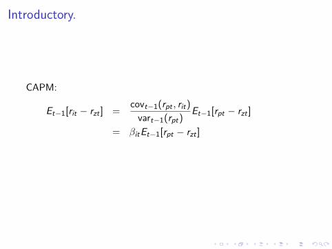
Introductory.

CAPM:

Et−1[rit − rzt ] =covt−1(rpt , rit)

vart−1(rpt)Et−1[rpt − rzt ]

= βitEt−1[rpt − rzt ]

conceptual

problems in testing the CAPM.

I The CAPM is an ex ante relation, not ex post.Assume rational expectations.

I CAPM is a static model, but we have a time series of data.We solve this by assuming that the CAPM holdsperiod-by-period. See the relation between conditional andunconditional restrictions.

I The market portfolio is unobservable. See Roll Critique

CAPM in conditional form

Et−1[rit − rzt ] = βitEt−1[rpt − rzt ] (1)

or, written explicitly

E [rit − rzt |Ωt−1] = βitE [rpt − rzt |Ωt−1]

This is assumed to hold over all possible information sets Ωt−1.By taking expectations over Ωt−1, we find that

E [E [rit − rzt |Ωt−1]] = E [βitE [rpt − rzt |Ωt−1]]

which implies that in unconditional expectations, the following isthe case

E [rit − rzt ] = βitE [rpt − rzt ] (2)

Justification for looking at the unconditional model.

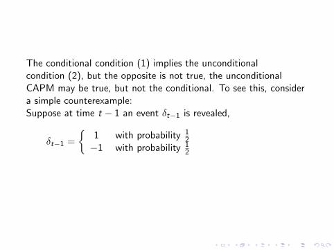
The conditional condition (1) implies the unconditionalcondition (2), but the opposite is not true, the unconditionalCAPM may be true, but not the conditional. To see this, considera simple counterexample:Suppose at time t − 1 an event δt−1 is revealed,

δt−1 =

1 with probability 1

2−1 with probability 1

2

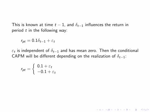
This is known at time t − 1, and δt−1 influences the return inperiod t in the following way:

rpt = 0.1δt−1 + εt

εt is independent of δt−1 and has mean zero. Then the conditionalCAPM will be different depending on the realization of δt−1:

rpt =

0.1 + εt−0.1 + εt

and

E [rpt ] =

0.1−0.1

with the conditional CAPM relations

E [rit − rzt |δt ] =

βip · (0.1− E [rzt |δt−1 = 1])βip · (−0.1− E [rzt |δt−1 = −1])

So, even if the unconditional expectation holds

E [rit − rzt ] = βip(E [rpt − rzt ])

this will not guarantee that the each of the conditionalexpectations hold...

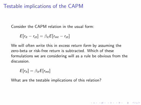
Testable implications of the CAPM

Consider the CAPM relation in the usual form:

E [rit − rzt ] = βitE [rmt − rzt ]

We will often write this in excess return form by assuming thezero-beta or risk-free return is subtracted. Which of theseformulations we are considering will as a rule be obvious from thediscussion.

E [rit ] = βitE [rmt ]

What are the testable implications of this relation?

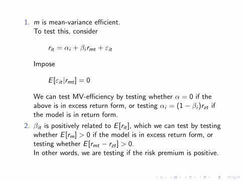
1. m is mean-variance efficient.To test this, consider

rit = αi + βi rmt + εit

Impose

E [εit |rmt ] = 0

We can test MV-efficiency by testing whether α = 0 if theabove is in excess return form, or testing αi = (1− βi )rzt ifthe model is in return form.

2. βit is positively related to E [rit ], which we can test by testingwhether E [rm] > 0 if the model is in excess return form, ortesting whether E [rmt − rzt ] > 0.In other words, we are testing if the risk premium is positive.

Classical tests

Tend to look at one return in isolation

The Fama and MacBeth [1973] paper.

Short summaryThis paper uses the Crossectional relation

(rjt − rft) = at + btβjm + ujt j = 1, 2, . . . ,N

Compare to the CAPM

rjt − rft = (rmt − rft)βjm

Prediction of the CAPM:

E [at ] = 0

E [bt ] = (E [rm]− rf ) > 0

To test this, average estimated at , bt :Test whether

E [at ] = 0,1

T

T∑t=1

at → 0

E [bt ] > 0,1

T

T∑t=1

bt > 0

To do these tests we need an estimate of βjm. The “usual”approach is to use time series data to estimate βjm from the“market model”

rjt = αj + βjmrmt + εjt

on data before the crossection.Results usually a > 0 and b > 0.

Looking at Fama and MacBeth [1973] paper.

The usual theoretical restriction:

E [Ri ] = E [R0] + βi (E [Rm]− E [R0])

Implications of the model tested in the paper:

C1: Risk-return relation is linear.

C2: βi is sufficient to describe expected return.

C3: Positive market premium.

Consider the multivariate regression:

Rit = γ0t + γ1tβi + γ2tβ2i + γ3tsi + ηit ,

where si is some measure of non-beta risk.What is actually tested?

C1: Linearity: Test γ2t = 0.

C2: βi sufficient: Test γ3t = 0.

C3: Positive market premium. Test γ1t > 0.

Note that these are test of the null against specific alternatives.

Implementation:I Control for nonstationarity of betas: Use portfolios instead of

individual securities.I βi is not known, replace with an estimate βi . How to get this

estimate? Implement by using data for previous periods to dobeta estimation, i.e. βit is estimated using return data forperiods t − 61 · · · t − 1.

I What to use as a measure of non-beta risk? In the paper,they estimate the (own) variance of the security.How do we find this estimate of the variance? Considerrunning a regression on the market, or the market model :

rit = αi + βi rmt + εit

In this context, the (own) variance is E [ε2it ]. FM uses theobvious estimate of the variance, by looking at the sampleanalogs of this for the same periods that the betas areestimated over.

sit =1

60

60∑j=1

(ri ,t−j − αi − βi rm,t−j

)2

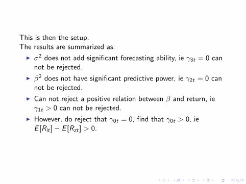
This is then the setup.The results are summarized as:

I σ2 does not add significant forecasting ability, ie γ3t = 0 cannot be rejected.

I β2 does not have significant predictive power, ie γ2t = 0 cannot be rejected.

I Can not reject a positive relation between β and return, ieγ1t > 0 can not be rejected.

I However, do reject that γ0t = 0, find that γ0t > 0, ieE [Rit ]− E [Rzt ] > 0.

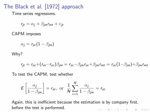
The Black et al. [1972] approachTime series regressions.

rjt = αj + βjmrmt + εjt

CAPM imposes

αj = rzc(1− βjm)

Why?

rjt = rzc+(rm−rzc)βjm = rzc−βjmrzc+βjmrmt = rzc(1−βjm)+βjmrmt

To test the CAPM, test whether

E

[αj

1− βjm

]= rzc , or

1

N

N∑i=1

αj

1− βjm= rzc

Again, this is inefficient because the estimation is by company first,before the test is performed.

A number of early test used a similar setup, and got similar results,well known examples are Blume and Friend [1973], Fama [1976]and Miller and Scholes [1972].Usually, the evidence of positivity of E [Rit ]− E [Rzt ] was viewed asevidence in favour of a constrained borrowing version of theCAPM, not necessarily a rejection of the model.What are the problems with the classical tests?Let us first look at two econometric problems, discussed incomprehensive detail in H&L 10.15 to 10.35.

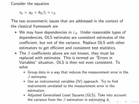
Consider the equation

rit = ait + bitβi + εit

The two econometric issues that are addressed in the context ofthe classical framework are

I We may have dependencies in εit . Under reasonable types ofdependencies, OLS estimates are consistent estimates of thecoefficient, but not of the variance. Replace OLS with otherestimators to get efficient and consistent test statistics.

I The β coefficients above are not known, they must bereplaced with estimates. This is termed an “Errors inVariables” situation. OLS is then not even consistent. Tosolve

I Group data in a way that reduces the measurement error in theβ estimates.

I Use an instrumental variables (IV) approach. Try to findinstruments unrelated to the measurement error in theestimation.

I Adjusted Generalised Least Squares (GLS). Take into accountthe variance from the β estimation in estimating b.

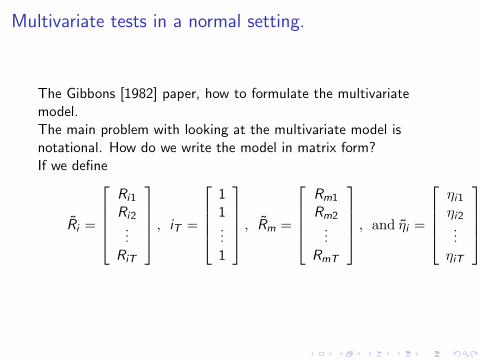
Multivariate tests in a normal setting.

The Gibbons [1982] paper, how to formulate the multivariatemodel.The main problem with looking at the multivariate model isnotational. How do we write the model in matrix form?If we define

Ri =

Ri1

Ri2...

RiT

, iT =

11...1

, Rm =

Rm1

Rm2...

RmT

, and ηi =

ηi1ηi2...ηiT

ηi is the error term, and in the paper this is assumedindependently, normally distributed (iidn).

ηi ∼ N (0, σii IT )

and we are looking at

Ri = αi + βi Rm + ηi

This is the same setup as in Black et al. [1972], and we have seenthat this imposes

Ri = rzc + βi (Rm − rzc) = rzc(1− βi ) + βi Rm

If the CAPM is true

Ri = rzc(1− βi ) + βi Rm

holds for all securities.If we estimate

Ri = αi + βi Rm + ηi

to test the CAPM, we test whether

H0 : αi = rzc(1− βi ) ∀ i

against

HA : αi 6= rzc(1− βi ) ∀ i

The problem is that we do not know rzc , it must be estimatedfrom the data. But then the estimation should take acount of that,under the null, rzc is the same across securities. It is thereforehelpful to stack the whole estimation into one set of equations.

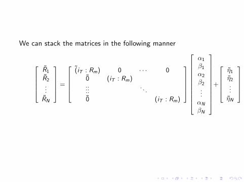
We can stack the matrices in the following manner

R1

R2

...

RN

=

(iT : Rm) 0 · · · 0

0 (iT : Rm)......

. . .

0 (iT : Rm)

α1

β1α2

β2...αN

βN

+

η1η2...ηN

and

(iT : Rm) =

1 Rm1

1 Rm2...1 RmT

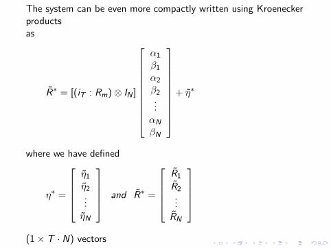
The system can be even more compactly written using Kroeneckerproductsas

R∗ = [(iT : Rm)⊗ IN ]

α1

β1α2

β2...αN

βN

+ η∗

where we have defined

η∗ =

η1η2...ηN

and R∗ =

R1

R2...

RN

(1× T · N) vectors

Kroenecker product ⊗:

A =

a11 a21 am1

a12 a22 am2

. . .

a1n amn

B =

b11 b21 bp1b12 b22 bp2

. . .

b1q bpq

A⊗ B =

a11B a21B am1Ba12B a22B am2B

. . .

a1nB amnB

A is a mp × nq matrix

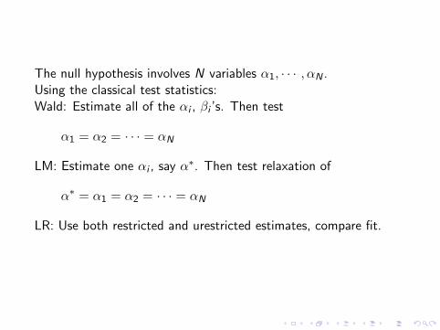
The null hypothesis involves N variables α1, · · · , αN .Using the classical test statistics:Wald: Estimate all of the αi , βi ’s. Then test

α1 = α2 = · · · = αN

LM: Estimate one αi , say α∗. Then test relaxation of

α∗ = α1 = α2 = · · · = αN

LR: Use both restricted and urestricted estimates, compare fit.

Multivariate test of the CAPM - GRSHowever, ideally want to use a test statistic to answer only onequestion, whether the market portfolio m mean variance efficient.If we use test on individual securities, we run a regression

rit = αi + βi rmt + εit

Then, by the CAPM, MV efficiency implies that

αi = rzt(1− βi )

for all securities i .One way to test MV efficiency would then be to testαi − rzt(1− βi ) = 0 for all the securities in the sample at (say) the5% level. The problem is then to aggregate this. Even if the null istrue, we expect to reject it in 5% of the cases. Seeing ifαi = rzt(1− βi ) for all i is of course one possibility, but this isextremely conservative. If we wanted to be less conservative, howmany rejections of the null for individual securities would we needto reject it for the market?

Hence, we are interested in aggregating over all assets in testingwhether the market portfolio m is M-V efficient.How to test for aggregate MV efficiency:Consider the estimation of the two following models:Unconstrained model

rjt = αj + βj rmt + ejt

Constrained model

rjt = rzt(1− βj) + βj rmt + ejt

The constrained model is a special case of the unconstrainedmodel.If the CAPM is true, and m is MV efficient, the constrained modelis the true model. Hence, our estimate of αj in the unconstrainedmodel should be approximately equal to rzt(1− βj) (the interceptin the constrained model)

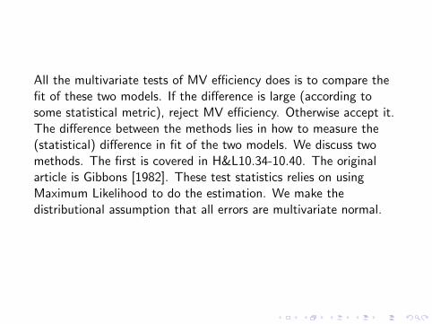
All the multivariate tests of MV efficiency does is to compare thefit of these two models. If the difference is large (according tosome statistical metric), reject MV efficiency. Otherwise accept it.The difference between the methods lies in how to measure the(statistical) difference in fit of the two models. We discuss twomethods. The first is covered in H&L10.34-10.40. The originalarticle is Gibbons [1982]. These test statistics relies on usingMaximum Likelihood to do the estimation. We make thedistributional assumption that all errors are multivariate normal.

Define:

rt =

r1t...rnt

αt =

α1t...αnt

βt =

β1t...βnt

and et =

e1t...ent

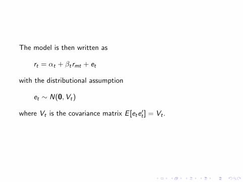
The model is then written as

rt = αt + βtrmt + et

with the distributional assumption

et ∼ N(0,Vt)

where Vt is the covariance matrix E [ete′t ] = Vt .

We find the estimates by maximising the log-likelihood `T withrespect to the parameters of interest.

`T = −(NT

2

)ln(2π)− T

2ln∣∣∣Ve

∣∣∣− 1

2

T∑t=1

e ′tV−1e et

We calculate the same function, but now using the estimates V ce

from the restricted model

`cT = −(NT

2

)ln(2π)− T

2ln∣∣∣V c

e

∣∣∣− 1

2

T∑t=1

ec′t (V ce )−1ect

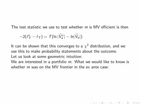
The test statistic we use to test whether m is MV efficient is then

−2(`cT − `T ) = T (ln |V ce | − ln|Ve |)

It can be shown that this converges to a χ2 distribution, and weuse this to make probability statements about the outcome.Let us look at some geometric intuition:We are interested in a portfolio m. What we would like to know iswhether m was on the MV frontier in the ex ante case:

6

-

E [r ]

σ

E [rz ]

E [rm]mr

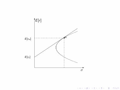
In ex post MV space, we can always form the ex post efficientfrontier:

6

-

r

σ

µz

µp

σp σm

prµm m

r

Here m is the ex post outcome for the portfolio m and p is an expost frontier portfolio. Intuitively, the test statistic measures thedifference in the slope of the two lines in the picture. If thisdifference is large, we think that the market portfolio is not ex anteefficient.

Multivariate test in a GMM setting.The test statistic in the Gibbons setting - developed underdistributional assumptions that allows using ML.What if these are not fulfilled, can we still construct a similar teststatistic?This is done in the paper of MacKinlay and Richardson [1991](MR). They construct a test statistic that essentially tests thesame restriction, that αi = E [rzt ](1− βi ), but in a GMMframework, not a ML.The setup is as follows.Again, we have the usual regression

rit = αi + βi rmt + εit

We assume that

E [εit |rmt ] = 0

This implies two moment restrictions for each asset i :

E [εit ] = E [(rit − αi − βi rmt)] = 0

E [εitrmt ] = E [(rit − αi − βi rmt)rmt ] = 0

The model is exactly identified. We can “stack” these momentconditions and estimate the parameters αi , βi of the model, bythe usual formulation using sample moments.The tests discussed in the paper are different ways of testing theparametric restriction αi = 0. Although they are implementeddifferently, they all give the same asymptotic result, only they havedifferent short-sample properties. There are three main types ofhypothesis tests (See Newey and West [1987])

I Wald-type: Estimate unconstrained model, test parameterrestriction.

I Lagrange-Multiplier type: Estimate constrained model, test fitof the (constrained) model.

I Likelihood Ratio type: Compare fit of the unconstrained andconstrained model.

Anomalies

Another challenge to the CAPM testing has come from theliteratur on anomalies. An anomaly is some observablecharacteristic of an asset that is not its beta and is useful inexplaining asset returns.The most famous anomalies is

I Firm size (Banz [1981]) and

I January.

The Roll critique.

the Roll critiqueRoll [1977] is concerned with the unobservability ofthe market portfolio, and its consequences for empirical testing.If we interpret the CAPM as an equilibrium model, the portfolio mis the return on all assets in the economy, not only the stockmarket indices we usually use as the market portfolio. Hence,rejecting/not rejecting the models in the tests above may not beviewed strictly as tests of the CAPM.One solution of this is to reinterpret the one-index formulation astests of a single factor APT.The usual way of addressing the problem is to assume that thestock market portfolio m is a sufficient statistic for the market. Letm be the market proxy and m the true, unobservable market. Ifρ(rm, rm) = 1, the beta estimates using m will be equal to the oneswe would have gotten using m.

The Stambaugh [1982] paper

So the assumption made is that the stock market index is “close”to the true market portfolio in the sense of having a unit betarelative to it.One paper that tries to look at how “close” the stock index is tothe “true” market empirically is Stambaugh [1982]. He adds alarge number of assets in addition to the stock market portfolio(bonds, real estate, household investment etc), and looks at thesensitivity of the conclusions of the empirical tests to whichportfolio is chosen.He finds that the conclusions are not sensitive to the assets in theportfolio, which makes us more confident about using only thestock market data. We may believe that the stock market index isa sufficient statistic for the whole market, or at least that itcaptures a good deal of the variability of the market as a whole.

Rolf W Banz. The relationship between return and market value of commonstocks. Journal of Financial Economics, 9:3–18, 1981.

Fisher Black, Michael Jensen, and Myron Scholes. The capital asset pricingmodel, some empirical tests. In Jensen [1972].

Marshall E Blume and I Friend. A new look at the capital asset pricing model.Journal of Finance, 28:19–33, 1973.

Eugene F Fama. Foundations of Finance. Basic Books, 1976.

Eugene F Fama and J MacBeth. Risk, return and equilibrium, empirical tests.Journal of Political Economy, 81:607–636, 1973.

Michael R Gibbons. Multivariate tests of financial models, a new approach.Journal of Financial Economics, 10:3–27, March 1982.

Michael R Gibbons, Stephen A Ross, and Jay Shanken. A test of the efficiencyof a given portfolio. Econometrica, 57:1121–1152, 1989.

Chi-fu Huang and Robert H Litzenberger. Foundations for financial economics.North–Holland, 1988.

Michael C Jensen, editor. Studies in the theory of capital markets. Preager,1972.

A Craig MacKinlay and Matthew P Richardson. Using generalized method ofmoments to test mean-variance efficiency. Journal of Finance, 46:511–27,1991.

Merton Miller and Myron Scholes. Rates of return in relation to risk, are-examination of some recent findings. In Jensen [1972].

Whitney K Newey and Kenneth D West. Hypothesis testing with efficientmethod of moments estimation. International Economic Review, 28:777–787, 1987.

Richard Roll. A critique of the asset pricing theory’s tests– Part I: On past andpotential testability of the theory. Journal of Financial Economics, 4:129–176, 1977.

Robert F Stambaugh. On the exlusion of assets from tests of thetwo-parameter model. Journal of Financial Economics, 10:237–268, 1982.