Tests for Random Numbers

Dr. Akram Ibrahim Aly

Lecture (9)

Tests for Random Numbers

• Frequency Tests: compare the distribution of the set of numbers to a uniform distribution– Kolmogorov-Smirnov (KS)– Chi-Square Test.

• Autocorrelation Test: Test the correlation between numbers and compares the sample correlation to the expected correlation of zero.

The Kolmogorov-Smirnov Test

• The KS test compares a continuous CDF F(x) to an empirical CDF SN(x), of the sample of N observations.

• If the sample from the random number generator is R1, R2, …, RN, then the empirical CDF SN(x) is given by:

N

x, R, , RRxS N

N

are which ofnumber )( 21

The Kolmogorov-Smirnov Test

• Step 1:– Rank the data from smallest to largest:

• Step 2:– Compute:

NRRR 21

i

NiR

N

iD

1max

N

iRD i

Ni

1max1

The Kolmogorov-Smirnov Test

• Step 3:– Compute D=max(D + ,D -)

• Step 4:– locate the critical value Dα in the “Kolmogorov Smirnov

Critical Values table” for the specified significance level α and the given sample size (N)

• Step 5:– If D ≤ Dα → Accept: “No difference between SN(x) and F(x)”

– If D > Dα → Reject: “No difference between SN(x) and F(x)”

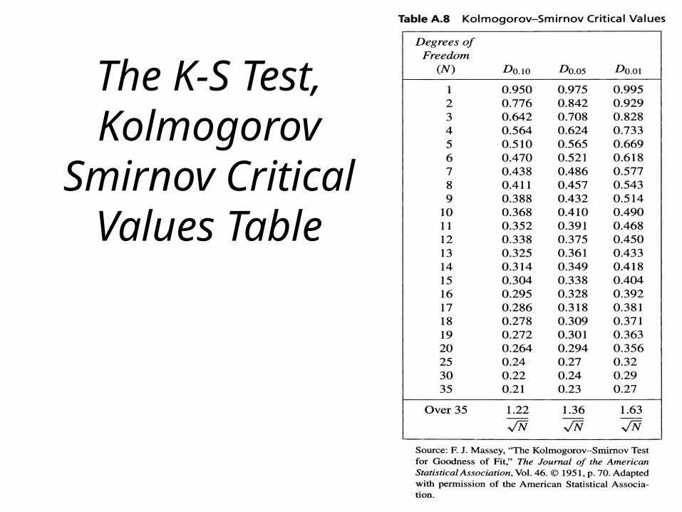
The K-S Test, Kolmogorov

Smirnov Critical Values Table

Example: The K-S Test

• The five numbers: 0.44, 0.81, 0.14, 0.05, 0.93 were generated and it is required to test for uniformity using the Kolmogorov-Smirnov Test with the level of significance α = 0.05.

Solution

0.05 0.14 0.44 0.81 0.93

0.2 0.4 0.6 0.8 1

0.15 0.26 0.16 -- 0.07

0.05 -- 0.04 0.21 0.13

• D=max(D +,D -) = max(0.26,0.21) = 0.26• In KS critical values table, For α = 0.05 and N = 5, the

critical value Dα= 0.565

• Since D < Dα , no difference has been detected between the true distribution of {R1, R2, …, RN} and the uniform distribution

iR

Ni

iRNi niRi 1

Solution: The K-S Test

The Chi-square Test

• The chi-square test uses the sample statistic:

• Where:– Oi = the number of observations in the i-th class

– Ei = the expected number in the i-th class

– n = the number of classes.

n

i i

ii

E

EO

1

220

The Chi-square Test

• Step 1:– Rank the data from smallest to largest:

• Step 2:– Divide the Range RN-R1 in n equidistant intervals

such that each interval has at least 5 observations.

• Step 3:– Calculate:

NRRR 21

n

i i

ii

E

EO

1

220

The Chi-square Test

• Step 4:– For significant level α, utilize the table of (Percentage

points of the chi square distribution with ν degrees of freedom) to determine χα,n-1.

• Step 5:– If χ0

2 ≤ χ2α,n-1 → Accept: “No difference between SN(x) and

F(x)”

– If χ02 > χ2

α,n-1 → Reject: “No difference between SN(x) and F(x)”

Example• Use the chi-square test with α=0.05 to test whether

the data shown next are uniformly distributed.

0.34 0.90 0.25 0.89 0.87 0.44 0.12 0.21 0.46 0.67

0.83 0.76 0.79 0.64 0.70 0.81 0.94 0.74 0.22 0.74

0.96 0.99 0.77 0.67 0.56 0.41 0.52 0.73 0.99 0.02

0.47 0.30 0.17 0.82 0.56 0.05 0.45 0.31 0.78 0.05

0.79 0.71 0.23 0.19 0.82 0.93 0.65 0.37 0.39 0.42

0.99 0.17 0.99 0.46 0.05 0.66 0.10 0.42 0.18 0.49

0.37 0.51 0.54 0.01 0.81 0.28 0.69 0.34 0.75 0.49

0.72 0.43 0.56 0.97 0.30 0.94 0.96 0.58 0.73 0.05

0.06 0.39 0.84 0.24 0.40 0.64 0.40 0.19 0.79 0.62

0.18 0.26 0.97 0.88 0.64 0.47 0.60 0.11 0.29 0.78

Solution

Interval

1 8 10 -2 4 0.4

2 8 10 -2 4 0.4

3 10 10 0 0 0

4 9 10 -1 1 0.1

5 12 10 2 4 0.4

6 8 10 -2 4 0.4

7 10 10 0 0 0

8 14 10 4 16 1.6

9 10 10 0 0 0

10 11 10 1 1 0.1

100 100 0 3.4

iO iE ii EO 2ii EO iii EEO 2

Solution

• The test uses n=10 intervals of equal length, namely [0,0.1[, [0.1,0.2[, …, [0.9,1]

• The value of χ02=3.4

• From table (Percentage points of the CHI SQUARE distribution with ν degrees of freedom), the critical value of χ0.05,9=16.9

• Since χ02< χ0.05,9, the hypothesis of uniform

distribution is not rejected.

Percentage points of the

CHI SQUARE distribution

with ν degrees of freedom

Notes on Uniformity tests

• Both the Kolmogorov-Smirnov test and the chi-square test are acceptable for testing the uniformity of sample data provided that the sample size is large.

• The KS test can be applied to small sample sizes, whereas the chi-square test is valid only for large samples, e.g.: N ≥ 50.

• The KS test is more powerful and is recommended

Test for Auto-correlation

• The tests for auto-correlation are concerned with the dependence between numbers in a sequence.

• Example:

– Examination of the 5th, 10th, 15th, …,etc. indicates a large number in that position.

0.12 0.01 0.23 0.28 0.89 0.31 0.64 0.28 0.83 0.93

0.99 0.15 0.33 0.35 0.91 0.41 0.60 0.27 0.75 0.88

0.68 0.49 0.05 0.43 0.95 0.58 0.19 0.36 0.69 0.87

Test for Auto-correlation

• The test requires the computation of the autocorrelation between every m numbers (m is known as the lag), starting with the ith number:– The autocorrelation ρim of interest shall be between

numbers: Ri, Ri+m, Ri+2m, Ri+(M+1)m

– M is the largest integer such that i+(M+1)m ≤ N

• If the values are uncorrelated:– For large values of M, the distribution of the estimator

of ρim , denoted is approximately normal.

Test for Auto-correlation• Test statistics is:

• Where:

• Z0 is distributed normally with mean = 0 and variance = 1.

112

713

25.01

1ˆ

ˆ

01

M

M

RRM

im

M

kmkikmiim

im

imZ

ˆ

0

ˆ

Test for Auto-correlation

• Compute Z0

• The hypothesis of independence is not rejected if:

• Where α is the level of significance and zα/2 is obtained from the standard normal distribution table.

2/02/ zZz

Test for Auto-correlation

• Figure illustrates the test

/ 2/ 2

-Z / 2 Z/ 2

Test for Auto-correlation

• If ρim> 0, the subsequence has positive autocorrelation– High random numbers tend to be followed by high

ones, and vice versa.

• If ρim< 0, the subsequence has negative autocorrelation– Low random numbers tend to be followed by high

ones, and vice versa.

Example

• Test whether the 3rd, 8th, 13th, and so on, for the following output using α = 0.05.

0.12 0.01 0.23 0.28 0.89 0.31 0.64 0.28 0.83 0.93

0.99 0.15 0.33 0.35 0.91 0.41 0.60 0.27 0.75 0.88

0.68 0.49 0.05 0.43 0.95 0.58 0.19 0.36 0.69 0.87

Solution

• i = 3, m = 5, N = 30,• 3+(M+1)5 ≤ 30→ M = 4•

•

1945.0ˆ

25.036.005.005.027.0

27.033.033.028.028.023.0

14

1ˆ

25.01

1ˆ

35

35

01

M

kmkikmiim RR

M

128.01412

7413

112

71335ˆ

M

M

Solution

• The test statistic is given by:

• From the standard normal distribution table, the critical value is:

• Since

• The hypothesis of independence cannot be rejected

1516.01280.0

1945.0ˆ

ˆ0

im

imZ

96.1025.02/05.0 zz

025.00025.0 zZz

The standard normal

distribution table