Testing Testing multifactor multifactor modelsmodels

EFM 2006/7EFM 2006/7 22

РЭШ

PlanPlan

Up to now:Up to now:– Testing CAPMTesting CAPM– Single pre-specified factorSingle pre-specified factor

Today:Today:– Testing multifactor modelsTesting multifactor models– The factors are unspecified!The factors are unspecified!

EFM 2006/7EFM 2006/7 33

РЭШ

Detailed planDetailed plan

Theoretical base for the multifactor Theoretical base for the multifactor models: APT and ICAPMmodels: APT and ICAPM

Testing when factors are traded Testing when factors are traded portfoliosportfolios

Statistical factorsStatistical factors Macroeconomic factorsMacroeconomic factors

– Chen, Roll, and Ross (1986)Chen, Roll, and Ross (1986) Fundamental factorsFundamental factors

– Fama and French (1993)Fama and French (1993)

EFM 2006/7EFM 2006/7 44

РЭШ

APTAPT

K-factor return-generating model for N assets:K-factor return-generating model for N assets:

RRtt = a + Bf = a + Bftt + ε + εtt,,– wwhere errors have zero expectation and are here errors have zero expectation and are

orthogonal to factorsorthogonal to factors– B is NxK matrix of factor loadingsB is NxK matrix of factor loadings

Cross-sectional equation for risk premiums: Cross-sectional equation for risk premiums:

E[R] = E[R] = λλ00ll + B + BλλKK

– wwhere here λλ is Kx1 vector of factor risk premiums is Kx1 vector of factor risk premiums ICAPM: another interpretation of factorsICAPM: another interpretation of factors

– The market ptf + state variables describing shifts in The market ptf + state variables describing shifts in the mean-variance frontierthe mean-variance frontier

EFM 2006/7EFM 2006/7 55

РЭШ

Specifics of testing Specifics of testing APTAPT No No need to estimate the market ptfneed to estimate the market ptf Can be estimated within a subset of the Can be estimated within a subset of the

assets assets Assume the Assume the exact exact form of APTform of APT

– In general, In general, approximate approximate APT, which is not APT, which is not testabletestable

The factors and their number are The factors and their number are unspecifiedunspecified– Factors can be traded portfolios or notFactors can be traded portfolios or not– Factors may explain cross differences in Factors may explain cross differences in

volatility, but have low risk premiumsvolatility, but have low risk premiums

EFM 2006/7EFM 2006/7 66

РЭШ

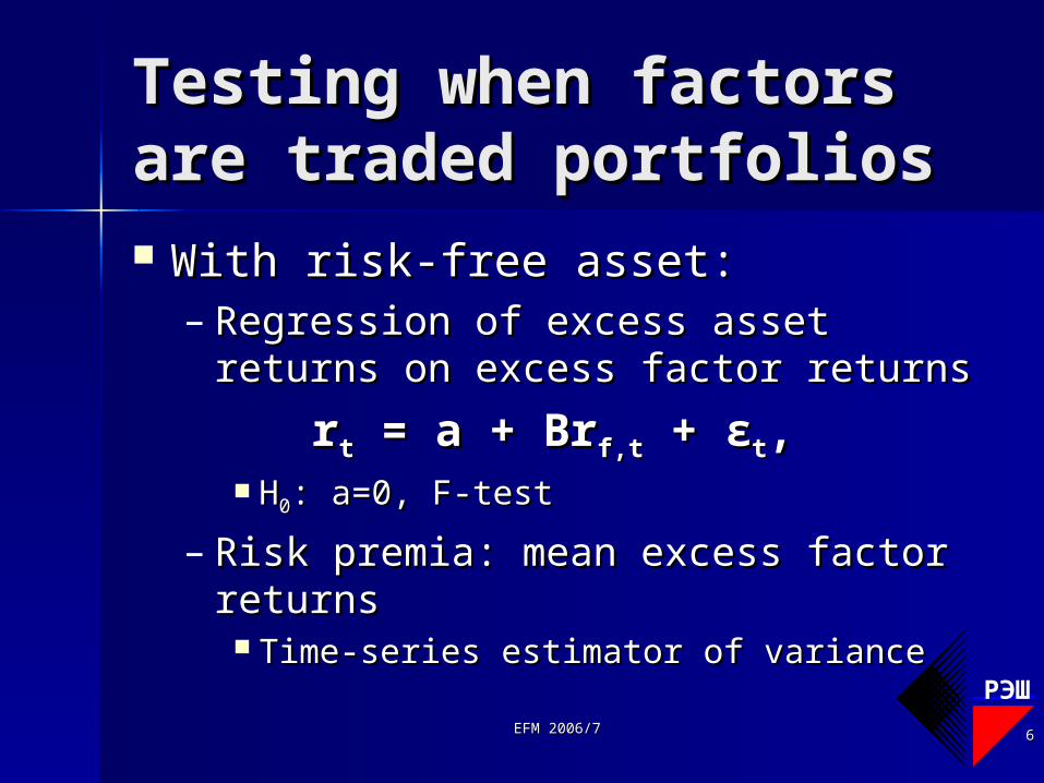
Testing when factors Testing when factors are traded portfoliosare traded portfolios With risk-free asset:With risk-free asset:

– Regression of excess asset returns Regression of excess asset returns on excess factor returnson excess factor returns

rrtt = a + Br = a + Brf,tf,t + ε + εtt,, HH00: a=0, F-test: a=0, F-test

– Risk premia: mean excess Risk premia: mean excess factor factor returnsreturns Time-series estimator of varianceTime-series estimator of variance

EFM 2006/7EFM 2006/7 77

РЭШ

Testing when factors Testing when factors are traded portfoliosare traded portfolios (cont.)(cont.) Without risk-free asset: need to estimate Without risk-free asset: need to estimate

zero-beta return zero-beta return γγ00

– Unconstrained regression of asset returns on Unconstrained regression of asset returns on factor returns:factor returns:

RRtt = a + B = a + BRRf,tf,t + + εεtt

– Constrained regression:Constrained regression:

RRtt = ( = (llNN-B-BllKK)γ)γ00 + BR + BRf,tf,t + + εεtt

– HH00: a=: a=((llNN-B-BllKK))γγ00, LR test , LR test – Risk premia: mean Risk premia: mean factor factor returns in excess of returns in excess of

γγ00 Variance is adjusted for the estimation error for Variance is adjusted for the estimation error for γγ00

EFM 2006/7EFM 2006/7 88

РЭШ

Testing when factors Testing when factors are traded portfoliosare traded portfolios (cont.)(cont.) When factor portfolios span the mean-When factor portfolios span the mean-

variance frontier: no need to specify variance frontier: no need to specify zero-beta assetzero-beta asset– Regression of asset returns on factor Regression of asset returns on factor

returns:returns:

RRtt = a + B = a + BRRf,tf,t + + εεtt

– HH00: a=0 and : a=0 and BBllKK==llNN Jensen’s alpha =0 & portfolio weights sum up Jensen’s alpha =0 & portfolio weights sum up

to 1to 1 Otherwise, factors do not span the MV frontier Otherwise, factors do not span the MV frontier

of the assets with returns Rof the assets with returns Rtt

EFM 2006/7EFM 2006/7 99

РЭШ

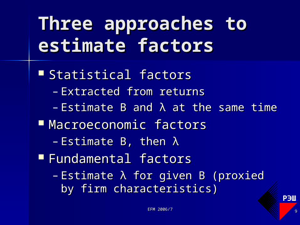
Three approaches to Three approaches to estimate factorsestimate factors Statistical factorsStatistical factors

– Extracted from returnsExtracted from returns– Estimate B and Estimate B and λλ at the same time at the same time

Macroeconomic factorsMacroeconomic factors– Estimate B, then Estimate B, then λλ

Fundamental factorsFundamental factors– Estimate Estimate λλ for given B (proxied by for given B (proxied by

firm characteristics)firm characteristics)

EFM 2006/7EFM 2006/7 1010

РЭШ

Statistical factors:Statistical factors: factor analysisfactor analysis

RRtt - μ- μ = Bf = Bftt + ε + εtt covcov(R(Rtt) = B ) = B ΩΩ B’ + D B’ + D

Assuming Assuming strict factor structurestrict factor structure: : – D≡cov(D≡cov(εεtt) is diagonal) is diagonal

Specification restrictions on factors: Specification restrictions on factors: – E(fE(ftt)=0, )=0, ΩΩ≡cov(f≡cov(ftt)=I)=I

Estimation:Estimation:– Estimate B and D by MLEstimate B and D by ML– Get fGet ftt from the cross-sectional GLS from the cross-sectional GLS

regression of asset returns on Bregression of asset returns on B

EFM 2006/7EFM 2006/7 1111

РЭШ

Statistical factors:Statistical factors: principal componentsprincipal components Classical approach: Classical approach:

– Choose linear combinations of asset Choose linear combinations of asset returns that maximize explained returns that maximize explained variancevariance

– Each subsequent component is Each subsequent component is orthogonal to the previous onesorthogonal to the previous ones

– Correspond to the largest Correspond to the largest eigenvectors of NxN eigenvectors of NxN matrix covmatrix cov(R(Rtt)) Rescaled s.t. weights sum up to 1Rescaled s.t. weights sum up to 1

EFM 2006/7EFM 2006/7 1212

РЭШ

Statistical factors:Statistical factors: principal componentsprincipal components Connor and Korajczyk (1988):Connor and Korajczyk (1988):

– Take K largest eigenvectors of TxT matrix r’r/NTake K largest eigenvectors of TxT matrix r’r/N where r is NxT excess return matrixwhere r is NxT excess return matrix

– As N→∞, KxT matrix of eigenvectors = factor As N→∞, KxT matrix of eigenvectors = factor realizationsrealizations

The factor estimates allow for time-varying risk The factor estimates allow for time-varying risk premiums!premiums!

– Refinement (like GLS): same for the Refinement (like GLS): same for the scaled scaled cross-product matrix cross-product matrix r’Dr’D-1r/Nr/N

where D has variances of the residuals from the first-where D has variances of the residuals from the first-stage ‘OLS’ on the diagonal, zeros off the diagonalstage ‘OLS’ on the diagonal, zeros off the diagonal

This increases the efficiency of the estimationThis increases the efficiency of the estimation

EFM 2006/7EFM 2006/7 1313

РЭШ

ResultsResults

5-6 factors are enough5-6 factors are enough– Based on explicit statistical tests Based on explicit statistical tests

and asset pricing testsand asset pricing tests Explain up to 40% of CS variation Explain up to 40% of CS variation

in stock returnsin stock returns– Better than CAPMBetter than CAPM

Explain some (January), but not Explain some (January), but not all (size, BE/ME) anomaliesall (size, BE/ME) anomalies

EFM 2006/7EFM 2006/7 1414

РЭШ

Discussion of Discussion of statistical factorsstatistical factors Missing economic interpretationMissing economic interpretation The explanatory power out of sample The explanatory power out of sample

is much lower than in-sampleis much lower than in-sample # factors rises with N# factors rises with N

– CK fix this problemCK fix this problem Static: slow reaction to the structural Static: slow reaction to the structural

changeschanges– Except for CK PCsExcept for CK PCs

EFM 2006/7EFM 2006/7 1515

РЭШ

Macroeconomic factorsMacroeconomic factors

Time series to estimate B:Time series to estimate B:

RRi,ti,t = a = aii + b’ + b’iifftt + + εεi,ti,t

Cross-sectional regressions to Cross-sectional regressions to estimate ex post risk premia for estimate ex post risk premia for each each tt::

RRi,ti,t = = λλ0,t0,t + b' + b'iiλλK,K,tt + e + ei,ti,t,,– Risk premia: mean and std from the Risk premia: mean and std from the

time series of ex post risk premia time series of ex post risk premia λλtt

EFM 2006/7EFM 2006/7 1616

РЭШ

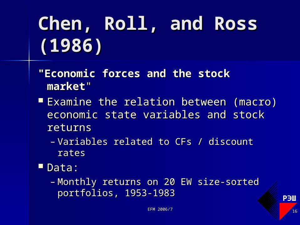
Chen, Roll, and Ross Chen, Roll, and Ross (1986)(1986)

"Economic forces and the stock "Economic forces and the stock marketmarket""

Examine the relation between Examine the relation between (macro) economic state variables and (macro) economic state variables and stock returnsstock returns– Variables related to CFs / discount ratesVariables related to CFs / discount rates

Data: Data: – Monthly returns on 20 EW size-sorted Monthly returns on 20 EW size-sorted

portfolios, 1953-1983portfolios, 1953-1983

EFM 2006/7EFM 2006/7 1717

РЭШ

Data: macro variablesData: macro variables

Industrial production growth: Industrial production growth: MPMPtt=ln(IP=ln(IPtt/IP/IPt-1t-1), ), YPYPtt=ln(IP=ln(IPtt/IP/IPt-12t-12))

Unanticipated inflation: Unanticipated inflation: UIUItt = I = Itt – E – Et-1t-1[I[Itt]] Change in expected inflation: Change in expected inflation: DEIDEItt = E = Ett[I[It+1t+1] – E] – Et-t-

11[I[Itt]] Default premium: Default premium: UPRUPRtt = Baa = Baatt – LGB – LGBtt

Term premium: Term premium: UTSUTStt = LGB = LGBtt – TB – TBt-1t-1

Real interest rate: RHOReal interest rate: RHOtt = TB = TBt-1t-1 – I – Itt

Market return: EWNYMarket return: EWNYtt and VWNY and VWNYtt (NYSE) (NYSE) Real consumption growth: CGReal consumption growth: CG Change in oil prices: OGChange in oil prices: OG

EFM 2006/7EFM 2006/7 1818

РЭШ

Methodology: Fama-Methodology: Fama-MacBeth procedureMacBeth procedure Each year, using 20 EW size-sorted Each year, using 20 EW size-sorted

portfolios:portfolios: Estimate factor loadings B from time-Estimate factor loadings B from time-

series regression, using previous 5 yearsseries regression, using previous 5 yearsRRi,ti,t = a = aii + b’ + b’iifftt + + εεi,ti,t

Estimate ex post risk premia from a Estimate ex post risk premia from a cross-sectional regression for each of cross-sectional regression for each of the next 12 monthsthe next 12 months

RRi,ti,t = = λλ0,t0,t + b' + b'iiλλK,K,tt + e + ei,ti,t,,– Risk premia: mean and std from the time Risk premia: mean and std from the time

series of ex post risk premia series of ex post risk premia λλtt

EFM 2006/7EFM 2006/7 1919

РЭШ

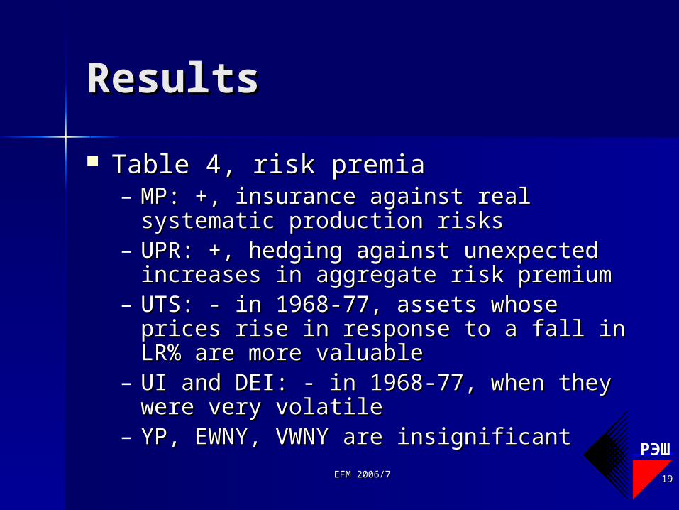
Results Results

Table 4, risk premiaTable 4, risk premia– MP: +, insurance against real systematic MP: +, insurance against real systematic

production risksproduction risks– UPR: +, hedging against unexpected UPR: +, hedging against unexpected

increases in aggregate risk premiumincreases in aggregate risk premium– UTS: - in 1968-77, assets whose prices UTS: - in 1968-77, assets whose prices

rise in response to a fall in LR% are more rise in response to a fall in LR% are more valuablevaluable

– UI and DEI: - in 1968-77, when they were UI and DEI: - in 1968-77, when they were very volatilevery volatile

– YP, EWNY, VWNY are insignificantYP, EWNY, VWNY are insignificant

EFM 2006/7EFM 2006/7 2020

РЭШ

Results (cont.)Results (cont.)

Table 5, risk premia when market Table 5, risk premia when market betas are estimated in univariate TS betas are estimated in univariate TS regressionregression– VWNY is significant when alone in CS VWNY is significant when alone in CS

regressionregression– VWNY is insignificant in the VWNY is insignificant in the

multivariate CS regressionmultivariate CS regression Tables 6 and 7, adding other Tables 6 and 7, adding other

variablesvariables– CG is insignificantCG is insignificant– OG: + in 1958-67OG: + in 1958-67

EFM 2006/7EFM 2006/7 2121

РЭШ

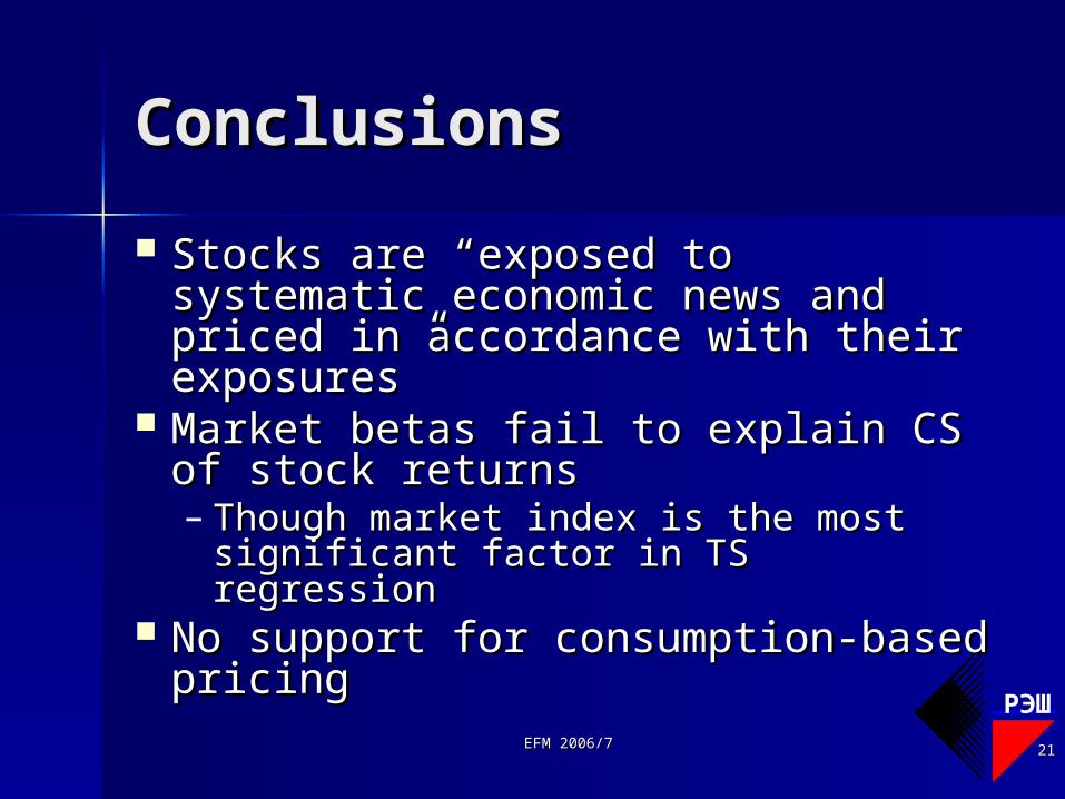
ConclusionsConclusions

Stocks are “exposed to Stocks are “exposed to systematic economic news and systematic economic news and priced in accordance with their priced in accordance with their exposures”exposures”

Market betas fail to explain CS of Market betas fail to explain CS of stock returnsstock returns– Though market index is the most Though market index is the most

significant factor in TS regressionsignificant factor in TS regression No support for consumption-No support for consumption-

based pricingbased pricing

EFM 2006/7EFM 2006/7 2222

РЭШ

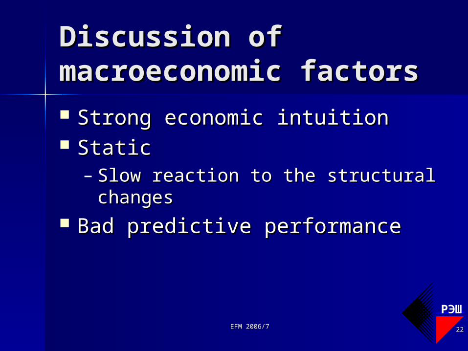
DiscussionDiscussion of of macroeconomic factorsmacroeconomic factors Strong economic intuitionStrong economic intuition StaticStatic

– Slow reaction to the structural Slow reaction to the structural changeschanges

Bad predictive performanceBad predictive performance

EFM 2006/7EFM 2006/7 2323

РЭШ

Fundamental factorsFundamental factors

B is proxied by firm characteristics:B is proxied by firm characteristics:– Market cap, leverage, E/P, liquidity, etc.Market cap, leverage, E/P, liquidity, etc.– Taken from CAPM violationsTaken from CAPM violations

Cross-sectional regressions for each Cross-sectional regressions for each tt to to estimate risk premia:estimate risk premia:

RRi,ti,t = = λλ0,t0,t + b' + b'iiλλK,K,tt + e + ei,ti,t Alternative: Alternative: factor-mimicking portfoliosfactor-mimicking portfolios

– Zero-investment portfolios: long/short Zero-investment portfolios: long/short position in stocks with high/low value of the position in stocks with high/low value of the attributeattribute

EFM 2006/7EFM 2006/7 2424

РЭШ

Fama and FrenchFama and French (1993)(1993)"Common risk factors in the returns "Common risk factors in the returns

on stocks and bondson stocks and bonds"" Identify risk factors in stock and bond Identify risk factors in stock and bond

marketsmarkets– Factors for stocks are size and book-to-Factors for stocks are size and book-to-

marketmarket In contrast to Fama&French (1992): In contrast to Fama&French (1992): time time

series series teststests

– Factors for bonds are term structure Factors for bonds are term structure variablesvariables

– Links between stock and bond factorsLinks between stock and bond factors

EFM 2006/7EFM 2006/7 2525

РЭШ

DataData

All non-financial firms in NYSE, All non-financial firms in NYSE, AMEX, and (after 1972) NASDAQ in AMEX, and (after 1972) NASDAQ in 1963-19911963-1991

Monthly return data (CRSP)Monthly return data (CRSP) Annual financial statement data Annual financial statement data

(COMPUSTAT)(COMPUSTAT)– Used with a 6m gapUsed with a 6m gap

Market index: the CRSP value-wtd Market index: the CRSP value-wtd portfolio of stocks in the three portfolio of stocks in the three exchangesexchanges

EFM 2006/7EFM 2006/7 2626

РЭШ

MethodologyMethodology

Stock market factors:Stock market factors:– Market: RM-RFMarket: RM-RF– Size: MESize: ME– Book-to-market equity: BE/MEBook-to-market equity: BE/ME

Bond market factors:Bond market factors:– TERM = (Return on Long-term Gvt TERM = (Return on Long-term Gvt

Bonds) – (T-bill rate)Bonds) – (T-bill rate)– DEF = (Return on Corp Bonds) – DEF = (Return on Corp Bonds) –

(Return on Long-term Gvt Bonds)(Return on Long-term Gvt Bonds)

EFM 2006/7EFM 2006/7 2727

РЭШ

Constructing factor-Constructing factor-mimicking portfoliosmimicking portfolios In June of each year In June of each year tt, break stocks into:, break stocks into:

– Two size groups: Small / Big (below/above Two size groups: Small / Big (below/above median)median)

– Three BE/ME groups: Low (bottom 30%) / Three BE/ME groups: Low (bottom 30%) / Medium / High (top 30%)Medium / High (top 30%)

– Compute monthly VW returns of 6 size-BE/ME Compute monthly VW returns of 6 size-BE/ME portfolios for the next 12 monthsportfolios for the next 12 months

Factor-mimicking portfolios: zero-investmentFactor-mimicking portfolios: zero-investment– Size: Size: SMBSMB = 1/3(SL+SM+SH) – = 1/3(SL+SM+SH) –

1/3(BL+BM+BH)1/3(BL+BM+BH)– BE/ME: BE/ME: HMLHML = 1/2(BH+SH) – 1/2(BL+SL) = 1/2(BH+SH) – 1/2(BL+SL)

EFM 2006/7EFM 2006/7 2828

РЭШ

The returns to be The returns to be explainedexplained 25 stock portfolios25 stock portfolios

– In June of each year In June of each year tt, stocks are sorted by size , stocks are sorted by size (current ME) and (independently) by BE/ME (as of (current ME) and (independently) by BE/ME (as of December of December of tt-1)-1)

– Using NYSE quintile breakpoints, all stocks are Using NYSE quintile breakpoints, all stocks are allocated to one of 5 size portfolios and one of 5 allocated to one of 5 size portfolios and one of 5 BE/ME portfoliosBE/ME portfolios

– From July of From July of tt to June of to June of tt+1, monthly VW returns +1, monthly VW returns of 25 size-BE/ME portfolios are computedof 25 size-BE/ME portfolios are computed

7 bond portfolios7 bond portfolios– 2 gvt portfolios: 1-5y, 6-10y maturity2 gvt portfolios: 1-5y, 6-10y maturity– 5 corporate bond portfolios: Aaa, Aa, A, Baa, 5 corporate bond portfolios: Aaa, Aa, A, Baa,

below Baabelow Baa

EFM 2006/7EFM 2006/7 2929

РЭШ

Time-series testsTime-series tests

Regressions of excess asset Regressions of excess asset returns on factor returns:returns on factor returns:

rri,ti,t = a = aii + b’ + b’iirrf,tf,t + + εεi,ti,t

– Common variation: slopes and RCommon variation: slopes and R22

– Pricing: interceptsPricing: intercepts

EFM 2006/7EFM 2006/7 3030

РЭШ

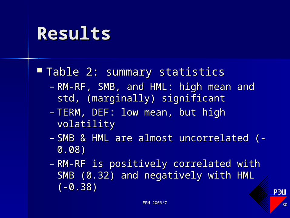
ResultsResults

Table 2: summary statisticsTable 2: summary statistics– RM-RF, SMB, and HML: high mean and RM-RF, SMB, and HML: high mean and

std, (marginally) significantstd, (marginally) significant– TERM, DEF: low mean, but high TERM, DEF: low mean, but high

volatilityvolatility– SMB & HML are almost uncorrelated (-SMB & HML are almost uncorrelated (-

0.08)0.08)– RM-RF is positively correlated with SMB RM-RF is positively correlated with SMB

(0.32) and negatively with HML (-0.38)(0.32) and negatively with HML (-0.38)

EFM 2006/7EFM 2006/7 3131

РЭШ

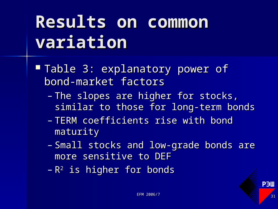
Results on common Results on common variationvariation Table 3: explanatory power of Table 3: explanatory power of

bond-market factorsbond-market factors– The slopes are higher for stocks, The slopes are higher for stocks,

similar to those for long-term bondssimilar to those for long-term bonds– TERM coefficients rise with bond TERM coefficients rise with bond

maturitymaturity– Small stocks and low-grade bonds are Small stocks and low-grade bonds are

more sensitive to DEFmore sensitive to DEF– RR22 is higher for bonds is higher for bonds

EFM 2006/7EFM 2006/7 3232

РЭШ

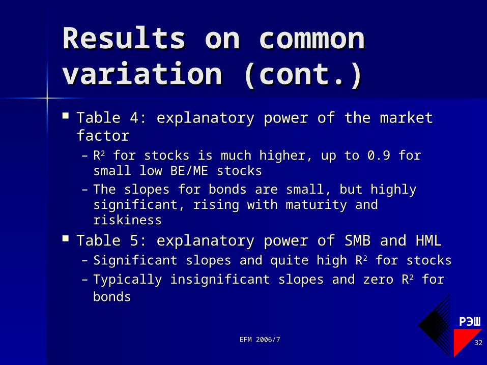
Results on common Results on common variationvariation (cont.)(cont.) Table 4: explanatory power of the market Table 4: explanatory power of the market

factorfactor– RR22 for stocks is much higher, up to 0.9 for small for stocks is much higher, up to 0.9 for small

low BE/ME stockslow BE/ME stocks– The slopes for bonds are small, but highly The slopes for bonds are small, but highly

significant, rising with maturity and riskinesssignificant, rising with maturity and riskiness Table 5: explanatory power of SMB and Table 5: explanatory power of SMB and

HMLHML– Significant slopes and quite high RSignificant slopes and quite high R22 for stocks for stocks– Typically insignificant slopes and zero RTypically insignificant slopes and zero R22 for for

bondsbonds

EFM 2006/7EFM 2006/7 3333

РЭШ

Results on common Results on common variationvariation (cont.)(cont.) Table 6: explanatory power of RM-RF, SMB and Table 6: explanatory power of RM-RF, SMB and

HMLHML– Slopes for stocks are highly significant, RSlopes for stocks are highly significant, R22 is typically is typically

over 0.9over 0.9– Market betas move toward oneMarket betas move toward one– The SMB and HML slopes for bonds become significantThe SMB and HML slopes for bonds become significant

Table 7: five-factor regressionsTable 7: five-factor regressions– Stocks: stock factors remain significant, but kill Stocks: stock factors remain significant, but kill

significance of bond factorssignificance of bond factors– Bonds: bond factors remain significant, stock factors Bonds: bond factors remain significant, stock factors

become much less importantbecome much less important RM-RF help to explain high-grade bondsRM-RF help to explain high-grade bonds SMB and HML help to explain low-grade bondsSMB and HML help to explain low-grade bonds

EFM 2006/7EFM 2006/7 3434

РЭШ

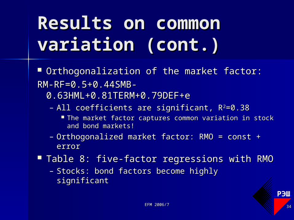
Results on common Results on common variationvariation (cont.)(cont.) Orthogonalization of the market factor:Orthogonalization of the market factor:

RM-RF=0.5+0.44SMB-RM-RF=0.5+0.44SMB-0.63HML+0.81TERM+0.79DEF+e0.63HML+0.81TERM+0.79DEF+e– All coefficients are significant, RAll coefficients are significant, R22=0.38=0.38

The market factor captures common variation in The market factor captures common variation in stock and bond markets!stock and bond markets!

– Orthogonalized market factor: RMO = const + Orthogonalized market factor: RMO = const + errorerror

Table 8: five-factor regressions with RMOTable 8: five-factor regressions with RMO– Stocks: bond factors become highly significantStocks: bond factors become highly significant

EFM 2006/7EFM 2006/7 3535

РЭШ

Results on pricingResults on pricing

Table 9a, stocksTable 9a, stocks– TERM, DEF: positive interceptsTERM, DEF: positive intercepts– RM-RF: size effectRM-RF: size effect– SMB, HML: big positive interceptsSMB, HML: big positive intercepts– RM-RF, SMB, HML: most intercepts RM-RF, SMB, HML: most intercepts

are 0are 0– Adding bond factors does not Adding bond factors does not

improveimprove

EFM 2006/7EFM 2006/7 3636

РЭШ

Results on pricingResults on pricing (cont.)(cont.) Table 9b, bondsTable 9b, bonds

– TERM, DEF: positive intercepts for gvt TERM, DEF: positive intercepts for gvt bondsbonds

– RM-RF or SMB with HML make intercepts RM-RF or SMB with HML make intercepts insignificantinsignificant

– Increased precision due to TERM and DEF Increased precision due to TERM and DEF explains positive intercepts in a five-factor explains positive intercepts in a five-factor modelmodel

Table 9c, F-testTable 9c, F-test– Joint test for zero intercepts rejects the null Joint test for zero intercepts rejects the null

for all modelsfor all models– The best model for stocks is a model with The best model for stocks is a model with

three stock factorsthree stock factors

EFM 2006/7EFM 2006/7 3737

РЭШ

DiagnosticsDiagnostics

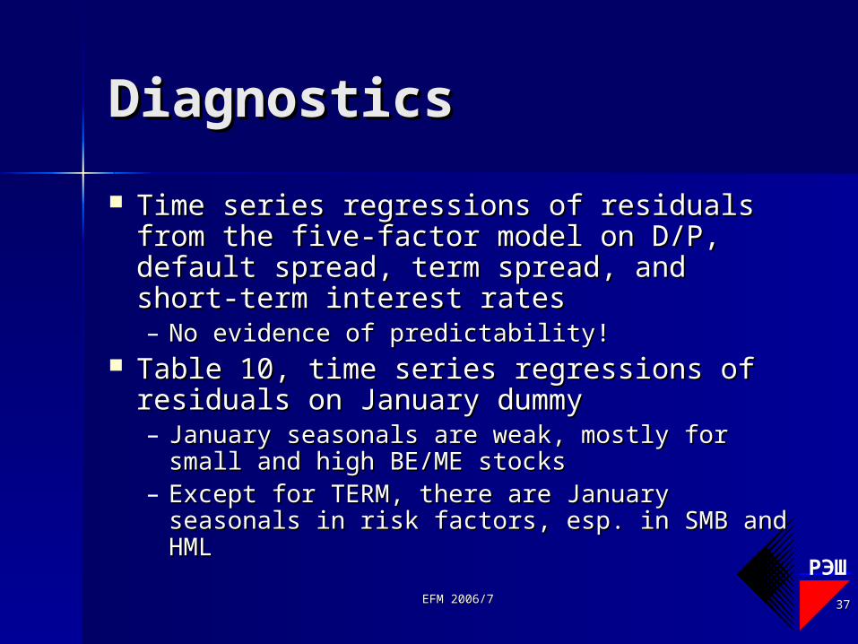
Time series regressions of residuals from Time series regressions of residuals from the five-factor model on D/P, default the five-factor model on D/P, default spread, term spread, and short-term spread, term spread, and short-term interest ratesinterest rates– No evidence of predictability!No evidence of predictability!

Table 10, time series regressions of Table 10, time series regressions of residuals on January dummyresiduals on January dummy– January seasonals are weak, mostly for small January seasonals are weak, mostly for small

and high BE/ME stocksand high BE/ME stocks– Except for TERM, there are January seasonals Except for TERM, there are January seasonals

in risk factors, esp. in SMB and HMLin risk factors, esp. in SMB and HML

EFM 2006/7EFM 2006/7 3838

РЭШ

Split-sample testsSplit-sample tests

Each of the size-BE/ME portfolios Each of the size-BE/ME portfolios is split into two halvesis split into two halves– One is used to form factorsOne is used to form factors– Another is used as dependent Another is used as dependent

variables in regressionsvariables in regressions Similar resultsSimilar results

EFM 2006/7EFM 2006/7 3939

РЭШ

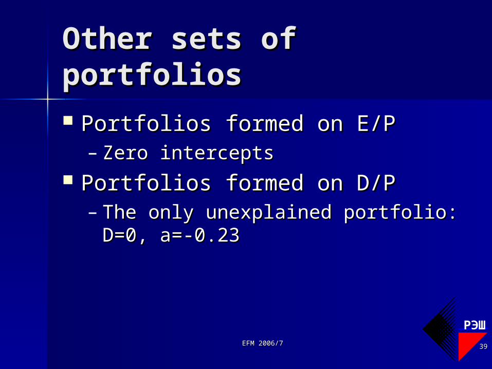
Other sets of Other sets of portfoliosportfolios Portfolios formed on E/PPortfolios formed on E/P

– Zero interceptsZero intercepts Portfolios formed on D/PPortfolios formed on D/P

– The only unexplained portfolio: The only unexplained portfolio: D=0, a=-0.23D=0, a=-0.23

EFM 2006/7EFM 2006/7 4040

РЭШ

ConclusionsConclusions

There is an overlap between processes in stock There is an overlap between processes in stock and bond marketsand bond markets– Bond market factors capture common variation in stock Bond market factors capture common variation in stock

and bond returns, though explain almost no average and bond returns, though explain almost no average excess stock returnsexcess stock returns

Three-factor model with the market, size, and Three-factor model with the market, size, and book-to-market factors explains well stock returnsbook-to-market factors explains well stock returns– SMB and HML explain the cross differencesSMB and HML explain the cross differences– RM-RF explains why stock returns are on average above RM-RF explains why stock returns are on average above

the T-bill ratethe T-bill rate Two bond factors explain well variation in bond Two bond factors explain well variation in bond

returnsreturns– SMB and HML help to explain variation of low-grade SMB and HML help to explain variation of low-grade

bondsbonds

EFM 2006/7EFM 2006/7 4141

РЭШ

Fama and FrenchFama and French (1995)(1995)"Size and book-to-market factors in "Size and book-to-market factors in

earnings and returnsearnings and returns"" There are size and book-to-market factors There are size and book-to-market factors

in earnings which proxy for relative in earnings which proxy for relative distressdistress– Strong firms with persistently high earnings Strong firms with persistently high earnings

have low BE/MEhave low BE/ME– Small stocks tend to be less profitableSmall stocks tend to be less profitable

There is some relation between common There is some relation between common factors in earnings and return variationfactors in earnings and return variation

EFM 2006/7EFM 2006/7 4242

РЭШ

Fama and FrenchFama and French (1996)(1996)"Multifactor explanations of asset pricing "Multifactor explanations of asset pricing

anomaliesanomalies"" Run time-series regressions for decile portfolios Run time-series regressions for decile portfolios

based on sorting by E/P, C/P, sales, past returnsbased on sorting by E/P, C/P, sales, past returns– The three-factor model explains all anomalies but one-year The three-factor model explains all anomalies but one-year

momentum effectmomentum effect Interpretation of the three-factor model in terms of Interpretation of the three-factor model in terms of

the underlying portfolios M, S, B, H, and L: the underlying portfolios M, S, B, H, and L: spanning testsspanning tests– M and B are highly correlated (0.99)M and B are highly correlated (0.99)– Excess returns of any three of M, S, H, and L explain the Excess returns of any three of M, S, H, and L explain the

fourthfourth– Different triplets of the excess returns for M, S, H, and L Different triplets of the excess returns for M, S, H, and L

provide similar results in explaining stock returnsprovide similar results in explaining stock returns This is taken as evidence of multifactor ICAPM or This is taken as evidence of multifactor ICAPM or

APTAPT

EFM 2006/7EFM 2006/7 4343

РЭШ

DiscussionDiscussion of of fundamental factorsfundamental factors High predictive powerHigh predictive power DynamicDynamic Though: data-intensiveThough: data-intensive Widely applied:Widely applied:

– Portfolio selection and risk managementPortfolio selection and risk management– Performance evaluationPerformance evaluation– Measuring abnormal returns in event Measuring abnormal returns in event

studiesstudies– Estimating the cost of capitalEstimating the cost of capital