Testing if the market microstructure noise is fully explained by theinformational content of some variables from the limit order book∗

Simon Clinet†‡and Yoann Potiron§

This version: June 29, 2018

Abstract

In this paper, we build tests for the presence of residual noise in a model where the marketmicrostructure noise is a known parametric function of some variables from the limit order book.The tests compare two distinct quasi-maximum likelihood estimators of volatility, where the relatedmodel includes a residual noise in the market microstructure noise or not. The limit theory isinvestigated in a general nonparametric framework. In the presence of residual noise, we examinethe central limit theory of the related quasi-maximum likelihood estimation approach.

Keywords: efficient price ; estimation ; high frequency data ; information ; limit order book ; marketmicrostructure noise ; integrated volatility ; quasi-maximum likelihood estimator ; realized volatility ;test

1 Introduction

If one can sample directly from the efficient price, the estimation of volatility is a well-studied matter.The realized volatility (RV) estimator, i.e. summing the square of the log-returns, is both consistentand efficient. However, in practice the observed price does not behave as expected. When sampling athigh frequency, it can be quite different from the efficient price due to bid-ask bounce mechanism, the∗We would like to thank Yingying Li, Xinghua Zheng, Dacheng Xiu, Viktor Todorov, Torben Andersen, Rasmus

Varneskov, Rui Da, Yacine Aït-Sahalia (the Editor), two anonymous referees and an anonymous Associate Editor, theparticipants of ECOSTA 2018, 2018 Asian meeting of the Econometric Society, SoFiE Financial Econometrics SummerSchool 2017 at Kellogg School of Management and 2017 Asian meeting of the Econometric Society at The ChineseUniversity of Hong Kong for helpful discussions and advice. The research of Yoann Potiron is supported by JapaneseSociety for the Promotion of Science Grant-in-Aid for Young Scientists (B) No. 60781119 and a special grant from KeioUniversity. The research of Simon Clinet is supported by CREST Japan Science and Technology Agency and a specialgrant from Keio University.†Faculty of Economics, Keio University. 2-15-45 Mita, Minato-ku, Tokyo, 108-8345, Japan. Phone: +81-3-5427-1506.

E-mail: clinet@keio.jp website: http://user.keio.ac.jp/~clinet‡CREST, Japan Science and Technology Agency, Japan.§Faculty of Business and Commerce, Keio University. 2-15-45 Mita, Minato-ku, Tokyo, 108-8345, Japan. Phone:

+81-3-5418-6571. E-mail: potiron@fbc.keio.ac.jp website: http://www.fbc.keio.ac.jp/~potiron

1

arX

iv:1

709.

0250

2v3

[q-

fin.

ST]

28

Jun

2018

spread, the fact that transactions lie on a tick grid, etc. Market microstructure noise (MMN) typicallydegrades RV to the extent that it is highly biased when performed on tick by tick data.

One approach to overcome the problem consists in sub-sampling, say every 5 minutes, as in thepioneer work from [Andersen et al., 2001] and [Barndorff-Nielsen and Shephard, 2002]. On the con-trary, [Aït-Sahalia et al., 2005] recognize the MMN as an inherent part of the data and advice forthe use of the Quasi-Maximum Likelihood Estimator (QMLE) which was later shown to be robustto time-varying volatility in [Xiu, 2010]. Concurrent methods include and are not limited to: theTwo-Scale Realized Volatility (TSRV) in [Zhang et al., 2005], the Multi-Scale Realized Volatility in[Zhang, 2006], the Pre-averaging approach (PAE) in [Jacod et al., 2009], realized kernels (RK) in[Barndorff-Nielsen et al., 2008] and the spectral approach considered in [Altmeyer and Bibinger, 2015].

Those two approaches have cons in that the sub-sampling technique discards a large proportion ofthe data and the noise-robust estimators have a slower rate of convergence than RV. In this paper, weconsider the MMN as a salient part of the financial market, but using the growing limit order book(LOB) big data available to the econometrician we ask a different question. Can we test whether theMMN is fully explained by the informational content of some variables from the limit order book andcan we estimate the parameter of the model? If the MMN can be expressed as an observable function,then we can estimate the efficient price and use RV including all the data points. This idea is not new,and actually our work is heavily based on the two very nice papers [Li et al., 2016] and [Chaker, 2017].We will explain the differences later in the introduction.

In fact it is rather natural to see the MMN as a function of some variables of the LOB as in thepioneer work from [Roll, 1984] where the trade type, i.e. whether the trade was buyer or seller initiated,is used to correct for the bid ask bounce effect in the observed price. The related observed price Zti isthen defined as

Zti︸︷︷︸observed price

= Xti︸︷︷︸efficient price

+ Iiθ0︸︷︷︸MMN

, (1.1)

where θ0 can be interpreted as one-half of the effective bid-ask spread, Ii is equal to 1 if the trade at timeti is buyer-initiated and -1 if seller-initiated. A simple extension where the spread Si is time-varyingis given by

Zti = Xti +1

2IiSiθ0. (1.2)

Discussion and related leading models can be found in: [Black, 1986], [Hasbrouck, 1993], [O’hara, 1995],[Madhavan et al., 1997], [Madhavan, 2000], [Stoll, 2000] and [Hasbrouck, 2007] among other prominentwork.

The question we address is: can we trust models such as (1.1) or (1.2)? To investigate it, weintroduce the general set-up as

Zti︸︷︷︸observed price

= Xti︸︷︷︸efficient price

+ φ(Qi, θ0)︸ ︷︷ ︸explicative part

+ εti︸︷︷︸residual noise︸ ︷︷ ︸

MMN

, (1.3)

2

where Qi are observable variables included in the LOB while φ is known to the econometrician, and wedevelop tests for the presence of the residual noise εti at any given sampling frequency. The associatednull hypothesis is such that εti = 0, φ = Φ and the alternative Var[εti ] > 0, φ = Φ or φ = 0, whereΦ := Φ(Qi, θ0) 6= 0 is known up to the parameter θ0.

Our tests are based on [Hausman, 1978] tests1 developed in [Aït-Sahalia and Xiu, 2016], whichis restricted to the case Φ = 0. The authors consider the difference σ2

RV − σ2QMLE , where σ

2RV =

T−1∑

i(Zti−Zti−1)2 and σ2QMLE corresponds to the QMLE in a model where φ = 0. The Hausman test

statistic is of the form H = n(σ2RV − σ2

QMLE)2/V , where V is an estimator of AV AR(σ2RV − σ2

QMLE)

under the null hypothesis. Under the alternative, RV is not consistent whereas the QMLE staysconsistent so that the authors show that H explodes in that case.

To test for the presence of residual noise in (1.3) in the case where φ 6= 0, we consider the Hausmantests comparing two distinct QMLE related to a model including the explicative part, i.e. σ2

exp whichis restricted to a null residual noise and σ2

err including the residual noise. As far as the authors know,σ2err is novel in the particular context of high frequency data. They respectively play the role of σ2

RV

and σ2QMLE , but they are both distinct from the latter related to a model with φ = 0. Note that

[Aït-Sahalia and Xiu, 2016] consider other candidates for testing, including the PAE, that we set asidein this paper.

The estimator σ2exp corresponds exactly to estimators considered in [Li et al., 2016] (the so-called

estimated-price RV in the latter paper) and [Chaker, 2017] (although the latter work is restricted toa linear φ). Moreover, the E-QMLE discussed in [Li et al., 2016] (Section 2.2.1), i.e. first estimatingthe price and then applying the usual QMLE to the estimates, is asymptotically equivalent to σ2

err. Inaddition, [Chaker, 2017] actually provides tests from a different nature for the presence of residual noisewhen φ is linear. Finally, some extensions are considered in Section 4.4 of [Potiron and Mykland, 2016].

Our first main theoretical contribution includes the investigation of the joint limit theory of(σ2exp, σ

2err, a

2err, θexp, θerr), where a2

err is an estimator of the residual noise and (θexp, θerr) are esti-mates of the parameter both obtained via QMLE under small residual noise, i.e. Var[εti ] = O(1/n).The marginal limit theory for σ2

exp boils down to Theorem 2 in [Li et al., 2016] as σ2exp is equal to the

estimated-price RV estimator, and to Theorem 4 (i) in [Chaker, 2017] when φ is linear. In addition,used in conjunction with the toolkit in [Aït-Sahalia and Xiu, 2016], one could easily obtain an asymp-totically equivalent joint limit theory of (σ2

exp, σ2err, a

2err) as the E-QMLE is asymptotically equivalent

to σ2err. However the main difference between our setting and that of [Aït-Sahalia and Xiu, 2016] is

that we have stochastic observation times whereas the cited authors only consider regular samplingtimes. In particular, in case of regular observation times, our contribution boils down to the marginaland joint limits for (θexp, θerr). We further demonstrate that only σ2

err is residual noise robust so thatwe can consider the corresponding Hausman statistic to test for the presence of residual noise.

When there is no residual noise in the model, i.e. εti = 0, a byproduct of our contribution is that theparameter estimators are asymptotically equivalent. Subsequently, following the procedure considered

1As far as we know, the use of Hausman tests in high-frequency data can be traced back to the TSRV and[Huang and Tauchen, 2005].

3

in [Chaker, 2017] and [Li et al., 2016], we can consistently estimate the efficient price directly from thedata as

Xti = Zti − φ(Qi, θexp). (1.4)

This procedure seems to be traced back to the model with uncertainty zones, which was introducedin [Robert and Rosenbaum, 2010] and [Robert and Rosenbaum, 2012]. See also the pioneer work from[Hansen and Lunde, 2006] and the more recent work from [Andersen et al., 2017] for efficient priceestimation, although in a slightly different context.

When we assume a residual noise in the model, we examine the measure of goodness of fit in-troduced in [Li et al., 2016], which corresponds to the proportion of MMN variance explained by theexplicative part. Such measure can be estimated using the parameter and the residual noise varianceestimates obtained with the QMLE related to the model including the residual noise. Our secondmain contribution establishes the corresponding central limit theorem in case when the variance ofthe residual noise stays constant. This goes one step further than Theorem 3 from [Li et al., 2016] inthat the noise variance does not shrink to 0 asymptotically, and that we can actually provide a morereliable residual noise variance estimator, along with the asymptotic theory. Also, the convergence rateis smaller than the pre-estimation (1.4)-TSRV approach considered in [Chaker, 2017] (see Theorem 4(ii)). In particular, volatility estimation is naturally not as fast as when we assume small noise in themodel.

We implement the tests over a one month period with tick by tick data, and find out that the linearsigned spread model (1.2) consistently stands out from many other alternatives including Roll model(1.1). The tests further reveal that the large majority of stocks can be reasonably considered as free fromresidual noise with such model. Moreover, we implement the tests from [Aït-Sahalia and Xiu, 2016]regarding the estimated efficient price (1.4) as the given observed price. They largely corroborate thefindings.

As far as we know, there are at least another paper in volatility estimation closely related to ourwork. The impact of φ on RV is thoroughly discussed in [Diebold and Strasser, 2013]. In that paper,the authors study several leading models from the market microstructure literature. Unfortunately,their assumption of constant volatility is quite strong.

The remainder of the paper is structured as follows. The model is introduced in Section 2. Thelimit theory of the QMLE under small noise, the Hausman tests and the efficient price estimator aredeveloped in Section 3. We discuss about measure of goodness of fit estimation, central limit theoryunder large noise and guidance for implementation of volatility estimation in Section 4. Section 5performs a Monte Carlo experiment to assess finite sample performance of the tests and validation ofthe sequence to estimate volatility. Section 6 is devoted to an empirical study. We conclude in Section7. Theoretical details and proofs can be found in the Appendix.

4

2 Model

For a given horizon time T > 0, we make observations2 contaminated by the MMN at (possiblyrandom) times 0 = t0 ≤ ... ≤ tN ≤ T of the efficient log-price Xt, and we assume that we have theadditive decomposition

Zti︸︷︷︸observed price

= Xti︸︷︷︸efficient price

+ φ(Qi, θ0)︸ ︷︷ ︸explicative part

+ εti︸︷︷︸residual noise︸ ︷︷ ︸

MMN

.

Here the parameter θ0 ∈ Θ ⊂ Rd, where Θ is a compact set. The impact function φ is known,of class Cm in θ with m > d/2 + 2, and εti corresponds to the remaining noise. Finally, Qi ∈Rq includes observable information from the LOB such as the trade type Ii, the trading volume Vi([Glosten and Harris, 1988]), the duration time between two trades Di ([Almgren and Chriss, 2001]),the quoted depth3 QDi ([Kavajecz, 1999]), the bid-ask spread Si, the order flow imbalance4 OFIi([Cont et al., 2014]). The introduced MMN complies with the empirical evidence about autocorrelatednoise5 (see, e.g., [Kalnina and Linton, 2008] and [Aït-Sahalia et al., 2011]). Some examples of φ canbe consulted on Table 1.

The efficient price

The latent log-price Xt is an Itô-semimartingale of the form

dXt = btdt+ σtdWt + dJt, (2.1)

dσt = btdt+ σ(1)t dWt + σ

(2)t dWt + dJt, (2.2)

with (Wt, Wt) which is a 2 dimensional standard Brownian motion, the drift (bt, bt) which is locallybounded, (σt, σ

(1)t , σ

(2)t )6 which is locally bounded, itself an Itô process and inft(min(σt, σ

(2)t )) > 0 a.s.

We also assume that (Jt, Jt) is a 2 dimensional pure jump process7 of finite activity.

The observation times

Crucial to the estimation is the robustness of the procedure when considering tick-time volatility in-stead of calendar-time volatility. For instance, [Patton, 2011] (see, e.g., p. 299) compares empirically

2All the considered quantities are implicitly or explicitly indexed by n. Consistency and convergence in law refer tothe behavior as n → ∞. A full specification of the model actually involves the stochastic basis B = (Ω,P,F ,F), whereF is a σ-field and F = (Ft)t∈[0,T ] is a filtration. We assume that all the processes are F-adapted (either in a continuousor discrete meaning) and that the observation times ti are F-stopping times. Also, when referring to Itô-semimartingale,we automatically mean that the statement is relative to F.

3The ask (bid) depth specifies the volume available at the best ask (bid)4It is defined as the imbalance between supply and demand at the best bid and ask prices (including both quotes and

cancellations)5Although not with endogenous and/or heteroskedastic noise.6A nice review on the use of stochastic volatility in financial mathematics can be found in [Ghysels et al., 1996].7Jumps in volatility are a salient part of the data (see, e.g., [Todorov and Tauchen, 2011] for empirical evidence.)

5

the accuracy of estimators and mentions that using tick-time sampling leads to more accurate volatil-ity estimation, although the considered estimators are a priori not robust to such sampling procedure.Also, [Xiu, 2010] and [Aït-Sahalia and Xiu, 2016] (Section 5, p. 17) compute the likelihood estima-tors estimating tick-time volatility even though the theory only covers the regular observation timesframework.

We introduce the notation ∆ := T/n. We consider the random discretization scheme used in[Clinet and Potiron, 2017a] (Section 4) and adapted from [Jacod and Protter, 2011] (see Section 14.1).We assume that there exists an Itô-semimartingale αt > 0 which satisfies Assumption 4.4.2 p. 115 in[Jacod and Protter, 2011] and is locally bounded and locally bounded away from 0, and i.i.d Ui > 0

that are independent with each other and from other quantities such that

t0 = 0, (2.3)

ti = ti−1 + ∆αti−1Ui. (2.4)

We further assume that EUi = 1, and that for any q > 0, mq := EU qi <∞, is independent of n. If wedefine πt := supi≥1 ti − ti−1 and the number of observations before t as N(t) = supi ∈ N|0 < ti ≤ twe have that πt →P 0 and that8

N(t)

n→P 1

T

∫ t

0

1

αsds. (2.5)

When there is no room for confusion, we sometimes drop T in the expression, i.e we use N := N(T ).

The information

Given the process Xt, the observed information Qi is assumed to be conditionally stationary, i.e. forany k, j, i1, · · · , ik ∈ N and for any continuous and bounded function f we have

E [f(Qi1+j , ..., Qik+j)|X] = E [f(Qi1 , ..., Qik)|X] a.s. (2.6)

We introduce the difference between the explicative part taken in θ and in θ0 as

Wi(θ) := φ(Qi, θ)− φ(Qi, θ0), (2.7)

and for any i, j, k, l ∈ N, and for any multi-indices q = (q1, q2), r = (r1, r2, r3, r4), where the subcom-ponents of q and r are themselves d dimensional multi-indices, the following quantities conditioned onthe price process

E [Wi(θ)|X] = 0 a.s, (2.8)

ρqj (θ) := E

[∂q1Wi(θ)

∂θq1∂q2Wi+j(θ)

∂θq2

∣∣∣∣X] = E

[∂q1Wi(θ)

∂θq1∂q2Wi+j(θ)

∂θq2

]a.s, (2.9)

κrj,k,l(θ) := cum[∂r1Wi(θ)

∂θr1,∂r2Wi+j(θ)

∂θr2,∂r3Wi+k(θ)

∂θr3,∂r4Wi+l(θ)

∂θr4

∣∣∣∣X]= cum

[∂r1Wi(θ)

∂θr1,∂r2Wi+j(θ)

∂θr2,∂r3Wi+k(θ)

∂θr3,∂r4Wi+l(θ)

∂θr4

]a.s, (2.10)

8Actually the convergence is u.c.p, i.e. uniformly in probability on [0, t] for any t ∈ [0, T ]. Equation (2.5) can beshown using Lemma 14.1.5 in [Jacod and Protter, 2011]. The uniformity is obtained as a consequence of the fact thatNn and

∫ .0

1αsds are increasing processes and Property (2.2.16) in [Jacod and Protter, 2011].

6

where ρqj (θ) and κrj,k,l(θ) are assumed independent of n. Note that conditions (2.8)-(2.10) state thatconditional moments of the information process (and its derivatives with respect to θ) up to the fourthorder are independent of the efficient price. This is weaker than assuming the independence of Q andX (and thus it is weaker than the classical QMLE framework of [Xiu, 2010] where the MMN is assumedindependent of X). When q = 0 (respectively r = 0), we refer directly to ρj(θ) (respectively κj,k,l(θ))in place of ρqj (θ) (respectively κqj,k,l(θ)). To ensure the weak dependence of the information over timeand the identifiability of θ0, we also assume for any i = 0, · · · ,m and 0 ≤ |q|, |r| ≤ m the following setof conditions:

supθ∈Θ

+∞∑j=0

∣∣∣ρqj (θ)∣∣∣ < ∞ a.s, (2.11)

supθ∈Θ

+∞∑j,k,l=0

∣∣κrj,k,l(θ)∣∣ < ∞ a.s, (2.12)

E

[supθ∈Θ

∣∣∣∣∂jµi(θ)∂θj

∣∣∣∣p∣∣∣∣X] < ∞ a.s, for any p ≥ 1, 0 ≤ j ≤ 2, (2.13)

∂ρ0(θ)

∂θ= 0⇔ θ = θ0. (2.14)

Remark 1. Conditions (2.11)-(2.12) ensure the weak dependence over time of the information processwhereas Condition (2.14) implies the identifiability of θ0 for the QMLE. They are needed in order toderive the limit theory of the QMLE estimators related to θ0 that are defined in the next section. Notethat we consider a setting where the information process is stationary when conditioned on the efficientprice process, which was not assumed in [Li et al., 2016]. In particular conditions (2.11)-(2.12) arestronger forms for stationary sequences of Condition (A.xi), while (2.14) replaces the identifiabilityassumption (A.x) in their paper. The need for stronger assumptions is due to the fact that in this work,in addition to the consistency with rate of convergence N , we also prove the central limit theory for theQMLE related to θ0. On the other hand, the moment condition (2.13) is weaker than the quite strongassumption (A.v) requiring that the information process is uniformly stochastically bounded.

The residual noise

The remaining noise is assumed independent of all the other processes, i.i.d with E[εt] = 0 and E[ε2t ] =

a20 > 0, and with finite fourth moment.

Remark 2. Given the assumptions on the information process Qi and on the residual noise εti , we haveruled out the case of an heteroskedastic MMN. Although empirical evidence indicates time dependenceof the MMN (as pointed out in, e.g, [Hansen and Lunde, 2006]), incorporating heteroskedasticity in ourmodel is beyond the scope of this paper. Note also that we only allow for a weak form of endogeneityfor the explicative part φ(Qi, θ) (its conditional moments of order 4 or less should not depend on Xt).Again, we set aside stronger forms of endogeneity in this paper. Nevertheless, we have considered anendogenous and heteroskedastic residual noise in our simulation study and shown that the tests seemreasonably robust to such misspecification.

7

3 Tests for the presence of residual noise

3.1 Small noise alternative case

We first consider the simple semiparametric model where Xt = σ0Wt, the observations are regularti+1 − ti = ∆ which implies that N = n, the residual noise εti is normally distributed with zero-meanand variance a2

0. We further define ∆N = T/N which in this simple model satisfies ∆N = ∆. Thenull hypothesis is defined as H0 : a2

0 = 0, φ = Φ whereas the alternative is defined as H1 : a20 :=

η0/n > 0, φ = Φ, where Φ := Φ(Qi, θ0) 6= 0 and η0 is a constant which does not depend on n.The cases of large noise alternative and φ = 0 alternative are respectively delayed to Section 3.2 andSection 3.3. To ensure that our method is robust to general information, our strategy consists inconsidering two distinct likelihood functions conditioned on the information. We define the observedlog returns Yi = Zti − Zti−1 , Y = (Y1, · · · , YN )T . Moreover, the returns of information are denoted byµi(θ) = φ(Qi, θ)−φ(Qi−1, θ), µ(θ) = (µ1(θ), · · · , µN (θ))T and we further define Y (θ) = Y −µ(θ). Keyto our analysis is that Y (θ) is known to the econometrician.

In the absence of residual noise, the observed returns can be expressed as

Yi = σ0(Wti −Wti−1) + µi(θ0). (3.1)

It is then clear that Y (θ0) is i.i.d normally distributed centered with variance σ20∆N and the log-

likelihood can be expressed as

lexp(σ2, θ) = −N

2log(σ2∆N )− N

2log(2π)− 1

2σ2∆NY (θ)T Y (θ). (3.2)

When the residual noise is present, [Aït-Sahalia et al., 2005] show that in the case where there isno information, i.e.

Yi = σ0(Wti −Wti−1) + (εti − εti−1), (3.3)

Y features a MA(1) process so that the log-likelihood process of the model is

l(σ2, a2) = −1

2log det(Ω)− N

2log(2π)− 1

2Y TΩ−1Y, (3.4)

where Ω is the matrix

Ω =

σ2∆N + 2a2 −a2 0 · · · 0

−a2 σ2∆N + 2a2 −a2 . . ....

0 −a2 σ2∆N + 2a2 . . . 0...

. . .. . .

. . . −a2

0 · · · 0 −a2 σ2∆N + 2a2

. (3.5)

(3.6)

When incorporating non-null information, the model for the returns can be written as

Yi = σ0(Wti −Wti−1) + µi(θ0) + (εti − εti−1). (3.7)

8

It is then immediate to see that Y (θ0) follows a MA(1) dynamic so that we can substitute the log-likelihood function by

lerr(σ2, θ, a2) = −1

2log det(Ω)− N

2log(2π)− 1

2Y (θ)TΩ−1Y (θ). (3.8)

To assess the central limit theory, we consider the general framework specified in Section 2 anddefine the quadratic variation as

Tσ20 :=

∫ T

0σ2sds+

∑0<s≤T

∆J2s ,

where ∆Js = Js−Js−, and we assume that σ20 ∈

[σ2, σ2

]almost surely, where σ2 > 0. This assumption

is necessary to maximize the quasi likelihood function on a well-defined bounded space. This mayseem to be a somewhat restrictive condition on the volatility process, but since σ2 can be takenarbitrarily large, it does not affect the implementation of the estimation procedure in practice. UnderH0 and assuming null information, [Aït-Sahalia and Xiu, 2016] show that the QMLE associated to(3.4) is optimal with rate of convergence n1/2. When incorporating information into the model, bothQMLE related to (3.2) and (3.8) also turn out to converge with rate n1/2. Formally, we assume thatυ0 := (σ2

0, θ0) ∈ Υ, where Υ =[σ2, σ2

]×Θ. We define υexp := (σ2

exp, θexp) and ξerr := (σ2err, θerr, a

2err)

as respectively one solution to the equation ∂υlexp(υ) = 0 on the interior of Υ and one solution tothe equation ∂ξlerr(ξ) = 0 on Υ ×

[− η/n, η/n

], where η > 0 and 0 < η < σ4/4. This corresponds

to an extension of parameter space as a2 can take negative values, as in [Aït-Sahalia and Xiu, 2016](see the discussion at the bottom of p. 8). Such extension is needed because under H0 and with thenon-extended space [0, η/n], the parameter a2

0 = 0 would lie on the boundary of the parameter space,making the above procedure inconsistent. In the following theorem, we give the joint limit distributionof (υexp, ξerr) assuming that the noise process is of order 1/

√n. We also specify the limit under H0,

i.e when there is no residual noise.

Theorem 3.1. (Joint central limit theorem for (υexp, ξerr) under the small residual noise framework)Assume that a2

0 = η0/n and that cum4[ε] = K/n2 for some fixed η0 ≥ 0, K ≥ 0, where cum4[ε] is thefourth order cumulant of εt. Then, we have GT -stably9 in law that

N1/2(σ2exp − σ2

0 − 2η0

)N(θexp − θ0 −N−1Bθ0,exp

)N1/2

(σ2err − σ2

0

)N(θerr − θ0 −N−1Bθ0,err

)N3/2

(a2err − a2

0

)

→MN0,QT×

2 0 2 0 0

0T∫ T0 σ2

sds

Q U−1θ0

0T∫ T0 σ2

sds

Q U−1θ0

0

2 0 6 0 −2

0T∫ T0 σ2

sds

Q U−1θ0

0T∫ T0 σ2

sds

Q U−1θ0

0

0 0 −2 0 1

+ V

,

where Q = T−1∫ T

0 α−1s ds

∫ T0 σ4

sαsds+∑

0<s≤T ∆J2s (σ2

sαs + σ2s−αs−)

, η0 = (T−1

∫ T0 α−1

s ds)η0, K =

(T−1∫ T

0 α−1s ds)2K, a2

0 = (T−1∫ T

0 α−1s ds)a2

0,

Uθ0 = E

[∂µ1 (θ0)

∂θ.∂µ1 (θ0)

∂θ

T],

9The filtration G = (Gt)0≤t≤T is defined as Gt := σUni , αs, Xs|(i, n) ∈ N2, 0 ≤ s ≤ t

.

9

V := V(Q, σ20, η0, K, θ0) is an additional matrix due to the presence of residual noise of the form

V =

V11 0 V13 0 V15

0 V22 0 V24 0

V13 0 V33 0 V35

0 V24 0 V44 0

V15 0 V35 0 V55

,

and Bθ0,exp, Bθ0,err are two bias terms due to the presence of jumps in the price process. The exactexpression of V, Bθ0,exp, and Bθ0,err can be found in Section 9.In particular, V(Q, σ2

0, 0, 0, θ0) = 0, and thus, under H0, we have GT -stably in law that

N1/2(σ2exp − σ2

0

)N(θexp − θ0 −N−1Bθ0,exp

)N1/2

(σ2err − σ2

0

)N(θerr − θ0 −N−1Bθ0,err

)N3/2

(a2err − 0

)

→MN0,QT×

2 0 2 0 0

0T∫ T0σ2sds

Q U−1θ0 0T∫ T0σ2sds

Q U−1θ0 0

2 0 6 0 −2

0T∫ T0σ2sds

Q U−1θ0 0T∫ T0σ2sds

Q U−1θ0 0

0 0 −2 0 1

.

Remark 3.2. (Regular sampling) If observations are regular, Q, η0 and K can be specified as

Q =

∫ T

0σ4sds+

∑0<s≤T

∆J2s (σ2

s + σ2s−), η0 = η0, K = K. (3.9)

We consider now the problem of testing H0 against H1. To do that we consider the Hausmanstatistics of the form

S = N(σ2exp − σ2

err)2/V , (3.10)

where V is a consistent estimator of AV AR(σ2exp − σ2

err) that will be defined in what follows. We aimto show that S satisfies the key asymptotic properties

S → χ2 under H0, (3.11)

S →∞ under H1, (3.12)

where χ2 is a standard chi-squared distribution. Actually, we can deduce (3.11) from Theorem 3.1 alongwith the consistency of V and (3.12) is relatively easy to obtain. As in [Aït-Sahalia and Xiu, 2016],we consider three distinct scenarios, i.e.

(i) constant volatility

(ii) time-varying volatility and no price jump

(iii) time-varying volatility and price jump

This leads us to define two (one estimator is robust to two scenarios) distinct variance estimators Viand their affiliated statistics Si = N(σ2

exp − σ2err)

2/Vi in what follows. Due to the non regularity ofarrival times, fourth power returns based estimators such as V5 (defined in Section 8) are inconsistent ingeneral. We therefore consider bipower statistics, inspired by [Barndorff-Nielsen and Shephard, 2004b]

10

and [Barndorff-Nielsen and Shephard, 2004a]. If we assume (i) we have that AV AR(σ2exp − σ2

err

)=

4T−2σ40

∫ T0 α−1

s ds∫ T

0 αsds, which can be estimated by

V1 =4N

T 2

N∑i=2

∆X2i ∆X2

i−1. (3.13)

The estimator V1 is also robust to (ii), where AV AR(σ2exp − σ2

err) = 4T−2∫ T

0 α−1s ds

∫ T0 σ4

sαsds. Un-der (iii), AV AR(σ2

exp − σ2err) = 4T−2

∫ T0 α−1

s ds ∫ T

0 σ4sαsds +

∑0<s≤T ∆J2

s (σ2sαs + σ2

s−αs−). If

we introduce k which is random and satisfies k∆N →P 0 and ui = α(ti − ti−1)ω, we can estimateAV AR(σ2

exp − σ2err) with

V2 =4

T

1

∆N

N∑i=2

∆X2i ∆X2

i−11|∆Xi|≤ui1|∆Xi−1|≤ui−1 (3.14)

+N−k∑i=k+1

∆X2i 1|∆Xi|>ui

(σ2tiαti + σ2

ti−αti−

), where

σ2tiαti =

1

k∆N

i+k∑j=i+1

∆X2j 1|∆Xj |≤uj ,

σ2ti−αti− = σ2

ti−k−1

αti−k−1

.

We first show the consistency of the proposed estimators.

Proposition 3.3. For any i = 1, 2 we have, as n→ +∞,

under H0: Vi →P AV AR(σ2exp − σ2

err),

under H1: Vi = OP(1),

if we assume the related framework.

We then deduce asymptotic properties of the statistics.

Corollary 3.4. Let 0 < β < 1 and cβ the associated β-quantile of the standard chi-squared distribution.Under the related framework, the test statistics Si satisfy

P(Si > c1−β | H0)→ β and P(Si > c1−β | H1)→ 1. (3.15)

When there is no residual noise in the model, following the procedure considered in [Li et al., 2016]and [Chaker, 2017], we can estimate the efficient price as

Xt = Zti − φ(Qi, θexp), for t ∈(ti−1, ti

]. (3.16)

By virtue of Theorem 3.1, we have that θexp is consistent and thus we can show the consistency of Xt.It is also immediate to see that

σ2exp = T−1

N∑i=1

(Xti − Xti−1)2. (3.17)

11

Formally, the volatility estimator (3.17) expressed as a function of the estimated parameter is equalto the volatility estimator (also viewed as a function of the estimated parameter) considered in[Li et al., 2016]. Moreover, given the shape of lexp in (3.2), the QMLE θexp and the least squareestimator (9) in the cited paper (p. 35) coincide, implying that both volatility estimators are equal.The need to correct for the price prior to using RV in (3.17) can be understood looking at Table 3 (p.1324) from [Diebold and Strasser, 2013]. In that table, the first column reports the limit of the naiveRV. Accordingly, one can see that depending on the serial autocorrelation of φ, there will be one ormore extra autocorrelation terms in the limit. Subsequently, the use of the price estimation in (3.17)permits to get rid of those additive terms.

The following corollary formally states the consistency of Xt and the efficiency of RV when usedon Xt. This corresponds exactly to Theorem 2 in [Li et al., 2016]. This also corresponds to Theorem4 (i) in [Chaker, 2017] when φ is linear.

Corollary 3.5. Under H0, the estimator Xt is consistent, i.e. for any t ∈ [0, T ],

Xt →P Xt. (3.18)

Furthermore, we have GT -stably in law that

N1/2

N∑i=1

(Xti − Xti−1)2 −∫ T

0σ2sds−

∑0<s≤T

∆J2s

→MN (0, 2TQ). (3.19)

In particular, when observations are regular and the efficient price is continuous, this can be written as

N1/2

(N∑i=1

(Xti − Xti−1)2 −∫ T

0σ2sds

)→MN

(0, 2T

∫ T

0σ4sds

). (3.20)

It is interesting to remark that when J = 0, convergence (3.19) shows that RV on the estimatedprice is efficient in the sense that its AVAR attains the nonparametric efficiency bound derived in[Renault et al., 2017]. Indeed, taking T = 1, note that our model of observation times falls under thesetting of [Renault et al., 2017] (see Assumption 2 and the short discussion below), where, in view of(2.10) on p. 447 in the aforementioned paper, we easily derive that αs = T ′−1

s . Thus, (3.19) can berewritten as

n1/2

(N∑i=1

(Xti − Xti−1)2 −∫ 1

0σ2sds

)→MN

(0, 2

∫ 1

0σ4sT′−1s ds

), (3.21)

which corresponds precisely to the efficiency bound (3.18) on p. 454 in [Renault et al., 2017] in thecase g(u, σ2) = σ2.

3.2 Large noise alternative case

If one can detect small noise, one can a-priori detect large noise. In this section, we consider the largenoise alternative H1 : a2

0 := η0, φ = Φ, where we recall that η0 > 0 and Φ := Φ(Qi, θ0) 6= 0. We showthat Proposition 3.3 and Corollary 3.4 remain valid in what follows. We have removed the statementsrelated to H0 which obviously stay true.

12

Proposition 3.6. Under the related framework, for any i = 1, 2 we have, as n→ +∞,

under H1: Vi = OP(N2).

Corollary 3.7. Under the related framework, the test statistics Si satisfy

P(Si > c1−β | H1)→ 1. (3.22)

3.3 The φ = 0 alternative case

So far we have assumed that the tests were conditional on a specific parametric model where φ isnon-null, so that the null hypothesis and the alternative were considered under the constraint φ 6= 0.In this part, we consider the pure i.i.d MMN alternative H1 : φ = 0, a2

0 > 0, where the noise may besmall (a2

0 = η0/n) or large (a20 = η0) with η0 > 0. Note that this is precisely the same alternative as

that of [Aït-Sahalia and Xiu, 2016]. We prove in what follows that Proposition 3.3 and Corollary 3.4remain true up to an innocuous assumption on the fitted model φ(., θ), θ ∈ Θ, which is satisfied onall the models considered in this paper. Here again we have removed the statements related to H0.

Proposition 3.8. Assume that there exists θ in the interior of Θ such that φ(., θ) = 0. Then, underthe related framework, for any i = 1, 2 we have, as n→ +∞,

under H1 with a20 = η0/n: Vi = OP(1),

under H1 with a20 = η0: Vi = OP(N2

n).

Corollary 3.9. Assume that there exists θ in the interior of Θ such that φ(., θ) = 0. Then, under therelated framework, the test statistics Si satisfy

P(Si > c1−β | H1)→ 1. (3.23)

4 Goodness of fit

The goal of this section is threefold. First, we introduce a measure of goodness of fit which can be usedby the high frequency data user prior to testing to compare several models and assess if one or severalcandidates are worth testing. Second, we provide the central limit theory of the QMLE related to themodel including the residual noise when assuming that it is present, and we deduce an estimator ofthe measure. Finally, we give a practical guidance to estimate volatility -this sequence is illustrated inthe finite sample analysis that follows-.

4.1 Definition

Prior to looking at the Hausman tests, it is safer to assume a model where the variance of the residualnoise a2

0 > 0 is non negligible. We introduce the proportion of variance explained as

πV :=E[φ(Q0, θ0)2

]E[φ(Q0, θ0)2

]+ a2

0

, (4.1)

13

which is a measure of goodness of fit of the model. This measure is almost identical to πexp fromRemark 8 (p. 37) in [Li et al., 2016]. The estimation of (4.1) is based on the QMLE related to themodel including the residual noise and given in (4.5).

4.2 Central limit theory

Throughout the rest of this section we assume that the residual noise variance a20 > 0 does not depend

on n. When φ = 0, this corresponds to a widespread assumption on the residual noise (which inthis case corresponds exactly to the MMN). In this setting and further assuming that the volatilityis constant, [Aït-Sahalia et al., 2005] show that the MLE related to (3.4) is efficient with convergencerate n1/4 and obtain the robustness of the MLE in case of departure from the normality of the noise.[Xiu, 2010] shows that the procedure is also robust to time-varying volatility. We further investigatein [Clinet and Potiron, 2017a] the behavior of the estimator when adding jumps to the price processand considering non regular stochastic arrival times. In what follows we show in particular that σ2

err

converges at the same rate n1/4. We assume that ξ0 := (σ20, a

20, θ0) ∈ Ξ, where Ξ =

[σ2, σ2

]×[a2, a2

]×Θ

with a2 > 0. Finally, ξerr is defined as one solution to the equation ∂ξlerr(ξ) = 0 on the interior of Ξ.

Theorem 4.1. We have GT -stably in law that N1/4(σ2err − σ2

0

)N1/2

(a2err − a2

0

)N1/2

(θerr − θ0

)→MN

0,

5a0QT 3/2σ0

+3a0σ3

0

T 1/2 0 0

0 2a40 + cum4[ε] 0

0 0 a20V−1θ0

, (4.2)

where the term cum4[ε] stands for the fourth order cumulant of ε, and Vθ0 is the Fisher informationmatrix related to θ0 defined as

Vθ0 = E

[∂φ (Q0, θ0)

∂θ.∂φ (Q0, θ0)

∂θ

T].

Remark 4.2. (Variance gain when estimating the quadratic variation) If we assume that the infor-mation process Qi is i.i.d, it is also possible to directly estimate the quadratic variation and the globalnoise variance using the original QMLE of [Xiu, 2010] and generalized to our setting with jumps andstochastic observation times in [Clinet and Potiron, 2017a]. Denoting such estimator by (σ2

ori, a2ori),

we have: (N1/4

(σ2ori − σ2

0

)N1/2

(a2ori − a20

) )→MN (0,

(5a0QT 3/2σ0

+3a0σ

30

T 1/2 0

0 2a40 + cum4[ε+ φ(Q0, θ0)]

)), (4.3)

where a20 = a20 + E[φ(Q0, θ0)2]. Therefore, in view of (4.2) and (4.3), accounting for the explicative part of thenoise in the estimation process results in an asymptotic variance reduction for the volatility estimation of afactor

a0a0

=

√1 +

E[φ(Q0, θ0)2]

a20=

1√1− πV

.

In particular, when the residual noise is negligible, i.e. in the limit πV → 1, we see that the asymptotic gain isinfinite which is coherent with the fact that in such case the rate of convergence of σ2

err switches from N1/4 toN1/2 as in Theorem 3.1.

14

Remark 4.3. (Connection to the literature) [Li et al., 2016] consider a shrinking noise in their Theo-rem 3, and thus they obtain a faster rate of convergence n1/2 for the volatility estimator. On the otherhand, [Chaker, 2017] consider the same setting as ours in their Theorem 4, but as they are using amodification of the TSRV, they obtain the slower rate of convergence n1/6.

Remark 4.4. (Regular sampling and continuous price case) When the observation times are regularlyspaced and the efficient price is continuous, (4.2) can be specified as n1/4

(σ2err − σ2

0

)n1/2

(a2err − a20

)n1/2

(θerr − θ0

)→MN

0,

5a0

∫ T0σ4sds

T(∫ T0σ2sds)

1/2 +3a0(

∫ T0σ2sds)

3/2

T 2 0 0

0 2a40 + cum4[ε] 0

0 0 a20V−1θ0

. (4.4)

Remark 4.5. (Local QMLE) Using the local QMLE, we could further reduce the AVAR of the volatilityobtained in (4.2). In the case of regular sampling and continuous price process, we could be as closeas possible from the lower efficiency bound defined in [Reiss, 2011]. The proofs of this paper wouldstraightforwardly adapt. The case φ = 0 is treated in [Clinet and Potiron, 2017a].

Based on Theorem 4.1, we can consistently estimate πV as

πV :=(N + 1)−1

∑Ni=0 φ(Qi, θerr)

2

(N + 1)−1∑N

i=0 φ(Qi, θerr)2 + a2err

. (4.5)

4.3 Practical guidance to estimate volatility

We recommend the user the following steps prior to implementing the tests on several models:

• The user may implement the original Hausman tests from [Aït-Sahalia and Xiu, 2016] on theraw data. Accordingly, we strongly advise the user to implement σ2

err as volatility estimator tobe compared with RV rather than the original QMLE or any other noise-robust estimator (suchas RK, PAE, MSRV, spectral method, etc.) as the former estimator is robust to MMN of theform φ(Qi, θ0) + εti with φ 6= 0, which includes in particular autocorrelated MMN (as discussedin Section 2.

• If the results seem to indicate the presence of MMN, the user should estimate the ratio (4.1).

• If the ratio turns out to be close to 100%, then a proper investigation using the tests should becarried out.

To illustrate the method, we follow this procedure in our empirical study. As for volatility estimation,we advise the user to implement the following steps:

• If the original Hausman tests from [Aït-Sahalia and Xiu, 2016] -here again using σ2err as volatility

estimator- are not rejected, it is reasonably safe to use RV on the raw data, even though it doesnot necessarily mean that there is no MMN -in our simulation study and empirical study, wefind that the tests are rejected (almost) all the time when used at the highest frequency on fairlyliquid stocks-.

15

• If the original tests are rejected and the tests considered in this paper are rejected, one shouldstick to σerr.

• If the original tests are rejected and the tests of this paper are not rejected, then one should useσexp.

This sequence is implemented in the next section.

5 Finite sample performance

We now conduct a Monte Carlo experiment to assess finite sample performance of the tests, and validityof the sequence to estimate volatility described in Section 4.3 -which a priori is subject to multipletesting, model selection and post model selection issues- by comparing it to some leading estimatorsfrom the literature. We simulate M=1,000 Monte Carlo days of high-frequency returns where therelated horizon time T = 1/252 is annualized. One working day corresponds to 6.5 hours of tradingactivity, i.e. 23,400 seconds.

The efficient price

We introduce the Heston model with U-shape intraday seasonality component and jumps in both priceand volatility as

dXt = bdt+ σtdWt + dJt,

σt = σt−,Uσt,SV ,

where

σt,U = C +Ae−at/T +De−c(1−t/T ) − βστ−,U1t≥τ,

dσ2t,SV = α(σ2 − σ2

t,SV )dt+ δσt,SV dWt,

with b = 0.03, dJt = ∇StdNt, ∇ = T σ2, the signs of the jumps St = ±1 are i.i.d symmetric,Nt is a homogeneous Poisson process with parameter λ = T so that the contribution of jumps tothe total quadratic variation of the price process is around 50%, C = 0.75, A = 0.25, D = 0.89,a = 10, c = 10, the volatility jump size parameter β = 0.5, the volatility jump time τ followsa uniform distribution on [0, T ], α = 5, σ2 = 0.1, δ = 0.4, Wt is a standard Brownian motionsuch that d〈W, W 〉t = φdt, φ = −0.75, σ2

0,SV is sampled from a Gamma distribution of parameters(2ασ2/δ2, δ2/2α), which corresponds to the stationary distribution of the CIR process. To obtainmore information about the model and values, see [Clinet and Potiron, 2017a]. The model is inspireddirectly from [Andersen et al., 2012] and [Aït-Sahalia and Xiu, 2016].

The observation times

We consider three levels of sampling: tick by tick, 15 seconds, 30 seconds. The observation times aregenerated regularly except for the tick by tick case. For the latter, we assume that αt = 1/(eβ1 +eβ2 +

16

eβ32(t/T −eβ2/(eβ2 +eβ3))2), and that Ui are following an exponential distribution with parameter T .We have that the rate of arrival times α−1

t exhibits a usual U-shape intraday pattern, as pointed out in[Engle and Russell, 1998] (see discussions in Section 5-6 and Figure 2) and [Chen and Hall, 2013] (seeSection 5, pp. 1011-1017). We fix β1 = −0.84, β2 = −0.26 and β3 = −0.39 following the empiricalvalues exhibited in [Clinet and Potiron, 2018], which implies that the sampling frequency is on averagefaster than one second.

The information

We implement two models: Roll model and the signed spread model. As in the simulation studyfrom [Li et al., 2016], the trade indicator Ii is simulated featuring a Bernoulli process with parameterp = 1/2 and with an autocorrelation chosen equal to 0.3. We fix the parameter θ = 0.0001 in the caseof Roll model. For the signed spread model, we further simulate the spread Si as an AR(1) processwith mean 0.000125, variance 10−10 and correlation parameter which amounts to 0.6. The parameteris chosen equal to θ = 0.80. The values of the parameters correspond roughly to the fitted values10.

The residual noise

To assess finite sample performance of the tests, we consider two types of (finite sample) alternative.In H1, we assume that the residual noise is i.i.d normally distributed with zero-mean and variancea2

0 = 10−9, 10−8, 10−7. In H2, which in particular does not accommodate with the assumptions of thispaper, we assume that the residual noise

εti =

(a0√

3+ νN1

)(sign(∆Xi) |N2|+ Ii |N3|+N4),

where N1, N2, N3 and N4 are standard independent normally distributed variables, and ν = a20. With

that specification, the residual noise has also variance approximately equal to a20 (with a4

0 a20), is

serially correlated (since Ii is serially correlated), heteroskedastic, endogenous as both correlated withthe efficient returns and the explicative part of the MMN.

To validate the sequence to estimate volatility, we consider a20 = 0, 10−9,mix, where the latter

corresponds to a setup where there is no residual noise for half of the days in the sample and a residualnoise with variance a2

0 = 10−9 for the remaining half in the sample.

Remaining tuning parameters

Although the likelihood-based estimators do not require any tuning parameter, we need to select someparameters for the truncation method used when computing S3 and S5. We choose k = bn1/2c,ω = 0.48, α = α0σexp, α0 = 4, and k = bN1/2c, consistently with [Aït-Sahalia and Xiu, 2016] (exceptfor α0 = 4 which was set equal to 3, because this was yielding too many jumps detection in our case).

10Although not fully reported in the empirical study.

17

Concurrent volatility estimators and simulated model considered for comparison

We consider a group of eight concurrent volatility estimators which is a mix of estimators considered inthis paper and leading estimators from the literature. S corresponds to the sequence introduced in Sec-tion 4.3. The QMLEexp is σ2

exp, and is actually equal to estimated-price RV defined in [Li et al., 2016]since both φ considered are linear. The QMLEerr is defined as σ2

err. The E-QMLE is the two-stepestimator with price estimation first and (regular) QMLE on the price estimates. We also have somepopular estimators QMLE, PAE, RK, and RV.11

The simulated model considered features time-varying volatility but does not incorporate jumpsin the price process as most methods considered are not robust to such environment. Moreover, thesampling times are regular (with high frequency sampling every second) since some methods may bebadly affected when they are not.

Results

We first discuss the results to assess finite sample performance of the tests. We compute S1 and S2

when dealing with the tick by tick simulated returns, and S3, S4 and S5 when looking at sparserobservations. We report in Table 2 and in Table 3 the fraction of rejections of H0 at the 0.05 level fordifferent scenarios. The statistics have desired fraction of rejections, and the power is reasonable (it isactually slightly better when the residual noise from the alternative has a general form which actuallybreaks the theoretical assumptions of this paper). There are two important lessons to take from thispart. First, the power is much more satisfactory in the tick by tick case, and thus we insist that thehigh frequency data user should make inference using all the data available. Second, depending on thesimulated scenario, i.e. constant volatility, time-varying volatility including jumps or not, the relatedstatistic behave slightly better than the other statistics. One should confirm accordingly the type ofdata at hand prior to choosing the related statistic to use. This will heavily depend on data pre-processing, such as controlling for diurnal pattern in volatility (see [Christensen et al., 2017]) and/orremoving jumps.

We now discuss about the validity of the sequence given in Section 4.3. Table 4 reports the bias,standard deviation and RMSE of the eight concurrent volatility estimators for the three scenarios,i.e. no residual noise, residual noise and a mix of both aforementioned scenarios. As expected fromTheorem 3.1, QMLEexp leads the cohort when there is no residual noise. QMLEerr has approximatelya standard deviation

√3 times as big as that of QMLEexp, which is in line with the theorem. The

sequence using the tests’ RMSE is very close to that of QMLEexp, although slightly bigger, which isdue to the fact that the test to assess if the MMN is fully explained by some variables of the limitorder book are (falsely) rejected one time over twenty. In case of non-zero residual noise, QMLEerrperforms the best which is not surprising since the estimation procedure is residual noise robust. Thesequence using the tests’ RMSE is almost the same as that of QMLEerr, which is explained by the factthat the tests from this paper are (rightly) rejected 499 days over 500. On the other hand, QMLEexp

11Details on the choice of tuning parameters for the PAE and the RK can be obtained upon request to the authors.

18

suffers since it is not residual noise robust. Overall, the sequence using the tests is leading the group(in terms of RMSE) in the mix scenario (which is the most realistic case). In particular, note thatthe first step in the sequence using the original tests of [Aït-Sahalia and Xiu, 2016] implemented withQMLEerr as volatility estimator compared with RV has no distortion on the finite sample results sincetests are rejected all the time. QMLEerr comes second while being relatively close from the sequenceusing the tests. E-QMLE is virtually tied with QMLEerr, which can be explained by the fact that theyare asymptotically equivalent. The other estimators perform more poorly.

6 Empirical study

Our main data set consists of one calendar month (April 2011) of trades and quotes for thirty oneCAC 40 constituents traded on the Euronext NV. The data for individual stocks were obtained fromthe TAQ data and the Order book data.12 We keep quotes corresponding to best bid/ask price, whichare often referred to as Level 1 data. To obtain the information of trade type, we implement Section3.4 in [Muni Toke, 2016].13 The timestamp is rounded to the nearest millisecond.

To prevent from opening and closing effects, we restrict our dataset starting each day at 9:30amand ending at 4pm. We consider the data in tick time, for an average of 3,000 daily trades and aquote/trade ratio bigger than 20. The most active days include more than 10,000 trades, whereas theless liquid days are around 500 trades. Descriptive statistics on the individual stocks are detailed onTable 5. Using the regular QMLE restricted to φ = 0, we find that the MMN variance lies within1.30× 10−9 and 5.60× 10−8, taking the value 1.63× 10−8 on average.

We first implement the tests of [Aït-Sahalia and Xiu, 2016] on the observed price on tick-by-tickdata. The results can be found on Table 8. The six tests consistently indicate that we reject thosetests almost all the time, indicating that there seems to be MMN at the highest frequency for thestocks and days considered. Accordingly, we report in Table 6 the measure of goodness of fit of severalleading models: Roll, Glosten-Harris, signed timestamp, signed spread model, signed quoted depth, theorder flow imbalance, a linear combination of all the aforementioned models and a non-linear signedspread. The signed spread model incontestably dominates with an astonishing proportion of varianceexplained estimated around 99%. This dominance is in fact consistent across sampling frequencies,stocks and over time, although not fully reported. Finally, this measure stagnates when sampling atsparser frequencies, and we argue that this is because there is (almost) no remaining noise.

Among the concurrent models, the goodness of fit of Roll model is very decent with a four fifthproportion of variance explained at the highest frequency and increasing when diminishing the samplingfrequency. Yet this feature hints that the model cannot be considered as reasonably free of residualnoise when using tick by tick data. The measure related to Glosten-Harris model is slightly bigger,suggesting that the information on the volume helps to improve the fit to a certain extent. Thoseestimated values are in line with the results discussed in the empirical study of [Li et al., 2016]. The

12The data were obtained through Reuters and provided by the Chair of Quantitative Finance of Ecole Centrale Paris.13The code is available on our websites. A comparison with the simple and popular Lee-Ready procedure introduced

in [Lee and Ready, 1991] can be consulted in Section 5 of the cited paper.

19

fit is not as good on other models. We have tried many other alternative models (such as linearcombinations of the aforementioned models) but haven’t found any significant improvement in the fitof the signed spread model, as reported in Table 6. In particular adding a Roll component to it wasnot found to improve the fit much.

We further investigate if the signed spread model can fairly be considered as free from residualnoise by implementing the two tick-by-tick-robust Hausman tests. For each individual stock and test,the fraction of rejection at the 0.05 level is reported on Table 7. Although not reported, the results arevery similar when using the other three statistics. Over the thirty one stocks, the averaged-across-testsfraction lies within 0.00 and 0.11 for twenty eight constituents (hereafter denoted as the main group,and which features a proportion of variance explained bigger than 99%), whereas picking at 0.11, 0.16and 0.42 for the three remaining components (henceforth referred as the minor group, which features aproportion of variance explained slightly below 95%). The observed fraction of rejections of the maingroup constituents can be considered as reasonably close to the theoretical threshold 0.05 hence wecan’t reject the null hypothesis for them and this indicates that stocks from the main group can beconsidered as fairly free from residual noise. On the contrary the rejection is clear for the three stocksfrom the minor group.

An example of estimated efficient price can be seen on Figure 1. To explore the properties of theestimated price, we recognize it as the given observed price to be tested in [Aït-Sahalia and Xiu, 2016].Although their tests are by nature related to our tests, the estimators they are using differ from theones considered in our work, and thus their tests can be regarded as a sensibly independent check onthe efficiency of the estimated price. The fraction of rejections of their null hypothesis at the 0.05 levelcan be consulted on Table 8. When restricting to the main group constituents, the six tests range from0.05 to 0.09 and are equal to 0.06 on average. When considering the minor group stocks, the sametests range from 0.33 to 0.42. This largely corroborates the fact that the main group stocks are mostlikely free from residual noise whereas the minor group constituents cannot be considered as such. Onefeature common to the minor group constituents, namely France Telecom, Louis Vuitton and SchneiderElectric, is that they are stocks with large ticks and small spread, which is almost always equal to 1tick. This feature can be seen on Table 5, as the three stocks share the top 3 in terms of smallestspread, and part of the top 5 when looking at the smallest ratio of price over tick size. Even for thosestocks, our findings strongly indicate that the estimated price is much closer from efficiency than theobserved price on which the tests are rejected 100% of the time.

Another way to question the efficiency of the estimated price consists in inspecting the first lag ofthe autocorrelation function and the visual "signature plot" procedure of [Andersen et al., 2000] (seealso [Patton, 2011]). This can be seen on Figure 2-3. A satisfactory amelioration of the first lag of theautocorrelation function is noticeable, as it averages 0.02 when looking at the estimated price whereas-0.28 when taking the observed price. The signature plot is also acceptable as it is relatively flat.

Finally, the maximum likelihood estimation in both settings delivers very similar (the difference is atmost equal to 10−3 even when considering the three stocks from the minor group) and stable estimatesof the parameter which lies systematically between 0.60 and 0.90 with an average around 0.79 and a

20

standard deviation slightly above 0.03 when sampling at the highest frequency. The estimation is alsostable across sampling frequencies as the average values are 0.77 and 0.76 when considering the 15-second and 30-second frequency, respectively. Moreover, Figure 4 documents that the daily estimatesaveraged across stocks are also relatively stable over time.

Note that we can also consider as in [Chaker, 2017] (p. 15) the finite sample correction by instru-mental variables. This slightly shifts estimation of the parameter towards the origin, with a decreaseof magnitude one quarter of its value in the estimates. As it can improve finite sample properties,we implemented and chose to work with such finite sample correction, including in our implementedtests. Finally, we have considered variance estimators based on raw returns instead of estimated pricereturns for stability reason.

7 Conclusion

The paper introduces tests to assess if the market microstructure noise can be fully explained bythe informational content of some variables from the limit order book. Two novel quasi-maximumlikelihood estimators are extensively studied in the development. Subsequently, based on a commonprocedure the paper proposes an efficient price estimator.

We emphasize that the method can be easily implemented to assist anyone who is working withhigh frequency data. The empirical study should be taken as a reference for repeating the exercise, i.e.first testing among a class of candidates and then choosing one specific model based on the measureof goodness of fit. We hope this provides an alternative and reliable solution to the common dilemmabetween sparsing and using sophisticated noise-robust estimators.

We also call attention to the fact that when the market microstructure noise is fully explained bythe limit order book, other quantities beyond quadratic variation, such as pure integrated volatility (bytruncation), integrated powers of volatility, high-frequency covariance or even volatility of volatility canbe estimated following the same procedure as investigated in our recent work [Clinet and Potiron, 2017b].

Finally, although we have checked that there is no major distortion of our tests in finite sampleand that they can be useful to improve the precision of volatility estimation, challenging and inter-esting avenues for future research include a possible improvement of the method checking whether,or not, the testing procedure suffers from the classical post-model selection issue as presented in[Leeb and Pötscher, 2005].

21

APPENDIX

8 Definition of supplementary variance estimators when observationsare regular

In this section, we provide supplementary variance estimators in the case of regular observations. Weconsider the three aforementioned scenarios, i.e.

(i) constant volatility

(ii) time-varying volatility and no price jump

(iii) time-varying volatility and price jump

In the case (i), we have from Theorem 3.1 that AV AR(σ2exp − σ2

err

)= 4σ4

0. This can be simplyestimated by

V3 = 4(σ2exp)

2. (8.1)

Under (ii), we have AV AR(σ2exp − σ2

err

)= 4T−1

∫ T0 σ4

sds which can be estimated by:

V4 =4n

3T 2

n∑i=1

∆X4i , with ∆Xi = Xti − Xti−1 , (8.2)

where Xti was previously defined in (1.4). When assuming (iii), we have AV AR(σ2exp − σ2

err

)=

4T−1 ∫ T

0 σ4sds +

∑0<s≤T ∆J2

s (σ2s + σ2

s−). If we introduce k → ∞ such that k∆ → 0 and u = α∆ω

with 0 < ω < 1/2, and α > 0, the asymptotic variance can be estimated via

V5 =4

T

1

3∆

n∑i=1

∆X4i 1|∆Xi|≤u +

n−k∑i=k+1

∆X2i 1|∆Xi|>u

(σ2ti + σ2

ti−)

, where (8.3)

σ2ti =

1

k∆

i+k∑j=i+1

∆X2j 1|∆Xj |≤u , σ

2ti− = σ2

ti−k−1.

The estimator V3 is based on the truncation method considered in [Mancini, 2009]. The three variancesestimators Vi for i = 3, 4, 5 are identical to the ones introduced in [Aït-Sahalia and Xiu, 2016], up toa scaling factor T . It is due to the fact that the authors scale their Hausman test statistics by ∆−1

n

whereas we used N instead. Those three estimators satisfy the conditions of Proposition 3.3 andCorollary 3.4. In the corresponding proofs, we also show for the case i = 3, 4, 5.

22

9 Expression of the asymptotic variance terms defined in Theorem3.1

We recall that

σ20 = T−1

∫ T

0σ2sds+

∑0<s≤T

∆J2s

, η0 =(T−1

∫ T0 α−1

s ds)η0,

K =

(T−1

∫ T

0α−1s ds

)2

K,

Q = T−1

∫ T

0α−1s ds

∫ T

0σ4sαsds+

∑0<s≤T

∆J2s (σ2

sαs + σ2s−αs−)

.

Moreover, we also have

φ0 = 1− 1

2η0

√σ2

0(4η0 + σ20)− σ2

0

, (9.1)

γ20 =

1

2

2η0 + σ2

0 +√σ2

0(4η0 + σ20)

, (9.2)

so that σ20 = γ2

0(1− φ0)2 and η0 = γ20φ0. The components of V are expressed as

V11(σ20, η0, K) = 4K + 12η2

0 + 8η0σ20,

V13(γ20 , φ0) = 4γ4

0φ20(1− φ2

0),

V15(γ20 , φ0, K) = 2K + 4γ4

0φ0

V33(Q, γ20 , φ0) =

−2φ0(3φ50 − 10φ3

0 − 2φ20 + φ0 − 6)Q

(1− φ20)3T

+8γ4

0φ0(1− φ0)3(φ20 + φ0 + 1)

(1 + φ0)3,

V35(Q, γ20 , φ0) =

2φ20(φ3

0 + φ20 − 2φ0 − 4)Q

(1− φ0)2(1 + φ0)3T− 2γ4

0φ0(1− φ0)2(φ20 + φ0 + 2)

(1 + φ0)3

V55(Q, γ20 , φ0, K) =

φ20(2− φ2

0)Q(1− φ2

0)2T+ K +

γ40φ0(1 + φ2

0)(φ20 + 3φ0 + 4)

(1 + φ0)3.

Remark 3. When the volatility is constant, the observation times are regular and there are no jumpsin the price process, we have σ2

0 = σ2, Q = σ4T , and thus replacing φ0 and γ20 using (9.1) and (9.2),

we have that the variance matrix for (σ2err, a

2err) is of the form

(6σ4 + V33 −2σ4 + V35

−2σ4 + V35 σ4 + V55

),

equal to (2σ4 + 4

√σ6(4η0 + σ2) −σ4 − 2σ2η0 −

√σ2(4η0 + σ2)

−σ4 − 2σ2η0 −√σ2(4η0 + σ2) (2η0 + σ2)

(2η0 + σ2 +

√σ2(4η0 + σ2)

)+K

),

which corresponds to the limit variance of Theorem 2 p.371 of [Aït-Sahalia et al., 2005] in the above-mentioned framework.

23

For the information part, we define for any k ∈ N the quantity

ρk =1

2E

[∂W0(θ0)

∂θ

∂Wk(θ0)T

∂θ+∂Wk(θ0)

∂θ

∂W0(θ0)T

∂θ

],

along with the matrices

Uθ0 = 2(ρ0 − ρ1),

Pθ0 = 2(1 + φ0)−1

ρ0 − (1− φ0)

+∞∑k=1

φk−10 ρk

.

Then, the asymptotic variance and covariance terms can be expressed as

V22(θ0, η0) = 3η0TU−1θ0,

V24(θ0, γ20 , φ0,

∑0<s≤T

∆J2s ) = 2γ2

0T (1− φ20)−1U−1

θ0

((1− φ0)

φ4

0 − 4φ30 + 5φ2

0 − φ0 + 1)ρ0

+ (φ30 − φ2

0 + 3φ0 − 1)ρ1

+ 2φ0(1− φ0)2ρ2 + (2− φ0)(1− φ0)4

+∞∑k=2

φk0 ρk)P−1θ0

−

[2U−1

θ0

1− φ20

(1− φ0)3ρ0 − (1− φ0)2ρ1 + (1− φ0)3

+∞∑k=2

φk0 ρk

P−1θ0− U−1

θ0

]×∑

0<s≤T∆J2

s ,

V44(θ0, γ20 , φ0,

∑0<s≤T

∆J2s ) = γ2

0T(P−1θ0− (1− φ0)2U−1

θ0

)

−

[2(1− φ0)2

(1− φ20)2

P−1θ0

(ρ0

1− φ20

++∞∑k=1

2φk0

1− φ20

− kφk−10

ρk

)P−1θ0− U−1

θ0

]×∑

0<s≤T∆J2

s .

Finally, introducing Bθ0 =∑

0<s≤T∑Nn

k=1 φ|k−in(s)|0

∂µk(θ0)∂θ ∆Js, and in(s) is the only index such that

tni−1 < t ≤ tni the bias terms are expressed as

Bθ0,exp = U−1θ0Bθ0 and Bθ0,err = P−1

θ0Bθ0 .

In particular, under H0, φ0 = 0 and Pθ0 = Uθ0 so that

Bθ0,exp = Bθ0,err =∑

0<s≤T

∂µin(s)(θ0)

∂θ∆JsU

−1θ0.

10 Proofs

10.1 Simplification of the problem

We give an additional assumption which is harmless (see e.g. the discussion in [Clinet and Potiron, 2017a],Section 8.1). Note that we can apply Girsanov theorem as all the assumptions on the information also

24

hold on the risk-neutral probability.(H) We have b = b = 0. Moreover σ, σ−1, σ(1), (σ(1))−1, σ(2), (σ(2))−1, α, α−1 are bounded.

Given an a priori number γ > 0, we also have sup0≤i≤Nn Uni ≤ nγ .

From now on, to avoid confusion as much as possible, we explicitly write the exponent n in theexpressions Qni , U

ni , etc. Note also that, by virtue of Lemma 14.1.5 in [Jacod and Protter, 2011],

recalling the definition πnt := supi≥1 tni − tni−1, and Nn(t) = supi ∈ N− 0|tni ≤ t we have

c > 0 =⇒ n1−cπnt →P 0, (10.1)

We sometimes refer to the continuous part of Xt defined as

Xt := Xt − Jt. (10.2)

We define U := σ Uni |i, n ∈ N∨σ αs|0 ≤ s ≤ T the σ-field that generates the observation timesand which is independent of X and Q. We will often have to use the conditional expectation E[.|U ],that we hereafter denote for convenience by EU . We also define the discrete filtration Gni := FXtni ∨ U ,and the continuous version Gt := FXt ∨ U . Note that by independence from α, X admits the same Itôsemi-martingale dynamics in the extension G = (Gt)0≤t≤T .

Finally, all along the proofs, we recall that we write Nn in place of Nn(T ), we define Kn = N1/2+δn ,

for some δ > 0 to be adjusted, and we let K be a positive constant that may vary from one line to thenext.

10.2 Estimates for Ω−1

We start this appendix by giving some useful estimates for the matrix Ω−1 := [ωi,j ]i,j which was

defined in (3.6). Let us define u0 =√

σ2Ta2

. Note that ∂u0∂σ2 = u0

2σ2 , and ∂u0∂a2

= − u02a2

. In all thissection, the expression O(1) means a (possibly random) function f : (i, j, n, ξ) → f(i, j, n, ξ), whereξ = (σ2, a2, θ) ∈ Ξ, which is bounded uniformly in all its arguments and in ω ∈ Ω under the constrainti, j ≤ Nn, and which is C∞ on the compact Ξ, such that its partial derivatives ∂αO(1)

∂αξ are also bounded.

In particular, for any multi-index α we have the useful property ∂αO(1)∂αξ = O(1). Finally, we define for

n ∈ N the function gn : k ∈ 1, ..., 2Nn → k∧ (2Nn− k). Note that gn(k) is always dominated by Nn.

Lemma 10.1. (expansions for Ω−1) There exists s > 0, such that uniformly in (i, j) ∈ 1, ..., Nn2,

ωi,j =

√Nn

2u0a2

(1− u30

24N3/2n

|i− j|+O(N−1n

))e−u0

|i−j|√Nn −

(1− u30

24N3/2n

gn(i+ j) +O(N−1n

))e−u0

gn(i+j)√Nn

+ O

(e−s√Nn).

Proof. From the relation ωi,j = ωNn−i,Nn−j , it is sufficient to show the result with 2 ≤ i + j ≤ Nn.Under the change of variable

φ = 1− 1

2a2

√σ2∆Nn(4a2 + σ2∆Nn)− σ2∆Nn

and γ2 =

1

2

2a2 + σ2∆Nn +

√σ2∆Nn(4a2 + σ2∆Nn)

,

25

we recall the expression of ωi,j

ωi,j =φ|i−j| − φi+j − φ2Nn−i−j+2 + φ2Nn−|i−j|+2

γ2(1− φ2)(1− φ2Nn+2), (10.3)

taken from [Xiu, 2010], eq. (28) p 245. By a short calculation we also have the expansions

φ = 1− u0√Nn

+u2

0

2Nn− u3

0

8N3/2n

+O(N−5/2n

), (10.4)

and

γ2 = a2 +a2u0√Nn

+O(N−1n

). (10.5)

Now, for the first term in the numerator, we can write

φ|i−j| = exp

|i− j|log

(1− u0√

Nn+

u20

2Nn− u3

0

8N3/2n

+O(N−5/2n

))

= exp

|i− j|− u0√

Nn+

u20

2Nn− u3

0

8N3/2n

− 1

2

(− u0√

Nn+

u20

2Nn− u3

0

8N3/2n

)2

+1

3

(− u0√

Nn+

u20

2Nn− u3

0

8N3/2n

)3

+O(N−2n

)= exp

−u0√Nn|i− j| − u3

0

24N3/2n

|i− j|+O(|i− j|N−2

n

)︸ ︷︷ ︸O(N−1

n )

= exp

− u0√

Nn|i− j|

(1− u3

0

24N3/2n

|i− j|+O(N−1n

)).

Moreover, as i+ j ≤ Nn, similar calculations lead to the estimates

φi+j = exp− u0√

Nn(i+ j)

(1− u3

0

24N3/2n

(i+ j) +O(N−1n

)),

φ2Nn−i−j = O(exp

−u0

√Nn

),

and finally

φ2Nn−|i−j|+2 = O

(exp

−3u0

2

√Nn

).

We also have the expansion

γ2(1− φ2)(1− φ2Nn+2) = 2a2 u0√Nn

+O(N−3/2n

)

26

by direct calculation. Overall we thus get

ωi,j =

√Nn

2u0a2

(1− u3

0

24N3/2n

|i− j|+O(N−1n

))e−u0 |i−j|√

Nn −

(1− u3

0

24N3/2n

(i+ j) +O(N−1n

))e−u0 i+j√

Nn

,

up to the terms related to φ2Nn−i−j and φ2Nn−|i−j|+2, which we gather in O(e−s√Nn).

For a matrix A = [ai,j ]1≤i≤j≤n ∈ RNn×Nn , we associate the matrix A = [ai,j ]0≤i≤Nn,1≤j≤Nn ∈R(Nn+1)×Nn and A = [ai,j ]0≤iNn,0≤j≤Nn ∈ R(Nn+1)×(Nn+1) whose components respectively satisfy

ai,j = ai+1,j − ai,j , (10.6)

and

ai,j = ai,j+1 − ai,j = ai+1,j+1 − ai,j+1 + ai,j − ai+1,j , (10.7)

with the convention ai,j = 0 when i = 0 or j = 0. We recall the following lemma taken from[Clinet and Potiron, 2018].

Lemma 10.2. Let y, z ∈ RNn+1, with y = (y0, ..., yNn)T , z = (z0, ..., zNn)T , and define

∆y = (∆y1, ...,∆yNn) := (y1 − y0, ..., yNn − yNn−1)T ∈ RNn ,

and ∆z the same way. Then we have the by-part summation identities

∆yTA∆z = −yT A∆z = yT Az.

We define accordingly Ω−1, and Ω−1. In the next lemmas we derive some estimates for suchmatrices.

Lemma 10.3. (expansions for Ω−1) We have the approximation, uniform in i ∈ 0, ..., Nn, j ∈1, ..., Nn

ωi,j = − 1

2a2

(sgn(i− j)− u0

2√Nn− u3

0

24N3/2n

|i− j|+O(N−1n

))e−u0 |i−j|√

Nn

−

(1− u0

2√Nn− u3

0

24N3/2n

gn(i+ j) +O(N−1n

))e−u0 gn(i+j)√

Nn

+O

(e−s√Nn),

where sgn(x) = 1x≥0 − 1x<0.

Proof. Once again we assume without loss of generality that i + j ≤ Nn. From Lemma 10.1 and thedefinition of ωi,j , some calculation gives, up to the term O

(e−s√Nn),

27

ωi,j =

√Nn

2u0a2

(1− u3

0

24N3/2n

|i+ 1− j|+O(N−1n

))(e−u0 |i+1−j|√

Nn − e−u0|i−j|√Nn

)

−

(1− u3

0

24N3/2n

(i+ j + 1) +O(N−1n

))(e−u0 i+j+1√

Nn − e−u0i+j√Nn

)

=

√Nn

2u0a2

(1− u3

0

24N3/2n

|i− j|+O(N−1n

))e−u0 |i−j|√

Nn

(e−u0 sgn(i-j)√

Nn − 1

)

−

(1− u3

0

24N3/2n

(i+ j) +O(N−1n

))e−u0 i+j√

Nn

(e− u0√

n − 1)

=

√Nn

2u0a2

(1− u3

0

24N3/2n

|i− j|+O(N−1n

))e−u0 |i−j|√

Nn

(e−u0 sgn(i−j)√

Nn − 1

)

−

(1− u3

0

24N3/2n

(i+ j) +O(N−1n

))e−u0 i+j√

Nn

(e− u0√

n − 1)

=

√Nn

2u0a2

(1− u3

0

24N3/2n

|i− j|+O(N−1n

))e−u0 |i−j|√

Nn

(−u0

sgn(i− j)√Nn

+u2

0

2Nn+O

(N−3/2n

))

−

(1− u3

0

24N3/2n

(i+ j) +O(N−1n

))e−u0 i+j√

Nn

(− u0√

Nn+

u20

2Nn+O

(N−3/2n

)),

and expanding the terms in parenthesis we get the result.

From the previous lemma we deduce by similar computations an expansion for Ω−1.

Lemma 10.4. (expansions for Ω−1) If i 6= j, we have the approximation, uniform in (i, j) ∈ 0, ..., Nn2

ωi,j = − u0

2a2√Nn

(1 +O

(N−1/2n

))e−u0 |i−j|√

Nn + e−u0 gn(i+j)√

Nn

+O

(e−s√Nn). (10.8)

Moreover, uniformly in i ∈ 0, ..., Nn,

ωi,i =1

a2

(1− u0

2√Nn

+O(N−1n

))+

u0

2a2√Nn

(1 +O

(N−1/2n

))e−u0 gn(2i)√

Nn +O(e−s√Nn).(10.9)

10.3 Estimates for the efficient price X

Hereafter, we adopt the same notation convention as in [Clinet and Potiron, 2017a], Section 8.3. Fora process V , and t ∈ [0, T ] we write ∆Vt = Vt − Vt−. We also write ∆V n

i := Vtni − Vtni−1. Finally, for

interpolation purpose we sometimes write the continuous version ∆V ni,t := Vtni ∧t−Vtni−1∧t. Let us define

ζni,t := (∆Xni,t)

2 − σ2tni−1

(tni ∧ t− tni−1 ∧ t), and ζni,t := E

[ζni,t|Gni−1

]. (10.10)

We recall the following standard estimates.

28

Lemma 10.5. We have, for some constant K > 0 independent of i,

E

[sup

t∈]tni−1,tni ]|∆Xn

i,t|p∣∣∣∣∣Gni−1

]≤ Kn−p/2(Uni )p/2, (10.11)

∣∣∣ζni,t∣∣∣ ≤ Kn−3/2(Uni )3/2, (10.12)

E[(ζnt,i)p∣∣Gni−1

]≤ Kn−p(Uni )p, (10.13)

E

[∣∣∣∣∣∫ tni ∧t

tni−1∧tσ2sds− σ2

tni−1(tni ∧ t− tni−1 ∧ t)

∣∣∣∣∣p∣∣∣∣∣Gni−1

]≤ Kn−3p/2(Uni )3p/2. (10.14)

10.4 Estimates for the information part

In this section we derive some asymptotic results for the information part. We define for ξ =

(σ2, a2, θ) ∈ Ξ

Gn(ξ) = (µ(θ0)− µ(θ))TΩ−1(µ(θ0)− µ(θ)), (10.15)

along with the asymptotic fields

G∞,1(ξ) = −u0

2a

ρ0(θ) + 2

+∞∑k=1

ρk(θ)

, (10.16)

and

G∞,2(ξ) =ρ0(θ)

a2. (10.17)

By Lemma 10.4, we have the following matrix decomposition for Ω−1. Let

E− =

[e−u0 |i−j|√

Nn

]0≤i,j≤Nn

, and E+ =

[e−u0 gn(i+j)√

Nn

]0≤i,j≤Nn

. (10.18)

Then we have

Ω−1 =1

a2INn −

u0

2a2√Nn

(1 +O

(N−1/2n

))E− − E+

+O

(e−s√Nn)JNn , (10.19)

where INn ,JNn ∈ RNn×Nn are respectively the identity matrix and the matrix whose components areall equal to 1.

29

Lemma 10.6. Let α = (α0, α1, α2) be a multi-index such that |α| ≤ m. if α0 > 0, then we have

supξ∈Ξ

EU

[(1√Nn

∂αGn(ξ)

∂ξα− ∂αG∞,1(ξ)

∂ξα

)2]→P 0. (10.20)

Moreover, if α0 = 0, then we have

supξ∈Ξ

EU

[(1

Nn

∂αGn(ξ)

∂ξα− ∂αG∞,2(ξ)

∂ξα

)2]→P 0. (10.21)

Proof. First note that by Lemma 10.2, Gn(ξ) has the representation

Gn(ξ) = W (θ)T Ω−1W (θ), (10.22)

and thus by (10.19) Gn(ξ) admits the decomposition

Gn(ξ) =1

a2Tr(W (θ)W (θ)T

)− u0

2a2√Nn

(1 +O

(1√Nn

))W (θ)T

E− − E+

W (θ)

+ O(e−s√Nn)W (θ)TJNnW (θ).

Consider now some multi-index α such that |α| ≤ m, and first assume that α0 > 0. Let us denote

J+α =

∂α

∂ξα

u0

2a2E+, (10.23)

and a similar definition for J−α . We show (10.20). First note that in that case ∂α

∂ξα

(1a2Tr(W (θ)W (θ)T

))=

0 since α0 > 0 and 1a2Tr(W (θ)W (θ)T

)does not depend on σ2. Moreover, it is immediate to see that

the term in O(e−s√Nn)

∂α

∂ξα

W (θ)TJNnW (θ)

is negligible given the factor e−s

√Nn . Let us show now

that we have

supξ∈Ξ

EU

[(∂α

∂ξαu0

2a2Nn

(1 +O

(1√Nn

))W (θ)TE+W (θ)

)2]→P 0, (10.24)

which after some straightforward calculation is equivalent to showing that

supξ∈Ξ

1

N2n

EU

[(∂α2

∂θα2

W (θ)TJ+

αW (θ))2

]→P 0. (10.25)

By the classical variance-bias decomposition, (10.25) will be proved if we can show uniformly in ξ ∈ Ξ

that we have

1

Nn

∂α2

∂θα2EU[W (θ)TJ+

αW (θ)]→P 0 (10.26)

on the one hand, and

1

N2n

∂α2

∂θα2VarU

[W (θ)TJ+

αW (θ)]→P 0 (10.27)

30

on the other hand. We start by (10.26). Recall that Kn = N1/2+δn for some 0 < δ < 1/2. From the

definition of E+ in (10.18), it is straightforward to see that J+α,i,j = O

(e−

u02Nδn

)as soon as i+ j ≥ Kn,

and J+α,i,j = O (1) otherwise. Therefore, we have

1

Nn

∂α2

∂θα2EU[W (θ)TJ+

αW (θ)]

=1

Nn

Nn∑i,j=0

J+α,i,j

∂α2ρ|i−j|(θ)

∂θα2. (10.28)

From the symmetry J+α,Nn−i,Nn−j = J+

α,i,j we split the sum as

1

Nn

Nn∑i,j=0

J+α,i,j

∂α2ρ|i−j|(θ)

∂θα2=

2

Nn

∑0≤i+j<Nn

J+α,i,j

∂α2ρ|i−j|(θ)

∂θα2+

1

Nn

∑i+j=Nn

J+α,i,j

∂α2ρ|i−j|(θ)

∂θα2︸ ︷︷ ︸O(e−

u02 Nδn

),

=2

Nn

∑0≤i+j<Kn

J+α,i,j

∂α2ρ|i−j|(θ)

∂θα2+

2

Nn

∑Kn≤i+j<Nn

J+α,i,j

∂α2ρ|i−j|(θ)

∂θα2

+O(e−

u02Nδn

),

and first we have

2

Nn

∣∣∣∣∣∣∑

Kn≤i+j<Nn

J+α,i,j

∂α2ρ|i−j|(θ)

∂θα2

∣∣∣∣∣∣ = O(e−

u02Nδn

)× 1

Nn

∣∣∣∣∣∣∑

Kn≤i+j<Nn

∂α2ρ|i−j|(θ)

∂θα2

∣∣∣∣∣∣≤ O

(e−

u02Nδn

)×

∑0≤k<Nn

(1− k

Nn

) ∣∣∣∣∂α2ρk(θ)

∂θα2

∣∣∣∣︸ ︷︷ ︸O(1)

,

= O(e−

u02Nδn

),

where the estimates∑

0≤k<Nn

(1− k

Nn

) ∣∣∣∂α2ρk(θ)∂θα2

∣∣∣ = O (1) uniformly in θ ∈ Θ is a consequence ofAssumption (2.11). Now we also have

2

Nn

∣∣∣∣∣∣∑

0≤i+j<Kn

J+α,i,j

∂α2ρ|i−j|(θ)

∂θα2

∣∣∣∣∣∣ ≤ O (1)× Kn

Nn

∑0≤k<Kn

(1− k

Kn

) ∣∣∣∣∂α2ρk(θ)

∂θα2

∣∣∣∣= O

(N δ−1/2n

),

by the same argument. Thus we have proved (10.26). Now, using a similar formula as for [McCullagh, 1987],Section 3.3 p. 61, (10.27) can be expressed as the sum

1

N2n

VarU[∂α2

∂θα2

W (θ)TJ+

αW (θ)]

= V +1 + V +

2 , (10.29)

where by the Leibniz rule,

V +1 =

1

N2n

α2∑r1,r2=0

(α2

r1

)(α2

r2

) Nn∑i,j,k,l=0

J+α,i,jJ

+α,k,lκ

β(r)j−i,k−i,l−i(θ), (10.30)

31

with β(r) = (r1, α2− r1, r2, α2− r2), r = (r1, r2), where r1 and r2 are d dimensional multi-indices suchthat r1, r2 ≤ α2, and

V +2 =

1

N2n

Nn∑i,j,k,l=0

J+α,i,jJ

+α,k,l

ρ

(r1,r2)|k−i| (θ)ρ

(α2−r1,α2−r2)|l−j| (θ) + ρ

(r1,α2−r2)|l−i| (θ)ρ

(α1−r1,r2)|k−j| (θ)

. (10.31)

First, we have

4

N2n

∣∣∣∣∣∣∑

0≤i,j,k,l≤Nn

J+α,i,jJ

+α,k,lκ

β(r)j−i,k−i,l−i(θ)

∣∣∣∣∣∣ ≤ O (1)× 1

N2n

∑0≤i,j,k,l≤Nn

∣∣∣κβ(r)j−i,k−i,l−i(θ)

∣∣∣.Now, since we can swap the elements of β(r) without loss of generality we can assume that κβ(r)

j−i,k−i,l−i(θ)

is symmetric in i, j, k, l so that we have up to a multiplicative constant

∣∣V +1

∣∣ ≤ O(1)× 1

N2n

α2∑r1,r2=0

∑0≤i≤j,k,l<Kn

∣∣∣κβ(r)j−i,k−i,l−i(θ)

∣∣∣≤ O (1)× 1

Nn

∑0≤p,q,r<Nn

(1− p ∧ q ∧ r

Nn

) ∣∣∣κβ(r)p,q,r(θ)

∣∣∣= O

(N−1n

),

by Assumption (2.12). On the other hand, following a similar path as for the bias case, we can reduceup to negligible terms the elementary terms of

∣∣V +2

∣∣ to4

N2n

∣∣∣∣∣∣∑

0≤i+j<Kn,0≤k+l<Kn

J+α,i,jJ

+α,k,l

ρ

(r1,r2)|k−i| (θ)ρ

(α2−r1,α2−r2)|l−j| (θ)

∣∣∣∣∣∣≤ O (1)×

∑0≤i+j<Kn,0≤k+l<Kn

∣∣∣ρ(r1,r2)|k−i| (θ)ρ

(α2−r1,α2−r2)|l−j| (θ)

∣∣∣≤ O (1)× K2

n

n2

Kn−1∑p,q=0

(1− p

Kn

)(1− q

Kn

) ∣∣∣ρ(r1,r2)p (θ)ρ(α2−r1,α2−r2)

q (θ)∣∣∣

= O(N2δ−1n

),

where the last estimate is obtained by application of Assumption (2.11). Similar reasoning also showsthe negligibility of the terms in ρ(r1,α2−r2)

|l−i| (θ)ρ(α1−r1,r2)|k−j| (θ). Thus we have proved (10.27), so that (10.24)

holds true. To complete the proof of (10.20), it remains to show

supξ∈Ξ

EU

[(∂α

∂ξα

u0

2a2Nn

(1 +O

(1√Nn

))W (θ)TE−W (θ)−G∞,1(ξ)

)2]→P 0, (10.32)

which can be expressed as

supξ∈Ξ

1

N2n

∂α2

∂θα2EU

[(W (θ)TJ−αW (θ)− ∂αG∞,1(ξ)

∂ξα

)2]→P 0. (10.33)

32

We adopt the same bias-variance approach as before, and first compute using the symmetry J−α,i,j =

J−α,j,i,

1

Nn

∂α2

∂θα2EU[W (θ)TJ−αW (θ)

]=

2

Nn

∑0≤i<j≤Nn

J−α,i,j∂α2ρ|i−j|(θ)

∂θα2+

1

Nn

Nn∑i=0

J−α,i,i∂α2ρ0(θ)

∂θα2.(10.34)

Now, we have immediately J−α,i,i = ∂α

∂ξα

(u02a2

), so that

1

Nn

Nn∑i=0

J−α,i,i∂α2ρ0(θ)

∂θα2− ∂α

∂ξα

( u0

2a2ρ0(θ)

)→P 0 (10.35)

uniformly in ξ ∈ Ξ. Thus, by (10.34) and (10.35) we have

EU

[1

Nn

∂α2

∂θα2

W (θ)TJ−αW (θ)

− ∂αG∞,1(ξ)

∂ξα

]=

2

Nn

∑0≤i<j≤Nn

(J−α,i,j −

∂α

∂ξα

( u0

2a2

)) ∂α2ρ|i−j|(θ)

∂θα2

+oP (1) ,

and noticing that supξ∈Ξ

J−α,i,j −

∂α

∂ξα

(u02a2

)= oP(1), we easily conclude as before by the dominated

convergence theorem along with Assumption (2.11) that

supξ∈Ξ

1

Nn

∂α2

∂θα2EU

[W (θ)TJ−αW (θ)− ∂αG∞,1(ξ)

∂ξα

]→P 0. (10.36)

Moreover, the variance term is treated as previously.Finally, for (10.21), similar computations yield the result. Note that when α0 = 0, the diagonal

terms of ∂αΩ−1

∂ξα predominate, hence there is absence of higher order correlations ρk(θ), k ≥ 1, in thelimit.

To deal with the cross terms, we define in the same fashion as before

Kn(ξ) = (µ(θ0)− µ(θ))TΩ−1Y (θ0), (10.37)

Lemma 10.7. Let α = (α0, α1, α2) be a multi-index such that |α| ≤ m. Then, if α0 = 0, we have

supξ∈Ξ

EU

[(1√Nn

∂αKn(ξ)

∂ξα

)2]→P 0. (10.38)

If α0 > 0, we have

supξ∈Ξ

EU

[(1

Nn

∂αKn(ξ)

∂ξα

)2]→P 0. (10.39)

Proof. Let us first show (10.38). By Lemma 10.2, we have the representation

Kn(ξ) = W (θ)T Ω−1∆X +W (θ)T Ω−1ε. (10.40)

33

Accordingly, we start by showing that

supξ∈Ξ

EU

[(1√Nn

∂α

∂ξα

W (θ)T Ω−1∆X

)2]→P 0. (10.41)

In the case where X is continuous, that is J = 0, we have

EU

[(1√Nn

∂α

∂ξα

W (θ)T Ω−1∆X

)2]

=1

NnEU

[E

[(∂α

∂ξα

W (θ)T Ω−1∆X

)2∣∣∣∣∣U ∨ σ(X)

]]

=1

NnEU

∑0≤i,k≤Nn,1≤j,l≤Nn

∂α2ρ|i−k|(θ)

∂θα2

∂αωi,j

∂ξα∂αωk,l

∂ξα∆Xn

j ∆Xnl

=

1

Nn

∑0≤i,k≤Nn,1≤j≤Nn

∂α2ρ|i−k|(θ)

∂θα2

∂αωi,j

∂ξα∂αωk,j

∂ξαEU

∫ tnj

tnj−1

σ2sds.

Now, using ∂αωk,j

∂ξα = O (1), and that EU∫ tnjtnj−1

σ2sds = OP

(n−1+γ

)by Assumption (H) where γ > 0 can

be taken arbitrary small, we get

EU

[(1√Nn

∂α

∂ξα

W (θ)T Ω−1∆X

)2]

= OP(N−1n n−1+γ

)×

∑0≤i,k≤Nn,1≤j≤Nn

∣∣∣∣∂αωi,j∂ξα

∣∣∣∣ ∣∣∣∣∂α2ρ|i−k|(θ)

∂θα2

∣∣∣∣and summing first over k and using Assumption (2.11), we get

EU

[(1√Nn

∂α

∂ξα

W (θ)T Ω−1∆X

)2]

= OP(N−1n n−1+γ

)×

∑0≤i≤Nn,1≤j≤Nn

e−u0 |i−j|√

Nn + e−u0 i+j√

Nn

= OP

(N1/2n n−1+γ

)→P 0,

uniformly in ξ ∈ Ξ by direct calculation for the last estimate. Now, when J 6= 0 for n sufficiently large,using the finite activity property of the jump process it is easy to see that an additional term appearsin the quadratic expression,

1

Nn

∑0≤i,k≤Nn

∂α2ρ|i−k|(θ)

∂θα2

NJ∑j=1

∂αωi,ij

∂ξα∂αωk,ij

∂ξαEU∆J2

τj , (10.42)

where NJ is the finite number of jumps of J on [0, T ], (τj)1≤j≤NJ the related jump times, and ij isthe only index such that tnij−1 < τj ≤ tnij . Given the estimate of ωi,j of the previous section and the

definition of ij , we immediately see that the coefficients ∂αωi,ij

∂ξα = O(e−v√Nn)for some v > 0, and

thus (10.42) is negligible so that we have (10.41). Now we show that we have

supξ∈Ξ

EU

[(1√Nn

∂α

∂ξα

W (θ)T Ω−1ε

)2]→P 0. (10.43)

By independence, we immediately have

EU

[(1√Nn

∂α

∂ξα

W (θ)T Ω−1ε

)2]

=a2

0

Nn

∑0≤i,j,k≤Nn

∂α2ρ|i−k|(θ)

∂θα2

∂αωi,j

∂ξα∂αωk,j

∂ξα, (10.44)

34

and from here using that ∂αωk,j

∂ξα = O(

1√Nn

)when α0 > 0 on the one hand, then summing over k and

applying Assumption (2.11) and finally computing the explicit sum of exponential terms leads to

EU

[(1√Nn

∂α

∂ξα

W (θ)T Ω−1ε

)2]

= OP

(N−1/2n

)(10.45)

uniformly in ξ ∈ Ξ. Thus we have proved (10.38). Finally, (10.39) is proved similarly.

10.5 Proof of Theorem 4.1

We derive the limit theory for ξn,err (hereafter denoted by ξn) when a20 > 0. In our terminology, we

recall that we have for any ξ ∈ Ξ and up to an additive constant term

ln(ξ) = −1

2log det(Ω)− 1

2Y (θ0)TΩ−1Y (θ0)︸ ︷︷ ︸

l(σ2,a2)n (ξ)

−1

2Gn(ξ)−Kn(ξ)︸ ︷︷ ︸

l(θ)n (ξ)

, (10.46)

with Ω−1 = [ωi,j ]1≤i≤Nn,1≤i≤Nn , where we also recall that the definition of ωi,j can be found in(10.3). Moreover, note that l(σ

2,a2)n does not depend on θ and corresponds precisely to the quasi

log-likelihood with no information as studied in [Xiu, 2010] and extended to a more general settingin [Clinet and Potiron, 2017a]. On the other hand, l(θ)n is the additional part incorporating θ anddepends on the whole vector ξ = (σ2, a2, θ). Following a similar procedure as in [Xiu, 2010] and[Clinet and Potiron, 2017a], we introduce the approximate log-likelihood random field as

ln(ξ) = −1

2log det(Ω)− 1

2Tr(

Ω−1

Σc0 + Σd

0

)︸ ︷︷ ︸

l(σ2,a2)n (ξ)

−1

2Gn(ξ)︸ ︷︷ ︸l(θ)n (ξ)

, (10.47)

with

Σc0 =

∫ tn10 σ2

sds+ 2a2 −a2 0 · · · 0

−a2∫ tn2tn1σ2sds+ 2a2 −a2 . . .

...

0 −a2∫ tn3tn2σ2sds+ 2a2 . . . 0

.... . .

. . .. . . −a2

0 · · · 0 −a2∫ tnNntnNn−1

σ2sds+ 2a2

,

and

Σd0 = diag

∑0<s≤tn1

∆J2s ,

∑tn1<s≤tn2

∆J2s , · · · ,

∑tnNn−1<s≤t

nNn

∆J2s

.

35

Consider the diagonal scaling matrix

Φn = diag(N1/2n , Nn, Nn). (10.48)

Define also for ξ ∈ Ξ the scaled scores Ψ(σ2,a2)n (ξ) = −Φ−1

n∂l

(σ2,a2)n (ξ)∂ξ , Ψ

(θ)n (ξ) = −Φ−1

n∂l

(θ)n (ξ)∂ξ , and

Ψn = Ψ(σ2,a2)n + Ψ

(θ)n . Accordingly, the approximate scores Ψn, Ψ

(σ2,a2)n , and Ψ

(θ)n admit the same

definition replacing ln by ln. We start by a technical lemma to ensure the uniform convergence of somerandom fields.

Lemma 10.8. Let Xn(ξ) be a sequence of random variables of class Cm in ξ ∈ Ξn ⊂ Rd, each Ξn

convex compact, such that 2m > d, and U a sub σ-field of the general σ-field. For any multi-index αsuch that 0 ≤ |α| ≤ m, we assume that

supξ∈Ξn

EU[∂αξ Xn(ξ)2

]= oP(Leb(Ξn)).

Then we have the uniform convergence

EU

[supξ∈Ξn

|Xn(ξ)|

]→P 0. (10.49)

Proof. By Theorem 4.12 Part I case A (taking j = 0, p = 2) from [Adams and Fournier, 2003], weapply Sobolev’s inequality and define some constant M such that we have

EU

[supξ∈Ξn

|Xn(ξ)|

]≤M

∑α||α|≤m

(∫Ξn

E[∂αξ Xn(ξ)2

]dξ

)1/2

≤MLeb(Ξn)1/2∑

α||α|≤m

(supξ∈Ξn

E[∂αξ Xn(ξ)2

])1/2

→P 0.

Lemma 10.9. (Asymptotic score) For any ξ ∈ Ξ, let

Ψ∞(ξ) =

−√T

8aσ3

(σ2

0 − σ2)−√T

8a3σ

(a2 − a2

0 − ρ0(θ)− 2∑+∞

k=1 ρk(θ))

12a4

(a2 − a2

0 − ρ0(θ))

12a2

∂ρ0(θ)∂θ

.

We have

supξ∈Ξ|Ψn(ξ)−Ψ∞(ξ)| →P 0. (10.50)

36

Proof. Since Ψn = Ψ(σ2,a2)n + Ψ

(θ)n , the lemma will be proved if we can show that

Ψ(σ2,a2)n (ξ)→P

−√T

8aσ3

(σ2

0 − σ2)−√T

8a3σ

(a2 − a2

0

)1

2a4

(a2 − a2

0

)0

(10.51)

and

Ψ(θ)n (ξ)→P

√T

8a3σ

(ρ0(θ) + 2

∑+∞k=1 ρk(θ)

)−ρ0(θ)

2a4

12a2

∂ρ0(θ)∂θ

(10.52)

uniformly in ξ ∈ Ξ. Note that (10.51) is a consequence of Lemma 8.3 in [Clinet and Potiron, 2017a]. For(10.52), by Lemma 10.7 combined with Lemma 10.8, we have uniformly in ξ ∈ Ξ that Ψ

(θ)n (ξ)−Ψ

(θ)n (ξ) =

oP(1). Thus it is sufficient to show that we have the convergence (10.52) for Ψ(θ)n . Combining Lemma

10.6 and Lemma 10.8, we obtain

supξ∈Ξ

1

2√Nn

∂Gn(ξ)

∂σ2+

u0

8a2σ2

ρ0(θ) + 2

+∞∑k=1

ρk(θ)

→P 0, (10.53)

supξ∈Ξ

1

2Nn

∂Gn(ξ)

∂a2+ρ0(θ)

2a4

→P 0, (10.54)

and

supξ∈Ξ

1

2Nn

∂Gn(ξ)

∂θ− 1

2a2

∂ρ0(θ)

∂θ

→P 0, (10.55)

and recalling that Ψ(θ)n = 1

2Φ−1n

∂Gn(ξ)∂ξ , we get (10.52).

Theorem 10.10. (consistency). If ξn = (σ2n, a

2n, θn) is the QMLE, we have

ξn →P ξ0 :=(σ2

0, a20, θ0

). (10.56)

Proof. We extend the proof of Lemma 8.4 in [Clinet and Potiron, 2017a], that is, since we already have

supξ∈Ξ|Ψn(ξ)−Ψ∞(ξ)| →P 0 (10.57)

by Lemma 10.9, we show that for any ε > 0

infξ∈Ξ:‖ξ−ξ0‖≥ε

‖Ψ∞(ξ)‖2 > 0 = ‖Ψ∞(ξ0)‖2 P-a.s. (10.58)

37

Given the form of Ψ∞, the equality Ψ∞(ξ0) = 0 is immediate. Note also that the left hand sideinequality of (10.58) will be automatically satisfied if we show that ‖Ψ∞(ξ)‖2 > 0 as soon as ξ 6= ξ0 bya continuity argument since Ξ is compact. Let us then take ξ ∈ Ξ − ξ0 such that Ψ∞(ξ) = 0, andassume first that θ 6= θ0. In that case, we have

‖Ψ∞(ξ)‖2 ≥ 1

4a4

∥∥∥∥∂ρ0(θ)

∂θ

∥∥∥∥2

> 0,

by (2.14), which leads to a contradiction. We thus get θ = θ0 and in a similar way, we also have

0 = ‖Ψ∞(σ2, a2, θ0)‖2 ≥ 1

4a8

(a2 − a2

0

)2,

that implies a2 = a20. Finally, the first component of Ψ∞ leads to the domination

0 = ‖Ψ∞(σ2, a20, θ0)‖2 ≥ T

64a20σ

6

(σ2

0 − σ2)2,

so that we can conclude σ2 = σ20.

Let Hn be the scaled Hessian matrix of the likelihood field, defined as

Hn(ξ) = −Φ−1/2n

∂2ln(ξ)

∂ξ2Φ−1/2n , (10.59)

and similarly H(σ2,a2)n , H(θ)

n , Hn, H(σ2,a2)n , H(θ)

n .

Lemma 10.11. (Fisher information) For ξ0 = (σ20, a

20, θ0), let Γ(ξ0) be the matrix

Γ(ξ0) =

√T

8a0σ30

0 0

0 12a40

0

0 0 a20Vθ0

. (10.60)

We have, for any ball Vn, centered on ξ0 and shrinking to ξ0,

supξn∈Vn

‖Hn(ξn)− Γ(ξ0)‖ →P 0. (10.61)

Proof. As for the proof of Lemma 10.9, we have

H(σ2,a2)n (ξ)→P

√T

8a0σ30

0 0

0 12a40

0

0 0 0

(10.62)

38

uniformly in ξ ∈ Ξ by Lemma 8.5 in [Clinet and Potiron, 2017a], so that by the identityHn = H(σ2,a2)n +

H(θ)n the lemma will be proved if we can show

H(θ)n (ξ)→P

0 0 0

0 0 0

0 0 a20Vθ0

, (10.63)

uniformly in ξ ∈ Ξ. Since H(θ)n −H

(θ)n = −Φ

−1/2n

∂2Kn∂ξ2

Φ−1/2n , an immediate application of Lemma 10.7

and Lemma 10.8 yields supξ∈Ξ

H

(θ)n (ξ)−H(θ)

n (ξ)→P 0. Moreover, by Lemma 10.6 and Lemma

10.8, we have

supξ∈Ξ

H

(θ)n (ξ)−H(θ)

∞ (ξ)→P 0, (10.64)

with

H(θ)∞ (ξ) =

1

2

∂2G∞,1(ξ)

∂(σ2)20 0

0∂2G∞,2(ξ)

∂(a2)2∂2G∞,2(ξ)∂a2∂θ

0∂2G∞,2(ξ)∂θ∂a2

∂2G∞,2(ξ)∂θ2

. (10.65)

Thus, by continuity of H(θ)∞ , we deduce

supξn∈Vn

H

(θ)n (ξn)−H(θ)

∞ (ξ0)→P 0, (10.66)

and moreover it is immediate to check that

H(θ)∞ (ξ0) =

0 0 0

0 0 0

0 0 a20Vθ0

, (10.67)

in view of of definitions (2.7), (2.9), (10.16) and (10.17).

We now extend the notations of [Clinet and Potiron, 2017a] (8.27)-(8.30) p. 28, and we define afew processes involved in the derivation of the central limit theorem. For (β) ∈ (σ2), (a2), (θ), andt ∈ [0, T ],

M(β)1 (t) :=

Nn(t)∑i=1

∂ωi,i

∂β

(∆Xni,t

)2 − ∫ tni ∧t

tni−1∧tσ2sds−

∑tni−1∧t<s≤tni ∧t

∆J2s

, (10.68)

M(β)2 (t) :=

Nn(t)∑i=1

∑1≤j<i

∂ωi,j

∂β∆Xn

j,t

∆Xni,t, (10.69)

M(β)3 (t) := − 2

Nn(t)∑i=0

Nn(t)∑j=1

∂ωi,j

∂β∆Xn

j,t

εtni , (10.70)

M(β)4 (t) :=

Nn(t)∑i=0

∂ωi,i

∂β

ε2tni − a

20

+ 2

Nn(t)∑i=0

∑0≤j<i

∂ωi,j

∂βεtnj

εtni , (10.71)

M(β)5 (t) :=

Nn(t)∑i=0

Nn(t)∑j=0

ωi,j∂Wj(θ0)

∂βεtni +

Nn(t)∑i=1

Nn(t)∑j=0

ωi,j∂Wj(θ0)

∂β∆Xn

i,t. (10.72)

39

We also define the three-dimensional vectors Mi(t) :=(M

(σ2)i (t),M

(a2)i (t),M

(θ)i (t)

)Tfor i ∈ 1, ..., 5.

In all the definitions (10.68)-(10.72), the terms involving the parameters such as Ω−1, Ω−1, Ω−1... areevaluated at point ξ := (σ2, a2

0, θ0), for some σ2 ∈ [σ2, σ2]. For i ∈ 1, ..., 4, when properly scaled,the processes Mi(T ) admit limit distributions whose expressions can be found in Lemma 8.6, 8.7, 8.9and 8.10 of [Clinet and Potiron, 2017a]. We complete these results and show that M5(T ) tends indistribution conditioned on GT to a normal distribution. Before stating the results, we recall that fora σ-field H, a random vector Z and a sequence of random vectors Zn in Rb, Zn is said to converge inlaw towards Z conditioned on H if we have for any u ∈ Rb

E[eiu

TZn∣∣∣H] P→ E

[eiu

TZ∣∣∣H] . (10.73)

Lemma 10.12. We have, conditionally on GT , the convergence in distribution

N−1/2n M5(T )→ N

0,

0 0 0

0 0 0

0 0 a−20 Vθ0

. (10.74)

Proof. Since M (σ2)5 (T ) = M

(a2)5 (T ) = 0, it is sufficient to prove the marginal CLT for M (θ)

5 (T ). Theproof is conducted in two steps.

Step 1. We introduce

M(θ)5 (T ) := a−2

0

Nn∑i=0

∂Wi(θ0)

∂θεtni . (10.75)

We show that N−1/2n

M

(θ)5 (T )− M (θ)

5 (T )→P 0. We decompose

N−1/2n

M

(θ)5 (T )− M (θ)

5 (T )

= R(1)n +R(2)

n +R(3)n , (10.76)

where

R(1)n = N−1/2

n

Nn∑i=1

Nn∑j=0

ωi,j∂Wj(θ0)

∂θ∆Xn

i,t, (10.77)

R(2)n = N−1/2

n

Nn∑i=0

∑j 6=i

ωi,j∂Wj(θ0)

∂θεtni , (10.78)

and

R(3)n = N−1/2

n

Nn∑i=0

ωi,i − a−2

0

∂Wi(θ0)

∂θεtni . (10.79)

40

Now, by a similar proof as in Lemma 10.7, we have easily R(1)n →P 0. Moreover, by application of

Lemma 10.4, Assumption 2.11 and the independence of ε and W (θ0), we easily get that R(2)n →P 0.

Finally, by Lemma 10.4 we have ωi,i − a−20 = O

(N−1/2n

)so that we obtain directly EUR

(3)n = 0 by

independence of ∂W (θ0)∂θ and ε and for each component R(3)

n,k of R(3)n , 1 ≤ k ≤ d,

VarUR(3)n,k ≤ O

(N−2n

)×

Nn∑i,j=0

EU

[∂Wi(θ0)

∂θkεtni

∂Wj(θ0)

∂θkεtnj

]= O

(N−1n

),

and thus R(3)n →P 0.

Step 2. Now we show that N−1/2n M

(θ)5 (T )→ N

(0, a−2

0 Vθ0)conditionally on GT = GT ∨Qni |i, n,∈

N (and so conditionally on GT ). To do so, we will apply a conditional version of Theorem 5.12from [Kallenberg, 2006](p. 92) with respect to GT . Accordingly, we first remark that we have therepresentation N

−1/2n M

(θ)5 (T ) =

∑Nni=0 χ

ni where χni = N

−1/2n a−2

0∂Wi(θ0)∂θ εtni are rowwise conditionally

independent and centered given GT . To get the desired convergence in distribution, it is thus sufficientto show that

N−1n

Nn∑i=0

E[χni (χni )T

∣∣∣GT ]→P a−20 Vθ0 , (10.80)

and Lindeberg’s condition, for some p > 0,

Nn∑i=0

E[‖χni ‖p

∣∣∣GT ]→P 0.

For (10.80), we immediately note that

N−1n

Nn∑i=0

E[(χni )2

∣∣∣GT ] = a−40 N−1

n

Nn∑i=0

∂Wi(θ0)

∂θ

∂Wi(θ0)T

∂θ→P a−4

0 Vθ0 (10.81)

where we have used the independence of ε and Q, and where the final step is a straightforward conse-quence of conditions (2.11) and (2.12). Moreover Lindeberg’s condition (10.81) for p = 4 is also easilyverified using moment conditions and stationarity of the information process.

Lemma 10.13. We have for any σ2 ∈ [σ2, σ2], taking ξ = (σ2, a20, θ0), stably in GT , the convergence

in distribution

Φ1/2n

Ψn(ξ)−Ψn(ξ)

→MN

0,

1

4a0

(5Q

16σ7T 1/2 +σ20

√T

8σ5 +√T

16σ3

)0 0

0 12a40

+ cum4[ε]4a80

0

0 0 a−20 Vθ0

,

where Q = T−1∫ T

0 α−1s ds

∫ T0 σ4

sαsds+∑

0<s≤T ∆J2s (σ2

sαs + σ2s−αs−)

.

41

Proof. Note that we have the decomposition

2Φ1/2n

Ψn(ξ)−Ψn(ξ)

= Φ−1/2

n M1(T ) + 2M2(T ) +M3(T ) +M4(T ) + 2M5(T ) .

First we show that Φ−1/2n M3(T ) +M4(T ) + 2M5(T ) converges in distribution conditioned on GT .

By Lemma 8.9 and 8.10 in [Clinet and Potiron, 2017a], Φ−1/2n M3(T ) and Φ

−1/2n M4(T ) both tend in

distribution conditioned on GT to mixed normal distributions of respective asymptotic variances

V3 =

σ20

√T

8σ5a00 0

0 0 0

0 0 0

, (10.82)

and

V4 =

√T

16a0σ2 0 0

0 2a40

+ cum4[ε]a80

0

0 0 0

. (10.83)

Moreover, by independence of ε with the other processes and the fact that ∂Wj(θ0)∂θ and ∆X are un-

correlated, we deduce that the conditional covariance terms between any pair Mi(T ),Mj(T ) i 6= j,i, j ∈ 3, 4, 5 are null, so that along with the marginal convergence obtained in Lemma 10.12 thisautomatically yields the convergence in law conditioned on GT

Φ1/2n M3(T ) +M4(T ) + 2M5(T ) →MN

0,

1a0

(σ20

√T

8σ5 +√T

16σ3

)0 0

0 2a40

+ cum4[ε]a80

0

0 0 4a−20 Vθ0

.

By Slutsky’s lemma and Lemma 8.6 and 8.7 from [Clinet and Potiron, 2017a], we also have the GT -stable convergence in distribution of M1(T ) + 2M2(T ) towards a mixed normal distribution of randomvariance

V2 =

5Q16T 1/2σ7a0

0 0

0 0 0

0 0 0

. (10.84)

Finally, by application of Proposition 8.8 from [Clinet and Potiron, 2017a], we deduce the joint GT -stable convergence of (M1(T ) + 2M2(T ),M3(T ) +M4(T ) + 2M5(T )), hence the convergence of theglobal term Φ

1/2n

Ψn(ξ)−Ψn(ξ)

, and we are done.

We are now ready to prove the central limit theorem.

Proof of Theorem 4.1. The proof follows exactly the proof of Theorem 8.12 in [Clinet and Potiron, 2017a]in the case B = 1, and replacing ξ = (σ2, a2) by ξ = (σ2, a2, θ), and the score function along with theFisher information by their three dimensional counterparts.

42

10.6 Proof of Theorem 3.1

In the case a20 = η0/n, that is in the small residual noise framework, we are interested in deriving the

joint law of two estimators, which are ξn,err = (σ2n,err, θn,err, a

2n,err) and υn,exp = (σ2

n,exp, θn,exp), whichis obtained under the no-residual noise constraint a = 0 in the quasi-likelihood function. For the formerestimator, the limit theory is fairly different from the case of a fixed non-zero noise. Indeed, we are goingto show that the rate of convergence (N

1/4n , N

1/2n , N

1/2n ) is changed to (N

1/2n , N

3/2n , Nn). Moreover, the

noise and price increments being of the same order, complex interaction terms now appear in the limitvariance of the estimators. To derive a CLT for

(υn,exp, ξn,err

), let us reformulate a bit the problem

and, introducing ηn,err := Nna2n,err, un,err := N

1/2n (θn,err − θ0), and un,exp := N

1/2n (θn,exp− θ0), we are

now interested in showing that

νn =(wn,exp, ζn,err

):= (σ2

n,exp, un,exp, σ2n,err, un,err, ηn,err) (10.85)

admits a CLT with rate N1/2n . We note that ζn,err is the QMLE related to the new log-likelihood

Ln,err(σ2, u, η) := −1

2log det(Λ)− 1

2(Y − µ(θ0 +N−1/2

n u))TΛ−1(Y − µ(θ0 +N−1/2n u)), (10.86)

where now Ω is replaced by Λ with

Λ = ∆Nn

σ2 + 2η −η 0 · · · 0

−η σ2 + 2η −η. . .

...

0 −η σ2 + 2η. . . 0

.... . .

. . .. . . −η

0 · · · 0 −η σ2 + 2η

, (10.87)

and wn,exp is one maximizer in the variables (σ2, u) of

Ln,exp(σ2, u) := Ln,err(σ2, u, 0), (10.88)

that is (10.86) with Λ = ∆Nnσ2INn , where INn ∈ RNn×Nn is the identity matrix. We now adopt

somewhat similar notations to [Aït-Sahalia and Xiu, 2016], proof of Theorem 1, and we simplify theproblem introducing the change of variables

φ = 1− 1

2η

√σ2(4η + σ2)− σ2

and γ2 =

1

2

2η + σ2 +

√σ2(4η + σ2)

,

and φ = 0 when η = 0. We have

λi,j = ∆−1Nnγ−2φ

|i−j| − φi+j − φ2Nn+2−(i+j) − φ2Nn+2−|i−j|

(1− φ2)(1− φ2n+2), (10.89)

with the convention 00 = 1. We are thus going to derive the asymptotic properties of

νn = (wn,exp, ζn,err) = (σ2n,exp, un,exp, γ

2n,err, un,err, φn,err),

43

obtained by maximization of the log-likelihood functions seen respectively as functions of ζ := (γ2, u, φ)

and w := (σ2, u). Given the form of φ and η, we see that there exists φ ∈ (0, 1) and γ2 > γ2 > 0 suchthat the optimizations are respectively conducted on the sets Ξn,err :=

[γ2, γ2

]×u ∈ Rd+|θ0+N

−1/2n u ∈

Θ×[−φ, φ

], and Ξn,exp :=

[γ2, γ2

]×u ∈ Rd+|θ0 +N

−1/2n u ∈ Θ. Then, we will get back to ζn,err by

the delta method.

We keep similar notations as in the previous part and we write Ψn,err(ζ) = −N−1n

∂Ln,err∂ζ the score

function for the first experiment, and similarly Ψn,exp(w) = −N−1n

∂Ln,exp∂w . Sometimes we will consider

the joint process Ψn = (Ψn,exp,Ψn,err). We also naturally adapt the notations (10.15) and (10.37) tothe small noise context

Gn(ζ) = (µ(θ0)− µ(θ0 +N−1/2n u))TΛ−1(µ(θ0)− µ(θ0 +N−1/2

n u)), (10.90)

and

Kn(ζ) = (µ(θ0)− µ(θ0 +N−1/2n u))TΛ−1 ∆X + ∆ε . (10.91)

We first give the limit of both estimators when a20 = η0/n.

Theorem 10.14. (consistency) Assume that a20 = η0/n. Define η0 := η0T

−1∫ T

0 α−1s ds. Let φ0 :=

1− 12η0

√σ2

0(4η0 + σ20)− σ2

0

, and γ2

0 := 12

2η0 + σ2

0 +√σ2

0(4η0 + σ20). Let

ν0 := (w0,exp, ζ0,err) = (σ20 + 2η0, 0, γ

20 , 0, φ0).

We haveνn →P ν0.

In particular, under the null hypothesis η0 = 0, both estimators are consistent as we have

ν0 = (σ20, 0, σ

20, 0, 0).

Proof. We show separately the consistency of ζn,err and wn,exp. Let us start with ζn,err. The method-ology for the proof is the same as those of Lemma 10.9 and Theorem 10.10. First, let us define

ρk :=1

2E

[∂W0(θ0)

∂θ

∂Wk(θ0)T

∂θ+∂Wk(θ0)

∂θ

∂W0(θ0)T

∂θ

]. (10.92)

Lemma 10.6 and 10.7 are now easily adapted to

supζ∈Ξn,err

EU

[(1

Nn

∂αGn(ζ)

∂ζα− ∂αG∞,err(ζ)

∂ζα

)2]

= oP(N−1/2n ), (10.93)

for any multi-index α such that |α| ≤ m, and with

G∞,err(ζ) :=2

Tγ2(1 + φ)uT

ρ0 − (1− φ)

+∞∑k=1

φk−1ρk

u

=1

γ2TuTPθ0,φu

44

with Pθ0,φ := 2(1 + φ)−1ρ0 − (1− φ)∑+∞

k=1 φk−1ρk, and

supζ∈Ξn,err

EU

[(1

Nn

∂αKn(ζ)

∂ζα

)2]

= oP(N−1/2n ). (10.94)

Therefore, adapting the reasoning from [Aït-Sahalia and Xiu, 2016] (p. 45) to our setting (by (10.1)we have that the step size of the observation grid πnT →P 0) and combining them with (10.93), (10.94)and Lemma 10.8, we get the convergence

supζ∈Ξn,err

|Ψn,err(ζ)−Ψ∞,err(ζ)| →P 0, (10.95)

where

Ψ∞,err(ζ) =

1

2γ2− σ2

0+2(1−φ)η02γ4(1−φ2)

+ 12∂G∞,err(ζ)

∂γ2

12∂G∞,err(ζ)

∂u

φσ20+2(1−φ)η0γ2(1−φ2)2

− η0γ2(1−φ2)

+ 12∂G∞,err(ζ)

∂φ

.

Now, by a classical statistical argument (see e.g [Van der Vaart, 2000], Theorem 5.9) along with (10.95),the consistency of ζn,err will be proved if for any ε > 0, infζ∈Ξ∞,err:|ζ−ζ0|>ε ‖Ψ∞,err(ζ)‖ > 0 where

‖x‖ =√∑

i x2i , and where Ξ∞,err =

[γ2, γ2

]× Rd ×

[−φ, φ

], and if Ψ∞,err(ζ0) = 0. The second

assertion is immediate. To prove the former, let us take b > 0 an arbitrary number and considerΞb,err :=

[γ2, γ2

]×[−b, b]d×

[−φ, φ

]. We are going to show that infζ∈Ξ∞,err−Ξb,err:|ζ−ζ0|>ε ‖Ψ∞,err(ζ)‖ >

0 on the one hand, and infζ∈Ξb,err:|ζ−ζ0|>ε ‖Ψ∞,err(ζ)‖ > 0 on the other hand. In the first case, byhypothesis uTu ≥ b2, and writing M(φ) = ρ0 − (1 − φ)

∑+∞k=1 φ

k−1ρk, we automatically have thatM(φ) is a symmetric positive matrix for any φ ∈ [−φ, φ] as a simple consequence of the Cauchy-Schwarz inequality and the sationarity of the information process. Thus, writing c(φ) > 0 the minimaleigenvalue of M(φ)2 and c = minφ∈[−φ,φ] c(φ), we get that in the first case

‖Ψ∞,err(ζ)‖ > c

Tγ2(1 + φ)b2 > 0.

In the second case, since Ξb,err is a compact space a continuity argument shows that it is sufficient toprove that Ψ∞,err(ζ) = 0 if and only if ζ = ζ0,err. Let thus ζ ∈ Ξb,err such that the score at point ζis null. Given the shape of G∞,err and the positivity of M(φ)2 for any φ, Ψ2

∞,err(ζ) = 0 yields u = 0.Then

0 = Ψ3∞,err(ζ) = φ

σ20 + 2(1− φ)η0

γ2(1− φ2)2− η0

γ2(1− φ2)

yields the second order equation η0φ2 − (σ2

0 + 2η0)φ+ η0 = 0, which in turn implies φ = φ0 (the otherroot being non-admissible). Finally

0 = Ψ1∞,err(ζ) =

1

2γ2− σ2

0 + 2(1− φ)η0

2γ4(1− φ2)

gives γ2 = γ20 replacing φ0 by its expression, and thus ζ = ζ0,err. In particular, when η0 = η0 = 0, this

gives φ0 = 0 and γ20 = σ2

0.

45

We now derive the limit of wn,exp. By the relation (10.88) we also immediately deduce that

supζ∈Ξn,exp

|Ψn,exp(w)−Ψ∞,exp(w)| →P 0,

where

Ψ∞,exp(w) =

(1

2σ2 −σ20+2η02σ4 + 1

2∂G∞,err(ζ)

∂σ2

12∂G∞,exp(w)

∂u

),

and

G∞,exp(w) =2

Tσ2

uT ρ0u− uT ρ1u

=

1

Tσ2uTUθ0u.

From there, a similar reasoning to the case applied to ζn,err yields the convergence in probabilityof wn,exp towards

(σ2

0 + 2η0, 0). In particular, the volatility component is consistent under the null

hypothesis η0 = 0 and inconsistent otherwise whereas the information estimator is consistent in bothsituations.

We now introduce, as in the previous section,

Hn,err(ζ) = −N−1n

∂2Ln,err(ζ)

∂ζ2, (10.96)

and

Hn,exp(w) = −N−1n

∂2Ln,exp(w)

∂w2. (10.97)

Lemma 10.15. (Fisher information) Let Γerr(ζ0,err) and Γexp(w0,exp) be the matrices

Γerr(ζ0,err) =

12γ−40 0 0

0 γ−20 T−1Pθ0 0

0 0 (1− φ20)−1

(10.98)

and

Γexp(w0,exp) =

( 12(σ2

0 + 2η0)−2 0

0 (σ20 + 2η0)−1T−1Uθ0

), (10.99)

where Pθ0 := Pθ0,φ0. We have, for any balls Vn,err and Vn,exp respectively centered on ζ0,err and w0,exp

and shrinking to ζ0,err and w0,err,

supζn∈Vn,err

‖Hn,err(ζn)− Γerr(ζ0,err)‖ →P 0 (10.100)

and

supwn∈Vn,exp

‖Hn,exp(wn)− Γexp(w0,exp)‖ →P 0. (10.101)

46

Proof. Adapting the reasoning to get the third and fourth equations (p. 45) in [Aït-Sahalia and Xiu, 2016](replacing a2

0∆γ0−1n by η0), taking the first derivatives of the score functions, and using (10.93) and

(10.94) for the information part, we directly obtain the convergence for any b > 0

supζ∈Ξb,err

‖Hn,err(ζ)−H∞,err(ζ)‖ →P 0, (10.102)

where

H∞,err(ζ) :=

− 1

2γ4+

σ20+2(1−φ)η0γ6(1−φ2)

0 −σ20φ−η0(φ−1)2

γ4(1−φ2)2

0 0 0

−σ20φ−η0(φ−1)2

γ4(1−φ2)20 1

γ2

σ20+2(1−3φ)η0

(1−φ2)2+

4φ2(σ20+2(1−φ)η0)(1−φ2)3

+

1

2

∂2G∞,err(ζ)

∂ζ2.

By continuity of H∞,err, we immediately deduce that

supζn∈Vn,err

‖Hn,err(ζn)−H∞,err(ζ0,err)‖ →P 0, (10.103)

and moreover from the definition of H∞,err(ζ) we have

H∞,err(ζ0,err) = Γerr(ζ0,err), (10.104)

since1

2

∂2G∞,err(ζ0,err)

∂ζ2=

0 0 0

0 γ−20 T−1Pθ0 0

0 0 0

,

and using the relations σ20 = γ2

0(1 − φ0)2 and η0 = γ20φ0. Convergence (10.101) is proved the same

way.

Let αi,j = φ|i−j| − φi+j − φ2Nn+2−(i+j) − φ2Nn+2−|i−j| and βi,j = ∂αi,j/∂φ. We define, similarly to(10.68)-(10.72) for t ∈ [0, T ], the martingales

S1(t) :=

Nn(t)∑i=1

αi,i

(∆Xni,t

)2 − ∫ tni ∧t

tni−1∧tσ2sds−

∑tni−1∧t<s≤tni ∧t

∆J2s

,S

(a)2 (t) :=

Nn(t)∑i=1

∑1≤j<i

ai,j∆Xnj,t

∆Xni,t, a ∈ α, β,

S(a)3 (t) := − 2

Nn(t)∑i=0

Nn(t)∑j=1

ai,j∆Xnj,t

εtni , a ∈ α, β,

S(a)4 (t) :=

Nn(t)∑i=0

ai,iε2tni − n

−1η0

+ 2

Nn(t)∑i=0

∑0≤j<i

ai,jεtnj

εtni , a ∈ α, β,

S5(t) := −N−1/2n

Nn(t)∑j=1

Nn(t)∑i=0

αi,j∂Wi(θ0)

∂θ

∆Xnj,t +N−1/2

n

Nn(t)∑i=0

Nn(t)∑j=0

αi,j∂Wj(θ0)

∂θεtni ,

47

and note that, up to exponentially negligible terms, we have the representation

Ψn(ν0) =

12γ4

0(1+φ20)

2T(S1(T ) + 2S

(α)2 (T ) + S

(α)3 (T ) + S

(α)4 (T ))|φ=0

1γ20(1+φ

20)T

S5(T )|φ=0

12γ4

0(1−φ20)T

(S1(T ) + 2S(α)2 (T ) + S

(α)3 (T ) + S

(α)4 (T ))|φ=φ0

1γ20(1−φ2

0)TS5(T )|φ=φ0

− 12γ2

0(1−φ20)T

(2φ0

1−φ20

S1(T ) + 2S

(α)2 (T ) + S

(α)3 (T ) + S

(α)4 (T )

+ 2S

(β)2 (T ) + S

(β)3 (T ) + S

(β)4 (T )

)|φ=φ0

Lemma 10.16. Let φ ∈]− 1, 1[. We have, GT -stably in law, that

N1/2n S1(T )→MN (0, 2Q) .

Proof. Note that αi,i = 1 − φ2i − φ2Nn+2−2i − φ2Nn+2. Since |φ| < 1, standard calculations involvingBurkholder-Davis-Gundy inequalities, assumption (H) and the finite activity property of the jumpseasily yield

N1/2n S1(T ) = N1/2

n S1(T ) + oP(1),

where

S1(T ) =

Nn(t)∑i=1

(∆Xni,t

)2 − ∫ tni ∧t

tni−1∧tσ2sds−

∑tni−1∧t<s≤tni ∧t

∆J2s

.Now, by a straightforward adaptation of Lemma 1 (in the case q = 0) in the proof of Theorem 2Appendix A.3 p.40 in [Aït-Sahalia and Xiu, 2016] in the case of an irregular grid of the form (2.4),and following the same line of reasoning as the proof of Lemma 8.7 in [Clinet and Potiron, 2017a], weconclude that GT -stably in law,

N1/2n S1(T )→MN (0, 2Q) ,

and we are done.

Lemma 10.17. Let φ ∈] − 1, 1[ and define S2(T ) = (S(α)2 (T ), S

(β)2 (T )). We have, GT -stably in law,

that

N1/2n S2(T )→MN

0,Q

φ2

1−φ2φ

(1−φ2)2

φ(1−φ2)2

1+φ2

(1−φ2)3

.

Proof. Again, given the shapes of α and β, by standard calculations on martingale increments, intro-ducing αi,j = φ|i−j| and βi,j = |i− j|φ|i−j|−1, we easily have

N1/2n S

(α)2 (T ) = N1/2

n S(α)2 (T ) + oP(1)

where

S(α)2 (T ) =

Nn(t)∑i=1

∑1≤j<i

αi,j∆Xnj,t

∆Xni,t

48

and a similar statement for S(β)2 (T ). Proving a central limit theorem for S2(T ) now boils down to

following exactly the same calculations as for M (σ2)2 (T ) in the large noise case (see the proof of Lemma

8.7 in [Clinet and Potiron, 2017a]) but replacing ∂ωi,j

∂σ2 by αi,j = φ|i−j| and βi,j = |i − j|φ|i−j|−1. Inparticular, a careful inspection of the proof shows that all the calculations remain valid replacing the

scalar 564T 3/2σ7a0

= limnN−3/2n ∆n

∑Nnj=1

(∂ωNn,j

∂σ2

)2in the expression of the asymptotic variance, by the

2× 2 matrix

limn

∑Nn−1j=1

(αNn,j

)2 ∑Nn−1j=1 αNn,j βNn,j∑Nn−1

j=1 αNn,j βNn,j∑Nn−1

j=1

(βNn,j

)2

=

( ∑+∞k=1 φ

2k∑+∞

k=1 kφ2k−1∑+∞

k=1 kφ2k−1

∑+∞k=1 k

2φ2k−2

)

=

φ2

1−φ2φ

(1−φ2)2

φ(1−φ2)2

1+φ2

(1−φ2)3

,

which yields the GT -stable convergence in distribution

N1/2n S2(T )→MN

0,Q

φ2

1−φ2φ

(1−φ2)2

φ(1−φ2)2

1+φ2

(1−φ2)3

.

Lemma 10.18. Let φ ∈] − 1, 1[ and define S3(T ) = (S(α)3 (T ), S

(β)3 (T )). We have, conditioned on GT

the convergence in distribution

N1/2n S3(T )→MN

0, 4σ20η0T

2

2(1−φ)2

1−φ2−2(1−φ)2

(1−φ2)2

−2(1−φ)2

(1−φ2)24(1−φ)2

(1−φ2)3

.

Proof. As in the previous lemma, we introduce the coefficients αi,j = φ|i−j| and βi,j = |i− j|φ|i−j|−1.Note that ˙α

i,j= φ|i−j|(φ − 1) for i ≥ j and ˙α

i,j= φ|i−j|(φ−1 − 1) for j ≥ i + 1. Moreover, if i ≥ j,

˙βi,j

= φ|i−j|+ |i− j|φ|i−j|−1(φ− 1) and if j ≥ i+ 1, ˙βi,j

= −φ|j−i|−2 + |j− i|φ|j−i|−2(1−φ). Given theexponential shape of the coefficients, we easily show as for the previous lemma that

N1/2n S

(α)3 (T ) = N1/2

n S(α)3 (T ) + oP(1)

where

S(α)3 (T ) = −2

Nn(t)∑i=0

Nn(t)∑j=1

αi,j∆Xnj,t

εtni

and a similar definition for β. Now, as for S2(T ), we adapt the proof of M (σ2)3 (T ) from the large noise

case (proof of Lemma 8.9 in [Clinet and Potiron, 2017a]). Again, all the calculations remain valid

except that now ∂ωi,j

∂σ2 should be replaced by ˙αi,j

and ˙βi,j

, and accordingly, in the limiting variance the

scalar 18√Tσ5a0

= limn a20N−1/2n

∑Nnj=1

(∂ωNn/2,j

∂σ2

)2is replaced by the 2× 2 matrix

limn

4η0Nn

n

∑Nn−1

j=1

(˙αNn/2,j

)2 ∑Nn−1j=1

˙αNn/2,j ˙

βNn/2,j

∑Nn−1j=1

˙αNn/2,j ˙

βNn/2,j ∑Nn−1

j=1

(˙βNn/2,j

)2

= 4η0T

2(1−φ)2

1−φ2−2(1−φ)2

(1−φ2)2

−2(1−φ)2

(1−φ2)24(1−φ)2

(1−φ2)3

,

49

where the last step is obtained by direct calculation on the coefficients, and because η0Nn/n→P η0T

by definition of η0.

Lemma 10.19. Let φ ∈]− 1, 1[, and define S4(T ) = (S(α)4 (T ), S

(β)4 (T )). We have, conditioned on GT

the convergence in distribution

N1/2n S4(T )→ N

(0, 4

(K + 2η2

0

)T 2

((1− φ)2 −(1− φ)

−(1− φ) 1

)+ 4η2

0T2(1− φ)4

( 11−φ2 − (φ+2)

(1−φ2)2

− (φ+2)(1−φ2)2

φ2+4φ+5(1−φ2)3

)).

Proof. As for the previous lemmas, introducing αi,j = φ|i−j| and βi,j = |i − j|φ|i−j|−1, we have bystandard calculation the approximation

N1/2n S

(α)4 (T ) = N1/2

n S(α)4 (T ) + oP(1)

where

S(α)4 (t) =

Nn(t)∑i=0

¨αi,iε2tni − n

−1η0

︸ ︷︷ ︸

U(α)(t)

+ 2

Nn(t)∑i=0

∑0≤j<i

¨αi,jεtnj

εtni︸ ︷︷ ︸V (α)(t)

,

and a similar statement for S(β)4 (T ). Moreover, we have ¨α

i,j= −(1 − φ)2φ|i−j|−1 for i 6= j, and

¨αi,j

= 2(1 − φ) for i = j. Similarly, we have ¨βi,j

= (1 − φ2)φ|i−j|−2 − |i − j|(1 − φ)2φ|i−j|−2 for i 6= j

and ¨βi,j

= −2 for i = j. Now, defining U = (U (α), U (β)) and V = (V (α), V (β)), we have that U and Vare uncorrelated sums of martingale increments so that it is sufficient to prove that conditionally onGT

N1/2n U(T )→ N

(0, 4

(K + 2η2

0

)T 2

((1− φ)2 −(1− φ)

−(1− φ) 1

))and

N1/2n V (T )→ N

(0, 4η2

0T2(1− φ)4

( 11−φ2 − (φ+2)

(1−φ2)2

− (φ+2)(1−φ2)2

φ2+4φ+5(1−φ2)3

)).

The first limit is an immediate consequence of the fact that U(T ) is a sum of centered independent

and identically distributed variables and the fact that ¨αi,i

= 2(1−φ) and ¨βi,i

= −2, and that ε admitsa finite fourth order moment. As for V (T ) a similar argument to that of S(α)

2 in the proof of Lemma10.17 yields the convergence in distribution of N1/2

n V (T ) to a normal limit with variance matrix

limn

4η20T

2

∑Nn−1

j=0

(¨αNn,j

)2 ∑Nn−1j=0

¨αNn,j ¨

βNn,j

∑Nn−1j=0

¨αNn,j ¨

βNn,j ∑Nn−1

j=0

(¨βNn,j

)2

= 4η20T

2

(1−φ)4

1−φ2 − (1−φ)4(φ+2)(1−φ2)2

− (1−φ)4(φ+2)(1−φ2)2

(1−φ)4(φ2+4φ+5)(1−φ2)3

by direct calculation on the coefficients. Finally, the convergences are both conditional on GT becausethe process ε is independent of GT .

50

Lemma 10.20. Let φ ∈]− 1, 1[. We have the stable convergence in distribution

N1/2n

(S5(T )−N−1/2

n Bθ0,φ

)→MN (0, Aθ0,φ)

where Bθ0,φ =∑

0<s≤T∑Nn

k=1 φ|k−in(s)| ∂µk(θ0)

∂θ ∆Js, and in(s) is the only index such that tni−1 < t ≤ tni ,and

Aθ0,φ = 2

∫ T

0σ2sds(1− φ)2

(ρ0

1− φ2+

+∞∑k=1

2φk

1− φ2− kφk−1

ρk

)

+ 2η0T (1− φ)3

(φ+ 3

1− φ2ρ0 +

+∞∑k=1

2(1− φ)φk

1− φ2− 4φk−1 + (k − 1)(1− φ)φk−2

ρk

).

Proof. We apply the same line of reasoning as for S1, · · · , S4. Let αi,j = φ|i−j| and βi,j = |i−j|φ|i−j|−1.By standard moment calculation, we have

N1/2n S5(T ) = N1/2

n S5(T ) + oP(1)

where

S5(t) = −N−1/2n

Nn(t)∑j=1

Nn(t)∑i=0

˙αi,j ∂Wi(θ0)

∂θ

∆Xnj,t︸ ︷︷ ︸

U(t)

+N−1/2n

Nn(t)∑i=0

Nn(t)∑j=0

¨αi,j ∂Wj(θ0)

∂θεtni︸ ︷︷ ︸

V (t)

.

Let us assume for now that there are no jumps in the price, i.e. J = 0. U and V being uncorrelatedsums of martingale increments, all we have to prove is that we have the GT -stable marginal convergencesin distribution

N1/2n U(T )→MN

(0, 2

∫ T

0σ2sds(1− φ)2

(ρ0

1− φ2+

+∞∑k=1

2φk

1− φ2− kφk−1

ρk

))

and

N1/2n V (T )→ N

(0, 2η0T (1− φ)3

(φ+ 3

1− φ2ρ0 +

+∞∑k=1

2(1− φ)φk

1− φ2− 4φk−1 + (k − 1)(1− φ)φk−2

ρk

)).

We start with U . In that case, we are going to apply Theorem 2-1 from [Jacod, 1997] to the continuousGt-martingale N1/2

n U , where Gt := Gt ∨Qni , i, n ∈ N (Note that X and W are still respectively an Itôprocess and a Brownian motion under G in view of the assumptions). Condition (2.8) is satisfied withB = 0. For condition (2.9), note that we have for any t ∈ [0, T ]

Nn〈U,U〉t =

Nn∑j=1

Nn∑i,i′=0

˙αi,j ˙α

i′,j ∂Wi(θ0)

∂θ

∂Wi′ (θ0)T

∂θ

∫ tnj ∧t

tnj−1∧tσ2sds,

51

which, by similar calculations as for the proof of Lemma 10.6 converges in probability to the limit

Ct = limn

Nn∑i,i′=0

˙αi,Nn/2 ˙α

i′,Nn/2

E

[∂Wi(θ0)

∂θ

∂Wi′ (θ0)T

∂θ

]∫ t

0σ2sds,

=

(2(1− φ2)

1− φ2ρ0 + 2(1− φ)2

+∞∑k=1

2φk

1− φ2− kφk−1

ρk

)∫ t

0σ2sds

by direct calculation on the coefficients ˙αi,j, assumptions (H), (2.11) and (2.12), and recalling that ρk =

12E[∂W0(θ0)

∂θ∂Wk(θ0)T

∂θ + ∂Wk(θ0)∂θ

∂W0(θ0)T

∂θ

]for any k ∈ N. Similarly, we also have Condition (2.10), i.e

that N1/2n 〈U,W 〉t →P 0. Finally Condition (2.11) comes from the continuity of U and Condition (2.12)

is automatically satisfied since for any bounded martingale N orthogonal to W we have 〈U,N〉t = 0,which yields the GT (and so GT ) stable convergence. Now we turn to V . Note that proving the centrallimit theorem for V (T ) boils down to adapting the reasoning of the proof of M5(T ) in Lemma 10.12replacing ωi,j by ¨α

i,j. A careful inspection of the proof shows that the calculation remains valid but

the limiting variance is now expressed as

limn

η0

nNn

Nn∑i,i′=0

¨αi,Nn/2 ¨α

i′,Nn/2

E

[∂Wi(θ0)

∂θ

∂Wi′ (θ0)T

∂θ

]

= 2η0T (1− φ)3

(φ+ 3

1− φ2ρ0 +

+∞∑k=1

2(1− φ)φk

1− φ2− 4φk−1 + (k − 1)(1− φ)φk−2

ρk

)

by direct calculation on the coefficients ¨αi,Nn/2.

When J 6= 0, we immediately see that there is an additional term in U(T ) of the form

−Nn(t)∑j=1

Nn(t)∑i=0

˙αi,j ∂Wi(θ0)

∂θ

∆Jnj,t

which, by the finite activity property of J is equal to −∑NJ

j=1

∑Nni=0

˙αi,i(τj) ∂Wi(θ0)

∂θ

∆Jτj for n suffi-

ciently large and where NJ is the random number of times J jumps on [0, T ], and τ1, · · · τJ are theassociated jumping times. Now, note that by the by-part summation formula of Lemma 10.2 and thedefinition of ˙α

i,j, this term is equal to Bθ0,φ up to exponentially negligible terms and we are done.

Proof of Theorem 3.1. Let us first derive the limit of N1/2n (νn − ν0). To do so, note that we have the

martingale representation, up to exponentially negligible terms,

Ψn(ν0) =

1

2γ40(1+φ20)2T(S1(T ) + 2S

(α)2 (T ) + S

(α)3 (T ) + S

(α)4 (T ))|φ=0

1γ20(1+φ20)T

S5(T )|φ=0

12γ40(1−φ20)T

(S1(T ) + 2S(α)2 (T ) + S

(α)3 (T ) + S

(α)4 (T ))|φ=φ0

1γ20(1−φ20)T

S5(T )|φ=φ0

− 12γ20(1−φ20)T

(2φ0

1−φ20

S1(T ) + 2S

(α)2 (T ) + S

(α)3 (T ) + S

(α)4 (T )

+ 2S

(β)2 (T ) + S

(β)3 (T ) + S

(β)4 (T )

)|φ=φ0

.

52

Moreover, the first order condition on Ψn yields

0 = Ψn(νn) = Ψn(ν0) +Hn(νn) (νn − ν0) , (10.105)

where νn ∈ [νn, ν0]. We reformulate (10.105) as

Γ(ν0)−1Hn(νn)N1/2n (νn − ν0) = −Γ(ν0)−1N1/2

n Ψn(ν0). (10.106)

Thus, by Lemma 10.15, Slutsky’s Lemma for stable convergence, the above martingale representationfor Ψn(ν0) along with lemmas (10.16), (10.17), (10.18), (10.19) and (10.20) (the brackets 〈Si, Sj〉T fori 6= j are all negligible so that we have the joint GT -stable convergence of the family (Si)i=1···5), wededuce that GT -stably in law

N1/2n

(νn − ν0 −N−1/2

n Bθ0

)→MN (0,U) ,

where Bθ0 = (0, U−1θ0Bθ0 , 0, (1− φ2

0)−1P−1θ0Bθ0 , 0, 0)T , U is the matrix

U11(Q, σ20, η0, K) 0 U13(Q, γ2

0 , φ0, K) 0 U15(Q, γ20 , φ0, K)

0(∫ T

0σ2sds+ 3η0T

)U−1θ0

0 U24(θ0, γ20 , φ0,

∑0<s≤T ∆J2

s ) 0

U13(Q, γ20 , φ0, K) 0 U33(Q, γ2

0 , φ0, K) 0 U35(Q, γ20 , φ0, K)

0 U24(θ0, γ20 , φ0,

∑0<s≤T ∆J2

s ) 0 U24(θ0, γ20 , φ0,

∑0<s≤T ∆J2

s ) 0

U15(Q, γ20 , φ0, K) 0 U35(Q, γ2

0 , φ0, K) 0 U55(Q, γ20 , φ0, K)

,

with

U11(Q, σ20, η0, K) =

2QT

+ 4K + 12η20 + 8η0σ

20,

U13(Q, γ20 , φ0, K) =

2Q(1− φ2

0)T+

4K1 + φ0

+4γ4

0φ0(φ20 − φ0 + 2)

1 + φ0,

U15(Q, γ20 , φ0, K) = − 2φ0Q

γ20(1− φ2

0)T+

2(1− φ0)2K1− φ2

0

+4γ2

0φ0(1− φ0)2(φ20 + 1)

1− φ20

U33(Q, γ20 , φ0, K) =

2(1 + φ20)Q

(1− φ20)3T

+4K

(1 + φ0)2+

4γ40φ0(φ2

0 + φ0 + 2)

(1 + φ0)3,

U35(Q, γ20 , φ0, K) = − 2(2 + φ2

0)Q(1− φ2

0)3γ20T

+2(1− φ0)K(1 + φ0)2γ2

0

+2γ2

0φ0(1− φ0)(φ20 + 2)

(1 + φ0)3

U55(Q, γ20 , φ0, K) =

(2φ40 + 7φ2

0 + 1)Q(1− φ2

0)3γ40T

+(1− φ0)2K(1 + φ0)2γ4

0

+φ0(4− φ0)(1− φ0)(φ2

0 + 1)

(1 + φ0)3

53

and for the terms involving θ0,

U24(θ0, γ20 , φ0,

∑0<s≤T

∆J2s ) = 2γ2

0T (1− φ20)−1U−1

θ0

((1− φ0)

φ4

0 − 4φ30 + 5φ2

0 − φ0 + 1)ρ0

+ (φ30 − φ2

0 + 3φ0 − 1)ρ1

+ 2φ0(1− φ0)2ρ2 + (2− φ0)(1− φ0)4

+∞∑k=2

φk0 ρk)P−1θ0

− 2(1− φ20)−1U−1

θ0

(1− φ0)3ρ0 − (1− φ0)2ρ1 + (1− φ0)3

+∞∑k=2

φk0 ρk

× P−1

θ0

∑0<s≤T

∆J2s ,

U44(θ0, γ20 , φ0,

∑0<s≤T

∆J2s ) = γ2

0TP−1θ0− 2(1− φ0)2

(1− φ20)2

P−1θ0

(ρ0

1− φ20

++∞∑k=1

2φk0

1− φ20

− kφk−10

ρk

)× P−1

θ0

∑0<s≤T

∆J2s .

Finally, recalling that(σ2n,exp, θn,exp, σ

2n,err, θn,exp, a

2n,err

)is equal to

(σ2n,exp, θ0 +N−1/2

n un,exp, γ2n,err(1− φn,err)2, θ0 +N−1/2

n un,err, γ2n,errφn,err

),

a straightforward application of the delta method yields Theorem 3.1.

10.7 Proofs related to the test

Proof of Proposition 3.3. We start by showing our claim under H0. Note that the case V3 is a conse-quence of Theorem 3.1. For k 6= 3, we conduct the proof for Vk in several steps.

Step 1. We show that in the expressions of the variance estimators, we can replace the estimatereturns ∆Xn

i by the efficient ones ∆Xni . For the sake of brevity we prove it in the case k = 1.

Note that the cases k = 2, 4, 5 can be proved following the same line of reasoning. IntroducingV 1 := 4Nn

T 2

∑Nn−1i=2 (∆Xn

i )2 (∆Xni−1

)2, we have to show that V1 − V 1 →P 0. Since by definitionXtni

= Xtni+φ(Qni , θ0)−φ(Qni , θn,exp), if we introduce bi(θ) = µi(θ0)−µi(θ), we have the representation

∆Xni = ∆Xn

i + bi(θn,exp). (10.107)

Developing V1 and using (10.107), we get

V1 − V 1 = Ani,i−1 +Ani−1,i,

54

where

Ani,i−1 =4Nn

T 2

Nn−1∑i=2

2bi−1(θn,exp)bi(θn,exp)∆X

ni−1∆Xn

i + 2bi(θn,exp)2bi−1(θn,exp)∆X

ni−1

+ 2bi(θn,exp)(∆Xn

i−1

)2∆Xn

i + bi(θn,exp)2(∆Xn

i−1

)2+

1

2bi−1(θn,exp)

2bi(θn,exp)2,

=

5∑j=1

Ani,i−1[j],

and Ani−1,i has the same expression as above inverting the role of i and i−1. Now, using the expansion

bi(θn,exp) =∂µi(θ0)

∂θ

(θn,exp − θ0

)+

1

2

∂2µi(θn)

∂θ2

(θn,exp − θ0

)⊗2, (10.108)

for some θn ∈ [θ0, θn,exp], along with the fact that θn,exp − θ0 = OP(N−1n ) by Theorem 3.1 and that

E[

supθ∈Θ

∣∣∣∂jµi(θ)∂θj

∣∣∣∣∣∣pX] < ∞ independent of n and for any p ≥ 1, j ≤ 2, we easily deduce by directcalculation that each Ani,i−1[j] = oP(1).

Step 2. Now we have to show that for any k ∈ 1, 2, 4, 5, we have the convergence V k →P

AV AR(σ2exp− σ2

err), where V k has the same expression as Vk except that each ∆Xni is replaced by the

efficient return ∆Xni . The cases k = 4, 5 have already been tackled in [Aït-Sahalia and Xiu, 2016], so

that it remains to show it for k = 1, 2. In this step we show the case k = 1, that is when there is nojump in the price process (J = 0), and when AV AR(σ2

exp − σ2err) = 4T−2

∫ T0 α−1

s ds∫ T

0 σ4sαsds. Let us

introduce V1 = 4NnT 2

∑Nni=2 σ

4tni−2

∆tni−1∆tni . We first show that V 1 − V1 = oP(1). Note that

V 1 − V1 = P (1)n + P (2)

n ,

with

P (1)n =

4Nn

T 2

Nn∑i=2

(∆Xn

i−1

)2 (∆Xn

i )2 − σ2tni−2

∆tni

,

and

P (2)n =

4Nn

T 2

Nn∑i=2

(∆Xn

i−1

)2 − σ2tni−2

∆tni−1

σ2tni−2

∆tni .

We show that P (1)n →P 0. Assume first that the volatility process has no jumps (J = 0). Note

that P (1)n =

∑Nn−1i=2 χni with χni = 4Nn

T 2

(∆Xn

i−1

)2 (∆Xn

i )2 − σ2tni−2

∆tni

, so that by Lemma 2.2.11

in [Jacod and Shiryaev, 2003], we only need to show∑Nn−1

i=2 E[χni |Gni−1] →P 0 on the one hand, and

55

∑Nn−1i=2 E[(χni )2 |Gni−1]→P 0 on the other hand. We have∣∣∣∣∣

Nn−1∑i=2

E[χni |Gni−1]

∣∣∣∣∣ ≤ 4Nn

T 2

Nn−1∑i=2

(∆Xn

i−1

)2E

[∫ tni

tni−1

∣∣∣σ2s − σ2

ti−2

∣∣∣ ds∣∣∣∣∣Gni−1

]

≤ KNnn−3/2+3/2γ

Nn−1∑i=2

(∆Xn

i−1

)2︸ ︷︷ ︸

OP(1)

→P 0,

since by Assumption (H) and (10.11) for the continuous Itô semi-martingale σ2 we have

E

[∫ tni

tni−1

∣∣∣σ2s − σ2

tni−2

∣∣∣ ds∣∣∣∣∣Gni−1

]≤ ∆tni E

[sup

s∈[tni−1,tni ]

∣∣∣σ2s − σ2

tni−2

∣∣∣∣∣∣∣∣Gni−1

]≤ Kn−3/2+3/2γ .

Moreover,

EU[Nn−1∑

i=2

E[(χni )2 |Gni−1]]

=16N2

n

T 4EU

[Nn−1∑i=2

(∆Xn

i−1

)4E

[(∆Xn

i )2 − σ2tni−2

∆tni

2∣∣∣∣Gni−1

] ]

≤ KN2nn−2+2γ

Nn−1∑i=2

EU(∆Xn

i−1

)4≤ KN3

nn−4+4γ →P 0,

where again we have used (H) and (10.13). Finally, when J 6= 0, by the finite activity property, onlya finite number of terms are affected in the above sums, and it is easy to see that the convergence stillholds in that case. Thus we have proved P (1)

n →P 0, and P (2)n →P 0 is proved similarly. Now, recalling

(2.4), we decompose

V1 − 4T−2

∫ T

0α−1s ds

∫ T

0σ4sαsds = Q(1)

n +Q(2)n ,

with

Q(1)n =

4Nn

T 2∆n

Nn−1∑i=2

σ4tni−2

αtni−2

Uni−1 − 1

∆tni ,

and

Q(2)n =

4Nn

T 2∆n

Nn−1∑i=2

σ4tni−2

αtni−2∆tni − 4T−2

∫ T

0α−1s ds

∫ T

0σ4sαsds.

Using assumption (H) and the fact that the Uni ’s are i.i.d, independent of the other quantities such that

E[Uni ] = 1, we easily deduce that EU(Q

(1)n

)2≤ KNnn

−2+2γ →P 0. Moreover, Q(2)n →P 0 is a direct con-

sequence of Nn∆n →P∫ T

0 α−1s ds, and the convergence of the Riemann sum

∑Nn−1i=2 σ4

tni−2αtni−2

∆tni →P∫ T0 σ4

sαsds.

56

Step 3. Finally we show the case k = 2. We are going to show both convergences

A(1)n :=

4Nn

T 2

Nn−1∑i=2

(∆Xni )2 (∆Xn

i−1

)21|∆Xn

i |≤ui1|∆Xni−1|≤ui−1 →

P 4T−2

∫ T

0α−1s ds

∫ T

0σ4sαsds

and

A(2)n :=

4

T

Nn−1−kn∑i=kn

(∆Xni )2 1|∆Xn

i |>ui

(σ2tiαti + σ2

ti−αti−

)

→P 4T−2

∫ T

0α−1s ds

∑0<s≤T

∆J2s (σ2

sαs + σ2s−αs−)

.

For A(1)n , we first show that we can replace ∆Xn

i by its continuous part ∆Xni in the square increments

of the formula. To do so, define

B(1)n =

4Nn

T 2

Nn−1∑i=2

(∆Xn

i

)2 (∆Xn

i−1

)21|∆Xn

i |≤ui1|∆Xni−1|≤ui−1,

B(2)n =

4Nn

T 2

Nn−1∑i=2

(∆Xn

i

)2 (∆Xn

i−1

)21|∆Xn

i |≤ui1|∆Xni−1|≤ui−1.

Let us define (τq)1≤q≤NJ<+∞ a.s be the successive jump times of J (i.e ∆Jτq 6= 0 a.s), and for 1 ≤ q ≤NJ , iq is such that tniq−1 < τq ≤ tniq . By the finite activity property of J , for n sufficiently large we have

|A(1)n −B(1)

n | =4Nn

T 2

NJ∑q=1

((∆Jτq

)2+ 2

∣∣∣∆Jτq∆Xniq

∣∣∣) (∆Xni−1

)21|∆Xn

i |≤ui1|∆Xni−1|≤ui−1,

≤ 4Nn

T 2

NJ∑q=1

((∆Jτq

)2+ 2

∣∣∣∆Jτq∆Xniq

∣∣∣)︸ ︷︷ ︸OP(1)

(∆Xn

i−1

)2︸ ︷︷ ︸OP(n−1+γ)

α(

∆tniq

)ω︸ ︷︷ ︸OP(n−ω+γω)

|∆Xniq + ∆Jτq |−1︸ ︷︷ ︸OP(1)

,

where we have used assumption (H), and the fact that ∆Jτq 6= 0 whereas ∆Xniq

= oP(1) for the estimate

|∆Xniq

+ ∆Jτq |−1 = OP(1). Since the sum is finite almost surely, overall we deduce |A(1)n − B(1)

n | =

OP(nγ−ω+γω) and since γ can be considered arbitrary close to 0 we deduce that A(1)n − B(1)

n →P 0.Similarly we show that B(1)

n −B(2)n →P 0. Now we get rid of the indicator functions in B(2)

n . Define

B(3)n =

4Nn

T 2

Nn−1∑i=2

(∆Xn

i

)2 (∆Xn

i−1

)2.

Then easy calculation gives

EU |B(2)n −B(3)

n | =4Nn

T 2EU

Nn−1∑i=2

(∆Xn

i

)2 (∆Xn

i−1

)21|∆Xn

i |>ui∪|∆Xni−1|>ui−1

≤ 4Nn

T 2EU

Nn−1∑i=2

(∆Xn

i

)2 (∆Xn

i−1

)2(| ∆Xn

i |α (∆tni )ω

+| ∆Xn

i−1 |α (∆tni )ω

)≤ KN2

n × n−5/2+5/2γ+ω−ωγ →P 0

57

since ω < 1/2. To conclude, note that by Step 2 of this proof B(3)n →P 4T−2

∫ T0 α−1

s ds∫ T

0 σ4sαsds so

that combined with A(1)n − B(3)

n →P 0, this yields the desired convergence for A(1)n as well. For A(2)

n ,by similar techniques as above, defining

C(1)n =

4

T

NJ∑q=1

∆J2τq

(σ2tiqαtiq + σ2

tiq−αtiq−

), (10.109)

we easily deduce A(2)n = C

(1)n + oP(1). Moreover, we also easily deduce by assumption (H) along with

the fact that kn∆n → 0 and kn →∞,

σ2tiqαtiq =

Nn

knT

iq+kn−1∑j=iq

(∆Xn

j

)21|∆Xn

j |≤uj

=Nn

knT

iq+kn−1∑j=iq

(∆Xn

j

)2+ oP(1)

=Nn

knT

iq+kn−1∑j=iq

σ2τq∆t

nj + oP(1)

=Nn∆n

Tσ2τqατq

1

kn

iq+kn−1∑j=iq

Unj︸ ︷︷ ︸→PE[U1

1 ]=1

+oP(1)

→P T−1

∫ T

0α−1s dsσ2

τqατq ,

where we have used that Nn∆n →P∫ T

0 α−1s ds, and the law of large numbers for the i.i.d sequence

(Uni )i,n. Similarly, we also have σ2tiq−αtiq− →

P T−1∫ T

0 α−1s dsσ2

τq−ατq−. Finally, combined with (10.109),

we deduce the desired convergence for A(2)n .

Under the alternative, similar techniques yield that when η0 > 0 the variance estimators Vk,k ∈ 1, · · · , 5 remain of order OP(1) (although they become inconsistent).

We show in what follows the consistency of the test.

Proof of Corollary 3.4. Under the null hypothesis, the corollary is a direct consequence of Theorem3.1 (with η0 = K = 0) and Proposition 3.3. Under the alternative η0 > 0, by Theorem 3.1, we have

σ2n,err − σ2

n,exp →P 2η0 > 0 P− a.s.

so that this yields Nn(σ2n,err−σ2

n,exp)2

Vk→P +∞ (by Proposition 3.3 we have Vk = OP(1)), which completes

the proof.

Finally, we show Corollary 3.5.

58

Proof of Corollary 3.5. We start by showing Formula (3.17) along with the fact that σ2n,exp is equal

to the least square estimator of [Li et al., 2016], introduced in (9). Indeed, (3.17) is obtained solvingdirectly the first order condition ∂ln,exp

∂σ2 (σ2n,exp, θn,exp) = 0, using Definition (3.2) for ln,exp. Moreover,

the first order condition for θn,exp reads ∂θµ(θn,exp)T (Y − µ(θn,exp)) = 0, which is also the first order

condition related to the quadratic loss introduced in equation (9) in [Li et al., 2014]. This provesthat θn,exp and the estimator (9) from [Li et al., 2016] coincide. Now, the convergence (3.16) is astraightforward consequence of the consistency of θn,exp under H0 along with the right continuity ofthe efficient price X. Therefore, the convergences stated in (3.19) and (3.20) are particular cases ofTheorem 3.1.

Proof of Proposition 3.6. When the noise is large (i.e. a20 > 0 is fixed), similar calculation to that of

the proof of Proposition 3.3 yields

V1 =4Nn

T 2

Nn∑i=2

∆ε2tni ∆ε2tni−1︸ ︷︷ ︸OP(1)

+oP(N2n)

= OP(N2n).

Similarly, we have Vi = OP(N2n) for i = 2, · · · , 5.

Proof of Corollary 3.7. Under the large noise alternative, adapting the proof of Theorem 10.14 for afixed a2

0 > 0 easily yields σ2n,err−σ2

n,exp = 2a20Nn+oP(Nn), that isNn(σ2

n,err−σ2n,exp)

2 = 4a40N

3n+oP(N3

n)

so that, by Proposition 3.6, for any i = 1, · · · , 5 we have Si = Nn(σ2n,err − σ2

n,exp)2/Vi →P +∞ since

Vi = OP(N2n).

Proof of Proposition 3.8. When φ = 0, note that we are in the situation where the model (1.3) remainstrue with θ0 = θ. In particular, under the small noise assumption, we still have θexp − θ = OP(1/Nn)

and thus all the calculations in the proof of Proposition 3.3 remain true. In particular for i = 1, 2,Vi = OP(1). Under the the large noise alternative, a similar argument yields Vi = OP(N2

n) as in theproof of Proposition 3.6.

Proof of Corollary 3.9. Again, when φ = 0, this is equivalent to assume that the model of log-returns(1.3) remains true with θ0 = θ. In particular, under the small noise assumption, Theorem 10.14remains valid replacing θ0 by θ, and in particular we still have σ2

n,err − σ2n,exp →P 2η0. Combined with

Proposition 3.8, this yields for i = 1, 2, Si →P +∞. For the large noise case, a similar argument yieldsσ2n,err − σ2

n,exp = 2a20Nn + oP(Nn) as in the proof of Proposition 3.6 and thus, by Proposition 3.8 we

can conclude for i = 1, 2 that Si →P +∞.

References

[Adams and Fournier, 2003] Adams, R. A. and Fournier, J. J. (2003). Sobolev spaces, volume 140.Academic press.

59

[Aït-Sahalia et al., 2005] Aït-Sahalia, Y., Mykland, P. A., and Zhang, L. (2005). How often to sample acontinuous-time process in the presence of market microstructure noise. Review of Financial Studies,18(2):351–416.

[Aït-Sahalia et al., 2011] Aït-Sahalia, Y., Mykland, P. A., and Zhang, L. (2011). Ultra high frequencyvolatility estimation with dependent microstructure noise. Journal of Econometrics, 160(1):160–175.

[Aït-Sahalia and Xiu, 2016] Aït-Sahalia, Y. and Xiu, D. (2016). A Hausman test for the presence ofmarket microstructure noise in high frequency data. To appear in Journal of Econometrics.

[Almgren and Chriss, 2001] Almgren, R. and Chriss, N. (2001). Optimal execution of portfolio trans-actions. Journal of Risk, 3:5–40.

[Altmeyer and Bibinger, 2015] Altmeyer, R. and Bibinger, M. (2015). Functional stable limit theo-rems for quasi-efficient spectral covolatility estimators. Stochastic Processes and their Applications,125(12):4556–4600.

[Andersen et al., 2000] Andersen, T., Bollerslev, T., Diebold, F., and Labys, P. (2000). Great realiza-tions. Risk, pages 105–108.

[Andersen et al., 2001] Andersen, T. G., Bollerslev, T., Diebold, F. X., and Labys, P. (2001). Thedistribution of realized exchange rate volatility. Journal of the American Statistical Association,96(453):42–55.

[Andersen et al., 2017] Andersen, T. G., Cebiroglu, G., and Hautsch, N. (2017). Volatility, informationfeedback and market microstructure noise: A tale of two regimes. Working paper available at SSRN2921097.

[Andersen et al., 2012] Andersen, T. G., Dobrev, D., and Schaumburg, E. (2012). Jump-robust volatil-ity estimation using nearest neighbor truncation. Journal of Econometrics, 169(1):75–93.

[Barndorff-Nielsen et al., 2008] Barndorff-Nielsen, O. E., Hansen, P. R., Lunde, A., and Shephard, N.(2008). Designing realized kernels to measure the ex post variation of equity prices in the presenceof noise. Econometrica, 76(6):1481–1536.

[Barndorff-Nielsen and Shephard, 2002] Barndorff-Nielsen, O. E. and Shephard, N. (2002). Estimatingquadratic variation using realized variance. Journal of Applied Econometrics, 17(5):457–477.

[Barndorff-Nielsen and Shephard, 2004a] Barndorff-Nielsen, O. E. and Shephard, N. (2004a). Econo-metric analysis of realized covariation: High frequency based covariance, regression, and correlationin financial economics. Econometrica, 72(3):885–925.

[Barndorff-Nielsen and Shephard, 2004b] Barndorff-Nielsen, O. E. and Shephard, N. (2004b). Powerand bipower variation with stochastic volatility and jumps. Journal of Financial Econometrics,2(1):1–37.

60

[Black, 1986] Black, F. (1986). Noise. The Journal of Finance, 41(3):528–543.

[Chaker, 2017] Chaker, S. (2017). On high frequency estimation of the frictionless price: The use ofobserved liquidity variables. Journal of Econometrics, 201(1):127–143.

[Chen and Hall, 2013] Chen, F. and Hall, P. (2013). Inference for a nonstationary self-exciting pointprocess with an application in ultra-high frequency financial data modeling. Journal of AppliedProbability, 50(4):1006–1024.

[Christensen et al., 2017] Christensen, K., Hounyo, U., and Podolskij, M. (2017). Is the diurnal patternsufficient to explain the intraday variation in volatility? A nonparametric assessment. Working paperavailable at CREATES Research Paper 2017-30.

[Clinet and Potiron, 2017a] Clinet, S. and Potiron, Y. (2017a). Efficient asymptotic variance reductionwhen estimating volatility in high frequency data. Working paper available at arXiv:1701.01185.

[Clinet and Potiron, 2017b] Clinet, S. and Potiron, Y. (2017b). Estimation for high-frequency dataunder parametric market microstructure noise. Working paper available at arXiv:1712.01479.

[Clinet and Potiron, 2018] Clinet, S. and Potiron, Y. (2018). Statistical inference for the doublystochastic self-exciting process. Bernoulli, 24(4B):3469–3493.

[Cont et al., 2014] Cont, R., Kukanov, A., and Stoikov, S. (2014). The price impact of order bookevents. Journal of Financial Econometrics, 12(1):47–88.

[Diebold and Strasser, 2013] Diebold, F. X. and Strasser, G. (2013). On the correlation structure ofmicrostructure noise: A financial economic approach. The Review of Economic Studies, 80(4):1304–1337.

[Engle and Russell, 1998] Engle, R. F. and Russell, J. R. (1998). Autoregressive conditional duration:a new model for irregularly spaced transaction data. Econometrica, pages 1127–1162.

[Ghysels et al., 1996] Ghysels, E., Harvey, A. C., and Renault, E. (1996). 5 stochastic volatility. Hand-book of Statistics, 14:119–191.

[Glosten and Harris, 1988] Glosten, L. R. and Harris, L. E. (1988). Estimating the components of thebid/ask spread. Journal of Financial Economics, 21(1):123–142.

[Hansen and Lunde, 2006] Hansen, P. R. and Lunde, A. (2006). Realized variance and market mi-crostructure noise. Journal of Business & Economic Statistics, 24(2):127–161.

[Hasbrouck, 1993] Hasbrouck, J. (1993). Assessing the quality of a security market: A new approachto transaction-cost measurement. The Review of Financial Studies, 6(1):191–212.

[Hasbrouck, 2007] Hasbrouck, J. (2007). Empirical market microstructure: The institutions, eco-nomics, and econometrics of securities trading. Oxford University Press.

61

[Hausman, 1978] Hausman, J. A. (1978). Specification tests in econometrics. Econometrica, pages1251–1271.

[Huang and Tauchen, 2005] Huang, X. and Tauchen, G. (2005). The relative contribution of jumps tototal price variance. Journal of Financial Econometrics, 3(4):456–499.

[Jacod, 1997] Jacod, J. (1997). On continuous conditional gaussian martingales and stable convergencein law. Séminaire de Probabilités de Strasbourg, 31:232–246.

[Jacod et al., 2009] Jacod, J., Li, Y., Mykland, P. A., Podolskij, M., and Vetter, M. (2009). Mi-crostructure noise in the continuous case: the pre-averaging approach. Stochastic Processes andtheir Applications, 119(7):2249–2276.

[Jacod and Protter, 2011] Jacod, J. and Protter, P. E. (2011). Discretization of processes. SpringerScience & Business Media.

[Jacod and Shiryaev, 2003] Jacod, J. and Shiryaev, A. (2003). Limit theorems for stochastic processes(2nd ed.). Berlin: Springer-Verlag.

[Kallenberg, 2006] Kallenberg, O. (2006). Foundations of modern probability. Springer Science &Business Media.

[Kalnina and Linton, 2008] Kalnina, I. and Linton, O. (2008). Estimating quadratic variation con-sistently in the presence of endogenous and diurnal measurement error. Journal of Econometrics,147(1):47–59.

[Kavajecz, 1999] Kavajecz, K. A. (1999). A specialist’s quoted depth and the limit order book. TheJournal of Finance, 54(2):747–771.

[Lee and Ready, 1991] Lee, C. and Ready, M. J. (1991). Inferring trade direction from intraday data.The Journal of Finance, 46(2):733–746.

[Leeb and Pötscher, 2005] Leeb, H. and Pötscher, B. M. (2005). Model selection and inference: Factsand fiction. Econometric Theory, 21(1):21–59.

[Li et al., 2014] Li, Y., Mykland, P. A., Renault, E., Zhang, L., and Zheng, X. (2014). Realizedvolatility when sampling times are possibly endogenous. Econometric Theory, 30(03):580–605.

[Li et al., 2016] Li, Y., Xie, S., and Zheng, X. (2016). Efficient estimation of integrated volatilityincorporating trading information. Journal of Econometrics, 195(1):33–50.

[Madhavan, 2000] Madhavan, A. (2000). Market microstructure: A survey. Journal of FinancialMarkets, 3(3):205–258.

[Madhavan et al., 1997] Madhavan, A., Richardson, M., and Roomans, M. (1997). Why do securityprices change? A transaction-level analysis of NYSE stocks. The Review of Financial Studies,10(4):1035–1064.

62

[Mancini, 2009] Mancini, C. (2009). Non-parametric threshold estimation for models with stochasticdiffusion coefficient and jumps. Scandinavian Journal of Statistics, 36(2):270–296.

[McCullagh, 1987] McCullagh, P. (1987). Tensor methods in statistics, volume 161. Chapman andHall London.

[Muni Toke, 2016] Muni Toke, I. (2016). Reconstruction of order flows using aggregated data. Marketmicrostructure and liquidity, 2(02):1650007.

[O’hara, 1995] O’hara, M. (1995). Market microstructure theory, volume 108. Blackwell Cambridge,MA.

[Patton, 2011] Patton, A. J. (2011). Data-based ranking of realised volatility estimators. Journal ofEconometrics, 161(2):284–303.

[Potiron and Mykland, 2016] Potiron, Y. and Mykland, P. A. (2016). Local parametric estimation inhigh frequency data. Working paper available at arXiv:1603.05700.

[Reiss, 2011] Reiss, M. (2011). Asymptotic equivalence for inference on the volatility from noisy ob-servations. Annals of Statistics, 39(2):772–802.

[Renault et al., 2017] Renault, E., Sarisoy, C., and Werker, B. J. (2017). Efficient estimation of inte-grated volatility and related processes. Econometric Theory, 33(2):439–478.

[Robert and Rosenbaum, 2010] Robert, C. Y. and Rosenbaum, M. (2010). A new approach for thedynamics of ultra-high-frequency data: The model with uncertainty zones. Journal of FinancialEconometrics, 9(2):344–366.

[Robert and Rosenbaum, 2012] Robert, C. Y. and Rosenbaum, M. (2012). Volatility and covariationestimation when microstructure noise and trading times are endogenous. Mathematical Finance,22(1):133–164.

[Roll, 1984] Roll, R. (1984). A simple implicit measure of the effective bid-ask spread in an efficientmarket. The Journal of Finance, 39(4):1127–1139.

[Stoll, 2000] Stoll, H. R. (2000). Presidential address: friction. The Journal of Finance, 55(4):1479–1514.

[Todorov and Tauchen, 2011] Todorov, V. and Tauchen, G. (2011). Volatility jumps. Journal of Busi-ness & Economic Statistics, 29(3):356–371.

[Van der Vaart, 2000] Van der Vaart, A. W. (2000). Asymptotic statistics. Cambridge university press.

[Varneskov, 2017] Varneskov, R. T. (2017). Estimating the quadratic variation spectrum of noisy assetprices using generalized flat-top realized kernels. Econometric Theory, 33(6):1457–1501.

63

[Xiu, 2010] Xiu, D. (2010). Quasi-maximum likelihood estimation of volatility with high frequencydata. Journal of Econometrics, 159(1):235–250.

[Zhang, 2006] Zhang, L. (2006). Efficient estimation of stochastic volatility using noisy observations:A multi-scale approach. Bernoulli, 12(6):1019–1043.

[Zhang et al., 2005] Zhang, L., Mykland, P. A., and Aït-Sahalia, Y. (2005). A tale of two time scales:Determining integrated volatility with noisy high-frequency data. Journal of the American StatisticalAssociation, 100(472):1394–1411.

64

Table 1: Overview of models and limit order book variables†

Limit order book variables

Name Symbol Definition

trade type Ii 1 if the trade at time ti is buyer-initiated and -1 if seller-initiatedtrading volume Vi number of shares traded at tiduration time Di Di = ti − ti−1

quoted depth QDi The ask/bid depth specifies the volume available at the best ask/bidbid-ask spread Si Si = Ai −Bi, with Ai best ask price and Bi best bid priceorder flow imbalance OFIi Imbalance between supply and demand at the best bid and ask prices

(including both quotes and cancellations) between ti−1 and ti

Models

Name φ(Qi, θ0) Related literature

null 0Roll Iiθ0 [Roll, 1984]Glosten-Harris Ii(θ

(1)0 + Viθ

(2)0 ) [Glosten and Harris, 1988]

signed timestamp IiD−1i θ0 [Almgren and Chriss, 2001]

signed spread 12IiSiθ0

signed quoted depth IiQDiθ0 [Kavajecz, 1999]order flow imbalance OFIiθ0 [Cont et al., 2014]NL signed spread Ii

Siθ01+Siθ0

general Ii(θ(1)0 + Viθ

(2)0

+D−1i θ

(3)0 + Siθ

(4)0

+QDiθ(5)0 )

+OFIiθ(6)0

65

Table 2: Simulation study results: fraction of rejections of the null hypothesis when the true scenariois the null hypothesis H0 or the alternative with i.i.d residual noise H1 at the 0.05 level. Note that

ξ2 = a20/√T∫ T

0 σ4udu corresponds to the noise-to-signal ratio.

sampling frequency tick by tick 15 seconds 30 secondsa2

0 ξ2 S1 S2 S3 S4 S5 S3 S4 S5

Roll model

constant volatility

H0 0 0 0.05 0.07 0.05 0.05 0.05 0.04 0.04 0.0410−9 ≈ 10−6 1.00 1.00 0.05 0.05 0.05 0.03 0.03 0.03

H1 10−8 ≈ 10−5 1.00 1.00 0.33 0.33 0.34 0.08 0.08 0.0810−7 ≈ 10−4 1.00 1.00 1.00 1.00 1.00 0.98 0.99 0.99

time-varying volatility and no price jump

H0 0 0 0.05 0.07 0.18 0.05 0.09 0.16 0.06 0.0910−9 ≈ 10−6 1.00 1.00 0.18 0.07 0.11 0.17 0.05 0.10

H1 10−8 ≈ 10−5 1.00 1.00 0.63 0.52 0.55 0.25 0.15 0.1910−7 ≈ 10−4 1.00 1.00 1.00 1.00 1.00 0.98 0.97 0.97

time-varying volatility and price jump

H0 0 0 0.03 0.05 0.09 0.01 0.05 0.08 0.03 0.0610−9 ≈ 10−6 1.00 1.00 0.09 0.03 0.06 0.08 0.03 0.07

H1 10−8 ≈ 10−5 1.00 1.00 0.30 0.22 0.29 0.10 0.05 0.0910−7 ≈ 10−4 1.00 1.00 0.99 0.41 0.88 0.75 0.35 0.57

signed spread model

constant volatility

H0 0 0 0.05 0.08 0.05 0.05 0.05 0.04 0.04 0.0410−9 ≈ 10−6 1.00 1.00 0.05 0.06 0.06 0.03 0.04 0.04

H1 10−8 ≈ 10−5 1.00 1.00 0.30 0.30 0.30 0.07 0.07 0.0710−7 ≈ 10−4 1.00 1.00 1.00 1.00 1.00 0.98 0.98 0.98

time-varying volatility and no price jump

H0 0 0 0.05 0.08 0.14 0.04 0.07 0.16 0.05 0.0810−9 ≈ 10−6 1.00 1.00 0.17 0.06 0.09 0.16 0.06 0.09

H1 10−8 ≈ 10−5 1.00 1.00 0.62 0.52 0.53 0.26 0.15 0.1810−7 ≈ 10−4 1.00 1.00 1.00 1.00 1.00 0.98 0.97 0.97

time-varying volatility and price jump

H0 0 0 0.04 0.05 0.06 0.01 0.04 0.08 0.02 0.0610−9 ≈ 10−6 1.00 1.00 0.07 0.03 0.05 0.08 0.02 0.05

H1 10−8 ≈ 10−5 1.00 1.00 0.28 0.21 0.26 0.13 0.07 0.1110−7 ≈ 10−4 1.00 1.00 1.00 0.38 0.87 0.77 0.37 0.59

66

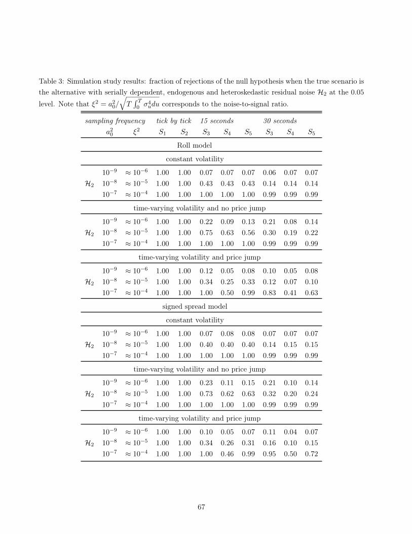
Table 3: Simulation study results: fraction of rejections of the null hypothesis when the true scenario isthe alternative with serially dependent, endogenous and heteroskedastic residual noise H2 at the 0.05

level. Note that ξ2 = a20/√T∫ T

0 σ4udu corresponds to the noise-to-signal ratio.

sampling frequency tick by tick 15 seconds 30 secondsa2

0 ξ2 S1 S2 S3 S4 S5 S3 S4 S5

Roll model

constant volatility

10−9 ≈ 10−6 1.00 1.00 0.07 0.07 0.07 0.06 0.07 0.07H2 10−8 ≈ 10−5 1.00 1.00 0.43 0.43 0.43 0.14 0.14 0.14

10−7 ≈ 10−4 1.00 1.00 1.00 1.00 1.00 0.99 0.99 0.99

time-varying volatility and no price jump

10−9 ≈ 10−6 1.00 1.00 0.22 0.09 0.13 0.21 0.08 0.14H2 10−8 ≈ 10−5 1.00 1.00 0.75 0.63 0.56 0.30 0.19 0.22

10−7 ≈ 10−4 1.00 1.00 1.00 1.00 1.00 0.99 0.99 0.99

time-varying volatility and price jump

10−9 ≈ 10−6 1.00 1.00 0.12 0.05 0.08 0.10 0.05 0.08H2 10−8 ≈ 10−5 1.00 1.00 0.34 0.25 0.33 0.12 0.07 0.10

10−7 ≈ 10−4 1.00 1.00 1.00 0.50 0.99 0.83 0.41 0.63

signed spread model

constant volatility

10−9 ≈ 10−6 1.00 1.00 0.07 0.08 0.08 0.07 0.07 0.07H2 10−8 ≈ 10−5 1.00 1.00 0.40 0.40 0.40 0.14 0.15 0.15

10−7 ≈ 10−4 1.00 1.00 1.00 1.00 1.00 0.99 0.99 0.99

time-varying volatility and no price jump

10−9 ≈ 10−6 1.00 1.00 0.23 0.11 0.15 0.21 0.10 0.14H2 10−8 ≈ 10−5 1.00 1.00 0.73 0.62 0.63 0.32 0.20 0.24

10−7 ≈ 10−4 1.00 1.00 1.00 1.00 1.00 0.99 0.99 0.99

time-varying volatility and price jump

10−9 ≈ 10−6 1.00 1.00 0.10 0.05 0.07 0.11 0.04 0.07H2 10−8 ≈ 10−5 1.00 1.00 0.34 0.26 0.31 0.16 0.10 0.15

10−7 ≈ 10−4 1.00 1.00 1.00 0.46 0.99 0.95 0.50 0.72

67

Table 4: Simulation study results: comparison of eight volatility estimators. Note that ξ2 =

a20/√T∫ T

0 σ4udu corresponds to the noise-to-signal ratio.

a20 0 10−9 mix

ξ2 0 ≈ 10−6 mix

Estimator Mean Stdv. RMSE Mean Stdv. RMSE Mean Stdv. RMSE

time-varying volatility and no price jump, tick by tick

Roll model

S 1.71e−7 3.89e−6 3.89e−6 1.33e−7 6.30e−6 6.30e−6 1.52e−7 5.24e−6 5.24e−6

QMLEexp −5.65e−8 3.10e−6 3.10e−6 4.67e−5 3.48e−6 4.68e−5 2.38e−5 2.31e−5 3.32e−5

QMLEerr 7.60e−8 5.93e−6 5.93e−6 1.02e−7 6.12e−6 6.12e−6 8.90e−8 6.03e−6 6.03e−6

EQMLE 7.61e−8 5.93e−6 5.93e−6 1.04e−7 6.12e−6 6.12e−6 8.91e−8 6.03e−6 6.03e−6

QMLE 6.13e−5 1.50e−5 6.31e−5 5.76e−5 1.53e−5 5.96e−5 5.94e−5 1.55e−5 6.14e−5

PAE −2.88e−6 2.99e−5 3.00e−5 −2.88e−6 2.99e−5 3.00e−5 −2.88e−6 2.99e−5 3.00e−5

RK 6.10e−5 1.40e−5 6.25e−5 5.86e−5 1.46e−5 6.04e−5 5.98e−5 1.39e−5 6.14e−5

RV 3.27e−4 5.87e−6 3.27e−4 3.74e−4 6.48e−6 3.74e−4 3.51e−4 6.33e−6 3.51e−4

spread model

S 1.71e−7 3.89e−6 3.89e−6 1.33e−7 6.30e−6 6.30e−6 1.52e−7 5.24e−6 5.24e−6

QMLEexp −5.66e−8 3.11e−6 3.11e−6 4.67e−5 3.48e−6 4.68e−5 2.38e−5 2.31e−5 3.32e−5

QMLEerr 7.62e−8 5.93e−6 5.93e−6 1.02e−7 6.12e−6 6.12e−6 8.91e−8 6.03e−6 6.03e−6

EQMLE 7.62e−8 5.93e−6 5.93e−6 1.04e−7 6.11e−6 6.11e−6 8.92e−8 6.03e−6 6.03e−6

QMLE 6.15e−5 1.51e−5 6.33e−5 5.78e−5 1.53e−5 5.98e−5 5.96e−5 1.56e−5 6.16e−5

PAE −2.87e−6 2.99e−5 3.00e−5 −2.87e−6 2.99e−5 3.00e−5 −2.87e−6 2.99e−5 3.00e−5

RK 6.11e−5 1.41e−5 6.27e−5 5.88e−5 1.47e−5 6.06e−5 6.00e−5 1.44e−5 6.17e−5

RV 3.31e−4 5.95e−6 3.31e−4 3.78e−4 6.51e−6 3.78e−4 3.55e−4 6.38e−6 3.55e−4

68

Table 5: Descriptive statistics

Name Ticker Nb. Trades Price Tick Price/Tick Spread(daily) (×10−3) (in ticks)

Accor ACCP 1,900 31.87 0.005 6.37 3.04Air Liquide AIRP 4,116 94.64 0.01 9.46 2.53Alstom ALSO 2,818 42.55 0.005 8.51 2.75Alcatel ALUA 3,667 4.13 0.001 4.13 1.52AXA AXAF 3,156 15.03 0.005 3.01 1.25Bouygues BOUY 2,275 34.13 0.005 6.83 1.80Credit Agricole CAGR 3,014 11.74 0.005 2.35 1.17Cap Gemini CAPP 2,002 40.83 0.005 8.17 2.04Danone DANO 3,525 46.30 0.005 9.26 2.07Airbus EAD 1,589 20.95 0.005 4.19 2.01Essilor International ESSI 1,090 52.80 0.01 5.28 2.43France Telecom FTE 2,327 15.76 0.005 3.16 1.16Engie GSZ 3,513 28.26 0.005 5.65 1.68Lafarge LAFP 3,344 44.36 0.005 8.87 3.58Louis Vuitton LVMH 2,073 112.51 0.05 2.25 1.15L’Oreal OREP 2,582 82.99 0.01 8.30 2.55Peugeot PEUP 2,129 28.17 0.005 5.63 2.77Kering PRTP 961 109.15 0.05 2.18 1.22Publicis Groupe PUBP 2,412 40.14 0.005 8.03 1.98Renault RENA 3,728 39.43 0.005 7.89 2.78Sanofi SASY 3,622 50.14 0.01 5.01 1.35Schneider Electric SCHN 2,638 121.66 0.05 2.43 1.15Suez SEVI 1,115 14.52 0.005 2.90 1.57Vinci SGEF 3,133 44.44 0.005 8.89 2.76Societe Generale SOGN 6,710 46.40 0.005 9.28 3.14STMicroelectronics STM 2,921 8.72 0.001 8.72 3.15Technip TECF 3,192 75.78 0.01 7.58 2.13Total TOTF 5,909 43.09 0.005 8.62 1.80Unibail Rodamco UNBP 1,440 153.95 0.05 3.08 1.28Veolia Environnement VIE 1,724 21.97 0.005 4.39 1.51Vivendi VIV 2,710 20.35 0.005 4.07 1.26

69

Table 6: Measure of goodness of fit of several leading models†

Model for the MMN residual noise Proportion ofexplicative part variance variance variance explained

sampling frequency: tick by tick

null 1.63× 10−8 1.63× 10−8 0.00 %Roll 2.27× 10−8 3.89× 10−9 83.84 %Glosten-Harris 2.28× 10−8 3.40× 10−9 85.97 %signed timestamp 1.82× 10−8 1.45× 10−8 20.98 %signed spread 2.78× 10−8 2.45× 10−10 99.19 %signed quote depth 2.02× 10−8 7.95× 10−9 59.71 %order flow imbalance 1.61× 10−8 1.55× 10−8 3.86 %NL signed spread 2.77× 10−8 2.44× 10−10 99.17 %general 2.79× 10−8 1.88× 10−10 99.36 %

sampling frequency ≈ 15 seconds

null 1.51× 10−8 1.51× 10−8 0.00 %Roll 2.08× 10−8 2.67× 10−9 88.67 %Glosten-Harris 2.11× 10−8 2.35× 10−9 90.09 %signed timestamp 1.58× 10−8 1.39× 10−8 15.27 %signed spread 2.61× 10−8 2.84× 10−10 99.04 %signed quote depth 1.87× 10−8 7.02× 10−9 64.68 %order flow imbalance 1.50× 10−8 1.44× 10−8 4.11 %NL signed spread 2.61× 10−8 2.84× 10−10 99.04 %general 2.63× 10−8 2.13× 10−10 99.22 %

sampling frequency ≈ 30 seconds

null 1.24× 10−8 1.24× 10−8 0.00 %Roll 1.98× 10−8 3.87× 10−9 92.17 %Glosten-Harris 2.03× 10−8 1.63× 10−9 93.34 %signed timestamp 1.33× 10−8 1.20× 10−8 21.80 %signed spread 2.46× 10−8 3.99× 10−10 98.01 %signed quote depth 1.71× 10−8 5.66× 10−9 71.77 %order flow imbalance 1.19× 10−8 1.12× 10−8 5.63 %NL signed spread 2.45× 10−8 3.98× 10−10 98.00 %general 2.47× 10−8 3.75× 10−10 98.41 %

†The MMN variance, the residual noise variance and the proportion of variance explained are estimated using πV and averagedacross the thirty one constituents of the CAC 40 and the 19 days in April 2011.

70

Table 7: Fraction of rejections of the null hypothesis at the 0.05 level for the signed spread model†

Ticker Est. Par. Var. Ex. Aver. S1 S2

Sampling frequency: tick by tick

ACCP 0.84 99.78 % 0.00 0.00 0.00AIRP 0.79 100.00 % 0.00 0.00 0.00ALSO 0.84 99.69 % 0.00 0.00 0.00ALUA 0.82 100.00 % 0.05 0.05 0.05AXAF 0.73 99.63 % 0.00 0.00 0.00BOUY 0.79 100.00 % 0.05 0.05 0.05CAGR 0.74 99.70 % 0.05 0.05 0.05CAPP 0.85 100.00 % 0.11 0.11 0.11DANO 0.82 100.00 % 0.11 0.11 0.11EAD 0.81 99.96 % 0.03 0.00 0.05ESSI 0.82 99.89 % 0.00 0.00 0.00FTE 0.74 93.92 % 0.16 0.16 0.16GSZ 0.80 99.56 % 0.00 0.00 0.00LAFP 0.82 100.00 % 0.00 0.00 0.00LVMH 0.72 94.45 % 0.11 0.11 0.11OREP 0.80 99.90 % 0.03 0.00 0.05PEUP 0.84 99.48 % 0.00 0.00 0.00PRTP 0.72 98.61 % 0.00 0.00 0.00PUBP 0.82 100.00 % 0.00 0.00 0.00RENA 0.85 99.89 % 0.00 0.00 0.00SASY 0.75 99.72 % 0.00 0.00 0.00SCHN 0.68 92.47 % 0.42 0.42 0.42SEVI 0.75 99.97 % 0.00 0.00 0.00SGEF 0.85 99.75 % 0.00 0.00 0.00SOGN 0.87 99.87 % 0.00 0.00 0.00STM 0.87 100.00 % 0.00 0.00 0.00TECF 0.75 99.99 % 0.05 0.05 0.05TOTF 0.78 100.00 % 0.00 0.00 0.00UNBP 0.69 99.23 % 0.00 0.00 0.00VIE 0.77 99.95 % 0.00 0.00 0.00VIV 0.72 99.63 % 0.00 0.00 0.00

Average 0.79 99.19 % 0.06 0.06 0.06†The values are averaged across the 19 days in April 2011. The column "Est. Par." stands for the estimated parameter and "Var.Ex." for "Proportion of variance explained". The column "Aver." corresponds to the fraction of rejections averaged across the two

tests computed using tick by tick data.

71

Table 8: Fraction of rejections for the estimated efficient price related to the signed spread model atthe 0.05 level†

Price Aver. H1 H2 H3 T AC H4

Main group

Est. price 0.06 0.08 0.05 0.05 0.05 0.09 0.04

Minor group

Est. price 0.38 0.42 0.35 0.39 0.39 0.39 0.33

Overall

Est. price 0.09 0.11 0.07 0.08 0.08 0.12 0.07Mid price 0.25 0.31 0.21 0.25 0.25 0.29 0.19Obs. price 1.00 1.00 1.00 1.00 1.00 1.00 0.99

/

†The values are averaged across the 19 days in April 2011. The column "Aver." corresponds to the fraction of rejections averagedacross the six tests. The six tests from [Aït-Sahalia and Xiu, 2016] are implemented at the tick by tick frequency considering theestimated efficient price as the given observed price to be tested. We report the proportion of rejections for each constituent when

considering the estimated price. We also report in "Obs. price" (respectively "Mid price") the proportion of rejections whenconsidering the observed price (resp. the mid price). Finally, note that the main group corresponds to stocks a priori free of

residual noise given our implemented tests, whereas the minor group stands for stocks with residual noise.

72

Figure 1: An example of estimated efficient price related to the signed spread model.

73

Figure 2: First lag of the autocorrelation function over time related to the estimated efficient pricewith the signed spread model (above) and the observed price (below) for the across-the-assets averageand 4 random assets.

74

Figure 3: Average daily signature plot for the CAC 40 constituents. Seven volatility estimators areimplemented: RV, QMLE, PAE, RK, MRK (i.e. a modified realized kernel-based estimator robust toautocorrelated-noise considered in [Varneskov, 2017]), TSRV and RV on the estimated efficient pricerelated to the signed spread model.

75

Figure 4: Estimated parameter related to the signed spread model over time average across the CAC40 constituents.

76