TESTING FEASIBILITY OF INDUCTIVE POWER COUPLING FOR MODERN APPLICATIONS

by

Andrew Burman

BioResource and Agricultural Engineering

BioResource and Agricultural Engineering Department

California Polytechnic State University

San Luis Obispo

2016

ii

TITLE : Testing Feasibility of Inductive Power Coupling for Modern Applications

AUTHOR : Andrew Burman

DATE SUBMITTED : June 3, 2016

Art MacCarley Senior Project Advisor Signature Date Charlie Crabb Department Head Signature Date

iii

ABSTRACT

This project takes two bifilar tesla coils and uses them to find a % efficiency of power transfer as distances between the coils decrease. The reason this experiment is being conducted is to find possible implications for wireless charging of vehicles using similar style coils. This project conducted experiments on 60 Hz, 400 Hz, and 1 kHz frequencies for a small input signal. The general conclusion is that as the frequency increases more power can be transferred and higher efficiency of power transfer is seen. This project also concluded that it could be possible to get higher efficiency at a greater distance with a higher input power frequency. There would of course be tradeoffs for achieving a certain charge time, but this project is concerned in the possibility of a greater gap being used so that charging could be done on a wide variety of vehicle applications. These applications would range from public transport, domestic, or freight.

iv

DISCLAIMER STATEMENT

The university makes it clear that the information forwarded herewith is a project resulting from a class assignment and has been graded and accepted only as a fulfillment of a course requirement. Acceptance by the university does not imply technical accuracy or reliability. Any use of the information in this report is made by the user(s) at his/her own risk, which may include catastrophic failure of the device or infringement of patent or copyright laws.

Therefore, the recipient and/or user of the information contained in this report agrees to indemnify, defend and save harmless the State its officers, agents and employees from any and all claims and losses accruing or resulting to any person, firm, or corporation who may be injured or damages as a result of the use of this report.

v

TABLE OF CONTENTS

SIGNATURE PAGE . . . . . . . . . . . . . . . . . . . . . . . . . . . . . . . . . . . . . . . . . . . . . . . ii

ABSTRACT . . . . . . . . . . . . . . . . . . . . . . . . . . . . . . . . . . . . . . . . . . . . . . . . . . . . . iii

DISCLAIMER STATEMENT . . . . . . . . . . . . . . . . . . . . . . . . . . . . . . . . . . . . . . . . iv

LIST OF FIGURES . . . . . . . . . . . . . . . . . . . . . . . . . . . . . . . . . . . . . . . . . . . . . . . vi

LIST OF TABLES . . . . . . . . . . . . . . . . . . . . . . . . . . . . . . . . . . . . . . . . . . . . . . . . viii

INTRODUCTION . . . . . . . . . . . . . . . . . . . . . . . . . . . . . . . . . . . . . . . . . . . . . . . . . . 1

LITERATURE REVIEW . . . . . . . . . . . . . . . . . . . . . . . . . . . . . . . . . . . . . . . . . . . . . 3

PROCEDURES AND METHODS . . . . . . . . . . . . . . . . . . . . . . . . . . . . . . . . . . . . . 9

Design Procedure . . . . . . . . . . . . . . . . . . . . . . . . . . . . . . . . . . . . . . . . . . . 9

Testing Procedure . . . . . . . . . . . . . . . . . . . . . . . . . . . . . . . . . . . . . . . . . . , 18

RESULTS AND DISCUSSION. . . . . . . . . . . . . . . . . . . . . . . . . . . . . . . . . . . . . . . 21

RECOMMENDATIONS . . . . . . . . . . . . . . . . . . . . . . . . . . . . . . . . . . . . . . . . . . . . 24

REFERENCES . . . . . . . . . . . . . . . . . . . . . . . . . . . . . . . . . . . . . . . . . . . . . . . . . . 25

APPENDICES . . . . . . . . . . . . . . . . . . . . . . . . . . . . . . . . . . . . . . . . . . . . . . . . . . . 27

Appendix A: How Project Meets Requirements for The BRAE Major . . . . 28

Appendix B: Experiment Circuit Schematic . . . . . . . . . . . . . . . . . . . . . . . 32

Appendix C: Calculations . . . . . . . . . . . . . . . . . . . . . . . . . . . . . . . . . . . . . 34

Appendix D: Data Tables . . . . . . . . . . . . . . . . . . . . . . . . . . . . . . . . . . . . . 36

Appendix E: Graphs of Data . . . . . . . . . . . . . . . . . . . . . . . . . . . . . . . . . . . 40

vi

LIST OF FIGURES

1. Example of The Right-hand Rule . . . . . . . . . . . . . . . . . . . . . . . . . . . . . . . . . . . 4

2. Example of a transformer with a primary and secondary coil . . . . . . . . . . . . . 4

3. Depiction of a Bifilar Coil. Patented by Nikola Tesla . . . . . . . . . . . . . . . . . . . . 6

4. Dynamic charging system for a car and length of road . . . . . . . . . . . . . . . . . . 7

5. Proposed circuit for the Primary coil as roadway circuit, and secondary coil as car charging circuit . . . . . . . . . . . . . . . . . . . . . . . . . . . . . . . . . . . . . . . . . . . . . . . . 8

6. Equipment for making the coils with callouts . . . . . . . . . . . . . . . . . . . . . . . . . . 9

7. Acrylic 12"x12"x0.220" sheets used as coil design kit . . . . . . . . . . . . . . . . . . 10

8. Acrylic assembled with ½”-13 threaded bolt, ½”-13 nut, and washer as a spacer . . . . . . . . . . . . . . . . . . . . . . . . . . . . . . . . . . . . . . . . . . . . . . . . . . . . . . . . 11

9. 20 AWG copper wire inserted to bottom acrylic piece and fixed with tape . . 12

10. Close up of the first few turns of a coil . . . . . . . . . . . . . . . . . . . . . . . . . . . . . 13

11. Finished coil with first application of epoxy . . . . . . . . . . . . . . . . . . . . . . . . . 14

12. Finished coil affixed with tape for next application of epoxy . . . . . . . . . . . . 15

13. Lexan mounted to 12”x6”x2” wood planks . . . . . . . . . . . . . . . . . . . . . . . . . . 15

14. Equipment for Experimentation Procedure with callouts . . . . . . . . . . . . . . 16

15. Experimentation setup of coils mounted to Lexan sheets and wood base . 17

16. Experiment with circuits attached, oscilloscope cable, function generator cable, and measurement equipment to keep the bases straight . . . . . . . . . . . . 18

17. Simplified testing setup showing the wood and Lexan base for the coils . . 19

18. Experiment Circuit Schematic . . . . . . . . . . . . . . . . . . . . . . . . . . . . . . . . . . . 33

19. Graphical data for 60 Hz Measured Output Voltage vs. Distance . . . . . . . . 39

20. Graphical data for 400 Hz Measured Output Voltage vs. Distance . . . . . . . 40

21. Graphical data for 1 kHz Measured Output Voltage vs. Distance . . . . . . . . 41

vii

22. Combined graphical data for 60 Hz, 400 Hz, and 1 kHz Measured Output Voltage vs. Distance . . . . . . . . . . . . . . . . . . . . . . . . . . . . . . . . . . . . . . . . . . . . . 42

23. Graphical data for 60 Hz Calculated Output Power vs. Distance . . . . . . . . 43

24. Graphical data for 400 Hz Calculated Output Power vs. Distance . . . . . . . 44

25. Graphical data for 1 kHz Calculated Output Power vs. Distance . . . . . . . . 45

26. Combined graphical data for 60 Hz, 400 Hz, and 1 kHz Calculated Output Power vs. Distance . . . . . . . . . . . . . . . . . . . . . . . . . . . . . . . . . . . . . . . . . . . . . . 46

viii

LIST OF TABLES

1. 60 Hz Experimental Data . . . . . . . . . . . . . . . . . . . . . . . . . . . . . . . . . . . . . . . . 35

2. 400 Hz Experimental Data . . . . . . . . . . . . . . . . . . . . . . . . . . . . . . . . . . . . . . . 36

3. 1 kHz Experimental Data . . . . . . . . . . . . . . . . . . . . . . . . . . . . . . . . . . . . . . . . 37

1

INTRODUCTION

Wireless power was first discovered by a man named Nikola Tesla, one of the

brightest, yet possibly most insane inventors of the 19th century. From his

Colorado Springs weather experiments to the AC Motor, he has impacted the

world so much as to give us a basis for power transfer that superseded that of

Thomas Edison. Unfortunately, he died before any of his larger, more intriguing

experiments could come to fruition, such as his large scale Tesla Coils for

widespread power transfer. Yet still his ideas have been implemented in ways

even he couldn’t have imagined like Wi-Fi systems that enjoyed at local

Starbucks’. One true travesty of his early demise is that he never was able to see

the abuse of the motor industry that utilizes his AC motor and its stagnation for

experimentation and technological improvement. Tesla’s design for the AC motor

was created in the late 19th century, and the US Department of Transportation

reports that the MPG for the average car in 2015 is only six MPG greater than

cars created in 2005. This a shockingly small change for such a long period of

time, most likely caused by ties drawn between oil and car companies creating a

system where they benefit from each other’s lack of technological advancements.

Electric vehicles have been around since the 1980s yet Tesla, the car company,

has just begun to become a house-hold name after decades of the idea being

around.

No, electric cars will not correct the effects of global warming and greenhouse

gas emissions, but it’s a baby step in the right direction towards a brighter,

smarter future. Integrating electric vehicles into systems that do not utilize fossil

fuels for their power source is something that is not backed by the US

Government as much as it is in other countries. Korea, for example, has the

Office for Low Emission Vehicles (OLEV) busses that use resonant inductive

charging (RIC) to charge the bus at bus stops. It uses a battery with a rather

short supply, but since it gets frequent, short charges, it is able to stay charged to

run the whole day with zero emissions. Thankfully, there are some bright minds

in the California legislature who passed the Green Schools Initiative launching

California as the nation-wide leader of solar power for schools. The Solar

Foundation states that nearly 1000 schools in 2012 had installed solar panels on

their school roofs and over their parking lots, creating a capacity of 218 kW.

While this is an amazing step for creating widespread availability of natural

energy, there is still more that can be done by integrating systems like RIC into

the parking spaces and creating an intuitive, easy way to charge vehicles without

2

the concern of the consumer. At local stores (e.g. Walmart, Target, etc...) there

has been an increase in parking spaces designated for electric vehicles complete

with a charging station. This is a positive initiative but there are problems with

direct connection chargers. People could steal the copper contacts, vandalize the

hosing and charge bay, weather conditions (rain and humidity) could degrade the

contacts, and uninformed persons could misuse or damage either the charger or

their car charge port. This is why there is a need for an RIC system that could get

rid of these issues. Taking the method from the OLEV bus, having a charge bay

underneath a parking space would allow the consumer to simply park their car

and go on with their day as it charges. They would be unaware of the charging

and for most cases (suburban living and general transportation) would not need

to worry about their battery life.

RIC is a complicated task to tackle, so this project will take the basis of the idea

and attempt to find a convention for using different types of inductors and see if

they could have a place in modern day designs for wireless power charging.

Perhaps the largest issue at hand is that as distances increase between primary

and secondary coils, the efficiency of the power transfer worsens. This project

will take the bifilar coil and determine possible uses and efficiency ranges for a

variety of distances. Since this project’s main focus will be for future use this

project will assess the capabilities of the coils with varying frequency over varying

distance. This will be done by applying an input signal via a signal generator and

amplifying the signal with an operational amplifier. The output voltage will be

recorded as the distance decreases to see the effects of frequency on the

declining distance. With this data recorded a %efficiency can be found and used

to make conclusions about usable ranges and possible future applications.

3

LITERATURE REVIEW

Background. During a class experiment in 1819, Hans Christian Oersted

accidently discovered the magnetic field by having a compass near a charged

circuit, effectively giving birth to the study of electromagnetism. (Knight 2007)

Taking Oersted’s discovery, Michael Faraday discovered the laws of

electromagnetic induction in 1831 when turning electromagnets on and off on a

closed loop circuit. (Knight 2007) Faraday’s law states that a time-varying flux

causes an induced electromotive force, or emf. (Rizzoni 2005) The magnitude of

an emf, epsilon (ε), is shown below in Equation 1:

𝜀 = 𝑁 |𝑑𝛷𝑝𝑒𝑟 𝑐𝑜𝑖𝑙

𝑑𝑡| = 𝑁|

𝑑𝐴𝐵

𝑑𝑡| (1)

This equation defines phi (Φ) as the magnetic flux that is equal to A*B, where A

is the area of the loop, and B is the magnetic field. Dividing the emf by the

resistance in the circuit will solve for the induced current, I, as shown in equation

2:

𝐼 = 𝜀

𝑅 (2)

It is important to note that there will be no emf if the voltage through an inductor

coil is constant, only when there is a change in voltage. This was discovered by

moving magnets in and out of the circuit, or in Oersted’s case, a compass flipping

sides. The readings in current meters, or from the compasses, showed that there

was a directionality with the emf.

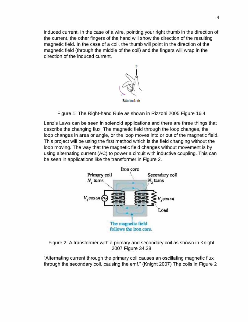
Lenz’s Law, discovered by Heinrich Lenz in 1834, creates the basis for the “right

hand rule” for the orientation of the magnetic field created. Lenz’s Law states:

“There is an induced current in a closed, conducting loop if and only if the

magnetic flux through the loop is changing. The direction of the induced current

is such that the induced magnetic field opposes the change in the flux.” (Knight

2007) Figure 1 shows an example of the right-hand-rule and how it can

determine the direction of the resultant magnetic field based on the direction of

4

induced current. In the case of a wire, pointing your right thumb in the direction of

the current, the other fingers of the hand will show the direction of the resulting

magnetic field. In the case of a coil, the thumb will point in the direction of the

magnetic field (through the middle of the coil) and the fingers will wrap in the

direction of the induced current.

Figure 1: The Right-hand Rule as shown in Rizzoni 2005 Figure 16.4

Lenz’s Laws can be seen in solenoid applications and there are three things that

describe the changing flux: The magnetic field through the loop changes, the

loop changes in area or angle, or the loop moves into or out of the magnetic field.

This project will be using the first method which is the field changing without the

loop moving. The way that the magnetic field changes without movement is by

using alternating current (AC) to power a circuit with inductive coupling. This can

be seen in applications like the transformer in Figure 2.

Figure 2: A transformer with a primary and secondary coil as shown in Knight 2007 Figure 34.38

“Alternating current through the primary coil causes an oscillating magnetic flux

through the secondary coil, causing the emf.” (Knight 2007) The coils in Figure 2

5

are wrapped around a conductive iron core undergoing alternating induced

currents to generate electromotive forces. This ultimately gives birth to

alternating current as a form of power for the entire world, later proposed by

Nikola Tesla in the late 1800s. By using different frequencies, the alternating

current reverses the magnetic field a number of times per second, which is very

similar to how Faraday and Oerstad first discovered emf by switching the

direction of a magnet or turning off the induced current to a circuit. Examples of

the utilities of a transformer are powerlines that use 60 Hz frequency for North

and South America. Other applications include radio, television, and

telecommunication services that use frequencies ranging 10^2 to 10^9 Hz.

(Knight 2007) The primary and secondary coils of Figure 2 determines the ratio

of voltage transfer in the system as seen in equation 3:

𝑉2 = 𝑁2

𝑁1𝑉1 (3)

A step-up transformer, with N2 >> N1 boosts the voltage of a generator allowing

for better transportation of energy through powerlines. The more common seen

transformers are those used in urban areas, called step-down transformers,

where N1 >> N2, so that the voltage can be lowered for house-hold appliances.

(Knight 2007)

In order to calculate the efficiency of the power transfer across the primary and

secondary coils, the power of each needs to be calculated. Knight (2007) defines

power as the rate of energy transfer in equation 4:

𝑃 = 𝐼𝑉 (4)

Taking the power calculated across the primary and secondary coils (to be

further defined as P1 for primary and P2 for secondary), setting them equal to

each other and then dividing P2 by P1 to find the efficiency of the power transfer

as seen in equation 5:

𝐸𝑓𝑓𝑖𝑐𝑖𝑒𝑛𝑐𝑦 =𝑃2

𝑃1 (5)

6

Bifilar Coil. This project will utilize two Bifilar coils (flat wound copper coil) (Figure

3)

The Bifilar coil, commonly known as the Pancake Tesla Coil, was patented by

Nikola Tesla in 1894. It takes the traditional longitudinal wound copper wire,

stacks it on itself, and makes a flat, pancake-like shape. The bifilar coil can have

one wire wrapped tightly together, or it could have two wires bound together, and

may have shielded wires to reduce the amount of power losses at higher

frequency usage.

Types of power losses for these inductors include eddy currents and skin effects.

“[Eddy currents is the] dissipation of energy into heat” inside of the core (Rizzoni

2005). As the magnetic flux affects the core the conductor will heat up and there

will be a direct loss of energy in the form of heat. This makes the ferrite core

impractical in situations without good ventilation or in smaller applications where

heat could cause malfunctions of a device. Instead, by using an air core, there

will be less losses for some of its applications, but not all. Known as skin effect,

there are losses in an air core that is based on the cross sectional area of the

wire used for the coil. “With a round wire this causes the current density to be

maximum at the surface and least at the center” (Terman 1943). This is why

several types of air cores can be found on the market utilizing rectangular wire

designs. By flattening the wire used, it increases the outer surface area, which in

turn, reduces the amount of inner material that will not carry as much current.

Essentially, when more material is carrying more current (when flattened or

elongated), the higher the inductance and lower the resistance (Terman 1943).

Current Technologies. There are several types of systems for dynamic charging

of electric vehicles, such as the OLEV bus in Korea (Jeong el. al. 2015) and also

Figure 3. Depiction of a Bifilar Coil. Patented by Nikola Tesla. Tesla, N. 1894 Figure 2.

7

the inductive power transfer highway. (Russer et. al. 2014) These systems utilize

an isolated long track of primary coil that is underground and secondary coils

inside the moving vehicle. (Wang et. al. 2005) Figure 4 shows a simplified

version of how it works, where the primary coil could run along a length of

highway, utilizing power from the grid to generate its initial magnetic field. The

secondary coil would line the underside of the car and there would be an internal

converter to switch the absorbed magnetic field into DC power to power the

electric motor.

Figure 4: Idea of a dynamic charging system for a car and length of road. Wang et. al. 2005

The issue with using this for cars is that to maximize efficiency of the circuit, the

height of the cars would need to all be the same. This puts an additional design

constraint on car makers, but also leaves way for innovation on side of the

secondary coil and internal inverter as it is up to the car maker for the optimal

way to design it. In the application of the public transport bus in Korea, the OLEV

bus was able to use smaller, lighter batteries for its power source because it was

always frequently charging in small bursts. (Jeong et. al. 2015)

Russer et. al. (2015) propose a method of magnetic-resonant wireless power

transfer (MRWPT) that could solve the current problem of inefficiency in roadway

powering of electric vehicles. Using a similar method to a parked car format for

wireless charging, the circuit that has a length of multiple loops of primary coils

that will only activate when there is full alignment with the secondary coil. This,

most likely, is to maximize efficiency, but could also minimize the amount of

wasted energy by having a constantly powered roadway system. This can be

seen in figure 5, with the load moving to the right, as it crosses from LP2 to LP3.

The switches activate when the maximum current has been reached, switching

the magnetic wave generation from one primary coil to the next. This will also

help the spread of the wave function, attempting to keep the phases as close as

8

possible to maximize current flow. (Note: Figure 7 depicts a design indicative of a

resonant inductive system, which is not what will be studied for this project.)

Figure 5: Proposed circuit for the Primary coil (bottom) as the roadway circuit connected to the power grid, and the secondary coil (top, load circuit) that feeds

into the car to charge the vehicle. Russer et. al. 2015

The relevance of this project is to see if the aforementioned inductors could be

beneficial to the OLEV and other dynamic systems. By testing the range

(efficiency and distance between coils) at which these inductor types can be

used could be transferred to larger scale applications. In order to find out which

type is more beneficial for a long range system, this project will require multiple

types to be tested. Hopefully, a conclusion can be made between the usefulness

of a certain type of inductor at longer ranges so that it can be utilized in future

applications.

9

PROCEDURE AND METHODS

Design Procedure

Design and Building of Coil Builder. In order for the coils to be wound tightly and

easily, a device was designed and built to accommodate the process. The

materials used are shown in Figure 6 and listed below.

A: 12”x12”x0.220” acrylic with four ½” slots and one ½” hole.

B: 12”x12”x0.220” acrylic with two 1/32” holes and one ½” hole.

C: Epoxy

D: Tape

E: Two 200’ spools of 20 AWG copper wire

F: One 5” long ½”-13 threaded bolt

G: Two half inch washers

H: One ½”-13 nut

Figure 6: Equipment for making the coils with callouts

10

The acrylic used can be more clearly seen in Figure 7. The top acrylic piece has

slots so that epoxy can be added once the turning of the coil has been

completed. The bottom acrylic piece has two 1/32” holes for where the wires will

be pinned down to create an anchor point for turning the coil. These holes are

drilled ¾” away from the center hole so that a washer can fit between both acrylic

pieces and act as a spacer.

The acrylic pieces will be bound together with the ½”-13 threaded bolt and nut

with the spacer in between as shown in Figure 8. Also shown in Figure 8 are two

1/32” holes just outside of the diameter of the washer allowing for room for the

copper wire and will act as anchor points during the turning of the coil.

Figure 7: Acrylic 12"x12"x0.220". The right piece is to act as a top and is slotted for accessibility to the wire to put on epoxy or fix layout of wire. The left piece is

to act as a bottom that fits the copper wire.

11

With a form developed for how to turn the coils efficiently, the building of the coils

can begin.

Turning the Coils. The spools of copper wire are inserted into the small holes of

the bottom acrylic piece then being affixed to the bottom of the acrylic with tape.

It is important to remember which wire end is from which spool because two

need to be soldered together, while two will be used as a positive and negative

end of the coil. This initial setup is shown below in Figure 9.

Figure 8: Acrylic assembled with ½”-13 threaded bolt, ½”-13 nut, and washer as a spacer. (A) and (B) from Figure 1 are used as a top and bottom piece

respectively.

12

For the finished coil, either (A) and (C), or (B) and (D) need to be soldered

together, therefore it is important to pay careful attention to how this setup is

done as to not confuse which wires will be soldered and which will be left alone.

This can be done by keeping the positions of the spools constant, and turning the

acrylic, counting the amount of turn based off of the initial contact area of the two

wires. The way it is setup in Figure 9, that turn count position also correlates to

one of the slots of the top acrylic piece.

With the wires in place, the bolt is then slotted, the washer put around it, then the

acrylic pieces can be tightened together. The nut should be tightened until the

acrylic pieces cannot shift positions. Keeping the wire taught, turn the acrylic and

begin turning the coil. Figure 10 shows the first few turns of a coil.

Figure 9: 20 AWG copper wire inserted to bottom acrylic piece and fixed with tape.

A

B

C

D

13

As the number of turns increases it can be hard to keep the wire organized, but

the slots on the top acrylic allow for some maintenance. However, if the wire is

too thin it may be difficult to maintain tidiness. It is more important to keep the

wire tight so that it does not loosen and cause gaps in the finished coil and also

to ensure it does not unwind when loosening the bolt and taking the contraption

apart.

For this project two coils were made: One with 80 turns and the other with 120

turns. This was done to create a turn ratio of 2:3. This was done to mimic what

would most likely be a future setup for future applications by using a step up

system.

When the desired amount of turns has been reached, the slots in the top acrylic

provide a space for epoxy to be added as seen in Figure 11. Before removing the

coil and cutting it free from the copper spools, a length of about 2 feet of wire was

left loose for use in circuitry and soldering later on.

Figure 10: Close up of the first few turns of a coil.

14

After the first set of epoxy has hardened, the coil can be removed and will keep

reasonably tight. It can then be flipped over and epoxied on the opposite side, or

taped and epoxied in higher quantity outside of the acrylic contraption. Figure 12

shows one of the finished coils made for this project. It was removed before

being fully epoxied on the backside so that it could be epoxied to a piece of

Lexan as flat as possible. The Lexan is used for the experimental procedure

discussed further in the next section.

Figure 11: Finished coil with first application of epoxy

15

Experimentation Equipment. The main experimental hardware consists of two

8”x6”x2” pieces of wood, and two 12”x12”x0.093” pieces of Lexan. Two holes

were drilled into each piece: a 3/8” hole and a ½” hole. Each piece of Lexan was

attached to a piece of wood so that it could stand freely, as seen in Figure 13.

Figure 12: Finished coil affixed with tape for next application of epoxy

Figure 13: Lexan mounted to 12”x6”x2” wood planks

16

Experimentation equipment for coil bases as seen in Figure 14:

A: One 12” long ½”-13 brass threaded rod

B: Three ½” brass washers

C: Three ½”-13 brass nuts

D: 741 operational amplifier

E: 1.5 Ohm resistor (Dale CW-2C Wire wound resistor)

F: 100k Ohm resistor

The coils epoxied to the Lexan and the copper wires trimmed and soldered

accordingly as seen in Figure 15. The wires that were initially used as anchors

for turning will go through the center hole of the Lexan. A hole closer to the

bottom of the piece – located near the wood base – will act as the location for the

brass rod to bind both mounted coils together. This brass rod, accompanied with

the brass washers and nuts, will help keep the coils lined up and tightening the

nuts will draw the coils closer together to gather experimental data.

The load resistor is a 1.5 Ohm wire-wound resistor which is more capable of

dealing with higher temperatures and current than the average resistor. The 100k

ohm resistor is used as the grounding resistor in the open loop operational

amplifier circuit to increase the gain as much as possible to increase the input

signal of the function generator.

Figure 14: Equipment for Experimentation Procedure with callouts

17

The experiment required taking the assembly in Figure 9 and adding circuits to

the front end of the primary coil and a load resistor to the secondary coil (left and

right coils respectively).

The rest of the experimentation equipment can be seen in Figure 16 which

shows the actual testing setup during the testing. Schematics for the circuit

created to gather data can be seen in Appendix C. The additional equipment was

available to students via the BRAE labs 3-e and 7 and are listed below:

One set of digital calipers

One large tri-square

Two electronic breadboards

Virtual Bench for oscilloscope and function generators

Figure 15: Experimentation setup of coils mounted to Lexan sheets and wood base

18

Due to the limited length of the function generator, oscilloscope, and coil wires,

the experiment was limited to the available desk space and proved difficult to

keep tidy while gathering experimental data. The additional metal equipment (like

the tri-square) did not seem to have any effects on the input or output signals, but

the equipment in the lab itself may have caused there to be additional levels of

noise adding some variance to the readings.

Testing Procedure

The coils, mounted to the wood and Lexan base, are connected with a ½”-13

brass rod and held together with ½”-13 nuts and washers. (Figure 16)

The virtual bench allows for an oscilloscope readout for two channels. Channel

one was also used as a voltage source. The virtual bench itself does not output

much power, so an operational amplifier was used to attempt to increase the

voltage of the signal. For most of the experimentation, the input voltage

fluctuated slightly, but overall an average value of 2.22 Volts was seen.

Figure 16: Experiment with circuits attached, oscilloscope cable, function generator cable, and

measurement equipment to keep the bases straight

19

The primary coil side had two nuts bound together on both sides of the Lexan to

try and keep the rod as straight as possible and keep the secondary coil lined up

with it.

The secondary coil just had a single nut attached that, when tightened, would

slowly bring the secondary coil closer to the primary coil, reducing the distance x

as shown in Figure 17.

The function generator, via the Virtual Bench, was used to output an analog

signal of 60, 400, and 1000 Hz. The circuits and probes were connected to the

coils and a preliminary test was performed to find a rough beginning range for the

test to begin at. This was done by using the 1 kHz function generator and moving

the coils apart from each other. 1 kHz was used because it was the most

sensitive system. When there began to be a steady increase in power to the

channel two probe that was definitely not variance due to noise, that would be

the starting point. This point was determined to be 155 mm.

At the initial starting distance the other two frequencies used: 60 and 400 Hz;

were less subjected to change as the distance decreased between the coils. The

data points at this point in the experiment were 5 mm apart until there was a

notable trend in output signal for the 60 Hz and 400 Hz frequencies. When that

trend started to form in the 60 Hz data (because it is the least sensitive), the data

points were condensed to 2 mm and then finally to 1 mm for the final few tests.

For recording the data at each data point there is a button labeled “single” that

acts as a picture of the data instead of using the rather variable “auto” setting.

Figure 17. Simplified testing setup showing the wood and Lexan base for the coils. Distance x reduced for each data point.

20

With this single, or snapshot, method, a measurement was taken every 15

seconds, for 45 seconds, at each distance and each frequency. An average

value of all three points would be used for the final data interpretation. The data

gathering process was done this way to eliminate selection bias, which is

essentially trying to record values that would make the test look better. By

recording data at exact intervals, using the “single” feature, that bias was lowered

(not necessarily eliminated) and then averaged to give a more “likely” outcome of

results.

The distance between the coils was measured with calipers and was kept

straight using a tri-square. The primary coil side was essentially fixed and used

as a reference for keeping the coils square and in line. This was done by lining

up the base of the primary coil in the corner of the tri-square, and fixing the

Lexan – and therefore the primary coil – between two tight nuts. The secondary

coil had another nut and when tightened would slowly draw the secondary coil

towards the primary coil.

Data was recorded at the following intervals:

1) 5 mm intervals from 155 mm to 70 mm for a total of 18 data points.

2) 2 mm intervals from 70 mm to 30 mm for a total of 20 data points.

3) 1 mm intervals from 30 mm to 19 mm for a total of 10 data points.

There was a total of 48 data points that were used to dictate a trend line for each

frequency used.

The measurements for the distance were taken between both ends of the mounted Lexan. The actual coils were about 14 mm closer together. The corrected distance is used in the data sheets shown in Appendix D. The measurements were taken this way because there was a bit of slack due to the weight of the coils on the Lexan which was not intended and formed after assembly. This slack caused a very slight forward bend in the Lexan sheets and both coils, making the final data points more like average distances than exact distances. Again, the bend is very slight and only impacted the final range of data points as ranges closer than 5mm could not be used because the very top of the coils would touch if moved any closer.

21

RESULTS AND DISCUSSION

Effects of Frequency. The graphs in Appendix E clearly show an indication that

the effect on voltage output is greatly increased by the higher frequency of the

input signal. These graphs also show that a power curve trend line fit nearly

perfectly into most of the data sets. Having higher frequency also seemed to

increase the range at which the power transfer would occur. The starting point

was initially chosen because the output signal began to noticeably increase at 1

kHz. The frequency in which data was recorded was changed when all three

frequencies began to show increase in output voltage readings. This could have

been misconstrued due to some issues with noise, which there clearly was upon

close inspection of the first data points for each frequency. However, another

effect increasing the frequency seemed to have was that the variance in the

signal for both input and output was decreased. With this, there also seemed to

be a decrease in the impact of noise as the testing went on. This is seen by

having a higher R2 value in the trend line developed in the output voltage graphs

of Appendix E. The same graphs also show the results getting “tighter” as the

frequency increases again representing how variance in the readouts were

decreasing with change in frequency.

With the increase in frequency, the efficiency, shown by the %eff value on the

data tables in Appendix D, increases as the distance decreases. This is an effect

that is supposed to happen in general with the coils as they are more effective

the closer they are together. The interesting part is the rate at which the increase

in output voltage occurs as the frequency increases. The implication here is that

assuming the system does not overheat, a higher frequency could be used to

increase both the distance between coils and the amount of power transferred

while still achieving ample % efficiency.

Expectations and Implications. The test was expected to show that as the coils

were nearer to each other that the power transfer would nearly be equivalent,

even at lower frequencies. However, the test showed that at 60 Hz the power

transfer was almost nonexistent. Whereas, with the 400 Hz and 1 kHz signals,

the coils started to show large increases in efficiency around 30 mm and 40 mm

respectively. (Appendix E – Figures 20 and 21) This translates to about an inch

to an inch and a half gap. The coils used were very small and the overall

assumption of this test is that the same data would carry over and be magnified

by the size of the coils. This means that as the size of the coils increase then

perhaps the distance potential could increase as well. Since larger coils would be

capable of withstanding and dissipating more heat, a larger input signal could be

22

used and perhaps even a higher frequency as well (beyond 1 kHz as used in this

experiment).

Appendix D shows the data tables for each of the performed tests. In Table D-1,

the efficiency for the test never exceeds 1%. This leads to the conclusion that for

ample power transfer, the frequency would most definitely not work with simple

wall power fed into a primary coil. In Table D-2 there starts to be increasingly

larger %efficiency jumps as the distance closes. This trend isn’t as easily seen in

the 60 Hz table or in the graphs. Still, the maximum efficiency peaks at about

27% and only for the closest value. The point of this experiment was not to prove

that efficiency is highest for the closest value, but that the point at which the rate

begins to increase could dictate possible ranges for use. So, turning to Table D-

3, the peak efficiency is around 90% at the closest position, and the previously

highest efficiency of 27% (seen in Table D-2) is realized in Table D-3 between 12

to 13mm. This is a jump of nearly 10 mm, which isn’t much, but again this test

used a very small signal, with very small coils. At least in regards to this

experiment, it seems that with increasing frequencies that range of efficiency

difference will begin to increase as well, which could possibly lead to better

results when increasing the distance between coils.

The major implication here then is that if coils roughly the diameter of the width of

a car were to be used (about 65-70 inches for sedans) then the gap between the

primary and secondary coils could be relatively large without a major decrease in

efficiency. With a very rough estimation, if the test outcome from this procedure

was simply multiplied by 10 to compare it to a larger coil, then at about a gap of

400 mm would be the beginning of the increase in efficiency for the larger coil

system. Obviously, this is a very crude estimation to make, but when the margin

for usage changes from 1 inch to 15 inches, suddenly the possibilities for use

become much larger. With a larger coil there could be more environment effects

on the coil and on the power transfer, however, as seen in this experiment, as

the frequency increases, the variance tends to lessen. (Appendix E)

Experiment Validation. Similar experiments were performed with resonant circuits

so the results are expected to be different in what they are looking for, namely

the power transfer when both coils are functioning at resonance or at matching

impedance. However, by interpreting some of the 3D graphs comparing load

impedance, distance between coil, and efficiency of wireless power transfer

(WPT), Rotaru et. al (2014) show comparable results. The results shown in their

graphical data show off a similar power curve trend that was seen in the

graphical data of this experiment. The experiments conducted by Rotaru et. al

23

(2014) were done at a much higher frequency (10 kHz) and withstanding much

higher power (2 kW). Yet, there experimental procedure seemed to be very

similar to the one conducted here but utilizing the resonant features of the coils

rather than simply the inductive capabilities. Their experiment showed that with

the resonance of their coil paired with matching impedance the power transfer

efficiency was still high even at further distances. Their experimental data shows

distances of up to 300 mm, which would not be possible with the way data was

gathered with this project’s experiment, possibly due to the size of the coil and

the lack of use of resonant circuits. However, this seems to validate the data

gathered here that the nature of the inductive capabilities of the coils used

follows a power curve trend.

24

RECOMMENDATIONS

For future testing, it would be very interesting to see if the data gathered at similar ranges in this study could be repeated with larger coils. That would hopefully mean that the conclusions made in this experiment do hold some weight and that future applications could be useful.

A change that could be made to the testing procedure is to see the effects of having several different gauges of wire – both smaller and larger.

With the increase in coil size for future testing, the frequency range of these tests could also increase. This would hopefully lead to the same conclusions made here that the efficiency range would increase as the frequency increases.

One way that this experiment could be implemented in the real world is a car-port-charger that would be placed underneath a vehicle. This would require a kit to protect the coils from any environmental or direct-physical damages. It would be an interesting experiment to see how well the coils function with a bulk of material in the way. Assumedly that material would impact (perhaps a hard plastic) the emf in a minor way, but still any impact with a large distance between coils could cause a charge time to increase quite a bit.

Another change that can be made is making a series of bifilar coils and stacking them together to see the impacts of using multiples of coils either stacked in line or offset to create different patterns. It would be assumed that by having a set of smaller coils it would act similarly to having one larger coil, but any impact that may occur due to offset or misalignment could be lowered.

25

REFERENCES

Covic, G.A., Boys, J.T., 2013. Modern Trends in Inductive Power Transfer

for Transportation Applications. IEEE JOURNAL OF EMERGING AND

SELECTED TOPICS IN POWER ELECTRONICS, VOL. 1, NO. 1,

MARCH 2013, Pg. 28-41.

Jeong, S., Jang, Y. J., Kum, D., 2015. Economic Analysis of the Dynamic

Charging Electric Vehicle. IEEE TRANSACTIONS ON POWER

ELECTRONICS, VOL. 30, NO. 11, NOVEMBER 2005, Pg. 6368-6377.

Knight, R. D., 2007. Physics for Scientists and Engineers a Strategic

Approach. 2nd ed., Pearson.

Rizzoni, G., 2005. Principles and Applications of Electrical Engineering. 5th

ed., McGraw-Hill Education.

Rotaru, M.D., Tanzania, R., Ayoob, R., Kheng, T.Y., Sykulski, J.K. 2014.

Numerical and experimental study of the effects of load and distance

variation on wireless power transfer systems using magnetically coupled

resonators. IET Sci. Meas. Technol., 2015, Vol. 9, Iss. 2, pp. 160-171, doi:

10.1049/iet-smt.2014.0175

Russer, J.A., Dionigi, M., Mongiardo, M., Costanzo, A., Russer, P., 2014.

An Inductive Power Transfer Highway System for Electric Vehicles. IEEE

CALCON2014.

Terman, F.E. 1943. Radio Engineering Handbook. McGraw-Hill Book

Company, Inc., New York and London.

Tesla, N. 1894. US Patent 512340. Coil for Electro Magnets. Patented

Jan. 9, 1894.

Valtchev, S.S., Baikova, E.N., Jorge, L.R., 2012. Electromagnetic Field as

The Wireless Transporter of Energy. FACTA UNIVERSITATIS, Elec.

Energ., Vol. 25, No. 3, December 2012, Pg. 171-181.

Wang, C.S., Stielau, O.H., Covic, G., 2005. Design Consideration for a

contactless electric vehicle battery charger. IEEE TRANSACTIONS ON

INDUSTRIAL ELECTRONICS, VOL. 52, NO. 5, OCTOBER 2005, Pg.

1307-1314.

26

Yilmaz, M., Krien, P.T., 2012. Review of Battery Charger Topologies,

Charging Power Levels, and Infrastructure for Plug-In Electric and Hybrid

Vehicles. IEEE TRANSACTIONS ON POWER ELECTRONICS, VOL. 28,

NO. 5, MAY 2012. Pg. 2151-2169.

27

APPENDICES

Appendix A: How Project Meets Requirements for The BRAE Major . . . . . . . . 28

Appendix B: Calculations . . . . . . . . . . . . . . . . . . . . . . . . . . . . . . . . . . . . . . . . . . 32

Appendix C: Experiment Testing Schematic . . . . . . . . . . . . . . . . . . . . . . . . . . . 34

Appendix D: Data Tables . . . . . . . . . . . . . . . . . . . . . . . . . . . . . . . . . . . . . . . . . . 36

Appendix E: Graphs . . . . . . . . . . . . . . . . . . . . . . . . . . . . . . . . . . . . . . . . . . . . . . 40

28

APPENDIX A: HOW PROJECT MEETS REQUIREMENTS FOR THE BRAE MAJOR

29

Major Design Experience

The BRAE senior project must incorporate a major design experience. Design is the process of devising a system, component, or process to meet specific needs. The design process typically includes fundamental elements as outlined below. This project addresses these issues as follows.

Establishment of Objectives and Criteria. Project objectives and criteria are established to meet the needs and expectations of the BioResource and Agricultural Engineering Department of Cal Poly SLO.

Synthesis and Analysis. The project required the building of an experiment to test the efficiency of an inductive power coupling system. This will incorporate common circuit calculations, analysis of efficiency of a power transfer system, and the recommendation for future applications.

Construction, Testing, and Evaluation. The inductive coupling circuit was designed, constructed, tested, and evaluated for efficiency, and optimal operational distance and frequency.

Incorporation of Applicable Engineering Standards. The project utilizes IEEE, NEC, and SAE standards for recommended practice for Inductive Coordination of Electric Supply.

30

Capstone Design Experience.

The BRAE senior project is an engineering design project based on the knowledge and skills acquired in earlier coursework (Major, Support and/or GE courses). This project incorporates knowledge/skills from these key courses:

BRAE 129 Lab Skills/Safety

BRAE 133 Engineering Graphics

ENGL 149 Technical Writing

BRAE 151 AutoCAD

BRAE 216 Fundamentals of Electricity

BRAE 328 Measurements and Computer Interfacing

EE 321/361 Electronics and Electronics Laboratory

Design Parameters and Constraints.

This project addresses a significant number of the categories of constraints listed below.

Physical. Creation of a testing apparatus for inductive power coupling.

Economic. Testing potential for wireless charging to be efficient enough for multiple applications such as: domestic, freight, and public transport, removing the need to waste time going to the pump to charge or refuel a vehicle.

Environmental. Increasing the efficient usage and quality of life for electrically driven vehicles and users will add incentives for switching to electrical vehicles for means of transportation. Using electrical vehicles rather than carbon-fuel-based vehicles will lead to positive impacts on the environment.

Sustainability. Wireless charging components will be less susceptible to erosion and weathering as their direct charging counterparts.

Manufacturability. The same technology being researched here can be used in many other smaller applications such as phone chargers or to power small devices.

Health and Safety. Depending on the frequency of the applied signal, the emf generated could have adverse effects on the human body with prolonged exposure, however the overall impact is still unknown. If the frequency is high enough, sound can lead some to discomfort. Otherwise, utilizing wireless charging instead of direct charging would assumedly be safer for the user.

31

Ethical. When the technology develops for better batteries and charging technologies, there will be a reduction in total energy used.

Social. Ease and efficiency of charging could influence more widespread usage.

Political. Promote the use of more sustainable technology in agriculture and domestic practices.

Aesthetic. Vehicles utilizing a wireless charging system would have their means of recharging hidden would could allow for designers to have more intricate exterior designs of vehicles that do not need to incorporate a port for direct charging. Wireless charging can also occur in an environment that is very dirty (ag applications) that direct charging may begin to have some difficulties being as effective.

Other- Productivity. Charging of a vehicle battery could be done while parked without the hassle or need to plug in or refuel assuming the time spent on the charging bay is long enough and efficient enough to charge a battery enough for the next length of travel.

32

APPENDIX B: CALCULATIONS

33

𝑃1 = 𝑃2 (6)

𝑃2 =𝑉2

2

𝑅2 (7)

%𝐸𝑓𝑓𝑖𝑐𝑖𝑒𝑛𝑐𝑦 =𝑃2

𝑃1∗ 100% (8)

𝑉1 ∗ 𝑁2 = 𝑉2 ∗ 𝑁1 (9)

To calculate the power input (P1) equations 7 and 9 are subbed into equation 3. Using the calculated value of P1 and the measured value of P2 %efficiency will then be calculated by using equation 8.

𝑃1 = 𝑃2

𝑃1 = 𝑉2

2

𝑅2

𝑉2 = 𝑉1 ∗ 𝑁2

𝑁1

𝑉1 = 𝐼𝑛𝑝𝑢𝑡 𝑉𝑜𝑙𝑡𝑎𝑔𝑒 = 2.22 𝑉𝑜𝑙𝑡𝑠

𝑅2 = 𝐿𝑜𝑎𝑑 𝑅𝑒𝑠𝑖𝑠𝑡𝑜𝑟 𝑅𝑒𝑠𝑖𝑠𝑡𝑎𝑛𝑐𝑒 = 1.5 𝛺

𝑁1 = 80 𝑡𝑢𝑟𝑛𝑠; 𝑁2 = 120 𝑡𝑢𝑟𝑛𝑠

𝑉2 = 𝑉1 ∗ 120

80= 𝑉1 ∗ 1.5

𝑃1 = 𝑉1

2 ∗ 1.52

1.5

𝑃1 = 𝑉12 ∗ 1.5

𝑃1 = 2.222 ∗ 1.5

𝑃1 = 7.3926 𝑊𝑎𝑡𝑡𝑠

With the input power calculated once measurements have been taken during the testing, efficiency can be calculated by using equation 5.

34

APPENDIX C: EXPERIMENT CIRCUIT SCHEMATIC

35

Figure 18. Experiment Circuit Schematic

36

APPENDIX D: DATA TABLES

37

19 5 2.22 325.00 325.00 333.00 327.67 0.33 0.07 0.97%

20 6 2.21 267.00 284.00 276.00 275.67 0.28 0.05 0.69%

21 7 2.22 219.00 226.00 222.00 222.33 0.22 0.03 0.45%

22 8 2.22 243.00 222.00 226.00 230.33 0.23 0.04 0.48%

24 10 2.22 222.00 206.00 198.00 208.67 0.21 0.03 0.39%

25 11 2.22 196.00 201.00 211.00 202.67 0.20 0.03 0.37%

26 12 2.22 171.00 176.00 188.00 178.33 0.18 0.02 0.29%

27 13 2.22 156.00 151.00 156.00 154.33 0.15 0.02 0.21%

28 14 2.22 179.00 189.00 183.00 183.67 0.18 0.02 0.30%

29 15 2.22 170.00 148.00 150.00 156.00 0.16 0.02 0.22%

30 16 2.21 178.00 174.00 170.00 174.00 0.17 0.02 0.27%

32 18 2.22 173.00 165.00 156.00 164.67 0.16 0.02 0.24%

34 20 2.22 150.00 137.00 145.00 144.00 0.14 0.01 0.19%

36 22 2.22 143.00 137.00 150.00 143.33 0.14 0.01 0.19%

38 24 2.22 151.00 151.00 148.00 150.00 0.15 0.02 0.20%

40 26 2.22 145.00 137.00 138.00 140.00 0.14 0.01 0.18%

42 28 2.22 135.00 138.00 135.00 136.00 0.14 0.01 0.17%

44 30 2.22 132.00 125.00 125.00 127.33 0.13 0.01 0.15%

46 32 2.21 105.00 114.00 119.00 112.67 0.11 0.01 0.11%

48 34 2.21 97.10 110.00 119.00 108.70 0.11 0.01 0.11%

50 36 2.22 114.00 98.80 110.00 107.60 0.11 0.01 0.10%

52 38 2.22 93.80 114.00 127.00 111.60 0.11 0.01 0.11%

54 40 2.21 105.00 125.00 119.00 116.33 0.12 0.01 0.12%

56 42 2.21 88.10 99.60 110.00 99.23 0.10 0.01 0.09%

58 44 2.21 95.50 100.00 105.00 100.17 0.10 0.01 0.09%

60 46 2.21 82.30 69.10 105.00 85.47 0.09 0.00 0.07%

62 48 2.21 68.70 75.70 75.70 73.37 0.07 0.00 0.05%

64 50 2.22 80.70 86.40 86.80 84.63 0.08 0.00 0.06%

66 52 2.22 85.20 84.00 82.70 83.97 0.08 0.00 0.06%

68 54 2.22 99.60 77.40 88.90 88.63 0.09 0.01 0.07%

70 56 2.21 87.20 100.00 106.00 97.73 0.10 0.01 0.09%

75 61 2.21 85.20 95.10 91.80 90.70 0.09 0.01 0.07%

80 66 2.21 95.50 72.40 59.30 75.73 0.08 0.00 0.05%

85 71 2.22 65.00 52.70 59.30 59.00 0.06 0.00 0.03%

90 76 2.21 93.80 70.80 62.60 75.73 0.08 0.00 0.05%

95 81 2.22 48.60 76.50 83.10 69.40 0.07 0.00 0.04%

100 86 2.21 80.70 89.70 87.20 85.87 0.09 0.00 0.07%

105 91 2.21 85.60 92.20 80.70 86.17 0.09 0.00 0.07%

110 96 2.22 94.70 96.30 93.00 94.67 0.09 0.01 0.08%

115 101 2.22 56.00 52.70 75.70 61.47 0.06 0.00 0.03%

120 106 2.22 92.20 82.30 60.90 78.47 0.08 0.00 0.06%

125 111 2.22 79.00 119.00 104.00 100.67 0.10 0.01 0.09%

130 116 2.21 52.30 67.10 49.80 56.40 0.06 0.00 0.03%

135 121 2.21 85.60 69.10 79.00 77.90 0.08 0.00 0.05%

140 126 2.22 70.80 46.10 84.80 67.23 0.07 0.00 0.04%

145 131 2.22 94.70 90.50 74.10 86.43 0.09 0.00 0.07%

150 136 2.22 90.50 77.40 56.00 74.63 0.07 0.00 0.05%

155 141 2.22 100.00 102.00 107.00 103.00 0.10 0.01 0.10%

Distance (mm)

Power

Output

(W)

AVG

Output

(V)

Input (V)Output 1

(mV)

Output 2

(mV)

Output 3

(mV)

AVG

Output

(mV)

%Eff

Table 1. 60 Hz Experimental Data

38

19 5 2.21 1730.00 1730.00 1730.00 1730.00 1.73 2.00 26.99%

20 6 2.21 1400.00 1400.00 1400.00 1400.00 1.40 1.31 17.68%

21 7 2.21 1230.00 1230.00 1230.00 1230.00 1.23 1.01 13.64%

22 8 2.21 1230.00 1220.00 1220.00 1223.33 1.22 1.00 13.50%

24 10 2.21 1050.00 1050.00 1050.00 1050.00 1.05 0.74 9.94%

25 11 2.21 988.00 988.00 988.00 988.00 0.99 0.65 8.80%

26 12 2.21 938.00 938.00 938.00 938.00 0.94 0.59 7.93%

27 13 2.21 872.00 872.00 872.00 872.00 0.87 0.51 6.86%

28 14 2.21 856.00 856.00 856.00 856.00 0.86 0.49 6.61%

29 15 2.21 815.00 815.00 807.00 812.33 0.81 0.44 5.95%

30 16 2.21 765.00 757.00 765.00 762.33 0.76 0.39 5.24%

32 18 2.21 716.00 708.00 708.00 710.67 0.71 0.34 4.55%

34 20 2.21 667.00 667.00 667.00 667.00 0.67 0.30 4.01%

36 22 2.21 626.00 626.00 617.00 623.00 0.62 0.26 3.50%

38 24 2.21 609.00 617.00 609.00 611.67 0.61 0.25 3.37%

40 26 2.21 593.00 584.00 584.00 587.00 0.59 0.23 3.11%

42 28 2.21 547.00 556.00 551.00 551.33 0.55 0.20 2.74%

44 30 2.21 519.00 519.00 514.00 517.33 0.52 0.18 2.41%

46 32 2.21 490.00 490.00 490.00 490.00 0.49 0.16 2.17%

48 34 2.21 461.00 461.00 457.00 459.67 0.46 0.14 1.91%

50 36 2.21 449.00 453.00 449.00 450.33 0.45 0.14 1.83%

52 38 2.21 436.00 440.00 440.00 438.67 0.44 0.13 1.74%

54 40 2.21 424.00 428.00 432.00 428.00 0.43 0.12 1.65%

56 42 2.21 412.00 407.00 416.00 411.67 0.41 0.11 1.53%

58 44 2.21 395.00 395.00 399.00 396.33 0.40 0.10 1.42%

60 46 2.21 383.00 379.00 383.00 381.67 0.38 0.10 1.31%

62 48 2.21 370.00 374.00 370.00 371.33 0.37 0.09 1.24%

64 50 2.21 366.00 362.00 370.00 366.00 0.37 0.09 1.21%

66 52 2.21 354.00 346.00 354.00 351.33 0.35 0.08 1.11%

68 54 2.21 333.00 333.00 329.00 331.67 0.33 0.07 0.99%

70 56 2.21 329.00 333.00 337.00 333.00 0.33 0.07 1.00%

75 61 2.21 317.00 313.00 321.00 317.00 0.32 0.07 0.91%

80 66 2.21 288.00 296.00 300.00 294.67 0.29 0.06 0.78%

85 71 2.21 281.00 278.00 283.00 280.67 0.28 0.05 0.71%

90 76 2.21 278.00 268.00 270.00 272.00 0.27 0.05 0.67%

95 81 2.21 255.00 260.00 255.00 256.67 0.26 0.04 0.59%

100 86 2.21 240.00 226.00 235.00 233.67 0.23 0.04 0.49%

105 91 2.21 234.00 237.00 237.00 236.00 0.24 0.04 0.50%

110 96 2.21 263.00 265.00 253.00 260.33 0.26 0.05 0.61%

115 101 2.21 255.00 255.00 258.00 256.00 0.26 0.04 0.59%

120 106 2.21 245.00 237.00 245.00 242.33 0.24 0.04 0.53%

125 111 2.21 272.00 211.00 229.00 237.33 0.24 0.04 0.51%

130 116 2.21 202.00 193.00 196.00 197.00 0.20 0.03 0.35%

135 121 2.21 227.00 221.00 232.00 226.67 0.23 0.03 0.46%

140 126 2.21 171.00 188.00 186.00 181.67 0.18 0.02 0.30%

145 131 2.21 206.00 191.00 198.00 198.33 0.20 0.03 0.35%

150 136 2.21 198.00 201.00 199.00 199.33 0.20 0.03 0.36%

155 141 2.21 217.00 211.00 211.00 213.00 0.21 0.03 0.41%

Distance (mm)

AVG

Output

(V)

Power

Output

(W)

AVG

Output

(mV)

Input (V)Output 1

(mV)

Output 2

(mV)

Output 3

(mV)%Eff

Table 2. 400 Hz Experimental Data

39

19 5 2.26 3170.00 3170.00 3170.00 3170.00 3.17 6.70 90.62%

20 6 2.30 2720.00 2670.00 2720.00 2703.33 2.70 4.87 65.90%

21 7 2.24 2370.00 2350.00 2370.00 2363.33 2.36 3.72 50.37%

22 8 2.24 2340.00 2350.00 2350.00 2346.67 2.35 3.67 49.66%

24 10 2.26 2010.00 2010.00 2010.00 2010.00 2.01 2.69 36.43%

25 11 2.24 1880.00 1880.00 1880.00 1880.00 1.88 2.36 31.87%

26 12 2.24 1790.00 1790.00 1810.00 1796.67 1.80 2.15 29.11%

27 13 2.24 1680.00 1680.00 1680.00 1680.00 1.68 1.88 25.45%

28 14 2.24 1650.00 1650.00 1650.00 1650.00 1.65 1.82 24.55%

29 15 2.26 1580.00 1580.00 1580.00 1580.00 1.58 1.66 22.51%

30 16 2.24 1480.00 1480.00 1480.00 1480.00 1.48 1.46 19.75%

32 18 2.24 1380.00 1380.00 1380.00 1380.00 1.38 1.27 17.17%

34 20 2.24 1280.00 1300.00 1280.00 1286.67 1.29 1.10 14.93%

36 22 2.24 1220.00 1220.00 1220.00 1220.00 1.22 0.99 13.42%

38 24 2.24 1190.00 1190.00 1190.00 1190.00 1.19 0.94 12.77%

40 26 2.26 1150.00 1150.00 1140.00 1146.67 1.15 0.88 11.86%

42 28 2.26 1070.00 1070.00 1070.00 1070.00 1.07 0.76 10.32%

44 30 2.24 996.00 1000.00 996.00 997.33 1.00 0.66 8.97%

46 32 2.24 947.00 947.00 947.00 947.00 0.95 0.60 8.09%

48 34 2.24 897.00 897.00 897.00 897.00 0.90 0.54 7.26%

50 36 2.24 872.00 881.00 872.00 875.00 0.88 0.51 6.90%

52 38 2.24 848.00 848.00 840.00 845.33 0.85 0.48 6.44%

54 40 2.24 807.00 807.00 807.00 807.00 0.81 0.43 5.87%

56 42 2.24 765.00 774.00 765.00 768.00 0.77 0.39 5.32%

58 44 2.24 761.00 753.00 749.00 754.33 0.75 0.38 5.13%

60 46 2.24 728.00 724.00 728.00 726.67 0.73 0.35 4.76%

62 48 2.24 712.00 712.00 708.00 710.67 0.71 0.34 4.55%

64 50 2.24 691.00 695.00 687.00 691.00 0.69 0.32 4.31%

66 52 2.24 671.00 675.00 671.00 672.33 0.67 0.30 4.08%

68 54 2.24 658.00 654.00 658.00 656.67 0.66 0.29 3.89%

70 56 2.24 642.00 658.00 642.00 647.33 0.65 0.28 3.78%

75 61 2.24 588.00 597.00 584.00 589.67 0.59 0.23 3.14%

80 66 2.24 551.00 564.00 576.00 563.67 0.56 0.21 2.87%

85 71 2.24 523.00 523.00 531.00 525.67 0.53 0.18 2.49%

90 76 2.24 510.00 510.00 510.00 510.00 0.51 0.17 2.35%

95 81 2.24 477.00 486.00 481.00 481.33 0.48 0.15 2.09%

100 86 2.24 457.00 453.00 453.00 454.33 0.45 0.14 1.86%

105 91 2.24 428.00 436.00 428.00 430.67 0.43 0.12 1.67%

110 96 2.26 473.00 461.00 469.00 467.67 0.47 0.15 1.97%

115 101 2.26 444.00 457.00 453.00 451.33 0.45 0.14 1.84%

120 106 2.26 440.00 420.00 428.00 429.33 0.43 0.12 1.66%

125 111 2.26 407.00 432.00 416.00 418.33 0.42 0.12 1.58%

130 116 2.24 354.00 358.00 358.00 356.67 0.36 0.08 1.15%

135 121 2.26 383.00 403.00 383.00 389.67 0.39 0.10 1.37%

140 126 2.26 317.00 342.00 325.00 328.00 0.33 0.07 0.97%

145 131 2.26 366.00 350.00 362.00 359.33 0.36 0.09 1.16%

150 136 2.26 354.00 337.00 358.00 349.67 0.35 0.08 1.10%

155 141 2.26 360.00 359.00 369.00 362.67 0.36 0.09 1.19%

Distance (mm)

Power

Output

(W)

AVG

Output

(V)

AVG

Output

(mV)

Input (V)Output 1

(mV)

Output 2

(mV)

Output 3

(mV)%Eff

Table 3. 1 kHz Experimental Data

40

APPENDIX E: GRAPHS

41

y = 523.58x-0.423

R² = 0.8604

50.00

100.00

150.00

200.00

250.00

300.00

350.00

020406080100120140

Me

asu

red

Ou

tpu

t V

olt

age

(m

V)

Distance (mm)

60 Hz Output Voltage

60 Hz Power (60 Hz)

Figure 19. Graphical data for 60 Hz Measured Output Voltage vs. Distance

42

y = 5274.5x-0.671

R² = 0.9936

100.00

300.00

500.00

700.00

900.00

1100.00

1300.00

1500.00

1700.00

020406080100120140

Me

asu

red

Ou

tpu

t V

olt

age

(m

V)

Distance (mm)

400 Hz Voltage Output

AVG Output (mV) Power (AVG Output (mV))

Figure 20. Graphical data for 400 Hz Measured Output Voltage vs. Distance

43

y = 10867x-0.695

R² = 0.9962

200.00

700.00

1200.00

1700.00

2200.00

2700.00

3200.00

020406080100120140

Me

asu

red

Ou

tpu

t V

olt

age

(m

V)

Distance (mm)

1 kHz Voltage Output

AVG Output (mV) Power (AVG Output (mV))

Figure 21. Graphical data for 1 kHz Measured Output Voltage vs. Distance

44

y = 0.5236x-0.423

R² = 0.8604

y = 4.597x-0.646

R² = 0.9935

y = 9.4879x-0.671

R² = 0.9961

0.00

0.50

1.00

1.50

2.00

2.50

3.00

020406080100120140

Mea

sure

d V

olt

age

Ou

tpu

t (V

)

Distance (mm)

60 Hz, 400 Hz, and 1 KHz Measured Voltage Output

60 Hz Output Voltage 400 Hz Output Voltage

1 kHz Output Voltage Power (60 Hz Output Voltage)

Power (400 Hz Output Voltage) Power (1 kHz Output Voltage)

Figure 22. Combined graphical data for 60 Hz, 400 Hz, and 1 kHz Measured Output Voltage vs. Distance

45

y = 0.1828x-0.846

R² = 0.8604

0.00

0.01

0.02

0.03

0.04

0.05

0.06

0.07

0.08

020406080100120140

Cal

cula

ted

Po

we

r O

utp

ut

(W)

Distance (mm)

60 Hz Power Output

60 Hz Power Output Power (60 Hz Power Output)

Figure 23. Graphical data of 60 Hz Calculated Output Power vs. Distance

46

y = 14.088x-1.291

R² = 0.9935

0.00

0.20

0.40

0.60

0.80

1.00

1.20

1.40

1.60

1.80

2.00

020406080100120140

Cal

cula

ted

Po

we

r O

utp

ut

(W)

Distance (mm)

400 Hz Power Output

400 Hz Power Output Power (400 Hz Power Output)

Figure 24. Graphical data of 400 Hz Calculated Output Power vs. Distance

47

y = 60.014x-1.341

R² = 0.9961

0.00

1.00

2.00

3.00

4.00

5.00

6.00

7.00

020406080100120140

Cal

cula

ted

Po

we

r O

utp

ut

(W)

Distance (mm)

1 kHz Power Output

1 kHz Power Output Power (1 kHz Power Output)

Figure 25. Graphical data of 1 kHz Calculated Power Output vs. Distance

48

y = 0.1828x-0.846

R² = 0.8604

y = 14.088x-1.291

R² = 0.9935

y = 60.014x-1.341

R² = 0.9961

0.00

1.00

2.00

3.00

4.00

5.00

6.00

7.00

020406080100120140

Cal

cula

ted

Po

wer

Ou

tpu

t (W

)

Distance (mm)

60 Hz, 400 Hz, and 1 kHz Calculated Power Output

60 Hz Power Output 400 Hz Power Output

1 kHz Power Output Power (60 Hz Power Output)

Power (400 Hz Power Output) Power (1 kHz Power Output)

Figure 26. Combined graphical data of 60 Hz, 400 Hz, and 1 kHz Calculated Power Output vs. Distance