testing and validating an equation-based … and validating an equation-based dynamic building...

SimBuild2008

Third National Conference of IBPSA-USABerkeley, California

July 30 – August 1, 2008

45

TESTING AND VALIDATING AN EQUATION-BASED DYNAMIC BUILDINGPROGRAM WITH ASHRAE STANDARD METHOD OF TEST

Shui Yuan and Zheng O’NeillUnited Technologies Research Center

411 Silver LaneEast Hartford, CT 06108, U.S.A

ABSTRACTThis paper applies ASHRAE Standard 140-2004 to testan equation-based dynamic building model written inModelica. Unlike other building energy simulationprograms such as EnergyPlus and DOE-2, there is aclass of simulation programs that is developed to studythe dynamics of a building and design control strategiesfor HVAC equipment. These programs may share thefollowing features: 1) employing a variable simulationtime step, which may be down to a fraction of second;2) not calculating heating/cooling loads directly; 3) afeedback control scheme has to be explicitly modeled.The Modelica-based program in this paper belongs tothe above class. Evaluating these programs withASHRAE Standard 140 requires implementing thestandard's thermostat control scheme, and computingloads compatible with the standard. This paperdescribes the technical challenges we encountered inthis testing work and methods we adopted to resolvethem. After analyzing the results of a series ofcomparative tests applied to the Modelica model, weconclude that studied model is capable of predicting thethermal performance of building envelopes anddelivering comparable results with respect to prevailingbuilding simulation programs.

INTRODUCTIONANSI/ASHRAE Standard 140 (ANSI/ASHRAE 2004),Method of Test for the Evaluation of Building EnergyAnalysis Computer Programs, sets forth procedures fortesting building energy simulation software. ASHRAEStandard 90.1 (ASHRAE 2007), Energy Standard forBuildings Except Low-Rise Residential Buildings,requires that “simulation program shall be testedaccording to ANSI/ASHRAE Standard 140, and theresults shall be furnished by the software provider.” Inthis paper the ANSI/ASHRAE Standard 140-2004 willbe called the Standard for simplicity. We havedeveloped an extensive library of models of buildingand HVAC components using a programming languagecalled Modelica, which contains models of chiller, coil,

fan, pump, valve, controls, flow pipe, buildingenvelope, etc. These models have been used in manystudies such as whole building energy analysis andhydronic system control design.

The Standard prescribes two sets of tests: thecomparative tests that are used to evaluate buildingthermal envelope models, and the analytical tests forHVAC equipment. This paper focuses on testingbuilding envelope models in the library (Wetter 2006).

MODELICA MODELS

Modelica (www.modelica.org) is an object-orientedprogramming language designed for modeling large-sized, structurally complex, multi-engineering systems.A Modelica model is a set of differential and algebraicequations, and/or discrete events. A user can build aModelica model by defining equations or extendingexisting models. There are several commercialModelica-based programs that provide a graphicalinterface for users to build, manage, and run models. Inthis study, we used Dymola version 6.1(www.dynasim.se).

Here we present a Modelica model example. This is asimplified model of air in a zone with humidity andinfiltration ignored. The model was built based onsensible heat balance of air, which is shown in Equation(1). The “SimplifiedZoneAir” Modelica code is shownbelow, and definitions of variables can be found in thebody of the code. In the Modelica model the variablesand parameters as well as governing equations aredefined.

)1()()( int, QTTcmTTUAdtdT

C ventpaventairsol

model SimplifiedZoneAirimport SI = Modelica.SIunits;constant SI.SpecificHeatCapacity cpa = 1.006parameter Real C (unit=”J/K”) “capacity ofzone air”;

parameter SI.ThermalConductance UA “overallheat transfer coefficient of zone envelopetimes area”;

SI.ThermaldynamicTemperature T “zone airtemperature”;

SimBuild2008



46

SI.ThermaldynamicTemperature Tsolair“effective temperature of outdoor air”;

SI.ThermaldynamicTemperature Tvent“temperature of air supplied by HVACsystem”;

SI.MassFlowRate mvent “mass flow rate ofair supplied by HVAC system”;

SI.Power Qint “internal heat gains”equationC*der(T)=UA*(Tsolair-T)+mvent*cpa*(Tvent

-T)+Qint;end SimplifiedZoneAir;

Suppose we have a simple HVAC system model,“SimpleHVAC”, we can put this model with zone airmodel into a higher-level model to simulate the wholesystem called “SimpleSystem”. Modelica code for thiscase is shown below.model SimpleSystemSimplifiedZoneAir AirInstance(C=<input>,UA=<input>,Qint=<input>,…);

SimpleHVAC HVACInstance;equationAirInstance.Tvent=HVACInstance.Tair;AirInstance.mvent=HVACInstance.mair;

end SimpleSystem;

The major work of Modelica users is to defineequations that describe the behavior of components andtheir relationships, they do not need to consider thecausality within a given system because all theequations are internally expressed as a set of differentialalgebraic equations (DAE) and discrete events byModelica during compilation and solved simultaneouslywith a numerical solver. There are many numericalalgorithms that can solve DAE. We used DASSL, avariable-step-size solver with a tolerance of 10-6 inDymola.

The Modelica building model used in our study wasdiscussed in detail by Wetter (2006). Figure 1 shows asnapshot of the model in Dymola including the icon,source code, and diagram. This thermal zone model canbe used to model zones with an arbitrary number ofsurface constructions and windows. A one-dimensionalfinite difference scheme is used to compute heatconduction through opaque surface. A multizonebuilding model is constructed by connecting individualthermal zone models together. The air in each zone isassumed to be well mixed. The version of the modelexplored in this paper requires users to provideinformation on weather and heat gains such as skytemperature, solar irradiation on external opaquesurfaces, solar irradiation transmitted through windows,and internal heat gains in a format of time series. Weused EnergyPlus (2007) to generate the needed data. Asimple window model with inputs of transmittedirradiation is adopted. Window panes, along with the airin between, are treated as a block of solid material thatabsorbs heat from transmitted irradiation and conducts

heat due to the temperature difference between exteriorand interior surfaces.

When testing the Modelica model’s performanceagainst the Standard, we found that it has threecomplications: 1) employing a variable simulation step,which may be down to a fraction of second; 2) notcalculating heating/cooling loads automatically; 3)requiring an explicit implementation of feedbackcontrols. To the authors’ knowledge, some otherbuilding/HVAC simulation programs such as SIMBAD(2007) share the same complications. These kinds ofprograms are powerful for studying dynamic behaviorof a system and developing control strategies, butevaluating these programs with the Standard requiresimplementing the particular control strategy and post-processing outputs to compute loads. These two pointswill be discussed later in the section of methodology.

Figure 1 Graphical view of room model in Dymola

This paper describes our methods and results in testingthe Modelica building model according to the Standard,and interprets the test results and explores the effects ofmajor assumptions.

ASHRAE STANDARD 140The Standard “can be used for identifying anddiagnosing difference in predictions for whole buildingenergy simulation software that may possibly be causedby algorithmic differences, modeling limitations, input

icon

sourcecode

zoneair

interfacesto HVAC

buildingconstructions

indoor radiationdistribution

heat gains andweather inputs

SimBuild2008



47

differences or coding errors” (ASHRAE 2004). TheStandard specifies a series of test cases, each of whichaims to evaluate one aspect of the examined program.For each test case the Standard provides sample testresults generated by several software programsconsidered to represent state-of-the-art for buildingenergy performance simulation. For the buildingenvelope load calculations, the reference programs areESP, BLAST, DOE2, SRES/SUN, SERIRES, S3PAS,TRNSYS and TASE. Four figures of merit are used toassess a simulation program: annual heating load,annual cooling load, hourly peak heating load andhourly peak cooling load.

There are two categories of tests specified in theStandard: basic tests and in-depth tests. Basic testsinclude low mass cases 600–650 and high mass cases900–960. In-depth tests include cases 195–320, 395–440, and 800–810. Each series begins with a base caseon which subsequent cases are built by adjustingbuilding configurations. For each test case, the Standardprovides a range of results produced by referenceprograms mentioned above. If test results fall within orclose to this range, the subject software is considered toyield acceptable accuracy. The Standard also points outthat it does not necessarily indicate that anything isincorrect if a tested program produces a result that fallsoutside of the provided range. However, it isworthwhile to investigate results to find the causes. TheStandard does not prescribe a clear-cut criterion tojudge whether a program passes or fails, instead,“…determination of when results agree or disagree isleft to the user…”

The basic test building is a simple single zone (L 6m ×W 8m × H 2.7m) without furniture, plenum andpartitions, as shown in Figure 2. Two identical windows(W 3m × H 2m) are installed on the south facing wall.This basic building is modified in subsequent cases byshifting windows, by adding an overhang, by adjustingheating and cooling setpoints, by adding night timeventilation, and by adding an unconditioned “sunspace”zone to the south side of the building.

Figure 2 ASHRAE Standard 140 base caseconfiguration (ASHRAE 2004)

METHODOLOGYThis study focused on the 600 series of cases (low masstests) and the 900 series of cases (high mass tests):

o Base test: Case 600

o Basic test: Case 620, 640 and 650 (low mass

tests) Case 900, 920,940,950, and 960 (high

mass tests) Cases 600FF, 650FF, 900FF and 950

FF (free float tests)Since no shading elements were modeled in Modelica,Cases 610, 630, 910, and 930 were not simulated.

Figure 3 shows a graphical view of Case 600 inDymola, in which an instance of the room model shownin Figure 1 is used.

Figure 3 Graphical view of room model in Dymola

Implementation of thermostat control strategy

The thermostat control strategy for the basic case isspecified in the Standard:

o Thermostat senses zone air temperature onlyo Thermostat is non-proportionalo Thermostat has dual setpoint with deadband

Heat = on if temperature<20°C;otherwise heat = off

controls ground

infiltration &ventilation

weather &solar

internalheat gains

SimBuild2008



48

19

21

23

25

27

29(a) Summer design day, July 21

C

19

21

23

25

27

29

C

time

(b) Winter design day, December 21

Cool = on if temperature >27°C;otherwise cool = off

The Standard specifies the equipment capacity to be±1000 kW, and the equipment is supposed to operate atthe maximum capacity when the temperature is below20°C (heating mode) or above 27°C (cooling mode),otherwise, the temperature is free floating and HVACequipment is turned off. Figure 4 is the diagram of thethermostat control strategy implemented in our study.

Figure 4 The thermostat control scheme

Such a closed-loop control scheme has to be modeledexplicitly in Modelica. The if-then logic is treated as adiscrete event. For instance, if the zone air temperatureis higher than 27°C, a discrete event occurs. In order tosolve DAEs correctly, the DAE solver needs tocalculate integrals and update the integrated variableseach time when a discrete event occurs in the progressof a simulation. The HVAC equipment specified in theStandard has a capacity far greater than the zone loads,which means it only needs to operate a very brief periodto bring the temperature back to its setpoint. Once thetemperature reaches its setpoint, the HVAC equipmentshould be turned off, and then temperature tends todeviate from the setpoint, and the equipment startsagain. Therefore, the bang-bang control turns theHVAC equipment on and off at an extremely fastfrequency, and the temperature seems to be maintainedperfectly at its setpoint. However, this kind ofthermostat controls leads to a very large number ofdiscrete events per unit time, which in turn causes thesolver to spend significant amount of time onintegration updates. From the user standpoint, suchsimulations are extremely slow and in many cases seemfrozen. One solution, which was adopted in this study,is to reduce the occurrences of discrete events withfilters. As shown in Figure 4, two first-order filters wereadded before and after the controls block. In this way,the response of closed-loop controls is intentionallyslowed down so that fewer discrete events are generatedper unit time. The larger the time constant τ is, thesmaller number of events and the faster simulationspeed we will have. The trade-off is that the temperaturecontrol gets worse as larger time constants are used.Table 1 shows how time constant τ affects thesimulation time. All the simulations were run on a PC

with an Intel® Pentium®M 1.73GHz processor and 2GBRAM. In this study, the choice of τ also affected theaccuracy of simulation results and in turn thecalculation of loads. We will discuss it later in thesection of results and analysis.Table 1. Simulation time consumption vs. time constant

τ(sec)

SimulationDuration

(h)

num.of

events

IntegrationTime(sec)

est. time for1-yr simu.

(h)3 24 1066 67.3 ~52 24 1506 101 ~71 24 2816 180 ~14

The design day temperatures in Case 600 with timeconstant τ set to 1 second are shown in Figure 5.

Figure 5 Temperature in Case600 on winter andsummer design days with time constant of 1 second

Load calculation

The Modelica model does not calculate heating orcooling loads during the simulation. In this study wehad Dymola output the selected simulation data of eachtest to a file. Then we wrote a program in Matlab toprocess the data and calculate loads.

There exists a heating or sensible cooling load onlywhen a zone is in a thermally equilibrium state, i.e. thezone temperature is intentionally maintained at a givenvalue. Equation (2) was used in this study to calculateloads.

j

aincjL mmQQQ ii (2)

Where::LQ heating load (-) or sensible cooling load (+), kW:jQ heat flow from opaque walls, floor, ceiling, and

windows to air by convection, kW:cQ convective portion of internal heat gain, kW:ini specific enthalpy of infiltration, kJ/kg:ai specific enthalpy of room air, kJ/kg

SimBuild2008



49

:m mass flow rate of infiltration, kg/sec

We ran into two issues about load calculation in thisstudy. One issue is that each of the four terms on theright side of Equation (2) is a continuous function oftime, so we need to determine the conditions at whichthey are counted as a part of load. According to thedefinition of load, we should use the data at the timeswhen the room temperature is at either 20°C or 27°C tocalculate the load. However, it is impossible to achievean ideal temperature control in the Modelica modelsince the two first-order filters were used to speed upthe simulation, i.e. the actual temperature always variesaround the setpoint rather than being perfectly kept atthe setpoint. Therefore, we had to use the data at themoments when the zone temperature was within aregion of the setpoint, i.e. 20°C ± ∆T or 27°C ± ∆T. ∆T should not be too small, otherwise many valid datawould be excluded so that the calculated loads would bevery small. Furthermore, ∆T is related to the magnitudeof τ. The smaller τ is used, the smaller ∆T is allowed due to a better temperature control. A set ofexperiments showed that ∆T should be no less than0.1°C. We set ∆T to be 0.1°C in this study.

The other issue about load calculation is that we needhourly load results but the Dymola simulations were ofvariable time step, which could be less than one second.When applying Equation (2), we summed up all theproducts of QL’s and their duration periods within anhour, and then had the sum divided by 3600 seconds tofind the average load of that hour, as expressed inEquation (3).

)()(3600

1_ itiQQ

iLhourL (3)

Where:

hourLQ _ : hourly heating/cooling load, kW

)(iQL : ith instant load in an hour calculated withEquation (2) when zone temperature is within either20°C ± ∆T or 27°C ± ∆T, kW

∆t(i): time duration period of )(iQL , sec

MODEL SPECIFICATIONS

The Modelica model used the parameters of opaquewalls, windows and ground specified by the Standard,but some specifications provided in the Standard areredundant for different degree of modeling complexityor can not be used directly in the Modelica model. Thissection addresses the parameters that influence the loadcalculation.

U-value of double panes and air in betweenSince the window model in the version of studiedModelica model (Wetter, 2006) was a simplified opticalmodel, most of the parameters given in the Standard cannot be used, and the U-value of double panes and air inbetween is not available. Equation (4) was used to findUw.

aaiow UhhU

1111(4)

Where:

Uw: U-value of double panes and air in between,W/m2·K

ho= 21 W/m2·K, exterior combined surface coefficient,given in the Standard

hi= 8.29 W/m2·K, interior combined surface coefficient,given in the Standard

Ua-a= 3 W/m2·K, overall U-value from interior air toambient, given in the Standard

Angular-dependent optical propertiesThe absorptance magnitudes of inner panes αi,absorptance of outer pane αo, and the transmittance τw

are supposed to be dependent on solar incident angle,but in the Modelica model they are fixed. In this studywe used αi = 0.055, αo = 0.065, and τw = 0.7.

Shortwave absorptance of interior surface of innerpane

The Modelica model used this parameter to calculatethe amount of internally distributed shortwave radiationabsorbed by windows, which is not specified by theStandard. We set it to be a typical value of 0.054.

Convective heat transfer coefficients

Convection and radiation of interior and exteriorsurfaces are calculated separately in the Modelicamodel. Users are required to input the convectivecoefficients while the models calculate the radiationportion internally. The convective portion of surfacecoefficients applicable to all the cases in this study arelisted in Table 2. The data are from Annex B5 of theStandard.

Table 2 Film convective coefficientsCONVECTIVE PORTION OF

SURFACE COEFFICIENTVALUE

Interior surface of window 3.16 W/m2·KExterior surface of window 16.37 W/m2·K

Interior surface of opaque wall 3.16 W/m2·KExterior surface of opaque wall 24.67 W/m2·K

SimBuild2008



50

Opaque surface radiative properties

For the infrared radiation, the Modelica model usedabsorptance rather than emittance specified in theStandard. In this study we assumed that the absorptanceis equal to the emittance. The Modelica window modelalso has parameters of interior/exterior infraredabsorptance, which uses the same values as for opaquewalls as shown in Table 3.

Table 3 Opaque surface radiative propertiesINTERIORSURFACE

EXTERIORSURFACE

Infrared absorptance 0.9 0.9

RESULTS AND ANALYSIS

Three types of indexing quantities, i.e. annualheating/cooling load in kWh, hourly peakheating/cooling load in kW, and annual max/min/meanzone temperature in °C, were calculated. Both absolutevalues from basic tests (e.g. Case 600 & 620) andsensitivity values (e.g. differences between Case 620and Case 600) were compared to the example resultsprovided by the Standard. The example results comefrom eight selected whole building energy simulationprograms, which set up an upper and a lower bound foreach indexing quantity. We had the lower and upperbounds normalized to 0.0 and 1.0. The results from theModelica model were normalized by using Equation(5).

BoundLowerBoundUpperBoundLowerquantityOriginal

Normalized

(5)

We plotted the results of basic tests in Figure 6 andsensitivity tests in Figure 7. There are 47 indexingquantities from the basic tests and 42 quantities fromthe sensitivity tests. For instance, the marked axis inFigure 6 represents the annual hourly peak heating loadfrom Case 600. The upper bound and lower boundprovided by the Standard are 4.354 kW and 3.437 kWrespectively, which are normalized to 1.0 and 0.0. Theresult of the Modelica model is 3.750 kW, which isnormalized to 0.3413. In Figure 6 the outer circlerepresents the normalized upper bound, the inner circledenotes the lower bound, and the red dots are the resultsof the Modelica model.

The overall results are summarized in Table 4. In thebasic tests there are 3 out of 47 quantities, which are outof the range. It is shown in Figure 6 that most of thequantities are closer to the lower bound than to theupper bound, all the 3 out-of-range quantities are belowthe lower bound. The largest relative error is 2.41%,which is defined as:

-0 .5

-0 .3

-0 .1

0 .1

0 .3

0 .5

0 .7

0 .9

1 .1

min

max

Modelica

Figure 6 Normalized results of basic tests

-0 .5

-0 .3

-0 .1

0 .1

0 .3

0 .5

0 .7

0 .9

1 .1

min

max

Modelica

Figure 7 Normalized results of sensitivity tests

boundcloser

boundcloser-quantityrangeofouterrorRelative (6)

Table 4 Number of out-of-bound quantitiesBASIC SENSITIVITY TOTAL

Num. of out-of-boundquantities

6.38%(3 of 47)

16.6%(7 of 42)

11.2%(10 of 89)

In our opinion, the results are acceptable because mostof the quantities are within the bound and only a smallportion slightly deviates from the range. The resultsshow that the Modelica model can be used for wholebuilding energy simulations and delivers comparableresults with respect to prevailing programs.

On the other hand, in-depth studies have revealed twomajor sources that caused the bias and disagreements.

o Modeling limitationo Implementation of the thermostat control

schemeWe used EnergyPlus (2007) as a reference for our in-depth analysis due to two reasons: 1) theinternal/external heat gain profiles used by the Modelicamodel were generated with EnergyPlus, i.e. these two

annual hourly peakheating load of Case 600

SimBuild2008



51

programs share the same thermal boundary conditions,so the differences in their simulation results are causedonly by the model differences; 2) the results of theModelica model is closer to the lower bound of therange while EnergyPlus’s results are relatively moreevenly distributed within the range. Data used in thisanalysis were taken from the basic test Case 600.

Modeling limitation

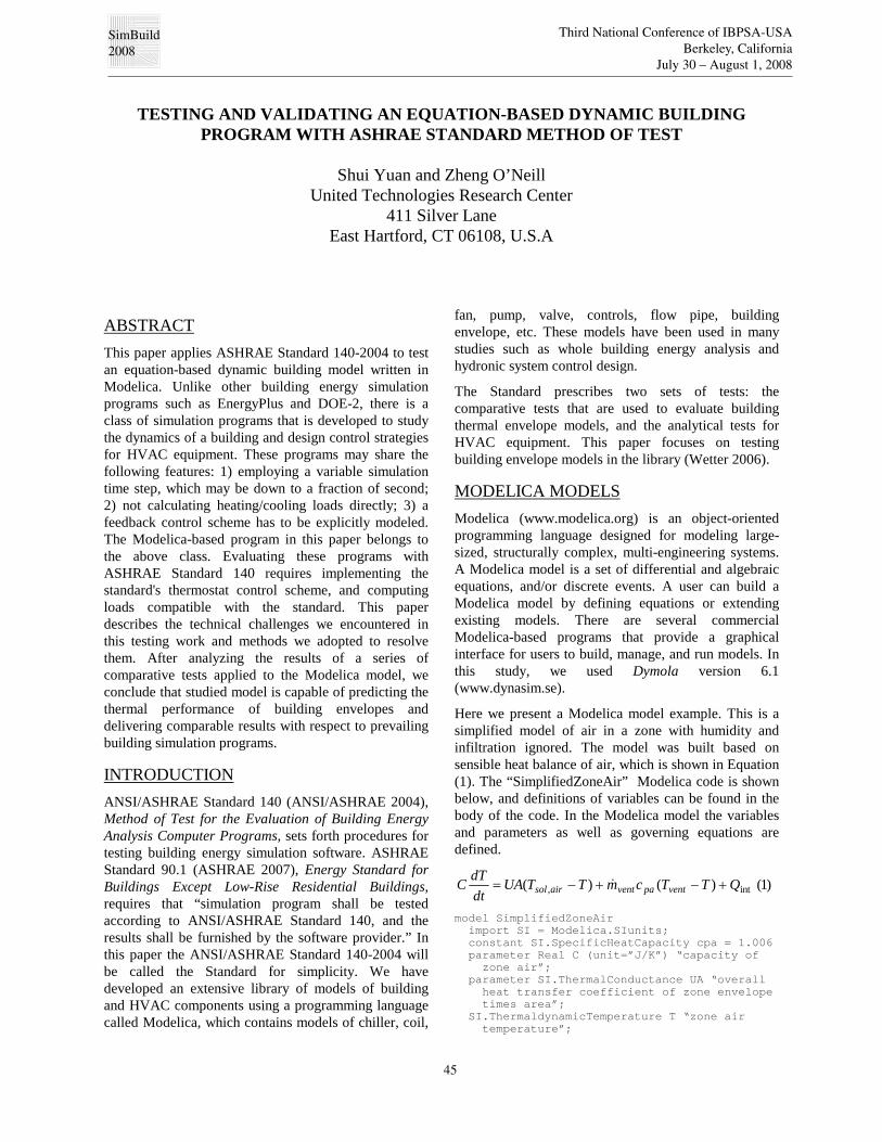
The Modelica models adopted a simplified model ofwindow that had a similar structure as the model ofopaque wall except that there is solar radiationtransmission through it and part of solar radiation isabsorbed by the glass. The other programs such asEnergyPlus use a much more sophisticated windowmodel. The simplified model for a double pane inModelica uses the transmitted solar radiation per unitarea through window as an input to a heat balancemodel(Wetter 2006). This transmitted solar radiationcan be obtained from building energy simulationprogram like EnergyPlus. This simplification led to alarge difference in the amount of net heat flow enteringa zone through a window as shown in Figure 8.

Figure 8 Net heat flow through one window over a year

Figure 8 shows differences between the Modelicamodel and EnergyPlus. The net heat flow in Modelica is16.6% less than that in EnergyPlus on average. We alsodid other root-cause analysis such as comparisons ofheat transfer rate wall by wall. We found that among allthe causes, the simplified window model is the primaryreason that the building loads calculated from theModelica model were closer to the lower bound andsmaller than those from EnergyPlus.

Implementation of the thermostat control scheme

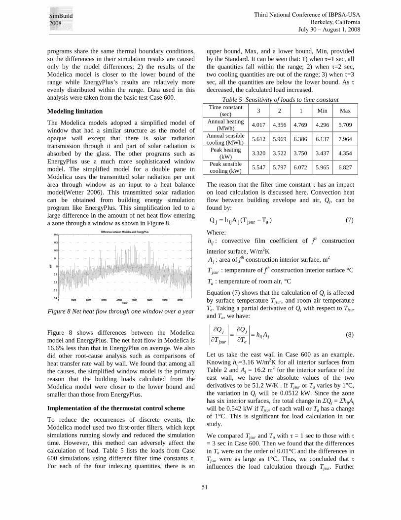
To reduce the occurrences of discrete events, theModelica model used two first-order filters, which keptsimulations running slowly and reduced the simulationtime. However, this method can adversely affect thecalculation of load. Table 5 lists the loads from Case600 simulations using different filter time constants τ.For each of the four indexing quantities, there is an

upper bound, Max, and a lower bound, Min, providedby the Standard. It can be seen that: 1) when τ=1 sec, allthe quantities fall within the range; 2) when τ=2 sec,two cooling quantities are out of the range; 3) when τ=3sec, all the quantities are below the lower bound. As τdecreased, the calculated load increased.

Table 5 Sensitivity of loads to time constantTime constant

(sec) 3 2 1 Min Max

Annual heating(MWh) 4.017 4.356 4.769 4.296 5.709

Annual sensiblecooling (MWh) 5.612 5.969 6.386 6.137 7.964

Peak heating(kW) 3.320 3.522 3.750 3.437 4.354

Peak sensiblecooling (kW) 5.547 5.797 6.072 5.965 6.827

The reason that the filter time constant τ has an impacton load calculation is discussed here. Convection heatflow between building envelope and air, Qj, can befound by:

)TT(AhQ ajsurjijj (7)

Where:ijh : convective film coefficient of jth construction

interior surface, W/m2KjA : area of jth construction interior surface, m2

jsurT : temperature of jth construction interior surface °C

aT : temperature of room air, °C

Equation (7) shows that the calculation of Qj is affectedby surface temperature Tjsur, and room air temperatureTa. Taking a partial derivative of Qj with respect to Tjsur

and Ta, we have:

jija

j

jsur

j AhT

Q

T

Q

(8)

Let us take the east wall in Case 600 as an example.Knowing hij=3.16 W/m2K for all interior surfaces fromTable 2 and Aj = 16.2 m2 for the interior surface of theeast wall, we have the absolute values of the twoderivatives to be 51.2 W/K . If Tjsur or Ta varies by 1°C,the variation in Qj will be 0.0512 kW. Since the zonehas six interior surfaces, the total change in ΣQj = ΣhijAj

will be 0.542 kW if Tjsur of each wall or Ta has a changeof 1°C. This is significant for load calculation in ourstudy.

We compared Tjsur and Ta with τ = 1 sec to those with τ= 3 sec in Case 600. Then we found that the differencesin Ta were on the order of 0.01°C and the differences inTjsur were as large as 1°C. Thus, we concluded that τinfluences the load calculation through Tjsur. Further

SimBuild2008



52

study of the DASSL algorithm’s effects is beyond thescope of this work. However, we think it is worthy ofinvestigations in the future. Figure 9 shows ∆Tjsur of theeast wall under two τ’s from March to April. The largestdifference is 0.96°C and the average is 0.40°C.

Figure 9 East wall interior surface temperaturedifference between different time constant τ

CONCLUSIONSComparative tests, specified in ASHRAE Standard 140-2004, were conducted in this study to evaluate thecapability of the Modelica model (Wetter, 2006).

We conclude that the Modelica building model iscapable of predicting the thermal performance ofbuilding envelopes because:

o 88.8% of the indexing quantities of thesimulations are in the range of example resultsfrom the Standard.

o The out-of-range quantities are close to therange of example results. In the worst casefrom basic tests, the result is only below thebound by 2.41%.

o The current results can be further improved byadopting tighter temperature controls, i.e.reducing the time constants τ of the first-orderfilters.

The current version of the Modelica model uses asimplified window, which transferred less heat flowthan the window model in EnergyPlus in our tests (by16.6% in Case 600).

Modelica is a programming language to model complexengineering dynamic systems by establishing a set ofdifferential and algebraic equations and discrete events.The thermostat control scheme in the Standard has to beimplemented explicitly, which may generate so many

discrete events that can significantly slow down orfreeze a simulation. A careful tradeoff must be madebetween simulation speed and accuracy. The Modelicamodel does not directly calculate loads. The user mustpostprocess the simulation data to calculate loads.

To enhance the capability of the Modelica model(Wetter, 2006), this study suggests using a moresophisticated window model and building a model toprocess raw weather data.

REFERENCES

ASHRAE. 2004. ANSI/ASHRAE Standard 140-2004.Standard Method of Test for the Evaluation ofBuilding Energy Analysis Computer Programs.

ASHRAE. 2007. ANSI/ASHRAE/IESNA Standard90.1-2007. Energy Standard for Buildings ExceptLow-Rise Residential Buildings.

www.dynasim.se

EnergyPlus. 2007. U.S. Department of Energy, EnergyEfficiency and Renewable Energy, Office ofBuilding Technologies. www.energyplus.gov

www.modelica.org

Wetter, M, 2006. Mutilzone Building Model forThermal Building Simulation in Modelica. Proc. ofthe 5th International Modelica Conference,Christian Kral and Anton Haumer(ed.), pp. 517-526. Vienna, Austria, 2006.

SIMBAD. 2007. http://www.cstb.fr/

NOMENCLATURE

jA : area of jth construction interior surface, m2

ih : interior combine surface coefficient, W/m2K

ijh : convective film coefficient of jth construction

interior surface, W/m2Koh : exterior combine surface coefficient, W/m2K

:ai specific enthalpy of room air, kJ/kg:ini specific enthalpy of infiltration, kJ/kg:m mass flow rate of infiltration, kg/sec

:LQ heating load (-) or sensible cooling load (+), kW:jQ heat flow from opaque walls, floor, ceiling, and

windows to air by convection, kW:cQ convective portion of internal heat gain, kW

aT : temperature of room air, °C

jsurT :temperature of jth construction interior surface °C

aaU : overall U-value from interior air to ambient

wU : U-value of double panes and air in between

testing and validating an equation-based … and validating an equation-based dynamic building...

Documents