testing and prediction of erosion-corrosion for corrosion ... dissertations/hernan... · testing...
TRANSCRIPT

T H E U N I V E R S I T Y O F T U L S A
THE GRADUATE SCHOOL
TESTING AND PREDICTION OF EROSION-CORROSION FOR CORROSION
RESISTANT ALLOYS USED IN THE OIL AND GAS PRODUCTION
INDUSTRY
byHernan E. Rincon
A dissertation submitted in partial fulfillment of
the requirements for degree of Doctor of Philosophy
In the discipline of Mechanical Engineering
The Graduate School
The University of Tulsa
2006

ii
T H E U N I V E R S I T Y O F T U L S A
THE GRADUATE SCHOOL
TESTING AND PREDICTION OF EROSION-CORROSION FOR CORROSION
RESISTANT ALLOYS USED IN THE OIL AND GAS PRODUCTION
INDUSTRY
by
Hernan E. Rincon
A DISSERTATION
APPROVED FOR THE DISCIPLINE OF
MECHANICAL ENGINEERING
By Dissertation Committee
_______________________________, Co-ChairJohn R. Shadley, Ph.D.
_______________________________, Co-ChairEdmund F. Rybicki, Ph.D.
_______________________________Kenneth P. Roberts, Ph.D.
_______________________________Dale C. Teeters, Ph.D.

iii
COPYRIGHT STATEMENT
Copyright © [2006] by [Hernan, E, Rincon]
All rights reserved. No part of this publication may be reproduced, stored in a
retrieval system, or transmitted, in any form or by any means (electronic, mechanical,
photocopying, recording or otherwise) with the prior written permission of the author.

iv
ABSTRACT
Rincon, Hernan Enrique (Doctor of Philosophy)
TESTING AND PREDICTION OF EROSION-CORROSION FOR CORROSIONRESISTANT ALLOYS USED IN THE OIL AND GAS PRODUCTION INDUSTRY(337pp.- Chapter 10)
Directed by Dr. John Shadley and Dr. Edmund Rybicki
( 328 Words)
The corrosion behavior of CRAs has been thoroughly investigated and
documented in the public literature by many researchers; however, little work has been
done to investigate erosion-corrosion of such alloys. When sand particles are entrained in
the flow, the degradation mechanism is different from that observed for sand-free
corrosive environment. There is a need in the oil and gas industry to define safe service
limits for utilization of such materials.
The effects of flow conditions, sand rate, pH and temperature on the erosion-
corrosion of CRAs were widely studied. An extensive experimental work was conducted.
using scratch tests and flow loop tests using several experimental techniques.
At high erosivity conditions, a synergistic effect between erosion and corrosion
was observed. Under the high sand rate conditions tested, erosivity is severe enough to
damage the passive layer protecting the CRA thereby enhancing the corrosion rate. In
most cases there is likely a competition between the rates of protective film removal due
to mechanical erosion and protective film healing.
v
Synergism occurs for each of the three alloys examined (13Cr and Super13Cr and
22Cr); however, the degree of synergism is quite different for the three alloys and may
not be significant for 22Cr for field conditions where erosivities are typically much lower
that those occurring in the small bore loop used in this research. Predictions of the
corrosion component of erosion-corrosion based on scratch test data compared
reasonably well to test results from flow loops for the three CRAs at high erosivity
conditions. Second order behavior appears to be an appropriate and useful model for
representing the repassivation process of CRAs.
A framework for a procedure to predict penetration rates for erosion-corrosion
conditions was developed based on the second order model behavior observed for the re-
healing process of the passive film of CRAs and on computational fluid dynamics (CFD)
simulations for erosion conducted for a direct impingement flow geometry. Reasonably
good agreement between the experimental and predicted erosion-corrosion penetration
rates was found.

vi
ACKNOWLEDGMENTS
I express my deep gratitude to my advisor Dr. Shadley, who consistently has
shown a great dedication and support, even while facing very difficult and painful times.
His guidance and encouragement really helped me overcome the challenges of this
research. I also give special thanks to Dr. Rybicki for his guidance and timely suggestions
which helped me throughout this research as well as in all aspects of my academic life. I
express sincere gratitude to Dr. Shadley and Dr. Rybicki for having provided me an
opportunity to work for a Ph.D. degree.
I am grateful for timely suggestions of Dr. Roberts. I also thank Dr. Teeters for
being part of my committee and providing his expertise. Special thanks goes to Senior
Technician Mr. Bowers for his expertise and support in the laboratory. I extend my
gratitude to the member companies of the Erosion/Corrosion Research Center. Special
thanks goes to Dr. McLaury and my colleague Yongli for their help throughout the CFD
work. I also express my fraternal appreciation to my friends Mauricio Papa, Jesus
Gonzalez and Rodrigo Chandia for their valuable encouragement and motivation since
the very beginning of this wonderful and challenging experience, as well as for providing
me with state of the art computers to speed up the CFD simulation. Thanks to all my
friends. This also gives me a great opportunity to express my deep appreciation, to my
wife Raicelina, to my son Ricardo, to my parents Eudelys, and Hernan, to my sister,
brother and nephew, Rossana, Enrique and Gabriel, and my coming baby for being part
of my life.

vii
DEDICATION
To my loving wife, my son Ricardo and my coming baby
viii
CONTENTS
COPYRIGHT STATETMENT……..………………..……….…….………......... iii
ABSTRACT…………………..………………………………………….……..... iv
ACKNOWLEDGMENTS…………………………………………………..……. vi
DEDICATION………………..……………………………………….………..... vii
CONTENTS……………………………………………………………..……….. viii
TABLE INDEX……………………………………………………………..……. xiii
FIGURE INDEX………………………………………………………………….. xv
CHAPTER 1 : INTRODUCTION…………..…………………………….…… 1
CHAPTER 2 : BACKGROUND AND LITERATURE REVIEW....…….….. 5
Basic Corrosion Concepts…..…………….……………………….…... 5
Concept and forms of corrosion…………………………….…... 5
Review of the Electrochemical Basis of Corrosion………… …...……. 7
Theory behind polarization measurements……………………… 8
Linear polarization resistance….…………..………...……..……. 11
Potentiodynamic polarization and Tafel constants……………….. 16
Active Passive Metal Behavior…………………………..……….…….. 17
Passive film……...………………………………………….……. 23
Maintenance and breakdown of passivity………………………... 26
Stainless Steel……………………...…………………………………….. 27
Alloying elements……………………………………………….... 27

ix
Flow velocity effects………………………………………….... 29
Flow pattern effects………………………………………….… 31
CO2 Corrosion Resistance of 13Cr Alloy………………….………... 33
Basic Erosion Concepts……………..…………………………….…. 36
Solid particle erosion………………………………………….. 37
Erosion of ductile materials…………….……………………... 39
Erosion of brittle materials………….……….……………...…... 39
Variables influencing erosion…….…………………………….. 40
Erosion-Corrosion……………..………….…….…………………...… 42
13Cr Alloy and Erosion-Corrosion………………………………..….. 46
Single phase liquid flow loop testing (high sand rates)……….... 51
Multiphase flow loop testing (high sand rates)……………...….. 52
CHAPTER 3: OBJECTIVES AND APPROACH……………………….…… 57
Research Objectives………….……………………………………….. 57
Research Approach…………………….……………………………… 58
CHAPTER 4: EXPERIMENTAL PROCEDURE AND TESTING
CONDITIONS…………………………………………………. 61
Scratch Test Experimental Setup……………………………………... 61
Test matrix..………………………………………………….….. 64
Erosion-Corrosion -Loop (Gas/Liquid/Sand Multiphase
Flow Loop)…………………………………………………………….. 64
Test cell…………………………………………………….….... 67
Test conditions…………………………………………….…..... 67
x
Erosion-Corrosion Liquid/Sand Loop (Microloop)…..………….….. 68
Direct impingement test cell…………………………………….. 71
Test conditions for liquid/sand loop test……………………… 74
Material tested…………………………………………………... 75
CHAPTER 5: SCRATCH TEST AS A SIMPLIFIED EROSION-
CORROSION TEST……………………………………….…. 76
Motivation for Doing Scratch Test…………………………………… 76
Data Reduction Technique……………………………………….…….. 77
Scratch Test Results………………………….……………………….. 81
Effect of pH on Scratch Test results………………………….…. 81
Effect of temperature on Scratch Test results............................... 85
Effect of type of material (CRA) on Scratch Test results……….. 90
Cumulative Thickness Loss and Repassivation Time…………..…... 92
CHAPTER 6: MULTIPHASE GAS/LIQUID/SAND FLOW LOOP
TESTING RESULTS…………………..…………………….... 100
Low Sand Rates (Multiphase Flow Loop Testing)………………….. 101
High Sand Rates (Multiphase Flow Loop Testing)…………………. 108
CHAPTER 7: COMPARISON OF SCRATCH TEST RESULTS WITH
FLOW LOOP TEST RESULTS…….………………………… 114
Scratch Test Data vs. Single Phase Liquid Flow Data………………. 116
Prediction of Erosion-Corrosion of CRAs using the Scratch Test….. 117
Single phase liquid flow…………………………..………………. 117

xi
Validation of Scratch Test Predictions of Erosion-Corrosion of
CRAs……………………………………………………………….…… 119
Multiphase flow……………………………………….………… 119
CHAPTER 8: SUBMERGED DIRECT IMPINGEMENT TEST:
SINGLE PHASE LIQUID FLOW…..……………………….... 122
Erosion-Corrosion Liquid/Sand Loop (Microloop)…………..…..….. 122
CHAPTER 9: EROSION-CORROSION MODEL……………………………. 136
General Approach……………………………………………..…….….. 136
Proposed Procedure for Estimating Ce-c……………..……………….. 139
Determination of the indented open area………………………… 142
Implementation of the second order model to determine the total
current……………………………………………………………. 143
Validation of the Erosion-Corrosion Prediction Model……………….. 150
Adjustment of the erosion prediction……………………….……. 150
Comparison between experimental data and predictions……….. 151
Some trends of predicted values………………………………..… 154
Effect of sand rate: comparison between experiments and
prediction trends……………………………………………..…. 154
Effect of temperature: comparison between experiments and
prediction trends…………………………………………….….. 159
Effect of material: comparison between experiments and
prediction trends…………………………………..……………. 160

xii
CHAPTER 10: SUMMARY, CONCLUSIONS AND
RECOMMENDATIONS………………………………………… 163
Summary……………..………………………………………………….. 163
Conclusions………………………………………………………………. 165
Scratch Tests…………………………………………….……….. 165
Multiphase gas/liquid/sand flow loop tests………………………. 166
Single phase liquid/sand flow loop testing (submerged direct
impingement test)……………………………………………… 168
Erosion-corrosion predictive procedure and model……………. 171
Recommendations………………………………………………………. 172
REFERENCES………………………………………………………………… 177
APPENDIX A………………………………………………………………….... 183
APPENDIX B………………………………………………………………….. 196
APPENDIX C……………………………………………………………….…. 198
APPENDIX D……………………………………………………………….…. 212
APPENDIX E…………………………………………………………………. 228
APPENDIX F …………………………………………………………….…… 233

xiii
LIST OF TABLES
Table 4-1. Test conditions for erosion and erosion-corrosion tests. .............................. 68
Table 4-2. Test conditions for erosion and erosion-corrosion tests ............................... 74
Table 4-3. The chemical composition of 13Cr. .............................................................. 75
Table 4-4. The chemical composition of Super 13Cr. ................................................... 75
Table 4-5. The chemical composition of the 22Cr. ........................................................ 75
Table 5-1. Repassivation times in minutes for 13Cr at different test conditions
using current data time series approach. ..................................................... 95
Table 5-2. Repassivation times in minutes for 13Cr at different test conditions
using second order kinetics approximation. ................................................ 96
Table 5-3. Repassivation times in minutes at pH = 4 and the three temperatures
for Super 13Cr and 22Cr using both approaches, current data time
series approach and second order kinetics approximation. ......................... 96
Table 6-1. Erosion-corrosion (EC), pure erosion (E) and corrosion components
(Ce-c) of the erosion-corrosion penetration rates for 3 alloys tested at
similar conditions. 76oF, pH 4, Vsg = 20 ft/s, Vsl = 1.4 ft/s, 30 lb/day
of sand. ...................................................................................................... 111
Table 6-2. Erosion-corrosion (EC), pure erosion (pureE) and corrosion
components (CEC) of the erosion-corrosion penetration rates for 3

xiv
alloys tested at similar conditions. 150oF, pH 4, Vsg = 20 ft/s, Vsl =
1.4 ft/s, 30 lb/day of sand . ........................................................................ 112
Table 7-1. Erosion-corrosion penetration rates and corrosion components (Ce-c)
of the erosion-corrosion penetration rate for 13Cr at different
temperatures. (Vl = 15 ft/s (4.6 m/s), PCO2=50 psig (344.7 kPa),
Brine 3%, about 3,500 lb sand /day (1,587.6 kg sand /day)). ................... 116
Table 7-2. Comparison of relative severity of the corrosion component of the
erosion-corrosion between single phase liquid loop tests and scratch
tests for 13Cr. ............................................................................................ 117
Table 7-3. Actual and predicted values of the corrosion component (Ce-c) of the
erosion-corrosion penetration rates for 3 alloys tested at similar
conditions (76oF, pH 4) ............................................................................. 121
Table 7-4. Actual and predicted values of the corrosion component (CEC) of the
erosion-corrosion penetration rates for 3 alloys tested at similar
conditions (150oF, pH 4). .......................................................................... 121
Table 8-1. Summary of corrosion component rates of erosion-corrosion Ce-c;
erosion-corrosion rates, E-C; and pure Erosion rates E, obtained
experimentally. 150F and 4.3 pH. ........................................................... 135
Table 8-2. Summary of experimental values obtained for the current Io. 150F
and 4.3 pH. ................................................................................................ 135

xv
LIST OF FIGURES
Figure 2-1. Corrosion process showing anodic and cathodic current
components.33 ................................................................................................ 9
Figure 2-2. Standard anodic polarization curve (430 stainless steel in 1 N
H2SO4) showing a typical active passive transition behavior. .................... 19
Figure 2-3. Schematic of active-passive transition. Potentiostatic anodic curve
“jklm”; hydrogen evolution reaction, curve “hi”; low concentration
of dissolved oxygen, curve “defg”; high concentration of dissolved
oxygen, curve “abc”. ................................................................................... 21
Figure 2-4. Theoretical and actual potentiodynamic plots of active passive
metals. ......................................................................................................... 23
Figure 2-5. Decay of passive corrosion rate measured by potentiostatic current.
31 .................................................................................................................. 25
Figure 2-6. Log-log plot of data from Figure 2-5 at extended times. 31 ......................... 26
Figure 2-7. Effect of chromium content on anodic polarization of Fe-Ni alloys ............ 29
Figure 2-8. Major categories of wear based on their fundamental mechanisms. 49 ....... 37
Figure 2-9. Schematic of the effect of the impingement angle on erosion rate of
ductile and brittle materials......................................................................... 40
Figure 2-10. Schematic of polarization curves for type 316 stainless steel
showing the effect of percent solids sand slurry.38...................................... 46

xvi
Figure 2-11. Plot of the mass loss rate vs. normalized distance from the pipe
expansion at different flow rates. (60oC, 3 bar CO2 and 1000 ppm of
sand (Re number 5.7 105 correspond to a flow velocity of 5.7 m/s).
52 .................................................................................................................. 47
Figure 2-12. Influence of various sand concentrations on the mass loss rate along
the pipe length at a flow rate of 3.5 m/s. 52 ................................................. 48
Figure 2-13. Thickness loss versus time for a 13Cr alloy exposed to CO2
saturated brine containing sand particles. 53................................................ 49
Figure 2-14. Comparison of penetration rates for pure erosion and erosion-
corrosion at different temperatures by the weight-loss method
(single phase liquid flow, Vl =15 ft/s). 58..................................................... 52
Figure 2-15. Penetration rates for pure erosion and erosion-corrosion tests of
13Cr in multiphase flow conditions (Vsg = 97 ft/s, Vsl = 0.2 ft/s).57........... 53
Figure 2-16. Comparison among penetration rates for pure Corrosion, pure
Erosion and Erosion-Corrosion processes (Vsg= 97 ft/s, Vsl= 0.2
ft/s). 59 .......................................................................................................... 54
Figure 4-1. Layout of the electrochemical cell for Scratch Test.................................... 62
Figure 4-2. Set-up for electrochemical measurements for Scratch Test...........................63
Figure 4-3. Schematic of the Erosion-Corrosion Flow Loop ...........................................66
Figure 4-4. Photograph of the test section of the Erosion-Corrosion loop with
the ER probe set in place (left). Sensor element of the 13Cr ER
Probe (right). ................................................................................................67
Figure 4-5. Schematic of the Microloop. ........................................................................72

xvii
Figure 4-6. Schematic of the test cell section for the Microloop indicating
positions of target working electrode (WE1) and auxiliary working
electrode (WE2). ...........................................................................................73
Figure 4-7. Schematic of the direct impingement test cell for the Microloop ................73
Figure 5-1. Anodic current decay during the scratch repassivation process. .................. 77
Figure 5-2. Data showing a linear relation between 1/I and time.................................... 78
Figure 5-3. Comparison between TLactual and TLcal for 13Cr alloy. ........................... 80
Figure 5-4. Effect of pH on the decay of the anodic current after a scratch has
been made on the surface of a 13Cr Alloy.................................................. 83
Figure 5-5. Effect of pH on the decay of the anodic current after a scratch has
been made on the surface of a Super 13Cr Alloy........................................ 83
Figure 5-6. 1/I vs. t for 13Cr from the raw scratch test data in Figure 5-4...................... 84
Figure 5-7. 1/I vs. t for 13Cr from the raw data in Figure 5-5......................................... 85
Figure 5-8. Effect of temperature on the decay of the anodic current after a
scratch has been performed on the surface of a 13Cr Alloy. ...................... 86
Figure 5-9. Effect of temperature on the cumulative thickness loss experienced
by 13Cr after being scratched at pH=4.0..................................................... 87
Figure 5-10. Effect of temperature on the decay of the anodic current after a
scratch has been performed on the surface of a Super 13Cr Alloy. ............ 87
Figure 5-11. Effect of temperature on the decay of the anodic current after a
scratch has been performed on the surface of a 22Cr Alloy. ...................... 88
Figure 5-12. 1/I vs. t for 13Cr from the raw data in Figure 5-8. ...................................... 89
Figure 5-13. 1/I vs. t for 13Cr from the raw data in Figure 5-10..................................... 89

xviii
Figure 5-14. 1/I vs. t for 13Cr from the raw data in Figure 5-11..................................... 90
Figure 5-15. Decay of the anodic current for three different alloys................................. 91
Figure 5-16. Comparison of 1/I vs. t for 13Cr and Super 13Cr at 150°F, 22Cr at
pH 4 is also included. .................................................................................. 91
Figure 5-17. Comparison of the cumulative thickness loss after 200 seconds for
the three CRAs at pH = 4 and different temperatures. ................................ 93
Figure 5-18. Effect of temperature on the ratios of the Thickness Loss of 13Cr to
Super 13Cr and to 22Cr............................................................................... 94
Figure 5-19. Effect of pH and temperature on the repassivation times of 13Cr at
different test conditions. Data for Super 13Cr and 22Cr at pH 4 and
the three temperatures are also included. .................................................... 98
Figure 5-20. Effect of pH and temperature on the repassivation times of Super
13Cr at different test conditions. Data for 22Cr at pH 4 and the three
temperatures are also included. ................................................................... 98
Figure 5-21. Comparison of the repassivation times for the three CRAs at pH 4
and different temperature. ........................................................................... 99
Figure 5-22. Comparison between repassivation times obtained from actual data
and estimated from the second order kinetic approximation. ..................... 99
Figure 6-1. Pure erosion test for 13Cr under sand-N2-distilled water flow system
(Vsg=60 ft/s, Vsl= 0.2 ft/s) at 150oF and low sand rate (15 lb/day). .......... 103
Figure 6-2. Erosion-corrosion test for 13Cr under sand-CO2-Brine flow system
(Vsg=60 ft/s, Vsl= 0.2 ft/s) at 150oF and low sand rate (15 lb/day). ........ 104

xix
Figure 6-3. Penetration rate for pure Erosion and Erosion-Corrosion tests of
13Cr in multiphase flow testing at 76oF. (The errors bars on the
average represent the 95% confidence interval on the mean value.) ........ 105
Figure 6-4. Penetration rate for pure Erosion and Erosion-Corrosion tests of 13Cr
in multiphase flow testing at 150oF. (The errors bars on the average
represent the 95% confidence interval on the mean value.)...................... 107
Figure 6-5. Erosion-corrosion (EC), pure erosion (pure E) and corrosion
component (CEC) of the erosion-corrosion penetration rates for data
shown in Table 6-1. ................................................................................... 111
Figure 6-6. Erosion-corrosion (EC), pure erosion (pureE) and corrosion
component (CEC) of the erosion-corrosion penetration rates for data
shown in Table 6-2.................................................................................... 112
Figure 7-1. Corrosion component of the erosion-corrosion process for 13Cr
(actual flow liquid loop data), Super 13Cr and 22Cr (data
extrapolated with scratch data) at pH 4 and 3 different temperatures....... 118
Figure 8-1. Current response for Super 13Cr exposed to CO2 saturated brine
containing sand.......................................................................................... 125
Figure 8-2. Comparison between current responses for Super 13Cr exposed to
CO2-saturated brine at similar environmental and flow conditions
but different sand rates. ............................................................................. 126
Figure 8-3. Comparison between current responses for Super 13Cr exposed to
CO2-saturated brine at similar environmental conditions but
different flow velocities and sand rates..................................................... 127

xx
Figure 8-4. Anodic current decay for Super 13Cr alloy after sand is removed
from the test cell loop. ............................................................................... 128
Figure 8-5. A linear behavior between 1/I and time after sand is removed from
the test cell loop......................................................................................... 129
Figure 8-6. Actual data and second order model for the anodic current decay after
sand is removed from of the test cell loop. ............................................... 130
Figure 8-7. Effect of sand rate on the anodic current decay of Super 13Cr alloy. ........ 131
Figure 8-8. Effect of sand rate on the linear behavior for 1/I with time after sand
is removed from the test cell loop. ............................................................ 131
Figure 8-9. Effect of pH on the anodic current decay of 13Cr alloy. ............................ 132
Figure 8-10. Comparison of the resultant metallic surfaces of the target specimen
of 13Cr and Super 13Cr exposed to different erosion-corrosion
conditions. ................................................................................................. 134
Figure 9-1. Schematic of a particle impingement on a passive alloy. ........................... 140
Figure 9-2. Generic plot for the total current and individual current transients of
6 different impacts taking place in a numerical cell of the target
specimen.................................................................................................... 145
Figure 9-3. Generic plot for the total current generated in a cell due to total
particle impact. .......................................................................................... 146
Figure 9-4. Typical behavior of the total current produce in a numerical cell due
to the particle impact. The cell is hit at an impact frequency of 74
particles per second. .................................................................................. 147
Figure 9-5. Flow diagram to estimate E, Ce-c, & EC .................................................. 149
xxi
Figure 9-6. Comparison between measured erosion and erosion-corrosion
penetration rates (by weight loss) and those predicted by the
proposed model. ........................................................................................ 151
Figure 9-7. Comparison between measured corrosion component penetration
rates (by LPR) and those predicted by the proposed model...................... 153
Figure 9-8. Comparison between measured total current values (A) and those
predicted by the proposed model. ............................................................. 153
Figure 9-9. Prediction trends with sand rate of pure erosion, E for several flow
velocities.................................................................................................... 155
Figure 9-10. Prediction trends with sand rate of pure erosion, E and corrosion
component of erosion-corrosion, Ce-c for Super 13Cr at two flow
velocities.................................................................................................... 156
Figure 9-11. Comparison between 13Cr and Super 13Cr prediction trends with
sand rate of pure erosion, E and corrosion component of erosion-
corrosion, Ce-c. ......................................................................................... 157
Figure 9-12. Effect of pH and temperature on the prediction trends with sand rate
of the corrosion component of erosion-corrosion, Ce-c for 13Cr. ............ 158
Figure 9-13. Comparison between experimental data and predicted trends with
temperature of the erosion-corrosion of 13Cr. All data normalized to
room temperature values. .......................................................................... 160
Figure 9-14. Comparison between experimental data and predicted trends with
temperature of the erosion-corrosion of Super 13Cr. All data
normalized to room temperature values. ................................................... 161
xxii
Figure 9-15. Comparison between experimental data and predicted trends with
temperature of the erosion-corrosion of 22Cr. All data normalized to
room temperature values. .......................................................................... 161
Figure 9-16. Comparison between experimental data and predicted trends of the
erosion-corrosion, EC of the three CRAs at two different
temperatures. All data normalized to 13Cr at room temperature
value. ......................................................................................................... 162

1
CHAPTER 1
INTRODUCTION
Corrosion has an important impact on the total cost of oil and gas production. Its
direct and indirect costs in the US were estimated to be several billions of dollars,
according to a 1999 U.S. Congressional study.1 In particular, initial purchase costs and
maintenance costs for controlling corrosion of production tubing, pipelines and other
equipment, is one of the oldest material performance problems facing the oil and gas
industry.
From the diversity of corrosion related problems, carbon dioxide (CO2) corrosion
of carbon steel is probably the material degradation mechanism most extensively
assessed in this industry for the last 30 years. During this time, many models directed
towards predicting the physics involved in the CO2 corrosion process of carbon steel have
been established. Empirical laboratory models, empirical field models and mechanistic
models have been developed in this area, and many parameters have been taken into
account, such as effects of CO2 pressure, temperature, pH, chloride content, and
hydrodynamics among others. Today, CO2 corrosion is a well understood phenomenon;
however, the dynamics of the oil business have led the oil and gas industry to the

2
production of wells of greater and greater depths with increasing severity of the service
conditions.
Sometimes, it may be more economical in the long term to use corrosion
resistance alloys (CRA) instead of the normally used carbon steel, for which expensive
chemical treatment programs are often required. Recently, we have witnessed the
increasing use of CRAs in the oil and gas industry. In a sweet environment,2 the most
widely used corrosion resistance alloy is 13Cr and its modified types. The main reasons
are its excellent corrosion resistance in a CO2 corrosion environment and its low cost
compared with other CRAs such as duplex stainless steel.3
Numerous research papers were published in recent years to investigate the
corrosion behavior of 13Cr or its modified types at different service conditions.4-21 The
13Cr alloy has an excellent CO2 corrosion resistance. In fact, the effects of high gas
velocity and corrosion by CO2 experienced with carbon steels have been reduced to low
levels or virtually eliminated by alloying with 12 percent or more chromium.22 However,
when sand particles are entrained in the flow, the metal loss mechanism is different.
Recently, the need has arisen to define safe service limits for utilization of such materials
in corrosive oil and gas environments which may contain sand particles. However, little
work has been done to investigate the joint effect of erosion and erosion-corrosion of
such alloys.
Erosion by solid particle impingement, without any additional chemical
degradation components, is a complex problem by itself. The American Petroleum
Institute standard, API RP-14E, has been used for many years as the main guide for
designing and operating oil and gas production piping systems based on an estimation of

3
limiting erosional velocities. Its applicability and limitations have been widely discussed
and published.23-30 Researchers have done extensive experimental and modeling work to
generalize and improve estimates of erosional velocities when solid particles are
suspended in the flow. When CO2 corrosion and solid particle impingement are acting
together on the metallic surface, the metal loss rates experienced are often significantly
higher than those observed when pure corrosion and pure erosion are taken separately.
The mixed degradation mode inherent in the sand-erosion/CO2-corrosion
mechanism does not allow the study to focus on only one mechanism. Besides,
dominating parameters driving the material degradation may be different from the CO2
corrosion or pure erosion mechanisms by themselves. Hence, extensive research work is
required to address this problem. Some work also has been directed toward obtaining a
better understanding of the combined erosion-corrosion process.
Addressing these needs is challenging, especially when taking into account both
the complexity of the chemi-mechanical mechanism presented and the diversity of
service conditions found in oil and gas production. The complexity of the mechanisms
involved in erosion-corrosion of metals, based on the large amount of variables involved,
has been remarked on by several authors.
This research work has been directed towards the study of the effect of sand on
the erosion-corrosion of CRAs, including 13Cr, Super 13Cr (S13Cr) and 22Cr. The
effects of flow conditions, sand rate, pH and temperature on the characterization of the
erosion-corrosion of 13Cr were widely studied, and a direct comparison of 13Cr vs.
Super 13Cr and 22Cr under similar erosion-corrosion conditions was also made. To
characterize the erosion, corrosion and erosion-corrosion behavior of the mentioned

4
CRAs, several experimental techniques were utilized such as weight loss (WL), electrical
resistance (ER), linear polarization resistance (LPR), potentiodynamic scan (PD), and
scratch test (ST) which may be seen as a modified electrochemical noise technique. The
latter, along with computational fluid dynamics (CFD) simulations, provided the
foundation for a procedure built to predict erosion-corrosion rates of CRAs in brine flows
containing sand. Lastly, experimental results and predicted values were compared for a
broad range of conditions with encouraging results.
5
CHAPTER 2
BACKGROUND AND LITERATURE REVIEW
Basic Corrosion Concepts
Concept and forms of corrosion
The material degradation of a metal as a consequence of a chemical reaction
between a metal and its environment is called corrosion. Metal atoms are normally
present in nature as minerals (chemical compounds). The amount of energy needed to
extract metals from their minerals during chemical reactions is the same as that involved
in the corrosion process. Most of the time, corrosion occurs spontaneously, returning the
metal to its combined state in chemical compounds that are similar to the mineral from
which the metals were extracted.31
Several forms of corrosion have been widely studied and classified by different
authors. A full discussion of all forms of corrosion is beyond the scope of this
dissertation, and particular attention will be given to research efforts in the area of
erosion-corrosion phenomena. However, some of these forms are listed below.
Uniform Corrosion Galvanic Corrosion Crevice Corrosion Pitting Corrosion
6
Environmentally Induced Cracking Intergranullar Corrosion Dealloying Erosion-Corrosion
In general, uniform corrosion may be considered as the more common type of corrosion
found as well as the easiest to predict and control. The different types of localized
corrosion are more insidious and difficult to predict and control. While localized
corrosion may not consume as much material, penetration and failure are more rapid and,
hence, is generally considered a more severe type of corrosion.
Uniform loss of metal is also a common form of corrosion observed in the oil
industry. However, in oilfield operations, metal loss is frequently localized in the form of
discrete pits or larger localized areas. Additionally, stages of incipient corrosion in metals
often provide suitable conditions for metal cracking without perceptible loss of material,
and then metallurgical factors become predominant.32 Some alloys often used in the oil
industry owe their corrosion resistance to the formation and persistence of a protective
layer. Removal of this layer at local areas can lead to accelerated attack. Extremely high
velocity flow and intense turbulence may erode away the protective layer to expose fresh
metal which then can be corroded at a faster rate. Whether localized or uniform
corrosion, nearly all metallic corrosion processes involve transfer of electronic charge in
aqueous solutions so their electrochemical nature is the same for all forms of corrosion. It
is thus important to discuss this process.

7
Review of the Electrochemical Basis of Corrosion
Most metal corrosion occurs by means of electrochemical reactions taking place
at the interface between the metal and an electrolyte solution. Corrosion normally occurs
at a rate determined by equilibrium between opposing electrochemical reactions. The
first is the anodic reaction, in which a metal (M) is oxidized, releasing electrons (e-) and
is represented by,
neMM n (2-1)
The other is the cathodic reaction, in which a solution species (often H+ or O2) is reduced,
removing electrons from the metal. Equilibrium between hydrogen gas and acid solutions
is represented by,
222 HeH (2-2)
or a reaction equivalent to Eq. (2.2) in neutral or alkaline solutions.
OHHeOH 222 22 (2.3)
As the potential becomes more positive, another reaction involving water becomes
thermodynamically feasible. In acid solutions, oxygen reduction is represented by
OHeHO 22 244 (2.4)
while in neutral or alkaline solutions
.442 22 OHeOHO (2.5)

8
When these two anodic (equation (2-1)) and cathodic (equations (2-2), (2-3), (2-4) or
(2.5)) reactions are in equilibrium, the flow of electrons from each reaction is balanced,
and no net electron flow (electrical current) occurs. Both reactions can take place on a
single metal or on two different electrically connected metals.31
Electrochemical reactions like those described by equations (2-1) and (2-2)
proceed only at limited rates. If electrons are made available in abundance, according to
equation (2-1), the potential at the surface becomes more negative. This means that an
excess of electrons (with their negative charges) has accumulated at the metal/solution
interface. Not all the available electrons waiting at the surface can be accommodated
because the reduction reaction is too slow. This negative potential change is called
cathodic polarization. Similarly, a deficiency of electrons in the metal/solution interface
produced by a positive potential change is called anodic polarization. As the deficiency
(polarization) increases, the tendency also increases for anodic dissolution. Anodic
polarization can be thought of as a driving force for corrosion by the anodic reaction,
equation (2-1). When the surface potential measures more positive, the oxidizing power
of the solution increases because the anodic polarization is greater.31
Theory behind polarization measurements
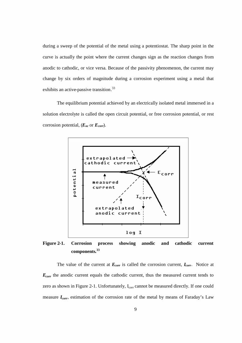
Figure 2-1 illustrates the process mentioned above. The ordinate represents
potential and the abscissa represents the logarithm of absolute current. According to the
mixed potential theory, the theoretical currents for the anodic and cathodic reactions vary
linearly with surface potential and are shown as straight lines in Figure 2-1.33 The curved
line is the actual current as would be experimentally measured, which represents the total
current that is the sum of the anodic and cathodic currents. This is the current measured
9
during a sweep of the potential of the metal using a potentiostat. The sharp point in the
curve is actually the point where the current changes sign as the reaction changes from
anodic to cathodic, or vice versa. Because of the passivity phenomenon, the current may
change by six orders of magnitude during a corrosion experiment using a metal that
exhibits an active-passive transition.33
The equilibrium potential achieved by an electrically isolated metal immersed in a
solution electrolyte is called the open circuit potential, or free corrosion potential, or rest
corrosion potential, (Eoc or Ecorr).
Figure 2-1. Corrosion process showing anodic and cathodic current
components.33
The value of the current at Ecorr is called the corrosion current, Icorr. Notice at
Ecorr the anodic current equals the cathodic current, thus the measured current tends to
zero as shown in Figure 2-1. Unfortunately, Icorr cannot be measured directly. If one could
measure Icorr, estimation of the corrosion rate of the metal by means of Faraday’s Law
10
would be straight forward. However, Icorr can be estimated using electrochemical
techniques.
Icorr and corrosion rates are a function of many variables including type of metal,
metal history, surface finishing, solution composition, solution pH, temperature,
dissolved gases, hydrodynamics of the system, and many others. In practice, many metals
form an oxide layer on their surface as they corrode. If the oxide layer significantly
inhibits the corrosion process, the metal is said to passivate. In some cases, local areas of
the passive film break down allowing significant metal corrosion to occur in a small area
leading to localized corrosion with higher localized penetration rates.
Reactions in the corrosion process are electrochemical. Thus electrochemical
techniques are ideal for the study of the corrosion processes. In electrochemical studies,
a metal sample with a surface area of a few square centimeters is used to model the metal
in a corroding system. This metal sample is often called the working electrode. The metal
sample is immersed in a solution that simulates the real environment of the system
studied. For the standard three-electrode system, two more electrodes are immersed in the
solution, namely the reference electrode and the counter electrode (also called the
auxiliary electrode). The reference electrode is commonly a low polarizable, and very
stable, electrode which serves as a reference for the metal sample potential
measurements. The counter electrode is commonly an inert electrode that closes the
electrical circuit. It serves as the substrate where the cathodic reaction occurs while the
anodic reaction is taking place in the working electrode (metal sample) or vice versa. All
the electrodes are connected to a device called a potentiostat. A potentiostat allows you

11
to change the potential of the metal sample in a controlled manner and measure the
current that flows as a function of the applied potential.
Controlled potential experiments, such as linear polarization resistance (LPR) and
potentiodynamic polarization scan (PD), are used to perturb the equilibrium corrosion
process by polarizing the sample. The response (current) of the metal sample due to the
polarization is measured. Some models of the sample’s current behavior have been
developed to estimate corrosion rates from the current response.33
Linear polarization resistance
In the previous section, it was pointed out that Icorr cannot be measured directly.
In many cases, one can estimate it from current versus voltage data. As mentioned before,
current can be measured as potential increases, and a log current versus potential curve
can be plotted over a range of about one half volt. The voltage scan is centered on Ecorr.
Then the measured data can be fitted to a theoretical model of the corrosion process.
The model usually used for the corrosion process assumes that the rates of both
the anodic and cathodic processes are controlled by the kinetics of the electron transfer
reaction at the metal surface. An electrochemical reaction under kinetic control obeys the
Tafel equation as follows.33
)(303.2
exp 00
EEII (2-6)
where, I is the current resulting from the reaction, Io is a reaction dependent constant
called the exchange current, E is the electrode potential, Eo is the equilibrium potential
12
(constant for a given reaction) and is the reaction's Tafel constant with units of
volts/decade (constant for a given reaction).
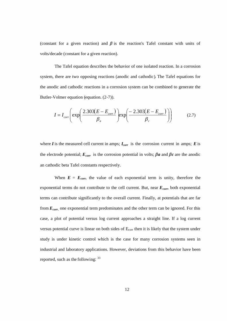
The Tafel equation describes the behavior of one isolated reaction. In a corrosion
system, there are two opposing reactions (anodic and cathodic). The Tafel equations for
the anodic and cathodic reactions in a corrosion system can be combined to generate the
Butler-Volmer equation (equation. (2-7)).
c
corr
a
corrcorr
EEEEII
303.2
exp303.2
exp (2.7)
where I is the measured cell current in amps; Icorr is the corrosion current in amps; E is
the electrode potential; Ecorr is the corrosion potential in volts; a and c are the anodic
an cathodic beta Tafel constants respectively.
When E = Ecorr, the value of each exponential term is unity, therefore the
exponential terms do not contribute to the cell current. But, near Ecorr, both exponential
terms can contribute significantly to the overall current. Finally, at potentials that are far
from Ecorr, one exponential term predominates and the other term can be ignored. For this
case, a plot of potential versus log current approaches a straight line. If a log current
versus potential curve is linear on both sides of Ecorr then it is likely that the system under
study is under kinetic control which is the case for many corrosion systems seen in
industrial and laboratory applications. However, deviations from this behavior have been
reported, such as the following: 33
13
Concentration polarization: This is the condition for which the rate of a reaction is
controlled by the rate at which reactants arrive at the metal surface. Cathodic reactions
often show concentration polarization at higher currents for which diffusion of the
oxygen or hydrogen ion is slower than the kinetically controlled reaction rate.
Oxide formation: Formation of oxides on the surface of the metal, which may or
may not lead to passivation, can alter the surface of the sample being tested. The original
surface and the altered surface may have different values for the Tafel constants.
Mixed control process: where more than one cathodic, or anodic, reaction occurs
simultaneously may complicate the model. An example of this is the simultaneous
reduction of oxygen and hydrogen ion in aerated acid solutions.
Other effects that alter the surface, such as preferential dissolution of one alloy
component, or adsorption of charged chemical species to the metallic surface, can also
cause problems in interpreting electrochemical measurement data.
In classic Tafel analysis, linear portions of a potential versus log current plot are
extrapolated back to their intersection (see Figure 2-1). The value of either the anodic or
the cathodic current at the intersection is Icorr. Unfortunately, for many real world
corrosion systems, a sufficient linear region to permit accurate extrapolation is not
observed. Therefore, this type of analysis is not often used to estimate corrosion rates but
rather to learn something about the mechanism driving the corrosion process.
Equation (2-7) can be further simplified by restricting the potential to be very near
to Ecorr. For potential E sufficiently close to Ecorr, the current versus voltage curve
approximates a straight line. The slope of this line is called the polarization resistance,
14
Rp, because it has the units of resistance (ohms). An estimate of the corrosion current can
be obtained by combining the Rp value with estimates of the beta coefficients.
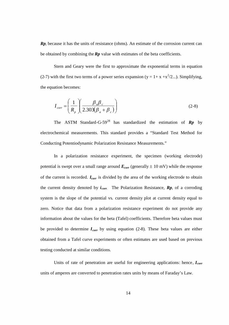
Stern and Geary were the first to approximate the exponential terms in equation
(2-7) with the first two terms of a power series expansion (y = 1+ x +x2/2...). Simplifying,
the equation becomes:
ca
ca
pcorr R
I
303.2
1(2-8)
The ASTM Standard-G-5928 has standardized the estimation of Rp by
electrochemical measurements. This standard provides a “Standard Test Method for
Conducting Potentiodynamic Polarization Resistance Measurements.”
In a polarization resistance experiment, the specimen (working electrode)
potential is swept over a small range around Ecorr (generally 10 mV) while the response
of the current is recorded. Icorr is divided by the area of the working electrode to obtain
the current density denoted by icorr. The Polarization Resistance, Rp, of a corroding
system is the slope of the potential vs. current density plot at current density equal to
zero. Notice that data from a polarization resistance experiment do not provide any
information about the values for the beta (Tafel) coefficients. Therefore beta values must
be provided to determine Icorr by using equation (2-8). These beta values are either
obtained from a Tafel curve experiments or often estimates are used based on previous
testing conducted at similar conditions.
Units of rate of penetration are useful for engineering applications: hence, Icorr
units of amperes are converted to penetration rates units by means of Faraday’s Law.

15
Assume an electrolytic dissolution reaction involving a chemical species, S:
neSS n (2-9)
According Faraday's Law, current flow is related to mass via.
nFMQ (2-10)
where, Q is the charge in coulombs resulting from the reaction of species S, n is the
number of electrons transferred per molecule or atom of S, F is Faraday's constant
(96,486.7 coulombs/mole), and M is the number of moles of species S reacting.
The equivalent weight (EW) is the mass of species S that will react with one
96,500 coulombs (Faraday’s constant) of charge. For an atomic species, EW = AW/n
(where AW is the atomic weight of the species). Recall that M = W/AW and substituting
into equation. (2.10) gives:
FEWQW (2-11)
where W is the mass of species S that has reacted.
If corrosion occurs uniformly across a metal surface, the corrosion rate can be
calculated in units of distance per year. Corrosion rate, C can be obtained from weight
loss data in a simple form by applying equation (2-12). The metal density, , and the
sample area, A, are needed as input. For constant current, the charge is given by Q = I t,
where t is the time in seconds and I is a current. The current density is calculated as i =
I/A. Substituting the value of Faraday's constant, Eq. (2-11) becomes.
EWi
kC corr (2.-12)

16
where C is the corrosion rate, icorr is the corrosion current density in A/cm2, EW is the
equivalent weight in grams/equivalent; is density in grams/cm3, k is a constant that
defines the units for the corrosion rate, k = 3.272 x 10⁻³ for mm/year and k = 0.1288
millinches/year (mpy).
The equivalent weight for a complex alloy undergoing uniform dissolution can be
calculated as the weighted average of the equivalent weights of the alloys components.
Mole fraction is used instead of mass fraction as the weighting factor. The estimation of
corrosion rate by this means has been widely accepted and ASTM Standard-G-10234,
“Standard Practice for Calculation of Corrosion Rates and Related Information from
Electrochemical Measurements”, which can be consulted for further information.
Potentiodynamic polarization and Tafel constants
Potentiodynamic polarization curves are used to determine corrosion behavior of
metal specimens in aqueous environments by studying their current-potential
relationships. The specimen potential is scanned slowly, as in linear polarization
resistance experiments, but over a larger range of potentials. A complete current-potential
plot of a specimen can be measured in a few hours or in some cases in a few minutes
depending on the scan rate and the potential range to be covered.
Suppose the potential is forced from Ecorr to more positive values (anodic region)
by using a potentiostat. That is moving towards the top of the graph in Figure 2-1. This
will increase the rate of the anodic reaction, ia, (that means increase the corrosion rate)
and decrease the rate of the cathodic reaction, ic. Since the anodic and cathodic reactions
are no longer balanced, a net current, imeasured will flow from the counter electrode

17
(through the electronic circuit) into the metal sample (working electrode). The sign of
this current is positive by convention. If the potential is taken far enough from Ecorr the
cathodic reaction current will be negligible and the measured current (imeasured) will
represent the anodic reaction alone. In Figure 2-1, notice that the curves for the measured
current and the theoretical anodic current lie on top of each other at very positive
potentials. Conversely, at strongly negative potentials, cathodic current dominates the
measured current. 33
Theoretically, anodic and cathodic polarization curves are symmetrical about
Ecorr, this meansa= c. However, for a corroding metal, a and c are rarely
equal. In general a for an anodic dissolution reaction is usually half of c or less.31 A
common practice for estimating the Tafel constants in a corroding system is by
comparing the corrosion rate obtained from LPR measurement with the corrosion rate
obtained directly from weight loss data if available. In this way the LPR measurement is
calibrated and the instantaneous corrosion rate can be reliably monitored.
Active Passive Metal Behavior
In certain cases as the potential is increased, the metal will be first passivated as
opposed to corroding faster. Passivation phenomena have been widely studied for many
years. The current use of commercially available potentiostatic systems has contributed
greatly to the understanding of active-passive behavior of certain metals and alloys.
Faraday was among the first to experiment with active-passive behavior of some
metals in the 1840s. He suggested that passivation is caused by an invisible oxide film on
the metal surface, or by an oxidized state of the surface, that prevents contact between the
18
metal and the solution.31 This theory has been supported and extended by a large volume
of experimental evidence accumulated since it was first proposed. However, conflicting
theories have suggested allotropic modifications, bulk oxide, adsorbed oxygen, adsorbed
OH-, and adsorbed anions as the source of passivity. The conflicts in theory have yet to
be totally resolved. 31, 35
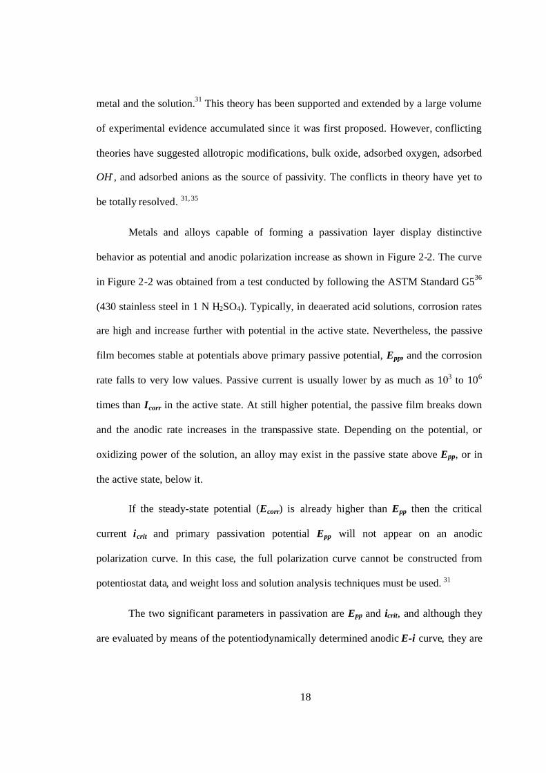
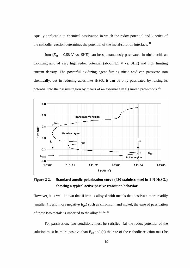
Metals and alloys capable of forming a passivation layer display distinctive
behavior as potential and anodic polarization increase as shown in Figure 2-2. The curve
in Figure 2-2 was obtained from a test conducted by following the ASTM Standard G536
(430 stainless steel in 1 N H2SO4). Typically, in deaerated acid solutions, corrosion rates
are high and increase further with potential in the active state. Nevertheless, the passive
film becomes stable at potentials above primary passive potential, Epp, and the corrosion
rate falls to very low values. Passive current is usually lower by as much as 103 to 106
times than Icorr in the active state. At still higher potential, the passive film breaks down
and the anodic rate increases in the transpassive state. Depending on the potential, or
oxidizing power of the solution, an alloy may exist in the passive state above Epp, or in
the active state, below it.
If the steady-state potential (Ecorr) is already higher than Epp then the critical
current icrit and primary passivation potential Epp will not appear on an anodic
polarization curve. In this case, the full polarization curve cannot be constructed from
potentiostat data, and weight loss and solution analysis techniques must be used. 31
The two significant parameters in passivation are Epp and icrit, and although they
are evaluated by means of the potentiodynamically determined anodic E-i curve, they are
19
equally applicable to chemical passivation in which the redox potential and kinetics of
the cathodic reaction determines the potential of the metal/solution interface. 31
Iron (Epp = 0.58 V vs. SHE) can be spontaneously passivated in nitric acid, an
oxidizing acid of very high redox potential (about 1.1 V vs. SHE) and high limiting
current density. The powerful oxidizing agent fuming nitric acid can passivate iron
chemically, but in reducing acids like H2SO4 it can be only passivated by raising its
potential into the passive region by means of an external e.m.f. (anodic protection). 35
-0.8
-0.3
0.3
0.8
1.3
1.8
1.E+00 1.E+01 1.E+02 1.E+03 1.E+04 1.E+05
i (A/cm2)
Evs
SC
E
Passive region
Active regionEcorr
ip
Ebd
Transpassive region
Epp
icrit
Figure 2-2. Standard anodic polarization curve (430 stainless steel in 1 N H2SO4)
showing a typical active passive transition behavior.
However, it is well known that if iron is alloyed with metals that passivate more readily
(smaller icrit and more negative Epp) such as chromium and nickel, the ease of passivation
of these two metals is imparted to the alloy.31, 32, 35
For passivation, two conditions must be satisfied; (a) the redox potential of the
solution must be more positive than Epp and (b) the rate of the cathodic reaction must be
20
greater than icrit. 31, 35 Figure 2-3 shows diagrammatically how a typical active-passive
metal will corrode when the reduction reaction is spontaneously held at different potential
values (cases a, b and c). Case a) Curve h-i may be a typical reduction reaction case for
an acid solution-stainless steel system at oxygen free conditions (that means hydrogen
reduction, equation (2-2)). In this case, neither of the two criteria for passivation is
satisfied and the metal is active, corroding at high rate. Case b) The presence of a small
amount of oxygen in the solution which would increase the potential for the interface
metal/solution (curve d-e-f-g) could worsen the situation, since iL<icrit. Case c) If the
oxidizing power of the solution is increased (large supply of oxygen is enough for some
systems), complete passivation could result (curve a-b-c). 31
However, additions of dissolved oxygen cannot passivate the ferritic stainless
steels in acid solutions because iL for oxygen reduction is insufficiently large. However,
passivation could be achieved if another oxidant (HNO3, Fe3+, Cu2+) with a high limiting
current density is present in the acid. 35
Figure 2-4 presents again previous cases a and c; but now a comparison is made
between the theoretical scheme and the corresponding experimentally-determined curve.
Suppose the cathodic curve intersects the anodic curve in the active region, as in Figure
2-4a. In this case, the full active-passive transition will be experimentally shown, as
represented in Figure 2-4b. This is the typical case for 430 stainless steel in 1 N H2SO4 as
shown in Figure 2-2. As mentioned before, if the cathodic curve intersects the anodic
curve in the passive region only, as in Figure 2-4c the material will passivate
spontaneously. Experimentally, the anodic curve for a specimen that has already been

21
spontaneously passivated does not exhibit the peak-shape active to passive transition, as
shown in Figure 2-4d.
Figure 2-3. Schematic of active-passive transition. Potentiostatic anodic curve
“jklm”; hydrogen evolution reaction, curve “hi”; low concentration of
dissolved oxygen, curve “defg”; high concentration of dissolved
oxygen, curve “abc”.31
Both oxidizer concentration and solution velocity have similar effects on the
corrosion rate of an active-passive alloy. In particular, if the passive state is stable, and
corrosion rate falls to low values when the rate of cathodic reduction is made sufficiently

22
high, the criterion for passivation is in place, i.e., the passive rate is stable when the rate
(current density) for cathodic reaction, is greater than the critical anodic current density,
icrit. Based on this criterion, alloys having lower icrit and more active Epp are more easily
passivated. 31
Higher acidities and higher temperatures generally reduce the passive potential
range and increase current densities and corrosion rates at all potentials. Usually, alloying
the metal with a noble metal that has a higher exchange current density than that of the
metal to be passivated will promote passivation even in a reducing acid. This was
achieved first by Tomashov who alloyed Fe-18Cr-8Ni stainless steel with Pt, Pd or Cu. 35
Potentiodynamic techniques require that the corrosion potential be constant
during the measurement, which in practice, requires the use of very slow scan rates.
Otherwise, the actual overpotential for any given current measurement would be
erroneously estimated. That is, the potentiodynamic scan must be run slowly enough to
ensure steady-state behavior.31 Mansfeld37 has shown potentiodynamic polarization data
for AISI 430 stainless steel (without Ni) which are dependant on scan rate only in the
passive range and not in the active range.

23
Figure 2-4. Theoretical and actual potentiodynamic plots of active passive metals
(Princeton Applied Research, Application Note, Basics of corrosion
measurements, 1982).
Passive film
The study of corrosion also includes the study of the nature of corrosion products
and of their influence on the reaction rate. These may be formed naturally by reacting
with their environment or as a result of some intentional pretreatment process to enhance

24
the protective properties of films by modifying the nature of existing films. These
corrosion products frequently form a kinetic barrier that isolates the metal from its
environment and thus controls the rate of the reaction. Thickness alone does not provide a
criterion of protection; actually the kinetics of attack is related to a variety of other
factors such a composition, structure, adhesion to substrate, cohesion, mechanical
properties, etc. of the film or scale of reaction products. 35
“A lack of fundamental understanding of passive film properties has delayedthe control and prevention of localized forms of corrosion that result from breakdownof the passive film. The most conveniently determined film properties involvechemical and electrochemical measurements, which have been difficult to interpretobjectively. Unfortunately, ex-situ examinations for direct determination of structureand composition (e.g., in vacuum by electron spectroscopy) are likely to change thefilm structure by dehydration and precipitation of new phases on the surface”. 31
Uhlig and co-workers have emphasized the role of chemisorbed oxygen in
establishing passivity. They suggested that adsorbed films provide a kinetic limitation by
reducing the exchange current density, io, for the anodic reaction instead of acting as a
barrier to dissolution reaction. 31 An initial chemisorbed state on Fe, Cr and Ni has been
postulated by the same authors in which the adsorbed oxygen is abstracted from the water
molecules. A different phase oxide or other film substance emerges at thicknesses within
1-4 nm with a corresponding increase in the anodic potential. Increase in the anodic
potential may lead to the following sequence:35
oxidephasemultilayermonolayer
2 .)( MOOHMOHMM
“Other theories consider that chemisorption of oxygen is favored by thepresence of uncoupled d-electrons in the transition metals. In Fe-Cr alloys, chromiumacts as an acceptor for uncoupled d electrons from iron. When alloyed Cr is less than12%, uncoupled d electron vacancies in Cr are filled from the excess Fe, and thealloys act like unalloyed iron, which is nonpassive in deaerated dilute acid solutions.

25
Above 12% Cr the alloys are passive in such solutions, presumably becauseuncoupled d electrons are available to promote adsorption. During film thickening,metal cations are assumed to migrate into the film from the underlying metal, as wellas protons (H+ ions) from the solution”. 31
Such films usually have low ionic conductivities that restrict cation transport
through the film. Shreir35 proposed that the electronic semiconduction, however, permits
other electrode processes (oxidation of H2O to O2) to take place at the surface without
further significant film growth. However according to Jones the passive film can begin to
grow in thickness once the metal achieves a stable passive potential region above Epp, as
evidenced by decrease in ipass with time, t, asymptotically (Figure 2-5). However, Jones
emphasizes that no true steady state is ever attained since the passive current density still
falls with time, but at continuously decreasing rate, as shown in Figure 2-6.31
Figure 2-5. Decay of passive corrosion rate measured by potentiostatic current. 31

26
Figure 2-6. Log-log plot of data from Figure 2-5 at extended times. 31
Maintenance and breakdown of passivity
Once established, a passivated state can often be maintained by conditions much
less demanding than those required to produce it. Any environment that maintains the
potential of the surface above Epp while supplying the very small passive current assures
passivity. The very large current icrit demand just before passivation is not required. The
passive potential may likewise be maintained by the presence in the solution next to the
passive surface of any oxidizing agent that provides the cathodic reaction.
“Shreir has mentioned that “stainless steels are easily maintained passivebecause both their air-formed oxide films and anodically formed oxide (containing Cr(III)) are ’stronger’ and stable at more negative potentials than the correspondingfilms on iron.” 35
Any factor that produces partial or complete removal of the passivating film can
cause partial or complete breakdown of passivity, and the corrosion rate can be

27
significantly accelerated. Such removal can be provided by a different degradation
mechanisms namely electrochemical reduction or oxidation, undermining by attack on
the underlying metal at film imperfections, or at mechanical disruption. The breakdown
of the passive film due to flows containing solid particles like sand falls into the latter
classification.
Since the passivating oxide films usually consist of brittle material, they are
subject to damage when a mechanical force is applied to them (through bending,
stretching, impact, and scratching, among others). When a passivated material is used to
reduce the corrosion rates in a given corrosive system where an inevitable mechanical
damage will occur, the material can be relied on only under conditions for which it is
chemically or electrochemically self-healing. In general, the uses of passive metals such
as stainless steel are under conditions providing self-healing by chemical processes.
However, many practical cases exist where stainless steel passivated by special
treatments (nitric acid or chromate treatment instead of self-healing) is little better than
the same material with a natural air-formed oxide film. These treatments are commonly
applied when the service condition of the stainless steel involves a corrosive environment
that does not promote self-healing, and slight mechanical damage soon leads to partial or
complete depassivation. 35
Stainless Steel
Alloying elements
Chromium plays a key role in forming the passive film. Other elements can
increase the effectiveness of chromium in forming or maintaining the film, but they

28
cannot, by themselves, create the corrosion resistant properties of stainless steel.31, 38
Protective films have been observed if more than about 10.5% Cr is present in the alloy,
but the film is fairly weak at this composition and provides only mild atmospheric
protection. Increasing the chromium content to higher levels (17 to 20% in austenitic
stainless steels, or 26% in ferritic stainless steels), greatly increases the stability of the
passive film. However, greater amounts of chromium may adversely affect mechanical
properties.38
Figure 2-7 shows anodic polarization for alloys of approximately constant Ni and
variable Cr content in hot sulfuric acid. It should be note that below 12% Cr the passive
potential region is considerably restricted. 31
With chromium levels of about 13% and relatively high carbon levels, it is
possible to obtain austenite at elevated temperatures. By accelerated cooling, the
austenite transforms to martensite. Similar to carbon steels and low-alloy steels, this
strong martensite can be tempered to a favorable combination of high strength and
adequate toughness.33 This is the case of the conventional 13Cr used in the oil industry
for well completion. It has shown excellent CO2 corrosion resistance; however its
protective properties against corrosion are considerably diminished if H2S is present in
the flow.
In recent years, nitrogen, nickel, and molybdenum additions at somewhat lower
carbon levels have produced martensitic stainless steels of improved toughness and
corrosion resistance.

29
Figure 2-7. Effect of chromium content on anodic polarization of Fe-Ni alloys
Flow velocity effects
According to the nature and intensity of the flow parameters like wall geometry,
flow environments lead to corrosion types caused predominantly by either mass transport
or wear. Lotz and Heitz39 made an attempt to classify the various types of flow-dependent
corrosion in relation to existing standards for corrosion and wear.
Fluids acting on the corrosion system material/medium have mainly two effects:
a) They influence the transport of reactants and products by convection (mass transfer by
convective diffusion), and b) They create shear stresses and pressure fluctuations on the
surfaces, and cause wear. The authors distinguish three broad areas of flow-dependent
corrosion based on these effects.

30
1. Absence of forced convection (but natural convection is present).
When no flow is produced, forced convective mass transfer is not present. As a
result enrichment of hydrogen ions by hydrolysis of anodic products and the enrichment
of chloride ions (as a result of migration in the electric field) favor forms of corrosion like
pitting and crevice corrosion. Absence of some type of protective layers typical of mass
transfer processes is also observed in stagnant conditions.
2. Corrosion influenced by convective mass transfer
In this case mechanical flow effects (shear stresses) are negligible. More likely
the corrosion is mainly caused by the transport of reactants and reaction products. If the
process is material transport-controlled the flow-dependency of the corrosion system is
greater than if it is predominantly reaction-controlled.
3. Corrosion influenced by mechanical flow effects
For those conditions where mechanical forces are significant at the interface
metal/fluid, erosion and cavitation corrosion occur. A sudden increment in the corrosion
rates, for flow rates above critical values, usually indicates these types of material
degradation. Hydrodynamic parameters as well as the corrosion system define the critical
flow rate ucrit for the appearance of erosion-corrosion. Therefore, the critical flow value
may change with changes in the fluid flow parameters and changes in the corrosive
environment as well. The fluids also may contain solids or gas bubbles, and very different
metal removal rates may be obtained as a result of differing mechanical effects even for
identical flow rates.
Corrosion failures in the oil industry are normally associated with disturbed flow
conditions as a result of weld beads, preexisting pits, bends, flanges, valves, tubing

31
connections, etc. Due to the complex hydrodynamics of these conditions, attempts at
relating flow effects to steel corrosion have been only partially successful. Estimates of
the effects of the wall shear stress and steady state mass transfer in corrosion testing is
required for estimation of steel corrosion under disturbed flow conditions. The processes
that control corrosion and film formation occur in the turbulent boundary layer and
diffusion boundary layer. In this region, the chemical reactions occur as well as all
movement, to and from the pipe wall, of the chemical species involved in the corrosion
process. As a result, disturbances in the turbulent boundary layer, particularly within the
viscous region, affect the corrosion process.40
Flow pattern effects
A complex interaction of physical and chemical parameters is involved in the
effect of fluid flow on corrosion of steel in oil production. Water wetting the metallic
surface is one of the main requirements for any corrosion to occur. This is strongly
affected by the flow regime. Mass transfer and wall shear stress parameters governing
behavior in the water phase that contacts the pipe wall greatly control the effect of flow
on corrosion (flow accelerated corrosion).40
Flow accelerated corrosion has been defined as “corrosion resulting from the
effect of fluid turbulence due to flow of a fluid that does not contain solid particles.” 40
Flow turbulence occurring in most flows is responsible for accelerating the corrosion of
metal pipe in contact with a flowing electrolyte. These fluctuations increase the mobility
of the corrosive species to the metal surface as well as help to remove the products of the
corrosion reaction from the boundary layer in a more efficient manner. On the other hand,

32
for laminar flow, the effect of fluid flow is inconsequential. The physical structure of
turbulent flow is thus a primary consideration since in most oil and gas situations where
fluid flow accelerates corrosion, the flow is turbulent. 40
In general the wear caused by a flowing single-phase liquid on the surface of a
metal is small, since the wall shear stresses are small too. Significant wear damage may
appear in multi-phase flows, especially if solid particles are present in the flow causing
erosion.39
When both mechanical forces (wear) and material transport are acting together,
there are many processes involved and the interaction between those mechanisms plays a
key role in the understanding of the overall phenomenon. The surface layer may be
removed, leading to an intense local attack. Where the surface layer has been removed,
the material transport may determine the deterioration rate. More complex corrosion
mechanisms can be activated as corrosion cells between the bare surfaces (anode) and the
surfaces with an oxide film (cathode), and consequently a galvanic effect arises.
When solid particles are present in the fluid, erosion problems may arise. The
momentum of the particles carries them into contact with the metal surface. When the
impact kinetic energy is high enough, wear results. Additionally, solid particles entering
the boundary layer increase the turbulence intensity and the mass transfer may be
accelerated. However, particles that are less dense than the liquid may not involve any
additional material transport, since they do not penetrate the laminar boundary layer.39
In most cases, a relationship between the weight loss WL and the flow rate u can
be approximated with an exponential relation of the form WL ~ ua.

33
Usually the value of the exponent, a changes according to the mechanism
involved in the degradation process. For non-flow-dependent corrosion, a is equal to zero
(limiting phase boundary reaction).
Heitmann discussed this subject of erosion-corrosion in water-steam loops and
suggested that plain carbon steel corrodes at a higher rate with WL ~ u2 (erosion-
corrosion); and, low alloy steels corrode very slowly, with WL ~ u0.5 (transport-affected
corrosion). In the case of wear due to solid and liquid impingement, as well as erosion-
corrosion, exponents of 2 < a < 4 are commonly found. 39
It should be mentioned that the type of control of a corrosion process, by transport
alone, by mechanical means alone, or mixed means, depends not only on the
hydrodynamics but also on the corrosion system itself. The electrochemical or chemical
limitations and their influence on the formation and stability of surface layers are of
particular importance.
CO2 Corrosion Resistance of 13Cr Alloy
There have been several studies of the kinetics and mechanism of the cathodic
reaction in slightly acidic oxygen-free CO2-containing solutions of the type encountered
in oil and gas production, and several different reaction mechanisms have been proposed.
41-46 The majority of these studies have been in the pH range of 4 to 4.5, with the pH
controlled by the partial pressure of carbon dioxide. While there are still disagreements
about the precise mechanism, the involvement of potentially complex preceding or
subsequent chemical reactions is known to modify the electrochemical responses.

34
There have been many studies of the cathodic reaction mechanism and several
different processes and rate determining steps have been proposed. These include rate-
determining reduction of carbonic acid with subsequent reformation from the bicarbonate
and protons41 and rate limiting diffusion of bicarbonate.42 Even greater complication
would result from these mechanisms by adding the interaction of the solution with a
chromium rich layer.
The resistance of 13Cr stainless steels to uniform corrosion has been determined
by weight loss by several authors. Crolet and Bonis47 made corrosion rate measurements
after exposures of one month in laboratory autoclaves. The tests were conducted in highly
acidic, relatively concentrated brines, 30 g/L (0.5 M) NaCl, with CO2 pressure within the
range of 14 to 420 psi and at temperatures of 70 to 250oF (20 to 120oC). Despite these
severe conditions, the samples always remained passive or only very slightly active, and
the weight losses never exceeded 0.5 mpy (0.01 mm/y). Moreover the effect of flow was
not determined.
Cayard and Kane3 summarized the corrosion rate data of conventional 13Cr and
modified 13Cr from several authors. The data set represents a range of conditions with
respect to CO2, H2S, temperature and Cl-. The corrosion rates at low pH for conventional
13Cr were in general higher than the corrosion rates for modified 13Cr as expected.
However, above a pH of approximately 4.2, the corrosion rate remains quite low for both
alloys.
Many authors have investigated effects of flow velocity on corrosion behavior in
wet CO2 environments. Several of them used flow loops to establish the effect of the fluid

35
flow in the corrosion mechanism for corrosion resistant alloys (CRAs); also, comparisons
with carbon steel tested at similar conditions are available.
For the case of carbon steel, Denpo et al. showed that the corrosion rate of N80
steel obeys 0.62th-power law under turbulent conditions according to:48
398.062.0Re097.0 ScSh (2-13)
where Sh is the Sherwood number defined by
D
dkSh m (2-14)
where, km is the mass transfer coefficient, d is the diameter (characteristic length) and D
is diffusion coefficient of the specie in solution. The Reynolds number, Re, is defined by
dv
Re (2-15)
where, v is the fluid velocity, is the fluid density, is the fluid dynamic viscosity, and
the Schmidt number, and Sc is defined by
DSc
(2-16)
where, is the kinematic viscosity andD is the diffusion coefficient of the specie
in solution.
De Waard et al.41 showed that the flow dependence of the corrosion rate of carbon
steel is proportional to 0.8th- power law in turbulent flow.
30.080.0Re097.0 ScSh (2-17)

36
Therefore, the effect of fluid flow on corrosion rate could be formulated in the form of an
exponential law.
cb ScaSh Re (2-18)
where a, b, c are constant. However, the b value, which governs the flow dependence of
the corrosion rate, needs to be determined more precisely for carbon steels and low alloy
steels.48
According to Denpo, the corrosion rate of AISI 420 type (13Cr) steel obeys to a
0.5th- power law in a flow velocity range up to 3 m/s (9.84 ft/s), while at flow velocities
above 3 m/s the corrosion rate is constant. Hara et. al.48 found the CO2 corrosion rate of
AISI 420 type (13Cr) steel to be independent of flow velocity at 120 and 150oC. They
claim that even under flowing condition, the protective film is presumed to remain stable.
The flow dependence of corrosion rate for modified 13Cr steels and duplex stainless
steels still needs to be investigated.
Basic Erosion Concepts
To classify the wear on the basis of the fundamental mechanism that is operating
is a difficult task if more than one mechanism is operating at the same time. The
definition of the mechanism and the distinction between different mechanisms sometimes
are not well defined, thus, the semantic aspect further complicates attempts to classify the
phenomena. As a result, different classification schemes based on wear mechanisms have
been developed; however, no one scheme is universally accepted. Most of them have
reasonably similar features. Budinski reduces wear processes into four categories;
abrasion, erosion, adhesion, and surface fatigue as shown in Figure 2-8.49

37
Figure 2-8. Major categories of wear based on their fundamental mechanisms. 49
Solid particle erosion
The loss of material that results from repeated impacts of solid particles, carried
by a fluid, on the target surface material is called solid particle erosion (SPE). If hard
particles are entrained in a fluid flowing at any significant velocity, significant erosion
rates may arise. Fluid flow conditions affect particle acceleration and direction. When

38
particle concentration is very high, the wear phenomenon is called slurry erosion and is
generally treated as a different, though related, subject.
Ludema recently collected and analyzed a large number of analytical models of
the wear processes available in the literature50. His paper illustrated the lack of the ability
of the tribology field to develop a usable model for any wear process, sliding, abrasion, or
erosion. He used solid particle erosion to explain the problem. He reviewed 98
mathematical erosion models and discarded all but 28 of them because they were “not
amenable to conclusive scrutiny.” The 28 remaining equations have a total of 33
variables used by the various authors. No model used more than 7 of them. From 1 to 8
constants are in each model. There was no consistent pattern of use of the variables.
Some used the same variable in the numerator that others used in the denominator. None
of the models could accurately predict material loss rates.50
Because of the complexity and degree of controversy involved in the
modeling of solid particle erosion, a brief description of only the ductile and brittle
mechanism accepted by many authors is given below.
It is a common practice to classify materials as ductile or brittle, based on the
dependence of their erosion rate on , defined throughout virtually all erosion literature
as the angle between the incident particle direction and the tangent to the target material
surface. Commonly, some pure metals classified as ductile materials have a maximum
erosion rate at low angles of incidence (typically 15o to 30o), while ceramics (brittle
materials) present the maximum erosion rate at or near 90o. These cases are illustrated in
Figure 2-9. Intermediate cases between those examples exist and sometimes the same

39
material shows behavior that shifts from one extreme to the other, depending on erosion
conditions.49
Erosion of ductile materials
Hard angular particles impinging a smoother surface may cut the surface. The
theory of erosive cutting for ductile materials by Finnie (1978), distinguishes between
two types of cutting processes: (1) “The particle is stopped during the cutting action at
the depth for which its kinetic energy dissipates, or (2) The particle enters the ductile
surface and subsequently leaves it with some the remaining kinetic energy, together with
surface material.” 51
The maximum rate of material removal for ductile erosion is at a low angle of
impingement as shown in Figure 2-9. The pattern of the eroded surface often shows
evidence of material deformation in the form of particle tracks, ripples, or micro grooves
at low angles and impact craters at high angles. When the impinging particle impact
angles are 90 degrees (= 90o) or graze the surface (= 0o), the weight loss due to
ductile cutting action is negligible.
Erosion of brittle materials
Some authors have proposed that the erosive wear in brittle materials occurs when
the stress generated in the material by impacting high-velocity particles exceeds the
material’s maximum tensile strength, forming cracks on the surface. If the remaining
particle kinetic energy after the initial surface cracking is high enough, additional particle
penetration may occur. This suggested that the removal of material is dependent on the
particle velocity (v). The erosion resistance of brittle materials is nearly proportional to

40
the strain energy of the material at its tensile strength. As mentioned before, brittle
erosion presents a maximum material loss for particles striking the surface at right angles
( = 90o) as illustrated in Figure 2-9. The mechanism of material loss is through
microfracturing and removal of fractured segments by subsequent impacts.51
Figure 2-9. Schematic of the effect of the impingement angle on erosion rate of
ductile and brittle materials
Variables influencing erosion
The variables influencing pure erosion can be classified as one of three types:
impingement variables describing the particle flow, particle variables, and material
variables. The most important impingement variables are particle impact velocity (v),

41
angle of incidence (), and particle flux (particle concentration). Particle variables
include particle shape, size, hardness, and friability (ease of fracture). Material variables
include all the material properties, such as hardness, work hardening behavior, and
microstructure.49
Particle Impact Velocity: Since the kinetic energies of particles moving at high
velocities are also high, they have more potential to degrade the surface than particles
moving at lesser velocities. Hence, particle velocity is directly related to the erosion rate.
Previous work conducted with steel to determine the volume loss per impact due to
changes in velocity, reported that erosion was proportional to a simple power of
velocity.49 That is
nbvE (2.15)
where v is the velocity of erodent and n is a constant. It can be said that the value of n
usually falls in the range of 2 to 2.5 for metals and 2.5 to 3 for ceramics, even though
authors have reported values outside these ranges.
Impact Angle: As mentioned before, incidence angle or impact angle, of the
particle onto the surface of the target is another parameter which greatly influences
erosion. The influence of impact angle can also help in distinguishing between ductile
and brittle materials. For ductile materials the erosion loss is maximum at lower angles of
incidence (around 15-30o) whereas in brittle materials the erosion loss is maximum at
normal incidence around 900.
Particle flux (particle concentration): Previous research at the Erosion/Corrosion
Research Center (E/CRC) at The University of Tulsa has shown the linear proportionality
42
of erosion rates with sand concentration so long as concentrations remain low (£ 2% by
weight in liquid). Kohley and Heitz52 have reported the same behavior for 13Cr alloys.
Particle shape: The shape of the particle is also very important in predicting the
erosion rate due to particle impact. The contact area between the particle and the metal
surface during an impact is determined by the particle shape. More severe erosion
damage is generally associated with angular particles for both ductile and brittle
materials.49
Particle Size: Most theories predict no effect of particle size for metals, although
it is often observed that erosion rate increases strongly with particle size, at least up to
about 100 microns.49, 50
Particle hardness, particle friability and material variables are important variables
to be considered in erosion modeling. In 1995, Levy50 made an effort to combine all his
experimental and theoretical work and correlating it with other theories in a single
volume. In this book, the effect of the erodent characteristics as well as the material
properties of the target are well addressed but the trends very much vary with each target
material-erodent system.
Erosion-Corrosion
Lotz and Heitz39 combined corrosion standard, DIN 50900 with the wear standard
DIN 50320 to make a classification of the types of mechanical/chemical attack. They
claim that in addition to thermal/chemical attack, there is mechanical/chemical attack that
may be classified as follows:

43
Wear at the phase boundary. Stress and fatigue corrosion and forms of mechanical/chemical/thermal
attack in the material. Transport-determined corrosion in the liquid medium (hydromechanical
effects).
In a pure wear situation, whether the weight loss comes from mechanical removal
of the passive layer or removal of the base material itself would not significantly affect
the final erosion rates, whereas under corrosive conditions, damage in the surface layer
and a competition between layer removals versus layer self-healing may signify huge
differences in final weight losses. The term “erosion-corrosion” is defined in DIN 50900
as the “combination of the mechanical removal of a surface (erosion) and corrosion,
where the corrosion is initiated by the destruction of protective layers as a result of
erosion”. This standard only accounts for the mechanical damage caused by wear. The
stimulation of a corrosion process by a fluid-mechanical component is generally also
referred to as erosion-corrosion.39
The research presented in this dissertation deals with the erosion-corrosion of a
13Cr as a consequence of having mechanical wear due to the presence of sand particles
suspended in a CO2 saturated brine fluid. The mechanical wear will be occurring in the
protective layer as an initial stage and if erosivity conditions are severe enough, base
metal also can be removed. Therefore in this research, erosion-corrosion can be
understood as the combination of erosion of the protective layer (and perhaps also base
metal) and corrosion of the underlying metal, which is a common cause of failure in
oilfield equipment.
Some people use the term impingement to refer to a phenomenon similar to
erosion-corrosion but even more localized. Impingement attack occurs when a particle

44
stream impinges upon a metal surface and breaks down protective films in very small
areas (solid particles suspended in a fluid and impacting the inner metallic surface of a
pipeline). The resulting attack is in the form of pits that are characteristically elongated
and undercut in the downstream end. Impingement often results from turbulence
surrounding irregularities in the metal surface. It is particularly a problem in copper and
copper-based alloys.32
Carbon steel and low alloy steels are particularly susceptible in environments
which form scales, such as iron carbonate, that are easily removed. The attack normally
occurs only at certain areas, such as changes of sections or connections where there is
turbulence from flow or at bends and elbows.32 The austenitic stainless steels have high
resistance to both erosion-corrosion and impingement type attack; however, erosion of
the passive film can lead to some acceleration of attack. 31, 32, 38 Under severe conditions
erosion-corrosion of 13Cr alloy has been reported.52, 53
In general, it can be said that corrosion of a metal or alloy can be accelerated
when there is an abrasive removal of the protective oxide layer. The important issue here
would be how significant is the acceleration of the damage. Some authors think this form
of attack is especially significant when the thickness of the oxide layer is an important
factor in determining corrosion resistance. 38
ASTM proposes a “Standard Guide for Determining Synergism between Wear
and Corrosion.”54 The guide provides a means for computing the increased wear loss rate
attributed to synergism or interaction that may occur in a system when both wear and
corrosion processes coexist. The standard proposes four types of tests to obtain values
for: total material loss, T which accounts for pure wear and pure corrosion as well as the

45
synergistic term;. Material loss due to pure erosion, Wo; Material loss due to pure
corrosion, Co; Penetration rate due to corrosion under conditions of corrosion wear Cw.
This can be measured by electrochemical means and is usually higher than Co because of
mechanical wear interaction.
Finally, the standard proposes some calculations to determine S’ as the increase of
mechanical wear due to corrosion, S’’ as the increase of corrosion due to mechanical
wear, and S as the total synergistic effect (S = S’ + S’’). Similar approaches have been
employed by other authors.55, 56 In any case, the analysis of erosion-corrosion problems is
a difficult task. Many variables are involved. Isolating and classifying the effect of each
of them would be tedious work, and even more difficult would be determining the
relationships between the behaviors of the each variables and their integrated effect in the
mass loss rate.
Material selection is also an important consideration for erosion-corrosion
resistance. Alloy hardness has also been shown to be a factor. Generally, soft alloys are
more susceptible to erosion-corrosion than their harder counterparts; but the relative
hardness properties of the alloy can be misleading because the hardening process itself
affects resistance to erosion-corrosion.38
Some researchers38, 52, 56 have used electrochemical techniques to determine the
effects of concentration of sand and flow velocity in the erosion-corrosion of some alloys.
Figure 2-10 shows a schematic of polarization plots for type 316 stainless steel that was
exposed to sand slurries at different sand concentrations and impeller velocities. Notice
how the anodic current density increases as percent solids and speed increase. This is
pointed out by the author as an indication that more of the passive film is removed

46
because of the higher frequency of particle impacts. The oxide film on the stainless steel
is apparently adherent and fast forming. The author also claims that the polarization
curves and corrosion rates of low-alloy steels were not affected to any extent because
they freely corrode and do not form tightly adhering passive films. 38
-0.800
-0.700
-0.600
-0.500
-0.400
-0.300
-0.200
1.E-07 1.E-06 1.E-05 1.E-04 1.E-03 1.E-02
Log (current density)
Po
ten
tial
0% solids 2% solids 30% solids
Figure 2-10. Schematic of polarization curves for type 316 stainless steel showing
the effect of percent solids sand slurry.38
13Cr Alloy and Erosion-Corrosion
Kohley and Heitz52 also determined the mass loss rates of 13Cr in oil formation
water containing particles, using a loop with a constricted pipe as a test section. Figure 2-
11 shows the influence of flow velocity (Re number) on the corrosion rate along the pipe
length in front and behind the constriction in the pipe. On the x-axis, a normalized pipe

47
length x/D, with D= 50 mm, is plotted. The flow velocity is varied from 1 to 5.7 m/s in
the 50 mm diameter tube. At the entrance of the pipe constriction, the mass loss rates go
through a maximum. For example, the mass loss rate upstream of the constriction (5.7
m/s) exceeds 20 mm/year. At x/D=0.5 just downstream of the pipe expansion, a
minimum occurs, followed by a second maximum.
Figure 2-11. Plot of the mass loss rate vs. normalized distance from the pipe
expansion at different flow rates. (60oC, 3 bar CO2 and 1000 ppm of
sand (Re number 5.7 105 correspond to a flow velocity of 5.7 m/s). 52
The penetration rate at the maximum downstream of the constriction was found to
increase according to the power of 1.85 of the flow speed (WL ~ u1.85). The authors
suggested that the first maximum in Figure 2-11 could be attributed mainly to abrasive
wear and the second maximum to erosion-corrosion. They found at the inlet edge of the

48
constriction, the removal rate was far higher than the electrochemical corrosion rate,
which implies a marked mechanical abrasion of the base material.52
In sand-free flow, no differences between rates along the pipe length can be
observed. Figure 2-12 presents the dependence of the mass loss rate on the sand
concentration. At x/D = 2.5 (second max), a rise in the sand concentration is responsible
for a significant increment in the erosion-corrosion rate.
Figure 2-12. Influence of various sand concentrations on the mass loss rate along
the pipe length at a flow rate of 3.5 m/s. 52
If the mass loss rates at the point of maximum corrosion are plotted against the sand
concentration, a straight line is obtained which means that the erosion-corrosion rate is
directly proportional to the number of particles hitting the metal surface. The findings
were explained by the authors as a breakdown in passivity of 13Cr in sand-containing
formation water due to particle impacts on the metal surface. They claim high kinetic

49
energy particles not only destroy the passive layer, but also the base material, and
mechanical wear is the result. This holds for the entrance region of the constriction of the
segmented tube. Medium energy particles only destroy that passive layer, and if the
kinetics of the healing process is slower than the particle impact kinetics, erosion-
corrosion accelerates. The intensity of the corrosion is therefore a function of the
hydrodynamics of the flow. As a result, the area of maximum erosion-corrosion
downstream of the orifice can be explained as the region in which reattachment of the
flow with high particle impact frequency occurs. 52
Birchenough et al.53 studied the erosion-corrosion phenomena of 13Cr under a
very broad range of flow conditions for an expansion and for an elbow geometry in flows
containing sand. Figure 2-13 shows the results obtained by Birchenough53 et al. (1996).
Figure 2-13. Thickness loss versus time for a 13Cr alloy exposed to CO2 saturated
brine containing sand particles. 53

50
They claim the 13Cr was found to be resistant to corrosion under sand free flow
conditions. Sand was then added after an initial sand-free period according to the history
shown in Figure 2-13. Initially, erosion at a rate consistent with the pure erosion tests was
observed. After approximately 1.5 microns of material had been removed, the removal
rate increased to a value approaching 6 m/d, which was found to persist even though
sand concentration was falling. The authors believed that the sudden change in material
loss rate after approximately 1.5 microns of material loss corresponds to corrosion of the
bare metal following erosion of an oxide film previously established. Finally, they
claimed that high corrosion rates could be sustained after removal of the 1.5 microns of
oxide layer, even when sand is no longer present in the flow since the system is not able
to repassivate in an oxygen free environment. 53
In recent years, research has been conducted at The University of Tulsa, on
erosion-corrosion of 13Cr. In the past, several measurement techniques have been used to
help better understand the different mechanisms involved in the degradation of 13Cr
when exposed to a CO2 corrosive environment containing sand particles. Weight loss,
thickness loss, linear polarization resistance (LPR), and potentiodynamic sweeps were
some of the techniques used. Tests were conducted under several flow conditions. Sand
effect results in single phase liquid flow as well as two phase (gas-liquid) flows, and the
effect of temperature were also addressed. The main findings in this area are highlighted
below.
In general, for both single-phase flow and multiphase flow conditions tested, the
erosion-corrosion penetration rates of 13Cr were higher than those of pure erosion. Both

51
sets of tests were conducted in an elbow geometry where direct impingement is expected.
However, hydrodynamic conditions as well as sand concentrations for both conditions
were quite different and should be considered when trying to draw conclusions from
these results.
Single phase liquid flow loop testing (high sand rates)
Rincon et al.57 and Chen et al.58 conducted single phase liquid tests for erosion-
corrosion of 13Cr alloy at 76, 150 and 200oF. In order to be able to measure some weight
loss in a reasonable period of time, tests were conducted at the maximum liquid velocity
of the miniloop, namely 15 ft/s. However, extremely high concentrations of sand were
needed to create significant weight losses in 13Cr samples in about 7 days. The sand
concentration used was 2% by liquid weight or more (>3,447 lb/day), which might be
much higher than those typical experienced in field conditions.
At 76oF, penetration rates due to erosion-corrosion were found to be from two to
three times higher than penetration rates for pure erosion.57 At higher temperatures (150
and 200oF) the factor increased to values approximately between 4 and 6,58 as can be seen
in Figure 2-14. A synergistic effect where erosion-corrosion rates were higher than the
sum of the penetration rates due to the erosion degradation and corrosion degradation
acting alone over the metallic surface was also evidenced. However, if sand is completely
removed from the system, the oxide layer has been proven to rebuild and provide a
corrosion protection level similar to the protection afforded originally when no sand was
in the system.

52
0
2
4
6
8
10
12
14
16
18
20
Temperature
Pene
tra
tion
rate
(mpy
)fr
om
wei
ghtl
oss
Erosion (mpy) 1.3 2.2 3.6
Ero-Corr (mpy) 4.5 15.3 18.5
(E-C)/E 3.5 7.0 5.1
76 °F 150 °F 200 °F
Figure 2-14. Comparison of penetration rates for pure erosion and erosion-
corrosion at different temperatures by the weight-loss method (single
phase liquid flow, Vl =15 ft/s). 58
Multiphase flow loop testing (high sand rates)
Rincon et al.57 also conducted erosion-corrosion tests for 13Cr alloy under
multiphase flow conditions. The multiphase flow facilities allowed increasing the flow
velocity and reducing the sand rates to more reasonable values. Flow conditions tested
were Vsg = 97 ft/s and Vsl = 0.2 ft/s with an annular flow pattern. The average sand
concentration was 2% by liquid weight representing about 48 lb/day of sand at tested
conditions. The penetration rates for erosion-corrosion were also found to be higher than
those observed for pure erosion tests, again by a factor of 2 to 3 as seen in Figure 2-15.
If the removal rate of the passive film is greater than the formation rate of the
passive film, then an accelerated corrosion process takes place. In most cases, there is

53
likely a competition between the protective film removal due to mechanical erosion and
the protective film healing. If erosivity conditions are severe enough, base metal can also
be removed by the mechanical erosion component. The mechanistic model of this
competition may depend on the concentration and distribution of sand as well as the flow
pattern and fluid flow velocities, geometry and environmental factors. The erosion-
corrosion behavior appears to be a function of both erosivity and environmental
conditions.
0
20
40
60
80
100
120
140
160
180
200
Pe
ne
tra
tio
nra
te(m
py
)(w
eig
ht
los
s)
Erosion 23 45 40 37 60 41
Ero-Corr 105 111 81 149 178 125
1 2 3 4 5 Avg.
Figure 2-15. Penetration rates for pure erosion and erosion-corrosion tests of 13Cr
in multiphase flow conditions (Vsg = 97 ft/s, Vsl = 0.2 ft/s). 57
Figure 2-14 and Figure 2-15 indicate that, in general, the erosion-corrosion
penetration rates were 2 to 3 times higher than the pure erosion rates for single-phase

54
flow as well as for multi-phase flow at room temperature. For higher temperatures, this
factor was even larger.
Over the same testing period that the erosion and erosion-corrosion tests were
conducted (6 hours) for multiphase flow conditions, the pure corrosion penetration rate
(without sand) would be so small that it would not be measurable with weight loss
techniques. Longer tests were needed to obtained measurable mass loss values for pure
corrosion conditions (without sand). A longer, (168 hours) pure corrosion test (included
in Figure 2-16) was performed and the corrosion rate was found to be about 2.3 mpy.
That corrosion rate is higher than the corrosion rate obtained for single-phase (below 1
mpy) conducted at lower velocities. 59
2.3 6.1 4.9
41
125
0102030405060708090
100110120130
Pen
etra
tion
Rat
e(m
py)
(wei
gh
tlos
s)
Corrosion EstimatedCorrosion 1
EstimatedCorrosion 2
Erosion (Avg.) Eros-Corr(Avg.)
Type of Test
Figure 2-16. Comparison among penetration rates for pure Corrosion, pure
Erosion and Erosion-Corrosion processes (Vsg= 97 ft/s, Vsl= 0.2 ft/s). 59
Also, a long test was designed to estimate the mass loss of 13Cr due to the sand-
free CO2 environment after being previously exposed to sand impingement for a period

55
of time. Two tests were conducted at these conditions. For the first 6 hours of the test,
erosion-corrosion conditions (2% sand + CO2) in multiphase flow were used (i.e., CO2
and sand acting together on the 13Cr surface). Later, all the sand was flushed out of the
loop and the 13Cr specimen was exposed to a sand-free CO2 flow for about 160 hours
more. Two aspects can be highlighted from results obtained from these two segments of
the tests.
The penetration rate obtained by dividing the total mass loss by the total test time
(166 hours) was quite low (about 10 mpy) compared to the average obtained for 6 hours
erosion-corrosion tests (125 mpy) shown in Figure 2-15. This suggests that the high
corrosion rates are not sustainable once the flow is sand-free, because the oxide layer
rebuilds. Assuming that the mass loss for the first 6 hours was similar to the average
obtained for 6-hour erosion-corrosion tests (125 mpy) shown in Figure 2-15, a corrosion
component for the sand-free condition can be estimated. To do this, the average of the
mass loss for erosion-corrosion tests shown in Figure 2-15 was subtracted from the total
mass loss measured for the two long tests. For calculating the pure corrosion penetration
rate, 160 sand-free hours were considered instead of the total testing time (166 hours).
The calculated penetration rates are shown in Figure 2-16. It should be mentioned that
some traces of sand could have been present for the remaining 160 hours at the presumed
sand-free condition. As a consequence, the estimated corrosion rates for these two tests
(6.1 and 4.9 mpy), shown in Figure 2-16, are a little higher than the strictly pure
corrosion test result (2.3 mpy). However, this small difference does not alter the
conclusions drawn here.

56
Figure 2-16 summarizes the averages of penetration rates for erosion-corrosion
tests and for erosion tests as shown in Figure 2-15 plus the pure corrosion test results and
the estimates of the corrosion component for the two long tests as explained in the
previous paragraph. Notice, the erosion-corrosion rate was higher than each of the
erosion and corrosion processes appraised separately. Furthermore, the erosion-corrosion
rate was higher than the sum of the erosion and corrosion components appraised
separately, e.g., 125 mpy >> 41 mpy + 6 mpy = 47 mpy (using 6 mpy for the pure
corrosion rate which is the worst case scenario).
These results suggest that the 13Cr specimen does not return to a completely
passivated state as long as the system is sufficiently erosive and as a result, a synergistic
effect between erosion and corrosion is exhibited.

57
60, 61,62,63,64
CHAPTER 1 ....................................................................................................................................1
INTRODUCTION .............................................................................................................................1
CHAPTER 2 ....................................................................................................................................5
BACKGROUND AND LITERATURE REVIEW..............................................................................5
Basic Corrosion Concepts .......................................................................................................5
Concept and Forms of Corrosion ............................................................................................................5
Review of the Electrochemical Basis of Corrosion ................................ .................................7
Theory behind Polarization measurements.............................................................................................8
Linear Polarization Resistance .............................................................................................................. 11
Potentiodynamic Polarization and Tafel Constants ............................................................................. 16
Active Passive Metal Behavior ..............................................................................................17
Passive film............................................................................................................................................. 23
Maintenance and Breakdown of Passivity............................................................................................26
Stainless Steel ................................ ................................................................ ........................27
Alloying elements................................................................................................................................... 27
Flow Velocity Effects ............................................................................................................................29
Flow Pattern Effects ..............................................................................................................31
CO2 Corrosion Resistance of 13Cr Alloy ..............................................................................33
Basic Erosion Concepts.........................................................................................................36
Solid Particle Erosion.............................................................................................................................37
Erosion of Ductile Materials.................................................................................................................. 39
Erosion of Brittle Materials ...................................................................................................................39
Variables Influencing Erosion............................................................................................................... 40
Erosion-Corrosion................................ ................................................................ .................42
13Cr Alloy and Erosion-Corrosion.......................................................................................46
Single phase liquid flow loop testing (high sand rates) ....................................................................... 51
Multiphase flow loop testing (high sand rates) ....................................................................................52
REFERENCES ................................................................................................................................59
FIGURE 2-1. CORROSION PROCESS SHOWING ANODIC AND CATHODIC CURRENT COMPONENTS.33 ...........9
58
FIGURE 2-2. STANDARD ANODIC POLARIZATION CURVE (430 STAINLESS STEEL IN 1 N H2SO4) SHOWING
A TYPICAL ACTIVE PASSIVE TRANSITION BEHAVIOR................................................................. .............19
FIGURE 2-3. SCHEMATIC OF ACTIVE-PASSIVE TRANSITION . POTENTIOSTATIC ANODIC CURVE “JKLM”;
HYDROGEN EVOLUTION REACTION, CURVE “HI”; LOW CONCENTRATION OF DISSOLVED OXYGEN, CURVE
“DEFG”; HIGH CONCENTRATION OF DISSOLVED OXYGEN, CURVE “ABC”...............................................21
FIGURE 2-4. THEORETICAL AND ACTUAL POTENTIODYNAMIC PLOTS OF ACTIVE PASSIVE METALS........23
FIGURE 2-5. DECAY OF PASSIVE CORROSION RATE MEASURED BY POTENTIOSTATIC CURRENT. 31 .............25
FIGURE 2-6. LOG-LOG PLOT OF DATA FROM FIGURE II-5 AT EXTENDED TIMES. 31 .................................26
FIGURE 2-7. EFFECT OF CHROMIUM CONTENT ON ANODIC POLARIZATION OF FE-NI ALLOYS .....................29
FIGURE 2-8. MAJOR CATEGORIES OF WEAR BASED ON THEIR FUNDAMENTAL MECHANISMS. 49 .............37
FIGURE 2-9. SCHEMATIC OF THE EFFECT OF THE IMPINGEMENT ANGLE ON EROSION RATE OF DUCTILE
AND BRITTLE MATERIALS .....................................................................................................................40
FIGURE 2-10. SCHEMATIC OF POLARIZATION CURVES FOR TYPE 316 STAINLESS STEEL SHOWING THE
EFFECT OF PERCENT SOLIDS SAND SLURRY .38................................................................ ........................46
FIGURE 2-11. PLOT OF THE MASS LOSS RATE VS. NORMALIZED DISTANCE FROM THE PIPE EXPANSION AT
DIFFERENT FLOW RATES. (60OC, 3 BAR CO2 AND 1000 PPM OF SAND (RE NUMBER 5.7 105CORRESPOND
TO A FLOW VELOCITY OF 5.7 M/S). 52.....................................................................................................47
FIGURE 2-12. INFLUENCE OF VARIOUS SAND CONCENTRATIONS ON THE MASS LOSS RATE ALONG THE PIPE
LENGTH AT A FLOW RATE OF 3.5 M/S. 52................................................................................................48
FIGURE 2-13. THICKNESS LOSS VERSUS TIME FOR A 13CR ALLOY EXPOSED TO CO2 SATURATED BRINE
CONTAINING SAND PARTICLES. 53................................................................ ..........................................49
FIGURE 2-14. COMPARISON OF PENETRATION RATES FOR PURE EROSION AND EROSION-CORROSION AT
DIFFERENT TEMPERATURES BY THE WEIGHT-LOSS METHOD (SINGLE PHASE LIQUID FLOW, VL =15 FT/S).58 52
FIGURE 2-15. PENETRATION RATES FOR PURE EROSION AND EROSION-CORROSION TESTS OF 13CR IN
MULTIPHASE FLOW CONDITIONS (VSG = 97 FT/S, VSL = 0.2 FT/S). 57................................ ........................53
FIGURE 2-16. COMPARISON AMONG PENETRATION RATES FOR PURE CORROSION, PURE EROSION AND
EROSION-CORROSION PROCESSES (VSG= 97 FT/S, VSL= 0.2 FT/S). 59.......................................................54
59
REFERENCES
1 “Corrosion Cost and Preventive Strategies in the United States” A supplement toMaterials Performance Journal, July 2002, pp. 2.
2 J. D. Combes, J. G. Kerr and L. J. Klein, “13Cr Tubulars solve corrosionproblems in Tuscaloosa trend”, Petroleum Engineer International, March, 1983.
3 M. S. Cayard and R. D. Kane, “Serviceability of 13Cr tubulars in oil and gasproduction environments”, Corrosion 98, paper no. 112, 1998 (Houston, TX,USA, NACE International).
4 H. Amaya, K. Kondo and H. Hirata et. al., “Effect of chromium and molybdenumon corrosion resistance of super 13 Cr martensitic stainless steel in CO2
environment”, Corrosion 98, paper no. 113, 1998 (Houston, TX, USA, NACEInternational).
5 G. Fierro, G.M. Ingo and F. Mancia, “XPS Investigation on the CorrosionBehavior of 13Cr Martensitic Stainless Steel in CO2-H2S-Cl- Environments”,CORROSION/88, paper no. 215, 1988, (Houston, TX, USA, NACEInternational).
6 L.J. Klein, “I&S Cracking Resistance of Type 420 Stainless Steel Tubulars”,CORROSION 84, paper no. 211, 1984, (Houston, TX, USA, NACEInternational).
7 A. Tamaki, “A New 13Cr OCTG for High Temperature and High ChlorideEnvironment”, Corrosion 89, paper No.469, 1989 (Houston, TX, USA, NACEInternational).
8 A. Miyasaka and H. Ogawa, “Influence of Metallurgical Factors on CorrosionBehaviors of Modified 13Cr Martensitic Stainless Steels”, Corrosion/90, paperNo. 28, (Houston, TX:NACE, 1990).
9 M. B. Kermani, D. Harrop, M.L.R. Truchon and J.L. Crolet ‘Experimental Limitsof Sour Service for Tubular Steels”, CORROSION/91. Paper no. 21, 1991,(Houston, TX, USA, NACE International).
10 M.F. Galis and J.J. Damman, “13 Percent Chromium Steels for Slightly SourService”, CORROSION 91, paper no. 20, 1991, (Houston, TX, USA, NACEInternational).
11 S. Hashizume, T. Takaoka, Y. Minami, Y. Ishizawa and T. Yamada, “A New 15Percent Steel Developed for OCTG”, Corrosion/91, paper No.21, (HoustonTX:NACE, 1991).
12 M. Ueda, T. Kushida, K. Kondo, and T. Kudo “Corrosion Resistance of 13Cr-5Ni-2Mo Martensitic Stainless Steel”, CORROSION/92, paper no. 55, 1992,(Houston, TX, USA, NACE International).
13 T. Mori, T. Okazawa, M. Ueda and T. Kushidda, “Corrosion Performance ofSuper 13Cr Steel in CO2 Environments Containing a Small Amount of H2S”,
60
Proceedings from the Second NACE Asian Conference -Corrosion Asia 1994, 1994,(Houston, TX, USA, NACE International).
14 S.F. Biagiotti, Jr. and J.S. Reichman, “Justifying the Use of 13Cr Steels forCorrosive CO2 Operations”, CORROSION/95, paper no. 81, 1995, (Houston, TX,USA, NACE International).
15 H. Asahi, T. Hat-a, A. Kawakami and A. Takahashi., ‘Development of SourResistant Modified 13Cr OCTG”, CORROSION/95, paper no. 79, 1995,(Houston, TX, USA, NACE International).
16 M. Ueda, T. Kushida and T. Mori, “Evaluation of SSC Resistance on Super 13CrStainless Steel in Sour Applications”, CORROSION/95, paper no. 80, 1995,(Houston, TX, USA, NACE International).
17 Y. Miyata, Y. Yamane, O. Furukimi, H. Niwa and K. Tamaki., “Corrosion ofNew 13Cr Martensitic Stainless Steel OCTG in Severe CO2 Environment”,CORROSION/95, paper no. 83, (Houston, TX, USA, 1995, NACE International).
18 H. Asahi, T. Hara, and M. Sugiyama, “Corrosion Performance of Modified 13CrOCTG”, CORROSION/96, paper no. 61, 1996, (Houston, TX, USA, NACEInternational).
19 T.F. Illson and R. Greenwood, “Autoclave Testing of 13Cr and Modified 13CrStainless Steels in Simulated Field Conditions”, CORROSION/95, paper no. 87,1995, (Houston, TX, USA, NACE International).
20 S. Hashizume, K. Masamura and Y. Ishizawa, “Corrosion Data on LaboratoryPerformance of Type 420 for OCTG”, CORROSION/95, paper no. 77, 1995,(Houston, TX, USA, NACE International).
21 M. Ueda and A. Ikeda ‘Effect of Microstructure and Cr Content in Steel on CO2Corrosion”, CORROSION/96, paper no. 13, 1996, (Houston, TX, USA, NACEInternational).
22 J. M. A. Van Der Horst, C.R. Sloan, “Erosion Corrosion of Finned HeatExchanger Tubes,” Erosion, Wear and Interfaces with Corrosion, ASTM STP567, American Society for Testing and Material, Philadelphia 1973, pp. 18-29.
23 Salama, M.M and Venkatesh E.S. “Evaluation of API RP 14E Erosional VelocityLimitations for Offshore Gas Well,” Offshore Technology Conference, PaperOTC 4485, 1983.
24 Smart III, J.S. “The Meaning of the API-RP-14E Formula for Erosion Corrosionin Oil and Gas Production,” CORROSION/91, paper 910468, Houston, TX, USA,NACE International.
25 Smart III, J.S. “A Review of Erosion-Corrosion in Oil and Gas Production,”CORROSION/90, paper 90010, Houston, TX, USA, NACE International.
26 Salama, M.M. “Erosional Velocity Limits in Water Injection Systems,”CORROSION/93 paper 93062, Houston, TX, USA, NACE International.
27 Shirazi, S. McLaury, B, Shadley, J. and Rybicki, E. “Generalization of the APIRP 14E Guidelines for Erosive Services,” 69th Annual Technical Conference andExhibition, paper SPE 28518, 1994.
28 Jordan, K. “Erosion in Multiphase Production of Oil & Gas,” CORROSION/98paper 98058, Houston, TX, USA, NACE International.

61
29 Salama, M.M. “An Alternative to API 14E Erosional Velocity Limits for SandLaden Fluids,” Offshore Technology Conference, Paper OTC 8898, 1998.
30 McLaury, B. and Shirazi, S. “An Alternate Method to API RP 14E for PredictingSolids Erosion in Multiphase Flows,” Journal of Energy Resources Technology,ASME, Vol. 122, pp 115-122, Sep 2000.
31 D. A. Jones, “Principle and Prevention of Corrosion” Prentince Hall, 2nd ed.,pp.343 USA, 1996.
32 “Corrosion Control in Petroleum Production”, NACE International, TPC 5publication Texas, 1979.
33 Application Notes, Gamry Instruments website, www.Gamry.com34 ASTM Standard Designation: G 102 “Standard Practice for Calculation of
Corrosion Rates and Related Information from Electrochemical Measurements”03.02
35 L.L.Shreir, “Corrosion: Metal/Environment Reactions” Newnes-Butterworths,London 1976.
36 ASTM Standard Designation: G 5 “Practice for Standard reference Method forMaking Potentiostatic and Potentiodynamic Anodic polarization Measurements”.03.02
37 Mansfeld, F. “Don’t Be Afraid of Electrochemical Techniques,But Use Themwith Care”. Corrosion, Vol44, No12, pp856-868.
38 ASM Specialty Handbook “ Stainless Steels”, J.R.Davis39 U.Lotz, E. Heitz. “Flow-Dependeant Corrosion. I. Current Understanding of the
Mechanisnsm Involved” Werkstoffe und Korrosion, 34, 1983, pp. 454-46140 K. D. Efird, “Disturbed Flow And Flow Accelerated Corrosion In Oil And
GasProduction”, Energy Sources Technology, ASME, 199841 De Waard C. & Milliams D.E., Corrosion, 31, 131 (1975)42 Ogundele g.l. & White W.E., Corrosion ,42, 71 (1986)43 Schmitt G. & Rothmann B. Werkstoffe, u. Korrosion, 28, 816 (1977)44 Wieckowski A., Ghali E., Szklarczyk M. & Sobkowski J., Electrochimica Acta 28
1619 (1983)45 Eriksud E. & Sontvedt T. Advance in CO2 Corrosion (ed Hausler R,Godard H.P.)
NACE p 20 (1984)46 S. Turgoose & R.A. Cottis, “ Modeling of electrode processes and surface
chemistry in CO2 corrosion”47 J. L. Crolet, M. R. Bonis, “Experience in the Use of 13% Cr Tubing in corrosive
CO2 fields”, SPE Production Engineering, sep 1986.48 T. Hara, H. Asahi, H. Kaneta, “Effect of Flow Velocity on CO2 Corrosion and
Galvanic CorrosionBehavior in Oil and Gas Environments” CORROSION/98paper 118
49 J.R. Davis,“Surface Engineering for Corrosion and Wear Resistance” ASMInternational, march, 2001.
50 A.V. Levy, “Solid Particle Erosion and Erosion Corrosion of Material” ASMInternational, Ohio, 1995.

62
51 R. Chattopadhyay, “Surface Wear Analysis, Treatment and Prevention”, ASMInternational
52 T. Kohley, E. Heitz, “Particle Containing Formation Water for the Study ofErosion Corrosion”, The Use of Enviroments for Corrosion Testing, ASTM STP970, American Society for Testing and Material, Philadelphia 1988, pp. 235-245.
53 P. M. Birchenough, S. G. B. Dawson, T. J. Lockett, and P. McCarthy,“Simultaneous Erosion and Corrosion in Multiphase Flow” NACE 7th MiddleEast Corrosion Conference, Bahrain, 26-28 February 1996.
54 ASTM Standard Designation: G 119 “Standard Guide for DeterminingSynerginsm between Wear and Corrosion.” 03.02
55 R.J.K Wood, S.P. Hutton “ The Synergistic Effect of Erosion Corrosion: Trendsin Published Results” Wear, 186-187, pp. 523-532, 1995
56 A. Neville, H. Xu, M. Reyes, “Corrosion and Erosion-Corrosion Behavior of aCo-Based Alloy and a Ni-Containing Austenitic Cast Iron”, CORROSION/2000,paper no. 628, 2000, NACE Congress
57 Rincon, H.E., Chen, J. and Shadley, J.R. (2002). "Erosion-Corrosion Phenomenaof 13Cr Alloy in Flows Containing Sand Particles". Corrosion/2002, paper no.2493, (Houston, TX, USA, NACE International.
58 Chen, J., Shadley, J.R., Rincon, H.E. and Rybicki, E.F. (2003). "Effects ofTemperature on Erosion-Corrosion of 13Cr". Corrosion/2003, paper no. 3320,(Houston, TX, USA, NACE International.
59 Rincon, H.E., "Erosion-Corrosion Phenomena of 13Cr Alloy in Flows ContainingSand Particles". MSc Tesis, The University of Tulsa, 2001.
60 A. McMahon and J. Martin “Simulation Tests on the Effect of MechanicalDamage or Acid Cleaning on CRAs Used for Oil/Gas Production WellTubulars”,CORROSION/04, paper no. 4127, 2004, (Houston, TX, USA, NACEInternational).
61 Rincon, H.E. (2001). "Erosion-Corrosion Phenomena of 13Cr Alloy in FlowsContaining Sand Particles". M.S. Thesis, Department of Mechanical Engineering,The University of Tulsa, Ok, Tulsa.
62 Oka, Y.I, Okamura, K., Yoshida, T., “Practical estimation of erosion damagecaused by solid particle impact. Part 1: Effects of impact parameters on apredictive equation.” Wear 259 (95-101)
63 Oka, Y.I, Yoshida, T., “Practical estimation of erosion damage caused by solidparticle impact. Part 2: Mechanical properties of materials directly associated witherosion damage.” Wear 259 (102-109)
64 M. Stern and E.D. Weisert, Proc. ASTM, Vol. 32, p.1280, 1959.

57
CHAPTER 3
OBJECTIVES AND APPROACH
Research Objectives
The objective of this work is to develop a knowledge base on the roles of scale
formation, passivation, solid particle erosion and their interactions to advance erosion-
corrosion predictive modeling for alloys commonly used in oil production systems.
Completion of this objective would hope to improve and generalize guidelines for the
oil production industry to safely operate by minimizing erosion-corrosion problems in
corrosion resistant alloys (CRAs). These objectives are advanced in this research by
developing an effective and efficient procedure for investigating the erosion-corrosion
behavior of CRAs in oilfield environments. The idea is to reduce the need for expensive
and time consuming loop tests by using a simplified scratch test, and also provide the
basis and framework for an erosion-corrosion predictive model that eventually could be
used to predict erosion-corrosion penetrations rates for oil industry service conditions in
a reliable manner.

58
Research Approach
To address this need, extensive experimental work was conducted. Effects of
pH, temperature, flow conditions and sand concentration in the erosion-corrosion
behavior of 13Cr, Super13Cr and 22Cr alloys were investigated by means of weight
loss (WL), electrical resistance (ER), linear polarization resistance (LPR),
potentiodynamic polarization scans (PD) and scratch tests (ST).
A convenient procedure to predict erosion-corrosion of CRAs using
combination of loop testing and scratch testing is presented. Also, the framework for a
semi-mechanistic model to estimate erosion-corrosion penetration rates for CRAs
exposed to CO2-saturated brine/sand flows conditions was constructed. The procedure
is based on experimental data obtained from scratch tests to address the electrochemical
component of the erosion-corrosion process, and on computational fluid dynamics
(CFD) simulations to address the mechanical component. Experimental and numerical
data are then processed with a VBA code to generate the penetration rates estimation.
The model assumed fixed parameters such a brine concentration, water
chemistry and CO2 pressure. Input parameters are temperature, pH (which are implicit
in the second order scratch test parameters, m and Io), alloy, sand rate, sand size and
liquid velocity. Outputs of the model include the pure erosion rate, E the total erosion-
corrosion penetration rate, EC and the corrosion component rate of the erosion-
corrosion process Ce-c, defined as the sum of the pure corrosion C and the impact-
induced corrosion Ce.

59
Specific objectives of this research programs are:
1. Investigate the erosion and erosion-corrosion behavior of CRAs in
single-phase and multiphase flows.
2. Conduct weight loss and thickness loss measurements (multiphase flow
loop testing) over a range of pure erosion and erosion-corrosion
conditions to identify conditions, if any, for which there is a significant
corrosion component in the erosion-corrosion degradation process of
CRAs.
3. Perform electrochemical tests conducted in the scratch test cell to
investigate the effect of pH and temperature on the re-formation of the
passive film on CRAs
4. Develop a procedure for investigating the erosion-corrosion behavior of
CRAs in an effective and efficient manner using a combination of loop
test data and scratch test data.
5. Perform electrochemical tests conducted in a single liquid phase loop to
investigate the role of sand particle concentration and fluid flow velocity
on the re-formation of the film and repassivation times for CRAs.
6. Conduct computational fluid dynamics (CFD) modeling to predict sand
particle wall impact characteristics (location, impact velocity, impact
angle) and erosion rate as an alternative to loop testing to generate the
mechanical component of erosion-corrosion prediction.
7. Combine the CFD procedures for erosion prediction with scratch test
procedures for prediction of repassivation kinetics to construct a

60
framework for a semi-mechanistic model for prediction of erosion-
corrosion of a CRA in sand-bearing, CO2 saturated liquid flows.

61
CHAPTER 4
EXPERIMENTAL PROCEDURE AND TESTING CONDITIONS
Scratch Test Experimental Setup
Figure 4-1 shows the layout of the electrochemical cell. One of the working
electrodes (WE1) is machined into a special shape to ensure consistent scratch
geometries and surface areas. The lower portion of WE1 is rectangular in shape with the
dimension of 1/4 x 1/4 x 1/2-inches. Only one surface of the electrode is polished, and
the other sides are epoxy coated. The upper portion of WE1 is machined into a
cylindrical shape with 1/8-inch diameter. The side of the cylinder is also epoxy coated,
but the circular surface on the top of the cylinder (scratched area) is initially polished.
The WE1 is screwed into the electrode holder to form an electrical connection with the
wire embedded in the electrode holder. The other working electrode (WE2) is
rectangular in shape with dimensions of 1/4 x 1/4 x 2-inches. The entire surface of the
WE2 is polished. Working electrode area ratios have been selected to control error in
measured current.
The grinding disc is installed above the WE1. It turns at a speed of 500 rpm. To
make a scratch, the grinding disc is lowered to grind the top of the WE1 for about 5
seconds.

62
Figure 4-1. Layout of the electrochemical cell for Scratch Test.
An electrochemical measuring system is used to monitor the potential of the
working electrode system and the current between WE1 and WE2. The anodic current is
considered to be positive in this study. The configuration of the experimental set-up for
electrochemical measurements is shown in Figure 4-2. The corrosion potential of the
working electrode (WE1) with respect to a Ag/AgCl reference electrode is monitored by
a high input impedance, high resolution and low-noise digital multimeter. The current
between the two working electrodes is monitored by a zero resistance picoammeter.
Software was developed to communicate with the instruments and read data via GPIB.

63
The sampling frequencies are synchronized by the software to ensure simultaneous
readings of potential and current. Data are read directly from A/D converters and
relayed immediately to the computer for further processing. The potential and current
signals are saved in the computer so the data can be analyzed in the time domain or in
the frequency domain to examine noise patterns related to erosion-corrosion.
Figure 4-2. Set-up for electrochemical measurements for Scratch Test.
CO2 gas is continuously bubbled into the 3% NaCl brine test solution during the
complete time period of the test. The liquid in the electrochemical cell is gently agitated
by the magnetic stirrer to maintain homogeneity in the solution, and the temperature of
the liquid is maintained at a desired level by a heater. The pH of the solution is

64
monitored by a pH meter and can be adjusted to a desired value by adding HCl or
NaOH to the electrochemical cell. The gas from the electrochemical cell is released to
the atmosphere through two gas trap bottles, which are connected in series and filled
with the same solution as the test cell. A valve installed at the bottom of one of the trap
bottles allows the liquid to flow out when the valve is opened, so the oxygen
concentration can be measured at any time with an oxygen measuring kit. Before
making any scratch on the working electrode, WE1, the system is maintained at this
condition for at least 24 hours during which pH and temperature are adjusted to the
desired levels.
Test matrix
The scratch tests were carried out at three different temperatures; 76°F, 150°F
and 200°F and five different pH conditions; 3.5, 4.0, 5.25, and 6.0 for 13Cr and Super
13Cr testing. 22Cr testing was just conducted at pH 4.0 at the three temperatures. At
each condition, at least 3 scratch tests were conducted to check the reproducibility. The
time between two consecutive scratch tests was at least 2 hours in order for the working
electrode to return to its original state after the scratch. Therefore, at least 81 scratch
tests were conducted to cover all test conditions.
Erosion-Corrosion -Loop (Gas/Liquid/Sand Multiphase Flow Loop)
Tests in multiphase flow are carried out in the Erosion-Corrosion loop. A
schematic of the flow loop is shown in Figure 4-3. The major components of the flow
65
loop are two Corken D490 compressors each with a maximum capacity of about 30
cfm, a 40 gpm diaphragm pump, a large separator tank, several heat exchangers and
scrubber, and a cyclone separator for separating sand from the gas-liquid sand mixture.
Gas from the compressors flows through a heat exchanger and splits into two
branches as shown in Figure 4-3. One branch leads to the test cell section and the other
branch is a bypass going back to the compressor intakes. Before the gas has reached the
test cell, dry sand is added to the system by means of a vibration driven sand feeder.
Downstream of the sand injection point, the liquid is incorporated into the flow-stream
and then the three phases (gas-liquid-sand) flow together in the test section.
Downstream of the test section, sand is separated from the slurry in the cyclone
separator. Sand with some water falls down into the separator to a receiver cylinder
where the sand is collected and removed from the system. Notice the system is a one
through pass for sand. Most of the gas-liquid mixture passes through the top of the
cyclone separator and flows into the main tank (gas-liquid separator). Then the gas
phase is separated from the gas-liquid mixture and the liquid flows back to the pump.
The gas flows to a heat exchanger and scrubber to remove any moisture from it before
flowing back to the compressors. Another heat exchanger at the compressor discharge
is used to cool the gas before it flows back to the test section.
The Erosion-Corrosion loop is capable of producing superficial liquid velocities
up to 15 ft/s, and superficial gas velocities up to 100 ft/s. The maximum working
pressure is 150 psig. The maximum temperature is 200°F. In the CO2 loop, erosion and
erosion/corrosion tests can be conducted on elbow geometries when weight loss
coupons are used. A high resolution ER probe is also used to collect the corrosion,
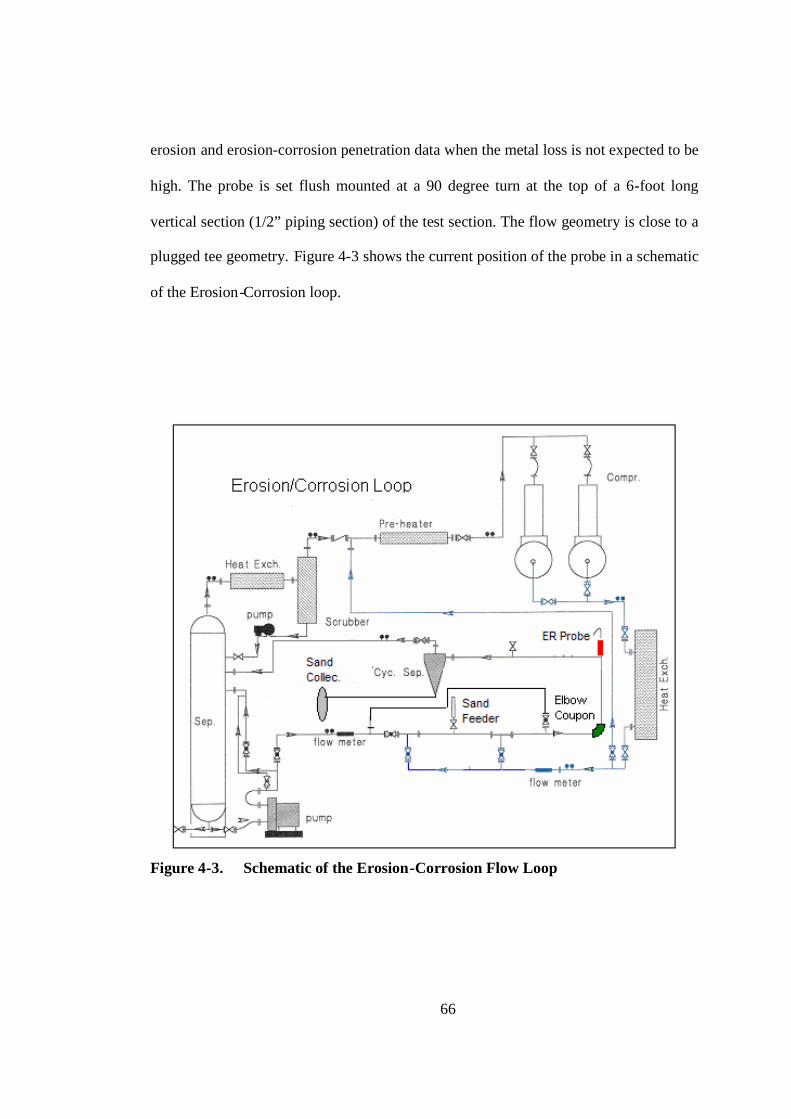
66
erosion and erosion-corrosion penetration data when the metal loss is not expected to be
high. The probe is set flush mounted at a 90 degree turn at the top of a 6-foot long
vertical section (1/2” piping section) of the test section. The flow geometry is close to a
plugged tee geometry. Figure 4-3 shows the current position of the probe in a schematic
of the Erosion-Corrosion loop.
Figure 4-3. Schematic of the Erosion-Corrosion Flow Loop

67
Test cell
Figure 4-4 shows a photograph of the test section of the CO2 loop with the ER
probe set in place (left) and the spiral-shaped-sensor element of the 13Cr ER probe
(right).
Figure 4-4. Photograph of the test section of the Erosion-Corrosion loop with
the ER probe set in place (left). Sensor element of the 13Cr ER
Probe (right).
Test conditions
Electrical resistance measurements in pure erosion and erosion-corrosion in
multiphase flow conditions were performed to see if there is a significant corrosion
component. For pure erosion tests, distilled water and nitrogen were used; for erosion-
corrosion tests 3% brine and CO2 were used. Test conditions are shown in Table 4-1.

68
Table 4-1. Test conditions for erosion and erosion-corrosion tests.
Low Sand Rates High Sand Rates
Material 13Cr 13Cr, Super 13Cr and 22Cr
Flow Geometry 1” Plugged Tee ½” Plugged Tee
Liquid flow velocity 0.2 ft/s 1.4 ft/s
Gas flow velocity 55 and 60 ft/s 20 ft/s
Sand size (avg) 150 microns
Sand rate 1 and 15 lb/day 30 lb/day
Time with sand 5.5 to 6 hours 1 to 3 hours
Solution 3% NaCl* or Distilled water**
Gas Carbon Dioxide* or Nitrogen**
Pressure 50 psig
Temperature 76 and 150 oF
Dissolved Oxygen Less than 10 ppb
pH 4 at 76oF and 4.4 at 150oF
* erosion-corrosion tests ** pure erosion tests
Erosion-Corrosion Liquid/Sand Loop (Microloop)
A smaller experimental facility was designed similar to the Erosion-Corrosion
Multiphase flow loop but for single phase liquid flow. Thus, the loop is capable of
handling CO2-saturated corrosive liquid containing sand. For ease of operation, this

69
facility is much smaller than the former single phase liquid loop (Miniloop) and is
called the Microloop. The main objective of designing the Microloop was to study the
effect of sand concentration and flow velocity on the erosion-corrosion behavior of
corrosion resistance alloys, and thus be able to link the scratch test cell results to
flowing systems containing sand.
Instrumentation and measurement techniques similar to those used in the static
scratch test were used in this facility. Potential and current flowing between the target
working electrode (WE1) and the auxiliary working electrode (WE2) are recorded
during the pre-sand exposure, sand exposure and post-sand exposure period. The
current and potential between the two working electrodes are monitored by a zero
resistance picoammeter and a high resolution and low-noise digital multimeter
respectively. The same software developed to communicate with the instruments for the
Scratch Test was used for Microloop testing.
After some simple mathematical calculations of the measured current data, the
thickness loss and the repassivation time are estimated. As opposed to the scratch test
cell, in the dynamic liquid/sand loop test mechanical and electrochemical processes
involved are taking place simultaneously and continuously, which may make the
analysis of the results quite complex. However, current responses immediately after
removing the sand from the flow provide useful information to determine repassivation
times and the thickness loss that occurred before the material returned to its passive
state.
This Microloop is mainly constructed of 316L SS steel because of its excellent
resistance to corrosion. The major components of this loop are a 10 gallon tank,

70
circulation pump, cyclone separator, test section, sand feeder and sand filter bypass.
Various piping and fittings connect these components to form a closed loop. The safe
working pressure for the Microloop is around 50 psig. Tests were conducted at 20 psig.
A vacuum pump is used to de-aerate and remove dissolved oxygen from the solution. A
band heater around the tank is used to increase the temperature of the solution. This
temperature is maintained in the operating ranges of 100oF to 200oF by using an
electronic controller. The pump is a Wanner Engineering D-3 Hydra-cell diaphragm
pump with a capacity of 3 gpm flow under operating pressures. The pump is the
principal driver and circulates the solution through the loop and back to the tank. The
velocity of the flow through the Microloop is controlled by a variable speed drive for
the pump. This controller allows varying the average flow velocity at the exit of the
direct impingement jet from 10 to 20 ft/s. Lower flow velocities at the jet outlet may be
achieved by bypassing part of the liquid mass directly to the reservoir tank. The
velocity of the flow impinging the test specimen could not be directly measured due to
the small length of the test section which prevented the use of the ultrasonic flow-
meter. However, the velocities were estimated using Bernoulli’s equation. The pressure
differential between the total and static pressure was measured by using a special
straight pitot-tube and a digital manometer.
A schematic of the Microloop is shown in Figure 4-5. The test cell section,
where most of the sand and some liquid are re-circulated, is shown in Figure 4-6. The
sand feeder is de-aerated and pressurized to a pressure slightly higher than the system
pressure (20 psi) to introduce the sand into the system. Sand is introduced into the test
section just upstream of the cyclone separator, where it gets separated from the liquid

71
phase and drops down to the injector nozzle. The sand free liquid flows back to the
tank. The nozzle at the based of the cyclone separator reintroduces the sand into the
flow stream towards the direct impingement test cell. The sand remains recirculating in
the test section until the filter bypass section is engaged and the valve at the top of the
cyclone separator is closed which forces the entire flow to circulate through the 5
micron cartridge filter.
A sand sampling port is provided for measuring the concentration of sand in the
test section as desired. The pH of the solution is monitored using a pH probe housed in
another by-pass section. A pH meter with digital readout is connected to the probe for
accurately measuring the pH during the test. The pH can be controlled by using a
dosing pump which injects acidic or basic solution into the tank as per requirement.
Direct impingement test cell
A direct impingement configuration of the test specimen is used for testing in
the Microloop. Figure 4-7 shows a schematic of the test cell. Two round specimens
made of the same CRA with ½” diameter and ¼” thickness are inserted into a standard
½” cross fitting such that they are perpendicular to each other. The flow coming from
the pump is first accelerated through 1/8” nozzle which discharges into a 5/16” ID
tubing (jet) extended into the cross fitting and terminating very close to the target
specimen (WE1). The flow then, enters the test cell (cross fitting) horizontally through
the jet and directly impinges the target working electrode (WE1), as shown in Figure 4-
7. Flow is diverted vertically upward after impinging the target specimen, leaving the
test cell and moving towards the cyclone separator.
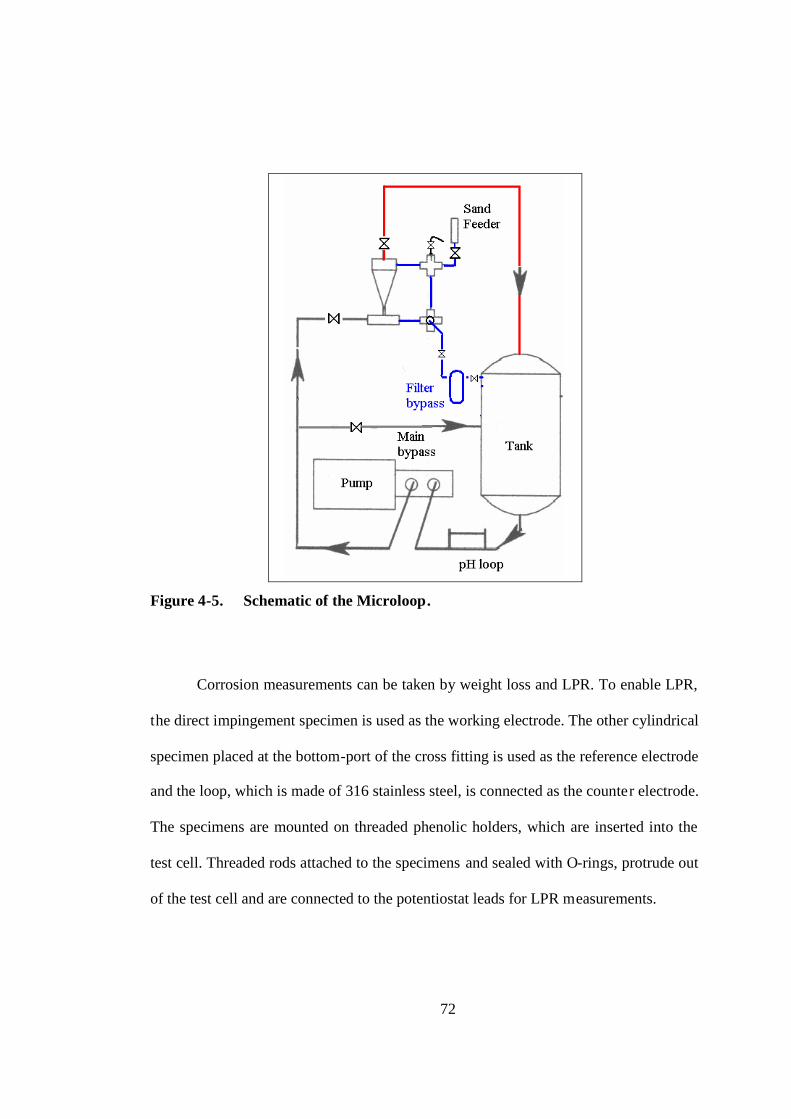
72
Figure 4-5. Schematic of the Microloop.
Corrosion measurements can be taken by weight loss and LPR. To enable LPR,
the direct impingement specimen is used as the working electrode. The other cylindrical
specimen placed at the bottom-port of the cross fitting is used as the reference electrode
and the loop, which is made of 316 stainless steel, is connected as the counter electrode.
The specimens are mounted on threaded phenolic holders, which are inserted into the
test cell. Threaded rods attached to the specimens and sealed with O-rings, protrude out
of the test cell and are connected to the potentiostat leads for LPR measurements.

73
Figure 4-6. Schematic of the test cell section for the Microloop indicating
positions of target working electrode (WE1) and auxiliary working
electrode (WE2).
Figure 4-7. Schematic of the direct impingement test cell for the Microloop
FF
PhenolicHolder
Direct ImpingementSpecimen, WE1
Reference ElectrodeFor LPR, RE
ImpingementJet
Cross Fitting Test

74
A second (or auxiliary) working electrode (WE2, made of the same CRA 2.75”
x 1.425” x 0.275”) is placed upstream of the nozzle and thus is not exposed to the
flowing sand at any time during the test (see test cell section in Figure 4-6). The current
and potential between the two working electrodes are monitored with the same
instrumentation used for the scratch test cell as described above.
Test conditions for liquid/sand loop test
Table 4-2 shows the range of environmental and flow conditions for testing
conducted in the Microloop.
Table 4-2. Test conditions for erosion and erosion-corrosion tests
Erosion-Corrosion Conditions
Material 13Cr and Super 13Cr
Geometry Direct Impingement
Liquid flow velocity 10, 15, 17 and 20 ft/s
Sand size Range (212-272) microns
Sand rate 10 to 860 lb/day
Time with sand 10 min to 240 hours
Solution 3% NaCl
Gas Carbon Dioxide
Pressure 20 psig
Temperature 150 oF
Dissolved Oxygen Less than 10 ppb
pH 4.3 at 150oF

75
Material tested
The material of the working electrodes under investigation are API 5CT L80-
13Cr, referred to as “13Cr” in this report, and a KO-HP2-13Cr-95 referred to as a
“Super 13Cr” (Super 13Cr). The chemical composition of the 13Cr and Super 13Cr are
shown in Table 4-3 Table 4-4, respectively. For comparison purposes, the UNS 2205
alloy referred to as “22Cr” in this report was also tested at some of the most aggressive
conditions and its chemical composition is shown in Table 4-5
Table 4-3. The chemical composition of 13Cr.
C Si Mn P S Cr Ni Mo Cu Fe
min 0.15 - 0.25 - - 12.0 - - - -
max 0.22 1.00 1.00 0.020 0.010 14.0 0.50 - 0.25 -
Ladle 0.18 0.28 0.45 0.020 0.002 12.91 0.11 0.00 0.01 Bal
Table 4-4. The chemical composition of Super 13Cr.
C Si Mn P S Cr Ni Mo Cu Fe
min - - 0.30 - - 12.00 3.50 1.50 - -
max 0.040 0.50 0.60 0.020 0.005 14.00 5.50 2.50 0.25 -
Ladle 0.020 0.19 0.44 0.018 0.001 12.85 5.35 2.14 0.10 Bal
Table 4-5. The chemical composition of the 22Cr.
C Si Mn P S Cr Ni Mo Cu Fe
min - - - - - 21.0 4.5 2.5 - -
max 0.030 1.00 2.00 0.030 0.020 23.0 6.5 3.5 - -
Ladle 0.018 0.40 0.480 0.026 0.015 22.62 5.51 3.38 0.20 Bal
76
CHAPTER 3 ..............................................................................................................................57
OBJECTIVES AND APPROACH................................................................................................ ....57
Research Objectives................................................................................................ ...........57
Approach................................ ............................................................................................58
CHAPTER 4 ..............................................................................................................................61
EXPERIMENTAL PROCEDURE AND TESTING CONDITIONS ..........................................................61
Scratch Test Experimental Setup .......................................................................................61
Test Matrix ......................................................................................................................................... 64
Erosion-Corrosion-Loop (Gas/Liquid/Sand Multiphase Flow Loop) ...............................64
Test cell ............................................................................................................................................... 67
Test conditions ................................................................................................................................... 67
Erosion-Corrosion Liquid/Sand Loop (Microloop) ...........................................................68
Direct impingement test cell.............................................................................................................. 71
Test conditions for Liquid/Sand Loop Test ...................................................................................... 74
Material tested .................................................................................................................................... 75
TABLE 4-1. TEST CONDITIONS FOR EROSION AND EROSION-CORROSION TESTS......................................68
TABLE 4-2. TEST CONDITIONS FOR EROSION AND EROSION-CORROSION TESTS .....................................74
TABLE 4-3. THE CHEMICAL COMPOSITION OF 13CR. ................................................................ .............75
TABLE 4-4. THE CHEMICAL COMPOSITION OF SUPER 13CR. ..................................................................75
TABLE 4-5. THE CHEMICAL COMPOSITION OF THE 22CR. ................................................................ ......75
FIGURE 4-1. LAYOUT OF THE ELECTROCHEMICAL CELL FOR SCRATCH TEST. ................................ ....62
FIGURE 4-2. SET-UP FOR ELECTROCHEMICAL MEASUREMENTS FOR SCRATCH TEST...............................63
FIGURE 4-3. SCHEMATIC OF THE EROSION-CORROSION FLOW LOOP................................ ......................66
FIGURE 4-4. PHOTOGRAPH OF THE TEST SECTION OF THE EROSION-CORROSION LOOP WITH THE ER
PROBE SET IN PLACE (LEFT). SENSOR ELEMENT OF THE 13CR ER PROBE (RIGHT). ............................67
FIGURE 4-5. SCHEMATIC OF THE MICROLOOP....................................................................................72
FIGURE 4-6. SCHEMATIC OF THE TEST CELL SECTION FOR THE MICROLOOP INDICATING POSITIONS OF
TARGET WORKING ELECTRODE (WE1) AND AUXILIARY WORKING ELECTRODE (WE2). .....................73
FIGURE 4-7. SCHEMATIC OF THE DIRECT IMPINGEMENT TESTCELL FOR THE MICROLOOP .................73

77

76
CHAPTER 5
SCRATCH TEST AS A SIMPLIFIED EROSION-CORROSION TEST
Motivation for Doing Scratch Test
A laboratory method previously introduced by McMahon and Martin60 was used
to study the effect of pH and temperature on the repassivation behavior of CRAs in CO2-
saturated brines. The laboratory method was conducted in a glass cell. Data were
collected based on an electrochemical technique. The working electrode (CRA) is
scratched while the potential and current are recorded. After some simple mathematical
calculations, the thickness loss and the repassivation time can be estimated. The scratch
made on a well-defined area of the working electrode may be interpreted as similar to the
removal of the passive layer due to a single particle impingement, and it is believed that
this approach can be used to study the effect of erosion on the corrosion response. With
scratch tests, the mechanical process of making the scratch and the repassivation process
of a CRA can be viewed as nearly separate events. The sand erosion process bears some
similarity to a simple scratch test except that mechanical and electrochemical processes
involved are taking place simultaneously and continuously. The goal of investigating the
simple scratch test was to shed some light on the erosion-corrosion behavior of CRAs.

77
The effects of pH and temperature on the repassivation of 13Cr, Super 13Cr and
22Cr were thoroughly examined, and a summary of the results are presented later in this
chapter. First, the data reduction techniques for the measurements obtained from the
scratch test are described in the following section.
Data Reduction Technique
For a typical scratch test, the initial anodic current is very high immediately after
making the scratch. Figure 5-1 shows a typical current decay with time during a scratch
healing process for a 13Cr alloy exposed to 3.5% brine solution at pH 4 and temperature
of 76oF. The three CRAs show similar behavior for all conditions tested. How fast the
current decays with time is determined by the healing rate of the oxide film which
depends on many variables such as temperature, pH, flow velocity, and material tested.
0
5
10
15
20
25
30
35
40
45
50
55
0 20 40 60 80 100 120 140 160 180 200
Time (sec)
Cu
rren
t,I
( mA
)
76 oF, pH = 4, 13Cr
Figure 5-1. Anodic current decay during the scratch repassivation process.

78
The anodic current decay for CRAs was characterized as approximately following
the second order behavior at least for the first 200 seconds of the scratch repassivation
process expressed by the equation (5-1).
mIdtdI 2 (5-1)
where, I is the measured current, t is time, and m is a constant that depends on material
and environmental conditions. The “second order” is used here to denote that the rate of
change of current, I, with respect to time is proportional to I2. Integration of equation (5-
1) yields:
mtII
I0
0
1 or mt
II
0
11 (5-2)
where, Io is the initial current at t = 0.
Equation (5-2) suggests Io and m can be conveniently obtained from a plot of 1/I
vs. time as shown in Figure 5-2, which contains the same data shown in Figure 5-1.
1/I = 1,774 t + 36,067
0.0E+00
1.0E+05
2.0E+05
3.0E+05
4.0E+05
5.0E+05
0 50 100 150 200
Time (sec)
1/I
(1/A
)
76 oF, pH = 4, 13Cr
Figure 5-2. Data showing a linear relation between 1/I and time.

79
Equation (5-2) can be integrated and presented in a convenient form to
characterize the healing process as a protective film growth process. Estimation of the
cumulative thickness loss (TL) at any time t = t* is given by:
)1ln( 0
*
0
tmImCdtICTL
t
(5-3)
where, C accounts for units conversion factor and some material properties, t* is the
repassivation time defined as the time required for the current to return to a specific value
of I* (e.g., I* is the current at the passive state corresponding to a corrosion rate of about
1 mpy), then from equation (5-2), the repassivation time, is given by:
0
11ImIm
t
(5-4)
This means that knowing m and Io, the time required for the corrosion rate to
return to one mpy, or other appropriate limit, can be predicted.
An expression for the TL accumulated by the time the CRAs repassivate can be
derived by substituting equation (5-4) into equation (5-3), yielding:
II
mC
ImImIm
mCTL 0
00 ln111ln (5-5)
Figure 5-3 shows the comparison of the actual cumulative thickness loss (TLactual)
and the calculated cumulative thickness loss (TLcal) for 13Cr from the raw data displayed
in Figure 5-1. Good agreement is obtained.
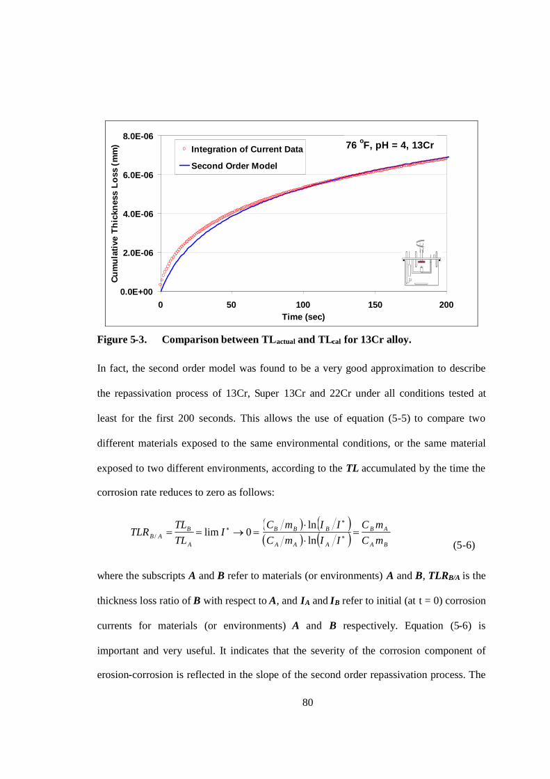
80
0.0E+00
2.0E-06
4.0E-06
6.0E-06
8.0E-06
0 50 100 150 200Time (sec)
Cu
mu
lati
veT
hic
knes
sL
oss
(mm
) Integration of Current Data
Second Order Model
76 oF, pH = 4, 13Cr
Figure 5-3. Comparison between TLactual and TLcal for 13Cr alloy.
In fact, the second order model was found to be a very good approximation to describe
the repassivation process of 13Cr, Super 13Cr and 22Cr under all conditions tested at
least for the first 200 seconds. This allows the use of equation (5-5) to compare two
different materials exposed to the same environmental conditions, or the same material
exposed to two different environments, according to the TL accumulated by the time the
corrosion rate reduces to zero as follows:
BA
AB
AAA
BBB
A
BAB mC
mCIImCIImC
ITLTL
TLR
lnln
0lim/
(5-6)
where the subscripts A and B refer to materials (or environments) A and B, TLRB/A is the
thickness loss ratio of B with respect to A, and IA and IB refer to initial (at t = 0) corrosion
currents for materials (or environments) A and B respectively. Equation (5-6) is
important and very useful. It indicates that the severity of the corrosion component of
erosion-corrosion is reflected in the slope of the second order repassivation process. The
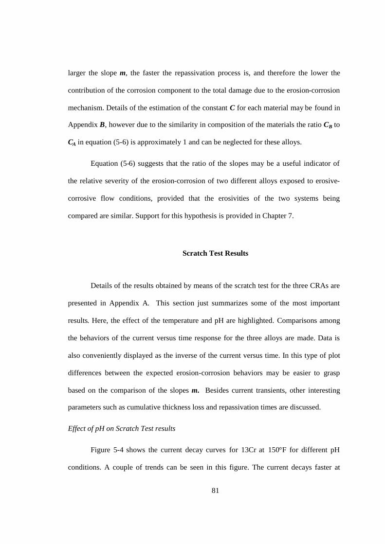
81
larger the slope m, the faster the repassivation process is, and therefore the lower the
contribution of the corrosion component to the total damage due to the erosion-corrosion
mechanism. Details of the estimation of the constant C for each material may be found in
Appendix B, however due to the similarity in composition of the materials the ratio CB to
CA in equation (5-6) is approximately 1 and can be neglected for these alloys.
Equation (5-6) suggests that the ratio of the slopes may be a useful indicator of
the relative severity of the erosion-corrosion of two different alloys exposed to erosive-
corrosive flow conditions, provided that the erosivities of the two systems being
compared are similar. Support for this hypothesis is provided in Chapter 7.
Scratch Test Results
Details of the results obtained by means of the scratch test for the three CRAs are
presented in Appendix A. This section just summarizes some of the most important
results. Here, the effect of the temperature and pH are highlighted. Comparisons among
the behaviors of the current versus time response for the three alloys are made. Data is
also conveniently displayed as the inverse of the current versus time. In this type of plot
differences between the expected erosion-corrosion behaviors may be easier to grasp
based on the comparison of the slopes m. Besides current transients, other interesting
parameters such as cumulative thickness loss and repassivation times are discussed.
Effect of pH on Scratch Test results
Figure 5-4 shows the current decay curves for 13Cr at 150°F for different pH
conditions. A couple of trends can be seen in this figure. The current decays faster at

82
higher pH as indicated by the greater initial slopes shown for pH 5.25 and 6 as compared
to lower pH values (3.5 or 4). Also, the value of the current observed is lower at higher
pH (5.25 or 6) than for lower pH (3.5 or 4) over the entire interval of 200 seconds shown
in the figure. Since the corrosion rates are proportional to the current, these results
suggest very high corrosion rates immediately after making the scratch and exposing the
bare metal to the corrosive solution. Then corrosion rates decay with time while the
healing process takes place on the metallic surface. The passivated state is achieved faster
for higher pH’s. For the other temperatures, namely 76°F and 200°F, similar trends with
pH are observed (results are included in Appendix A). However the initial currents
obtained immediately after making the scratch for these temperatures are lower at 76oF
and higher at 200oF than the current obtained for 150oF.
Figure 5-5 shows the current decay curves for Super 13Cr at different pH
conditions at 150°F. Trends observed in this figure for Super 13Cr seem to be similar to
those observed for 13Cr in Figure 5-4, i.e., the current decays at faster rates at higher pH
than it does it for low pH. Also the value of the initial current is lower for higher pH.
However, variations in the Super 13Cr current response due to changes in pH are less
evident than those showed by 13Cr. Current transients trends with pH for Super 13Cr
obtained at 76°F and 200°F are similar to that observe for 150oF (see Appendix A). They
all seem to have same trends with pH as those shown for 13Cr in Figure 5-4; but, current
transients for Super 13Cr for all pH are very close to each other and overlap in a very
narrow range which makes it difficult to observe the trend of the response of the Super
13Cr with pH. However plots of 1/I vs. time for the same data included in Appendix A
showed the trends more clearly.

83
0
20
40
60
80
100
120
140
0 50 100 150 200Time (sec)
I( m
A)
pH = 3.5
pH = 4.0pH = 5.25
pH = 6.0
13Cr AlloyT = 150ºF
Figure 5-4. Effect of pH on the decay of the anodic current after a scratch has
been made on the surface of a 13Cr Alloy.
0
20
40
60
80
100
120
140
0 50 100 150 200Time (sec)
I(mA
)
pH = 3.5pH = 4.0
pH = 5.25, and pH = 6.0
Super13Cr AlloyT = 150ºF
Figure 5-5. Effect of pH on the decay of the anodic current after a scratch has
been made on the surface of a Super 13Cr Alloy.
Figure 5-6 shows 1/I versus time t for the same raw data used in Figure 5-4. Good
linearity between 1/I and time t in all pH conditions at room 150°F indicates that the

84
repassivation processes in these conditions all follow approximately second order
behavior at least for the first 200 seconds. According to equation (5-6), the thickness loss
ratio between two different conditions for the same material is the reciprocal of the ratio
of corresponding slopes in the 1/I versus time t charts. As shown in Figure 5-6, the slope
at pH = 3.5, is lower (mpH=3.5= 485) than the slope at pH =4.0 (mpH=4= 1063) which is
much lower than the slope for pH = 6 (mpH=6.0= 2159). Therefore, the corrosion
component of the erosion-corrosion damage at pH 3.5 should be about 2.2 times more
severe than at pH 4.0, and about 4.5 times more severe than at pH 6.0. These results
indicate how significant the effect of pH is on the repassivation process of 13Cr at tested
conditions. Similar plots for 76 and 200oF are found in Appendix A.
0.E+00
2.E+05
4.E+05
6.E+05
0 50 100 150 200Time (sec)
1/I,
(1/A
)
pH=4.0
pH=5.25
pH=3.5
pH=6.0T= 150ºF13Cr
Figure 5-6. 1/I vs. t for 13Cr from the raw scratch test data in Figure 5-4.
Figure 5-7 is the 1/I versus time t chart for Super 13Cr at 150°F from the raw data
in Figure 5-5. The trend of the slope with pH observed for this alloy is similar to that
observed for 13Cr, mpH=6.0 > mpH=5.25> mpH=3.5, which predicts a lower corrosion

85
component of the erosion-corrosion process for higher pH values. Notice that slopes for
Super 13Cr at different pH values are clustered closer together as compared with those
for 13Cr; hence, the effect of pH on the erosion-corrosion damage of Super13Cr is
expected to be smaller than that experienced by 13Cr. Again trends for 76 and 150oF are
found in Appendix A.
0.E+00
2.E+05
4.E+05
6.E+05
0 50 100 150 200Time (sec)
1/I,
(1/A
)
pH=4.0, & 3.5
pH=5.25pH=6.0
T= 150ºFSuper 13Cr
Figure 5-7. 1/I vs. t for 13Cr from the raw data in Figure 5-5.
Effect of temperature on Scratch Test results
Figure 5-8 shows the comparison of the current decays for 13Cr scratch tests
conducted at different temperatures, 76, 150 and 200oF but for a fixed pH of 4. As
expected, at higher temperatures, higher healing rates were found as suggested by the
steeper slopes shown by the current vs. time curves at 200oF. However, the higher
temperature always causes a current that is initially higher and remains higher over the
entire test period than for a lower temperature. As a result, at higher temperatures, it takes

86
a longer time for the current to return to its original level. Therefore, the cumulative
thickness loss after making the scratch is expected to be higher for higher temperatures,
as shown in Figure 5-9. Similar trends are obtained for other pH values (3.5, 5.25 and
6.0), and results are included in Appendix A.
0
20
40
60
80
100
120
140
160
180
200
0 50 100 150 200Time (sec)
I(mA
)
13Cr AlloypH= 4.0
200oF
150oF
76oF
Figure 5-8. Effect of temperature on the decay of the anodic current after a
scratch has been performed on the surface of a 13Cr Alloy.
Figure 5-10 and Figure 5-11 show the effect of temperature on the current decays
for Super 13Cr and 22Cr, respectively. The trend of the current decay with temperature
for Super 13Cr and 22Cr is similar to the one observed for 13Cr. The higher the
temperature, the higher the currents were for the three alloys. However, results suggest
that the effect of temperature on the current transients is significantly stronger for 13Cr
than it is for Super 13Cr and 22Cr. In fact, for 22Cr no clear distinction among the
behaviors of the current transients with temperature after the first 20 seconds was found.

87
13Cr AlloypH=4.0
0.0E+00
4.0E-06
8.0E-06
1.2E-05
1.6E-05
2.0E-05
2.4E-05
2.8E-05
3.2E-05
0 50 100 150 200Time (sec)
Thic
knes
sLo
ss(m
m)
13Cr, T=76oF
13Cr, T=150oF
13Cr, T=200oF
Figure 5-9. Effect of temperature on the cumulative thickness loss experienced by
13Cr after being scratched at pH=4.0.
0
20
40
60
80
100
120
140
160
180
200
0 50 100 150 200Time (sec)
I( m
A)
Super 13Cr AlloypH= 4.0
200oF
150oF76
oF
Figure 5-10. Effect of temperature on the decay of the anodic current after a
scratch has been performed on the surface of a Super 13Cr Alloy.

88
0
5
10
15
20
25
30
35
40
45
50
0 50 100 150 200Time (sec)
I (mA
)
200oF
150oF76oF
22Cr AlloypH= 4.0
Figure 5-11. Effect of temperature on the decay of the anodic current after a
scratch has been performed on the surface of a 22Cr Alloy.
At the elevated temperatures, the 1/I slopes (for a fixed pH) are smaller than
slopes found at lower temperatures, which indicates the longer repassivation times
needed to reform the passive film at higher temperatures. Trends of the 1/I slopes with
temperature at pH 4 for the three alloys are clearly seen in Figure 5-12 to Figure 5-14. At
a given pH, mT=76 > mT=150> mT=200 which predicts higher corrosion components of the
erosion-corrosion process for higher temperatures. Notice that slopes for 22Cr at different
temperatures are closer together than those for Super 13Cr and 13Cr; hence, the effect of
temperature on the erosion-corrosion damage of 22Cr is expected to be smaller than that
experienced by Super13Cr and 13Cr. The effect of temperature at other pH values
showed trends similar to those shown for pH = 4 (Appendix A)

89
0.E+00
1.E+05
2.E+05
3.E+05
4.E+05
0 50 100 150 200Time (sec)
1/I,
(1/A
)
13CrpH= 4.0
T=200oF
T=150oF
T=76oF
Figure 5-12. 1/I vs. t for 13Cr from the raw data in Figure 5-8.
0.E+00
1.E+05
2.E+05
3.E+05
4.E+05
0 50 100 150 200Time (sec)
1/I
,(1
/A)
Super 13CrpH= 4.0
T=76oFT=150oF
T=200oF
Figure 5-13. 1/I vs. t for 13Cr from the raw data in Figure 5-10.
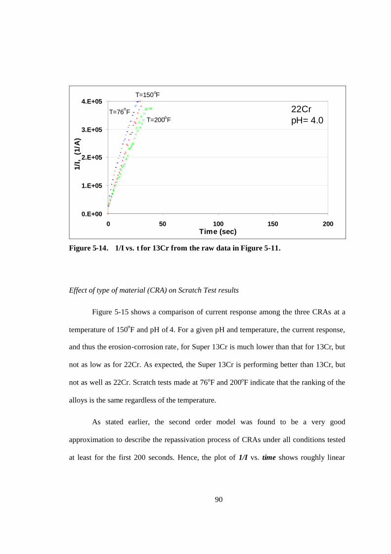
90
0.E+00
1.E+05
2.E+05
3.E+05
4.E+05
0 50 100 150 200Time (sec)
1/I,
(1/A
)
22CrpH= 4.0T=200oF
T=76oF
T=150oF
Figure 5-14. 1/I vs. t for 13Cr from the raw data in Figure 5-11.
Effect of type of material (CRA) on Scratch Test results
Figure 5-15 shows a comparison of current response among the three CRAs at a
temperature of 150oF and pH of 4. For a given pH and temperature, the current response,
and thus the erosion-corrosion rate, for Super 13Cr is much lower than that for 13Cr, but
not as low as for 22Cr. As expected, the Super 13Cr is performing better than 13Cr, but
not as well as 22Cr. Scratch tests made at 76oF and 200oF indicate that the ranking of the
alloys is the same regardless of the temperature.
As stated earlier, the second order model was found to be a very good
approximation to describe the repassivation process of CRAs under all conditions tested
at least for the first 200 seconds. Hence, the plot of 1/I vs. time shows roughly linear
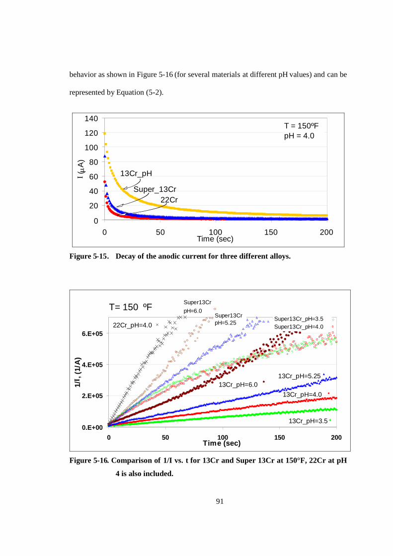
91
behavior as shown in Figure 5-16 (for several materials at different pH values) and can be
represented by Equation (5-2).
0
20
40
60
80
100
120
140
0 50 100 150 200Time (sec)
I (mA
)
13Cr_pH
22CrSuper_13Cr
T = 150ºFpH = 4.0
Figure 5-15. Decay of the anodic current for three different alloys.
0.E+00
2.E+05
4.E+05
6.E+05
0 50 100 150 200Time (sec)
1/I ,
(1/A
)
13Cr_pH=4.0
13Cr_pH=5.25
13Cr_pH=3.5
13Cr_pH=6.0
T= 150 ºF
22Cr_pH=4.0Super13Cr_pH=3.5Super13Cr_pH=4.0
Super13CrpH=6.0
Super13CrpH=5.25
Figure 5-16. Comparison of 1/I vs. t for 13Cr and Super 13Cr at 150°F, 22Cr at pH
4 is also included.

92
For a given pH and temperature, the Super 13Cr slope is larger than the
corresponding slope found for 13Cr, which indicates a shorter repassivation time is
needed for Super 13Cr to reform the passive film at similar conditions. At a pH of 4,
m22Cr > mSuper 13Cr> m13Cr at 76, 150 or 200oF, which indicates the highest corrosion rate
of the erosion-corrosion process is for 13Cr and the lowest is for 22Cr, while the Super
13Cr corrosion rate lies between.
Cumulative Thickness Loss and Repassivation Time
Appendix A contains the cumulative thickness loss data based on the integration
of all the current data presented in the previous three sections. From these charts, the
trends are very clear. For a fixed temperature, the corrosion component of the erosion-
corrosion damage is more severe at lower pH values where cumulative thickness losses
are higher. Also notice that the thickness loss for a fixed pH is higher for higher
temperatures. In general, for a given pH and temperature, the cumulative thickness losses
for Super 13Cr are much lower than those for 13Cr, but not as low as for 22Cr. This
relation would predict less erosion-corrosion damage on 22Cr than on Super 13Cr or
13Cr.
As a convenient form of summarizing all the scratch test data in a single plot the
cumulative thickness loss after 200 seconds is shown in Figure 5-17 for the three CRAs
using two different approaches. The first approach is the estimation of the cumulative
thickness loss obtained from integration of the current data time series up to 200 seconds.

93
The second approach, the estimation of the cumulative thickness loss at time t = 200 s
was made by means of the second order approximation using equation (5-3).
As can be seen from Figure 5-17 the higher the temperature the higher the metal
thickness loss due to the corrosion component of the erosion-corrosion process. The three
alloys showed the same trend with temperature. Regardless of temperature the 13Cr
presented the highest thickness loss and the 22Cr the lowest. Figure 5-18 shows the effect
of temperature on the ratios of the thickness loss of 13Cr to Super 13Cr and 22Cr at pH =
4 (from data shown in Figure 5-17). Notice the thickness loss for 13Cr at 76 oF is about
twice the thickness loss of the Super 13Cr and about 5 times the thickness loss of the
22Cr at the same temperature. These factors increase slightly with increasing temperature
as shown in Figure 5-18.
0.0E+00
5.0E-06
1.0E-05
1.5E-05
2.0E-05
2.5E-05
3.0E-05
Thic
knes
sL
oss
(mm
)
13Cr, I dataIntegration
13Cr2ndOrder
S13Cr, I dataIntegration
S13Cr2ndOrder
22Cr, I dataIntegration
22Cr2ndOrder
76
150200
Corrosion Resistant Alloy
Temp.
(oF)
76150200
200
15076
pH = 4
Figure 5-17. Comparison of the cumulative thickness loss after 200 seconds for the
three CRAs at pH = 4 and different temperatures.
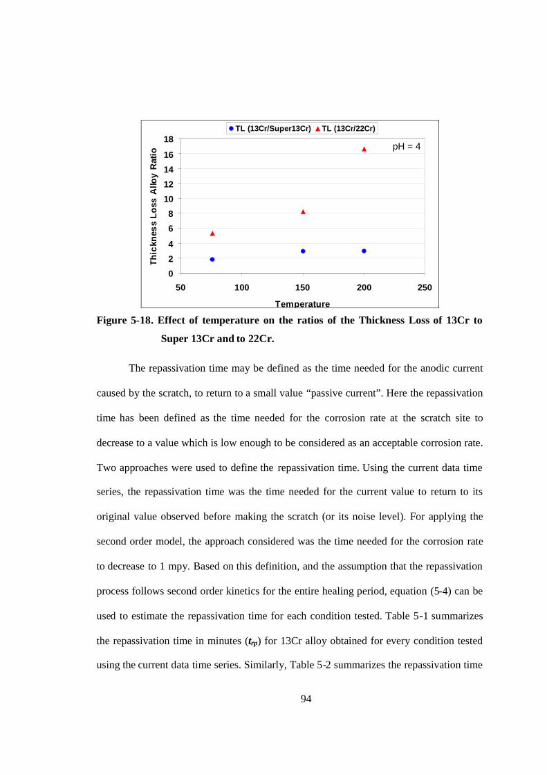
94
0
2
4
6
8
10
12
14
16
18
50 100 150 200 250
Temperature
Th
ickn
ess
Lo
ssA
lloy
Rat
io
TL (13Cr/Super13Cr) TL (13Cr/22Cr)
pH = 4
Figure 5-18. Effect of temperature on the ratios of the Thickness Loss of 13Cr to
Super 13Cr and to 22Cr.
The repassivation time may be defined as the time needed for the anodic current
caused by the scratch, to return to a small value “passive current”. Here the repassivation
time has been defined as the time needed for the corrosion rate at the scratch site to
decrease to a value which is low enough to be considered as an acceptable corrosion rate.
Two approaches were used to define the repassivation time. Using the current data time
series, the repassivation time was the time needed for the current value to return to its
original value observed before making the scratch (or its noise level). For applying the
second order model, the approach considered was the time needed for the corrosion rate
to decrease to 1 mpy. Based on this definition, and the assumption that the repassivation
process follows second order kinetics for the entire healing period, equation (5-4) can be
used to estimate the repassivation time for each condition tested. Table 5-1 summarizes
the repassivation time in minutes (trp) for 13Cr alloy obtained for every condition tested
using the current data time series. Similarly, Table 5-2 summarizes the repassivation time

95
in minutes (trp) for 13Cr at every condition tested estimated using the second order
kinetics approximation. Trends are similar for the two approaches. The repassivation
times are longer for higher temperatures and shorter for higher pH. These results suggest
that the corrosion component of the erosion-corrosion phenomenon on 13Cr is more
severe for higher temperatures and lower pH.
Repassivation times in minutes, for Super 13 Cr and 22Cr, for both approaches
are shown in Table 5-3. In general, the repassivation times for Super 13Cr and 22Cr were
much lower than those for 13Cr at similar conditions; 22Cr having the lowest
repassivation times. The trend of repassivation time with temperature for Super 13Cr is
similar to that seen for 13Cr: the higher the temperature, the longer the time needed to
obtain the original low current values. The effects of pH on repassivation times are also
similar for both 13Cr and Super 13Cr; but, Super 13Cr data are just shown for pH 4. No
clear trend was observed for the effect of temperature on the repassivation times of 22Cr
since the data points for different temperatures are so close to each other for 22Cr.
Table 5-1. Repassivation times in minutes for 13Cr at different test conditions using
current data time series approach.
T
pH
76°F 150°F 200°F
3.50 112 148 169
4.00 34 136 262
4.75 19 102 185
5.25 16 66 78
6.00 3 34 30

96
Table 5-2. Repassivation times in minutes for 13Cr at different test conditions using
2nd order kinetics approximation.
T
pH
76°F 150°F 200°F
3.50 155 187 339
4.00 43 104 209
4.75 33 90 187
5.25 22 71 55
6.00 5 43 84
Table 5-3. Repassivation times in minutes at pH = 4 and the three temperatures for
Super 13Cr and 22Cr using both approaches, current data time seriesapproach and 2nd order kinetics approximation.
Material 76°F 150°F 200°F
From current data time
series. Super13Cr 17 25 51
From 2nd Order kinetics
approx. Super 13Cr 18 26 74
From current data timeseries. 22Cr 8 12 5
From 2nd Order kinetic
approx. 22Cr 8 11 9
Trends for repassivation times of 13Cr and Super 13Cr using both approaches are
also clearly seen on Figure 5-19 and Figure 5-20 where data for 22Cr at pH = 4 and the
three temperatures are also included for comparison purposes. Trend lines as straight
lines are included to aid the viewing of trends; however, pH repassivation time and
temperature repassivation time relations may not be linear. As can be seen, the

97
repassivation times for Super 13Cr and 22Cr are much shorter than those for 13Cr for a
fixed pH and temperature, which indicates that Super 13Cr and 22Cr heal much faster
than 13Cr at the same conditions, with 22Cr being the fastest. Comparisons of
repassivation times among the three alloys are more clearly seen for pH 4 in Figure 5-21.
Figure 5-22 shows the comparison between repassivation times provided by the
current data time series and the repassivation times estimated from the second order
kinetics approximation. As can be seen, the agreement is very good, particularly for
repassivation times of 50 minutes and below. The most scattered data points (diamonds)
belong to 200oF testing and may be explained as due to experimental limitations in
keeping the test solution from evaporating in a bubbling test cell setup (for 13Cr testing).
A new closed experimental setup was designed to keep the pressure slightly above
atmospheric pressure reducing liquid evaporation and reducing data scatter (Super 13Cr
data).

98
0
40
80
120
160
200
240
280
3.0 3.5 4.0 4.5 5.0 5.5 6.0 6.5pH
Rep
assi
vati
on
tim
e(m
in) 200
150
76
200 (S13Cr)
150 (S13Cr)
76 (S13Cr)
200 (22Cr)
150 (22Cr)
76 (22Cr)
T (oF)
13Cr 200 oF13Cr 150 oF
13Cr 76 oFS13Cr 200 oF
} 22Cr All Temp.
S13Cr 150 oFS13Cr 76 oF
Figure 5-19. Effect of pH and temperature on the repassivation times of 13Cr at
different test conditions. Data for Super 13Cr and 22Cr at pH 4 and
the three temperatures are also included.
0
10
20
30
40
50
60
3.0 3.5 4.0 4.5 5.0 5.5 6.0 6.5
pH
Rep
assi
vatio
ntim
e(m
in) 200 (S13Cr)
150 (S13Cr)
76 (S13Cr)
200 (22Cr)
150 (22Cr)
76 (22Cr)
T (oF)S13Cr 200 oF
S13Cr 150 oF
S13Cr 76 oF
22Cr 200 oF
22Cr 150 oF
22Cr 76 oF
Figure 5-20. Effect of pH and temperature on the repassivation times of Super
13Cr at different test conditions. Data for 22Cr at pH 4 and the three
temperatures are also included.
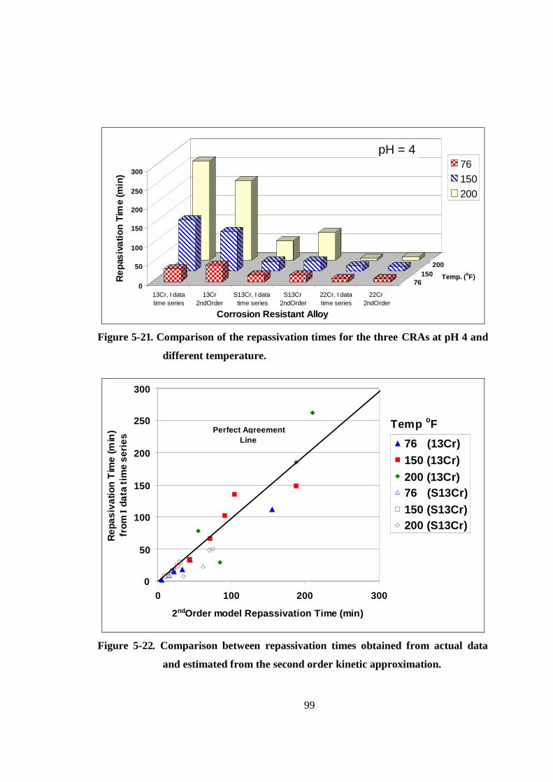
99
0
50
100
150
200
250
300
Rep
asiv
atio
nTi
me
(min
)
13Cr, I datatime series
13Cr2ndOrder
S13Cr, I datatime series
S13Cr2ndOrder
22Cr, I datatime series
22Cr2ndOrder
76
150
200
Corrosion Resistant Alloy
Temp. (oF)
76150200
200150
76
pH = 4
Figure 5-21. Comparison of the repassivation times for the three CRAs at pH 4 and
different temperature.
0
50
100
150
200
250
300
0 100 200 300
2ndOrder model Repassivation Time (min)
Rep
asiv
atio
nT
ime
(min
)fr
omI
data
tim
ese
ries 76 (13Cr)
150 (13Cr)200 (13Cr)76 (S13Cr)150 (S13Cr)200 (S13Cr)
Temp oFPerfect AgreementLine
Figure 5-22. Comparison between repassivation times obtained from actual data
and estimated from the second order kinetic approximation.

100
CHAPTER 5 ..................................................................................................................................76
SCRATCH TEST AS A SIMPLIFIED EROSION-CORROSION TEST .....................................................76
Motivation for Doing Scratch Test ................................................................ ........................76
Data reduction technique ................................ ................................................................ ......77
Scratch Test Results................................ ................................................................ ...............81
Effect of pH on Scratch Test results ..................................................................................................... 81
Effect of temperature on Scratch Test results....................................................................................... 85
Effect of type of material (CRA) on Scratch Test results.................................................................... 90
Cumulative Thickness Loss and Repassivation Time ............................................................92
FIGURE 5-1. ANODIC CURRENT DECAY DURING THE SCRATCH REPASSIVATION PROCESS. ..........................77
FIGURE 5-2. DATA SHOWING A LINEAR RELATION BETWEEN 1/I AND TIME. ................................ ...............78
FIGURE 5-3. COMPARISON BETWEEN TLACTUAL AND TLCAL FOR 13CR ALLOY. ................................ ......80
FIGURE 5-4. EFFECT OF PH ON THE DECAY OF THE ANODIC CURRENT AFTER A SCRATCH HAS BEEN MADE
ON THE SURFACE OF A 13CR ALLOY................................................................................................. ....83
FIGURE 5-5. EFFECT OF PH ON THE DECAY OF THE ANODIC CURRENT AFTE R A SCRATCH HAS BEEN MADE
ON THE SURFACE OF A SUPER 13CR ALLOY..........................................................................................83
FIGURE 5-6. 1/I VS. T FOR 13CR FROM THE RAW SCRATCH TEST DATA IN FIGURE 5-4. ...............................84
FIGURE 5-7. 1/I VS. T FOR 13CR FROM THE RAW DATA IN FIGURE 5-5. .......................................................85
FIGURE 5-8. EFFECT OF TEMPERATURE ON THE DECAY OF THE ANODIC CURRENT AFTER A SCRATCH HAS
BEEN PERFORMED ON THE SURFACE OF A 13CR ALLOY........................................................................86
FIGURE 5-9. EFFECT OF TEMPERATURE ON THE CUMULATIVE THICKNESS LOSS EXPERIENCED BY 13CR
AFTER BEING SCRATCHED AT PH=4.0. ..................................................................................................87
FIGURE 5-10. EFFECT OF TEMPERATURE ON THE DECAY OF THE ANODIC CURRENT AFTER A SCRATCH HAS
BEEN PERFORMED ON THE SURFACE OF A SUPER 13CR ALLOY.............................................................87
FIGURE 5-11. EFFECT OF TEMPERATURE ON THE DECAY OF THE ANODIC CURRENT AFTER A SCRATCH HAS
BEEN PERFORMED ON THE SURFACE OF A 22CR ALLOY........................................................................88
FIGURE 5-12. 1/I VS. T FOR 13CR FROM THE RAW DATA IN FIGURE 5-8. ..................................................89
FIGURE 5-13. 1/I VS. T FOR 13CR FROM THE RAW DATA IN FIGURE 5-10. ................................................89
FIGURE 5-14. 1/I VS. T FOR 13CR FROM THE RAW DATA IN FIGURE 5-11. ................................................90
FIGURE 5-15. DECAY OF THE ANODIC CURRENT FOR THREE DIFFERENT ALLOYS................................. ....91
FIGURE 5-16. COMPARISON OF 1/I VS. T FOR 13CR AND SUPER13CR AT 150°F, 22CR AT PH4 IS ALSO
INCLUDED................................. ............................................................................................................91
FIGURE 5-17. COMPARISON OF THE CUMULATIVE THICKNESS LOSS AFTER 200 SECONDS FOR THE THREE
CRAS AT PH = 4 AND DIFFERENT TEMPERATURES................................................................. ...............93

101
FIGURE 5-18. EFFECT OF TEMPERATURE ON THE RATIOS OF THE THICKNESS LOSS OF 13CR TO SUPER 13CR
AND TO 22CR........................................................................................................................................94
FIGURE 5-19. EFFECT OF PH AND TEMPERATURE ON THE REPASSIVATION TIMES OF 13CR AT DIFFERENT TEST
CONDITIONS. DATA FOR SUPER 13CR AND 22CR AT PH 4 AND THE THREE TEMPERATURES ARE ALSO
INCLUDED................................. ............................................................................................................98
FIGURE 5-20. EFFECT OF PH AND TEMPERATURE ON THE REPASSIVATION TIMES OF SUPER 13CR AT
DIFFERENT TEST CONDITIONS. DATA FOR22CR AT PH 4 AND THE THREE TEMPERATURES ARE ALSO
INCLUDED. 98
FIGURE 5-21. COMPARISON OF THE REPASSIVATION TIMES FOR THE THREE CRAS AT PH 4 AND DIFFERENT
TEMPERATURE......................................................................................................................................99
FIGURE 5-22. COMPARISON BETWEEN REPASSIVATION TIMES OBTAINED FROM ACTUAL DATA AND
ESTIMATED FROM THE SECOND ORDER KINETIC APPROXIMATION................................. ........................99
TABLE 5-1. REPASSIVATION TIMES IN MINUTES FOR 13CR AT DIFFERENT TEST CONDITIONS USING
CURRENT DATA TIME SERIES APPROACH. ..............................................................................................95
TABLE 5-2. REPASSIVATION TIMES IN MINUTES FOR 13CR AT DIFFERENT TEST CONDITIONS USING 2ND
ORDER KINETICS APPROXIMATION. .......................................................................................................96
TABLE 5-3. REPASSIVATION TIMES IN MINUTES AT PH = 4 AND THE THREE TEMPERATURES FOR SUPER 13CR
AND 22CR USING BOTH APPROACHES, CURRENT DATA TIME SERIES APPROACH AND 2ND ORDER KINETICS
APPROXIMATION. ..................................................................................................................................96
60 A. McMahon and J. Martin “Simulation Tests on the Effect of Mechanical Damage orAcid Cleaning on CRAs Used for Oil/Gas Production Well
Tubulars”,CORROSION/04, paper no. 4127, 2004, (Houston, TX, USA, NACE
International).

100
CHAPTER 6
MULTIPHASE GAS/LIQUID/SAND FLOW LOOP TESTING RESULTS
Pure erosion (N2-distilled water-sand) and erosion-corrosion (CO2-Brine-sand)
tests were conducted in a plugged tee geometry. A high resolution electrical resistance
(ER) technique was used to measure the penetration rate at both conditions.
Two different set of conditions were tested. All testing shown in this chapter
refers to erosion and erosion-corrosion tests conducted for multiphase flow conditions
(gas/liquid/sand). The main difference between the two sets of data was the sand rate.
Given the synergistic effect seen for 13Cr alloys at high erosivity conditions59, oil
companies showed interest in checking for the erosion-corrosion behavior of 13Cr alloy
at very low sand rate, similar to those levels referred to in the field as “background sand
levels”. Therefore, the first set of tests was performed at low sand concentrations lying
between 10 and 15 lb/day for 76 and 150oF. A second set of data from multiphase flow
loop tests was for a high sand rate level with two main objectives. The first, was to
compare the erosion-corrosion behavior of 13Cr at high erosivity condition with the
behavior of other CRAs tested at high sand rate. The second was to provide comparison
data for the predictions made by means of the scratch tests and the proposed erosion-
corrosion model.
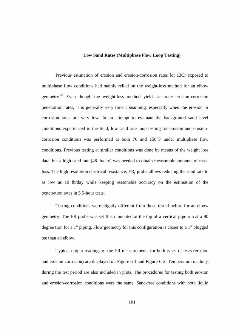
101
Low Sand Rates (Multiphase Flow Loop Testing)
Previous estimation of erosion and erosion-corrosion rates for 13Cr exposed to
multiphase flow conditions had mainly relied on the weight-loss method for an elbow
geometry.59 Even though the weight-loss method yields accurate erosion-corrosion
penetration rates, it is generally very time consuming, especially when the erosion or
corrosion rates are very low. In an attempt to evaluate the background sand level
conditions experienced in the field, low sand rate loop testing for erosion and erosion-
corrosion conditions was performed at both 76 and 150oF under multiphase flow
conditions. Previous testing at similar conditions was done by means of the weight loss
data, but a high sand rate (48 lb/day) was needed to obtain measurable amounts of mass
loss. The high resolution electrical resistance, ER, probe allows reducing the sand rate to
as low as 10 lb/day while keeping reasonable accuracy on the estimation of the
penetration rates in 5.5-hour tests.
Testing conditions were slightly different from those tested before for an elbow
geometry. The ER probe was set flush mounted at the top of a vertical pipe run at a 90
degree turn for a 1” piping. Flow geometry for this configuration is closer to a 1” plugged
tee than an elbow.
Typical output readings of the ER measurements for both types of tests (erosion
and erosion-corrosion) are displayed on Figure 6-1 and Figure 6-2. Temperature readings
during the test period are also included in plots. The procedures for testing both erosion
and erosion-corrosion conditions were the same. Sand-free conditions with both liquid

102
and gas phases flowing through the test cell were run long enough to stabilize system
temperature and metal loss readings. At least 1 hour of testing was conducted under
stable temperature conditions. During this period of the test, just the corrosion component
would cause a metal loss increment when a CO2-brine test is performed. However, no
measurable metal loss increments were observed in this period (sand-free) as shown by
the plateau for the first and last hour of erosion-corrosion testing shown in Figure 6-2.
This suggests that the pure corrosion component at tested conditions is very low,
probably below 1 mpy. After the initial, sand-free test period, dry sand was injected into
the system at the desired rate by means of a DC-motor driven vibratory sand feeder
system. Sand injection time is indicated on both Figure 6-1 and Figure 6-2 for pure
erosion and erosion-corrosion conditions, respectively. The sand was run for similar
times for both conditions (~5.5 hours) and then stopped. Later, the system was kept
running at sand-free conditions to again check the no-metal-loss increment response
under these conditions. Penetration rates were estimated from the slope of the metal-loss
vs. time plots. As can be observed at the end of the test shown in Figure 6-2, the metal-
loss output readings are pretty sensitive to changes in temperature. Once the temperature
was stable the metal loss noise level reduced to levels low enough to allow the
penetration rates to be measured with reasonable accuracy.
Some sharp spikes are observed in the output readings for both figures during the
stable temperature period. Notice that those spikes are caused by a sudden change in
temperature due to recharging of the condensed (colder) water back to the main liquid
tank separator from which the test cell is being fed. However, once the temperature
transients abated, the metal-loss reading returned back to similar previous values. This

103
few minutes transition period is not expected to affect the total slope much; therefore
spikes due to temperature transients were neglected in the estimation of the penetration
rates. The raw data was down-loaded to an Excel spread sheet and the changes in metal
loss due to changes in temperature were corrected before estimating the slope of the
metal-loss vs. time plots. Actually no large differences were found between spreadsheet
values and those provided by the commercial software.
y = 29.3x - 21.0pure E = 10.1 mpy
0
50
100
150
200
250
0 1 2 3 4 5 6 7 8Time (hr)
Met
alLo
ss(n
m)
0
20
40
60
80
100
120
140
160
Tem
po F
StartSand
StopSand
MetalLoss
Temperature
1” plugged T
Figure 6-1. Pure erosion test for 13Cr under sand-N2-distilled water flow system
(Vsg=60 ft/s, Vsl= 0.2 ft/s) at 150oF and low sand rate (15 lb/day).
The total thickness loss obtained for a low sand rate test was as low as 100 nm for
a 5.5-hour test. It is well known that the ER probes compensate for temperature effects.
However, at nanometer levels of precision, extremely small changes in temperature can
cause large changes in the output reading of the ER probe. Therefore, maintaining a
uniform sand rate during the 6-hour test at low levels of sand was also difficult to
achieve. Non-uniformity of sand rates during the 6-hour tests may be another source of
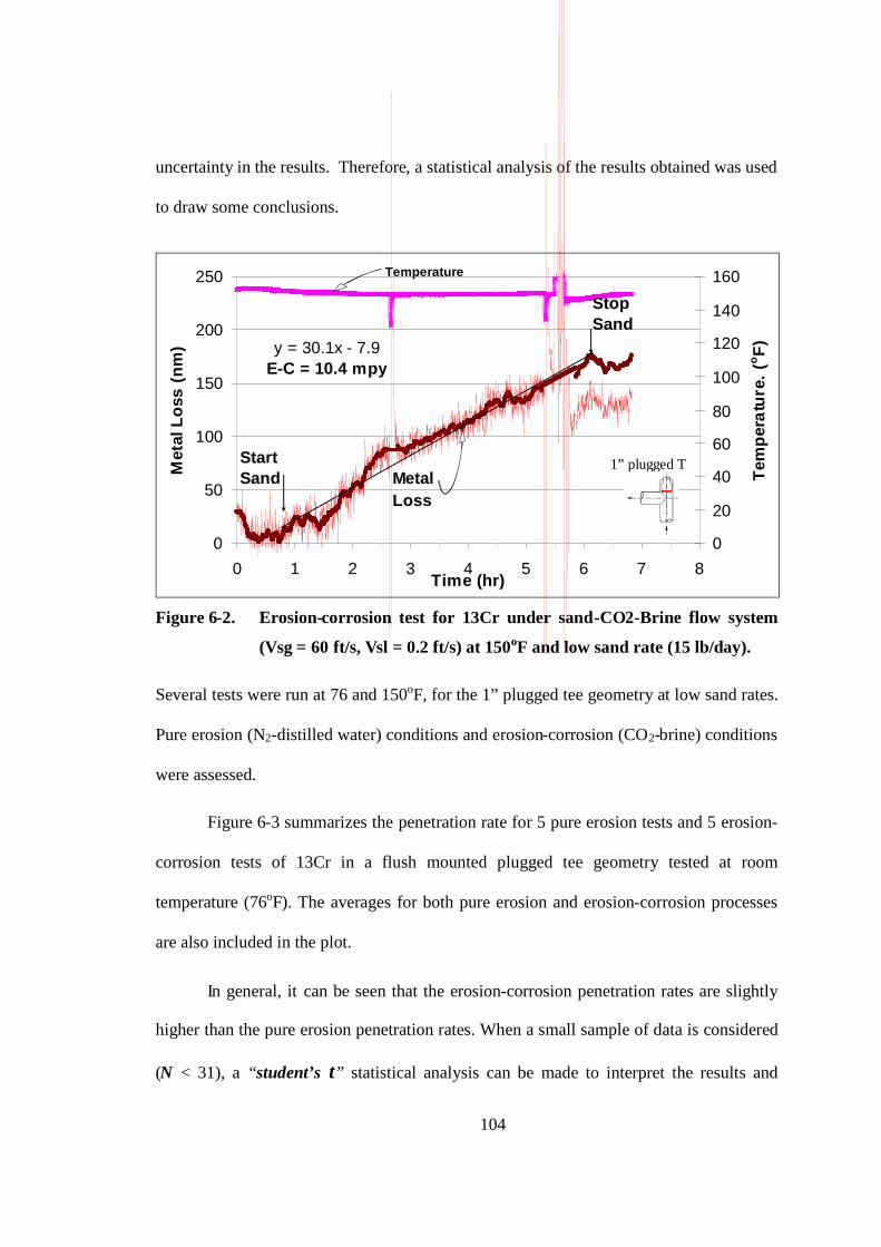
104
uncertainty in the results. Therefore, a statistical analysis of the results obtained was used
to draw some conclusions.
0
50
100
150
200
250
0 1 2 3 4 5 6 7 8Time (hr)
Met
alL
oss
(nm
)
0
20
40
60
80
100
120
140
160
Tem
per
atu
re.
(oF
)y = 30.1x - 7.9E-C = 10.4 mpy
StartSand
StopSand
MetalLoss
Temperature
1” plugged T
Figure 6-2. Erosion-corrosion test for 13Cr under sand-CO2-Brine flow system
(Vsg = 60 ft/s, Vsl = 0.2 ft/s) at 150oF and low sand rate (15 lb/day).
Several tests were run at 76 and 150oF, for the 1” plugged tee geometry at low sand rates.
Pure erosion (N2-distilled water) conditions and erosion-corrosion (CO2-brine) conditions
were assessed.
Figure 6-3 summarizes the penetration rate for 5 pure erosion tests and 5 erosion-
corrosion tests of 13Cr in a flush mounted plugged tee geometry tested at room
temperature (76oF). The averages for both pure erosion and erosion-corrosion processes
are also included in the plot.
In general, it can be seen that the erosion-corrosion penetration rates are slightly
higher than the pure erosion penetration rates. When a small sample of data is considered
(N < 31), a “student’s t” statistical analysis can be made to interpret the results and

105
estimate how well the obtained average is. A student’s t analysis to estimate the interval
within which the population average, X, will be contained approximately 95% of the time
was performed for both erosion and erosion-corrosion data. As can be noticed, the 95%
confidence intervals for both the erosion-corrosion average and the pure erosion average
overlap to a large extent. An additional F-distribution based analysis made on the data
shown in Figure 6-3, indicate with 95 % confidence that the erosion-corrosion rate is not
higher than the pure erosion rate. In any case the synergistic effect seen in previous
results conducted in an elbow geometry at higher sand rates was not observed for these
low sand rate data sets at 76oF.
0
1
2
3
4
5
Test #
Pen
etra
tion
rate
(mpy
)(E
Rpr
obe
)
E (mpy) 3.0 3.1 2.0 4.1 3.0 3.0
E-C (mpy) 3.1 4.6 3.9 3.5 3.0 3.6
1 2 3 4 5 Avg
Figure 6-3. Penetration rate for pure Erosion and Erosion-Corrosion tests of
13Cr in multiphase flow testing at 76oF. (The errors bars on the
average represent the 95% confidence interval on the mean value.)
Similar tests were also conducted at a higher temperature (150oF). To be able to
run similar tests at higher temperatures a minor modification of the sand feeder was

106
made. The clear PVC pipe used in the sand feeder system to introduce the dry sand into
the flow-stream was change to a stainless steel pipe. The sand bed on this pipe was no
longer visible, therefore the sand rates were increased a little (from 10 to 15 lb/day
approximately) to ensure sand flow into the system.
Figure 6-4 summarizes the penetration rate for 3 pure erosion tests and 3 erosion-
corrosion tests of 13Cr in a flush mounted plugged tee geometry tested at 150oF and 15
lb/day. The averages for both pure erosion and erosion-corrosion processes are also
included in the plot, as well as the 95% confidence interval error bars. As can be seen, the
scatter of the pure erosion data set of the 150oF data was higher than the scatter found for
the remaining of the data sets. Additionally the number of tests run was lower than the
number of the test run at 76oF which makes the uncertainty of these results larger.
However, similar trends as obtained for 76oF can be seen for 150oF as well. The erosion-
corrosion penetration rates are slightly higher than the pure erosion penetration rates. But
if there is an erosion-corrosion synergistic effect for this temperature at low sand rate
conditions, it is not very significant.
Care must be taken when scaling up the flow loop test results to extrapolate them
to field conditions. Spatial distribution or density of sand over the cross section needs to
be considered to evaluate how erosive a specific condition may be. A sand rate of 10
lb/day represents a sand mass flux of about 12 lb/day-in2 for the 1” piping used in our
tests. By contrast, the same sand mass flux would represent a sand mass rate of about 89,
153 and 600 lb/day for 3”, 4” and 8” pipes diameter (schedule 40) respectively. Or, in
other words, a sand rate of 10 lb/day, which represents a sand flux of about 12 lb/day-in2
107
in 1” piping, would represent sand fluxes of only about 1.4, 0.8 and 0.2 lb/day-in2 for 3”,
4” and 8” pipes diameter (schedule 40) respectively.
This analysis suggests that erosivities for laboratory flow loop tests conducted at
low sand rates may still be considered more aggressive than those seen in field at
“background sand levels” conditions. Hence, in light of the laboratory results, no
significant erosion-corrosion synergistic effect of 13Cr is expected for low erosivity
conditions for either 76 or 150oF.
0
2
4
6
8
10
12
14
16
Pen
etra
tion
rate
(mp
y)(E
Rp
rob
e)
E (mpy) 10.1 7.2 5.0 7.4
E-C (mpy) 10.4 8.8 11.0 10.0
1 2 3 AvgTest #
Figure 6-4. Penetration rate for pure Erosion and Erosion-Corrosion tests of 13Cr
in multiphase flow testing at 150oF. (The errors bars on the average
represent the 95% confidence interval on the mean value.)

108
High Sand Rates (Multiphase Flow Loop Testing)
A set of multiphase flow loop tests for 13Cr, Super 13Cr and 22Cr at high
erosivity conditions was also performed. High resolution electrical resistant probes made
of the three CRAs under study were obtained and used in a gas/liquid/sand flow facility
to measure pure erosion rates and erosion-corrosion rates. For these sets of testing a
special fitting was use to configure the ER probes in a ½” pipe test section for the
multiphase flow loop. With the new arrangement, the same plugged tee flow geometry as
used for low sand rate experiments was tested, but now the clearance between the
cylindrical probe and the ½” piping was much smaller than the one between the probe
and the 1” piped test section used before. Hence, using the ½” pipe system assured that
the probe would be directly exposed to the impingement of the entire sand through put,
obtaining much higher erosivity conditions than those for the 1” geometry. In addition, a
much higher sand flux was used for the high sand rate testing (30-99 lb/day-in2 for the ½”
pipe) as compared to the low sand rate testing (10-12 lb/day-in2 for the 1” pipe).
Therefore, as far as sand concentration is concerned, the “high sand rate” erosivities were
10 times more aggressive than the “low sand rate” erosivities. However, flow conditions
also were different. A superficial gas velocity of 20ft/s and superficial liquid velocity of
1.4 ft/s were used for the ½” pipe tests and superficial gas velocity of 60ft/s and
superficial liquid velocity of 0.2 ft/s were used for the 1” pipe tests, both conditions were
annular flow.
The testing procedure was similar to that used for determination of erosion-
corrosion of 13Cr alloy under low sand concentration presented in the previous section.

109
Hence, the output reading trends of the ER measurements for both types of tests (erosion
and erosion-corrosion) are similar to those displayed on Figure 6-1 and Figure 6-2 in the
previous section, even though the magnitudes of slopes, and thus the erosion and erosion-
corrosion rates were much higher.
Table 6-1 contains the pure erosion and erosion-corrosion penetration rates for the
three alloys tested at similar conditions (76oF, pH 4, Vsg = 20 ft/s, Vsl = 1.4 ft/s, 30 lb/day
of sand). The total corrosion component rates, Ce-c of the erosion-corrosion process, were
estimated by subtracting the pure erosion rates, E from the total erosion-corrosion rates
EC. Trends found are as expected. In general the erosion-corrosion rates were higher than
the pure erosion rate for each of the three materials. Considering that the pure corrosion
rates for these alloys have been proved to be smaller than 2 mpy at the conditions tested,
the current results suggest that a synergistic effect is observed in the erosion-corrosion
processes of the three alloys, provided that the erosivity is high enough. However, the
degree of synergism is quite different for the three alloys: at the much lower sand rates
typically found in the field, the synergism could be negligible for 22Cr, or at least never
observed in the field.
The ratio of EC to pure erosion (E) for 13Cr was the highest, with a value of 2.2
followed by Super 13Cr at 1.6 and 22Cr at 1.4. Slight differences, if any, were seen in the
pure erosion penetration rates between the three alloys, which may fall within the
reproducibility errors of the measurements. Unfortunately, due to lack of time and
resources, a rigorous reproducibility procedure was not followed this time as in previous
data sets. However experience gathered by running the multiphase flow loop and the ER
probes for similar testing procedures has shown the 95% confidence interval of the

110
penetration rate estimation falling within 10 to 30% of the mean value. If the worst case
scenario (30%) is adopted for data shown in Table 6-1, one may get a sense of whether
the erosion-corrosion rate is higher than pure erosion rates for a given condition. Figure
6-5 shows data from Table 6-1 including the assumed error interval of 30%. This plot
strongly suggests that the erosion-corrosion rate is higher than the pure erosion rate for
13Cr at 76oF. For super13Cr this effect is less pronounced, and for 22Cr may not be
significant. Notice, for 13Cr, the corrosion component is even higher than the pure
erosion for what may be defined as corrosion dominated erosion-corrosion process.
Erosion and erosion-corrosion data were also gathered for the 3 alloys exposed to
similar flow conditions but a higher temperature of 150oF (see Table 6-2, and Figure 6-6).
In general, trends found at 150oF are similar to those observed at 76oF. A point to
highlight is that the corrosion component of the Super13Cr, which was lower than the
pure erosion rate at 76oF, is higher than the pure erosion rate at 150oF; hence, at this
temperature the erosion-corrosion to erosion ratio is significant for Super13Cr as it is for
13Cr. For 22Cr, erosion-corrosion rates and erosion-corrosion to erosion ratios are low
and quite similar regardless of the temperature. Meaning the repassivation rates are not
strongly affected by the temperature, as was also seen in scratch test results obtained for
this alloy in Chapter 5.

111
Table 6-1. Erosion-corrosion (EC), pure erosion (E) and corrosion components
(Ce-c) of the erosion-corrosion penetration rates for 3 alloys tested atsimilar conditions. 76oF, pH 4, Vsg = 20 ft/s, Vsl = 1.4 ft/s, 30 lb/day of
sand.
Alloy
EC rate (mpy)
ER Probe
E rate (mpy)
ER Probe
Ce-c rate (mpy)
*Ce-c =EC- E
13Cr 179 80 99
Super 13Cr 123 76 47
22Cr 95 66 29
*Obtained by subtracting the pure erosion from the total erosion-corrosion.
Figure 6-5. Erosion-corrosion (EC), pure erosion (pure E) and corrosion
component (CEC) of the erosion-corrosion penetration rates for data
shown in Table 6-1.
0
50
100
150
200
250
13Cr alloy Super13Cr alloy 22Cr alloyMaterial
Pene
trat
ion
rate
(mp
y)
ER Probeflush mounted
1/2" plugged tee
76oF
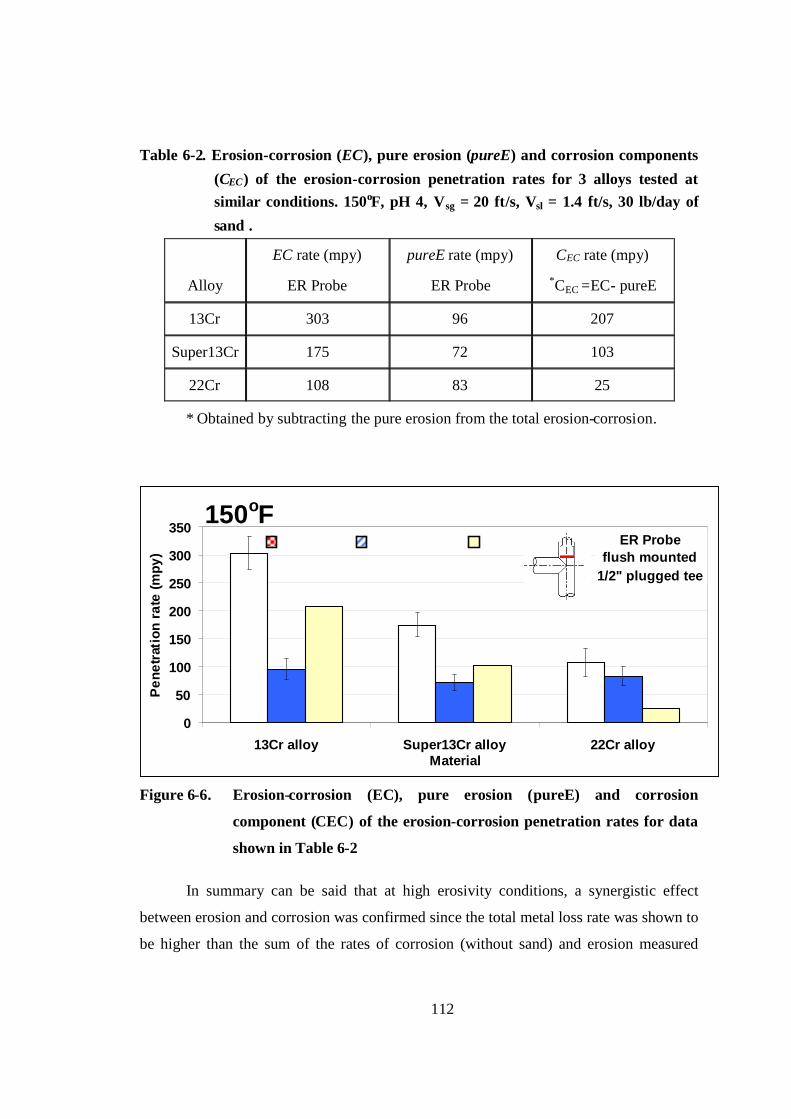
112
Table 6-2. Erosion-corrosion (EC), pure erosion (pureE) and corrosion components
(CEC) of the erosion-corrosion penetration rates for 3 alloys tested atsimilar conditions. 150oF, pH 4, Vsg = 20 ft/s, Vsl = 1.4 ft/s, 30 lb/day of
sand .
Alloy
EC rate (mpy)
ER Probe
pureE rate (mpy)
ER Probe
CEC rate (mpy)
*CEC =EC- pureE
13Cr 303 96 207
Super13Cr 175 72 103
22Cr 108 83 25
* Obtained by subtracting the pure erosion from the total erosion-corrosion.
Figure 6-6. Erosion-corrosion (EC), pure erosion (pureE) and corrosion
component (CEC) of the erosion-corrosion penetration rates for data
shown in Table 6-2
In summary can be said that at high erosivity conditions, a synergistic effect
between erosion and corrosion was confirmed since the total metal loss rate was shown to
be higher than the sum of the rates of corrosion (without sand) and erosion measured
0
50
100
150
200
250
300
350
13Cr alloy Super13Cr alloy 22Cr alloyMaterial
Pen
etra
tion
rate
(mpy
)
ER Probeflush mounted
1/2" plugged tee
150oF

113
separately. It appears that under the high sand rate conditions tested, the erosivity is
severe enough to damage the passive layer thereby enhancing the corrosion rate.
Synergism seems to occur for the three alloys; however, the degree of synergism is quite
different for the three alloys and may not be significant for 22Cr under field conditions
where erosivities are typically much lower that those occurring in the small bore loop
used in this testing.
For the other two alloys, 13Cr and Super13Cr, especially at high temperatures, if
the erosion rate of the passive film is great enough, then an accelerated erosion-corrosion
process may take place with a significant contribution from a corrosion component.

114
CHAPTER 7
COMPARISON OF SCRATCH TEST RESULTS WITH FLOW LOOP
TEST RESULTS
An expression to estimate the corrosion component of the erosion corrosion, Ce-c
for the conditions being studied has not been yet constructed, however, information
generated with the scratch test cell method presented in Chapter 5 may provide the basis
for a procedure intended to predict the corrosion component, Ce-c of CRAs exposed to
environments containing CO2 and sand.
This section compares some of the trends obtained from scratch test results with
loop test data assuming that the scratch test results relate to the total corrosion component
of the erosion-corrosion process caused by the scratch (e.g. Ce-c). This suggests that the
scratch test results should be comparable to the estimation of the “total corrosion” in a
loop test conducted under CO2-brine-sand flow conditions, where the “total corrosion”
component is the summation of the pure corrosion (sand-free corrosion) and the corrosion
increment induced by the sand impingement process.
Hence, the scratch test data is being compared here to the single phase liquid flow
loop data presented in previous publications57,58 for 13Cr alloy, as well as to the two-
phase flow loop data gathered for 13Cr, Super13Cr and 22Cr and presented in Chapter 6.
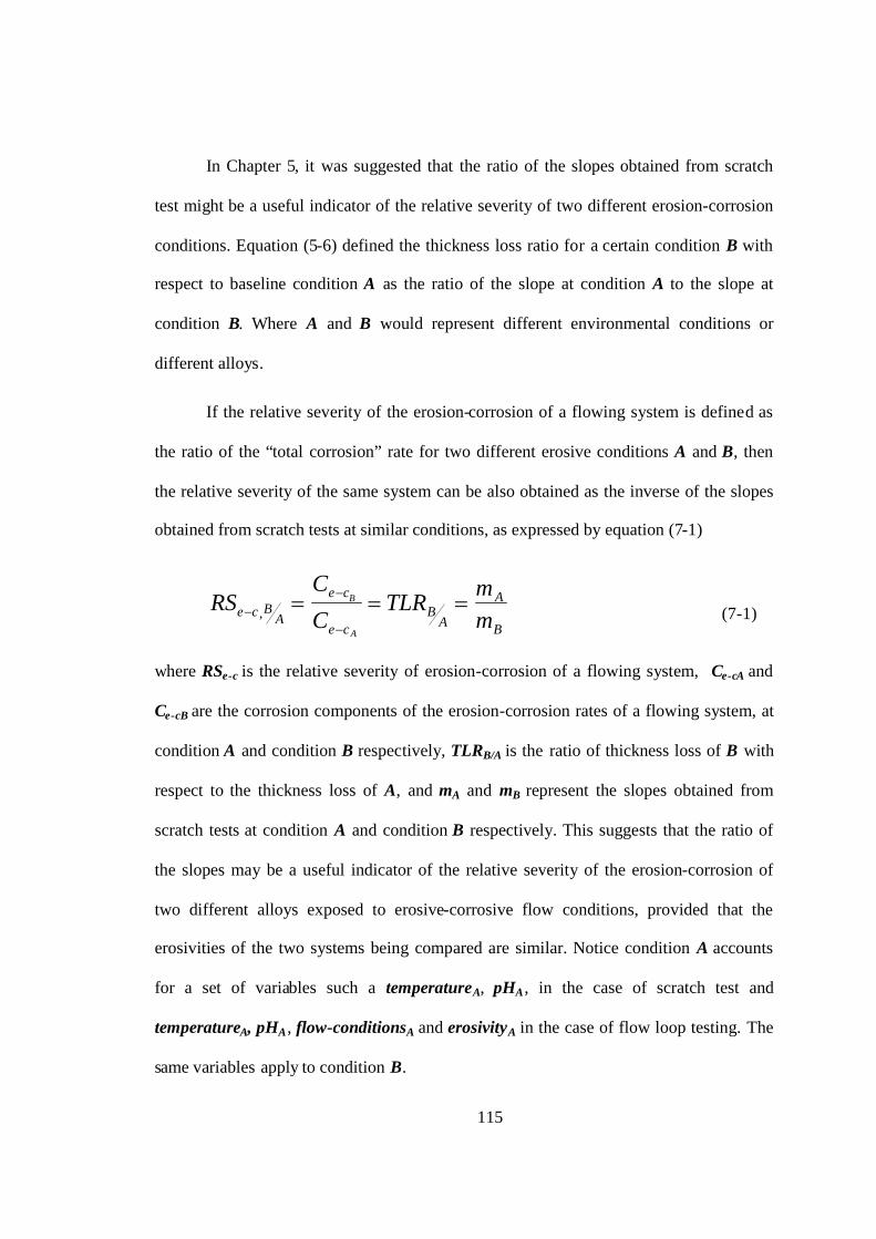
115
In Chapter 5, it was suggested that the ratio of the slopes obtained from scratch
test might be a useful indicator of the relative severity of two different erosion-corrosion
conditions. Equation (5-6) defined the thickness loss ratio for a certain condition B with
respect to baseline condition A as the ratio of the slope at condition A to the slope at
condition B. Where A and B would represent different environmental conditions or
different alloys.
If the relative severity of the erosion-corrosion of a flowing system is defined as
the ratio of the “total corrosion” rate for two different erosive conditions A and B, then
the relative severity of the same system can be also obtained as the inverse of the slopes
obtained from scratch tests at similar conditions, as expressed by equation (7-1)
B
A
AB
ce
ce
ABce m
mTLR
C
CRS
A
B
, (7-1)
where RSe-c is the relative severity of erosion-corrosion of a flowing system, Ce-cA and
Ce-cB are the corrosion components of the erosion-corrosion rates of a flowing system, at
condition A and condition B respectively, TLRB/A is the ratio of thickness loss of B with
respect to the thickness loss of A, and mA and mB represent the slopes obtained from
scratch tests at condition A and condition B respectively. This suggests that the ratio of
the slopes may be a useful indicator of the relative severity of the erosion-corrosion of
two different alloys exposed to erosive-corrosive flow conditions, provided that the
erosivities of the two systems being compared are similar. Notice condition A accounts
for a set of variables such a temperatureA, pHA, in the case of scratch test and
temperatureA, pHA, flow-conditionsA and erosivityA in the case of flow loop testing. The
same variables apply to condition B.
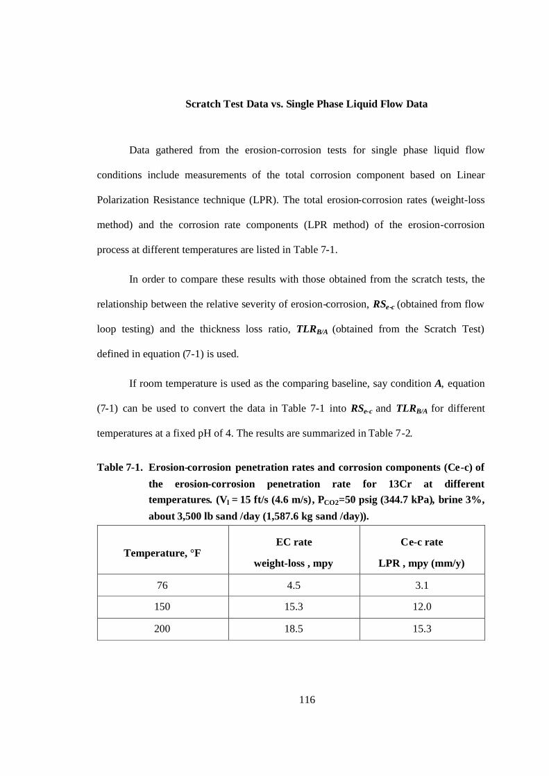
116
Scratch Test Data vs. Single Phase Liquid Flow Data
Data gathered from the erosion-corrosion tests for single phase liquid flow
conditions include measurements of the total corrosion component based on Linear
Polarization Resistance technique (LPR). The total erosion-corrosion rates (weight-loss
method) and the corrosion rate components (LPR method) of the erosion-corrosion
process at different temperatures are listed in Table 7-1.
In order to compare these results with those obtained from the scratch tests, the
relationship between the relative severity of erosion-corrosion, RSe-c (obtained from flow
loop testing) and the thickness loss ratio, TLRB/A (obtained from the Scratch Test)
defined in equation (7-1) is used.
If room temperature is used as the comparing baseline, say condition A, equation
(7-1) can be used to convert the data in Table 7-1 into RSe-c and TLRB/A for different
temperatures at a fixed pH of 4. The results are summarized in Table 7-2.
Table 7-1. Erosion-corrosion penetration rates and corrosion components (Ce-c) of
the erosion-corrosion penetration rate for 13Cr at differenttemperatures. (Vl = 15 ft/s (4.6 m/s), PCO2=50 psig (344.7 kPa), brine 3%,
about 3,500 lb sand /day (1,587.6 kg sand /day)).
Temperature, °FEC rate
weight-loss , mpy
Ce-c rate
LPR , mpy (mm/y)
76 4.5 3.1
150 15.3 12.0
200 18.5 15.3
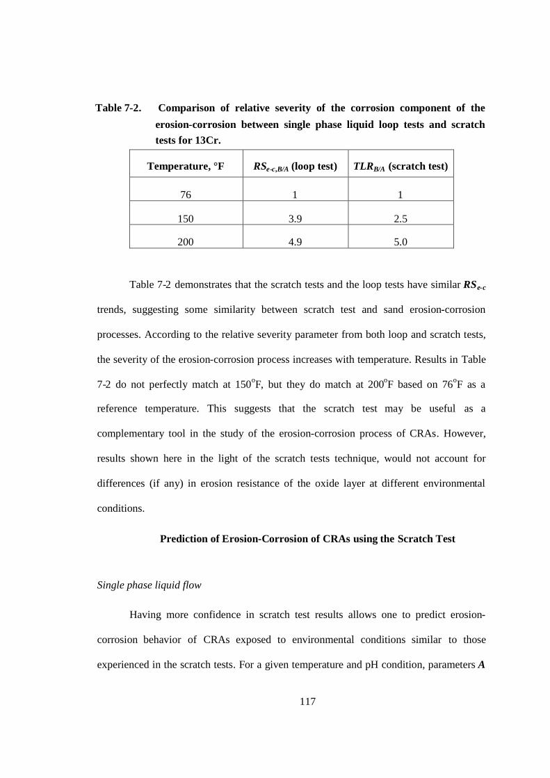
117
Table 7-2. Comparison of relative severity of the corrosion component of the
erosion-corrosion between single phase liquid loop tests and scratchtests for 13Cr.
Temperature, °F RSe-c,B/A (loop test) TLRB/A (scratch test)
76 1 1
150 3.9 2.5
200 4.9 5.0
Table 7-2 demonstrates that the scratch tests and the loop tests have similar RSe-c
trends, suggesting some similarity between scratch test and sand erosion-corrosion
processes. According to the relative severity parameter from both loop and scratch tests,
the severity of the erosion-corrosion process increases with temperature. Results in Table
7-2 do not perfectly match at 150oF, but they do match at 200oF based on 76oF as a
reference temperature. This suggests that the scratch test may be useful as a
complementary tool in the study of the erosion-corrosion process of CRAs. However,
results shown here in the light of the scratch tests technique, would not account for
differences (if any) in erosion resistance of the oxide layer at different environmental
conditions.
Prediction of Erosion-Corrosion of CRAs using the Scratch Test
Single phase liquid flow
Having more confidence in scratch test results allows one to predict erosion-
corrosion behavior of CRAs exposed to environmental conditions similar to those
experienced in the scratch tests. For a given temperature and pH condition, parameters A
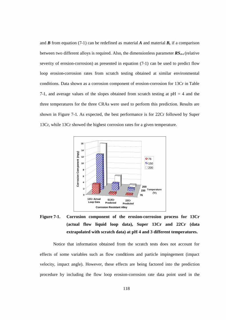
118
and B from equation (7-1) can be redefined as material A and material B, if a comparison
between two different alloys is required. Also, the dimensionless parameter RSe-c (relative
severity of erosion-corrosion) as presented in equation (7-1) can be used to predict flow
loop erosion-corrosion rates from scratch testing obtained at similar environmental
conditions. Data shown as a corrosion component of erosion-corrosion for 13Cr in Table
7-1, and average values of the slopes obtained from scratch testing at pH = 4 and the
three temperatures for the three CRAs were used to perform this prediction. Results are
shown in Figure 7-1. As expected, the best performance is for 22Cr followed by Super
13Cr, while 13Cr showed the highest corrosion rates for a given temperature.
13Cr ActualLoop Data
S13CrPredicted
22CrPredicted
76
150200
0
2
4
6
8
10
12
14
16
Cor
rosi
onC
ompo
nent
(mpy
)
Corrosion Resistant Alloy
Temperature(oF)
76
150200
Figure 7-1. Corrosion component of the erosion-corrosion process for 13Cr
(actual flow liquid loop data), Super 13Cr and 22Cr (data
extrapolated with scratch data) at pH 4 and 3 different temperatures.
Notice that information obtained from the scratch tests does not account for
effects of some variables such as flow conditions and particle impingement (impact
velocity, impact angle). However, these effects are being factored into the prediction
procedure by including the flow loop erosion-corrosion rate data point used in the

119
equation (7-1). The procedure requires that the flow and erosivity conditions to which
EC-predicted alloys (Super 13Cr and 22Cr in this example case) are assumed to be
exposed, are the same conditions to which the reference alloy (13Cr in this example case)
was exposed in the flow loop test. Furthermore, the procedure assumes, that differences
in the erosion responses of the different alloys are negligible as compared to the effects
that environmental conditions such as pH and temperature have in the total erosion-
corrosion process. In other words, differences in the erosion damage in the different
alloys here tested are assumed to be small provided the alloys are all exposed to similar
flow and erosivity conditions (sand concentration, sand size and shape).
Validation of Scratch Test Predictions of Erosion-Corrosion of CRAs
Multiphase flow
In general, predictions of the corrosion component of erosion-corrosion based on
scratch test data compared well to test results from multiphase gas/liquid flow loop for
the three CRAs at high erosivity conditions. Hence, second order behavior appears to be
an appropriate and useful model to represent the repassivation process of CRAs. A
procedure to predict penetration rates for erosion-corrosion conditions was developed
based on this second order model behavior observed by the re-healing process of the
passive film of CRAs under tested conditions. The procedure, as developed thus far,
requires that one flow loop test be run at known environmental conditions and specified
flow and erosivity conditions Once the erosion-corrosion rate for this baseline set of
conditions is established, then, provided erosivity conditions remain unchanged, erosion-
corrosion rates can be predicted for other environments and other CRAs for which

120
scratch test data is available. Good agreement between the actual and predicted
penetration rates was found.
Table 7-3 shows actual and predicted values of the corrosion component (Ce-c) of
the erosion-corrosion penetration rates for 3 alloys tested at similar conditions (76oF and
pH = 4). Actual values are the same as displayed in Table 6-1 of Chapter 6. Predicted
values were obtained by mean of equation (7-1) and the slope ratio of the scratch test data
using 13Cr loop data as a reference (A) material. As can be seen, actual and predicted Ce-c
values match very well, suggesting scratch test data may be useful for predicting erosion-
corrosion penetration rates provided that data from at least one loop test is available.
An analysis similar to that done for the penetration rates of the three CRAs at
room temperature can be done for 150oF with flow loop test data shown in Table 6-2 of
Chapter 6 and proper used of the slopes obtained by means of scratch tests. Results of
this comparison are shown in Table 7-4. In general, trends found at 150oF are similar to
those observed at 76oF. Notice that the scratch test prediction data seem to closely match
the trends and observations obtained from loop test data.
In general, predictions of the corrosion component of erosion-corrosion based on
scratch test data compared well to test results from multiphase gas/liquid flow loop for
the three CRAs at high erosivity conditions. Hence, second order behavior appears to be
an appropriate and useful model to represent the repassivation process of CRAs. A
procedure to predict penetration rates for erosion-corrosion conditions was developed
based on this second order model behavior observed by the re-healing process of the
passive film of CRAs under tested conditions. The procedure, as developed thus far,
requires that one flow loop test be run at known environmental conditions and specified

121
flow and erosivity conditions Once the erosion-corrosion rate for this baseline set of
conditions is established, then, provided erosivity conditions remain unchanged, erosion-
corrosion rates can be predicted for other environments and other CRAs for which
scratch test data is available. Good agreement between the actual and predicted
penetration rates was found.
Table 7-3. Actual and predicted values of the corrosion component (Ce-c) of the
erosion-corrosion penetration rates for 3 alloys tested at similar
conditions (76oF, pH 4)
Alloy
Actual Ce-crate
*Ce-c =EC- E
(mpy)
Scratch Test Data
TLRB/A =(m13Cr/mCRA)
Predicted Ce-c rate
Ce-c,CRA= TLRB/A CEC, 13Cr
(mpy)
13Cr 99 1 (reference)
Super13Cr 47 0.40 40
22Cr 29 0.22 22
*Obtained from subtraction the erosion from the erosion-corrosion
Table 7-4. Actual and predicted values of the corrosion component (CEC) of theerosion-corrosion penetration rates for 3 alloys tested at similar
conditions (150oF, pH 4).
Alloy
Actual CEC rate
*Ce-c =EC- E
(mpy)
Scratch Test Data
TLRB/A =(m13Cr/mCRA)
Predicted Ce-c rate
Ce-c,CRA= TLRB/A CEC, 13Cr
(mpy)
13Cr 207 1 (reference)
Super13Cr 103 0.34 71
22Cr 25 0.12 25
* Obtained from subtraction the erosion from the erosion-corrosion

122
CHAPTER 6 ................................................................................................................................100
MULTIPHASE GAS/LIQUID/SAND FLOW LOOP TESTING RESULTS................................................100
Low Sand Rates (Multiphase Flow Loop Testing)................................ ...............................101
High Sand Rates (Multiphase Flow Loop Testing)..............................................................108
CHAPTER 7 ................................................................................................................................114
COMPARISON OF SCRATCH TEST RESULTS WITH FLOW LOOP TEST RESULTS ..............................114
Scratch test data vs. single phase liquid flow data ..............................................................116
Prediction of Erosion-Corrosion of CRAs using the Scratch Test.......................................117
Single phase liquid flow.......................................................................................................................117
Validation of Scratch Test Predictions of Erosion-Corrosion of CRAs...............................119
Multiphase flow....................................................................................................................................119

123
TABLE 6-1. EROSION-CORROSION (EC), PURE EROSION (E) AND CORROSION COMPONENTS (CE-C) OF THE
EROSION-CORROSION PENETRATION RATES FOR 3 ALLOYS TESTED AT SIMILAR CONDITIONS. 76OF, PH 4,
VSG = 20 FT/S, VSL = 1.4 FT/S, 30 LB/DAY OF SAND...............................................................................111
TABLE 6-2. EROSION-CORROSION (EC), PURE EROSION (PUREE) AND CORROSION COMPONENTS (CEC) OF THE
EROSION-CORROSION PENETRATION RATES FOR 3 ALLOYS TESTED AT SIMILAR CONDITIONS. 150OF, PH
4, VSG = 20 FT/S, VSL = 1.4 FT/S, 30 LB/DAY OF SAND . ................................................................ .........112
TABLE 7-1. EROSION-CORROSION PENETRATION RATES AND CORROSION COMPONENTS (CE-C) OF THE
EROSION-CORROSION PENETRATION RATE FOR 13CR AT DIFFERENT TEMPERATURES. (VL = 15 FT/S (4.6
M/S), PCO2=50 PSIG (344.7 KPA), BRINE 3%, ABOUT 3,500 LB SAND /DAY (1,587.6 KG SAND /DAY))..116
TABLE 7-2. COMPARISON OF RELATIVE SEVERITY OF THE CO RROSION COMPONENT OF THE EROSION-
CORROSION BETWEEN SINGLE PHASE LIQUID LOOP TESTS AND SCRATCH TESTS FOR 13CR. ................117
TABLE 7-3. ACTUAL AND PREDICTED VALUES OF THE CORROSION COMPONENT (CE-C) OF THE EROSION-
CORROSION PENETRATION RATES FOR 3 ALLOYS TESTED AT SIMILAR CONDITIONS (76OF, PH 4) ........120
TABLE 7-4. ACTUAL AND PREDICTED VALUES OF THE CORROSION COMPONENT (CEC) OF THE EROSION-
CORROSION PENETRATION RATES FOR 3 ALLOYS TESTED AT SIMILAR CONDITIONS (150OF, PH 4). .....121
FIGURE 6-1. PURE EROSION TEST FOR 13CR UNDER SAND-N2-DISTILLED WATER FLOW SYSTEM (VSG=60
FT/S, VSL= 0.2 FT/S) AT 150OF AND LOW SAND RATE (15 LB/DAY). ................................ ......................103
FIGURE 6-2. EROSION-CORROSION TEST FOR 13CR UNDER SAND-CO2-BRINE FLOW SYSTEM (VSG=60 FT/S,
VSL= 0.2 FT/S) AT 150OF AND LOW SAND RATE (15 LB/DAY). ................................ .............................104
FIGURE 6-3. PENETRATION RATE FOR PURE EROSION AND EROSION-CORROSION TESTS OF 13CR IN
MULTIPHASE FLOW TESTING AT 76OF. (THE ERRORS BARS ON THE AVERAGE REPRESENT THE 95%
CONFIDENCE INTERVAL ON THE MEAN VALUE.) ................................................................ ..................105
FIGURE 6-4. PENETRATION RATE FOR PURE EROSION AND EROSION-CORROSION TESTS OF 13CR IN
MULTIPHASE FLOW TESTING AT 150OF. (THE ERRORS BARS ON THE AVERAGE REPRESENT THE 95%
CONFIDENCE INTERVAL ON THE MEAN VALUE.) ................................................................ ..................107
FIGURE 6-5. EROSION-CORROSION (EC), PURE EROSION (PURE E) AND CORROSION COMPONENT (CEC) OF
THE EROSION-CORROSION PENETRATION RATES FOR DATA SHOWN IN TABLE 6-1...............................111
FIGURE 6-6. EROSION-CORROSION (EC), PURE EROSION (PUREE) AND CORROSION COMPONENT (CEC)
OF THE EROSION-CORROSION PENETRATION RATES FOR DATA SHOWN IN TABLE 6-2..........................112
FIGURE 7-1. CORROSION COMPONENT OF THE EROSION-CORROSION PROCESS FOR 13CR (ACTUAL FLOW
LIQUID LOOP DATA), SUPER13CR AND 22CR (DATA EXTRAPOLATED WITH SCRATCH DATA) AT PH 4
AND 3 DIFFERENT TEMPERATURES. .....................................................................................................118

124
59 Rincon, H.E. (2001). "Erosion-Corrosion Phenomena of 13Cr Alloy in Flows
Containing Sand Particles". M.S. Thesis, Department of Mechanical Engineering, TheUniversity of Tulsa, Ok, Tulsa..
57 Rincon, H.E., Chen, J. and Shadley, J.R. (2002). "Erosion-Corrosion Phenomenaof 13Cr Alloy in Flows Containing Sand Particles". Corrosion/2002, paper no.2493, (Houston, TX, USA, NACE International.
58 Chen, J., Shadley, J.R., Rincon, H.E. and Rybicki, E.F. (2003). "Effects ofTemperature on Erosion-Corrosion of 13Cr". Corrosion/2003, paper no. 3320,(Houston, TX, USA, NACE International.

122
CHAPTER 8
SUBMERGED DIRECT IMPINGEMENT TEST: SINGLE PHASE LIQUID
FLOW
Erosion-Corrosion Liquid/Sand Loop (Microloop)
The study of the effects of some environmental parameters (temperature and pH)
on the repassivation behavior of CRAs in CO2-saturated brine was extensively discussed
in Chapter 5. This study was performed based on results obtained with the “Scratch
Test”60, a laboratory method conducted in a glass cell. Some similarities between the
scratch test and the sand erosion process observed in pipe-flow conditions have been
previously mentioned as well. The convenience of the experimental setup used for the
scratch test to separate the mechanical process (mechanical removal of material) from the
electrochemical process (corrosion) during repassivation of CRAs has been mentioned.
However, in the sand erosion-corrosion process, the mechanical and electrochemical
processes involved take place simultaneously and continuously during impingement of
solid particles on the target material. Thus, prediction of erosion-corrosion needs to
account for parameters driven by flow field conditions such as flow velocity, flow
geometry and sand rate. For this purpose, a single phase liquid flow loop was used to

123
experimentally determine the effect of flow velocity and sand rate in the erosion-
corrosion mechanism of CRAs.
Data were collected based on an electrochemical technique. The instrumentation
and the configuration of the electrodes used for scratch test were successfully adapted to
the dynamic flow loop testing as described in Chapter 4. Thus, the working electrode
(target specimen) is continuously impinged by sand particles while the potential and
current are recorded.
The main objective of the flow loop testing was to check the effect of certain
parameters such a flow velocity and sand rate on the repassivation behavior of CRAs.
Data collected in the flow loop testing also provided a reference point and target to the
predictions of erosion rates (E), corrosion component rates (Ce-c), and total erosion-
corrosion rates (E-C).
However, obtaining quality data with the low erosivities commonly obtained in
liquid flows testing is challenging and time consuming, if the weight loss technique is
used. Thus, several electrochemical techniques along with a few weight loss tests were
performed
The set of electrochemical tests conducted are based upon the response of the
current flowing between two electrodes made of the same CRA but exposed to different
flow conditions. The working electrode #1 is the target specimen exposed to the sand
laden impinging jet. A larger auxiliary working electrode #2, is placed upstream of the
nozzle and thus is not exposed to the flowing sand at any time during the test. Other
standard electrochemical techniques, such as LPR and potentio-dynamic scans, were also
performed at selected conditions.
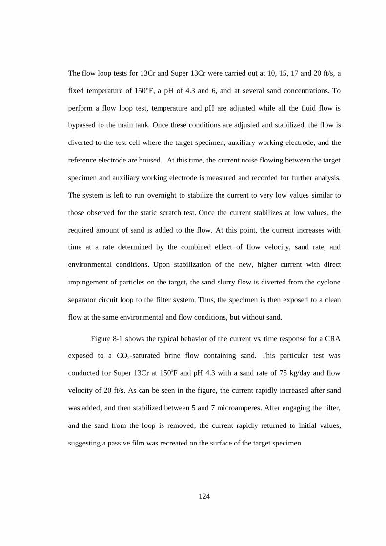
124
The flow loop tests for 13Cr and Super 13Cr were carried out at 10, 15, 17 and 20 ft/s, a
fixed temperature of 150°F, a pH of 4.3 and 6, and at several sand concentrations. To
perform a flow loop test, temperature and pH are adjusted while all the fluid flow is
bypassed to the main tank. Once these conditions are adjusted and stabilized, the flow is
diverted to the test cell where the target specimen, auxiliary working electrode, and the
reference electrode are housed. At this time, the current noise flowing between the target
specimen and auxiliary working electrode is measured and recorded for further analysis.
The system is left to run overnight to stabilize the current to very low values similar to
those observed for the static scratch test. Once the current stabilizes at low values, the
required amount of sand is added to the flow. At this point, the current increases with
time at a rate determined by the combined effect of flow velocity, sand rate, and
environmental conditions. Upon stabilization of the new, higher current with direct
impingement of particles on the target, the sand slurry flow is diverted from the cyclone
separator circuit loop to the filter system. Thus, the specimen is then exposed to a clean
flow at the same environmental and flow conditions, but without sand.
Figure 8-1 shows the typical behavior of the current vs. time response for a CRA
exposed to a CO2-saturated brine flow containing sand. This particular test was
conducted for Super 13Cr at 150oF and pH 4.3 with a sand rate of 75 kg/day and flow
velocity of 20 ft/s. As can be seen in the figure, the current rapidly increased after sand
was added, and then stabilized between 5 and 7 microamperes. After engaging the filter,
and the sand from the loop is removed, the current rapidly returned to initial values,
suggesting a passive film was recreated on the surface of the target specimen
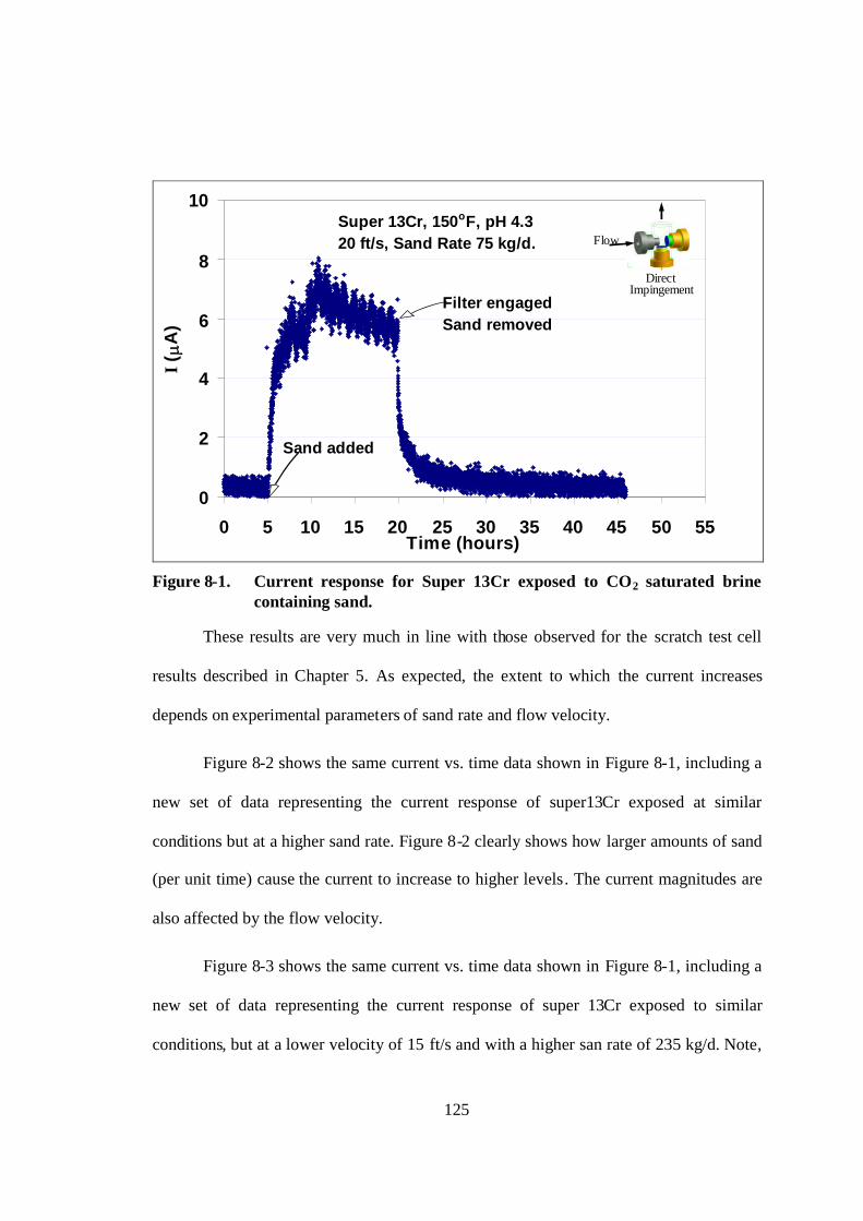
125
0
2
4
6
8
10
0 5 10 15 20 25 30 35 40 45 50 55Time (hours)
I( m
A)
Super 13Cr, 150oF, pH 4.320 ft/s, Sand Rate 75 kg/d.
Sand added
Filter engagedSand removed
Flow
ImpingementDirect
Figure 8-1. Current response for Super 13Cr exposed to CO2 saturated brinecontaining sand.
These results are very much in line with those observed for the scratch test cell
results described in Chapter 5. As expected, the extent to which the current increases
depends on experimental parameters of sand rate and flow velocity.
Figure 8-2 shows the same current vs. time data shown in Figure 8-1, including a
new set of data representing the current response of super13Cr exposed at similar
conditions but at a higher sand rate. Figure 8-2 clearly shows how larger amounts of sand
(per unit time) cause the current to increase to higher levels. The current magnitudes are
also affected by the flow velocity.
Figure 8-3 shows the same current vs. time data shown in Figure 8-1, including a
new set of data representing the current response of super 13Cr exposed to similar
conditions, but at a lower velocity of 15 ft/s and with a higher san rate of 235 kg/d. Note,
126
that the current data series for 15 ft/s (235 kg/day) stabilized at lower values than the data
for 20ft/s (75 kg/day) regardless of the higher sand rate.
These results indicate that flow velocity and sand rate play important roles in the
equilibrium between the mechanical removal of material caused by the particle
impingement and the electrochemical re-healing process of the protective film, i.e.,
repassivation. Hence, the current magnitudes, or corrosion component of the erosion-
corrosion process, should be dependent not only on environmental factors (pH and
temperature) as shown in previous chapters, but also on flow-mechanical parameters such
as sand rate and flow velocity.
0
2
4
6
8
10
12
14
16
18
0 5 10 15 20 25 30 35 40 45 50 55Time (hours)
I( m
A)
Super 13Cr, 20 ft/s, 150oF, pH 4.3
Sand added
Filter engagedSand removed
Sand Rate75 kg/day
Sand Rate200 kg/day
Flow
ImpingementDirect
Figure 8-2. Comparison between current responses for Super 13Cr exposed toCO2-saturated brine at similar environmental and flow conditions butdifferent sand rates.
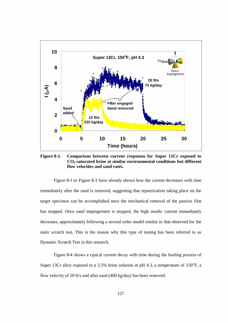
127
0
2
4
6
8
10
0 5 10 15 20 25 30Time (hours)
I( m
A)
Sandadded
Filter engagedSand removed
15 ft/s235 kg/day
20 ft/s75 kg/day
Super 13Cr, 150oF, pH 4.3Flow
ImpingementDirect
Figure 8-3. Comparison between current responses for Super 13Cr exposed toCO2-saturated brine at similar environmental conditions but differentflow velocities and sand rates.
Figure 8-1 to Figure 8-3 have already shown how the current decreases with time
immediately after the sand is removed, suggesting that repassivation taking place on the
target specimen can be accomplished once the mechanical removal of the passive film
has stopped. Once sand impingement is stopped, the high anodic current immediately
decreases, approximately following a second order model similar to that observed for the
static scratch test. This is the reason why this type of testing has been referred to as
Dynamic Scratch Test in this research.
Figure 8-4 shows a typical current decay with time during the healing process of
Super 13Cr alloy exposed to a 3.5% brine solution at pH 4.3, a temperature of 150oF, a
flow velocity of 20 ft/s and after sand (400 kg/day) has been removed.

128
0
5
10
15
20
25
30
0 0.5 1 1.5 2 2.5Time (hours)
I( m
A)
Super 13Cr
Temp: 150oF, pH 4.3Sand rate: 400 kg/dayVelocity: 20ft/s
Flow
ImpingementDirect
Figure 8-4. Anodic current decay for Super 13Cr alloy after sand is removedfrom the test cell loop.
How fast the current decays with time is determined by the healing rate of the
protective layer, and may depend on many variables such as temperature, pH, flow
velocity and material tested. Notice that the healing time frame is different from that
shown by the static scratch test for the same material at the same environmental
conditions (T and pH) showed in Chapter 5. For the scratch test of Super 13Cr at pH 4
and 150oF, after only 200 sec, the current has decreased to a value about 2% of the initial
current. On the other hand, for the dynamic flow loop test conducted at similar
environmental conditions and sand, the current has decreased to about 5% of the initial
current after 2 hours that sand was removed.

129
In any case, the current response for the flow loop test is also following a second
order model as shown in Figure 8-5. However, the parameters Io and m obtained for flow
loop tests typically show a significant difference to those observed for the static scratch
test at similar environmental conditions. Some possible explanations for this observation
are presented in Chapter 9.
1/ I = 229t + 26928
0.0E+00
5.0E+04
1.0E+05
1.5E+05
2.0E+05
2.5E+05
3.0E+05
0 200 400 600 800 1000 1200
Time (sec)
1/I
(1/A
) 1/ I = mt + 1/ I o
Super 13CrTemp: 150oFSand Added: 400 kg/dayVelocity: 20ft/s
Flow
ImpingementDirect
Figure 8-5. A linear behavior between 1/I and time after sand is removed fromthe test cell loop.
Figure 8-6 shows the anodic current decay data previously shown in Figure 8-4
along with the current vs. time obtained by using the second order model approximation.
This figure suggests that the second order model is in fact a very good approximation to
describe the repassivation process of CRAs under dynamic flow conditions tested for a
significant long period of time.

130
0
5
10
15
20
25
30
0 0.5 1 1.5 2 2.5
Time (hours)
I(mA
)
Actual Data2nd Order Model
Io = 28 mAm = 229 (1/A*s)
Super 13CrTemp: 150oFSand rate: 400 kg/dayVelocity: 20ft/s
Flow
ImpingementDirect
Figure 8-6. Actual data and second order model for the anodic current decayafter sand is removed from of the test cell loop.
Figure 8-7 shows the effect of sand rate on the anodic current decay of Super
13Cr at fixed environmental and flow conditions. This figure corroborates the trend
observed and discussed about Figure 8-2, i.e., for given environmental and flow
conditions, the higher the sand rate the higher the current (Io). Figure 8-7 also shows
similar behavior in the current vs. time response regardless of the sand rate. Figure 8-8,
shows how the sand rate only very slightly affects the value of the slope of the second
order model for the same data series seen in Figure 8-7.

131
0
5
10
15
20
25
30
0 1 2 3 4 5
Time (hours)
I( m
A)
400 Kg/day
200 Kg/day
75 Kg/day
Super 13CrT = 150oF, pH 4.3
Flow Velocity: 20 ft/s
Flow
ImpingementDirect
Figure 8-7. Effect of sand rate on the anodic current decay of Super 13Cr alloy.
1/ I = 204 t + 229,65675 Kg/day
1/ I = 198 t + 94,533200 Kg/day
1/ I = 229 t + 26,928400 Kg/day
0.E+00
1.E+05
2.E+05
3.E+05
4.E+05
5.E+05
0 200 400 600 800 1000
Time (sec)
1/I
(1/A
)
1/ I = mt + 1/ I o
Super 13Cr
T = 150oF, pH 4.3Flow Velocity: 20 ft/s
Figure 8-8. Effect of sand rate on the linear behavior for 1/I with time after sandis removed from the test cell loop.

132
Figure 8-9 shows the anodic current decay for 13Cr alloy after sand is removed
from the test cell loop. Initial currents are generally higher than those observed for Super
13Cr alloy at similar environmental and flow conditions. Also, the repassivation time
tends to be longer for 13Cr than for Super 13Cr at given conditions. These particular tests
were conducted at 150oF, sand rate of 60kg/day, at two different pH values of 4.3 and 6,
and two different flow velocities 20ft/s and 17ft/s, respectively. The current for both
conditions approximate the second order model.
0
5
10
15
20
25
30
35
40
0 0.5 1 1.5 2 2.5
Time (hours)
I( m
A)
13Cr
Temp: 150oF, pH 4.3 & 6Sand rate: 60 kg/day
20 ft/s, pH 4.3
17 ft/s, pH 6
Flow
ImpingementDirect
Figure 8-9. Effect of pH on the anodic current decay of 13Cr alloy.
The current magnitude for the test conducted at pH 4.3 is slightly higher than that
for the test conducted at pH 6, at least for the first hour. This difference in current
magnitude may correspond to the combined effect of the higher velocity and lower pH
and in any case it seems to be not too large. However, the time frames during which sand
133
flowed in the test cell loops for the two tests were significantly different, about 3 hours
for the test at pH 6, and just 5 minutes for the test at pH 4.3. If longer periods of time
were used to test 13Cr alloy at severe conditions such a low pH, high flow velocities and
high sand rates, high current magnitudes may be sustained, even after removing the sand,
thus not following the second order repassivation model.
When high currents are maintained for long periods of time in 13Cr, a black
coating grows on the surface of the 13Cr target specimen as seen in Figure 8-10a and
Figure 8-10b shows the metallic surface of 13Cr also exposed to severe environments
(low pH, high flow velocity and high sand rate) but just for a short period of time (about
5 minutes). Hence, the image shown in Figure 8-10b may be assumed to be a typical
initial stage of the black coating. The concentric ring pattern shown on the surface of the
13Cr specimen suggests that the erosion-corrosion damage is not uniform, being worse in
the dark zones. This pattern, matches material degradation patterns obtained with
computational fluid dynamics simulations performed for erosion and erosion-corrosion,
which are discussed in next chapter. If the combined mechanical and environmental
conditions are not that severe, for example, similar high flow velocities and sand rates but
higher pH, the black coating formation is prevented, the second order repassivation
behavior is followed and a typical CRA surface finish is obtained as shown in Figure 8-
10c. This observation also agrees with the common lower current values, corrosion rates
and erosion-corrosion rates obtained for 13Cr tested at pH 6 as compared to those
obtained for 13Cr tested at lower pH values. However, even at high pH values, the
resultant surface for 13Cr is still dull as compared to the bright mirror surface obtained
for super 13Cr at any pH. (see Figure 8-10d).
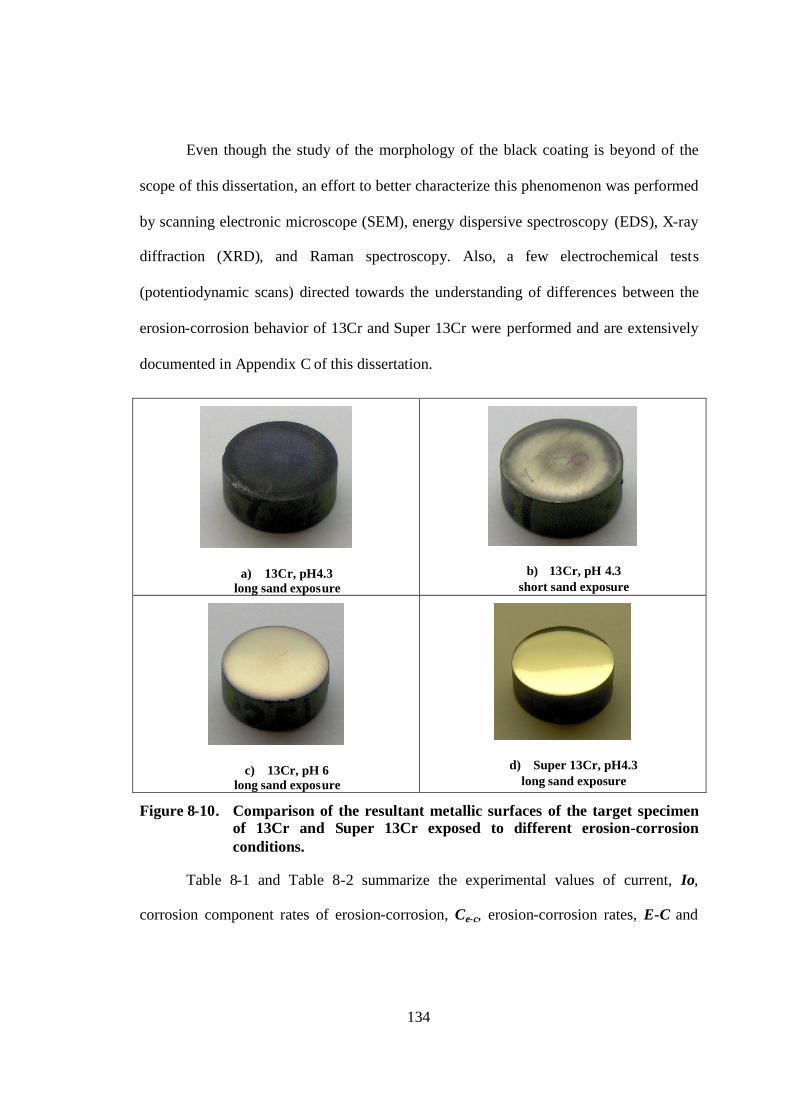
134
Even though the study of the morphology of the black coating is beyond of the
scope of this dissertation, an effort to better characterize this phenomenon was performed
by scanning electronic microscope (SEM), energy dispersive spectroscopy (EDS), X-ray
diffraction (XRD), and Raman spectroscopy. Also, a few electrochemical tests
(potentiodynamic scans) directed towards the understanding of differences between the
erosion-corrosion behavior of 13Cr and Super 13Cr were performed and are extensively
documented in Appendix C of this dissertation.
a) 13Cr, pH4.3long sand exposure
b) 13Cr, pH 4.3short sand exposure
c) 13Cr, pH 6long sand exposure
d) Super 13Cr, pH4.3long sand exposure
Figure 8-10. Comparison of the resultant metallic surfaces of the target specimenof 13Cr and Super 13Cr exposed to different erosion-corrosionconditions.
Table 8-1 and Table 8-2 summarize the experimental values of current, Io,
corrosion component rates of erosion-corrosion, Ce-c, erosion-corrosion rates, E-C and
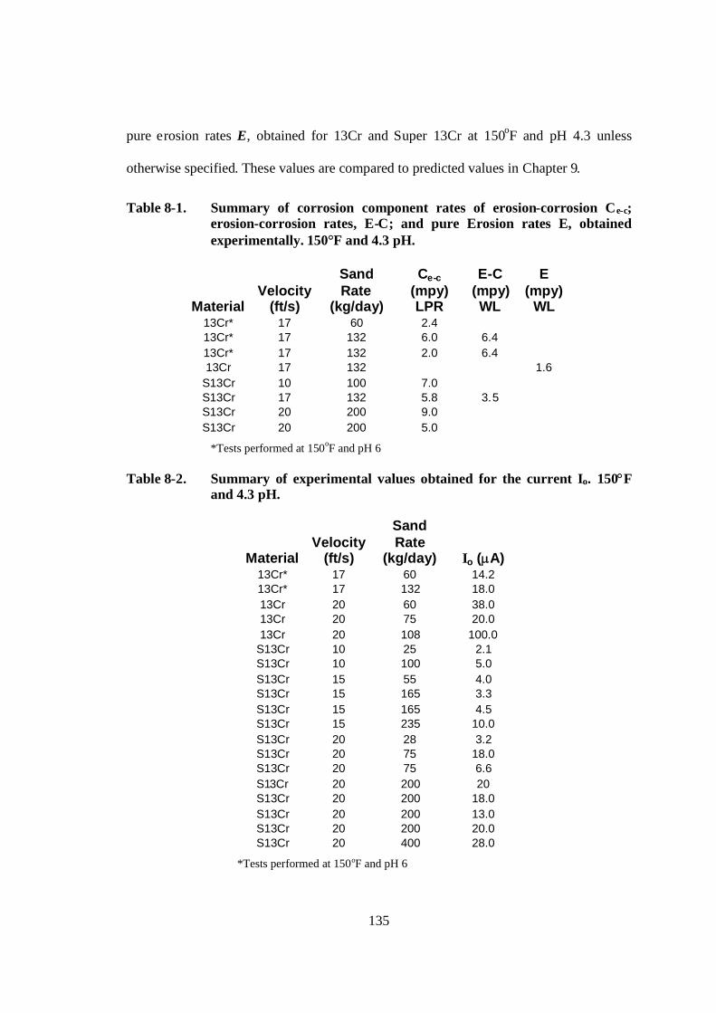
135
pure erosion rates E, obtained for 13Cr and Super 13Cr at 150oF and pH 4.3 unless
otherwise specified. These values are compared to predicted values in Chapter 9.
Table 8-1. Summary of corrosion component rates of erosion-corrosion Ce-c;erosion-corrosion rates, E-C; and pure Erosion rates E, obtainedexperimentally. 150F and 4.3 pH.
MaterialVelocity
(ft/s)
SandRate
(kg/day)
Ce-c
(mpy)LPR
E-C(mpy)WL
E(mpy)
WL13Cr* 17 60 2.413Cr* 17 132 6.0 6.413Cr* 17 132 2.0 6.413Cr 17 132 1.6
S13Cr 10 100 7.0S13Cr 17 132 5.8 3.5S13Cr 20 200 9.0S13Cr 20 200 5.0
*Tests performed at 150oF and pH 6
Table 8-2. Summary of experimental values obtained for the current Io. 150Fand 4.3 pH.
MaterialVelocity
(ft/s)
SandRate
(kg/day) Io (A)13Cr* 17 60 14.213Cr* 17 132 18.013Cr 20 60 38.013Cr 20 75 20.013Cr 20 108 100.0
S13Cr 10 25 2.1S13Cr 10 100 5.0S13Cr 15 55 4.0S13Cr 15 165 3.3S13Cr 15 165 4.5S13Cr 15 235 10.0S13Cr 20 28 3.2S13Cr 20 75 18.0S13Cr 20 75 6.6S13Cr 20 200 20S13Cr 20 200 18.0S13Cr 20 200 13.0S13Cr 20 200 20.0S13Cr 20 400 28.0
*Tests performed at 150oF and pH 6

136
CHAPTER 8 ..............................................................................................................................................122
SUBMERGED DIRECT IMPINGEMENT TEST: SINGLE PHASE LIQUID FLOW ................................ ..................122Erosion-Corrosion Liquid/Sand Loop (Microloop) ................................................................ ...........122
TABLE 8-1. SUMMARY OF CORROSION COMPONENT RATES OF EROSION-CORROSION CE-C; EROSION-CORROSION RATES, E-C; AND PURE EROSION RATES E, OBTAINED EXPERIMENTALLY. 150F AND 4.3PH. 135
TABLE 8-2. SUMMARY OF EXPERIMENTAL VALUES OBTAINED FOR THE CURRENT IO. 150F AND 4.3 PH.135
FIGURE 8-1. CURRENT RESPONSE FOR SUPER 13CR EXPOSED TO CO2 SATURATED BRINE CONTAININGSAND. 125
FIGURE 8-2. COMPARISON BETWEEN CURRENT RESPONSES FOR SUPER 13CR EXPOSED TO CO2-SATURATEDBRINE AT SIMILAR ENVIRONMENTAL AND FLOW CONDITIONS BUT DIFFERENT SAND RATES . ..............126
FIGURE 8-3. COMPARISON BETWEEN CURRENT RESPONSES FOR SUPER 13CR EXPOSED TO CO2-SATURATED
BRINE AT SIMILAR ENVIRONMENTAL CONDITIONS BUT DIFFERENT FLOW VELOCITIES AND SAND RATES.127
FIGURE 8-4. ANODIC CURRENT DECAY FOR SUPER 13CR ALLOY AFTER SAND IS REMOVED FROM THE TESTCELL LOOP. ................................................................................................................................ .........128
FIGURE 8-5. A LINEAR BEHAVIOR BETWEEN 1/I AND TIME AFTER SAND IS REMOVED FROM THE TEST CELL
LOOP. 129FIGURE 8-6. ACTUAL DATA AND 2ND ORDER MODEL FOR THE ANODIC CURRENT DECAY AFTER SAND IS
REMOVED FROM OF THE TEST CELL LOOP................................................................. ...........................130FIGURE 8-7. EFFECT OF SAND RATE ON THE ANODIC CURRENT DECAY OF SUPER13CR ALLOY................131FIGURE 8-8. EFFECT OF SAND RATE ON THE LINEAR BEHAVIOR FOR 1/I WITH TIME AFTER SAND IS REMOVED
FROM THE TEST CELL LOOP. ................................................................................................................131FIGURE 8-9. EFFECT OF PH ON THE ANODIC CURRENT DECAY OF 13CR ALLOY........................................132FIGURE 8-10. COMPARISON OF THE RESULTANT METALLIC SURFACES OF THE TARGET SPECIMEN OF 13CR
AND SUPER 13CR EXPOSED TO DIFFERENT EROSION-CORROSION CONDITIONS. ................................ ..134

136
CHAPTER 9
EROSION-CORROSION MODEL
The complexity of the chemi-mechanical mechanisms involved in erosion-
corrosion of CRAs under slurry flows has been mentioned on in previous chapters. The
many variables involved in the erosion-corrosion process such a temperature, pH, flow
velocity, sand rate, and material type have been described and discussed. How these
parameters affect the erosion-corrosion mechanism was carefully studied by means of
different experimental techniques during this research period. Some of these parameters
may need further study and many other parameters such water chemistry, chloride
contents, H2S, and material properties may be included in future research work. However,
there is an immediate need to define safe service limits for utilization of such materials in
a great diversity of corrosive oil and gas environments which contain sand particles. As
an initial effort to address this need a framework for an erosion-corrosion prediction
model is presented in this Chapter.
General Approach
The concept of a synergistic effect between chemical and mechanical processes
found in erosion-corrosion conditions was introduced in previous chapters. Even though
no uniform nomenclature has been used to define the terms contributing to the total

137
erosion-corrosion weight loss, many authors agree on the need to consider four terms.64-68
The first two terms usually account for the chemical degradation and the mechanical
degradation as separate processes, and here they are named as pure corrosion, C and pure
erosion, E. The two remaining terms describe the synergism involved in the erosion-
corrosion process; one accounts for the corrosion increment due to erosion, Ce and the
other accounts for the erosion increment due to corrosion, Ec. Hence, the total erosion-
corrosion rate EC is given by equation 9-1.
ce ECECEC (9-1)
Determining whether there is a dominant term is not straight forward, and often
depends on the combined effect of environmental and mechanical variables as well as
material properties. However, existing erosion-corrosion data have provided enough
understanding of the process to make reasonable assumptions in regards to simplifying
the procedures to predict erosion-corrosion under specific conditions.
A mechanistic procedure to estimate erosion-corrosion penetration rates for CRAs
exposed to CO2 saturated brine/sand flows conditions was constructed and is described in
the following paragraphs. The procedure is based on experimental data obtained from
static scratch tests and on computation fluid dynamics (CFD) simulations. Experimental
and numerical data are integrated into the model and processed with a VBA code to
numerically estimate the erosion-corrosion penetration rate. The model assumes some
fixed parameters such a brine concentration, water chemistry, and CO2 pressure. Input
parameters are temperature, pH (which are implicit in the second order scratch test
parameters, m and Io), type of alloy, sand rate, sand size, and liquid velocity.
138
Output of the model includes the pure erosion rate, E, the total erosion-corrosion
penetration rate, EC, and the corrosion rate component of the erosion-corrosion process,
Ce-c, defined as the sum of the pure corrosion C and the impact-induced corrosion Ce
expressed as follow
ece CCC (9-2)
The Ce-c component conveniently groups those terms describing chemical
degradation since they are experimentally measured together when electrochemical
techniques are used to estimate penetration rates for flows containing solid particles.
Hence, direct comparisons between the model and experimental data can be made. For
the purpose of this research, an additional output was considered as the total current, Io,
to be compared with experimental data shown in Chapter 8.
Results of a previous investigation57,59 performed for erosion-corrosion of 13Cr
alloy exposed to CO2 saturated brine/sand flows, suggested that the total erosion-
corrosion penetration rate for this environment and alloy combination equals the sum of
the pure erosion term E, and the corrosion component of the erosion-corrosion term Ce-c.
This means that the corrosion-induced erosion term, Ec, was negligible for these tested
conditions. Based on this finding, the model estimates the total erosion-corrosion
neglecting the term Ec, as follow.
ceCEEC (9-3)

139
The pure erosion term, E, is estimated from the computational fluid dynamics
procedure explained in Appendix D, and Ce-c is estimated with a new procedure
developed in this research.
Proposed Procedure for Estimating Ce-c.
The estimation of the corrosion component of erosion-corrosion, Ce-c, has its
foundation on a model that reasonably describes the competition between the mechanical
removal of the passive film due to solid particle impingement and the re-formation of this
protective film due to the electrochemical repassivation process. The mechanical part of
the model relies on the particle tracking and erosion modeling executed with CFD, while
the electrochemical process relies on the second order model displayed by the
experimental data obtained with the scratch test technique. The physical model to explain
the higher currents observed when sand is introduced into the flow as compared with the
low passive currents typically observed for CRAs exposed to sand-free brine flows, is
shown schematically in Figure 9-1.

140
rR
Base Metal
tT
X
X
IndentationPassive film
Particle
Removed material
rR
Base Metal
tT
X
X
IndentationPassive film
Particle
Removed material
Figure 9-1. Schematic of a particle impingement on a passive alloy.
Figure 9-1 shows an ideal spherical particle of radius R that has impacted a
passive material. The impact resulted in a spherical indentation in the metallic surface
which is shown with a maximum penetration depth x. Also the volume of material
(passive layer and base metal) displaced by the impact is shown in the same figure
forming a platelet shape, as described in an erosion model proposed by Finnie50.
The similarity between the scratch test and the erosion-corrosion process for a
single solid particle impact was discussed in Chapter 5. At given environmental
conditions (pH and temperature), the amount of current or corrosion taking place in the
scratch test can be assumed to be the same as that due to a single solid particle impact
provided that the scratched area and the indented area are identical. In other words, the
increment in current due to removal of the passive layer does not depend on how the
141
passive layer was removed (scratch or particle impact) but on how much exposed (bare,
without passive layer) area was created. Hence, the current density is assumed to be the
same for both processes provided that environmental conditions were the same.
If the current density is known, determination of the amount of the open (bare)
area of the base metal created (due mechanical film removal) by a particle impact is the
only additional quantity needed to estimate the increment in corrosion due to that particle
impact. Then, the remaining key parameters to be considered in the erosion-corrosion rate
determination are the time frame that the open (bare) surface will take to re-form the
passive film after each particle strike, and the particle impact frequency.
At this point the healing rate represented by the slope m of the second order
model figures into the prediction model. The initial current density is given by the scratch
test, and the open area is determined using the solid particle information from the CFD
erosion model. The slope of the second order model describes the rate of decay of the
initial current density for each particle impact. Therefore, if the number of particles that
hit a particular cell is known (computed from the CFD simulation) the total current
generated per cell can be computed. Also, the current for the whole target specimen can
be estimated by adding the currents from each cell, allowing for computation of the total
corrosion component of the erosion-corrosion process.
142
Determination of the indented open area
The determination of the indented surface area created in the base metal is not too
different from the estimation of the volume of material removed due to the particle
impingement. Ultimately, both the indented area and the volume of material removed are
caused by the same impingement. Thus, one can reasonably assume that the variables
affecting the variation of the indented area are similar to those affecting the material
removal and erosion rates.
Furthermore, if the volume of material removed is assumed to be equal to the
volume of the indented space, the volumetric erosion ratio is then equal to the ratio of the
volume of the indented area to the volume of the spherical particle causing the
indentation given by
volumeimpactingsand
materialremoved
sphere
nindentatio ERV
V
VV
_
_ (9-4)
where the volumetric erosion ratio is the mass erosion ratio (kg of removed material/kg of
sand impacting) multiplied by the inverse of the ratio of the density of the target material
and the erodent particle, given by.
material
particlemassvolume ERER
(9-5)
Also a relation between the ratio of the volume of the indentation to the volume of
a sphere and the ratio of the surface area of the indentation to the surface area of a sphere
was found to be closely approximated by equation (9-6). (See details in Appendix E)

143
5026.0
6022.0
sphere
nindentatio
sphere
nindentatio
VV
SS (9-6)
If equations (9-4) and (9-5) are substitute into equation (9-6), the surface of the
indentation caused by a single impact can be computed as a function of the erosion ratio,
the densities of the target material and erodent particle, and the particle size as shown in
equation (9.7)
25026.0
6022.0 pmaterial
particlemassnindentatio DERS
(9-7)
where Dp is the diameter of the particle.
Since the function obtained for determination of the area of the indentation
strongly depends in the erosion ratio, the indented area is expected to vary with impact
velocity and impact angle in a similar fashion as the erosion ratio does. Furthermore, the
same material removal mechanisms considered in the erosion equation by Oka et.al.61,
namely “cutting action” and “repeated plastic deformation” are also being considered in
the estimation of the indented area and therefore in the corrosion component of the
erosion-corrosion process.
Implementation of the second order model to determine the total current
Using equation (9-7) the area of the indentation where the passive layer has been
removed by the particle impact can be estimated. With the current density obtained from
the scratch tests and the known surface area of the indentation, the initial current, Io,
generated for each particle impact can be estimated. Notice, each particular impingement

144
will have its own impact characteristics (impact speed and impact angle) causing a
specific erosion ratio and thus a particular indentation area. Therefore, each impact will
generate a different amount of current.
From the CFD simulation, the impact frequency (# particles per second) for each
cell is also known and can be used to estimate the time between impacts, tbp for that
specific cell as the inverse of the impact frequency. With the estimated current, Io,
produced by the particle impact, the slope, m, from the scratch test and the time between
particles, tbp, the total current generated by all the particle impacts taking place in a
particular cell as a function of time can be estimated. To achieve this, the second order
model is used to compute the current transients caused by each particle impact. The total
current per cell is then estimated by adding the current transients due to each particle
impact which are a time, tbp, apart from each other as seen in Figure 9-2.
The continued addition of the high initial current values as additional sand
particles strike causes a repeating behavior of the total current series. Still, the total
current trend seems to increase with time and tends to stabilized for large times when the
tails of the first impingements are negligible as compared with the value of total current
for the same time. Thus, a range of current, more than a single value is expected when the
stabilized current is reached after some time has past, as depicted by Figure 9-3.

145
0
1
2
3
4
5
6
7
8
9
0.0 0.3 0.5 0.8 1.0 1.3 1.5 1.8 2.0 2.3 2.5 2.8 3.0Time
I( m
A)
1st Imp.2nd Imp.3rd Imp.
4th Imp.5th Imp.6th Imp.Itotal
t bp
Total currentgenerated in acell impactedby 6 particles
t total
Figure 9-2. Generic plot for the total current and individual current transients of
6 different impacts taking place in a numerical cell of the target
specimen.
Figure 9-3 only shows the total current also shown in Figure 9-2 but, now
includes the trends observed for the peaks, and valleys displayed by the cyclic total
current series. If only the values of the peaks and valleys are estimated and averaged a
average trend with a single value for the total Io current can be estimated.
Notice that the size of the range between the peaks and the valleys of the total
current would decrease by decreasing the time between particles, tbp. In fact, the typical
impact frequencies obtained for the simulated conditions considered in this study were
high (hundreds of particles per second), therefore, values of tbp are so small that trend
curves for the peaks and valleys and the average trend lie on top of each other.

146
0
1
2
3
4
5
6
7
8
9
0.0 0.3 0.5 0.8 1.0 1.3 1.5 1.8 2.0 2.3 2.5 2.8 3.0Time
I( m
A)
Itotal
t bp
peaks trend
valleys trend
Avg trendtotal I o
Figure 9-3. Generic plot for the total current generated in a cell due to total
particle impact.
Notice also that for the prediction, the total current will not ever completely
stabilize since the tails of the transients will never reach absolute zero (see Figure 9-2).
Therefore, a stop criterion is needed to determine an appropriate value for ttotal. An
intuitive value for the total time is not easy to determine other than one that is large
enough to yield an acceptably accurate result. For this reason, the stop criterion was
designed in a way that the value will emerge from the same simulation. Hence, the
numerical summation of the transient currents stops when the current added for the last
particle impact causes an increment equal or less of 1/10,000th of the total current
summed up to the previous time step. The criterion seems to work reasonably well and
Figure 9-4 shows the total cell current for a cell with an impact frequency of 74 particles
per second. The continuous curve representing the total current has significantly bent
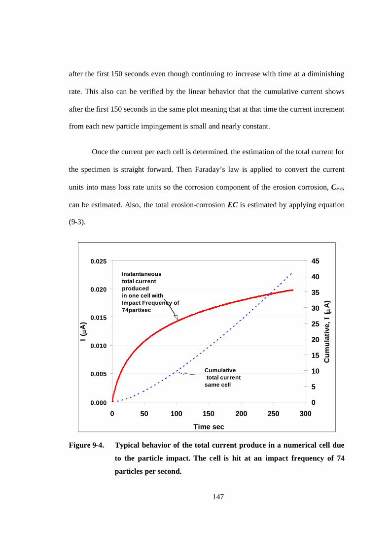
147
after the first 150 seconds even though continuing to increase with time at a diminishing
rate. This also can be verified by the linear behavior that the cumulative current shows
after the first 150 seconds in the same plot meaning that at that time the current increment
from each new particle impingement is small and nearly constant.
Once the current per each cell is determined, the estimation of the total current for
the specimen is straight forward. Then Faraday’s law is applied to convert the current
units into mass loss rate units so the corrosion component of the erosion corrosion, Ce-c,
can be estimated. Also, the total erosion-corrosion EC is estimated by applying equation
(9-3).
0.000
0.005
0.010
0.015
0.020
0.025
0 50 100 150 200 250 300
Time sec
I( m
A)
0
5
10
15
20
25
30
35
40
45
Cu
mu
lati
ve,I
( mA
)
Instantaneoustotal currentproducedin one cell withImpact Frequency of74part/sec
Cumulativetotal current
same cell
Figure 9-4. Typical behavior of the total current produce in a numerical cell due
to the particle impact. The cell is hit at an impact frequency of 74
particles per second.

148
Figure 9-5 shows the flow chart for the complete prediction procedure of erosion-
corrosion of CRAs in brine flows containing sand. It includes the experimental scratch
test work, the CFD modeling, the mechanistic approach of the chemi-mechanical
degradation process, the erosion loop testing needed to adjust the CFD predicted erosion
rates, the erosion-corrosion loop testing to compare the predicted values for the corrosion
component of the erosion-corrosion Ce-c, and the total erosion-corrosion, EC.

149
Particle Io
Add Individual Particle Current&
Estimate Total Cell Current
Scratch TestOutput,
m, io
AdjustedErosion
IndentationArea
CFD Output,Impact frequency, impact
velocity, impact angle, impactlocation.
Scratch Test,Vary, temp, pH and
Material
Estimate Total Specimen Current&
Faraday law Ce-cEstimate
EC
ErosionWL
Loop Testing
CFD Input,Flow velocity, sand rate
flow geometry
LPR and WLLoop Testing to
compare Ce-c & EC
Figure 9-5. Flow diagram to estimate E, Ce-c, & EC

150
Validation of the Erosion-Corrosion Prediction Model
The procedure to estimate the penetration rates (E, Ce-c and EC) shown in Figure
9-5, was built into a computational code (VBA) to be able to generate prediction results
and compare them to gathered experimental data. A series of prediction cases was run for
a broad range of flow velocity, sand rate, temperature, and pH values. Cases include
predictions for 13Cr, Super 13Cr and 22Cr alloys.
Adjustment of the erosion prediction
Before comparisons between predicted values and experimental results were
done, an adjustment of the erosion model was needed. Appendix D describes the over-
prediction of erosion rates for all cases run following the state-of-the-art in CFD
simulation. A factor F, with a value of 125 units, was used in the denominator of the
erosion equation proposed by Oka and Yoshida62 shown as equation (D-7) in Appendix
D.
The F factor was determined by matching the predicted erosion rate to
experimental flow loop data for pure erosion (obtained by weight loss) shown in Chapter
8. Difficulties obtaining reliable experimental data in erosion by liquid-sand flows were
discussed in Chapter 8. Hence, F=125 should not considered to be a precise number and,
a new adjustment based in more reliable experimental data is recommended for future
purposes. In any case, the present adjustment, allows the prediction of erosion rates to be
within the right order of magnitude.

151
Comparison between experimental data and predictions
Figure 9-6 shows the comparison between the measured erosion and erosion-
corrosion rates obtained by weight loss with those predicted by the proposed model. Only
the pure erosion data point shown in this figure was adjusted. From the two erosion-
corrosion data points included in the plot, it can be seen one of them in perfect agreement
with the prediction while the remaining data point seems to be a little over predicted by
the model. However, considering that no further adjustments or any fitting constants were
used for the estimates of the corrosion component of erosion-corrosion and the total
erosion-corrosion rates, Figure 9-6 suggests reasonably good agreement between
measured and predicted values. And again, it should be noted that all the experimental
data represented in Figure 9-6 was gathered for experimental conditions yielding quite
low weight losses for which significant error is possible.
0
1
2
3
4
5
6
7
0 1 2 3 4 5 6 7
E or EC Experimental
E,o
rE
CM
od
el
ECE
S13Cr, pH=4
13Cr, pH=6
Flow
ImpingementDirect
Figure 9-6. Comparison between measured erosion and erosion-corrosion
penetration rates (by weight loss) and those predicted by the proposed
model.
152
Figure 9-7 shows the comparison between the measured corrosion component
rates Ce-c by linear polarization resistance (LPR) and those predicted by the proposed
model. A reasonable agreement between experimental data and predicted results can be
seen if the experimental data point at 7 mpy is ignored even though some scatter still
exists around the perfect agreement line. However, some scatter of the experimental data
is a fact of life when LPR data is collected. Studies 63 performed to check reproducibility
of the LPR technique have suggested error factors of up to 2 in corrosion rates measured
when using this technique without Tafel slope adjustment. In addition, the LPR values
(and the scale shown for this figure) are small when compared to the scale often
associated with erosion, corrosion and erosion-corrosion data showing much higher mpy
values, generally found at higher flow velocity conditions. Recently a new higher
velocity single phase liquid flow loop capable of handling CO2-saturated brines and sand
has been constructed. Experimental data collected for liquids-sand flows at higher
velocities of 20-40 ft/s would provide more reliable experimental data and perhaps a
better test for the present erosion-corrosion prediction model.
Figure 9-8 shows the comparison between the total current values (A) as
measured with the scratch test instrumentation adapted to the flow system and those
values predicted by the proposed model. Again, some scatter is shown but a good trend is
observed for the model predictions in comparison with experimental data. These
predictions are encouraging considering that no adjustments or fitting constants at all
were used for the corrosion component of the predictive model and the single adjustment
made for the erosion component of the model was based on only one set of experimental
conditions.

153
0
1
2
3
4
5
6
7
8
9
10
0 1 2 3 4 5 6 7 8 9 10
C e-c (mpy) Experimental (LPR)
Ce-
c(m
py)
Mo
del
Flow
ImpingementDirect
Figure 9-7. Comparison between measured corrosion component penetration
rates (by LPR) and those predicted by the proposed model.
0
5
10
15
20
25
30
35
40
45
0 5 10 15 20 25 30 35 40 45I (mA) Experimental
I(
A)
Mod
el
Flow
ImpingementDirect
Figure 9-8. Comparison between measured total current values (A) and those
predicted by the proposed model.

154
Another point to consider when evaluating these comparisons is related to the
number of variables that the model is taking into account to predict erosion-corrosion.
The proposed model considers temperature, pH, flow velocity, sand rate, sand properties,
flow geometry and material type. From this point of view, experimental data and
predicted values may consider to be in reasonably good agreement.
Some trends of predicted values
The following sections of this chapter display the trends of predicted values when
varying some of the variables such as temperature, pH, sand rate, flow velocity and
material type. The experimental data shown in previous plots are inserted into figures
showing trends. In addition, a new set of comparisons between the predictions and other
sets of experimental data discussed in Chapter 2 and Chapter 7 are included.
Effect of sand rate: comparison between experiments and prediction trends
Figure 9-9 shows trends for predicted pure erosion rates with sand rates for
different flow velocities. Trends with sand rates and velocities are as expected, that is,
increasing erosion rate for increasing sand rate and increasing flow velocity. A type of
saturation effect for the erosion rate in direct impingement experiments is usually
observed at high sand rates due to shielding. This phenomenon consists of a blockage
provided by a front of sand particles, which bouncing back from the target, form a shield
in front of it providing some protection from new impingements from trailing particles.
CFD simulations do not take this effect into account so the predicted erosion rates are
linearly increasing with the sand rate regardless of how high is the sand concentration.
Erosion rates seen in Figure 9-9 were obtained for CFD simulations performed for 13Cr,

155
the trends for Super 13Cr are exactly the same, but the values are slightly lower. This
variation is due to the differences in hardness of the two alloys being 25Rc for 13Cr and
30Rc for Super 13Cr. The effect of hardness in erosion has been a controversial topic;
some trends of erosion rates with hardness have been found provided that the
microstructure of the alloys compared are similar. Even so, the effect of material
hardness on erosion rate is only a small one in comparison with the effect of other
parameters such as flow velocity, erodent concentration and erodent properties.
0
1
2
3
4
5
6
7
0 100 200 300 400
Sand Rate (kg/d)
Pen
etra
tio
nR
ate
(mp
y)
E 10ftsE 15ftsE 17fts
E 20fts
TargetSpecimen
Flow
Jet
Figure 9-9. Prediction trends with sand rate of pure erosion, E for several flow
velocities.
Figure 9-10 shows the prediction trends with sand rate of pure erosion, E and
corrosion component of erosion-corrosion, Ce-c for Super 13Cr at two flow velocities.
Predicted trends with sand and velocity are as expected: the erosion rate and the corrosion

156
component of erosion-corrosion increase with both flow velocity and sand rate. Also, the
corrosion component of erosion corrosion rates are higher than the pure erosion rates as
have been seen for experiments with Super 13Cr conducted at relatively low erosivity
conditions presented in Chapter 7. Figure 9-10 also includes 3 experimental data points.
Predictions slightly underestimate the experimental values at both velocities, but
considerable scatter is also shown for experiments conducted at 20ft/s, whose average of
6.5 mpy, accurately matches the predicted value.
0
2
4
6
8
10
12
0 100 200 300 400 500Sand Rate (kg/d)
Pen
etra
tio
nR
ate
(mp
y)
E 20fts
E 17fts
Ce-c 20fts
Ce-c 17fts
Ce-c 20fts (LPR)
Ce-c 17fts (LPR)
Super 13Cr, 150F, pH 4
TargetSpecimen
Flow
Jet
Figure 9-10. Prediction trends with sand rate of pure erosion, E and corrosion
component of erosion-corrosion, Ce-c for Super 13Cr at two flow
velocities.
Figure 9-11 shows a comparison for the same conditions but different material. It
shows the prediction trends with sand rate of pure erosion, E and corrosion component of

157
erosion-corrosion, Ce-c for 13Cr and Super 13Cr at 20ft/s and similar environmental
conditions (pH and 150oF). As expected, and seen in trends for experimental data shown
in Chapter 7, the corrosion component rates of 13Cr are significant higher than those for
Super 13Cr. Also notice how the estimated pure erosion rates for 13Cr and Super 13Cr
are fairly similar.
0
5
10
15
20
25
0 100 200 300 400 500
Sand Rate (kg/d)
Pen
etra
tio
nR
ate
(mp
y)
Ce-c, 13Cr
E, 13Cr
Ce-c, S13Cr
Ce-c, S13Cr (LPR)
E, S13Cr
150oF, pH 4
13Cr, C e-c
Super 13Cr, Ce-c
Erosion, 13Cr & Super 13Cr
TargetSpecimen
Flow
Jet
Figure 9-11. Comparison between 13Cr and Super 13Cr prediction trends with
sand rate of pure erosion, E and corrosion component of erosion-
corrosion, Ce-c.
Figure 9-12 shows a comparison for the same material exposed to different
environmental conditions. It shows the prediction trends of pure erosion, E and corrosion
component of erosion-corrosion, Ce-c for 13Cr at 20ft/s with increasing sand rate and
three different environmental conditions, pH4 at 150oF, pH4 at 200oF and pH6 at 150oF.

158
The corrosion component rates are in general higher than the pure erosion rates; but there
are significant differences among them. The highest corrosion component rates are
predicted for the combination of highest temperature, 200oF and the lowest pH value of 4.
If the pH is fixed at 4 and the temperature is decreased to 150oF, the corrosion component
rates decreases by about 40% (reduction % varies slightly with sand rate). If then, at a
fixed temperature of 150oF, the pH is increased up to 6, the corrosion component rates
further reduce an additional 30%. These trends are in agreement with experimental data
shown in Chapter 7. Figure 9-12 also includes a couple of experimental data point
obtained by using LPR technique for 13Cr exposed to pH 6 and 150oF. For these
conditions, the experimental data and the predicted corrosion component rates are in very
good agreement.
0
5
10
15
20
25
30
35
40
0 100 200 300 400 500
Sand Rate (kg/d)
Pen
etra
tion
Rat
e(m
py)
Ce-c, pH4, T=150 F
Ce-c, pH4, T=200F
Ce-c, pH6, T=150
Ce-c, pH6 T= 150 F, Exp
E
13Cr, 20 ft/s
pH 4, 200 o F, Ce-c
pH 4, 150 o F, Ce-c
pH 6, 150 oF, C e-c
pure Erosion
TargetSpecimen
Flow
Jet
Figure 9-12. Effect of pH and temperature on the prediction trends with sand rate
of the corrosion component of erosion-corrosion, Ce-c for 13Cr.

159
Effect of temperature: comparison between experiments and prediction trends
Unfortunately, most of the data shown in chapter 7 for erosion-corrosion testing
of CRAs were conducted at multiphase flow conditions (gas-liquid-sand) for plugged tee
geometry, while the CFD simulations were conducted for direct impingement in liquid-
sand flows. However the multiphase flow experimental data may be used to check the
trends with temperature and material given by the proposed model. Differences in the
magnitudes of the erosion-corrosion rates for multiphase flow conditions and single
phase liquid conditions are often large. Therefore to be able to compare them, all values
presented will be normalized to the erosion-corrosion value at 76oF.
Figure 9-13 shows the comparison between experimental data and predicted
values for 13Cr exposed to the same environmental conditions (pH and temperature) but
different flow conditions. Erosion-corrosion experimental data was conducted for
multiphase flow conditions (gas-liquid-sand) and plugged tee geometry while predicted
values were obtained for liquid sand flows for direct impingement. It is encouraging to
see in Figure 9-13 that, in spite of the huge differences in flow conditions, the proposed
model still is able to match the trends observed with temperature when the normalized
values are compared. Both model and experimental data suggest that erosion-corrosion
damage at 150oF is about 1.7 larger than that obtained at 76oF. Very good agreement
between experimental data and predicted trends with temperature were also obtained for
the other two alloys under study (Super 13Cr and 22Cr), as displayed in Figure 9-14 and
Figure 9-15. These results suggest that erosion-corrosion damage at 150oF for Super 13Cr
is about 1.4 times that obtained at 76oF, while for 22Cr, the erosion-corrosion damage at
150oF is only about 1.1 times that obtained at 76oF.

160
Effect of material: comparison between experiments and prediction trends
To be able to compare all these experimental data and predicted values shown for
the three CRAs on a single plot, all experimental values were normalized to the
experimental value of the erosion-corrosion rate of 13Cr at 76oF, and all predicted values
were normalized to the predicted value for erosion corrosion of 13Cr at 76oF.
0.0
0.2
0.4
0.6
0.8
1.0
1.2
1.4
1.6
1.8
0 20 40 60 80 100 120 140 160
Temperature (oF)
Eros
ion-
Co
rro
sio
n,E
C(m
py)
Model, Vl=15fts, 235kgd, Direct Impingement
Exp, Vsg=20fts, Vsl=1.4fts, 14.6kgd, Plugged T
13Cr, pH 4
Figure 9-13. Comparison between experimental data and predicted trends with
temperature of the erosion-corrosion of 13Cr. All data normalized to
room temperature values.

161
0.0
0.2
0.4
0.6
0.8
1.0
1.2
1.4
1.6
0 20 40 60 80 100 120 140 160
Temperature (oF)
Ero
sio
n-C
orr
osio
n,E
C(m
py)
Model, Vl=15fts, 235kgd, Direct Impingement
Exp, Vsg=20fts, Vsl=1.4fts, 14.6kgd, Plugged T
Super 13Cr, pH 4
Figure 9-14. Comparison between experimental data and predicted trends with
temperature of the erosion-corrosion of Super 13Cr. All data
normalized to room temperature values.
0.0
0.2
0.4
0.6
0.8
1.0
1.2
0 20 40 60 80 100 120 140 160
Temperature (o F)
Ero
sio
n-C
orro
sio
n,E
C(m
py)
Model, Vl=15fts, 235kgd, Direct Impingement
Exp, Vsg=20fts, Vsl=1.4fts, 14.6kgd, Plugged T
22Cr, pH 4
Figure 9-15. Comparison between experimental data and predicted trends with
temperature of the erosion-corrosion of 22Cr. All data normalized to
room temperature values.

162
Figure 9-16 shows the comparison between experimental data and predicted
values for the three CRAs as shown in Figure 9-13 to Figure 9-15, but collected in on
single plot. It is clearly seen how the model was able to completely grasp the trends for
the erosion-corrosion behavior of the three alloys with respect to CRA type and
temperature. These results are encouraging, especially when considering the complexity
of the phenomena under study and the large number of variables taken into account in the
model. It is recognized that there are some opportunities to improve the model and some
of the ideas for this are presented in Chapter 10.
0.00.20.40.60.81.01.21.41.61.8
No
rmal
ized
Ero
sion
Co
rro
sion
,EC
(ref
13C
r,76
F)
13CrExper.
13CrModel
S13CrExper.
S13CrModel
22CrExper.
22CrModel
76 150Temp.
oF
76150
Exp, Vsg=20ft/s, Vsl=1.4ft/s, 14.6 kg/d sand, Plugeed TeeModel, Vl=15ft/s, 235 kg/d sand, Direct Impingement
Figure 9-16. Comparison between experimental data and predicted trends of the
erosion-corrosion, EC of the three CRAs at two different
temperatures. All data normalized to 13Cr at room temperature
value.

163
CHAPTER 9 ................................................................................................................................136
EROSION-CORROSION MODEL ................................ ................................................................ ....136
General Approach ................................ ................................................................ ...............136
Proposed procedure for estimating Ce-c. ................................................................ .............139
Determination of the indented open area............................................................................................142
Implementation of the second order model to determine the total current.......................................143
Validation of the Erosion-Corrosion prediction model .......................................................150
Adjustment of the erosion prediction..................................................................................................150
Comparison between experimental data and predictions...................................................................151
Some trends of predicted values..........................................................................................................154
Effect of sand rate: comparison between experiments and prediction trends ..................................154
Effect of temperature: comparison between experiments and prediction trends .............................159
Effect of material: comparison between experiments and prediction trends....................................160
FIGURE 9-1. SCHEMATIC OF A PARTICLE IMPINGEMENT ON A PASSIVE ALLOY. ........................................140
FIGURE 9-2. GENERIC PLOT FOR THE TOTAL CURRENT AND INDIVIDUAL CURRENT TRANSIENTS OF 6
DIFFERENT IMPACTS TAKING PLACE IN A NUMERICAL CELL OF THE TARGET SPECIMEN. .....................145
FIGURE 9-3. GENERIC PLOT FOR THE TOTAL CURRENT GENERATED IN A CELL DUE TO TOTAL PARTICLE
IMPACT. 146
FIGURE 9-4. TYPICAL BEHAVIOR OF THE TOTAL CURRENT PRODUCE IN A NUMERICAL CELL DUE TO THE
PARTICLE IMPACT. THE CELL IS HIT AT AN IMPACT FREQUENCY OF 74 PARTICLES PER SECOND. .........147
FIGURE 9-5. FLOW DIAGRAM TO ESTIMATE E, CE-C, & EC ................................ .............................149
FIGURE 9-6. COMPARISON BETWEEN MEASURED EROSION AND EROSION -CORROSION PENETRATION RATES
(BY WEIGHT LOSS) AND THOSE PREDICTED BY THE PROPOSED MODEL................................. ...............151
FIGURE 9-7. COMPARISON BETWEEN MEASURED CORROSION COMPONENT PENETRATION RATES (BY LPR)
AND THOSE PREDICTED BY THE PROPOSED MODEL................................................................. .............153
FIGURE 9-8. COMPARISON BETWEEN MEASURED TOTAL CURRENT VALUES (A) AND THOSE PREDICTED BY
THE PROPOSED MODEL. .......................................................................................................................153
FIGURE 9-9. PREDICTION TRENDS WITH SAND RATE OF PURE EROSION, E FOR SEVERAL FLOW VELOCITIES.
155
FIGURE 9-10. PREDICTION TRENDS WITH SAND RATE OF PURE EROSION, E AND CORROSION COMPONENT
OF EROSION-CORROSION, CE-C FOR SUPER 13CR AT TWO FLOW VELOCITIES. ................................ ....156
FIGURE 9-11. COMPARISON BETWEEN 13CR AND SUPER 13CR PREDICTION TRENDS WITH SAND RATE OF
PURE EROSION, E AND CORROSION COMPONENT OF EROSION-CORROSION, CE-C. ...............................157
164
FIGURE 9-12. EFFECT OF PH AND TEMPERATURE ON THE PREDICTION TRENDS WITH SAND RATE OF THE
CORROSION COMPONENT OF EROSION-CORROSION, CE-C FOR 13CR................................. ..................158
FIGURE 9-13. COMPARISON BETWEEN EXPERIMENTAL DATA AND PREDICTED TRENDS WITH
TEMPERATURE OF THE EROSION-CORROSION OF 13CR. ALL DATA NORMALIZED TO ROOM
TEMPERATURE VALUES................................. ................................................................ ......................160
FIGURE 9-14. COMPARISON BETWEEN EXPERIMENTAL DATA AND PREDICTED TRENDS WITH
TEMPERATURE OF THE EROSION-CORROSION OF SUPER 13CR. ALL DATA NORMALIZED TO ROOM
TEMPERATURE VALUES................................. ................................................................ ......................161
FIGURE 9-15. COMPARISON BETWEEN EXPERIMENTAL DATA AND PREDICTED TRENDS WITH
TEMPERATURE OF THE EROSION-CORROSION OF 22CR. ALL DATA NORMALIZED TO ROOM
TEMPERATURE VALUES................................. ................................................................ ......................161
FIGURE 9-16. COMPARISON BETWEEN EXPERIMENTAL DATA AND PREDICTED TRENDS OF THE EROSION-
CORROSION, EC OF THE THREE CRAS AT TWO DIFFERENT TEMPERATURES. ALL DATA NORMALIZED TO
13CR AT ROOM TEMPERATURE VALUE................................................................. ...............................162
1 Rincon, H.E., Chen, J. and Shadley, J.R. (2002). Erosion-Corrosion Phenomena of
13Cr Alloy in Flows Containing Sand Particles. Corrosion/2002, paper no. 2493,
(Houston, TX, USA, NACE International.
2 Levy, A. “Mechanisms of Erosion” in Solid Particle Erosion and Erosion-Corrosion
of Materials, ASM International, Chapter 2, pp 11-25, 1995
3 Oka, Y.I, Okamura, K., Yoshida, T., “Practical estimation of erosion damage caused
by solid particle impact. Part 1: Effects of impact parameters on a predictive
equation.” Wear 259 (95-101)

165
4 Oka, Y.I, Yoshida, T., “Practical estimation of erosion damage caused by solid
particle impact. Part 2: Mechanical properties of materials directly associated with
erosion damage.” Wear 259 (102-109)
5 M. Stern and E.D. Weisert, Proc. ASTM, Vol. 32, p.1280, 1959.
64 Wood, R.J.K. and Hutton, S.P. Wear 140(2): 387-394, 1990.
65 Stack, M.M., Zhou, S. and Newman, R.C. Wear 186-187(Part 2): 523-532. 1995
66 Neville, A. and Hu, X. (). Wear 251(1-12): 1284-1294, 2001.
67 Lu, B.T., Luo, J.L. and Lu, J.F. “Chemo-Mechanical Effect in Erosion-CorrosionProcess of Carbon Steel.” Corrosion/2004, paper no. 4659, (Houston, TX: NACE,2004).
68 Rincon, H., Shadley, J.R., and Rybicki, E.F. “Erosion Corrosion Phenomena of13Cr at Low Sand Rate Levels,” CORROSION/2005, paper no. 05291, (Houston,TX: NACE, 2005).
163
CHAPTER 10
SUMMARY, CONCLUSIONS AND RECOMMENDATIONS
Summary
The general objective of this work was to develop the knowledge base on the
roles of solid particle erosion and repassivation process of CRAs needed to advance and
expand erosion-corrosion predictive modeling for alloys commonly used in oil
production systems. The complexity of the chemical-mechanical mechanisms involved in
erosion-corrosion of metals, considering the large number of variables involved and the
diversity of service conditions found in oil and gas production, was discussed. Hence,
extensive experimental work was conducted. Effects of pH, temperature, flow velocity,
flow pattern, flow geometry, sand concentration, and material properties were studied
with respect to the erosion-corrosion behavior of CRAs.
Several standard techniques, such as weight loss (WL), electrical resistance (ER),
linear polarization resistance (LPR), and potentiodynamic polarization scans (PD) were
used to provide a broad understanding of the mechanisms involved in the erosion-
corrosion of CRAs in flows containing sand. Also, a relatively new experimental
approach and test called the “scratch test” (ST), which may be considered as a modified
164
electrochemical noise test, or modified galvanic test, was used to better understand the
reforming film process taking place during the repassivation of CRAs.
Some characterization of eroded and eroded-corroded surfaces was done by
techniques such as Scanning Electronic Microscope (SEM), Energy Dispersive
Spectroscopy (EDS), X-Ray Diffraction, and Ramman Spectroscopy.
Based on all experimental evidence collected, an effective and efficient procedure
for investigating the erosion-corrosion behavior of CRAs in oilfield environments was
developed. The idea was to reduce the need for expensive and time consuming loop tests
by using the simplified scratch test, and still be able to predict erosion-corrosion rates at
flow conditions.
In addition, a frame-work for a semi-mechanistic model to predict erosion-
corrosion of CRAs has been developed and implemented based on the solid particle
impingement information collected from CFD simulations and experimental data
obtained from scratch tests on the repassivation of CRAs, which was found to
approximate the second order behavior. Estimates of pure erosion, impact-induced
corrosion, and synergistic effects of the erosion-corrosion damage have been provided for
in the model. Only the prediction of erosion rate is performed during the CFD
simulations; the impact-induced corrosion and erosion-corrosion rates are not actually
executed during the CFD simulations, but rather in a separate VBA code built for that
specific purpose.
Experimental results and predicted values were compared for a broad range of
conditions with encouraging results. Hence, the proposed model provides the basis and
framework for a erosion-corrosion predictive model that eventually could be used to

165
predict erosion-corrosion penetration rates for oil industry service conditions in a reliable
manner.
In the initial feasibility investigation of the proposed framework, the model
assumed some fixed parameters such a brine concentration, water chemistry and CO2
pressure. Input parameters are temperature, pH (which are implicit in the second order
scratch test parameters, m and Io), alloy, solid particle rate, particle size, and liquid
velocity, as well as physical properties of the fluid, solid particle, and target material.
Output of the model includes the pure erosion rate, E, the total erosion-corrosion
penetration rate, EC, and the corrosion component rate of the erosion-corrosion process,
Ce-c, defined as the sum of the pure corrosion C and the impact-induced corrosion Ce.
Conclusions
Scratch Tests
The scratch test results showed how strongly environmental conditions such as
temperature and pH affect the repassivation process of CRAs exposed to erosion-
corrosion conditions.
The initial healing rate of the oxide layer, immediately after the scratch action, is
greater for higher temperatures. However, because initial corrosion rates are also higher
at higher temperatures, the repassivation times are longer for higher temperatures; hence
the per scratch damage increased with increasing temperature. Therefore, greater erosion-
corrosion damage is expected at higher temperatures
At all temperatures the corrosion currents and cumulative thickness loss increased
with decreasing pH. The repassivation process is faster for higher pH values, so the

166
corrosion component of the erosion-corrosion process should be expected to be lower for
higher pH values.
Second order behavior appears to be an appropriate and useful model to represent
the repassivation process of CRAs at least for the first 200 seconds. Also, good
agreement between the repassivation times obtained by means of the current data time
series approach and the second order kinetics approximation was found. This suggests
that for the conditions examined in this research, the second order approach can be
usefully applied beyond the initial repassivation periods.
Repassivation processes for 13Cr and Super 13Cr showed similar trends with
respect to temperature and pH. However Super 13 was found to repassivate much faster
and to a lower corrosion rates as compare to 13Cr. The effect of temperature on the
repassivation process of 22Cr at pH 4 was observed to be not as strong as it is for 13Cr
and super13Cr. The 22Cr alloy showed the fastest repassivation leading to the lowest
corrosion rates of the CRAs.
Multiphase gas/liquid/sand flow loop tests
At high erosivity conditions, a synergistic effect between erosion and corrosion
was confirmed since the total metal loss rate was shown to be higher than the sum of the
rates of corrosion (without sand) and erosion measured separately. It appears that under
the high sand rate conditions tested, the erosivity is severe enough to damage the passive
layer thereby enhancing the corrosion rate.
167
Synergism seems to occur for each of the three alloys; however, the degree of
synergism is quite different for the three alloys and may not be significant for 22Cr under
field conditions where erosivities are typically much lower that those occurring in the
small bore loop used in this testing.
For the others two alloys, 13Cr and Super13Cr, especially at high temperatures, if
the erosion rate of the passive film is great enough, then an accelerated erosion-corrosion
process may take place with a significant contribution from a corrosion component. In
most cases there is likely a competition between the protective film removal due to
mechanical erosion and the protective film healing. If erosivity conditions are severe
enough, base metal can also be removed by the mechanical erosion component. The
mechanistic model of this competition depends, among others, on film characteristics and
the concentration and distribution of sand as well as on the flow pattern and fluid flow
velocities, geometry and environmental factors. The erosion-corrosion behavior appears
to be a function of both material properties and the erosivity of environmental conditions.
At given environmental and flow conditions the ranking of the alloys was always
the same. 13Cr was consistently showing higher erosion-corrosion rates than super 13Cr,
and 22Cr showed the lowest erosion-corrosion rates. Also erosion-corrosion rates and
impact-induced corrosion rates of 13Cr was shown to be much more sensitive to effects
of temperature and flow conditions than those shown by Super 13Cr and 22Cr.
At low sand rates (background sand levels), the penetration rates were in general
much lower than for high sand rates for both pure erosion and erosion-corrosion
conditions. In fact, the pure erosion penetration rates and the erosion-corrosion
penetration rates at low sand rates were not statistically different. This was found at both

168
76 (pure Eavg = 3.0 mpy: E-Cavg = 3.6 mpy) and 150oF (pure Eavg = 7.4 mpy: E-Cavg =
10.0 mpy). The small corrosion component of the erosion-corrosion penetration rates at
low erosivity conditions suggests that the 13Cr oxide layer was healing fast enough to
remain substantially intact against the erosive attack of the impinging sand particles.
Therefore, the corrosion component of the erosion-corrosion process would be similar to
the pure corrosion rate under sand-free conditions. However, the oxide layer structure and
its properties may not be the same as the original layer before adding the sand, and more
research needs to be done in this respect. The synergistic effect of erosion-corrosion on
13Cr appears to have a threshold erosivity condition where the corrosion component of
the erosion-corrosion process starts to play a dominant role in the whole metal loss
process. This threshold would depend on the same number of variables that the erosion-
corrosion process itself depends on; hence its determination is not straight forward. Here
is where the combination of efficient experimental procedures and predictive models,
such as those proposed in this research, appear to have promising potential for guiding
the design and material selection for production systems required to handle sand.
Single phase liquid/sand flow loop testing (submerged direct impingement test)
The scratch test cell conveniently separates the mechanical process (mechanical
removal of material) from the electrochemical process (corrosion). Thus, this technique
provides a good way to the study of the effect of environmental conditions on the
repassivation of CRAs, although is not useful to the study of many other important
parameters affecting the erosion-corrosion process.
169
However, the instrumentation and the configuration of the electrodes used for
scratch test were successfully adapted to the submerged direct impingement flow loop
testing system as described in Chapter 4. Thus, the recording of current transients for
CRAs being continuously impinged by sand particles was possible.
The new experimental set up allowed the study of the mechanical and
electrochemical processes taking place simultaneously and continuously while solid
particles impinged the target material.
For a given condition, corrosion currents for flows containing sand were much
higher than those without sand. In general, once sand was filtered out of the flowing
brine, the corrosion currents immediately decreased with time suggesting that the
repassivation process taking place on the target specimen could be accomplished once the
mechanical removal of the passive film has stopped.
Once sand impingement is stopped, the high anodic current immediately began to
decrease approximately following a second order model, similar to that observed for the
static scratch test. In fact the second order model was proven to be a very good
approximation to describe the repassivation process of CRAs under dynamic flow
conditions tested for a significantly long period of time. Similarities between the behavior
of the anodic current decay for the scratch test and the microloop testing, and the fact
that a single solid particle impingement can be thought as a micro scratch made on the
passive film are the reasons why this type of testing has been referred to in this research
as a “Dynamic Scratch Test.”

170
Submerged direct impingement test results also showed that the extent to which
the current increases strongly depends on parameters like sand rate and flow velocity;
however, the slope in the second order model for these tests was only very slightly
affected by the sand rate. However, it is believed than the slopes may have been more
different if the sand rates were much more different.
An interesting phenomenon, when longer periods of time were used to test 13Cr
alloy at severe conditions such a low pH, high flow velocities, and high sand rates, was
observed. At such aggressive conditions, high current magnitudes were sustained even
after removing the sand, the second order repassivation did not result, and a black coating
grew on the surface of the 13Cr target. No cases like this have been reported to happen
for field conditions in the literature, and its study was beyond the scope of this research.
However, preliminary characterization of the black coating was performed by means of
several techniques and it is known to be rich in Fe and Cr, suggesting it is a combined Fe-
Cr oxide. However, the exact chemical composition and crystalline structure has not
clearly determined yet and more research needs to be done in this matter.
If the combined mechanical and environmental conditions are not that severe, for
example, similar high flow velocities and sand rates but higher pH, the black coating
formation was prevented, the second order repassivation behavior was observed, and a
typical CRAs surface finish was obtained. This is probably a case more representative of
field conditions.
171
Erosion-corrosion predictive procedure and model
Trends of the erosion-corrosion damage obtained from scratch test results were
compared with those obtained from erosion-corrosion flow loop tests conducted at single
phase liquid flows and multiphase flows. Flow loop tests gave trends similar to trends
exhibited by scratch tests results for the three CRAs at all tested conditions; therefore
corroborating our scratch tests observations.
A procedure to predict penetration rates for erosion-corrosion conditions was
developed based on the second order model behavior observed in the re-healing process
of the passive film of CRAs under tested conditions. Good agreement between the actual
and predicted penetration rates was found. Predictions of the corrosion component of
erosion-corrosion based on scratch test data compared well to test results from multiphase
gas/liquid flow loop for the three CRAs at high erosivity conditions. Second order
repassivation behavior appears to be important process in the erosion-corrosion of CRAs.
In spite of the great advances recently achieved in the application of CFD
modeling to the prediction of erosion rates, the existing CFD models still greatly over
predict erosion rates due to particle impingement in single phase liquid flows.
A simple multiplier adjustment, determined by matching the CFD predicted
erosion rate to experimental flow loop data, was made to provide the needed erosion rate
starting point for the current erosion-corrosion prediction model.
No further adjustments or any fitting constants were used for the estimates of the
corrosion component of erosion-corrosion and the total erosion-corrosion rates.

172
Experimental data obtained for corrosion component rates of erosion-corrosion (LPR),
and total erosion-corrosion (WL), were in reasonable agreement with those predicted
values obtained with the proposed model at the same condition. However, significant
scatter in the data was observed and the need for more reliable data to better validate the
model is recognized.
Also trends predicted by the model with trends observed in single phase liquid
testing and a more reliable set of data for multiphase flow testing showed very good
agreement. In general predicted results are encouraging, especially when considering the
complexity of the phenomena under study and the large number of variables taken into
account in the model.
The proposed framework for the semi-mechanistic model not only addresses
prediction of erosion rates, corrosion rate components of erosion-corrosion, and erosion-
corrosion rates, but also predicts localized variation of the erosion-corrosion damaged of
CRAs based on the flow conditions and flow geometry. The erosion-corrosion damage
characterized by the concentric ring pattern obtained on the surface of the 13Cr direct
impingement specimen, was closely reproduced by the material degradation patterns
obtained for erosion using computational fluid dynamics simulations, and also by the
erosion-corrosion patterns obtained by applying the proposed semi-mechanistic model
for the estimation of localized erosion-corrosion damage.
Recommendations
The Second order behavior displayed by transients obtained with scratch tests has
proved to be an appropriate and useful model to represent the repassivation process of

173
CRAs, hence the scratch test has been one of the key factors in the success of the
construction of the framework for the erosion-corrosion predictive model. Limitations on
the number of variables that the proposed model manages depend to a great extent on the
experimental data obtained from scratch tests.
Using the scratch test to study the effects of other variables affecting the
repassivation process of active/passive alloys is recommended. Chloride content, CO2
pressure, water chemistry and H2S on the erosion corrosion of CRAs are some of the
parameters that can be easily added to the model by expanding the data base of Scratch
Testing results. Furthermore it is believed that the technique can be slightly modified and
adapted to the study of the effect of inhibitors on the erosion-corrosion of carbon steel.
This research has provided some insight into how difficult and complex the
erosion-corrosion topic may be. Establishing comparisons between the Stainless Steel
family (13Cr, Super 13Cr, 22Cr), and other CRA families such as high nickel alloys and
titanium alloys, would be extremely useful for making material selection decisions in the
oil and gas industry. Further evaluation with some flow loop testing might be
recommendable to assure Scratch Test is still providing reliable information in the
repassivation process of other CRA families.
Experimental determination of the second order constants m and Io from scratch
tests has been a key component in the procedure used in erosion-corrosion predictive
model framework proposed in this research. This experimental approach might be
replaced in the future with a more mechanistic model for determining the m and Io
parameters.

174
Potentiodynamic scans showed an anodic shift in the primary passivation
potential Epp along with the increment in the passive current density ip, for 13Cr exposed
to the combined effect of high erosivity flows and severe environmental conditions for
the direct impingement testing (see Appendix C). For these conditions 13Cr forms a
black coating and the repassivation is prevented. A more systematic investigation into the
conditions under which 13Cr will developed the black coating is recommended along
with more accurate characterizations of the chemical composition and crystalline
structure of the components of the black layer.
Similar scans conducted for less severe flow conditions in a 13Cr elbow flow
geometry for similar environmental conditions showed similar increment in the passive
current density ipass, but, the anodic shift in the primary passivation potential Epp never
occurred at this conditions. For this condition, no black coating was observed and
repassivation was accomplished. This suggests that the requirements to accomplish
repassivation might depend on the severity of flow conditions and the erosivity level in
addition to environmental conditions such pH, temperature and chloride contents and
water chemistry.
Based on these results a systematic study of the effect of erosivity (flow
velocities, flow geometry, sand concentration, sand shape, and sand size) on the passive
parameters such as primary passivation potential Epp, critical current density, icrit and
passive current density ip is recommended (see Figure 2-2 in Chapter 2).
Differences between the erosion-corrosion behaviors of 13Cr and super 13Cr
22Cr and other CRAs might be revealed in the light of potentiodynamic scans conducted
175
for flows containing sand, thus improve the understanding of the mechanisms under
which the erosion-corrosion process is taking place on active/passive surface alloys.
Better characterizations of particle indentations on the passive surfaces might
improve the accuracy of the erosion-corrosion prediction model proposed. This would
involve collection of data on the shapes and depths of indents so that the amount of new
bare surface created by the erosion component could be better represented in the model.
Based on the need for determining threshold conditions for which a synergistic
erosion-corrosion is seen in active/passive alloys used in the oil industry, further
developed of the erosion-corrosion prediction model proposed here is advised.
The erosion-corrosion prediction model depends, as a starting point, on the
accurate prediction of ersosion rates on the metal surface using a CFD model. But,
because the existing CFD models greatly over predict erosion from sand particles in
single phase liquid flows, a simple multiplier adjustment of the erosion rates estimated by
CFD was made to provide the needed erosion rate starting point for the current erosion-
corrosion prediction model. Need for improvement in this area of CFD modeling has
been already recognized, and research is on-going to improve the erosion equations and
prediction accuracy in single phase liquid flows.
Validation of the proposed erosion-corrosion prediction model suffered partly
because of the lack of reliable experimental data for erosion and erosion-corrosion in
sand bearing single phase flows. More reliable experimental data (higher weight loss
conditions) obtained from single phase liquid erosion testing conducted at higher flow
velocities is needed for future validation and/or adjustment of the erosion-corrosion
prediction model. The Erosion/Corrosion Research Center has a new erosion-corrosion

176
test loop capable of flow velocities in excess of 40 ft/s which could be used to generate
the needed higher weight loss data. This work and validation/improvement of the model
would be a good masters research project, and should be a high priority item in advancing
E/CRC modeling capability in erosion-corrosion.
In the light of the good agreement showed by predicted and measured values of
the corrosion rate component of the erosion-corrosion process, no further adjustments or
fitting constants may be required in the procedure of the prediction model that estimates
the corrosion component of erosion-corrosion and the total erosion-corrosion rates.
However, more reliable erosion-corrosion data to check this procedure is also needed. In
addition to LPR measurements, data based on weight loss and high resolution ER
technique for erosion-corrosion of CRAs in liquid containing sand are advised.
As this research has demonstrated, flow geometry is another important issue to be
considered in erosion-corrosion prediction. The present form of the erosion-corrosion
prediction model proposed here does a good job of providing information on the erosion-
corrosion penetration rate distribution. A systematic study to compare experimental data
and predictions for different flow geometries is also advised. Flow geometries of greatest
interest to the oil and gas production industries would include elbows and direct
impingement geometries such as headers and tees.

177
CHAPTER 10 ..............................................................................................................................163
SUMMARY , CONCLUSIONS AND RECOMMENDATIONS ................................................................163
Summary ..............................................................................................................................163
Conclusions .........................................................................................................................165
Scratch Tests.........................................................................................................................................165
Multiphase gas/liquid/sand flow loop tests.........................................................................................166
Single phase liquid/sand flow loop testing (Submerged Direct Impingement Test) .......................168
Erosion-corrosion predictive procedure and model ...........................................................................171
Recommendations................................................................................................................172

177
REFERENCES
1 “Corrosion Cost and Preventive Strategies in the United States” A supplementto Materials Performance Journal, July 2002, p.2.
2 J. D. Combes, J. G. Kerr and L. J. Klein, “13Cr Tubulars Solve CorrosionProblems in Tuscaloosa Trend,” Petroleum Engineer International, March,1983.
3 M. S. Cayard and R. D. Kane, “Serviceability of 13Cr Tubulars in Oil and GasProduction Environments,” CORROSION/98, paper no.112, (Houston, TX:NACE, 1998).
4 H. Amaya, K. Kondo and H. Hirata, “Effect of Chromium and Molybdenumon Corrosion Resistance of Super 13Cr Martensitic Stainless Steel in CO2
Environment,” CORROSION/98, paper no.113, (Houston, TX: NACE, 1998).
5 G. Fierro, G.M. Ingo and F. Mancia, “XPS Investigation on the CorrosionBehavior of 13Cr Martensitic Stainless Steel in CO2-H2S-Cl- Environments,”CORROSION/88, paper no.215, (Houston, TX: NACE, 1988).
6 L.J. Klein, “I & S Cracking Resistance of Type 420 Stainless Steel Tubulars,”CORROSION/84, paper no.211, (Houston, TX: NACE, 1984).
7 A. Tamaki, “A New 13Cr OCTG for High Temperature and High ChlorideEnvironment,” CORROSION/89, paper no.469, (Houston, TX: NACE, 1989).
8 A. Miyasaka and H. Ogawa, “Influence of Metallurgical Factors on CorrosionBehaviors of Modified 13Cr Martensitic Stainless Steels,” CORROSION/90,paper no.28, (Houston, TX: NACE, 1990).
9 M. B. Kermani, D. Harrop, M.L.R. Truchon and J.L. Crolet “ExperimentalLimits of Sour Service for Tubular Steels,” CORROSION/91. Paper no.21,(Houston, TX: NACE, 1991).
10 M.F. Galis and J.J. Damman, “13 Percent Chromium Steels for Slightly SourService,” CORROSION/91, paper no.20, (Houston, TX: NACE, 1991).
11 S. Hashizume, T. Takaoka, Y. Minami, Y. Ishizawa and T. Yamada, “A New15 Percent Steel Developed for OCTG,” CORROSION/91, paper No.21,(Houston, TX: NACE, 1991).

178
12 M. Ueda, T. Kushida, K. Kondo, and T. Kudo “Corrosion Resistance of 13Cr-5Ni-2Mo Martensitic Stainless Steel,” CORROSION/92, paper no.55,(Houston, TX: NACE, 1992).
13 T. Mori, T. Okazawa, M. Ueda and T. Kushidda, “Corrosion Performance ofSuper 13Cr Steel in CO2 Environments Containing a Small Amount of H2S”,Proceedings from the Second NACE Asian Conference-Corrosion 1994,(Houston, TX: NACE International, 1994).
14 S.F. Biagiotti, Jr. and J.S. Reichman, “Justifying the Use of 13Cr Steels forCorrosive CO2 Operations,” CORROSION/95, paper no.81, (Houston, TX:NACE, 1995).
15 H. Asahi, T. Hat-a, A. Kawakami and A. Takahashi., “Development of SourResistant Modified 13Cr OCTG,” CORROSION/95, paper no.79, (Houston,TX: NACE, 1995).
16 M. Ueda, T. Kushida and T. Mori, “Evaluation of SSC Resistance on Super13Cr Stainless Steel in Sour Applications,” CORROSION/95, paper no.80,(Houston, TX: NACE, 1995).
17 Y. Miyata, Y. Yamane, O. Furukimi, H. Niwa and K. Tamaki., “Corrosion ofNew 13Cr Martensitic Stainless Steel OCTG in Severe CO2 Environment,”CORROSION/95, paper no.83, (Houston, TX: NACE, 1995).
18 H. Asahi, T. Hara, and M. Sugiyama, “Corrosion Performance of Modified13Cr OCTG,” CORROSION/96, paper no.61, (Houston, TX: NACE, 1996).
19 T.F. Illson and R. Greenwood, “Autoclave Testing of 13Cr and Modified13Cr Stainless Steels in Simulated Field Conditions,” CORROSION/95, paperno. 87, (Houston, TX: NACE, 1995).
20 S. Hashizume, K. Masamura and Y. Ishizawa, “Corrosion Data on LaboratoryPerformance of Type 420 for OCTG,” CORROSION/95, paper no.77,(Houston, TX: NACE, 1995).
21 M. Ueda and A. Ikeda ‘Effect of Microstructure and Cr Content in Steel onCO2 Corrosion,” CORROSION/96, paper no.13, (Houston, TX: NACE,1996).
22 J. M. A. Van Der Horst, C.R. Sloan, “Erosion Corrosion of Finned HeatExchanger Tubes,” Erosion, Wear and Interfaces with Corrosion, ASTM STP567, American Society for Testing and Material, Philadelphia 1973, pp. 18-29.

179
23 Salama, M.M and Venkatesh E.S. “Evaluation of API RP 14E ErosionalVelocity Limitations for Offshore Gas Well,” Offshore TechnologyConference, Paper OTC 4485, 1983.
24 Smart III, J.S. “The Meaning of the API-RP-14E Formula for ErosionCorrosion in Oil and Gas Production,” CORROSION/91, paper. 910468,(Houston, TX: NACE, 1991)
25 Smart III, J.S. “A Review of Erosion-Corrosion in Oil and Gas Production,”CORROSION/90, paper 90010, (Houston, TX: NACE, 1990).
26 Salama, M.M. “Erosional Velocity Limits in Water Injection Systems,”CORROSION/93 paper 93062, (Houston, TX: NACE, 1993).
27 Shirazi, S. McLaury, B, Shadley, J. and Rybicki, E. “Generalization of theAPI RP 14E Guidelines for Erosive Services,” 69th Annual TechnicalConference and Exhibition, paper SPE 28518, 1994.
28 Jordan, K. “Erosion in Multiphase Production of Oil & Gas,”CORROSION/98 paper 98058, (Houston, TX: NACE, 1998).
29 Salama, M.M. “An Alternative to API 14E Erosional Velocity Limits for SandLaden Fluids,” Offshore Technology Conference, Paper OTC 8898, 1998.
30 McLaury, B. and Shirazi, S. “An Alternate Method to API RP 14E forPredicting Solids Erosion in Multiphase Flows,” Journal of Energy ResourcesTechnology, ASME, Vol. 122, pp 115-122, Sep 2000.
31 D. A. Jones, Principle and Prevention of Corrosion, Prentince Hall, 2nd ed.,USA, 1996.
32 Corrosion Control in Petroleum Production, NACE International, TPC 5publication Texas, 1979.
33 Application Notes, Gamry Instruments website, www.Gamry.com
34 ASTM Standard Designation: G 102 “Standard Practice for Calculation ofCorrosion Rates and Related Information from ElectrochemicalMeasurements” 03.02.
35 L.L.Shreir, Corrosion: Metal/Environment Reactions, Newnes-Butterworths,London, 1976.
36 ASTM Standard Designation: G 5 “Practice for Standard reference Methodfor Making Potentiostatic and Potentiodynamic Anodic polarizationMeasurements” 03.02

180
37 Mansfeld, F. “Don’t Be Afraid of Electrochemical Techniques, But Use Themwith Care”. Corrosion, Vol. 44, no.12, pp856-868.
38 J.R.Davis, Stainless Steels, ASM Specialty Handbook.
39 U.Lotz, E. Heitz. “Flow-Dependeant Corrosion. I. Current Understanding ofthe Mechanisnsm Involved” Werkstoffe und Korrosion, 34, 1983, pp. 454-461.
40 K. D. Efird, “Disturbed Flow And Flow Accelerated Corrosion In Oil AndGasProduction”, Energy Sources Technology, ASME, 1998.
41 De Waard C. & Milliams D.E., Corrosion, 31, 131 (1975).
42 Ogundele g.l. & White W.E., Corrosion ,42, 71 (1986).
43 Schmitt G. & Rothmann B. Werkstoffe, u. Korrosion, 28, 816 (1977).
44 Wieckowski A., Ghali E., Szklarczyk M. & Sobkowski J., ElectrochimicaActa 28 1619 (1983).
45 Eriksud E. & Sontvedt T. Advance in CO2 Corrosion, (ed Hausler R,GodardH.P.) NACE p. 20 (1984).
46 S. Turgoose & R.A. Cottis, “Modeling of electrode processes and surfacechemistry in CO2 corrosion”.
47 J. L. Crolet, M. R. Bonis, “Experience in the Use of 13% Cr Tubing incorrosive CO2 fields”, SPE Production Engineering, Sep 1986.
48 T. Hara, H. Asahi, H. Kaneta, “Effect of Flow Velocity on CO2 Corrosionand Galvanic Corrosion Behavior in Oil and Gas Environments,”CORROSION/98 paper 118.
49 J.R. Davis, Surface Engineering for Corrosion and Wear Resistance, ASMInternational, march, 2001.
50 A.V. Levy, Solid Particle Erosion and Erosion Corrosion of Material, ASMInternational, Ohio, 1995.
51 R. Chattopadhyay, “Surface Wear Analysis, Treatment and Prevention”, ASMInternational.
52 T. Kohley, E. Heitz, “Particle Containing Formation Water for the Study ofErosion Corrosion”, The Use of Enviroments for Corrosion Testing, ASTM

181
STP 970, American Society for Testing and Material, Philadelphia 1988, pp.235-245.
53 P. M. Birchenough, S. G. B. Dawson, T. J. Lockett, and P. McCarthy,“Simultaneous Erosion and Corrosion in Multiphase Flow” NACE 7th MiddleEast Corrosion Conference, Bahrain, 26-28 February 1996.
54 ASTM Standard Designation: G 119 “Standard Guide for DeterminingSynerginsm between Wear and Corrosion.” 03.02.
55 R.J.K Wood, S.P. Hutton, Wear, 186-187, pp. 523-532, 1995.
56 A. Neville, H. Xu, M. Reyes, “Corrosion and Erosion-Corrosion Behavior of aCo-Based Alloy and a Ni-Containing Austenitic Cast Iron”,CORROSION/2000, paper no. 628, (Houston, TX: NACE, 2000).
57 Rincon, H.E., Chen, J. and Shadley, J.R. “Erosion-Corrosion Phenomena of13Cr Alloy in Flows Containing Sand Particles.” Corrosion/2002, paper no.2493, (Houston, TX: NACE, 2002).
58 Chen, J., Shadley, J.R., Rincon, H.E. and Rybicki, E.F. “Effects ofTemperature on Erosion-Corrosion of 13Cr.” Corrosion/2003, paper no.3320,(Houston, TX: NACE, 2003).
59 Rincon, H.E. (2001). Erosion-Corrosion Phenomena of 13Cr Alloy in FlowsContaining Sand Particles, M.S. Thesis, Department of MechanicalEngineering, The University of Tulsa, Ok, Tulsa.
60 A. McMahon and J. Martin “Simulation Tests on the Effect of MechanicalDamage or Acid Cleaning on CRAs Used for Oil/Gas Production WellTubulars,” CORROSION/04, paper no.4127, (Houston, TX: NACE, 2004).
61 Oka, Y.I, Okamura, K., Yoshida, T., Wear 259 (95-101), 2005.
62 Oka, Y.I, Yoshida, T., Wear 259 (102-109), 2005.
63 M. Stern and E.D. Weisert, ASTM, Vol. 32, p.1280, 1959.
64 Wood, R.J.K. and Hutton, S.P. Wear 140(2): 387-394, 1990.
65 Stack, M.M., Zhou, S. and Newman, R.C. Wear 186-187(Part 2): 523-532. 1995
66 Neville, A. and Hu, X. (). Wear 251(1-12): 1284-1294, 2001.
67 Lu, B.T., Luo, J.L. and Lu, J.F. “Chemo-Mechanical Effect in Erosion-CorrosionProcess of Carbon Steel.” Corrosion/2004, paper no. 4659, (Houston, TX:NACE, 2004).

182
68 Rincon, H., Shadley, J.R., and Rybicki, E.F. “Erosion Corrosion Phenomenaof 13Cr at Low Sand Rate Levels,” CORROSION/2005, paper no. 05291,(Houston, TX: NACE, 2005).

183
APPENDIX A
REMAINING SCRATCH TEST RESULTS
This section presents data obtained from Scratch Test that were not included in
Chapter 5. However, results showed in this Appendix showed similar trends than those
showed in Chapter 5, therefore no additional comments are included here.
Effect of pH
0
5
10
15
20
25
30
35
40
45
0 50 100 150 200Time (sec)
I( m
A)
T= 76ºF
13Cr_pH=4.00
13Cr_pH=5.25
13Cr_pH=3.50
22Cr_pH=4.00
Figure A- 1. Effect of pH on the repassivation process of 13Cr at 76°F, 22Cr at
pH 4 is also included.
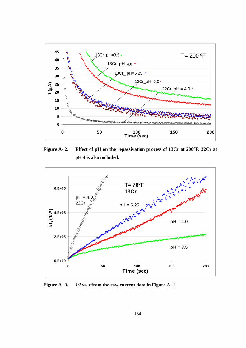
184
0
5
10
15
20
25
30
35
40
45
0 50 100 150 200Time (sec)
I( m
A)
22Cr_pH = 4.0
13Cr_pH=3.5 T= 200 ºF
13Cr_ pH=5.25
13Cr_pH=6.0
13Cr_pH=4.0
Figure A- 2. Effect of pH on the repassivation process of 13Cr at 200°F, 22Cr at
pH 4 is also included.
0.E+00
2.E+05
4.E+05
6.E+05
0 50 100 150 200
Time (sec)
1/I,
(1/A
)
T= 76ºF13Cr
pH = 3.5
pH = 4.0
pH = 5.25
pH = 4.022Cr
Figure A- 3. 1/I vs. t from the raw current data in Figure A- 1.

185
0.E+00
1.E+05
2.E+05
3.E+05
0 50 100 150 200Time (sec)
1/I,
(1/A
)
13Cr_pH=4.0
13Cr_pH=5.25
13Cr_pH=3.5
T= 200ºF
22 Cr,pH=4.0
13Cr_pH=6.0
Figure A- 4. 1/I vs. t from the raw data in Figure A- 2.
0
5
10
15
20
25
30
35
40
45
0 50 100 150 200Time (sec)
I( m
A)
T= 76ºF
Super13Cr_pH=3.50Super13Cr_pH=4.00Super13Cr_pH=5.25Super13Cr_pH=6.00
Figure A- 5. Effect of pH on the repassivation process of Super13Cr 76°F.

186
0
5
10
15
20
25
30
35
40
45
0 50 100 150 200Time (sec)
I( m
A)
Super13 Cr_pH=3.5
T= 200 ºF
Super 13Cr_ pH=5.25
Super 13Cr_pH=6.0
Super 13Cr_pH = 4.0
Figure A- 6. Effect of pH on the repassivation process of Super 13Cr at 200°F.
0.E+00
2.E+05
4.E+05
6.E+05
0 50 100 150 200Time (sec)
1/I,
(1/A
)
T= 76ºFSuper 13Cr
pH=3.5
pH=4.0pH=6.0
pH=5.25
Figure A- 7. 1/I vs. t from the raw data in Figure A- 5

187
0.E+00
1.E+05
2.E+05
3.E+05
4.E+05
0 50 100 150 200Time (sec)
1/I,
(1/A
) pH=4.0pH=5.25
pH=3.5
pH = 6T= 200ºFSuper 13Cr
Figure A- 8. 1/I vs. t from the raw data in Figure A- 6
Effect of type of material (CRA) on Scratch Test results
0
5
10
15
20
25
30
35
40
45
0 50 100 150 200Time (sec)
I( m
A)
T= 76ºF
Super _13Cr3.5 pH 6
13Cr_pH=4.00
13Cr_pH=5.25
22Cr_pH=4.00
13Cr_pH=3.50
Super13Cr_pH=3.50Super13Cr_pH=4.00Super13Cr_pH=5.25Super13Cr_pH=6.00
Figure A- 9. Comparison of the repassivation process of 13Cr and Super 13Cr at
76°F, 22Cr at pH 4 and room temperature is also included.
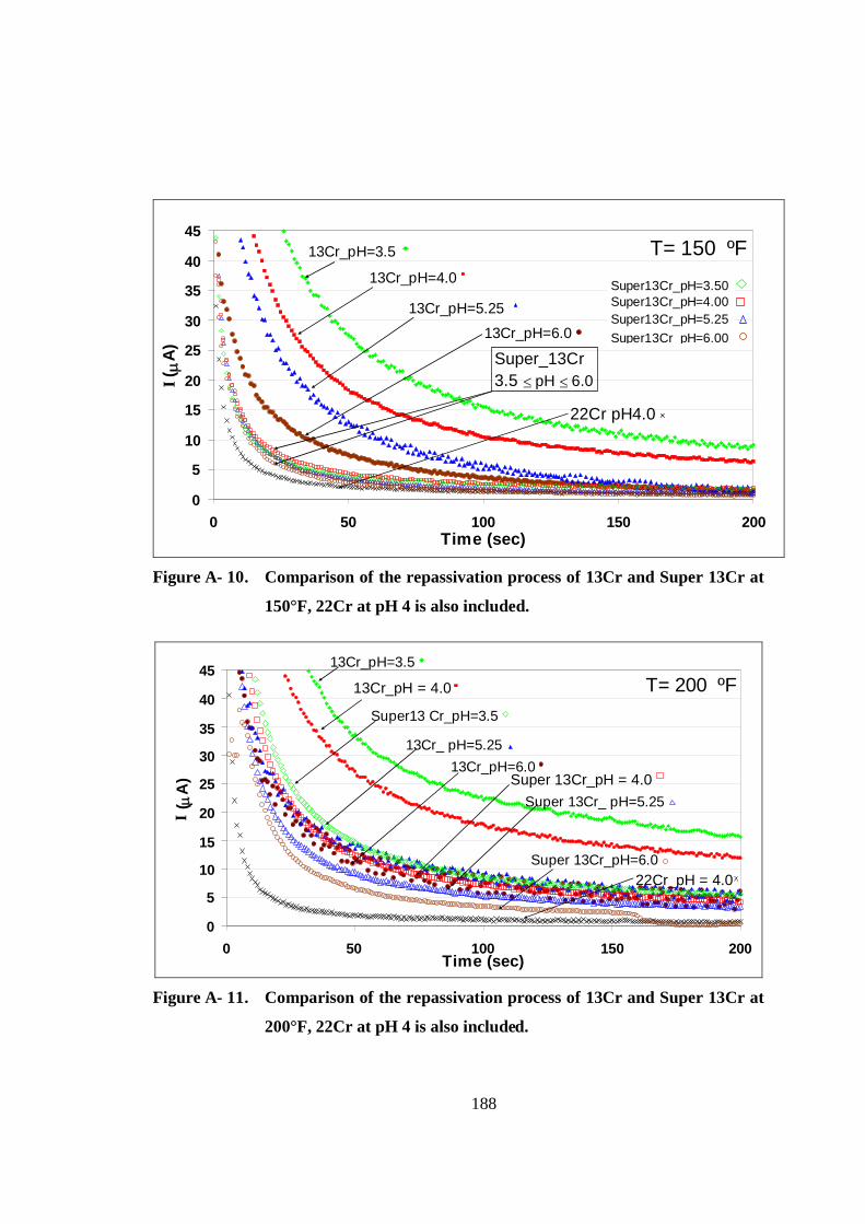
188
0
5
10
15
20
25
30
35
40
45
0 50 100 150 200Time (sec)
I( m
A)
T= 150 ºF13Cr_pH=3.5
13Cr_pH=4.0
13Cr_pH=5.25
13Cr_pH=6.0
22Cr pH4.0
Super_13Cr3.5 pH 6.0
Super13Cr_pH=3.50Super13Cr_pH=4.00Super13Cr_pH=5.25Super13Cr_pH=6.00
Figure A- 10. Comparison of the repassivation process of 13Cr and Super 13Cr at
150°F, 22Cr at pH 4 is also included.
0
5
10
15
20
25
30
35
40
45
0 50 100 150 200Time (sec)
I( m
A)
T= 200 ºF
22Cr_pH = 4.0
13Cr_pH=3.5
13Cr_ pH=5.25
13Cr_pH=6.0
13Cr_pH = 4.0
Super13 Cr_pH=3.5
Super 13Cr_ pH=5.25
Super 13Cr_pH=6.0
Super 13Cr_pH = 4.0
Figure A- 11. Comparison of the repassivation process of 13Cr and Super 13Cr at
200°F, 22Cr at pH 4 is also included.

189
0.E+00
2.E+05
4.E+05
6.E+05
0 50 100 150 200Time (sec)
1/I
,(1/
A)
T= 76ºF
13Cr_pH=3.5
13Cr_pH=4.0
Super13CrpH=5.25
Figure A- 12. Comparison of 1/I vs. t for 13Cr and Super 13Cr at 76°F, 22Cr at pH
4 is also included.
0.E+00
1.E+05
2.E+05
3.E+05
4.E+05
0 50 100 150 200Time (sec)
1/I,
(1/A
)
13Cr_pH=4.0
13Cr_pH=5.25
13Cr_pH=3.5
Super13Cr_pH=6.0
T= 200ºF
22 Cr,pH=4.0
Super13Cr_pH=5.25Super13Cr_pH=4.00Super13Cr_pH=3.50
13Cr_pH=6.0
Figure A- 13. Comparison of 1/I vs. t for 13Cr and Super 13Cr at 200°F, 22Cr at pH
4 is also included.
22Cr
pH=4
.0Sup
er13
Cr pH=6.0
Super 13Cr pH
=4.0Sup
er 13Cr pH=3.5
13Cr pH=5.25
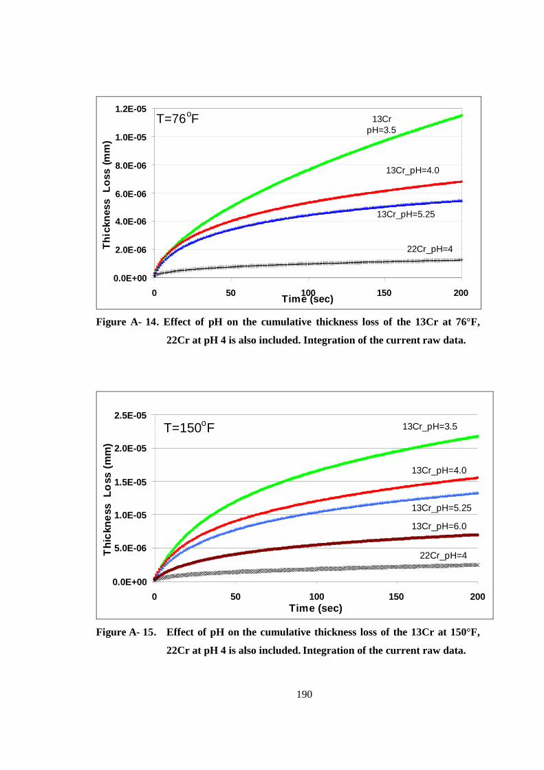
190
0.0E+00
2.0E-06
4.0E-06
6.0E-06
8.0E-06
1.0E-05
1.2E-05
0 50 100 150 200Time (sec)
Th
ickn
ess
Lo
ss(m
m)
T=76oF
22Cr_pH=4
13CrpH=3.5
13Cr_pH=4.0
13Cr_pH=5.25
Figure A- 14. Effect of pH on the cumulative thickness loss of the 13Cr at 76°F,
22Cr at pH 4 is also included. Integration of the current raw data.
0.0E+00
5.0E-06
1.0E-05
1.5E-05
2.0E-05
2.5E-05
0 50 100 150 200Time (sec)
Th
ickn
ess
Lo
ss(m
m)
T=150oF 13Cr_pH=3.5
22Cr_pH=4
13Cr_pH=4.0
13Cr_pH=5.25
13Cr_pH=6.0
Figure A- 15. Effect of pH on the cumulative thickness loss of the 13Cr at 150°F,
22Cr at pH 4 is also included. Integration of the current raw data.

191
0.0E+00
1.0E-05
2.0E-05
3.0E-05
4.0E-05
5.0E-05
6.0E-05
0 50 100 150 200
Time (sec)
Thic
kne
ssL
oss
(mm
)
13Cr_pH=3.5
13Cr_pH=4.0
13Cr_pH= 6.0
T=200oF
22Cr_pH=4
Figure A- 16. Effect of pH on the cumulative thickness loss of the 13Cr at 200°F,
22Cr at pH 4 is also included. Integration of the current raw data.
0.0E+00
1.0E-06
2.0E-06
3.0E-06
4.0E-06
5.0E-06
0 50 100 150 200Time (sec)
Th
ickn
ess
Lo
ss(m
m)
T=76oF
22Cr_pH=4
13CrpH=3.5
13Cr_pH=4.0 13Cr_pH=5.25
Super13Cr_pH=3.5
Super 13Cr_pH=5.25
Super 13Cr_pH=6.0
Super13Cr_pH= 4.0
Figure A- 17. Comparison of the cumulative thickness loss of 13Cr and Super
13Cr at 76°F, 22Cr at pH 4 is also included. Integration of the
current raw data.

192
0.0E+00
2.0E-06
4.0E-06
6.0E-06
8.0E-06
1.0E-05
1.2E-05
1.4E-05
0 50 100 150 200Time (sec)
Th
ickn
ess
Los
s(m
m)
T=150oF
22Cr_pH=4
13CrpH=3.5
13Cr_pH=4.0 13Cr_pH=5.25
Super 13Cr_3.5≤pH≤6.0
13Cr_pH=6.0
Figure A- 18. Comparison of the cumulative thickness loss of 13Cr and Super
13Cr at 150°F, 22Cr at pH 4 is also included. Integration of the
current raw data.
0.0E+00
4.0E-06
8.0E-06
1.2E-05
1.6E-05
2.0E-05
0 50 100 150 200
Time (sec)
Thic
kne
ss
Loss
(mm
)
13Cr_pH=3.5 13Cr_pH=4.00
13Cr_pH=5.25 & 6.0
T=200oF
22Cr_pH=4
Super13Cr_pH=3.5 & 4
Super 13Cr_pH=5.25
Super 13Cr_pH=6
Figure A- 19. Comparison of the cumulative thickness loss of 13Cr and Super
13Cr at 200°F, 22Cr at pH 4 is also included. Integration of the
current raw data.

193
0
20
40
60
80
0 50 100 150 200Time (sec)
I( m
A)
pH = 4.013Cr_200oF
13Cr_150oF
13Cr_76oF
22Cr,200, 150 & 76 oF
Super 13Cr_ 76oF
Super 13Cr_200oF
Super 13Cr_ 150oF
Figure A- 20. Comparison of the current decays for 13Cr, Super 13Cr and 22Cr
alloys at pH 4.0 and three different temperatures.
0
20
40
60
80
100
0 50 100 150 200Time (sec)
I( m
A)
pH= 6.0
13Cr, T =200oF
13Cr, T =150oF
Super 13Cr, T =200oF
Super 13Cr, T =150oF
Super 13Cr, T =76oF
Figure A- 21. Comparison of the current decays for both 13Cr and Super 13Cr
alloys at pH 6.0 and three different temperatures.

194
pH=4.0
0.0E+00
5.0E-06
1.0E-05
1.5E-05
2.0E-05
0 50 100 150 200Time (sec)
Th
ickn
ess
Lo
ss(m
m)
13Cr_76oF
13Cr_150oF13Cr_200oF
22Cr_200,
150 & 76oF
Super 13Cr_200oF
Super 13Cr_150oFSuper 13Cr_76oF
Figure A- 22. Comparison of the cumulative thickness loss of 13Cr, Super 13Cr
and 22Cr at pH 4. Integration of the current raw data.
0.0E+00
2.5E-06
5.0E-06
7.5E-06
0 50 100 150 200Time (sec)
Th
ick
nes
sL
oss
(mm
)
pH=6.0 13Cr_150oF13Cr_200oF
Super 13Cr_200oF
Super 13Cr_150oF
Super 13Cr_76oF
Figure A- 23. Comparison of the cumulative thickness loss of 13Cr and Super 13Cr
at pH 6. Integration of the current raw data.
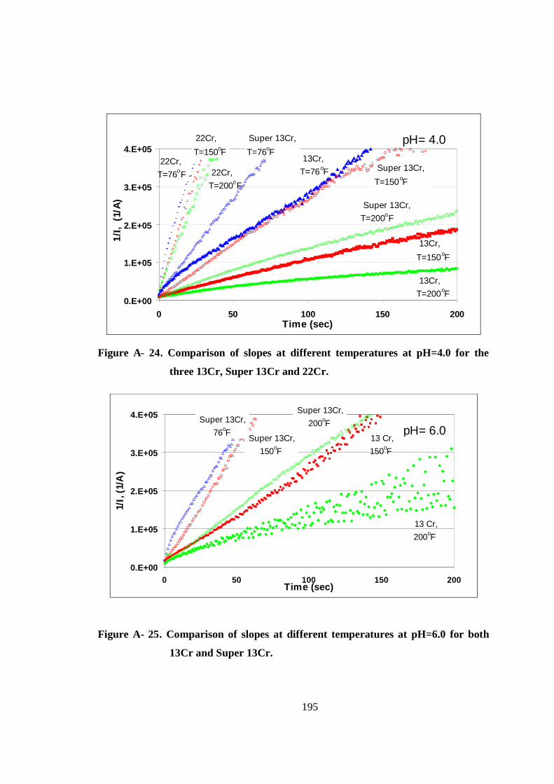
195
0.E+00
1.E+05
2.E+05
3.E+05
4.E+05
0 50 100 150 200Time (sec)
1/I,
(1/A
)
pH= 4.0
22Cr,T=200oF
13Cr,T=200oF
13Cr,
T=150oF
13Cr,T=76oF
22Cr,T=76oF
22Cr,
T=150oF
Super 13Cr,
T=76oF
Super 13Cr,
T=150oF
Super 13Cr,T=200oF
Figure A- 24. Comparison of slopes at different temperatures at pH=4.0 for the
three 13Cr, Super 13Cr and 22Cr.
0.E+00
1.E+05
2.E+05
3.E+05
4.E+05
0 50 100 150 200Time (sec)
1/I,
(1/A
)
pH= 6.0
13 Cr,200oF
13 Cr,150oF
Super 13Cr,76oF
Super 13Cr,150oF
Super 13Cr,200oF
Figure A- 25. Comparison of slopes at different temperatures at pH=6.0 for both
13Cr and Super 13Cr.

196
APPENDIX B
DETERMINATION OF THE “C” COSTANT
This appendix contents the mathematical analysis performed to obtain the
constant “C” used in the conversion of current to thickness loss per unit time for the three
CRAs.
From Faraday’s Law31 penetration rates can be obtained from equation (B-1)
provided that the corrosion current Icorr is known.
Penetration Raten
aiK (B-1)
Where, i = corrosion current density Icorr/exposed Area in A/cm2, = material
density in g/cm3, a = atomic weight, n = number of electrons lost (valence change). a/ n
is also known as Equivalent Weight, Weq and K is a conversion factor which changes
depending on the units required. K = 0.129 for mpy, 3.27 for m/y, 0.00327 for mm/y.
If the measured current in scratch test Imeasured is assumed to be Icorr, the constant
“C” used in equations (5-3), (5-5) and (5-6) in Chapter 5 is given by
A
WKC eq (B-2)
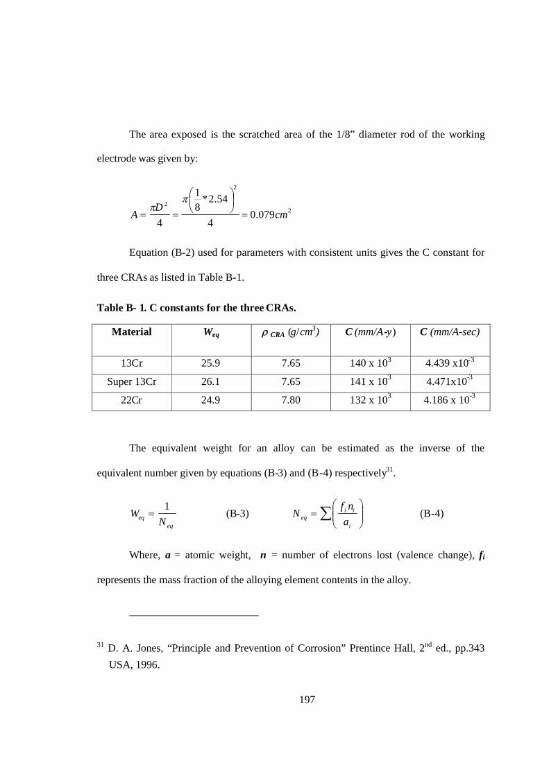
197
The area exposed is the scratched area of the 1/8” diameter rod of the working
electrode was given by:
2
2
2
079.04
54.2*81
4cm
DA
Equation (B-2) used for parameters with consistent units gives the C constant for
three CRAs as listed in Table B-1.
Table B- 1. C constants for the three CRAs.
Material Weq CRA (g/cm3) C (mm/A-y) C (mm/A-sec)
13Cr 25.9 7.65 140 x 103 4.439 x10⁻³
Super 13Cr 26.1 7.65 141 x 103 4.471x10⁻³
22Cr 24.9 7.80 132 x 103 4.186 x 10⁻³
The equivalent weight for an alloy can be estimated as the inverse of the
equivalent number given by equations (B-3) and (B-4) respectively31.
eqeq N
W1
(B-3)
i
iieq a
nfN (B-4)
Where, a = atomic weight, n = number of electrons lost (valence change), fi
represents the mass fraction of the alloying element contents in the alloy.
31 D. A. Jones, “Principle and Prevention of Corrosion” Prentince Hall, 2nd ed., pp.343
USA, 1996.

198
APPENDIX C
EROSION-CORROSION OF 13Cr EXPOSED TO VERY SEVERE
EROSIVITY CONDITIONS
Black coating development on 13Cr
An interesting phenomenon was observed when longer periods of time were
used to test 13Cr alloy at severe conditions such a direct impingement, low pH, high
flow velocities, and high sand rates. At such aggressive conditions, high current
magnitudes were obtained as seen in Figure C-1. The high current values were
sustained even after removing the sand, therefore the second order repassivation did
not result, and a black coating grew on the surface of the 13Cr target.
0
25
50
75
100
125
150
175
200
22 22.5 23 23.5 24 24.5 25 25.5 26
Time (hours)
I(m
A)
13Cr, pH 4, 150oF20 ft/s, 200 kg/day
Flow
ImpingementDirect
Figure C-1. Current response for 13Cr exposed to very severe erosivityconditions.

199
An effort to characterize the black coating was performed by means of
scanning electronic microscope (SEM), energy dispersive spectroscopy (EDS) and X-
ray diffraction (XRD). Figure C-2a shows the black coating grown on the metallic
surface of the 13Cr target specimen exposed to very severe erosion-corrosion
conditions (pH = 4.3, 150oF, 20ft/s, 200 Kg sand/day, more than 48 hours exposure).
a) 13Cr, pH4.3 long sand exposure b) SEM image of developed blackcoating 1000X
c) EDS of developed black coatingd) SEM image of developed black
coating 200X
Figure C-2. Black coating on metallic surface of the 13Cr target specimenexposed to erosion-corrosion conditions (pH = 4.3, 150oF, 20ft/s,200 Kg sand/day, more than 48 hours exposure).
The black coating seems to be scaly with a rough and cracked texture and
evenly distributed over the complete surface as seen on Figure C-2b and Figure C-2d.

200
The stoichiometry of the compound or compounds present in the black coating could
not be determined with the techniques used in this investigation, however the EDS
shown in Figure C-2c suggests it to be either a mixture of iron oxide and chromium
oxide or a Fe-Cr binary complex oxide. There are always chances for the corrosion
products to be hydrates types of compounds while they are still exposed to the wet
corrosive conditions, and then become de-hydrates oxides compounds showing
cracked texture due to shrinking during the dehydration process, similar to that
observed on Figure C-2b. Of course cracking could come from the continued particle
impingement on the brittle oxide layer.
Figure C-3a shows the metallic surface of the 13Cr target specimen exposed
to very severe erosion-corrosion conditions but for a short sand exposure time (pH =
4.3, 150oF, 20ft/s, 200 Kg sand/day, less than 10 minutes exposure). A pattern with
alternate rings was developed on the surface of the 13Cr. The pattern suggests an
incipient stage of the back coating development. The pattern suggests that the
erosion-corrosion damage is not uniform. Those regions were the erosion-corrosion
damage is greater the black coating grows earlier as a direct consequence of the
severity of the chemi-mechanical degradation process.
Figure C-3b shows a SEM image for the inner dark ring shown in Figure C-
3a. Numerous incipient pits with irregular shapes and a variety of sizes (up to 20
micrometers) can be seen along with some scratch marks from the polish preparation
process. Figure C-3c shows the EDS spectrum for the incipient black coating with the
same elements seen for the developed black coating. However, the intensity of the

201
peaks is different, indicating enrichment of Cr and O in the completely developed
black coating as compare with its incipient stage.
a) 13Cr, pH4.3 short sandexposure b) SEM image of incipient black
coating 1000X
c) EDS of incipient black coating
Figure C-3. Black coating patterns on metallic surface of the 13Cr targetspecimen exposed to erosion-corrosion conditions (pH = 4.3, 150oF,20ft/s, 200 Kg sand/day, less than 10 minutes exposure).
For erosivity conditions similar to those for which the black coating was able
to develop, but at the higher pH of 6, the black coating was inhibited and the passive
film reformed preventing high erosion-corrosion rates for 13Cr. Figure C-4 shows the
resultant metallic surface of 13Cr exposed to severe erosion-corrosion conditions and
pH = 6. The surface is dull but the black coating is not seen. The SEM image seen in
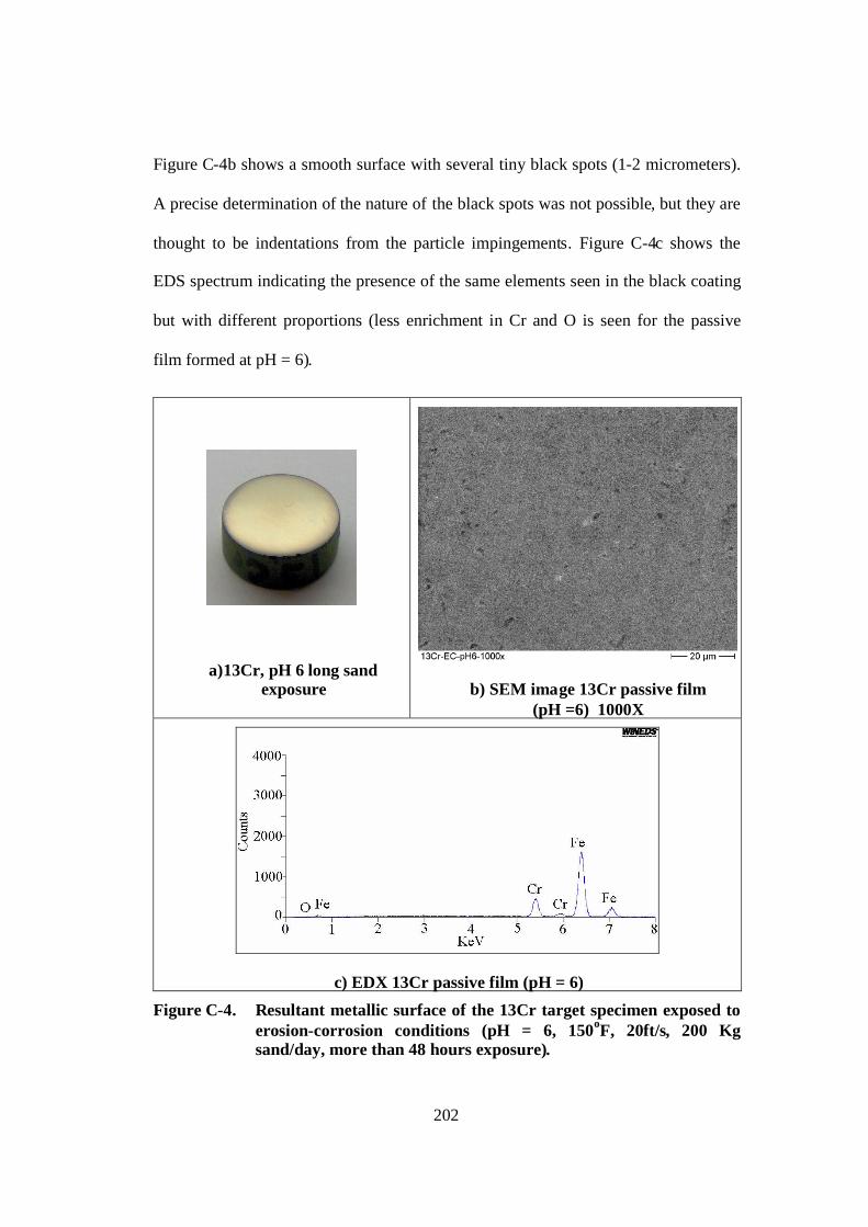
202
Figure C-4b shows a smooth surface with several tiny black spots (1-2 micrometers).
A precise determination of the nature of the black spots was not possible, but they are
thought to be indentations from the particle impingements. Figure C-4c shows the
EDS spectrum indicating the presence of the same elements seen in the black coating
but with different proportions (less enrichment in Cr and O is seen for the passive
film formed at pH = 6).
a)13Cr, pH 6 long sandexposure b) SEM image 13Cr passive film
(pH =6) 1000X
c) EDX 13Cr passive film (pH = 6)
Figure C-4. Resultant metallic surface of the 13Cr target specimen exposed toerosion-corrosion conditions (pH = 6, 150oF, 20ft/s, 200 Kgsand/day, more than 48 hours exposure).
203
Super 13Cr was also tested at erosivity conditions similar to those for which
the black coating was able to develop for 13Cr. Differences between 13Cr and Super
13Cr at these conditions were dramatic. The Super 13Cr showed lower current
magnitudes and second order behavior on repassivation with quick reformation of
passive film at pH of 4.3, resulting in significantly lower erosion-corrosion damage as
compared to 13Cr. Figure C-5 shows the resultant metallic surface of Super 13Cr
exposed to severe erosion-corrosion conditions and pH = 4.3. The surface is very
polished and bright as a mirror surface. The SEM image seen in Figure C-5b shows a
very smooth surface with several tiny darker spots (1-2 micrometers), thought to be
indentations from the particle impingements. Figure C-5c shows the EDS spectrum
indicating the presence of the same elements seen in the passive film of 13Cr but with
different proportions, and in addition, Nickel and Molybdenum peaks are present.
So far differences between the resultant surfaces for 13Cr and Super 13Cr
exposed to different conditions have been described, but the stoichiometric chemical
composition was not determined.
Furthermore, the black coating on the 13Cr was found to be rich in Fe and Cr,
similar to that found in the passive film of the same alloy. In fact no significant
distinction was seen between the spectrums obtained from the X-ray diffraction
analysis performed over the surfaces of the black coating and passive film of a 13Cr
as seen in Figure C- 6.

204
a)Super 13Cr, pH 4.3 long sandexposure b) SEM image Super 13Cr passive film
(pH =4.3) 1000X
c) EDX Super 13Cr passive film (pH = 4.3)
Figure C-5. Resultant metallic surface of the Super 13Cr target specimenexposed to erosion-corrosion conditions (pH = 4.3, 150oF, 20ft/s,200 Kg sand/day, more than 48 hours exposure).
However differences between the black coated 13Cr surface and the air-
passivated 13Cr surface in color, texture and appearance as observed without sight
aid devices as well as through SEM images clearly suggest significant distinctions

205
between the two surfaces. Furthermore, significant differences in the magnitudes of
the current obtained when the black coating is developed as opposed to when the
passive film is reformed, also suggest that the protective properties of the black
coating and the passive film are dramatically different. Thus, a carefully study to
better characterize the link between the erosion-corrosion response of 13Cr with its
surface finish is advised.
Figure C- 6. X-ray diffraction analysis on the black coating grown on a 13Crexposed to erosion corrosion-conditions and a on a air-passive13Cr surface.
Researchers 1,2 have successfully used X-ray Photoelectron Spectroscopy
(XPS) to characterize the passive films of CRAs. Results from this technique are
precise enough to determine the presence of distinguishable multilayers of oxides and

206
hydroxides with thicknesses from 1 to 5 nanometers depending upon the conditions at
which the passive films were formed. Olefjord and Wegrelius1 studied the passive
film of a stainless steel (20Cr18Ni6Mo0.2N) during polarization in 0.1 M HCl + 0.4
M NaCl. The film had two layers, an outer monolayer of Cr(OH)3 and a thicker inner
layer of Fe-Cr oxide.−Mo6+ and Mo4+ were also found enriched in the outer layer,
and their concentration depended on the potential. Ni2+ was also found in the passive
film but at very low concentration.
Vayer et. al. studied the effect of an HNO3 passivation treatment on the
characteristics of the passive film as compared to an air-passivated martensitic
stainless steel (X20Cr13, X30Cr13, X40Cr14). The HNO3 passivated film consisted
of a 3 nanometers thick layer with enhanced pitting resistance, and with oxidized
chromium and iron uniformly distributed, but enriched with oxidized chromium
(about 50% of the metallic elements of the passive layer was Cr). The air-formed
passive film consisted of a 4-5 nanometer double layer oxidized iron was
concentrated at the surface outer layer, and oxidized chromium was concentrated at
the inner layer closer to the metal matrix.
In summary, preliminary characterization of the black coating obtained for
13Cr exposed to certain very severe erosion-corrosion conditions was performed by
means of several techniques and it is known to be rich in Fe and Cr, suggesting it is a
combined Fe-Cr oxide. However, the exact chemical composition and crystalline
structure has not yet been clearly determined, and more research needs to be done in
this matter (XPS technique is advised to be used thoroughly for this purpose).

207
Potentiodynamic Scans for 13Cr and Super 13Cr Exposed to Corrosion
and Erosion-Corrosion Conditions.
A few potentiodynamic scans directed towards the understanding of
differences between the erosion-corrosion behavior of 13Cr and Super 13Cr were
performed. The liquid/sand flow loop (Microloop) was not provided with a
commercial reference electrode, therefore a rigorous analysis of the potential
parameters such as primary passivation potential Epp and corrosion potential Ecorr was
not performed. However, interesting results regarding the critical current density, icrit
and passive current density ip were obtained. Potentiodynamic scans are shown as a
function of the overpotential.
Figure C-7 shows potentiodynamic scans for 13Cr and Super 13Cr exposed to
brine flowing at 17 ft/s with a temperature of 150oF and pH = 4.3. Both alloys show a
broad passive range with low current. The larger passive range and lower passive
current density displayed by Super 13 Cr once again corroborate the better corrosion
resistance of this alloy as compare to 13Cr.
Figure C-8 shows potentiodynamic scans for Super 13Cr exposed to sand-free
brine and brine containing sand flowing at 17 ft/s with a temperature of 150oF and pH
= 4.3. Curves are similar at these conditions. Both shown a similar passive range,
however the passive current obtained with sand is about one half order of magnitude
larger than the curve obtained for sand free conditions.

208
Figure C-9 shows potentiodynamic scans for 13Cr exposed to sand-free brine
and brine containing sand flowing at 17 ft/s with a temperature of 150oF and pH =
4.3. The curves are greatly different at these conditions −for the curve obtained with
sand, the passive range shrunk, and the passive current is about one order of
magnitude larger than the curve obtained for sand free conditions. In addition the
steady state corrosion potential Ecorr seems to become more negative, so the critical
current icrit and primary passivation potential Epp appeared in the scan plot suggesting
that requirements to achieved passivation are more demanding under sand flows at
tested conditions (see Figure 2-3 and Figure 2-4 in Chapter 2).
For comparison purposes Figure C-10 shows the potentiodynamic scans for
Super 13Cr and 13Cr exposed to a brine containing sand shown in Figure C-8 and
Figure C-9 respectively. Again the larger passive range and lower passive current
density shown by Super 13Cr exposed to CO2 saturated brine containing sand also
corroborate the better erosion-corrosion resistance of this alloy as compare to 13Cr.

209
-100
0
100
200
300
400
500
600
1.E-09 1.E-08 1.E-07 1.E-06 1.E-05 1.E-04 1.E-03 1.E-02 1.E-01
Current Density, i (A/cm2)
Ov
erp
ote
nti
al
(mV
)
Super 13Cr Alloy 13Cr Alloy
No Sand, T = 150 oF, pH = 4.3, Vliq = 17 ft/s
Figure C-7. Potentiodynamic scans for 13Cr and Super 13Cr exposed to brineflow at 17 ft/s, 150oF and pH=4.3.
-100
0
100
200
300
400
500
600
1.E-09 1.E-08 1.E-07 1.E-06 1.E-05 1.E-04 1.E-03 1.E-02 1.E-01
Current Density, i (A/cm 2)
Ove
rpo
ten
tia
l(m
V)
No_Sand
Super 13Cr Alloy, T = 150 oF, pH = 4.3, Vliq = 17 ft/s
60 Kg/day of sand
Figure C-8. Potentiodynamic scans for Super 13Cr exposed to brine flow withand without sand at 17 ft/s, 150oF and pH=4.3.

210
-100
0
100
200
300
400
500
600
1.E-09 1.E-08 1.E-07 1.E-06 1.E-05 1.E-04 1.E-03 1.E-02 1.E-01
Current Density, i (A/cm2)
Ove
rpo
ten
tia
l(m
V)
No_Sand
13Cr Alloy, T = 150 oF, pH = 4.3, Vliq = 17 ft/s
60Kg/day of sand
i cri
E pp
Figure C-9. Potentiodynamic scans for 13Cr exposed to brine flow with andwithout sand at 17 ft/s, 150oF and pH=4.3.
-100
0
100
200
300
400
500
600
1.E-08 1.E-07 1.E-06 1.E-05 1.E-04 1.E-03 1.E-02 1.E-01
Current Density, i (A/cm2)
Ov
erp
ote
nti
al(
mV
)
60Kg/day of Sand, T = 150oF, pH = 4.3, Vliq = 17 ft/s
Super 13Cr Alloy13Cr Alloy
Figure C-10. Potentiodynamic scans for 13Cr and Super 13Cr exposed to brineflow with and without sand at 17 ft/s, 150oF and pH=4.3.

211
In summary potentiodynamic scans showed an anodic shift in the primary
passivation potential Epp along with the increment in the passive current density ipass,
for 13Cr exposed to the combined effects of high erosivity flows and severe
environmental conditions for the direct impingement testing. For these conditions
13Cr forms a black coating and repassivation is prevented. A more systematic
investigation into the conditions under which 13Cr will developed the black coating is
recommended along with more accurate characterizations of the chemical
composition and crystalline structure of the components of the black layer.
Potentiodynamics scans conducted for less severe flow conditions in a 13Cr
elbow flow geometry for similar environmental conditions showed a similar
increment in the passive current density ipass, but, the anodic shift in the primary
passivation potential Epp never occurred at these conditions3. For there conditions, no
black coating was observed and repassivation was accomplished. This suggests that
the requirements for repassivation might depend on the severity of flow conditions
and the erosivity level in addition to environmental conditions such pH, temperature
and chloride contents and water chemistry.
1 I. Olefjord and L. Wegrelius, Corrosion Science, Vol 31, pp. 89-98, 1990.
2 M. Vayer, I. Reynaud, and R. Erre, Journal of Material Science, Vol.35, pp.2581-2587, 2000.
3 Rincon, H.E. (2001). Erosion-Corrosion Phenomena of 13Cr Alloy in FlowsContaining Sand Particles, M.S. Thesis, Department of MechanicalEngineering, The University of Tulsa, Ok, Tulsa.

212
APPENDIX D
COMPUTATION FLUID DYNAMICS PROCEDURES
General Procedure
Erosion–Corrosion of metals by corrosive fluids carrying solid particles is a very
complex phenomenon present in several fields and industries. Research in this field is
very challenging due to the large amount of parameters affecting the degradation
mechanism.
During this research, an experimental approach has been adopted for the study of
many of these variables such as temperature, pH, material composition, material
properties and sand rates. Also, several flow velocities, flow patterns and flow geometries
have been experimentally tested to characterize the effect of such variables on the
erosion-corrosion damage of CRAs. However, the hydrodynamics of the conditions
tested are complex and additional tools are needed to better understand the degradation
mechanism. In addition, experiments to emulate field conditions are very difficult to
perform, expensive and time consuming. Thus, overall lack of predictability is
characteristic of these kinds of studies.
The contributions of computational fluid dynamics (CFD) to more closely
simulate the hydrodynamics of field conditions and to reduce data are encouraging.

213
Significant efforts have been directed towards the use of CFD as a potential tool to
evaluate and predict solid particle erosion. Some researchers have also included the
prediction of erosion-corrosion. The present work does not attempt to develop any new
CFD procedure. Here CFD is used as a tool to predict the hydrodynamics, particle
tracking, and erosion of a material exposed to a flowing slurry system since, erosion is a
necessary component of erosion-corrosion.
Several authors1-6 have followed the same general procedure to obtain the
numerical evaluation of erosion. The procedure can be summarized in three major steps:
1) generation and convergence of flow field domain simulation, 2) computation of the
stream particle trajectories inside the flow field, and 3) computation of the erosion rate by
applying the suitable erosion model equations. According to Bozzini et. al.,Error! Bookmark
not defined. two additional steps are required if the corrosion component needs to be
included. The additional steps are: 4) evaluation of the impact-induced corrosion effect
and 5) evaluation of the synergistic erosion-corrosion damage.
In this research, a semi-mechanistic model to predict erosion-corrosion of CRAs
has been developed and implemented based on the solid particle impingement
information collected from CFD simulations. The estimation of the impact-induced
corrosion and the synergistic effect of the erosion-corrosion damage have been included
in the model. Only the prediction of erosion rates is performed during the CFD
simulations, the impact-induced corrosion and erosion corrosion rates are not actually
executed during the CFD simulations but in a separate VBA (Visual Basic for
Applications) code built for that specific purpose.

214
This appendix briefly summarizes the complete CFD procedures used to predict
erosion rates and produce the solid particle impingement information needed as an input
for the erosion-corrosion prediction model. The impingement information includes, (x, y,
z) coordinates of the cell center (m), Cell Area (m2), total impact number in the cell,
averaged impact speed in a cell (m/s), averaged impact angle in a cell (degree), and
erosion (kg removed metal/m2.s).
Numerical Model Approach
CFD experts agree on the convenience of combining the Eularian CFD modeling
to predict the flow field on the continuous fluid phase with the Lagrangian particle
tracking of the solid or particulate phase2-5. Eularian modeling of the discrete phase is
also possible, however, the particle-wall interactions have been shown to be difficult to
manage.Error! Bookmark not defined.
The model presented here is Eularian-Lagrangian and can be broken down to the
following main steps: build and mesh geometry, fluid flow model, particle tracking
model, and erosion model.
CFD Geometry and Mesh
The geometry of the CFD model was built simulating features and dimensions of
the direct impingement test cell of the single phase liquid flow test whose schematic is
shown in chapter 4. Figure D- 1.a shows the CFD geometry as built with Gambit 2.1.6
software indicating the place of the jet and the target specimen.
215
A grid refinement study was performed to guarantee grid-size-independent
results. Several mesh designs were examined for good convergence of the solution and
reasonable computational time that did not compromise result quality.
Figure D- 1.b shows the exterior mesh grid use for the volume representing the
cross fitting. The biggest volume element size used for the simulation was 0.05% of the
total volume. For the interior of the volume, a size function along an imaginary
centerline, going from the center of the jet to the center of the target, was used to mesh
the entire volume. The size of the volume elements grew from a starting size of 0.005%
for those elements next to the center line, to a maximum size of 0.05% at a rate of 1.1%,
as shown in Figure D- 1.c. Figure D- 1.d shows the 2D elements for the face of the target
specimen. This face has a total of 684 computational cells with areas varying from 8.28E-
09 to 7.68E-07 m2, for a total area of 2.0E-4 m2 or 2 cm2 which matches the actual
impinged surface area of the specimen.
Flow Modeling
Flow simulations were accomplished by means of a commercially available
software (FLUENT version 6.1). First, flow fields were determined by using the kinetic
energy-dissipation rate (-) two-equation model of turbulence. This model is usually a
good starting point since it has been extensively used for several geometries with
reasonably good estimates of the flow field and relatively low computational time (easy
convergence). However, places where recirculation zones are expected may not be
completely resolved with this turbulence model. Hence, the Reynolds Stress Model
(RSM) was also used. Flow simulations obtained with both turbulence models were
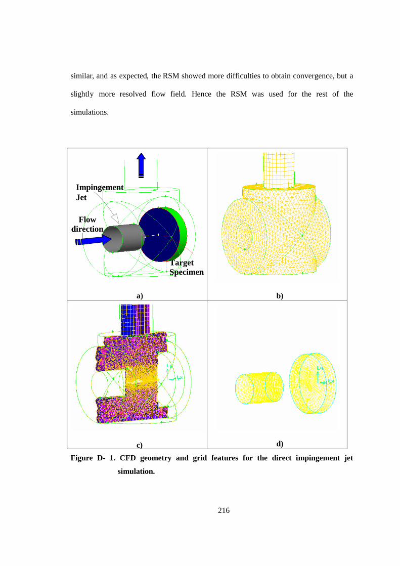
216
similar, and as expected, the RSM showed more difficulties to obtain convergence, but a
slightly more resolved flow field. Hence the RSM was used for the rest of the
simulations.
a) b)
c) d)
Figure D- 1. CFD geometry and grid features for the direct impingement jet
simulation.
Flowdirection
ImpingementJet
TargetSpecimen
Flowdirection
ImpingementJet
TargetSpecimen
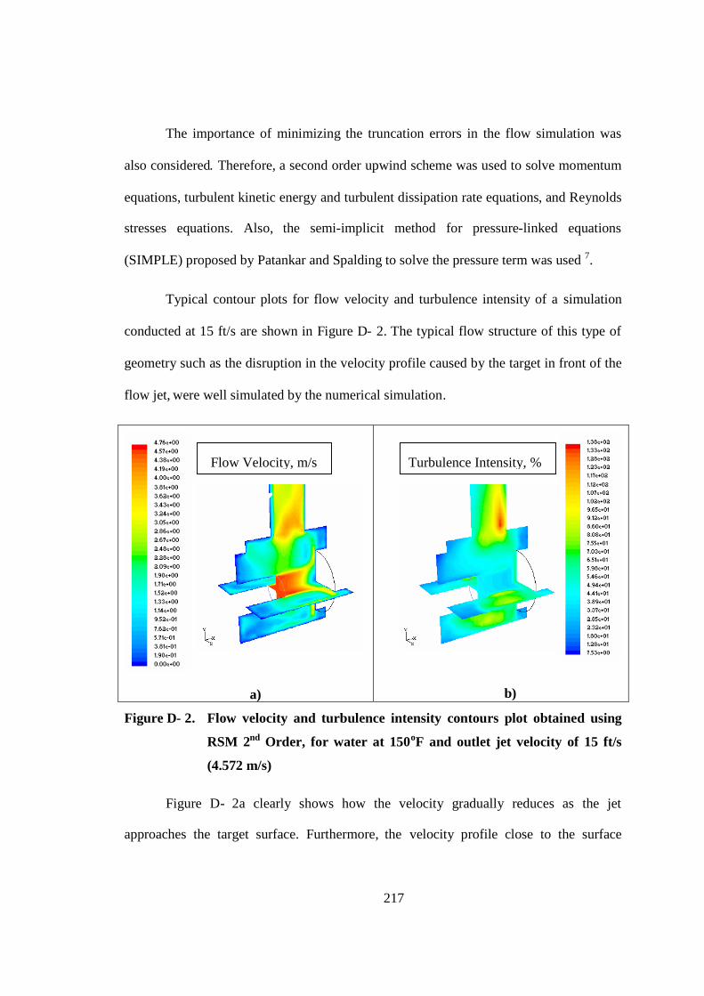
217
The importance of minimizing the truncation errors in the flow simulation was
also considered. Therefore, a second order upwind scheme was used to solve momentum
equations, turbulent kinetic energy and turbulent dissipation rate equations, and Reynolds
stresses equations. Also, the semi-implicit method for pressure-linked equations
(SIMPLE) proposed by Patankar and Spalding to solve the pressure term was used 7.
Typical contour plots for flow velocity and turbulence intensity of a simulation
conducted at 15 ft/s are shown in Figure D- 2. The typical flow structure of this type of
geometry such as the disruption in the velocity profile caused by the target in front of the
flow jet, were well simulated by the numerical simulation.
a) b)
Figure D- 2. Flow velocity and turbulence intensity contours plot obtained using
RSM 2nd Order, for water at 150oF and outlet jet velocity of 15 ft/s
(4.572 m/s)
Figure D- 2a clearly shows how the velocity gradually reduces as the jet
approaches the target surface. Furthermore, the velocity profile close to the surface
Flow Velocity, m/s Turbulence Intensity, %

218
suggests there is a low flow velocity zone at the center region of the target which has
been commonly referred to as a “stagnation zone”. Surrounding this zone, flow velocities
are still high and streamlines are radially diverted away form the center line, causing
reverse flows and secondary cross-flow vortices around the projected high flow velocity
jet.
Validation of the flow simulation by comparison with actual flow velocity profile
data was not explicitly done during this research. However, Yongli8 recently has
successfully compared simulations performed with the same numerical solution approach
to experimental data collected with a Laser Doppler Velocimetry (LDV) It was found that
the numerical simulation reasonably matched the experimental data.
Particle Tracking
As mentioned before, a Lagrangian approach was taken to conduct the particle
tracking. The equation of dispersed particle motion is essentially a force balance around a
single particle. FLUENT also has the capability to couple the particle equation of motion
with the flow solution. However, at low particle concentrations the particles do not affect
the flow and, thus, coupling is not necessary.
The particle motion comes from Newton’s second law of motion is expressed as:
dt
dVmF p
p D-(1)
where Vp is the particle velocity vector, mp, is the particle mass and F is the resultant
force vector on the particle which may include drag force, FD, exerted by the fluid on the
particle, buoyancy force, FB, due to differences in fluid–particle densities, pressure

219
gradient force, Fp, exerted by pressure gradients on the continuous phase, the added mass
force, FA, which accounts for the inertia of the fluid surrounding the particle (also named
as virtual mass force), the Saffman lift force and the rotating coordinates force, FR, which
accounts for rotational motion and centrifugal effects may contribute significantly to the
particle motion and were included in the particle simulation. Further details of the forces
included in the particle tracking, their mathematical representations and the physics
behind them have been extensively discussed in literature and a good summary may be
found in the user guide of FLUENT 7.
The effect of turbulence on the particle dispersion was also considered based on
the “random eddy lifetime” model to predict the turbulent dispersion of particles as
interacting with a series of fluid phase turbulent eddies. Also Grant and Tabakoff 9
correlations for the restitution coefficients required to predict particle velocity after
impact with a solid surface were included in the simulation.
Erosion Model
Most of currently available models predict erosion based on a direct impingement
mechanism. Many also include the effects of turbulent fluctuations and the random
impingement mechanisms10. In any case, results presented here are not expected to be
significantly affected by this, since erosion predictions were performed for direct
impingement flow geometry. In the direct impingement mechanism, the particles are
driven to the walls primarily by the momentum of the particle provided by mean flow
velocity. Where viscous effects are small or when the particles are large and dense as
compared with the carrier fluid density, direct impingements can be the dominant

220
mechanism. For denser liquids carrying sand, velocity fluctuations due to turbulence may
effect particle motion. Turbulent eddies can transfer radial momentum to the particles
near the wall and cause random impingements resulting in erosion damage; but, this
effect is expected to be small for direct impingement simulations.
If the impingement impact speed and angle are known, the erosion rate can be
computed. Erosion rates may be expressed in different units; most commons used units
are: penetration rate, which is the amount of wall thickness loss per unit time or amount
of mass loss per unit time. Other quantities of interest are erosion ratio, defined as the
amount of mass lost by the pipe wall due to erosion divided by the total mass of particles
impinging the metal.
Some of the erosion models available in the literature provide equations can be
broken down into 3 factor functions 1-3, 8-12 The first function accounts for the effect of
flow velocities and is usually the impact velocity raised to a power, with the power being
from 1.7 to 2.4. The second term refers to the effect of impact angle; this term usually
comes from fitted data obtained from direct impingement erosion tests conducted at
different impact angles. The last term usually accounts for properties of the erodent,
target material or even flow geometries.
Edwards et alError! Bookmark not defined. used relations provided by Ahlert 11 for
carbon steels, developed at The University of Tulsa. These relations depend primarily on
the particle impact speed and impact angle. As seen in the following equation:
fVAFER ns (D-2)

221
where Fs is a particle shape coefficient (Fs=1.0 for sharp (angular), 0.53 for semi-
rounded, or 0.2 for fully rounded sand particles). Ahlert11 used two functional forms of
the angle dependence, with matching conditions applied at some angle . The
dependence on impingement angle, f (), is given in Eqs. (D-3) and (D-4).
baf 2 for (D-3)
zyxf 22 sinsincos for (D-4)
A, a, b, , x, y, z, and n, are all empirical constants.
This model was developed based on direct impingement data obtained from gas-
sand flows testing, and tends to over-predict the estimated penetration rates. A more
recent work published by Oka et al.12 in 2005 uses correlative equations derived from
particle impact energy and indentation behavior as a function of material hardness to
generalize prediction of metal loss regardless of the target material. This model was also
first developed for gas-sand flows. However, it seems to grasp more of the physics
involved in the erosion process and has been successfully used by Yongli et al.8 to
estimate direct impingement erosion rates in liquids by means of CFD.
The Oka model12 assumes that erosion is mainly driven by the impact velocity,
impact angle, size and type of particles and material hardness. The general equation to
estimate material loss is given by equation (D-4):
90)()( EgE (D-4)

222
where, E() represents the removed material volume per mass of particle
(mm3/kg) at any angle ; E90 is the erosion damage at 90 degree angle and g() denotes
the function ratio of erosion ratio at any given angle E() to that at normal angle E90.
The angle function depends on the material hardness (Vickers Hardness, Hv in
Gpa) and accounts for what the authors12 referred to as a “repeated plastic deformation”
linked to the normal component of the impact velocity (first term in Equation D-5). A
“cutting action” proved to be more effective at low impact angles (second term in
equation D-5).
21 ))sin1(1()(sin)( nn Hvg (D-5)
where n1 and n2 are similar functions with constants determined experimentally which
accounts for material hardness and erodent properties. Functions n1 and n2 are given by
equation (D-6)
qHvSnn )(, 21 (D-6)
For sand particle Sn1= 0.71, qn1 = 0.14, Sn2= 2.4 and qn2 = -0.94.
The erosion damage at normal angle E90 has been discussed in detail by Oka and
Yoshida,13 and accounts for impact velocity, V(m/s), particle diameter, D(m), and
material hardness according to equation B-7 as follows.
32
1)(90
kkk
DD
VV
HvKE
(B-7)
where K, k1, k2 and k3 are constants determined experimentally. K and k1 depend on
particles properties, k2 depends on particle properties as well as on material hardness. For
223
sand K = 65, k1 = -0.12, k2 = 2.3(Hv)0.0038 and k3 = 0.19 regardless of the erodent used. V’
(104 m/s) and D’ (326 m) are reference velocity and particle diameter respectively used
in the experiments to obtain the correlations of the erosion damage.
In the numerical calculation of the metal mass loss it is assumed that when a
particle strikes the wall, the mass loss is distributed uniformly over the computational cell
in which the particle impinged. With both sufficiently small grid spacing and a large
number of particles simulated, approximation errors induced by this assumption can be
kept at a minimum.
Once all particle trajectories have been computed and all wall impingement data
gathered, the mass loss for all impingements can be compiled to generate a local
penetration rate for each cell that lies on the surface of the geometry. At grid cell j on the
surface of the geometry, the local Erosion penetration rate, Ecell(j), is given by:
i
ji
p
p
pj
pjcell E
NN
A
dE )(
)()(
3)(
6
(D-8)
where A(j)is the surface area of the computational cell j, E()i(j) denotes the erosion ratio of
impingement i at cell location j,
pN is the number of particles per second flowing, Np is
the total number of particles simulated, and p is the particle density.
CFD simulation sample cases
Table D- 1 shows the combination of flow velocities and sand rates used in the
CFD simulations to generate the solid particle information and erosion rates used as input
in the erosion-corrosion model proposed in this research. Flow velocities and sand rate

224
were selected to approximately match the experimental conditions used in the single
phase liquid flow loop.
Table D- 1 Flow velocity and sand rate combinations for simulations performed
in CFD for 13Cr and Super 13Cr materials.
Velocity(ft/s)
Velocity(m/s)
SandRate
(kg/day)10 3.05 1010 3.05 2510 3.05 10015 4.57 5515 4.57 16515 4.57 23517 5.18 6017 5.18 13220 6.10 6020 6.10 7520 6.10 10820 6.10 20020 6.10 400
As mentioned earlier, the Oka erosion model was based on gas-sand experimental
data tested at much higher flow velocities with higher erosion rates. Hence, some over-
prediction was expected from these simulations as compared to the experimental data
collected for liquid-sand direct impingement. However, impact velocities, impact angles,
and erosion patterns obtained in simulations are reasonable. The erosion pattern, impact
velocity profile and impact angle profile were similar for all simulations regardless of
sand rate and flow velocity, and typical simulation results are shown in Figure D- 3.

225
a) Impact Velocity (m/s) b) Impact Angle (degree)
c) Impact Hits (#/s) d) Erosion (mpy) Avg = 9.9 mpy
Figure D- 3. Impact velocity, impact angle and number of impacts and erosion rate
distributions for CFD simulation performed for 13Cr at 10 ft/s (3.048
m/s) and sand rate of 25 kg/day.

226
1 Edwards J., McLaury B., Shirazi S., “Evaluation of Alternative Pipe Bend Fittings
in Erosive Service”, Proceedings of Fluid Engineering Summer Meeting ASME
2000, June 11-15-2000, Boston, Massachusetts.
2 Edwards J., McLaury B., Shirazi S., “Modeling Solid Particle Erosion in Elbows
and Plugged Tee”, Journal of Energy Resources Technology, ASME, Vol 123,
December 2001.
3 Wallace M., Peters J., “CFD-Based Erosion Modelling of Multi-Orifice Choke
Valves”., Proceedings of Fluid Engineering Summer Meeting ASME 2000, June
11-15-2000, Boston, Massachusetts.
4 Keating, A. and S. Nesic (2000). "Particle Tracking and Erosion Prediction in
Three-Dimensional Bends", Proceedings of Fluid Engineering Summer Meeting
ASME 2000, June 11-15-2000, Boston, Massachusetts.
5 Bozzini, B., M. E. Ricotti, et al. (2003). "Evaluation of erosion-corrosion in
multiphase flow via CFD and experimental analysis." Wear 255(1-6): 237-245.
6 Keating, A. and S. Nesic (2001). "Numerical prediction of erosion-corrosion in
bends." Corrosion 57(7): 621-633.
7 User’s Guide,Fluent 6.1 Documntation.
227
8 Yongli Zhang, Erik Reuterfors, Brenton S. McLaury, Siamack A. Shirazi, and
Edmund F. Rybicki. “Experimental and CFD results for particle velocities and
erosion.” Submitted to Wear journal
9 Grant G. and Tabakoff W., “Erosion Prediction in Turbomachinery Resulting from
Environmental Solid Particles,” J. Aircraft, Vol. 12, No. 5, pp. 471-478
10 Edwards, J., Development, Validation, and Application of a Three-Dimensional,
CFD-Based Erosion Prediction Procedure, PhD Dissertation, Department of
Mechanical Engineering, The University of Tulsa, 2000.
11 Alhert, K., Effects of Particle impingement Angle and Surface Wetting on Solid
Particle Erosion of AISI 1018 Steel, M.S. Thesis, Department of Mechanical
Engineering, The University of Tulsa, 1994.
12 Oka, Y.I, Okamura, K., Yoshida, T., “Practical estimation of erosion damage
caused by solid particle impact. Part 1: Effects of impact parameters on a predictive
equation.” Wear 259 (95-101)
13 Oka, Y.I, Yoshida, T., “Practical estimation of erosion damage caused by solid
particle impact. Part 2: Mechanical properties of materials directly associated with
erosion damage.” Wear 259 (102-109)
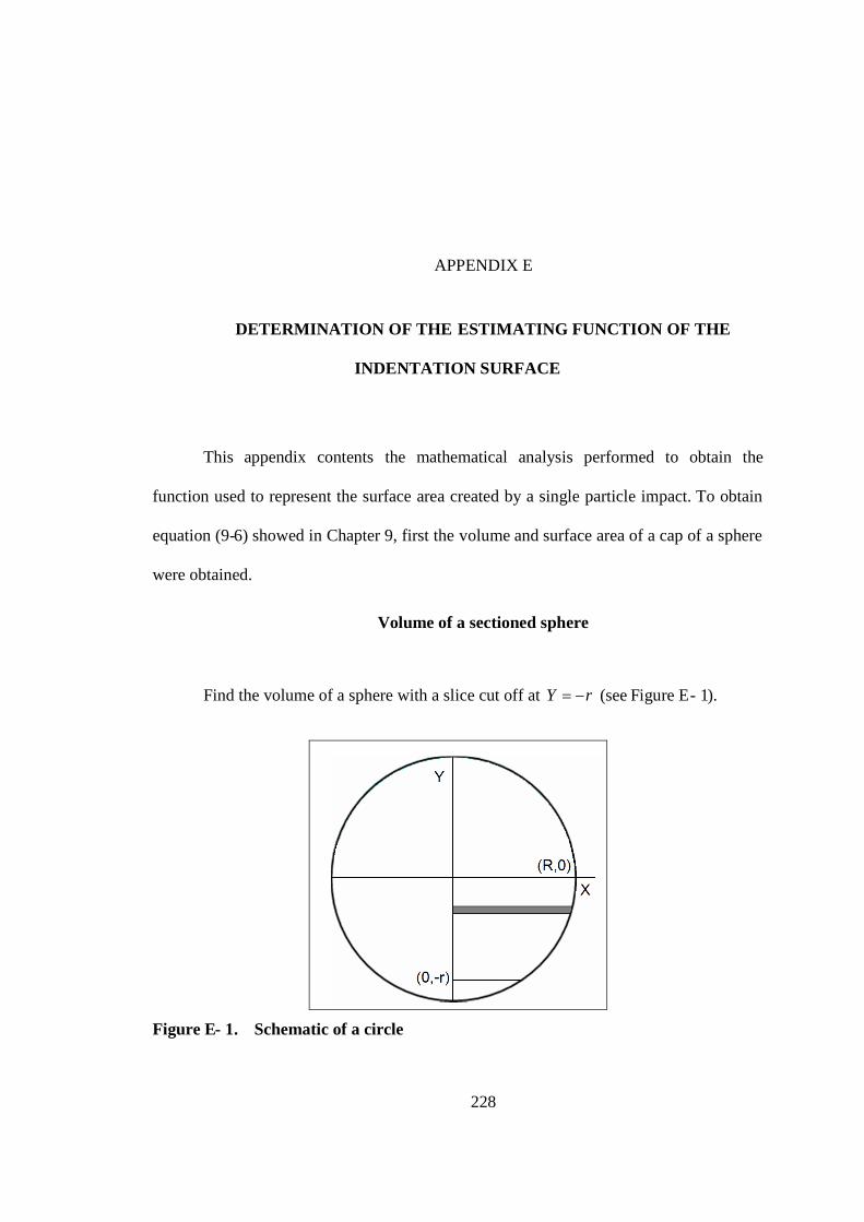
228
APPENDIX E
DETERMINATION OF THE ESTIMATING FUNCTION OF THE
INDENTATION SURFACE
This appendix contents the mathematical analysis performed to obtain the
function used to represent the surface area created by a single particle impact. To obtain
equation (9-6) showed in Chapter 9, first the volume and surface area of a cap of a sphere
were obtained.
Volume of a sectioned sphere
Find the volume of a sphere with a slice cut off at rY (see Figure E- 1).
Figure E- 1. Schematic of a circle

229
The volume of the hemisphere above the X axis is ½ the volume of the sphere
33
32
34
21
RRVhemisphere
(E-1)
Below the X axis, the value of dV is the area of a disk 2X times the
infinitesimal height dY
dYXdV 2 (E-2)
From equation of circle 222 RYX
Hence the volume for the section from Y= –r to Y = 0 is given by.
03
020 22
3r
rr
YYRdYYRV
(E-3)
332 03
0 rrRV (E-4)
33
3232 rrRrrRV
(E-5)
The crater volume is the total volume of the sphere below rY or the volume
of the hemisphere minus equation (E-5) given by.
332
332 3
233
23 rrRR
rrRRVcrater
(E-6)
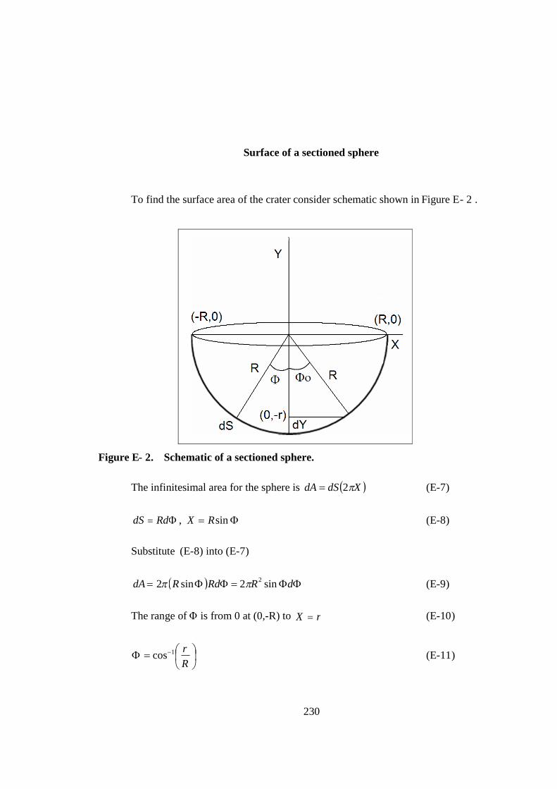
230
Surface of a sectioned sphere
To find the surface area of the crater consider schematic shown in Figure E- 2 .
Figure E- 2. Schematic of a sectioned sphere.
The infinitesimal area for the sphere is XdSdA 2 (E-7)
RddS , sinRX (E-8)
Substitute (E-8) into (E-7)
dRRdRdA sin2sin2 2 (E-9)
The range of Φis from 0 at (0,-R) to rX (E-10)
Rr1cos (E-11)

231
The integral is
Rr
Rr
RdRdAA1 1cos
0
cos
022 cos2sin2 (E-12)
0coscoscos2 12
Rr
RA (E-13)
RrR
RrRA 1212 22 (E-14)
Where r < R.
The questions are:
(1) What is the ratio of the volume below rY , Vcrater, to the sphere volume,
Vsphere?
(2) What is the ratio of the surface area of the sphere below rY , Acrater, to the total
surface volume of the sphere, Asphere?
Answer (1)
3
3
3
323
332
43
34
31
32
Rr
Rr
R
rrRR
VV
sphere
crater
(E-15)
Answer (2)
Rr
RRrR
REq
AA
sphere
crater 121
4
12
418
2
2
2
(E-16)

232
Area Ratio to Volume Ratio Relationship
To obtain equation (9-6) showed in Chapter 9, a regression was made with data
generated from equations (E-15 and E-16). Figure E- 3 shows the fitted curve for the
Area Ratio to Volume Ratio relationship. As can be seen the fitted curve does a very
good match with data generated from equations (E-15 and E-16), for a broad range of
volume ratios, meaning that this relationship can be used for a broad range of erosion
ratios. Typical erosion ratios for a single particle impingement of liquid flows containing
sand are within 10-9 and 10-12 while for gas flows containing sand erosion ratios may fall
within 10-8 to 10-6. Hence this relationship will cover the whole range of erosion ratios
with accuracy.
1.E-07
1.E-06
1.E-05
1.E-04
1.E-03
1.E-02
1.E-01
1.E+00
1.E-12 1.E-10 1.E-08 1.E-06 1.E-04 1.E-02 1.E+00
Vcrater/Vsphere
Acr
ater
/Asp
he
re
Acrater/Asphere= 0.6022 (Vcrater/Vsphere)^0.5026
Figure E- 3. Area ratio to volume ratio relationship.

233
APPENDIX F
VBA CODE FOR THE PROPOSED EROSION-COROSION MODEL
Sub Erosion-Corrosion Model()
'Estimation of the Total current, Corrosion Component Rates and Erosion-CorrosionRates PER EACH CFD NUMERICAL CELL of CRAs in CO2 Saturated BrineContaining Sand
Dim Time(100000, 1) As Double, Dim I(100000) As Double, DimI_high(100000) As Double, Dim I_low(100000) As Double, Dim I_Avg(100000) AsDouble, Dim I_cum(100000) As Double, Dim pi As Double, Dim Part_flow AsDouble, Dim Name_Input_File As String, Dim TotalCell As Integer, Dim FinalWBAs Workbook, Dim AvgInfoWS As Worksheet, Dim QuickCalcSheet As Worksheet
'Reading Input from Source Code WorkBook "QuickCalc Spreadsheet"
m_st = Worksheets("QuickCalc").Cells(2, 2) '1/A*sec
Io_st = Worksheets("QuickCalc").Cells(3, 2) 'microA
Stop_Current = Worksheets("QuickCalc").Cells(4, 2)
D_part = Worksheets("QuickCalc").Cells(2, 4) 'micrometer
f = Worksheets("QuickCalc").Cells(3, 4) 'Kg/m^3
rho_sand = 2650 'Kg/m^3
material = Worksheets("QuickCalc").Cells(1, 24)
Simulated_particles = Worksheets("QuickCalc").Cells(3, 6)
Sand_rate = Worksheets("QuickCalc").Cells(4, 6) 'Kg/day
I_vs_time_info = Worksheets("QuickCalc").Cells(1, 27)
Plots = Worksheets("QuickCalc").Cells(1, 30)
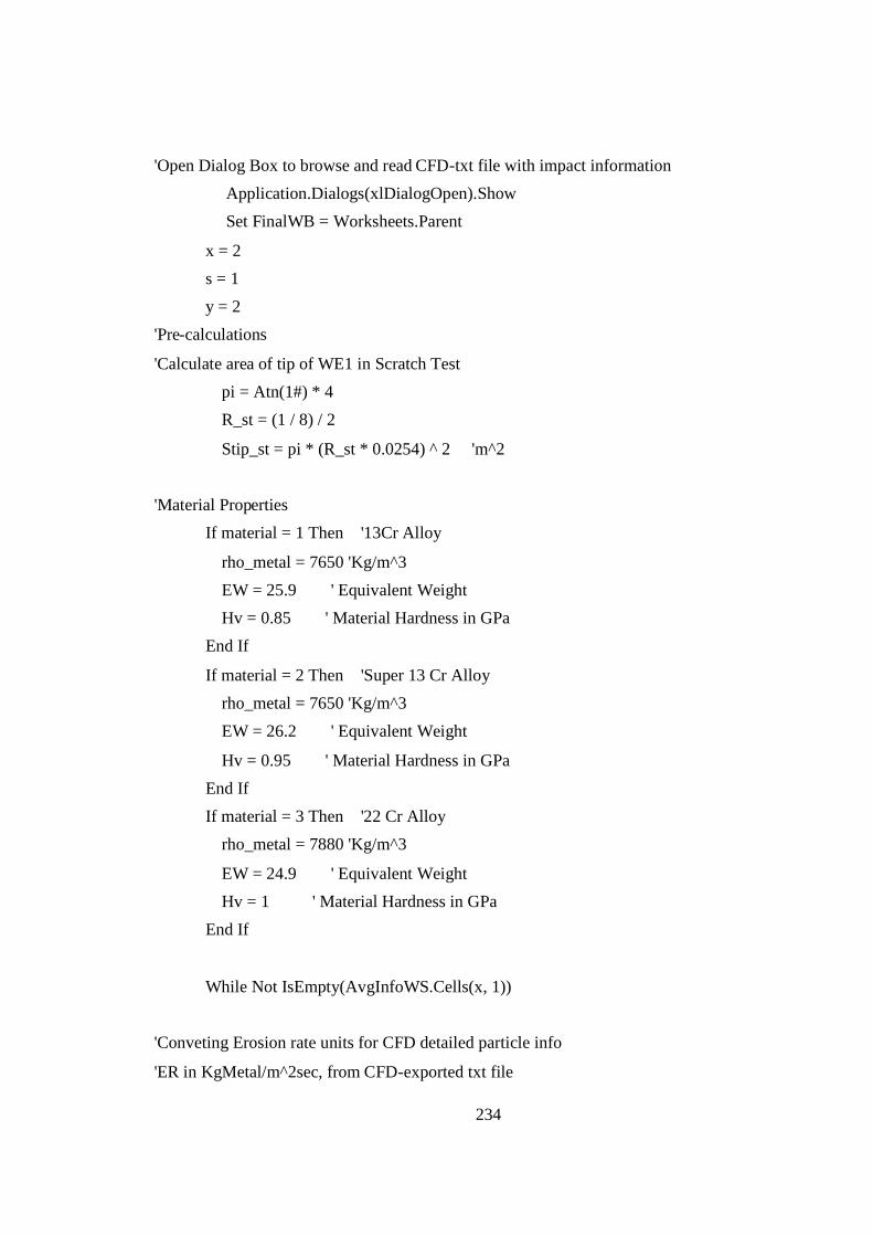
234
'Open Dialog Box to browse and read CFD-txt file with impact information
Application.Dialogs(xlDialogOpen).Show
Set FinalWB = Worksheets.Parent
x = 2
s = 1
y = 2
'Pre-calculations
'Calculate area of tip of WE1 in Scratch Test
pi = Atn(1#) * 4
R_st = (1 / 8) / 2
Stip_st = pi * (R_st * 0.0254) ^ 2 'm^2
'Material Properties
If material = 1 Then '13Cr Alloy
rho_metal = 7650 'Kg/m^3
EW = 25.9 ' Equivalent Weight
Hv = 0.85 ' Material Hardness in GPa
End If
If material = 2 Then 'Super 13 Cr Alloy
rho_metal = 7650 'Kg/m^3
EW = 26.2 ' Equivalent Weight
Hv = 0.95 ' Material Hardness in GPa
End If
If material = 3 Then '22 Cr Alloy
rho_metal = 7880 'Kg/m^3
EW = 24.9 ' Equivalent Weight
Hv = 1 ' Material Hardness in GPa
End If
While Not IsEmpty(AvgInfoWS.Cells(x, 1))
'Conveting Erosion rate units for CFD detailed particle info
'ER in KgMetal/m^2sec, from CFD-exported txt file
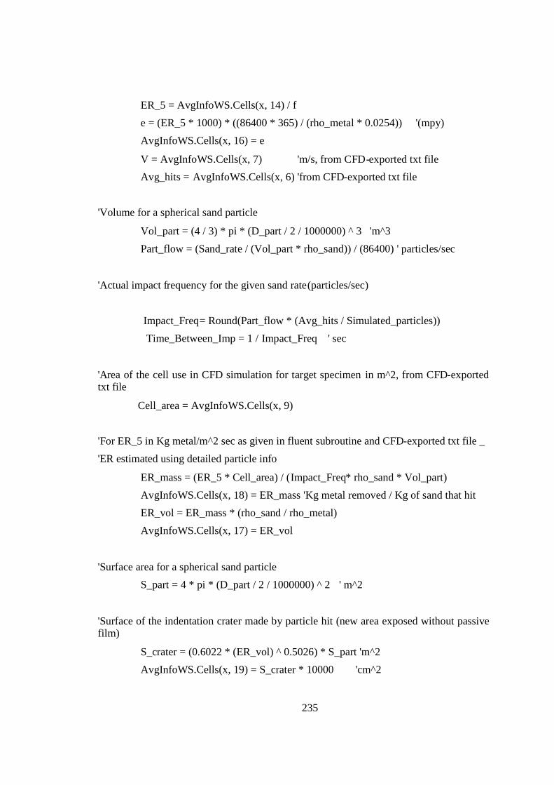
235
ER_5 = AvgInfoWS.Cells(x, 14) / f
e = (ER_5 * 1000) * ((86400 * 365) / (rho_metal * 0.0254)) '(mpy)
AvgInfoWS.Cells(x, 16) = e
V = AvgInfoWS.Cells(x, 7) 'm/s, from CFD-exported txt file
Avg_hits = AvgInfoWS.Cells(x, 6) 'from CFD-exported txt file
'Volume for a spherical sand particle
Vol_part = (4 / 3) * pi * (D_part / 2 / 1000000) ^ 3 'm^3
Part_flow = (Sand_rate / (Vol_part * rho_sand)) / (86400) ' particles/sec
'Actual impact frequency for the given sand rate(particles/sec)
Impact_Freq= Round(Part_flow * (Avg_hits / Simulated_particles))
Time_Between_Imp = 1 / Impact_Freq ' sec
'Area of the cell use in CFD simulation for target specimen in m^2, from CFD-exportedtxt file
Cell_area = AvgInfoWS.Cells(x, 9)
'For ER_5 in Kg metal/m^2 sec as given in fluent subroutine and CFD-exported txt file _
'ER estimated using detailed particle info
ER_mass = (ER_5 * Cell_area) / (Impact_Freq* rho_sand * Vol_part)
AvgInfoWS.Cells(x, 18) = ER_mass 'Kg metal removed / Kg of sand that hit
ER_vol = ER_mass * (rho_sand / rho_metal)
AvgInfoWS.Cells(x, 17) = ER_vol
'Surface area for a spherical sand particle
S_part = 4 * pi * (D_part / 2 / 1000000) ^ 2 ' m^2
'Surface of the indentation crater made by particle hit (new area exposed without passivefilm)
S_crater = (0.6022 * (ER_vol) ^ 0.5026) * S_part 'm^2
AvgInfoWS.Cells(x, 19) = S_crater * 10000 'cm^2

236
'Since I(t)=(Io/(1 + m*Io*t) changed of current with time depends on the product m*Iothis product needs to be adjusted by the new area of the crater
m = m_st * (Stip_st / S_crater)
Io = Io_st * (S_crater / Stip_st)
'Estimation of Average Total current PER CELL of the target specimen on CFDsimullation
T = 0
'initial values
Time(T, 0) = T * Time_Between_Imp ' sec
Time(T, 1) = T * Time_Between_Imp / 3600 'hour
I(T) = Io / (1 + Io * (m / 1000000) * T * Time_Between_Imp)
I_high(T) = I(T)
I_low(T) = 0
I_Avg(T) = (I_high(T) + I_low(T)) / 2
T = 1
Do
If x = 2 Then
Time(T, 0) = T * Time_Between_Imp
Time(T, 1) = T * Time_Between_Imp / 3600
End If
'A quickcalc method based I(T) Instantaneous current for the by the 1st hit
I(T) = Io / (1 + Io * (m / 1000000) * T * Time_Between_Imp)
'I_high(T) tracks the instantaneous response of the highs(peaks) of current caused by thenew hits
I_high(T) = I_high(T - 1) + I(T)
'I_low(T) tracks the instantaneous response of the lows(valleys) of current shown beforenew hits
I_low(T) = I_low(T - 1) + I(T)
'Average between highs and lows
I_Avg(T) = (I_high(T) + I_low(T)) / 2
'Cumulative of the I_Avg as a function of time

237
I_cum(T) = I_cum(T - 1) + I_Avg(T)
'ratio is used as stop criterion
ratio = I(T) / I_high(T)
T = T + 1
No_Particles = T
Loop While ratio >= Stop_Current
'Writing final current on summary sheet
AvgInfoWS.Cells(x, 20) = I_Avg(T - 1)
AvgInfoWS.Cells(x, 21) = I_Avg(T - 1) / (Cell_area * 10000)
'Calculating the Corrosion Component of E-C (CRe-c in mpy)
'Using the E Ratio from detailed particle imp info
AvgInfoWS.Cells(x, 22) = (I_Avg(T - 1)) * (3.27 * EW * 39.37) / _
(rho_metal * AvgInfoWS.Cells(x, 9) * 10000)
'Total E-C in mpy
'Using the E Ratio from detailed particle imp info
AvgInfoWS.Cells(x, 23) = AvgInfoWS.Cells(x, 22) + AvgInfoWS.Cells(x, 16)
w = T
Finally, after the total current per each CFD numerical cell has been estimated by
this code the total current for the whole area specimen is computed by adding up the
current value of each numerical cell. Then, the total current is converted to penetration
rate units by using Faraday’s law and the erosion-corrosion is computed as the sum of the
corrosion component rate Ce-c plus the pure erosion rate E obtained from the average of
the CFD simulation.