testing a correlation coefficientâ€™s significance: using

Psychology Science, Volume 49, 2007 (2), p. 74-87

Testing a correlation coefficient’s significance:Using H0: 0 < is preferable to H0: = 0

KLAUS D. KUBINGER1, DIETER RASCH2 & MARIE ŠIME KOVA3

AbstractThis paper proposes an alternative approach in correlation analysis to significance testing. It argues

that testing the null-hypotheses H0: = 0 versus the H1: > 0 is not an optimal strategy. This is be-cause rejecting the null-hypothesis, as traditionally reported in social science papers – i.e. a significant correlation coefficient (regardless of how many asterisks it is adorned with) – very often has no practi-cal meaning. Confirming a population’s correlation coefficient as being merely unequal to zero does not entail much gain of content information, unless this correlation coefficient is sufficiently large enough; and this in turn means that the correlation explains a relevant amount of variance. The alterna-tive approach, however, tests the composite null-hypothesis H0: 0 < for any 0 < < 1 instead of the simple null-hypothesis H0: = 0. At best, the value of is chosen as the square root of the expected relative proportion of variance which is explained by a linear regression, the latter being the so-called coefficient of determination, 2. The respective test statistic is only asymptotically normally distributed: in this paper a simulation study is used to prove that the factual risk is hardly larger than the nominal risk with regard to the type-I-risk. An SPSS-syntax is given for this test, in order to fill the respective gap in the existing SPSS-menu. Furthermore it is demonstrated, how to calculate the sample size ac-cording to certain demands for precision. By applying the approach given here, no “use of asterisks” would lead a researcher astray – that is to say, would cause him/her to misinterpret the type-I-risk or, even worse, to overestimate the importance of a study because he/she has misjudged the content rele-vance of a given correlation coefficient > 0.

Key words: null-hypotheses testing, correlation coefficient, coefficient of determination, linear de-pendency, sample size determination

1 Klaus D. Kubinger, PhD, Psychological Assessment and Applied Psychometrics, Center of Testing and

Consulting, Faculty of Psychology, University of Vienna, Liebiggasse 5, A-1010 Vienna, Austria, Europe; email: [email protected]

2 Dieter Rasch, DSc, Institute of Statistics University of Agriculture, Vienna, Gregor Mendel Straße 33, A-1180 Vienna, Austria, Europe; email: [email protected]

3 Marie Šime kova, Institute of Animal Science, Praha - Uh ín ves, P átelství 815, 104 01 Praha 114, Czechia, Europe; email: [email protected]


75

1. Introduction

The problem we will discuss in the following, with regard to the correlation coefficient is principally a matter of every other parameter of a distribution. Although many other authors have dealt with the given topic of other parameters in the past – even touching on some aspects of practice in psychology – it was not deliberately taken into consideration for the correlation coefficient, as it will be in this paper. Nevertheless, it is worthwhile to read the discussion of the principle of statistically testing the null-hypothesis in particular by Ballu-erka, Gomez and Hidalgo (2005), where more important references can be found. Additionally see Marks (2006) and the comment by Rasch and Kubinger (2007). Furthermore, the presen-tation of the Neyman-Pearson test theory by Lehmann (1986) is recommended reading.

Although even applied textbooks offer a statistical test for testing the null-hypothesis, that an interesting (product moment) correlation coefficient differs from a given 0 0, this is seldom applied within empirical psychological research. Instead, H0: = 0 is almost always tested against the alternative hypothesis H1: 0. Thereby the convention has been established of calling a correlation coefficient “significant” if this null-hypothesis is rejected, or “not significant” if the null-hypothesis is not rejected. Of course, this meaning of a sig-nificant correlation coefficient is that the correlation coefficient is (absolutely) larger than zero within the given population. Our argument is that merely confirming a population’s correlation coefficient as unequal to zero does not entail much gain of content information, unless this correlation coefficient explains a relevant amount of the variance of the variables. Many psychological researchers – as well as other social science researchers and medical researchers – confound this question of a relevant effect with the level of type-I-risk ( );they practice the so-called “use of asterisks”. We will show that in doing so the importance of a significant correlation coefficient with respect to its content does not increase at all. Consequently, we suggest designing any study, which aims to calculate the (product mo-ment) correlation coefficient, according to pertinent statistical planning conceptualization.

For this we firstly need to call into remembrance the well-known relation of the correla-tion coefficient and the so-called coefficient of determination, in order to suggest a more proper null-hypothesis and a truly relevant effect – that is some distance from the null-hypothesis which is of practical interest. In doing so we, however, have the problem that the resulting statistical test is based on a test statistics of which the distribution is known only asymptotically. Therefore, we did a simulation study investigating the behavior of this test within small sample sizes: the question is whether or not the rate of type-I-errors fits with the nominal value of type-I-risk . Finally we show how to determine the sample size which is needed in order to detect a given relevant effect.

2. The coefficient of determination

There is merely one helpful rule on how to interpret a concrete value of a population cor-relation coefficient , between two linearly dependent random variables x and y. Although it is well-known that this value depends on the angle between both given regression lines (i.e. the line of the regression of x on y and the line of the regression of y on x) this has not led to any measure of practical importance for interpretation. Of course, the sign of is to be un-equivocally interpreted as to whether the variables show a negative or a positive dependency.

K. D. Kubinger, D. Rasch & M. Šime kova76

However, the magnitude of this dependency can best be interpreted by using the coefficientof determination. That results formally in the squared correlation coefficient, 2. This is because the coefficient of determination, , is plausibly defined as the ratio of the variance of one variable, say y, that can be explained by the linear regression on the other variable, say x, to the total variance of y. The following gives proof of = 2.

The basic regression equation is (e an error term; and x and y may be interchange): 0 1y x e = y(x) + e, with the condition that cov , 0x e . Then the coefficient of

determination is 0 1var varvar var

y x xy y

. Let us denote var(e) = 2, 2var xx ,

and 2var yy . Now 2 2 2 2 20 1 1vary xx and because

22

1 4xy

x, with

cov(x,y) = xy the covariance of x and y, we obtain

22

42

2

xyx

x

y.

Analogously the squared sample correlation coefficient r2 can be written as the ratio of the sum of squares, due to linear regression and the total sum of squares of the dependent variable. If multiplied by 100, we have the most informative interpretation of the square of the correlation coefficient, as the percentage of the variance of one of two random variables which can be explained by a linear regression on the other variable – this is true as well for the population as for a sample.

Therefore the interpretation of the linear dependency of two variables must focus on orr concerning the direction, and on 2 or r2 concerning the magnitude. For instance, a correla-tion coefficient with a medium valued numerical result, for instance = .5, does not indicate a medium degree of dependency at all, but merely a weak one, as only 25 % of the variances is mutually explained. Even = .9 does not indicate a very high dependency as only 81 % of the variances is mutually explained. In this case almost a fifth remains unexplained; i.e. a fifth of the variances is determined by other variables or by chance.

A significant correlation coefficient in the sense of > 0, is thus rather arbitrary. Since rejecting H0: = 0 is compatible for instance with = .1 (and of course with even lower values), nothing can be concluded from significance per se; = .1 means a coefficient of determination of .01 and, respectively, only 1 % of the variance or almost no variance is explained by the linear relationship. We do not think that there are many cases within the social sciences where a coefficient of determination of 1 %, or say lower than 10 %, really entails content relevant consequences.

3. The (mis-)”use of asterisks”

The problem is that if we only took a sufficiently large number of observed data pairs into consideration, any arbitrarily small value of r could be significant. We will illustrate this briefly in the following. Given a bivariate normal distribution with = 0 then the sample correlation coefficient calculated from a sample of size n is centrally t-distributed with df = n – 2. Using the formula


77

2

2,2,

2, 2

t n Pr n P

t n P n

(cf. Rasch, Herrendörfer, Bock, Victor & Guiard, 2007) the sample size n can iteratively be calculated with t(n – 2; P) as the P-quantile of the central t-distribution. For instance, a sam-ple size of n = 27 057 always results in a significant correlation coefficient ( = .05) if r is .01 or larger. For r = .1 even a sample size of n = 272 will lead to significance (see for more examples Table 1).

What follows is: “Tell me the number of asterisks or the level of type-I-risk, respec-tively, that you would like and I will tell you the sample size you need to obtain significance even for the case that = .01”. There is however hardly any content relevance for a coeffi-cient of determination < .1, that is < .3162.

Of course, many researchers are aware of this fact. In order to emphasize that a certain sample correlation coefficient r is (absolutely) appropriately high, some researchers “up-grade” (as they think) their significant correlation coefficient by using asterisks: The more asterisks used, the lower the significance level (or the resulting p-value) is – “*” for = .05, “**” for = .01, and “***” for = .001. Such researchers, as well as SPSS in its default setting, imply that a result with many asterisks is of more importance, as the correlation coefficient needs to be higher to result in significance, for instance, in the case of = .01 rather than in the case of = .05. However, as already indicated this is only a question of sample size, not primarily a question of a relevant coefficient of determination, or of a rele-vant effect. Hence, the “use of asterisks” does not exempt the researcher from interpreting the coefficient of determination. Therefore, we recommend always removing the tick (set by default in SPSS) in the box “flag significant correlations”, for then no asterisks and only the p-value are produced.

In general, the “use of asterisks” does not recognize the fact that any a-posteriori deter-mination of an attractive (minimal) type-I-risk – in the sense of a significant result – still always means that the highest a-priori tolerable type-I-risk is accepted. Furthermore, given an actual relevant effect, a p-value that is too low indicates an uneconomic approach in de-signing the experiment or survey because n is too large – the researcher is at fault because an even smaller sample size would have led to significance (cf. Rasch, Kubinger, Schmidtke & Häusler, 2004).

Table 1:Sample sizes n needed to make a given sample correlation coefficient r and coefficient of

determination r2 (in brackets) significant – for three levels of type-I-risk (one-sided alternative hypothesis).

type-I-risk r [r2] .001 .01 .05

.005 [.000025] 381 980 216 476 108 223

.01 [.0001] 95 494 54 119 27 057

.05 [.0025] 3 818 2 165 1 084

.1 [.01] 953 541 272


4. An alternative approach

Rather than suggesting a new test we suggest an alternative approach to formulating the null-hypothesis.

The main problem herewith is that testing the null-hypothesis H0: = 0 against the alter-native hypothesis H1: 0 (or one-sided for instance H1: > 0) does not correspond to any aspect of relevance. However, a state of the art statistical approach would be to design an empirical study, experiment or survey, as follows (cf. for example Rasch & Kubinger, 2006):

fix , the type-I-risk fix , the type-II-risk fix , the minimal effect of relevance.

Now the problem is only one of content: The researcher has to decide in advance which empirical result would entail any consequences of substantial importance. Yet researchers often fail to anticipate such content relevant effects. But at the very latest after the data has been analysed, he/she has to decide on the relevance or irrelevance. In the case of the corre-lation coefficient, obviously few researchers would think of fixing the effect of relevance asdiscussed above, that is = .1, even though it is possible to empirically reject H0: = 0because of an actual = .1. In other words, designing a study as indicated would mean that has to be fixed on a well reflected basis.

However, in doing so it seems proper to discuss the given null-hypothesis as well. As in-dicated above, within the social sciences a .3 and therefore a 2 .09 is seldom of any relevance. Hence, an alternative approach would be to test the pair of hypotheses H0: 0 <

against H1: > instead of H0: = 0 against H1: > 0. That is to use a composite null-hypothesis instead of a simple one. Using this as an example we could for instance define the minimal effect of relevance in terms of the coefficient of determination as follows: All values of < .09 shall belong to that part of the region of parameters according to the given null-hypothesis H0; taking into account the risk that we will accept the null-hypothesis H0

erroneously we may decide that this happens only with a probability of .2 (the type-II-risk )if > .25. Consequently, the minimal effect of relevance amounts to ( = 2) = .25 – .09 = .16 and ( ) = .5 – .3 = .2. Having decided on this, we can now calculate the sample size needed.

There is only a technical statistical problem when using the null-hypothesis H0: 0 < . While an exact test for 0 exists which is based on a test-statistic with a known distri-

bution, this is not the case for 0 . The respective test-statistic u is only asymptotically normally distributed (see R.A. Fisher’s theorem in the Appendix). The test needs to trans-

form as well as r as follows: 1 1ln2 1

and 1 1ln2 1

rzr

. Then 3nu z is

the respective asymptotically standard normally distributed test statistic. H0 will be rejected if 1u u , the 1 -quantile of the one-sided standard normal distribution.

Unfortunately the SPSS menu does not offer this test. Therefore, we have provided the SPSS syntax for the calculation of u in Figure 3 of the Appendix to make this test available for every SPSS user.


79

In the hardly relevant case of a two-sided alternative hypothesis, that is to

test 0 :H against H1:or

, we would only have to reject H0 if

12

u u .

5. Properties of the test

As already indicated the distribution of the test given in chapter 4 is only asymptotically known. In order to gain knowledge on the quality of approximation of the actual type-I-risk by using this distribution for small sample sizes, we carried out a simulation study. That disclosed that even for a relatively small n the asymptotic test has a monotonous increasing power function, with the maximum of the type-I-risk at (cf. Fig. 1). The simulation was done for = .05, = .3 and n = 10, 20, ..., 80 by generating bivariate normal random vari-ables with given correlation coefficients . The determination of the power function was done with arguments varying in steps of .01 within the interval (0, 1). The result is an “empirical” power function which is compared with the theoretical power function of a test, based on an exact standard normal distributed test statistic u*. We found that the theoretical power is less than the empirical power (see again Fig. 1 for n = 10, 20, ..., 60 and see for n =10, 20, ..., 1500 in Tab. 2 the empirical power function especially for = = .3, which there-fore meets the actual type-I-risk). Even for the relatively small sample size n = 40 the theo-retical power function comes close to the empirical one, so that both cannot be visually dis-tinguished.

Figure 1:The power function of the test

given in chapter 4. The em-pirical power function is given in black, the theoretical one in

grey.4

pow

er

0.0

0.2

0.4

0.6

0.8

1.0

0.0 0.1 0.2 0.3 0.4 0.5 0.6 0.7 0.8 0.9 1.0

102030405060

4 The estimation of the actual type-I-risk is based on 200 000 simulations.


Table 2:Actual values of the type-I-risk, act, of the asymptotic test for = .3 depending on the sample

size – the standard deviation included.5

Sample size act Standard deviation of act

10 .0537 .00059 20 .0531 .00053 30 .0525 .00054 40 .0524 .00046 50 .0520 .00046 60 .0521 .00053 70 .0519 .00039 80 .0515 .00051 100 .0514 .00032 150 .0514 .00056 200 .0511 .00050 300 .0506 .00056 400 .0507 .00039 500 .0506 .00046 750 .0506 .00043

1000 .0505 .00036 1500 .0503 .00061

The higher power of the asymptotic test compared with the theoretical power means that in the region of the null-hypothesis the actual type-I-risk, act, exceeds the nominal type-I-risk, nom = .05. In order to get an impression of how the given results depend on nom and ,Table 3 gives act for n = 50.

Table 3:Actual values of the type-I-risk, act, of the asymptotic test for three different and three different

nom (n = 50) – in brackets the standard deviation of act.6

nom .01 .05 .10

0 .0103 (.00058)

.0503(.00150)

.1004(.00217)

.3 .0117 (.00083)

.0520(.00046)

.1025(.00303)

.7 .0113 (.00078)

.0545(.00192)

.1074(.00309)

5 The estimation of the actual type-I-risk is based on 2 000 000 simulations; the respective standard deviation

is based on 10 times 200 000 simulations. 6 The estimation of the actual type-I-risk is based on 200 000 simulations; the respective standard deviation is

based on 10 times 20 000 simulations.


81

The result is that there is always a higher actual value of the type-I-risk of less than 10 % of the nominal type-I-risk. For = .3, we therefore suggest that if one wants to be on the safe side with this asymptotic test then nom = .0465 should be used instead of .05, because this would lead to an act ~.05. This means we reject H0 if u > u(0.9535) = 1.6798.

6. Sample size determination

When designing an empirical study properly, the researcher is of course in a position to calculate the particular sample size that guarantees a certain type-I- and type-II-risk for a given effect size which is fixed in advance. We will illustrate this in the following by using a numerical example, with the programme package CADEMO7.

As already discussed we will use = .3 as this gives a coefficient of determination of nearly 10 %. Within psychology, for instance, many variables correlate with each other around .3 although they are essentially interpreted as being independent – compare several personality questionnaire scales correlated with several intelligence subtests. Then we will use a type-I-risk = .05 and a type-II-risk = .2. Of course, such risks have to be consid-ered as we do not want to investigate the whole population but only n members sampled randomly. Hence, we, for instance, fix = .2 because then an existing > + = .5 will not be overlooked with a probability of at least 1- = .8. This means a coefficient of determina-tion of 2 > .25 will only lead to accepting the null-hypothesis (H0: 0 < .3) with the prob-ability of .2 at the most. Of course, a suitable alternative would be = .4 as then at least almost half of the variance would be explained.

We calculate the respective minimal sample size n by using CADEMO and apply the

One sample problem Correlation Coefficient Test …

which leads to Figure 4 (in the Appendix), where we confirm as already decided: alpha=0.05 and beta= 0.20; and we have chosen r0 = 0.3 (= ) and lastly clicked on One-sidedr>r0+d and inserted d = 0.2 (= ). After pressing OK the result of n = 111 is calculated as shown in Figure 5 (in the Appendix).

To illustrate the advantage of this approach, we will give an empirical example8. The question is, whether or not a specific new intelligence subtest (Verbal Reasoning Test) corre-lates with an other certain pertinent intelligence subtest (Applied Computing). In answering this question, all parameters are chosen as indicated. In fact, n = 111 persons were sampled. Figure 2 gives the listings from SPSS. The correlation coefficient is obviously significant in the sense that the null-hypothesis H0: = 0 is rejected. The researcher is persuaded that his/her type-I-risk is in accordance with .01, although it is only chosen when the result of the analysis is already known – this applies even more so if the tick in the box: “flag significant correlations” has not been removed, and the correlation coefficient is marked by two aster-isks. Besides he/she is persuaded to believe in an impressive effect because of significance

7 a demonstration version of CADEMO which serves for this purpose is available at www.biomath.de (details

for using CADEMO see at Rasch & Kubinger, 2006). 8 We thank Karin Placek for making her data available to us (see for details Placek, 2006).


even at this very low significance level, although may not differ very much from zero. In the best of the worst case scenario, the researcher would nevertheless interpret the estimated coefficient of determination of .22 (.4732) as about only a fifth of explained variance.

Correlationen

AppliedComputing Verbal Reasoning Test

Pearson Correlation 1 ,473Sig. (2-tailed) ,000

Applied Computing

N 111 111Pearson Correlation ,473 1Sig. (2-tailed) ,000

Verbal Reasoning Test

N 111 111

Figure 2:SPSS listing of the Pearson correlation coefficient

In comparison, applying the alternative approach, using the SPSS syntax given in Figure 3, leads to a p = .0168, which is less than = .05. Now, as we have designed the study and calculated the appropriate sample size, we reject H0: 0 < .3 and accept H1: > .3. We are completely confident that each and every researcher will profit far more from this conclu-sion, than from the mere information that the correlation coefficient is very probably not zero.

7. Discussion

A naïve researcher who is interested in a correlation coefficient, the square of which shall explain at least 25% of the total variance, may have the idea of testing H0: 0 < .5versus H1: > .5 instead of using the approach suggested above. However, in doing this he/she is not taking the type-II-risk into consideration. This means, for instance, for a sample size of n = 20 that any sample correlation coefficient r between .5 and .7422 leads, with an unacceptably large probability of at least = .5, to incorrectly accepting the null-hypothesis – coin tossing would give the same rate of hits. Only the calculation of n accord-ing to a predetermined , , and guarantees a decision for one of the two hypotheses at known and generally acceptable risks.

An eager researcher’s question still remains to be discussed: Why should he/she not test H0: = 0 with a = .5 for the sample size determination, instead of testing H0: 0 < .3 with = .2 as proposed here? As a matter of fact, having decided for = .05 and = .2 only the sample size n = 24, instead of n = 111, would be needed. The answer is that in both cases


83

of planning the study we aim for an n that allows for a factually given > .5 to be discov-ered by the test with at least the probability 1- . That is, if the null-hypothesis is accepted then we have to be aware of the fact that it is incorrectly accepted, in the long run, in up to 20 % of such studies – given > .5 indeed. If, on the other hand, the null-hypothesis is re-jected, this means that in the one case the data is compatible with > 0, but in the other case it is more concretely only compatible with > .3.

Finally, we have to point out that the description of “significant” for the approach given here should rather not be used due to the danger of misunderstandings. If indeed the null-hypothesis is rejected, then it is better to interpret it as follows: “the correlation coefficient is significantly greater than ”.

Last but not least: In applying this approach no “use of asterisks” would lead a researcher astray, i.e. cause him/her to misinterpret the type-I-risk or even worse to overestimate the importance of a study as he/she misjudges the content relevance of a correlation coefficient > 0.

8. Final recommendations

Summarising the suggested approach we recommend the following: A coefficient of determination less than = 2 = .09 and a correlation coefficient less than = .3 is of no considerable content relevance. Therefore, the null-hypothesis should be formulated as: H0: 0 < = .3, and the alter-native hypothesis as H1: > .3. The type-I-risk may be fixed at = .05 and the type-II-risk at = 0.2 for all cases of >

+ = .5. Consequently a sample size of n = 111 is needed. Testing the null-hypothesis can then be performed by the SPSS syntax command as it is given in Figure 3 in the Ap-pendix .

For a few other values of , , , and the minimal sample sizes, according to CA-DEMO, are given in Table 4 in the Appendix.

Acknowledgement

This paper was partially supported by the research grant MZE 000 2701403 of the Minis-try of Agriculture of the Czech Republic.

References

Balluerka, N., Gomez, J. & Hidalgo, D. (2005). The controversy over null hypothesis signifi-cance testing revisited. Methodology, 1, 55-70.

Fisher, R.A. (1921). On the “probable error” of a coefficient of correlation deduced from a small sample. Metron, 1, 3-32.

Rasch, D. & Kubinger, K.D. (2007, in print). Kommentar: „Das will aber in die Köpfe der Sta-tistik-Nutzer partout nicht hinein“ – ein ergänzender Kommentar zu Marx (2006): Das Null-


Ritual [Commentary: „You just can’t get it into statistics users’ heads“ – a supplementary commentary to Marx (2006): Testing against zero]. Psychologische Rundschau.

Lehmann, E. L. (1986). Testing statistical hypotheses. (2nd ed.). New York: Wiley. Marx, W. (2006). Kommentar: Das Null-Ritual und einer seiner Bewunderer [Commentary: The

ritual of testing against the effect of zero]. Psychologische Rundschau, 57, 256-258.Placek, K. (2006). Dimensionalitätserweiterung des AID 2 um eine Reasoning-Komponente: Der

Verwandtschaften-Reasoning-Test [Expansion of the intelligence test battery AID 2 by a rea-soning test: The Relationship Reasoning Test]. Master Thesis, Vienna: Univ. of Vienna.

Rasch, D., Herrendörfer, G., Bock, J., Victor, N., & Guiard, V. (2007). Verfahrensbibliothek Versuchsplanung und -auswertung [Library of Statistical Procedures: Design and Planning]. (2nd ed.). München: Oldenbourg.

Rasch, D. & Kubinger, K.D. (2006). Statistik für das Psychologiestudium – Mit Softwareunter-stützung zur Planung und Auswertung von Untersuchungen sowie zu sequentiellen Verfahren [Statistics for the study of psychology – with software support for the planning of studies and sequential procedures]. Munich: Spektrum.

Rasch, D., Kubinger, K.D., Schmidtke, J. & Häusler, J. (2004). The Misuse of Asterisks in Hy-pothesis Testing. Psychology Science, 46, 227-242.


85

Appendix

Theorem (R.A. Fisher, 1921)In the sequel 2;AN means asymptotically (i.e. for n ) normally distributed.

If

1 1

2 2

n n

x yx y

x y is a random sample from a two-dimensional normal distribution with corre-

lation coefficient then 1

2 2

1 1

n

i ii

n n

i ii i

x x y yr

x x y y is a biased estimator of and

AN(

221;

n).

It is known that the asymptotic is very slow. The following Corollary gives a slightly better asymptotic:

1 1ln2 1

rzr

is AN 1 1 1ln ;2 1 2 1 3n n

.

Additional Figures and Tables

Figure 3:SPSS syntax for testing H0:


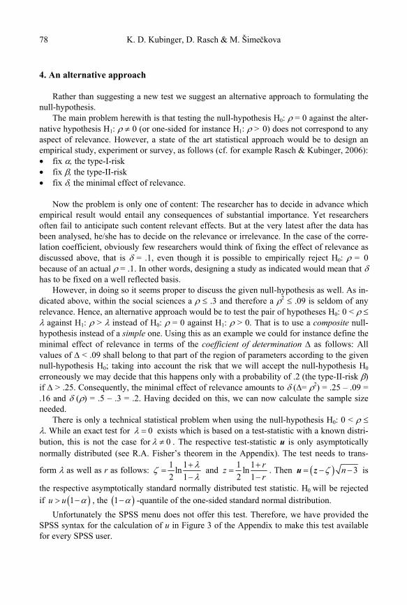
Figure 4:Input for CADEMO for the calculation of n in order to test the (product moment) correlation coefficient according to given type-I- and type-II-risks and , respectively, and the effect of

content relevance (in CADEMO we have = d and = r0).

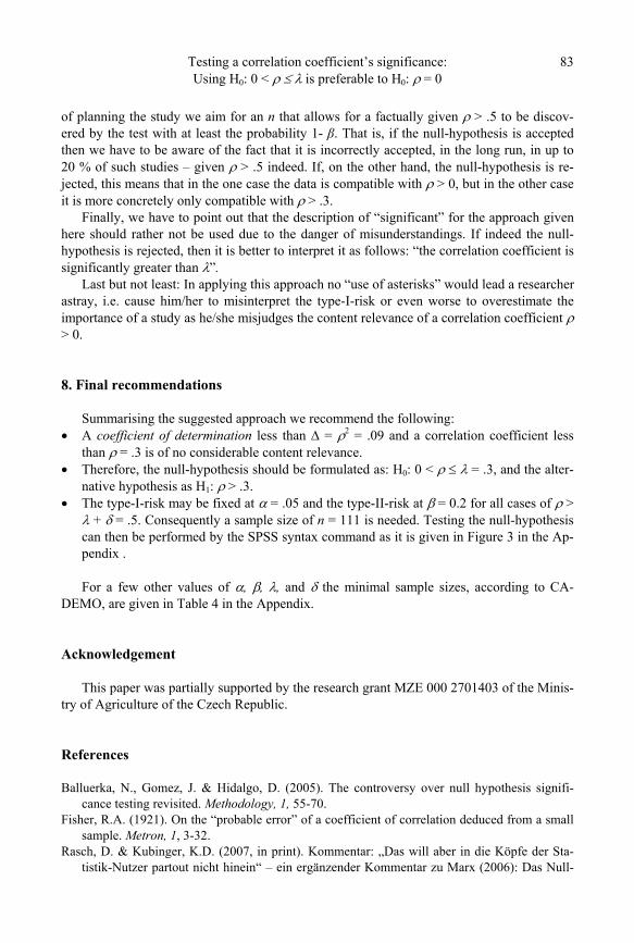
Figure 5:Result from CADEMO for the calculation of n in order to test the (product moment) correlation

coefficient according to given type-I- and type-II-risks and the effect of content relevance (H0, 0 < , > 0; and a one-sided alternative hypothesis).


87

Table 4:Minimal sample sizes needed for some selected values of , , , and

= .2 = .3 = .4

= .2 = .4 = .2 = .4 = .2 = .4.05 327 69 278 54 221 38 .01.1 270 58 230 45 183 32 .05 225 48 192 38 153 27 .1 179 39 152 31 121 22 .05.2 130 29 111 23 89 17

J. Frommer, D. L. Rennie (Eds.)

Qualitative Psychotherapy Research - Methods and Methodology -

Qualitative psychotherapy research has a long past but a short history. In this informa-tive volume of contributions by leading European and Anglo-American researchers, with the former focusing on the psychoanalytic interview as an unrecognized early and powerful form of qualitative research, and the latter on approaches such as grounded theory and types of discourse analysis, the volume both covers and extends the range of qualitative therapy research inquiry. Throughout, attention is paid to me-thodology as well as methods, in the interest of defining the principles and standards governing this approach. With most of the contributors being psychotherapists themselves, their writings are deeply contextualized in therapeutic practice. This book thus holds interest for re-searchers and practitioners alike, especially in terms of the ways it offers of closing the well-known gap between them. 2nd Edittion 2006, 208 pages, 24,- Euro ISBN 978-3-935357-74-6 (Europe) ISBN 1-59326-031-8 (USA)

PABST SCIENCE PUBLISHERS

Eichengrund 28, D-49525 Lengerich, Tel. ++ 49 (0) 5484-308, Fax ++ 49 (0) 5484-550 [email protected], www.psychologie-aktuell.com, www.pabst-publishers.de

testing a correlation coefficientâ€™s significance: using

Documents