1

Test Methods for Assessing Long-term Properties of Corrugated HDPE Pipes (Part I- Long-term Modulus)

1. INTRODUCTION

The full specification of 100-year corrugated HDPE pipes is pending on three additional tests which

are creep rupture of the pipe line (FM-575), long-term tensile strength (FM-576), and long-term modulus

(FM-577). Based on the results of the previous project and recently changes in the pipe resins,

modifications are required for these three test methods in order to determine the long-term mechanical

properties within reasonable testing duration. In this report, the modified test method to determine long-

term modulus is presented by performing laboratory tests to verify the test procedures.

2. BACKGROUND The current design parameters for corrugated HDPE pipe specified by AASHTO Section 17 are

shown in Table 1. The initial (short term) tensile strength and flexural modulus of elasticity are taken

from the material specification ASTM D3350 based on a cell class of 435400C. For the long term

property values, AASHTO Section 17 states that “these values are derived from hydrostatic design bases

(HDB) and indicate a minimum 50-year life expectancy under continuous application of tensile stress”.

Thus, the 50-year modulus values listed in Table 1 were obtained under a creep mode.

Table 1 – Mechanical Properties for Design HDPE Pipes (NCHRP 631)

Material Tensile Values (psi) Modulus Values (psi)

Initial Long-term Initial Long-term

50-yr 75-yr 100-yr 50-yr Creep mode

75-yr Relaxation

mode

100-yr Relaxation

mode Corrugated Pipe AASHTO M294

3000 900 NA NA 110,000 22,000 21,000 20,000

Profile Pipe ASTM F894

2600 NA NA NA 80,000 20,000 19,000 18,000

Note: NA = not available

For modulus beyond 50-year service life, values for 75-year and 100-year of corrugated and profile

HDPE pipes were proposed in the recently published NCHRP Report 631 (McGrath et al., 2008), and

these values are also included in Table 1. These two proposed modulus values were estimated based on

published literature. NCHRP Report 631 referenced Janson 1985(a) and Chua (1986) in which the Power

Law (Eq. (1)) were used to predict the relaxation modulus of HDPE. Using parameters given by Janson

2

(1985a) and Chua (1986), the predicted 100-year relaxation modulus using Eq. (1) was found to be

18,300 psi and 18,000 psi, respectively.

E(t) = E∞ + (E1 - E∞)*t-m (1)

Where: E(t) is the relaxation modulus at a given time, E∞ is the relaxation modulus at very long time; E1 is the modulus at one unit of time, and m is the rate of decrease of modulus, and t is time.

Additional viscoelastic and viscoplastic models were also presented in NCHRP Report 631 which can be

used to predict the long-term properties of HDPE pipe. However, the verification of these models was

based on creep or stress relaxation less than 10,000 hours at room temperature. Therefore there would be

certain degrees of uncertainty of such prediction.

In this study, the long-term modulus of corrugated HDPE pipe junction was evaluated the stepped

isothermal method (SIM), which is a relatively new acceleration method to predict the creep behavior of

polymeric materials. The results of SIM were validated by the traditional accelerated creep test, time-

temperature superposition (TTS). Recommendation was proposed for assessing long-term creep modulus

of corrugated HDPE pipe together with standard test method.

3. FLEXURAL MODULUS OF PIPE

3.1. Initial (short-term) Modulus

The initial modulus values listed in Table 1 were obtained from test specimens taken from

compression molded plaques prepared from pristine HDPE resins. The effects of the pipe manufacturing

process and carbon black additives on the properties are not considered. In addition, the modulus is

determined by a flexural test (ASTM D 790) at 2% strain, i.e. 2% secant modulus, at standard laboratory

ambient temperature.

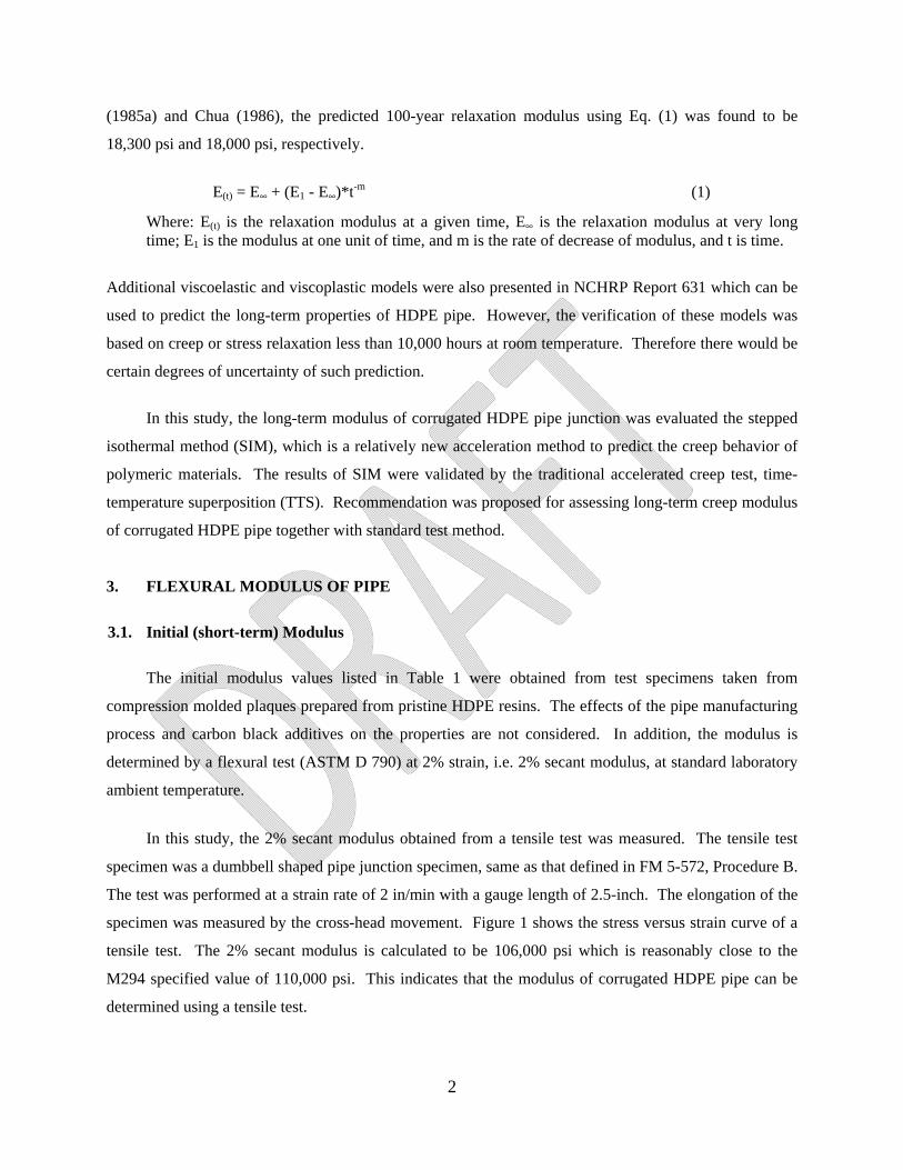
In this study, the 2% secant modulus obtained from a tensile test was measured. The tensile test

specimen was a dumbbell shaped pipe junction specimen, same as that defined in FM 5-572, Procedure B.

The test was performed at a strain rate of 2 in/min with a gauge length of 2.5-inch. The elongation of the

specimen was measured by the cross-head movement. Figure 1 shows the stress versus strain curve of a

tensile test. The 2% secant modulus is calculated to be 106,000 psi which is reasonably close to the

M294 specified value of 110,000 psi. This indicates that the modulus of corrugated HDPE pipe can be

determined using a tensile test.

3

3.2. Long-term Modulus

3.2.1. Conventional test

Ideally, the long-term modulus should be determined from either creep or stress relaxation tests for

a minimum testing time of 10,000 hours (i.e., ~ 1.14 years) at the site specific temperature. However,

even with test duration of 10,000 hours, there would be uncertainty using such test data to predict the

long-term modulus for service life of 50 to 100 years at the same temperature, since the extrapolation is

well beyond two-log cycles. Although, various theoretical models (viscoelastic, viscoplastic, constitutive

models, etc.) have been developed to predict the long-term behavior of the polymer, the verification of

these models is limited to test data up to 10,000 hours (Chua and Lytton, 1989; Zhang and Moore,

1997(a), (b); Drozdov and Kalamkarov, 1996; Lai and Bakker, 1995).

3.2.2. Time-temperature superposition method

Time-temperature superposition (TTS) is a widely used acceleration test to evaluate the viscoelastic

behavior of polymeric materials. In this method, the time factor can be reduced by elevated temperature

(Nielsen, 1974; Ferry, 1980; Moore and Kline, 1984; Painter and Coleman, 1997). Creep or stress

relaxation curves obtained at elevated temperatures can then be shifted along the time scale to generate a

master creep curve for use at a lower reference temperature. The common test duration at each

temperature step of TTS is 1,000 hours. The maximum elevated test temperature and the number of

temperature steps would depend on the desired time duration of the master curve. In this test, a new

Figure 1 – Tensile stress-strain curve using pipe junction specimen

0

500

1000

1500

2000

2500

3000

3500

4000

0 10 20 30 40 50 60

Stre

ss (p

si)

Elongation (%)

4

specimen is used for each temperature step; thus, variability among specimens can induce errors in the

test result.

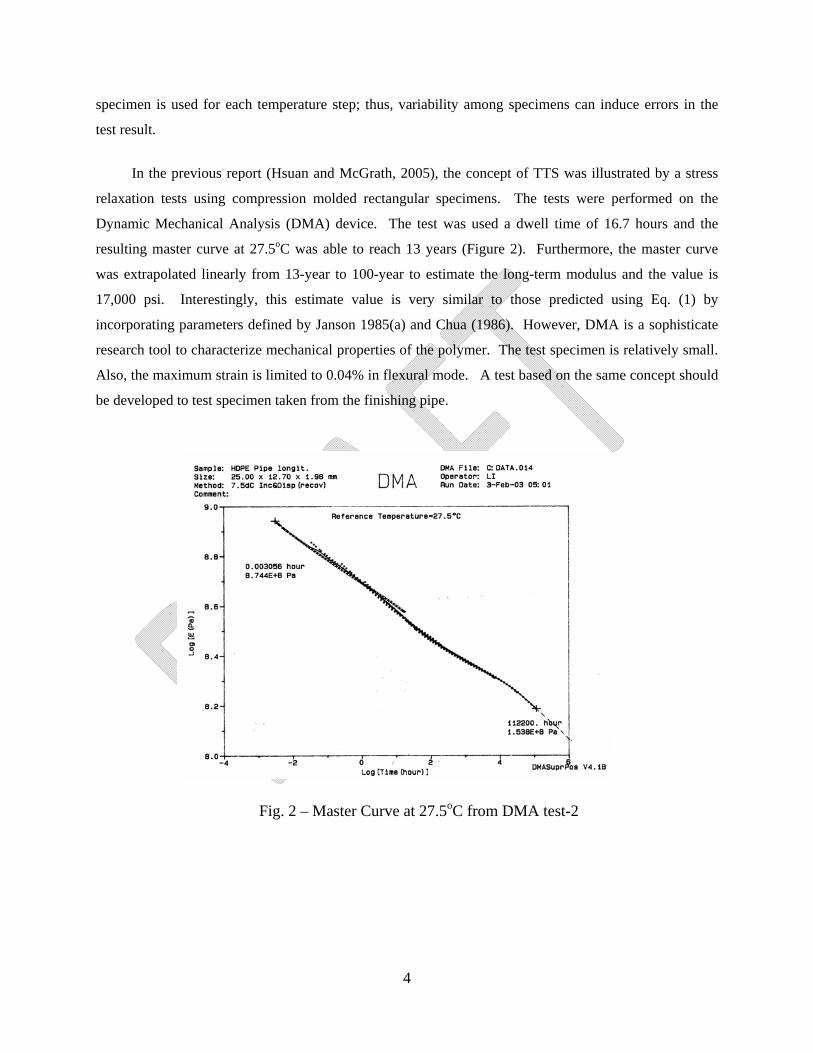
In the previous report (Hsuan and McGrath, 2005), the concept of TTS was illustrated by a stress

relaxation tests using compression molded rectangular specimens. The tests were performed on the

Dynamic Mechanical Analysis (DMA) device. The test was used a dwell time of 16.7 hours and the

resulting master curve at 27.5oC was able to reach 13 years (Figure 2). Furthermore, the master curve

was extrapolated linearly from 13-year to 100-year to estimate the long-term modulus and the value is

17,000 psi. Interestingly, this estimate value is very similar to those predicted using Eq. (1) by

incorporating parameters defined by Janson 1985(a) and Chua (1986). However, DMA is a sophisticate

research tool to characterize mechanical properties of the polymer. The test specimen is relatively small.

Also, the maximum strain is limited to 0.04% in flexural mode. A test based on the same concept should

be developed to test specimen taken from the finishing pipe.

Fig. 2 – Master Curve at 27.5oC from DMA test-2

5

3.2.3. Stepped isothermal method

Stepped Isothermal Method (SIM) is a relatively new method that was developed in the 1990’s to

evaluate polymeric reinforcing materials, known as geogrid (Thornton et al., 1998(a) and (b); Greenwood

and Voskamp, 2000). The methodology was first used by Sherby and Dorn (1958) to evaluate the creep

property of polymethyl-methacrylate (PMMA). The method combines both TTS and Boltzmann

superposition. In SIM, a single specimen is exposed to a series of temperature steps under a constant

applied load to generate a sequence of creep curves from which the master creep curve is formed. The

advantage of SIM is further shortening the testing time and avoiding material variability in comparison to

TTS.

4. TEST MATERIALS

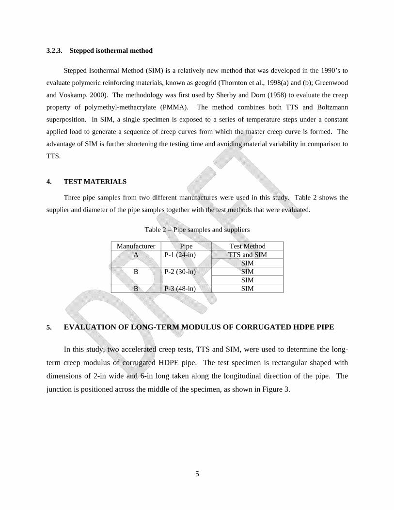
Three pipe samples from two different manufactures were used in this study. Table 2 shows the

supplier and diameter of the pipe samples together with the test methods that were evaluated.

Table 2 – Pipe samples and suppliers

5. EVALUATION OF LONG-TERM MODULUS OF CORRUGATED HDPE PIPE

In this study, two accelerated creep tests, TTS and SIM, were used to determine the long-

term creep modulus of corrugated HDPE pipe. The test specimen is rectangular shaped with

dimensions of 2-in wide and 6-in long taken along the longitudinal direction of the pipe. The

junction is positioned across the middle of the specimen, as shown in Figure 3.

Manufacturer Pipe Test Method A P-1 (24-in) TTS and SIM

SIM B P-2 (30-in) SIM

SIM B P-3 (48-in) SIM

6

Figure 3 – Pipe junction specimen for the creep test

5.1. TTS Experiment and Results Figure 4 shows the test set up for the TTS test. The load was applied to the specimens using the

cantilever dead weight. The deformation of the specimens was measured with a dial gauge. The test

specimens were mounted inside of an environmental chamber, which was fabricated using extruded

polystyrene foam panel with thickness of 25.4 mm. The chamber was 800 mm (W) × 400 mm (H) × 280

mm (L). A flat heater and a thermocouple connected to a temperature controller were placed inside the

chamber. A fan was positioned adjacent to the heater to achieve temperature uniformity. The accuracy of

temperature in the chamber was ± 0.5oC.

Figure 4 – Test set-up for TTS

6 in

2 +/- 0.1 inLongitudinal

Circumferential

ValleyLiner

Machine Direction

Corrugationremoved

7

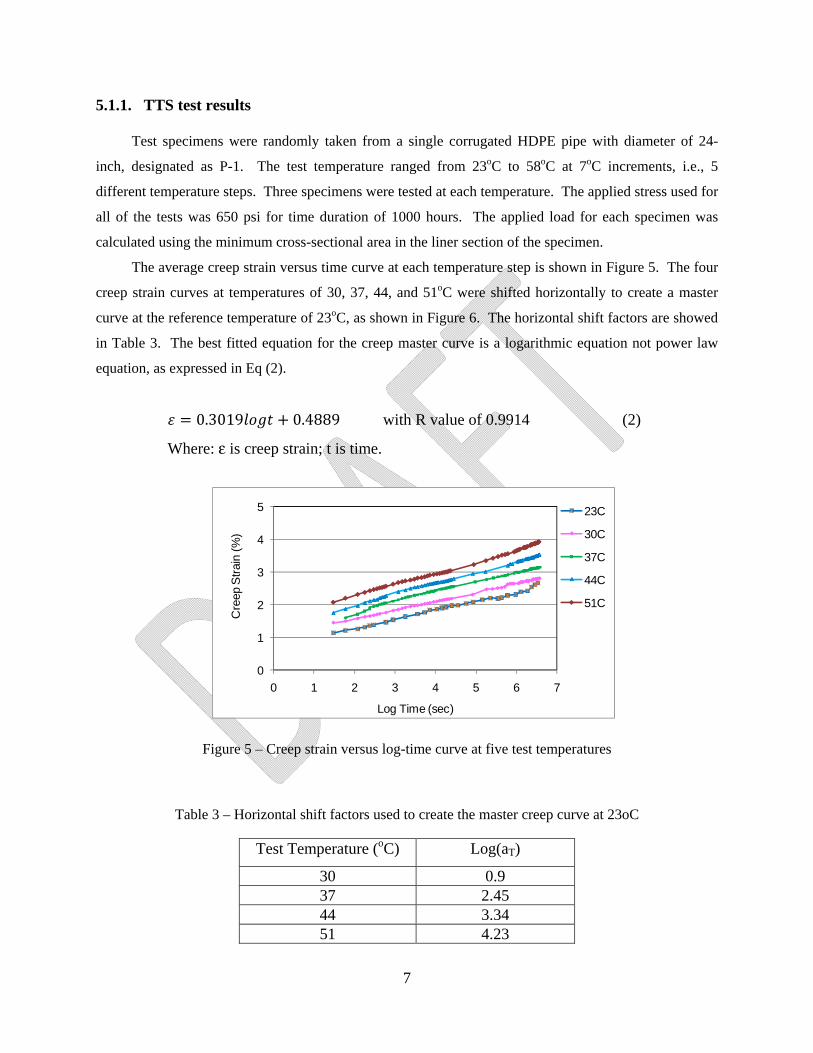
5.1.1. TTS test results Test specimens were randomly taken from a single corrugated HDPE pipe with diameter of 24-

inch, designated as P-1. The test temperature ranged from 23oC to 58oC at 7oC increments, i.e., 5

different temperature steps. Three specimens were tested at each temperature. The applied stress used for

all of the tests was 650 psi for time duration of 1000 hours. The applied load for each specimen was

calculated using the minimum cross-sectional area in the liner section of the specimen.

The average creep strain versus time curve at each temperature step is shown in Figure 5. The four

creep strain curves at temperatures of 30, 37, 44, and 51oC were shifted horizontally to create a master

curve at the reference temperature of 23oC, as shown in Figure 6. The horizontal shift factors are showed

in Table 3. The best fitted equation for the creep master curve is a logarithmic equation not power law

equation, as expressed in Eq (2).

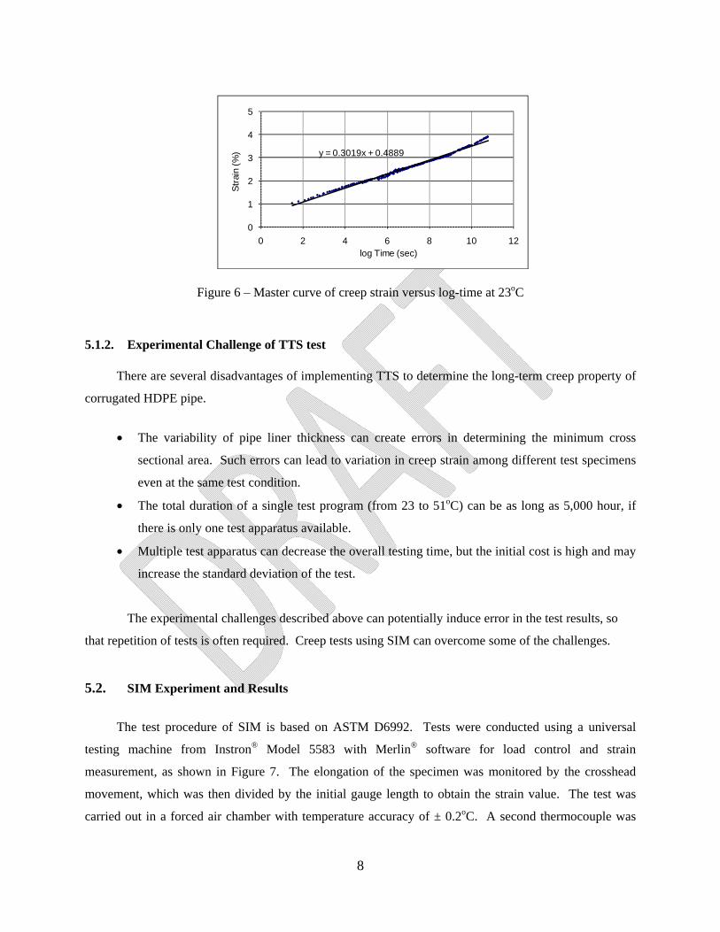
0.3019 0.4889 with R value of 0.9914 (2)

Where: ε is creep strain; t is time.

Figure 5 – Creep strain versus log-time curve at five test temperatures

Table 3 – Horizontal shift factors used to create the master creep curve at 23oC

Test Temperature (oC) Log(aT)

30 0.9 37 2.45 44 3.34 51 4.23

0

1

2

3

4

5

0 1 2 3 4 5 6 7

Cre

ep S

trai

n (%

)

Log Time (sec)

23C

30C

37C

44C

51C

8

Figure 6 – Master curve of creep strain versus log-time at 23oC

5.1.2. Experimental Challenge of TTS test There are several disadvantages of implementing TTS to determine the long-term creep property of

corrugated HDPE pipe.

• The variability of pipe liner thickness can create errors in determining the minimum cross

sectional area. Such errors can lead to variation in creep strain among different test specimens

even at the same test condition.

• The total duration of a single test program (from 23 to 51oC) can be as long as 5,000 hour, if

there is only one test apparatus available.

• Multiple test apparatus can decrease the overall testing time, but the initial cost is high and may

increase the standard deviation of the test.

The experimental challenges described above can potentially induce error in the test results, so

that repetition of tests is often required. Creep tests using SIM can overcome some of the challenges.

5.2. SIM Experiment and Results

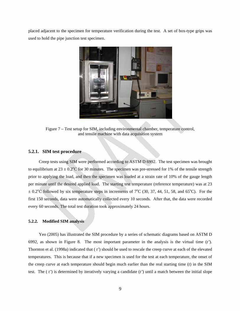
The test procedure of SIM is based on ASTM D6992. Tests were conducted using a universal

testing machine from Instron® Model 5583 with Merlin® software for load control and strain

measurement, as shown in Figure 7. The elongation of the specimen was monitored by the crosshead

movement, which was then divided by the initial gauge length to obtain the strain value. The test was

carried out in a forced air chamber with temperature accuracy of ± 0.2oC. A second thermocouple was

y = 0.3019x + 0.4889

0

1

2

3

4

5

0 2 4 6 8 10 12S

trai

n (

%)

log Time (sec)

9

placed adjacent to the specimen for temperature verification during the test. A set of box-type grips was

used to hold the pipe junction test specimen.

Figure 7 – Test setup for SIM, including environmental chamber, temperature control, and tensile machine with data acquisition system

5.2.1. SIM test procedure

Creep tests using SIM were performed according to ASTM D 6992. The test specimen was brought

to equilibrium at 23 ± 0.2oC for 30 minutes. The specimen was pre-stressed for 1% of the tensile strength

prior to applying the load, and then the specimen was loaded at a strain rate of 10% of the gauge length

per minute until the desired applied load. The starting test temperature (reference temperature) was at 23

± 0.2oC followed by six temperature steps in increments of 7oC (30, 37, 44, 51, 58, and 65oC). For the

first 150 seconds, data were automatically collected every 10 seconds. After that, the data were recorded

every 60 seconds. The total test duration took approximately 24 hours.

5.2.2. Modified SIM analysis

Yeo (2005) has illustrated the SIM procedure by a series of schematic diagrams based on ASTM D

6992, as shown in Figure 8. The most important parameter in the analysis is the virtual time (t’).

Thornton et al. (1998a) indicated that ( t’) should be used to rescale the creep curve at each of the elevated

temperatures. This is because that if a new specimen is used for the test at each temperature, the onset of

the creep curve at each temperature should begin much earlier than the real starting time (t) in the SIM

test. The ( t’) is determined by iteratively varying a candidate (t’) until a match between the initial slope

10

of the strain curve to the end slope of the previous strain curve in a strain versus log-time plot is obtained

(Allen, 2005).

However, Yeo and Hsuan (2005) found that the analytical procedure using (t’) is not applicable for

HDPE geogrid due to the high thermal expansion and low thermal conductivity properties. The HDPE

geogrid require a much longer time to reach equilibrium than the polyester geogrid at each elevated

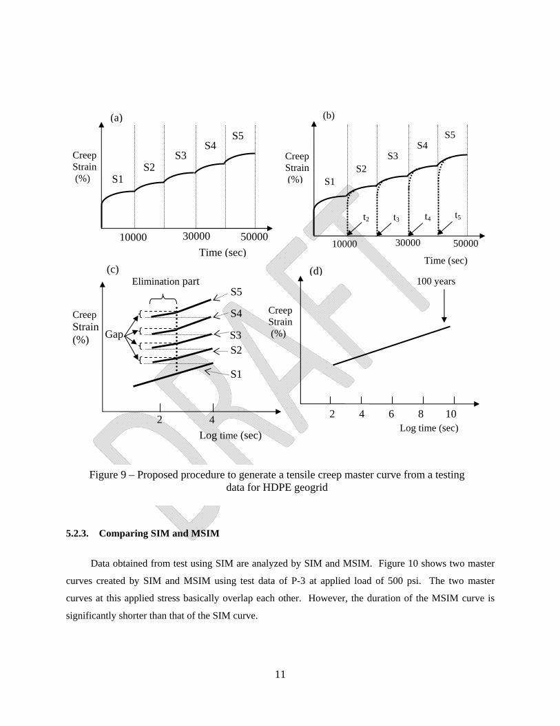
temperature step. Thus a modified procedure was proposed to analyze the data from SIM. The modified

procedure (called the MSIM) does not use (t’) in the analysis, as illustrated in Figure 9. The initial non-

equilibrium portion of the creep curve was removed and the remaining creep curves are shifted

horizontally and vertically to create the master curve. Thus, the resulting master curve is much shorter

than that obtained from the SIM procedure using the same number of temperature steps. In this study,

both analyses, SIM and MSIM, are evaluated.

Creep Strain (%)

Time (sec) t2 t2’

t3 t4 t5

t3’ t4’ t5’

(b)

Log time (sec)

S2S3S4S5

(c)

S1

4 2

Creep Strain (%)

Creep strain (%)

100 years

Log time (hr)

-2 0 2 4 6

(d)

Figure 8 – Procedure to generate a tensile creep master curve from a testing data for HDPE geogrid by ASTM

Creep Strain (%)

Time (sec)

S1 S2\

S3 S4

S5

(a)

10000 30000 50000

11

5.2.3. Comparing SIM and MSIM

Data obtained from test using SIM are analyzed by SIM and MSIM. Figure 10 shows two master

curves created by SIM and MSIM using test data of P-3 at applied load of 500 psi. The two master

curves at this applied stress basically overlap each other. However, the duration of the MSIM curve is

significantly shorter than that of the SIM curve.

Creep Strain (%)

Time (sec)

S1 S2

S3 S4

S5

(a)

10000 30000 50000

Creep Strain (%)

100 years

Log time (sec) 2 4 6 8 10

(d)

Figure 9 – Proposed procedure to generate a tensile creep master curve from a testing data for HDPE geogrid

Creep Strain (%)

Time (sec)

S1 S2

S3 S4

S5

(b)

10000 30000 50000

t2 t3 t4 t5

Log time (sec)

S2 S3

S4

S5

(c)

S1

Elimination part

4 2

Creep Strain (%) Gap

12

If SIM is used to analyze the test data, the temperature steps can be shortened from 6 to 5

increments to reach the 100 year creep strain, and the entire test will take approximately 15 hours. On the

other hand, temperature step at 65oC will be required if test data is analyzed by MSIM so that the master

curve can be extended to 100 years.

Figure 10 – Comparing two master creep strain curves created by SIM and MSIM

Although the SIM and MSIM master curves are almost the same, their creep mechanisms are not

the same as illustrated by the activation energy. Figure 11 shows the Arrhenius plot based on the

horizontal shift factors listed in Table 4. The resulting activation energy values for SIM and MSIM are

240 and 124 KJ/mol-K, respectively.

Table 4 – Shift factor used to create the creep master curves in Figure 10

Test Temperature T, (oC)

1/T (1/K)

Shift factor (log aT) SIM MSIM

30 0.00330 2 1.14 37 0.00323 4 1.83 44 0.00315 6 2.96 51 0.00309 8 4.10 58 0.00302 10 5.24

0

1

2

3

4

-4 -2 0 2 4 6 8 10

Cre

ep S

trai

n (%

)

Log Time (hour)

SIM

MSIM

13

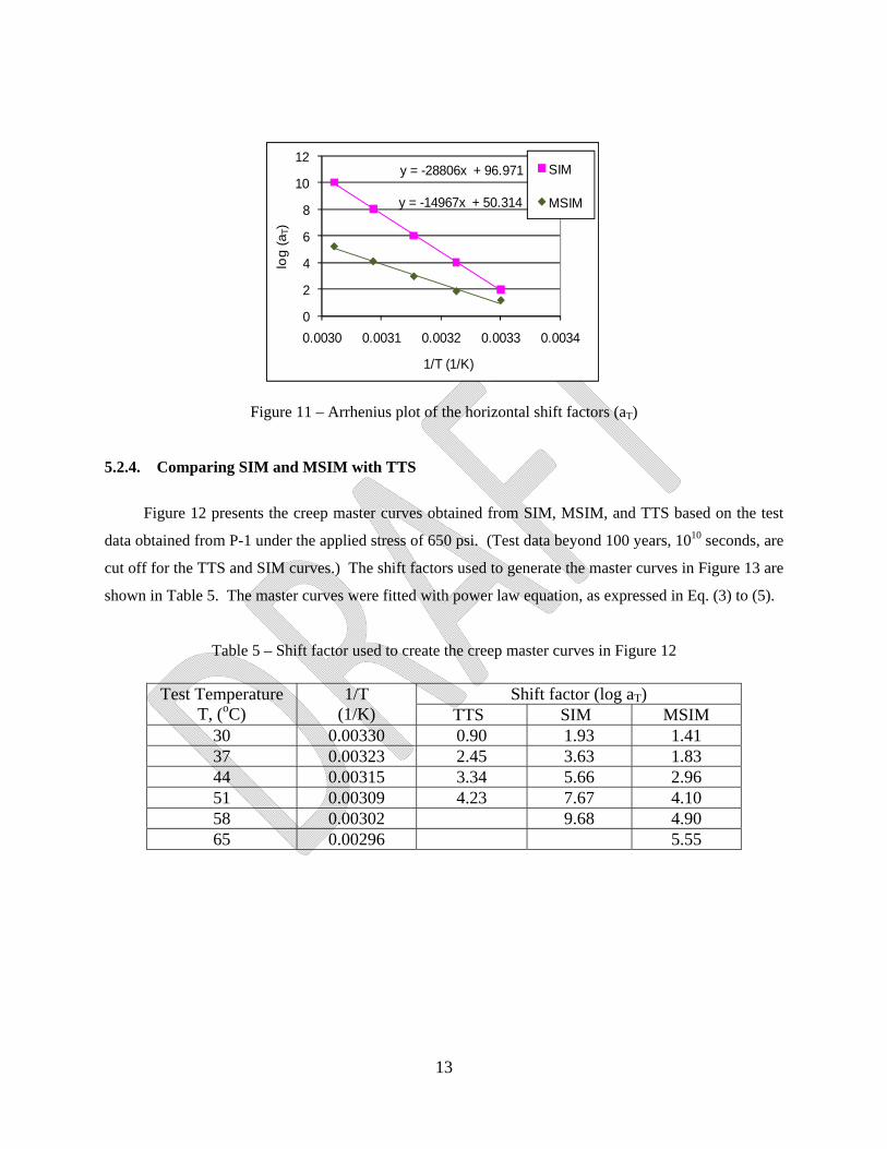
Figure 11 – Arrhenius plot of the horizontal shift factors (aT)

5.2.4. Comparing SIM and MSIM with TTS

Figure 12 presents the creep master curves obtained from SIM, MSIM, and TTS based on the test

data obtained from P-1 under the applied stress of 650 psi. (Test data beyond 100 years, 1010 seconds, are

cut off for the TTS and SIM curves.) The shift factors used to generate the master curves in Figure 13 are

shown in Table 5. The master curves were fitted with power law equation, as expressed in Eq. (3) to (5).

Table 5 – Shift factor used to create the creep master curves in Figure 12

Test Temperature T, (oC)

1/T (1/K)

Shift factor (log aT) TTS SIM MSIM

30 0.00330 0.90 1.93 1.41 37 0.00323 2.45 3.63 1.83 44 0.00315 3.34 5.66 2.96 51 0.00309 4.23 7.67 4.10 58 0.00302 9.68 4.90 65 0.00296 5.55

y = -28806x + 96.971

y = -14967x + 50.314

0

2

4

6

8

10

12

0.0030 0.0031 0.0032 0.0033 0.0034

log

(a

T)

1/T (1/K)

SIM

MSIM

14

Figure 12 – Creep strain master curves at 23oC under 650 psi obtained from TTS, SIM and MSIM

TTS: 0.302 logt 0.4889 (3)

SIM: 0.294 logt 0.8904 (4)

MSIM: 0.300 logt 0.8379 (5)

The master creep curves obtained from SIM and MSIM of this pipe are very similar. The master

creep curve obtained from TTS is lower than those of SIM and MSIM; however, the creep strain rate (the

slope of the creep strain versus log-time) is very similar to those of SIM and MSIM. Therefore the

difference between TTS and SIM is caused by the initial creep strain during the loading. The loading

procedures were different between TTS and SIM. Instantaneous loading was used for tests of TTS, while

gradually loading was applied for tests of SIM. Because stress relaxation was involved in the gradually

loading procedure, the specimen would reach the target stress at a slightly higher strain value.

The activation energy of these three methods is analyzed using the Arrhenius plot, as shown in

Figure 13. In this particular pipe, the TTS and MSIM lines are very similar each other. The activation

energy values are 127, 233, and 113 kJ/mol-K for TTS, SIM, and MSIM, respectively. The activation

energy values of SIM and MSIM are similar to those obtained from the P-3 sample at 500 psi creep test.

With a higher activation energy value, the master curve of SIM can be extended to a longer time period

than MSIM testing under the same test condition.

0

1

2

3

4

5

0 2 4 6 8 10 12

Cre

ep S

trai

n (%

)

Log Time (sec)

TTS

SIM

MSIM

15

Figure 13 – Arrhenius plot of the horizontal shift factors

Although the activation energy of SIM and MSIM is very different, the creep strain master curves

are almost the same at applied stresses of 500 and 600 psi (17% and 22% tensile yield strength) up to 100

years. Yeo and Hsuan (2009) also found that the master curves of SIM and MSIM are very similar at

applied stresses less than 40% ultimate tensile strength of HDPE geogrid. Thus, SIM can be used to

evaluate the long-term modulus of corrugated HDPE pipe, as long as the applied stress is less than 30% of

the yield strength of the pipe material.

5.3. Effect of Specimen Size and Processing on the Creep Behavior

Since the test duration is significantly shorter than the TTS test, SIM was used to investigate the

effect of specimen dimensions and pipe processing on the creep behavior. Three different specimen

configurations were evaluated:

• 2-in wide junction specimen (as shown in Figure 3)

• 1-in wide junction specimen

• 2-in wide specimen taken from the compression molded plaque

Table 6 shows the matrix of tests that were performed using the test procedure of SIM. The test

data were analyzed using a SIM computer program developed by Yeo (2007).

y = -15296x + 51.551

y = -27943x + 93.946

y = -13555x + 45.765

0

2

4

6

8

10

12

0.0029 0.0030 0.0031 0.0032 0.0033 0.0034

Log(

aT)

1/T (1/K)

TTS

SIM

MSIM

16

Table 6 – Information matrix of test using SIM

Manufacturer Pipe Test Specimen Applied Stress (psi)

Test Temperature (oC)

A P-1 (24-in) 2-in wide junction 350, 500, 650, 800 23, 30, 37, 44, 51, 58, 65 1-in wide junction 500

B P-2 (30-in) 2-in wide junction 300, 500, 760, 1140 23, 30, 37, 44, 51, 58, 65 2-in wide plaque 500

B P-3 (48-in) 2-in junction 500 23, 30, 37, 44, 51, 58

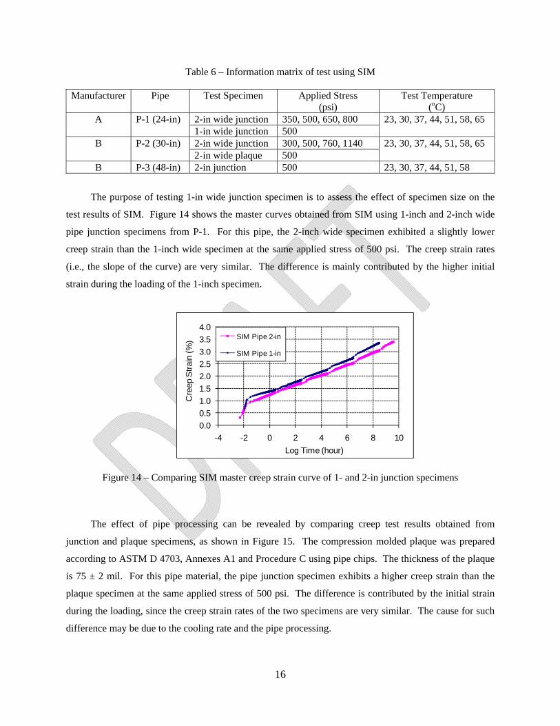
The purpose of testing 1-in wide junction specimen is to assess the effect of specimen size on the

test results of SIM. Figure 14 shows the master curves obtained from SIM using 1-inch and 2-inch wide

pipe junction specimens from P-1. For this pipe, the 2-inch wide specimen exhibited a slightly lower

creep strain than the 1-inch wide specimen at the same applied stress of 500 psi. The creep strain rates

(i.e., the slope of the curve) are very similar. The difference is mainly contributed by the higher initial

strain during the loading of the 1-inch specimen.

Figure 14 – Comparing SIM master creep strain curve of 1- and 2-in junction specimens

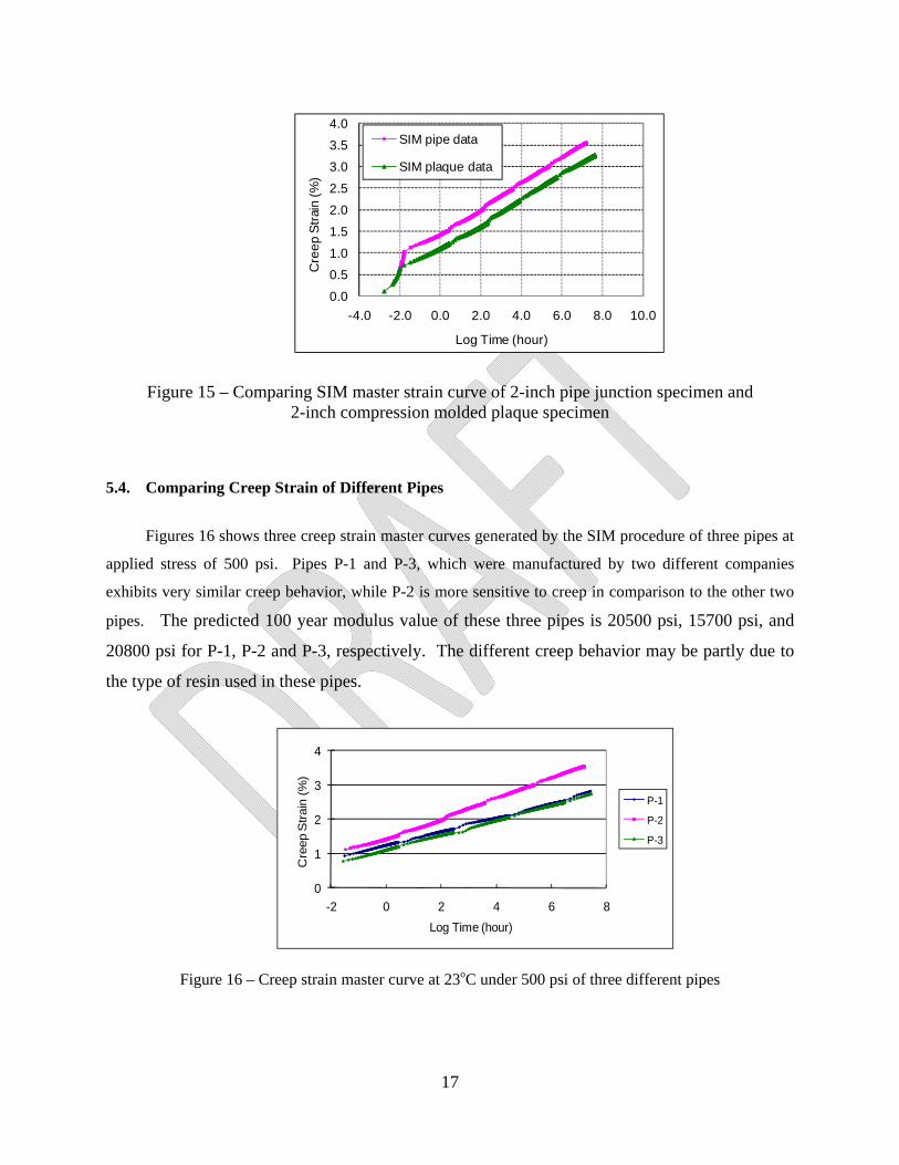
The effect of pipe processing can be revealed by comparing creep test results obtained from

junction and plaque specimens, as shown in Figure 15. The compression molded plaque was prepared

according to ASTM D 4703, Annexes A1 and Procedure C using pipe chips. The thickness of the plaque

is 75 ± 2 mil. For this pipe material, the pipe junction specimen exhibits a higher creep strain than the

plaque specimen at the same applied stress of 500 psi. The difference is contributed by the initial strain

during the loading, since the creep strain rates of the two specimens are very similar. The cause for such

difference may be due to the cooling rate and the pipe processing.

0.0

0.5

1.0

1.5

2.0

2.5

3.0

3.5

4.0

-4 -2 0 2 4 6 8 10

Cre

ep S

trai

n (%

)

Log Time (hour)

SIM Pipe 2-in

SIM Pipe 1-in

17

Figure 15 – Comparing SIM master strain curve of 2-inch pipe junction specimen and 2-inch compression molded plaque specimen

5.4. Comparing Creep Strain of Different Pipes

Figures 16 shows three creep strain master curves generated by the SIM procedure of three pipes at

applied stress of 500 psi. Pipes P-1 and P-3, which were manufactured by two different companies

exhibits very similar creep behavior, while P-2 is more sensitive to creep in comparison to the other two

pipes. The predicted 100 year modulus value of these three pipes is 20500 psi, 15700 psi, and

20800 psi for P-1, P-2 and P-3, respectively. The different creep behavior may be partly due to

the type of resin used in these pipes.

Figure 16 – Creep strain master curve at 23oC under 500 psi of three different pipes

0.0

0.5

1.0

1.5

2.0

2.5

3.0

3.5

4.0

-4.0 -2.0 0.0 2.0 4.0 6.0 8.0 10.0C

ree

p S

trai

n (

%)

Log Time (hour)

SIM pipe data

SIM plaque data

0

1

2

3

4

-2 0 2 4 6 8

Cre

ep S

train

(%

)

Log Time (hour)

P-1

P-2

P-3

18

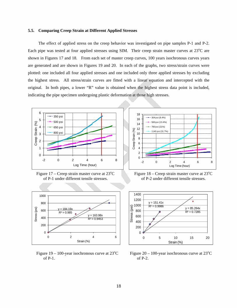
5.5. Comparing Creep Strain at Different Applied Stresses

The effect of applied stress on the creep behavior was investigated on pipe samples P-1 and P-2.

Each pipe was tested at four applied stresses using SIM. Their creep strain master curves at 23oC are

shown in Figures 17 and 18. From each set of master creep curves, 100 years isochronous curves years

are generated and are shown in Figures 19 and 20. In each of the graphs, two stress/strain curves were

plotted: one included all four applied stresses and one included only three applied stresses by excluding

the highest stress. All stress/strain curves are fitted with a linear equation and intercepted with the

original. In both pipes, a lower “R” value is obtained when the highest stress data point is included,

indicating the pipe specimen undergoing plastic deformation at those high stresses.

Figure 17 – Creep strain master curve at 23oC of P-1 under different tensile stresses.

Figure 18 – Creep strain master curve at 23oC of P-2 under different tensile stresses.

0

2

4

6

8

10

12

14

16

18

-2 0 2 4 6 8

Cre

ep S

trai

n (%

)

Log Time (hour)

304 psi (8.4%)

500 psi (13.4%)

760 psi (21%)

1140 psi (31.7%)

0

1

2

3

4

5

6

-2 0 2 4 6 8

Cre

ep S

trai

n (%

)

Log Time (hour)

350 psi

500 psi

650 psi

800 psi

y = 151.41xR² = 0.9986

y = 85.264xR² = 0.7285

0

200

400

600

800

1000

1200

1400

0 5 10 15 20

Str

ess

(psi

)

Strain (%)

Figure 19 – 100-year isochronous curve at 23oC of P-1.

Figure 20 – 100-year isochronous curve at 23oC of P-2.

y = 163.98xR² = 0.9453

y = 184.19xR² = 0.985

0

200

400

600

800

1000

0 2 4 6

Str

ess

(psi

)

Strain (%)

19

The slope of the linear curve represents the 100-year modulus value at any tensile stress up to 650

psi for P-1 and 800 psi for P-2. The 100-year modulus values are included in Table 7, and these values

are lower than the recommended values proposed for corrugated pipe in NCHRP 631 Report, particularly

P-2.

Table 7 –Modulus Obtained from the Isochronous Curve of P-1 and P-2

Pipe 100-Year Modulus P-1 18400 psi P-2 15100 psi

6. SUMMARY

In this project, the long-term modulus of corrugated HDPE pipe was evaluated using two

accelerated creep methods, TTS and SIM. In addition, test data obtained from SIM were analyzed by two

procedures: ASTM procedure D6992 and a modification of the same by use of MSIM analysis. The creep

rates were found to be very similar between TTS and SIM at the tested stresses, verifying that creep test

using SIM can be adopted to determine the 100-year modulus of the corrugated HDPE pipe.

In addition, the creep master curves of SIM and MSIM are basically the same at applied stress

below 30% ultimate yield strength, even though their activation energy values are very different.

Therefore, the data analysis procedure based on SIM can be used to create the master creep curve.

7. STANDARD TEST METHOD

Currently, the test method to evaluate the long-term modulus of corrugated HDPE pipe is FM 5-

577, in which the pipe sample is tested using an accelerated stress relaxation method. Based on the

finding of this study, modification to FM 5-577 is recommended to use an accelerated creep method

(SIM). The proposed draft method is included in Appendix A of this report.

8. RECOMMENDATION IN TESTING

In this study, three pipes from two different manufacturers were evaluated. Two of the pipes, P-1

and P-2 exhibited a large difference in creep sensitivity. The effects of resin type and manufacturing

process on the creep behavior of the pipe were not identified due to limited samples being evaluated.

20

We recommend that pipes to be certified for 100-year service life should be tested at applied stresses of

650, 500 and 350 psi using SIM to generate the 100-year isochronous curve at 23oC. The slope of the

isochronous curve will be the long-term modulus of the pipe.

9. REFERENCES

Jason, L.E., (1985) “Investigation of the long term modulus for buried polyethylene pipes subjected to

constant deflection”, in Advances in Underground Pipeline Engineering, J.K. Jeyapalan, ed., ACSE, New

York.

Chua, K.M., and Lytton, R.L. (1989) “Viscoelastic approach to modeling performance of buried pipes,”

Journal of Transportation Engineering, Vol. 115, No. 3, pp. 253-269.

Zhang, C., and Moore, I.D., (1997a) “Nonlinear mechanical response of high density polyethylene, Part I:

experimental investigation and model evaluation,” Polymer Engineering and Science, Vol. 37, No. 2, pp.

404-413.

Zhang, C., and Moore, I.D., (1997b) “Nonlinear mechanical response of high density polyethylene, Part

II: uniaxial constitutive modeling,” Polymer Engineering and Science, Vol. 37, No. 2, pp. 414-420.

Drozdov, A.D., and Kalamkarow, A.L. (1996) “A constitutive model for nonlinear viscoelastic behavior

of polymers”, Polymer Engineering and Science, Vol. 36, No. 14, pp.1908-1919.

Lai, J., and Bakker, A. (1995) “Analysis of the non-linear creep of high-density polyethylene”, Polymer,

Vol. 36, No. 1, pp. 93-99.

Nielsen, L.E., (1974) Mechanical properties of polymers and composites, Vol. 1, 2, Marcel Dekker Inc., NY. Ferry, J. D. (1980) Viscoelastic properties of polymers, 3rd ed., John Wiley and Sons, NY. Moore, G. R. and Kline, D. E. (1984) Properties and processing of polymers for engineers, Prentice-Hall Inc., Englewood Cliffs, NJ, p209. Painter, P. C., and Coleman. M. M. (1997) Fundamentals of polymer science, 2nd Ed., CRC press, Boca Raton, FL. Thornton, J. S., Paulson, J. N., and Sandri, D. (1998a) “Conventional and stepped isothermal methods for characterizing long term creep strength of polyester geogrids,” 6th international conference on geosynthetics, Atlanta, GA, pp. 691-698.

21

Thornton, J. S., Allen, S. R., Thomas, R. W., and Sandri, D. (1998b) “The stepped isothermal method for time-temperature superposition and its application to creep data on polyester yarn,” 6th international conference on geosynthetics, Atlanta, GA, pp. 699-706. Greenwood, J. H. and Voskamp, W. (2000) “Predicting the long-term strength of a geogrid using the stepped isothermal method,” 2nd European geosynthetics conference (EuroGeo2), Italy, pp. 329-331. Sherby, O. D., and Dorn, J. E. (1958) “Anelastic Creep of Polymethyl Methacrylate,” Journal of mechanics and physics of solids, Vol. 6, pp. 145-162. Hsuan, Y.G., and McGrath, T. (2005) Protocol for Predicting Long-term Service of Corrugated High Density Polyethylene Pipes, Report to Florida Department of Transportation.