tesi di laurea magistrale · tesi di laurea magistrale centralized and distributed generation in a...
TRANSCRIPT
POLITECNICO DI TORINO
CORSO DI LAUREA MAGISTRALE IN INGEGNERIAENERGETICA E NUCLEARE
TESI DI LAUREA MAGISTRALE
Centralized and distributed generation in a district heatingsystem: application of a thermal and fluid-dynamic model
for integrated energy network analysis
RelatoreProf. Pierluigi Leone
CorelatoriDott. Marco CavanaDott. Enrico Vaccariello
CandidatoAndrea Cascavilla
A.A. 2019/2020

Ad AlessiaAlla mia famiglia

Abstract
The aim of this work is to implement and apply a model to evaluate thethermo-fluid dynamic behaviour of district heating networks, with the help ofgraph theory and SIMPLE algorithm.
The purpose of this implementation is to study the feasibility of the sub-stitution of natural gas users with district heating users, in order to study thepossibility of an integrate energy network analysis.
The first part of the work is dedicated to the numerical implementation,with the help of software Matlab, of the physical problem. A generic networkis analyzed, with consequent results and validation of the model.
Once the model is validated, it has been applied to a real configuration:a case study of a gas network in an urban area. A substitution of naturalgas load for heating with district heating is supposed. The installation of thenetwork is studied in two different configurations: centralized heat generationand distributed heat generation.
In the first case a cogeneration plant of 90 MWe is chosen, where theheat generated is provided to the district heating network and the electricitygenerated is sent to the grid.In the second case the power of the cogeneration plant is halved, the supplytemperature of the grid is decreased and 21 thermal boosters are applied instrategic nodes. These thermal boosters are linked to the gas network andelectricity grid, and here space for an integrate energy network analysis is left.
The study ends with the analysis of Carbon Dioxide emissions, primaryenergy saving and economic analysis of the two different installation configu-rations.
1

CONTENTS
Contents
1 Introduction 8
2 Numerical model of district heating networks 102.1 Physical problem . . . . . . . . . . . . . . . . . . . . . . . . . . . . . 102.2 Numerical problem . . . . . . . . . . . . . . . . . . . . . . . . . . . . 11
2.2.1 Fluid dynamic problem . . . . . . . . . . . . . . . . . . . . . . 122.2.2 SIMPLE algorithm . . . . . . . . . . . . . . . . . . . . . . . . 162.2.3 Thermal numerical problem . . . . . . . . . . . . . . . . . . . 17
2.3 Results validation . . . . . . . . . . . . . . . . . . . . . . . . . . . . . 222.3.1 Mass flow rates . . . . . . . . . . . . . . . . . . . . . . . . . . 242.3.2 Temperatures . . . . . . . . . . . . . . . . . . . . . . . . . . . 242.3.3 Pressure drop . . . . . . . . . . . . . . . . . . . . . . . . . . . 27
3 Analysis on the network 323.1 Return network . . . . . . . . . . . . . . . . . . . . . . . . . . . . . . 323.2 Load variation analysis . . . . . . . . . . . . . . . . . . . . . . . . . . 343.3 Heat Losses . . . . . . . . . . . . . . . . . . . . . . . . . . . . . . . . 35
3.3.1 Heat losses in steady state . . . . . . . . . . . . . . . . . . . . 353.3.2 Heat losses in transient condition . . . . . . . . . . . . . . . . 373.3.3 Sensitivity analysis with ground temperature . . . . . . . . . . 38
4 Case study: introduction of district heating in a gas network 404.1 Urban area description . . . . . . . . . . . . . . . . . . . . . . . . . . 404.2 Consumption profiling . . . . . . . . . . . . . . . . . . . . . . . . . . 43
4.2.1 Daily consumption . . . . . . . . . . . . . . . . . . . . . . . . 434.2.2 Hourly profiling . . . . . . . . . . . . . . . . . . . . . . . . . . 464.2.3 Calculation of thermal demand and mass flow rate . . . . . . 47
4.3 Application of case study at the numerical model . . . . . . . . . . . 494.3.1 Switching mode . . . . . . . . . . . . . . . . . . . . . . . . . . 494.3.2 Continuous operation mode . . . . . . . . . . . . . . . . . . . 564.3.3 Annual results analysis . . . . . . . . . . . . . . . . . . . . . . 63
4.4 Production energy system design . . . . . . . . . . . . . . . . . . . . 644.4.1 Combined heat and power (CHP) technologies . . . . . . . . . 654.4.2 Case 1: centralized generation . . . . . . . . . . . . . . . . . . 694.4.3 Case 2: distributed generation . . . . . . . . . . . . . . . . . . 70
4.5 Primary energy and CO2 emissions calculation . . . . . . . . . . . . . 744.5.1 Case 0 . . . . . . . . . . . . . . . . . . . . . . . . . . . . . . . 744.5.2 Case 1: substitution with centralized generation . . . . . . . . 764.5.3 Case 2: substitution with distributed generation . . . . . . . . 77
2

CONTENTS
5 Economic Analysis 795.1 Case 1: Centralized generation . . . . . . . . . . . . . . . . . . . . . . 81
5.1.1 CAPEX . . . . . . . . . . . . . . . . . . . . . . . . . . . . . . 815.1.2 OPEX . . . . . . . . . . . . . . . . . . . . . . . . . . . . . . . 845.1.3 Cashflow Analysis . . . . . . . . . . . . . . . . . . . . . . . . . 87
5.2 Case 2: Distributed Generation . . . . . . . . . . . . . . . . . . . . . 89
6 Comparison between the configurations 946.1 Energy saving and CO2 emissions . . . . . . . . . . . . . . . . . . . . 946.2 Economic assessment . . . . . . . . . . . . . . . . . . . . . . . . . . . 98
7 Conclusions and Future Developments 1017.1 Future developments . . . . . . . . . . . . . . . . . . . . . . . . . . . 102
3

LIST OF FIGURES
List of Figures
1 Control volume taken into account [12] . . . . . . . . . . . . . . . . . 182 Specific control volume taken into account for equation (33) [12] . . . 193 Control volume taken into account [12] . . . . . . . . . . . . . . . . . 214 Network taken as an example . . . . . . . . . . . . . . . . . . . . . . 235 Temperature at each node . . . . . . . . . . . . . . . . . . . . . . . . 256 Grid convergence . . . . . . . . . . . . . . . . . . . . . . . . . . . . . 257 Temperature of the last node in time with three different grid refine-
ments . . . . . . . . . . . . . . . . . . . . . . . . . . . . . . . . . . . 268 Pressure value at each node . . . . . . . . . . . . . . . . . . . . . . . 279 Grid convergence for pressure . . . . . . . . . . . . . . . . . . . . . . 2810 Residual linked to the momentum equation . . . . . . . . . . . . . . . 2911 Residual linked to the continuity equation . . . . . . . . . . . . . . . 2912 Pressure calculated with momentum equation, without SIMPLE . . . 3013 Heat exchanger from district heating to the users [14] . . . . . . . . . 3214 Temperature at each node . . . . . . . . . . . . . . . . . . . . . . . . 3315 Pressure at each node . . . . . . . . . . . . . . . . . . . . . . . . . . . 3316 Temperature profile at each node with different heat demand . . . . . 3417 Variation of pressures with the load . . . . . . . . . . . . . . . . . . . 3518 Heat losses for each branch of supply line . . . . . . . . . . . . . . . . 3619 Heat losses for each branch of return line . . . . . . . . . . . . . . . . 3620 Heat losses in time of supply line . . . . . . . . . . . . . . . . . . . . 3721 Heat losses in time of return line . . . . . . . . . . . . . . . . . . . . 3822 Heat losses dependent on ground temperature . . . . . . . . . . . . . 3823 Urban area topology . . . . . . . . . . . . . . . . . . . . . . . . . . . 4024 Natural gas volumetric flow rate . . . . . . . . . . . . . . . . . . . . . 4125 Legend of natural gas flow rate . . . . . . . . . . . . . . . . . . . . . 4126 Natural gas consumption for each node . . . . . . . . . . . . . . . . . 4227 Users of the network . . . . . . . . . . . . . . . . . . . . . . . . . . . 4228 Climate zone in Italy . . . . . . . . . . . . . . . . . . . . . . . . . . . 4429 Legend of climate zone in Italy and corresponding Degree Day values 4430 Total annual consumption of the users . . . . . . . . . . . . . . . . . 4631 Weekly consumption of the users . . . . . . . . . . . . . . . . . . . . 4632 Hourly consumption percentage with respect to total daily consumption 4733 Total hourly power demand and hourly mass flow rate . . . . . . . . 4934 Total plant load in Turin [29] . . . . . . . . . . . . . . . . . . . . . . 5035 Substation scheme in a district heating network [30] . . . . . . . . . . 5136 Diameters and length of pipelines . . . . . . . . . . . . . . . . . . . . 5237 Mass flow rate for each node, with peak mass flow rate . . . . . . . . 5238 Pressure and velocity of switching mode . . . . . . . . . . . . . . . . 5339 Heat losses in time for supply and return line . . . . . . . . . . . . . 54
4

LIST OF FIGURES
40 Thermal power in time provided to the network . . . . . . . . . . . . 5441 Temperature at the nodes after 2 hours from the switching . . . . . . 5542 Temperature at the nodes after 2 hours from the switching on . . . . 5543 Temperature in steady state of supply and return line . . . . . . . . . 5644 Temperature in steady state and velocities of supply line . . . . . . . 5745 Temperature in steady state of return line . . . . . . . . . . . . . . . 5746 Heat losses of each branch at steady state for supply and return line . 5847 Heat losses for each branch . . . . . . . . . . . . . . . . . . . . . . . . 5848 Mass flow rate and temperature in a day of January for a non indus-
trial node . . . . . . . . . . . . . . . . . . . . . . . . . . . . . . . . . 5949 Mass flow rate and temperature in a day of January for an industrial
node . . . . . . . . . . . . . . . . . . . . . . . . . . . . . . . . . . . . 5950 Maximum and minimum pressure profile in a day of January . . . . . 6051 Pressure along the network . . . . . . . . . . . . . . . . . . . . . . . . 6152 Pressure along the supply line . . . . . . . . . . . . . . . . . . . . . . 6153 Daily profile of thermal losses . . . . . . . . . . . . . . . . . . . . . . 6254 Daily profile of thermal power and percentage of losses . . . . . . . . 6255 SIMPLE algorithm residuals . . . . . . . . . . . . . . . . . . . . . . . 6256 Pressure drop on supply line every day of the year . . . . . . . . . . . 6357 Energy provided to the system and total thermal losses along the year 6458 Total thermal losses along the year with correspondent percentage on
the total energy provided . . . . . . . . . . . . . . . . . . . . . . . . . 6459 CHP production operating principle . . . . . . . . . . . . . . . . . . . 6660 An internal combustion engine . . . . . . . . . . . . . . . . . . . . . . 6761 A gas turbine . . . . . . . . . . . . . . . . . . . . . . . . . . . . . . . 6862 CHP technologies in function of available sizes and electrical efficiency
[31] . . . . . . . . . . . . . . . . . . . . . . . . . . . . . . . . . . . . . 6963 Cumulative curve of thermal demand . . . . . . . . . . . . . . . . . . 6964 Configuration of the plant . . . . . . . . . . . . . . . . . . . . . . . . 7065 Yellow points identify the grid zones where the generated generation
is installed . . . . . . . . . . . . . . . . . . . . . . . . . . . . . . . . . 7066 Temperature profile of supply line in case 2 . . . . . . . . . . . . . . . 7167 Temperature of supply line in case 2 . . . . . . . . . . . . . . . . . . 7168 Total thermal losses along the year with correspondent percentage on
the total energy provided . . . . . . . . . . . . . . . . . . . . . . . . . 7269 Cumulative curve of thermal demand for the plant . . . . . . . . . . . 7270 Cumulative curve of thermal demand for a non industrial user . . . . 7371 Cumulative curve of thermal demand for an industrial user . . . . . . 7372 Configuration of the plant . . . . . . . . . . . . . . . . . . . . . . . . 7373 Commercial micro-turbines . . . . . . . . . . . . . . . . . . . . . . . . 7474 Parameters taken into consideration for economic analysis . . . . . . 8275 Economic costs provided by GSE [17] . . . . . . . . . . . . . . . . . . 82
5
LIST OF FIGURES
76 Unit installation cost for distribution network [16] [15] . . . . . . . . 8377 Total installation cost for distribution network . . . . . . . . . . . . . 8378 Cash flow analysis (case 1) . . . . . . . . . . . . . . . . . . . . . . . . 8879 Cumulative Cash Flow for every year of system lifetime (case 1) . . . 8880 Parameters taken into consideration for economic analysis . . . . . . 8981 Unit investment cost for the construction of gas turbines [23] . . . . . 9182 Unit Operation & Maintenance cost for gas turbines [23] . . . . . . . 9183 Cash flow analysis for case of distributed generation . . . . . . . . . . 9384 Cumulative Cash Flow in time for distributed generation case . . . . 9385 Primary energy consumption of the three configurations . . . . . . . . 9486 CO2 emissions for the three configurations . . . . . . . . . . . . . . . 9587 CO2 emitted for heating purpose . . . . . . . . . . . . . . . . . . . . 9688 Index of efficiency: how much useful energy is provided to the system
[MWh] with one toe of primary energy . . . . . . . . . . . . . . . . . 9789 Compared NPV for the two configurations . . . . . . . . . . . . . . . 9890 Payback Period of the two configurations . . . . . . . . . . . . . . . . 9991 Some details of economic analysis . . . . . . . . . . . . . . . . . . . . 9992 Thermal losses in a year of the two configurations . . . . . . . . . . . 10193 Thermal demand of the boosters . . . . . . . . . . . . . . . . . . . . . 10394 Heat pump water heater scheme [32] . . . . . . . . . . . . . . . . . . 10395 Solid Oxide Fuel Cell basic operation scheme . . . . . . . . . . . . . . 10496 Electricity output of each booster . . . . . . . . . . . . . . . . . . . . 10497 Natural gas consumption of each booster . . . . . . . . . . . . . . . . 105
6

LIST OF TABLES
List of Tables
1 Maximum thermal demand of the users . . . . . . . . . . . . . . . . . 232 Maximum thermal demand of the users . . . . . . . . . . . . . . . . . 243 Error of the 3 grids with respect to the more refined one . . . . . . . 264 Error of the 3 grids with respect to the more refined one . . . . . . . 285 Percentage error of pressure obtained with SIMPLE with respect to
pressure obtained with equation (19) . . . . . . . . . . . . . . . . . . 316 Picking class from arera [27] . . . . . . . . . . . . . . . . . . . . . . . 437 Gas category of use [27] . . . . . . . . . . . . . . . . . . . . . . . . . 458 Energy/Heat ratio for different CHP technologies . . . . . . . . . . . 669 Emission factor from national inventory of UNFCCC (mean 2016-2018) 75
7

1 Introduction
1 Introduction
District heating systems can be defined as the distribution of thermal energy from
a central source to residential or industrial activities.
In the last 50 years this technology spread all over the world, specially in USA,
Europe, Japan, China and Korea. Only in Europe it reaches more than 60 million
people.
Various sources of heat supply these kind of systems: cogeneration, industrial waste
heat, incinerators, solar energy, biomass. Thanks to these sources district heating is
more environmentally-friendly than boilers in single houses: every year more than
5000 district heating systems in Europe, covering more than 10% of total European
heat demand [2], contributes to avoid 3-4% of CO2 emissions [1].
This situation makes district heating of topical interest, in the field of energetic
transition and environmental issue. For this reason research in this area is going
toward an integration with green energy, that brings in the study not only district
heating network, but also electricity grid and gas network. A lot of publications
address the problem of synergy for all the energetic networks. In this regard the 4th
generation district heating is a central point [3]: the district heating is integrated
with smart technologies, smart metering, storage and renewables, in order to obtain
a more green and efficient system.
In the area of smart energy, analyses on the prosumers in district heating have
been conducted [4], studying the impact of including someone who both consumes
and produces heat in a local network. Nevertheless, for the objective of this work, the
most interesting studies are those ones involving other networks. The integration in
smart energy systems, in fact, allows solutions of low-cost storage and consequently a
participation in balancing fluctuating renewable energy sources [5], like the solution
proposed by Rehman et al. [6], in which a photovoltaic distributed and three solar
thermal district heating systems are compared, showing that the first overcomes all
the others in terms of economic and environmental aspects.
8

1 Introduction
A solution of great interest is the combination of combined heat and power (CHP)
plants together with large scale heat pumps in district heating systems to balance
intermittent renewable power production [7]. It is possible to use power production
and consumption to balance both surplus and deficit in the electric power market.
This is the case of integration of the three energetic networks, whose behaviour can
be analyzed by computational studies.
Remaining in the field of green and circular economy, a form of integration is also
using biogas from wastewater treatment plant as a source of heat for the network
[8].
Concerning numerical design of district heating network several studies have been
conducted. In this work the method proposed by Sciacovelli, Verda and Borchiellini
[9] has been taken as reference. This method allowed to implement numerical codes
in Matlab for the calculation, in steady and unsteady state, of temperature, mass
flow rate and pressure of the district heating network taken into account.
9

2 Numerical model of district heating networks
2 Numerical model of district heating networks
2.1 Physical problem
The analysis of a district heating network involves the prediction of mass flow rate,
temperature and pressure, evaluated in some specific points, according to what is
needed. The purpose of this study is the modeling of the behaviour of the district
heating network in connection with electrical grid and gas network.
A physical and then numerical model is necessary to assess all the things above
mentioned, because installing measuring equipment on the networks to measure
the quantities needed at various locations would be too expensive, intrusive and
therefore complicated.
The model chosen is a quasi-dynamic model [10]: the thermal problem is simu-
lated in unsteady state, while the fluid-dynamic formulation is considered stationary.
This because the hydraulic perturbations are transferred in a time of few seconds,
which is even smaller than the time step adopted. On the contrary, thermal per-
turbations travel at the fluid velocity, so the effect are slower and remarkable for
this study. The approach used in this study follows the one proposed by Sciacovelli,
Verda and R.Borchiellini [9].
The model is based on the conservation equations:
1. CONTINUITY EQUATION
In differential form:
dρ
dt+ ρ∇ · u = 0 , (1)
which in case of one-dimensional formulation becomes:
∂ρ
∂t+∂(ρv1)
ρx1
= 0 . (2)
2. MOMENTUM EQUATION
10
2.2 Numerical problem
In differential form the equation is
ρDv
Dt= −∇p−∇ · τ + F , (3)
that, written for one dimension along x1 direction, becomes:
ρ∂v1
∂t+ ρv1
∂v
∂x1
= − ∂p
∂x1
− Ffr + F1 , (4)
where Ffr identifies distributed pressure drop and F1 = ρ · gx1 −Flocal +Fpump
is the source term, including gravity, local pressure drop and pressure rise due
to pumps.
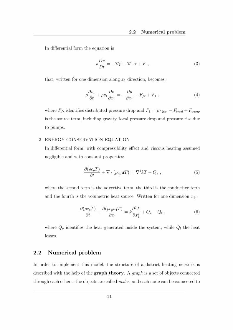
3. ENERGY CONSERVATION EQUATION
In differential form, with compressibility effect and viscous heating assumed
negligible and with constant properties:
∂(ρcpT )
∂t+∇ · (ρcpuT ) = ∇2kT +Qs , (5)
where the second term is the advective term, the third is the conductive term
and the fourth is the volumetric heat source. Written for one dimension x1:
∂(ρcpT )
∂t+∂(ρcpu1T )
∂x1
= k∂2T
∂x21
+Qv −Ql , (6)
where Qv identifies the heat generated inside the system, while Ql the heat
losses.
2.2 Numerical problem
In order to implement this model, the structure of a district heating network is
described with the help of the graph theory. A graph is a set of objects connected
through each others: the objects are called nodes, and each node can be connected to
11

2.2 Numerical problem
other nodes through multiple links, called branches. For a district heating network,
nodes correspond to junctions, and branches, elements that link to different nodes,
correspond to pipes, ducts and similar components. The best way to describe the
network topology of a flow network, i.e. the interconnections between nodes and
branches, is the incidence matrix A, where the general element Aij is equal to:
• 1, if the i-th node is the inlet node of j-th branch;
• -1, if the i-th node is the outlet node of j-th branch;
• 0, if there is no connection between node i and branch j.
It follows that matrix A has a number of rows equal to the number of nodes and
number of columns equal to the number of branches.
2.2.1 Fluid dynamic problem
In order to calculate the mass flow rates in the network mass conservation equation
is needed. If equation (1) is integrated over a control volume CV that includes one
node and half of each branch connected to it, one can obtain:
dM
dt+
NB∑j=1
ρj · v1,j · Sj = 0 , (7)
where M is the mass of fluid in the control volume, NB is the total number of
branches, Sj is the j-th branch cross section.
In order to consider a possible injection or extraction of the fluid from a node, the
term Gext is added, which represent the mass flow rates exiting from the junctions
(in this case it is a positive term) or entering (negative term). Considering also the
definition of mass flow rate it is obtained: the following expression:
dM
dt+
NB∑j=1
Gj +Gext = 0 , (8)
12
2.2 Numerical problem
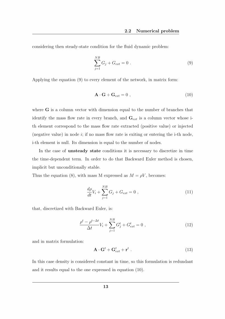
considering then steady-state condition for the fluid dynamic problem:
NB∑j=1
Gj +Gext = 0 . (9)
Applying the equation (9) to every element of the network, in matrix form:
A ·G + Gext = 0 , (10)
where G is a column vector with dimension equal to the number of branches that
identify the mass flow rate in every branch, and Gext is a column vector whose i-
th element correspond to the mass flow rate extracted (positive value) or injected
(negative value) in node i; if no mass flow rate is exiting or entering the i-th node,
i-th element is null. Its dimension is equal to the number of nodes.
In the case of unsteady state conditions it is necessary to discretize in time
the time-dependent term. In order to do that Backward Euler method is chosen,
implicit but unconditionally stable.
Thus the equation (8), with mass M expressed as M = ρV , becomes:
dρ
dtVi +
NB∑j=1
Gj +Gext = 0 , (11)
that, discretized with Backward Euler, is:
ρt − ρt−∆t
∆tVi +
NB∑j=1
Gtj +Gt
ext = 0 , (12)
and in matrix formulation:
A ·Gt + Gtext + rt . (13)
In this case density is considered constant in time, so this formulation is redundant
and it results equal to the one expressed in equation (10).
13
2.2 Numerical problem
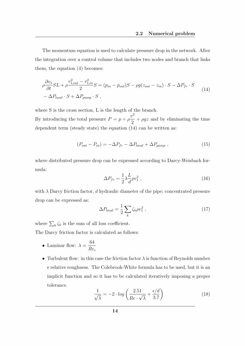
The momentum equation is used to calculate pressure drop in the network. After
the integration over a control volume that includes two nodes and branch that links
them, the equation (4) becomes:
ρ∂v1
∂tSL+ ρ
v21,out − v2
1,in
2S = (pin − pout)S − ρg(zout − zin) · S −∆Pfr · S
−∆Plocal · S + ∆Ppump · S ,
(14)
where S is the cross section, L is the length of the branch.
By introducing the total pressure P = p + ρv2
2+ ρgz and by eliminating the time
dependent term (steady state) the equation (14) can be written as:
(Pout − Pin) = −∆Pfr −∆Plocal + ∆Ppump , (15)
where distributed pressure drop can be expressed according to Darcy-Weisbach for-
mula:
∆Pfr =1
2λL
dρv2
1 , (16)
with λ Darcy friction factor, d hydraulic diameter of the pipe; concentrated pressure
drop can be expressed as:
∆Plocal =1
2
∑k
ζkρv21 , (17)
where∑
h ζk is the sum of all loss coefficient.
The Darcy friction factor is calculated as follows:
• Laminar flow: λ =64
Ree
• Turbulent flow: in this case the friction factor λ is function of Reynolds number
e relative roughness. The Colebrook-White formula has to be used, but it is an
implicit function and so it has to be calculated iteratively imposing a proper
tolerance.1√λ
= −2 · log(
2.51
Re ·√λ
+ε/d
3.7
)(18)
14

2.2 Numerical problem
Substituting then equations (16) and (17) in (15) and applying at the control volume
that includes a branch and the two nodes at the extremities it is obtained:
(Pi−1 − Pi) =1
2
G2j
ρS2j
(λjLj
dj+∑k
ζk,j)−∆Ppump,j (19)
Applying equation (19) at every branch j of the network and defining hydraulic
resistance as Rj =1
2
Gj
ρS2j
(λjLj
dj+∑
k ζk,j) the matrix formulation of the momentum
equation is obtained:
AT ·P = R ·G− t , (20)
where P is a column vector with dimension equal to the number of nodes which
identifies the value of total pressure at each node, t identifies for each branch the
pressure rise due to the pumps. Deriving G from (20) and defining hydraulic con-
ductance matrix as Y = R−1:
G = Y ·AT ·P + Y · t . (21)
In unsteady state condition from equation (14), applying Backward Euler and
with constant density it is obtained:
(Pi−1 − Pi)t = Rt
j ·Gtj +Bt
j ·Gtj −∆P t
pump,j −X tj , (22)
where Btj =
LjSj
∆tand X t
j = −ρtLjSj
∆t
Gt−∆tj
ρt−∆t. Now matrix formulation is applied,
with Y′ = Rt + Bt and the mass flow rate is derived from the equation:
Gt = Y′t ·AT ·Pt + Y′t · tt + Y′t ·Xt (23)
The problem with equations (21) and (23) is that matrix Y is a function of the mass
flow rate, which is the unknown. Moreover the pressure is not known. In order to
solve this non-linearity the iterative SIMPLE algorithm must be used.
15

2.2 Numerical problem
2.2.2 SIMPLE algorithm
The SIMPLE (Semi-Implicit Method for Pressure Linked Equation) [9] algorithm is
based on a guess and correction method, and the procedure to be followed is:
1. Guess the pressure vector, that is identified as P* and the under-relaxation
factors for pressure αP and mass flow rate αG. The optimal values of these
two number are unfortunately strongly dependent on the typology of network
considered.
2. Calculation of G* with fixed-point method, which is an iterative process needed
due to the non-linearity of equation (21). It allows to calculate G* thanks to
its value at the previous iteration:
G∗k+1 = Y(G∗x) ·AT ·P∗ + Y(G∗x) · t , (24)
where, in order to avoid divergence,
G∗x = a1G∗k + a2G
∗k−1 , (25)
with a1 + a2 = 1.
3. Correction of mass flow rate and pressure:
Gcorr = G−G∗ (26)
Pcorr = P−P∗ (27)
By substitution of the two previous equations in (21), after the approximation
of Y with Y*, it is obtained:
Gcorr = Y∗ ·AT · (P−P∗) = Y∗ ·AT ·Pcorr . (28)
16

2.2 Numerical problem
4. Calculation of matrices H and b, derived as follows: from equation (10) and
(26) it is obtained
A ·Y∗ ·AT ·Pcorr = −A ·G∗ −Gext , (29)
and, consequently
H ·Pcorr = b , (30)
where the above mentioned matrices are defined as H = A · Y∗ · AT and
b = −A ·G∗ −Gext.
5. Setting of boundary conditions of fluid-dynamic problem, that are about mass
flow rate and pressure:
• Exiting or entering mass flow rate are imposed simply defining the vector
Gext, as explained in section 2.2.1.
• In order to impose pressure at the nodes, it is necessary, at first, set to
the i-th element (corresponding to the i-th node) of P∗ at the desired
value, and then to modify at every iteration H and b in such a way that
the i-th element of Pcorr is null. To do that, the i-th row of H must be
composed of null elements except for i-th one, that must be set to a value
different from zero, while i-th element of vector b must be zero.
2.2.3 Thermal numerical problem
The solution of this problem is needed in order to analyse the behaviour of the tem-
perature at each node. For this purpose the energy equation (6) is applied to all the
nodes of the network. The control volume considered includes the junction, node
and half of the pipe linked to the junction (see figure 1), and when the different
streams gather into the node, adiabatic and perfect mixing is assumed, and heat
losses are ascribed to the branches.
17
2.2 Numerical problem
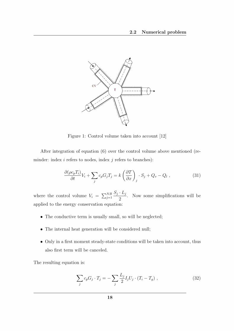
Figure 1: Control volume taken into account [12]
After integration of equation (6) over the control volume above mentioned (re-
minder: index i refers to nodes, index j refers to branches):
∂(ρcpTi)
∂tVi +
∑j
cpGjTj = k
(∂T
∂x
)j
· Sj +Qv −Ql , (31)
where the control volume Vi =∑NB
j=1
Sj · Lj
2. Now some simplifications will be
applied to the energy conservation equation:
• The conductive term is usually small, so will be neglected;
• The internal heat generation will be considered null;
• Only in a first moment steady-state conditions will be taken into account, thus
also first term will be canceled.
The resulting equation is:
∑j
cpGj · Tj = −∑j
Lj
2IjUj · (Ti − Tg) , (32)
18

2.2 Numerical problem
where the right side is the expression of heat losses Ql, with Ij perimeter of the duct
j perpendicular to the water flow, Uj the heat transmission coefficient of branch j
and Tg the temperature of the ground. The length is divided by 2 because only half
of the length of the branches is considered, as already explained.
The equation (32) is now applied to the node i in figure 2. In order to do that
it is necessary to apply an appropriate scheme that evaluates the temperatures at
the boundary of the control volume (Tj), since temperatures are defined only at the
node. For this purpose upwind scheme is adopted, this means that the value of the
temperature at the boundary is assumed equal to the temperature of upstream node.
The upwind scheme has two important properties: it is unconditionally bounded
and it takes into account the flow direction so the transportiveness of the mesh is
guaranteed. The problem is that this method is first order accurate so numerical
diffusion can be present.
Figure 2: Specific control volume taken into account for equation (33) [12]
cp(Gj+1 +Gj+3) · Ti − cpGjTi−1 − cpGj+2Ti+2 = −(∑j
Lj
2IjUj) · (Ti − Tg) , (33)
19

2.2 Numerical problem
where
∑j
LjIjUj = LjIjUj + Lj+1Ij+1Uj+1 + Lj+2Ij+2Uj+2 + Lj+3Ij+3Uj+3. (34)
Now the temperature terms are gathered:
[cp(Gj+1 +Gj+3 +∑j
Lj
2IjUj)] ·Ti− [cpGj−1] ·Ti−1− [cpGj+2] ·Ti+2 = (
∑j
Lj
2IjUj) ·Tg
(35)
It is now possible to build the stiffness matrix K, a square matrix of dimension nxn
with n number of nodes in the network. The element km,p identifies the coefficient
of temperature Tp at the node m. After defining T as the column vector whose
elements are the temperature at the nodes and f the column vector of known terms,
the equation (35) can be written in matrix formulation:
K ·T = f . (36)
In order to solve the problem it is necessary to impose the boundary conditions:
• INPUT NODES
It is necessary to set a condition of imposed temperature (Dirichlet boundary
condition), i.e. setting a value of temperature at the input node, let us call
it node m. In order to do that, all the element of the m-th row of matrix K
should be set equal to zero, except the m-th element (km,m) that should be set
equal to 1. After that, the value of m-eh element of vector f must correspond
to the temperature desired.
• OUTPUT NODES
Here a condition of imposed flux (Robin boundary condition) is required. More
precisely, the thermal losses of the fluid flowing in the branch that precedes the
output node (i.e. between the two nodes) are set equal to the thermal losses
20
2.2 Numerical problem
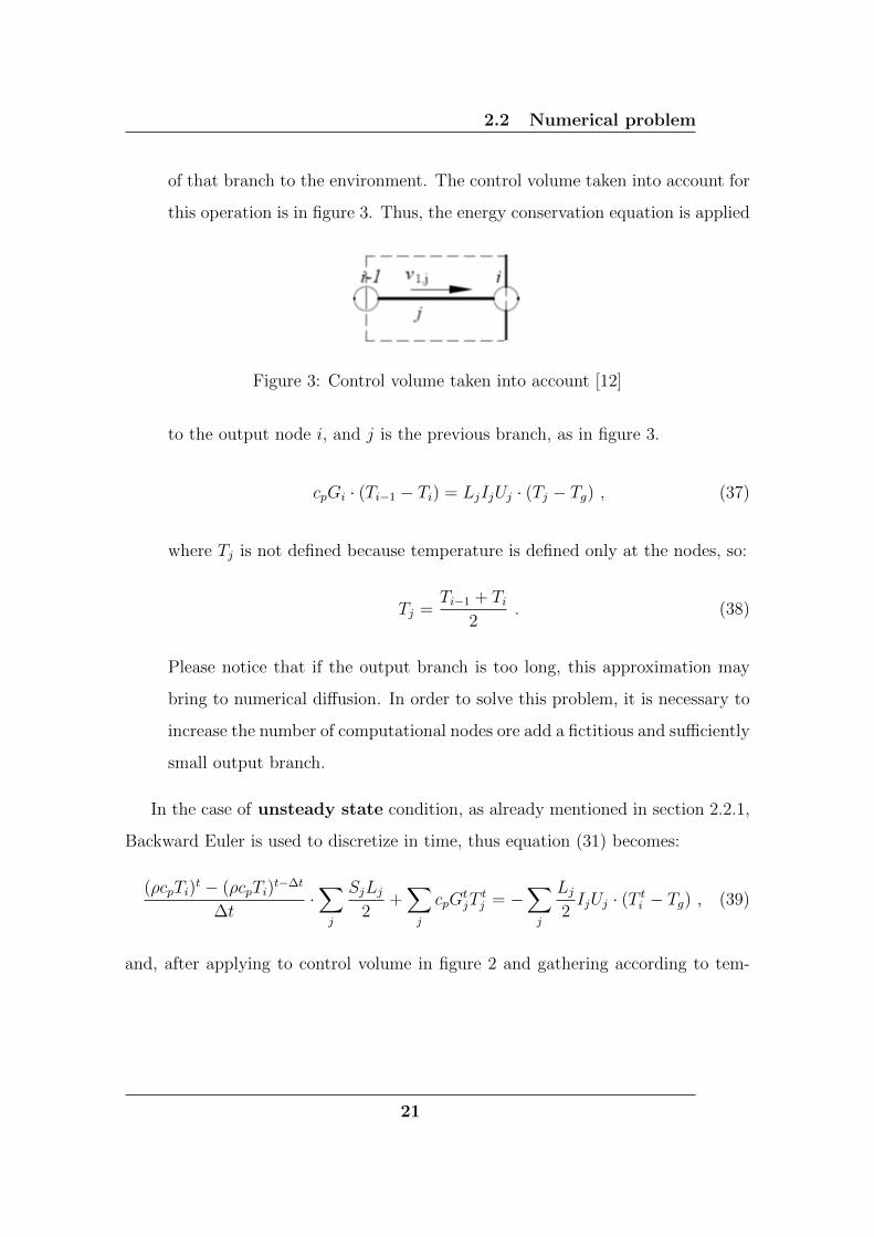
of that branch to the environment. The control volume taken into account for
this operation is in figure 3. Thus, the energy conservation equation is applied
Figure 3: Control volume taken into account [12]
to the output node i, and j is the previous branch, as in figure 3.
cpGi · (Ti−1 − Ti) = LjIjUj · (Tj − Tg) , (37)
where Tj is not defined because temperature is defined only at the nodes, so:
Tj =Ti−1 + Ti
2. (38)
Please notice that if the output branch is too long, this approximation may
bring to numerical diffusion. In order to solve this problem, it is necessary to
increase the number of computational nodes ore add a fictitious and sufficiently
small output branch.
In the case of unsteady state condition, as already mentioned in section 2.2.1,
Backward Euler is used to discretize in time, thus equation (31) becomes:
(ρcpTi)t − (ρcpTi)
t−∆t
∆t·∑j
SjLj
2+∑j
cpGtjT
tj = −
∑j
Lj
2IjUj · (T t
i − Tg) , (39)
and, after applying to control volume in figure 2 and gathering according to tem-
21

2.3 Results validation
peratures:[ρcp2∆t· (∑j
SjLj) + cp · (Gtj+1 + gtj+3) +
∑j
Lj
2IjUj
]· T t
i + [−cpGtj] · T t
i−1+
+ [−cpGtj+2] · T t
i+2 = (∑j
Lj
2IjUj) · Tg +
ρcp2∆t· (∑j
SjLj) · T t−∆ti .
(40)
This can be expressed in matrix formulation, as in steady-state case:
(K + C) ·Tt = f + C ·Tt−∆t . (41)
At this point, the boundary condition of input nodes is unchanged, while at the
output node equation (37), by applying always Backward Euler, becomes:
[ρcp2∆t
SjLj + cpGj +LjIjUj
2
]· T t
i +
[ρcp2∆t
SjLj − cpGj +LjIjUj
2
]· T t
i−1 =
= LjIjUj · Tg +ρcp∆t
SjLj ·T t−∆ti + T t−∆t
i−1
2.
(42)
2.3 Results validation
Once the behaviour of the district heating network can be simulated, it is necessary
to verify if the results obtained are realistic. In order to do that, the following
fictitious network has been created.
Node 1 is the inlet node and nodes 7, 12 ,13, 14 are outlet nodes, which simulate
the users behaviour.
This model, as it has been developed, provides that the mass flow rates exiting from
and entering into the network must be known, in order to define vector Gext. This
means that a value of mass flow must be estimated for each user. The procedure
adopted is the following:
• Define the maximum users thermal demand (table 1);
• Define the nominal temperature drop between the supply and the return of
22

2.3 Results validation
Figure 4: Network taken as an example
district heating network [9]: ∆T = 55◦C;
• From the definition of thermal demand
Φ = G · cp ·∆T (43)
extract the value of mass flow rate to be written in vector Gext.
Table 1: Maximum thermal demand of the users
Node [MW] G[kg/s]7 5,4 23,8912 6,5 27,8013 7,2 32,5814 7,4 31,27
23

2.3 Results validation
2.3.1 Mass flow rates
The network taken into consideration has no loops. This means that continuity
equation in matrix formulation (10) can be simply solved with Matlab function
mldivide. In table 2 the results obtained with mldivide function and with SIMPLE
algorithm are presented, together with the error (in absolute value) of the latter
with respect to the former, considered as exact solution.
Table 2: Maximum thermal demand of the users
Branch Gmld [kg/s] GSIMPLE [kg/s] Error [%]1 115,366 115,537 0,1482 115,366 115,537 0,1483 51,874 51,687 0,3604 51,874 51,687 0,3605 23,892 23,889 0,0106 23,892 23,889 0,0107 27,983 27,798 0,6608 63,492 63,849 0,5639 31,731 31,273 1,44210 32,761 32,576 0,56511 727,983 27,798 0,66012 32,761 32,576 0,56513 31,731 31,273 1,442
It is possible to notice that the errors are small and acceptable for our purposes.
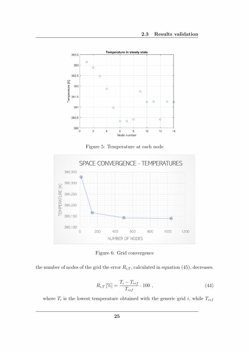
2.3.2 Temperatures
With a network of 14 nodes the temperature obtained at each node are the ones
illustrated in figure 5.
This plot shows how the temperature drops from the inlet point until the furthest
node. In order to validate these results a space convergence has been performed:
increasing the number of nodes for the same district heating network (in figure 4).
The error with respect to the more refined grid is decreasing proportionally with
the number of nodes, as the convergence should be. Table 3 shows how increasing
24
2.3 Results validation
Figure 5: Temperature at each node
Figure 6: Grid convergence
the number of nodes of the grid the error Ri,T , calculated in equation (45), decreases.
Ri,T [%] =Ti − TrefTref
· 100 , (44)
where Ti is the lowest temperature obtained with the generic grid i, while Tref
25

2.3 Results validation
is the lowest temperature obtained with the more refined grid.
Table 3: Error of the 3 grids with respect to the more refined one
Number of nodes Error [%]14 0,0479140 0,0067500 0,0005
On the contrary, in the case of unsteady state condition, the refinement of the
grid is more crucial in order to obtain an accurate result. As shown in figure 7,
the behaviour of temperature in time (the furthest node has been considered) is
described in a different manner according to the grid used. In fact, in a district
heating network, the temperature increases in a limited amount of time: at the
beginning of the simulation it remains stable, until the hot fluid reaches the node
taken into consideration, and then the node reaches in short time the steady state
temperature [13]. Obviously, the more refined is the grid the more precise will be
the time interval in which the change of temperature occurs. Moreover, you see how
the different behaviour between a grid with tens of nodes and a grid with hundreds
of nodes is far more remarkable than the different behaviour observed between the
two grid with hundreds and thousands number of nodes.
Figure 7: Temperature of the last node in time with three different grid refinements
26
2.3 Results validation
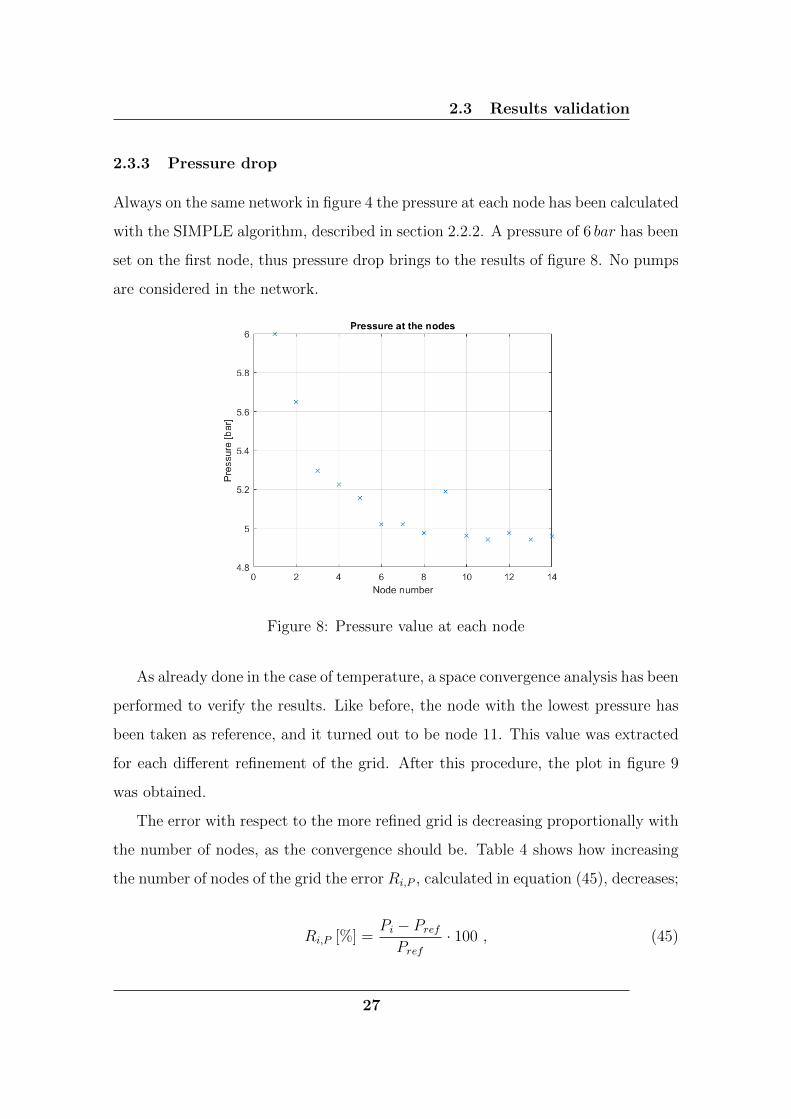
2.3.3 Pressure drop
Always on the same network in figure 4 the pressure at each node has been calculated
with the SIMPLE algorithm, described in section 2.2.2. A pressure of 6 bar has been
set on the first node, thus pressure drop brings to the results of figure 8. No pumps
are considered in the network.
Figure 8: Pressure value at each node
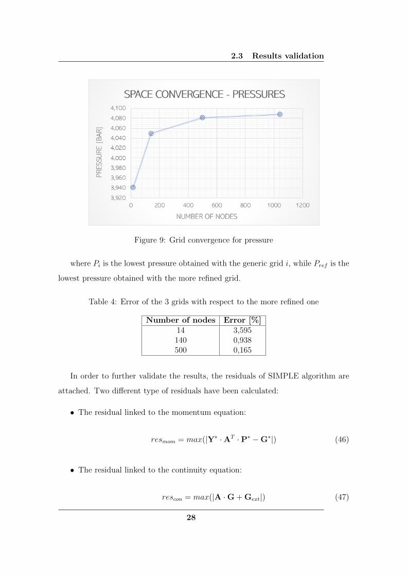
As already done in the case of temperature, a space convergence analysis has been
performed to verify the results. Like before, the node with the lowest pressure has
been taken as reference, and it turned out to be node 11. This value was extracted
for each different refinement of the grid. After this procedure, the plot in figure 9
was obtained.
The error with respect to the more refined grid is decreasing proportionally with
the number of nodes, as the convergence should be. Table 4 shows how increasing
the number of nodes of the grid the error Ri,P , calculated in equation (45), decreases;
Ri,P [%] =Pi − Pref
Pref
· 100 , (45)
27
2.3 Results validation
Figure 9: Grid convergence for pressure
where Pi is the lowest pressure obtained with the generic grid i, while Pref is the
lowest pressure obtained with the more refined grid.
Table 4: Error of the 3 grids with respect to the more refined one
Number of nodes Error [%]14 3,595140 0,938500 0,165
In order to further validate the results, the residuals of SIMPLE algorithm are
attached. Two different type of residuals have been calculated:
• The residual linked to the momentum equation:
resmom = max(|Y∗ ·AT ·P∗ −G∗|) (46)
• The residual linked to the continuity equation:
rescon = max(|A ·G + Gext|) (47)
28

2.3 Results validation
For each iteration of the SIMPLE algorithm these two operations have been per-
formed such that the following plots are obtained:
Figure 10: Residual linked to the momentum equation
Figure 11: Residual linked to the continuity equation
It can be noticed how both of the residuals converge after about 10-20 iterations
of the SIMPLE algorithm, and the higher of the two (rescon) reaches the tolerance
29

2.3 Results validation
imposed (10−5) after about 40 iterations.
As a matter of fact, since the network taken into consideration has no loops,
the mass flow rate is known and consequently also the vector of the pressures can
be calculated explicitly with equation (19). The calculation brings to the results in
figure 12.
Figure 12: Pressure calculated with momentum equation, without SIMPLE
Thus it is possible to compare these results with the values obtained with SIM-
PLE algorithm. As table 5 shows, the maximum error occurs in the most distant
node and it is around 2%. In practical terms there is a difference between the two
models of about 0,025 bar/km.
As final comments, there results are considered satisfactory in order to further
analyze the data.
In post-processing some sensitivity analyses will be performed in order to study the
fluid-dynamic response of the district heating network to the change of some inputs.
Another important parameter that will be fundamental in the final part of the work
are heat losses, that in the next section will be mathematically treated.
Moreover the return line behaviour will be simulated and studied, modelling the
30

2.3 Results validation
Table 5: Percentage error of pressure obtained with SIMPLE with respect to pressureobtained with equation (19)
Node Error [%]1 02 0,5783 1,2604 1,4115 1,5686 1,7697 1,9198 1,8449 1,4931 1,83911 1,87012 2,04913 2,15414 2,099
system according to the real design of actual technologies, that can be found in
district heating network spread all over the world.
31

3 Analysis on the network
3 Analysis on the network
3.1 Return network
In order to study the system completely, a model of return network is needed. The
work above depicted is useful to simulate the temperature of the transfer fluid that
arrives at the users (Tout,s). At this point the water enters in the heat exchanger in
order to provide the requested thermal load to the users, as described in figure 13.
At this point, in order to calculate the inlet temperature of return line (Tin,r) it is
necessary to refer to the users heat demand listed in table 1 and, for each user node,
the following formula is applied:
Tin,r = Tout,s −Φ
|Gcp|(48)
Figure 13: Heat exchanger from district heating to the users [14]
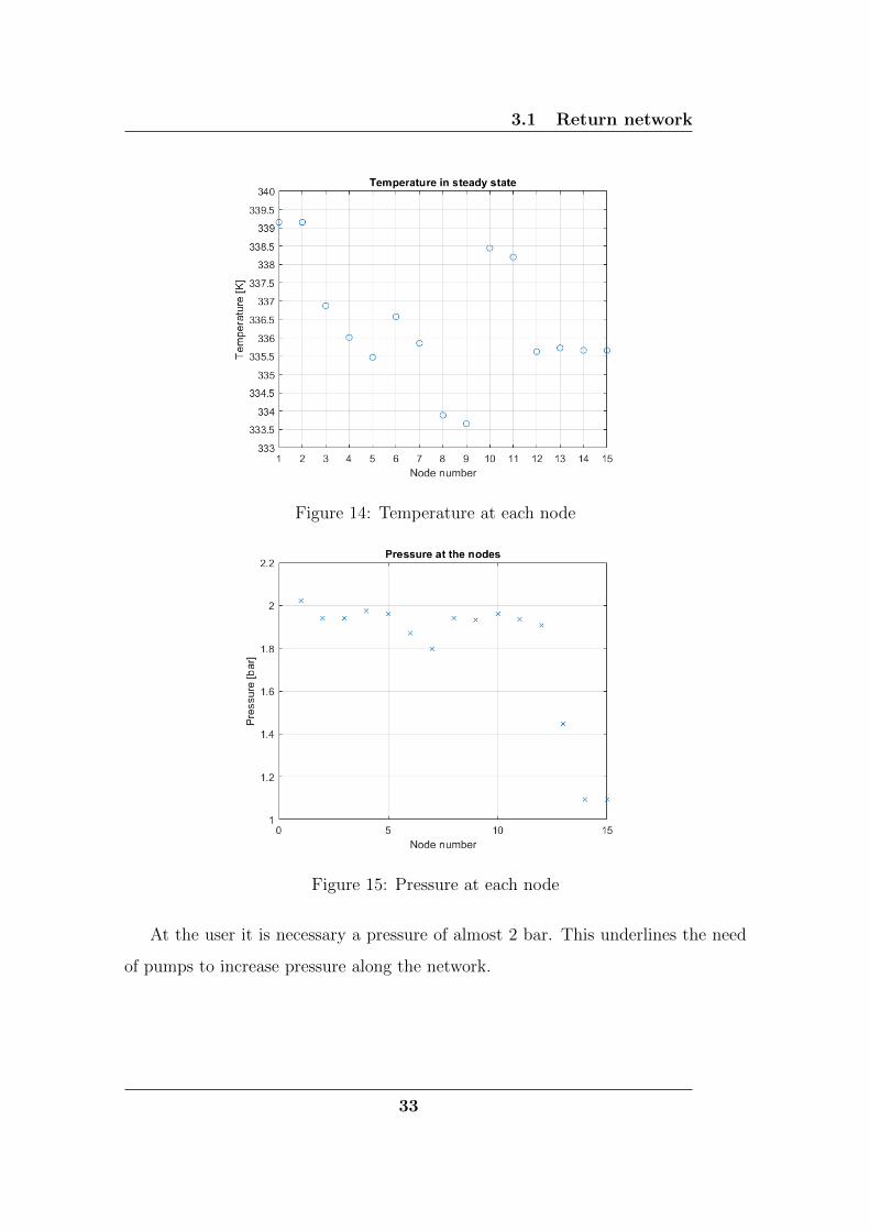
The temperatures obtained are presented in figure 14. The return temperature
is about 60◦C.
The pressure calculation has been performed with a minimum pressure drop
available at the user equal to 2 bar. In this way, in order to obtain the inlet pressure
of the return network you just need to subtract the minimum pressure drop available
at the user to the outlet pressure of the supply network. The results are in figure
15.
32
3.1 Return network
Figure 14: Temperature at each node
Figure 15: Pressure at each node
At the user it is necessary a pressure of almost 2 bar. This underlines the need
of pumps to increase pressure along the network.
33

3.2 Load variation analysis
3.2 Load variation analysis
In order to study the behaviour of the system in case of load variation, a variation of
heat demand by the users has been assumed. This causes, as explained in equation
(43), a change of mass flow rate, since specific heat and temperature difference are
constant.
In the following plot the data of table 1 have been scaled according to a certain
factor (1,25; 1,5; 2), and the temperatures have been calculated again.
Figure 16: Temperature profile at each node with different heat demand
It can be noticed how, with an increase of heat demand the temperatures are
higher. This is because an increase of mass flow rate, being the diameter constant,
means an increase of velocity. In this way the hot fluid takes less time to arrive to
the users, so it has less time to lose its heat. In simple terms, an increase of thermal
inertia occurs.
Obviously the pressure drops will be higher, due to the higher mass flow rate: pres-
sure drops are proportional to the square of velocity.
34

3.3 Heat Losses
Figure 17: Variation of pressures with the load
3.3 Heat Losses
An analysis of the heat losses in this network taken as example is performed. The
value of the heat losses is obtained for generic branch j from the formula, with
reference to figure 3.
Φd,j =
nrami∑j=1
LjIjUj · (Tj − Tg) (49)
where Tj =Ti + Ti−1
2. This operation is performed for each branch, in this way a
profile of heat losses along the network is produced.
3.3.1 Heat losses in steady state
The heat losses are considered in Watt, this means that the value of the losses
are intended as power lost per second. In the case of temperatures calculated in
steady state, in order to calculate the heat losses over a period of time, is obviously
necessary to multiply the value in Watt by the time that composes that period.
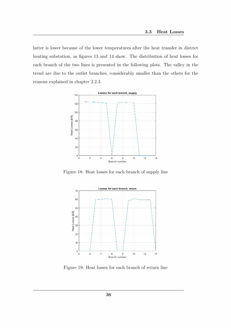
The code tells us that the values of heat losses in steady state condition are
0, 806MW for the supply line and 0, 33MW for the return line. Obviously the
35
3.3 Heat Losses
latter is lower because of the lower temperatures after the heat transfer in district
heating substation, as figures 13 and 14 show. The distribution of heat losses for
each branch of the two lines is presented in the following plots. The valley in the
trend are due to the outlet branches, considerably smaller than the others for the
reasons explained in chapter 2.2.3.
Figure 18: Heat losses for each branch of supply line
Figure 19: Heat losses for each branch of return line
36

3.3 Heat Losses
3.3.2 Heat losses in transient condition
In order to calculate the heat losses while the system is switching on or off, it is
necessary to calculate the losses with the temperatures obtained in every time step
of unsteady state condition. The sum of them is the total losses during the transient
operation.
The trend is expected to be increasing with time, since the temperatures of the
network increase with time thanks to the incoming hot fluid. Moreover the trend is
not linear because, as figure 7 shows, the temperature at a generic node does not
increase linearly.
Figure 20: Heat losses in time of supply line
As it can be seen both the transient start after the first time step with a value
of losses that is almost equal between the two, since at time 0 they are the same
network at the same temperature. After the transient has finished, the final value
is equal to the one calculated in steady state condition.
It is possible to notice that the return curve has an almost linear behaviour at
first time, this is due to the initial temperature which is really close to ground
temperature, and so the increasing trend is faster and almost linear.
37

3.3 Heat Losses
Figure 21: Heat losses in time of return line
3.3.3 Sensitivity analysis with ground temperature
Heat losses will be an important parameter to evaluate the systems in next chapters,
for this reason a further confirmation of the results is deemed to be necessary.
Figure 22: Heat losses dependent on ground temperature
As equation (49) shows, being constant the coefficients, the value of heat losses
38

3.3 Heat Losses
are linearly proportional to ground temperature: the more it is higher, the lower will
be the dissipation of heat toward the environment. The plot in figure 22 corroborates
this analysis.
39

4 Case study: introduction of district heating in a gas network
4 Case study: introduction of district heating in
a gas network
In order to apply the model constructed and described in the previous chapter, a
substitution of natural gas users with district heating users in a industrial and urban
area is taken into consideration.
4.1 Urban area description
The urban area concerned is described in the figure 23.
Figure 23: Urban area topology
The unit cell dimension is 100 x 100 m, while the entire square is 4.4 x 5 km.
Different colours correspond to different kind of users:
• Green: RESIDENTIAL user. Different shade: low-medium-high density (from
light to dark).
• Yellow: COMMERCIAL user. Different shade: electricity meter allowed power
(6, 10, 15, 20 and 30 kW from light to dark).
40

4.1 Urban area description
• Pink: OFFICES. Different shade: electricity meter allowed power (3, 6 and 9
kW from light to dark).
• Red: INDUSTRIAL user.
As far as the natural gas flow rate is concerned, the figure 24 describes the area.
Figure 24: Natural gas volumetric flow rate
Each zone is fed by second jump reduction group in which the pressure drops
down, so that it can supply a low pressure network until the gas meter of each user.
The area coloured in dark red are industrial area directly fed by medium pressure
network. The other colours identify the maximum hourly volumetric flow rate of
natural gas, according to the legend of figure 25.
Figure 25: Legend of natural gas flow rate
41

4.1 Urban area description
For the sake of clarity, the following table shows the consumption of natural gas
for each node.
Figure 26: Natural gas consumption for each node
Before moving to the system sizing, a specification is necessary. What in figures
23 and 24 is represented as a node, is not a single user but a group of users. The
figure 27 sums up the topology in detail.
Figure 27: Users of the network
42

4.2 Consumption profiling
4.2 Consumption profiling
4.2.1 Daily consumption
In figure 26 are listed the users heat demands for each node of the network. Before
starting with the simulation it is necessary to translate the total annual consumption
in hourly consumption, in order to obtain the water mass flow rate needed as an
input of the Matlab code.
In order to do this, an important document of the natural gas authority comes
into help [27]. In this document (Section 2, Article 5 and 6) the profiling procedure
is described. It consists in taking the annual value and multiplying it by the daily
percentage value p%PROF,k. This parameter is different for each day of the year, and
it allows to obtain, from the annual consumption, a value of consumption for each
day of the year. The calculation is based on other parameters that change according
to the season, the month and even the day of the week:
p%PROF,k = Wkr · β1PROF · c1%
i,j,k + β2PROF · c2%k + β3PROF · 1%
j,k + β4PROF · c4%k (50)
where:
• i is the climatic zone (A, B, C, D, E, F)
E class is chosen, which is the zone of Pianura Padana (including Torino) and
central Italy mountains, as shown in figure 28 and 29.
• j is the picking class, defined in table 6.
Table 6: Picking class from arera [27]
CODE PICKING CLASS1 7 days2 6 days (Sunday and festivities excluded)3 5 days (Saturday, Sunday and festivities excluded)
In this study class 1 has been chosen for industrial and residential users, while
43

4.2 Consumption profiling
Figure 28: Climate zone in Italy
Figure 29: Legend of climate zone in Italy and corresponding Degree Day values
class 3 for offices and commercial users.
• c1%i,j,k is the percentage value in the day k of standard picking connected to
the gas used for heating purposes, in climate zone i and for picking class j.
• c2%k is the percentage value in day k of standard picking connected to food
cooking and/or sanitary hot water.
• t1%j,k is the percentage value, at day k, of standard picking connected to tech-
nological use of natural gas and picking class j.
• c4%k is the percentage value in day k of standard picking connected to the is
of gas for conditioning.
44
4.2 Consumption profiling
• β1PROF , β2PROF , β3PROF , β4PROF are coefficients, defined in table 7, that
identify the category of use of gas.
• Wkr is a climate correction factor associated to day k and climate region r.
All these values are published in the website of the company that is Balance
Responsible (the bigger distribution company).
For this study, category C3 is chosen (heating + cooking and/or production of
sanitary hot water). In order not to consider the cooking gas demand in the total
demand that district heating must supply, the consumption of residential users has
been decreased of a 5%.
Table 7: Gas category of use [27]
CODE DESCRIPTIONC1 7 HeatingC2 Cooking and/or hot water productionC3 Heating + cooking and/or hot water productionC4 ConditioningC5 Conditioning + heatingT1 Technological useT2 Technological use + heating
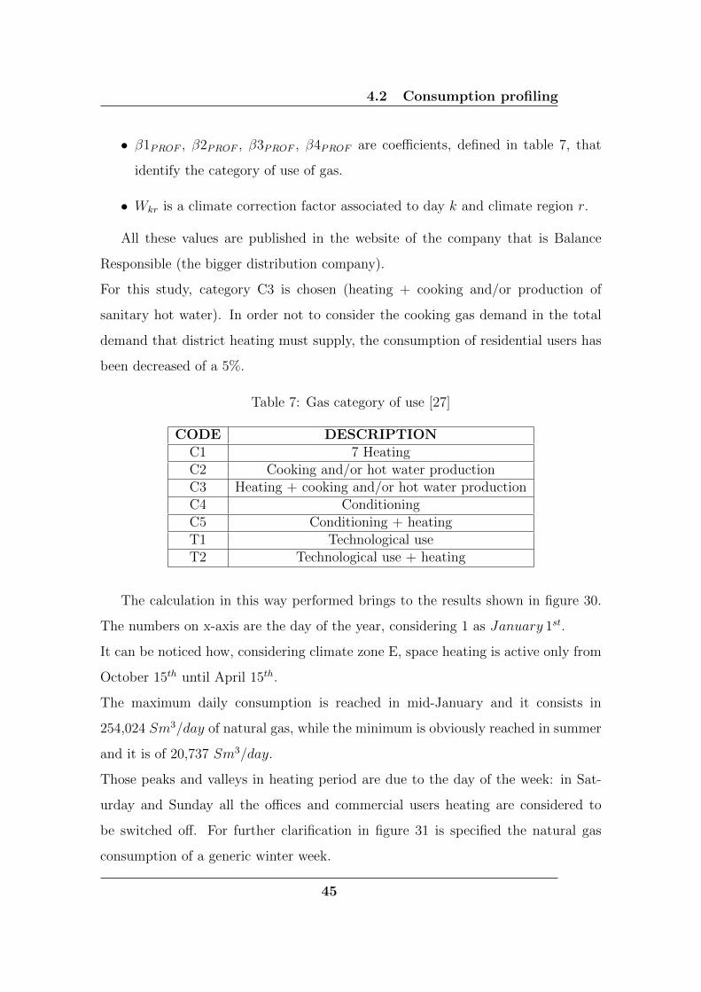
The calculation in this way performed brings to the results shown in figure 30.
The numbers on x-axis are the day of the year, considering 1 as January 1st.
It can be noticed how, considering climate zone E, space heating is active only from
October 15th until April 15th.
The maximum daily consumption is reached in mid-January and it consists in
254,024 Sm3/day of natural gas, while the minimum is obviously reached in summer
and it is of 20,737 Sm3/day.
Those peaks and valleys in heating period are due to the day of the week: in Sat-
urday and Sunday all the offices and commercial users heating are considered to
be switched off. For further clarification in figure 31 is specified the natural gas
consumption of a generic winter week.
45

4.2 Consumption profiling
Figure 30: Total annual consumption of the users
Figure 31: Weekly consumption of the users
4.2.2 Hourly profiling
Now from the daily consumption it is necessary to obtain an hourly profile in order
to give the input at the Matlab Code.
The method used is a simple multiplication of the daily value by a percentage p%
that is taken from the figure 32 and that changes according to the time of the day.
From the plots is clear how the residential users and offices have a very low
consumption during night, while industries and commercial users have a remarkable
activity also during the night.
46

4.2 Consumption profiling
Figure 32: Hourly consumption percentage with respect to total daily consumption
4.2.3 Calculation of thermal demand and mass flow rate
The last step before running the code is calculate the hourly mass flow rate. In
order to do that it is necessary to know the heat demand of each user.
The starting point is the natural gas consumption qNG. Imposing a Low Heating
Value of natural gas LHVNG of 35.046MJ
Sm3[25] and a nominal temperature drop
between the supply and the return line of DHN:
∆Tnom = (129◦C − 65◦C) = 55◦C (51)
it is possible to calculate the thermal power demand from the natural gas consump-
tion qNG:
Φ[W ] = qNG · LHVNG · ηth , (52)
after that, considering the definition of heat demand:
47

4.2 Consumption profiling
Φ = G · cp,water ·∆T (53)
from equations (52) and (53) it is possible to calculate the mass flow rate profile for
each node:
G =qNG · LHVNG · ηth
G · cp,water
(54)
At this point all the values needed are known, except for the thermal efficiency
of the natural gas boilers. For the estimation of it an important document pub-
lished by Piemonte comes into help [28]. In the Annex there is the method for the
calculation of the minimum combustion efficiency allowed, measured at maximum
effective thermal power in condition of normal operation, resulting in the following
expression:
ηc [%] = 0.9 · [93 + 2 · log(Pn)] (55)
where log(Pn) to base 10 of useful nominal thermal power of the generator. For
values Pn > 400 kW , the maximum limit of 400 kW is applied.
Since these are the minimum values that the Authority impose to reach within
September 2020, a 90% of this value is supposed.
In the case of this work the efficiency obtained in this way vary from 0.87 and
0.88.
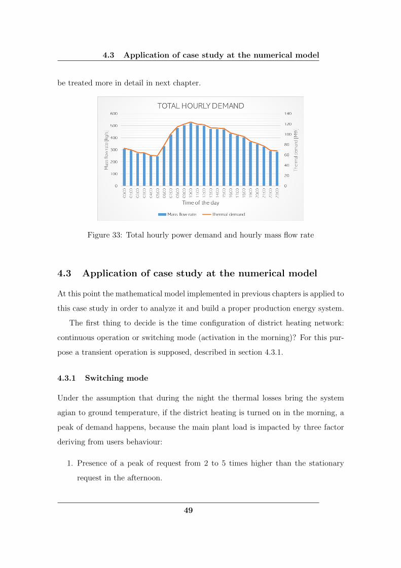
This method allows to calculate also the hourly profile of thermal demand and
consequently mass flow rate. The results for node 1 (which means the total of the
system) are shown in figure 33, taking into consideration a generic day of February
(near the maximum power demand).
It is possible to notice that during the night the demand is not negligible, and it is
not less than one half of the peak demand. This leads to think that switching off
the district heating during night is not feasible and convenient, but this topic will
48
4.3 Application of case study at the numerical model
be treated more in detail in next chapter.
Figure 33: Total hourly power demand and hourly mass flow rate
4.3 Application of case study at the numerical model
At this point the mathematical model implemented in previous chapters is applied to
this case study in order to analyze it and build a proper production energy system.
The first thing to decide is the time configuration of district heating network:
continuous operation or switching mode (activation in the morning)? For this pur-
pose a transient operation is supposed, described in section 4.3.1.
4.3.1 Switching mode
Under the assumption that during the night the thermal losses bring the system
agian to ground temperature, if the district heating is turned on in the morning, a
peak of demand happens, because the main plant load is impacted by three factor
deriving from users behaviour:
1. Presence of a peak of request from 2 to 5 times higher than the stationary
request in the afternoon.
49

4.3 Application of case study at the numerical model
2. Peak of request strengthened by the fact that the thermal load must heat up
at the operating temperature a network that is all at ground temperature.
3. Demand variation is linked to a mass flow rate variation that has an immediate
effect on plants thermal load (delay of about 0.5 s/km, because fluid-dynamic
perturbations travel with sound speed).
4. Request variation is connected to a return temperature variation that has a
delayed effect on plant load (considering mean velocity of 1 m/s, the delay is
around 15 min/km.
For all these reasons an example of plant thermal load is like the one presented in
figure 34. Obviously the values are much higher than the ones treated in this case
study because the plot refers to the entire city of Turin.
Figure 34: Total plant load in Turin [29]
With the aim of simulating this situation, a guess has been made. There are two
ways for simulate the heat demand variation of the user:
1. Primary net mass flow rate variation;
50
4.3 Application of case study at the numerical model
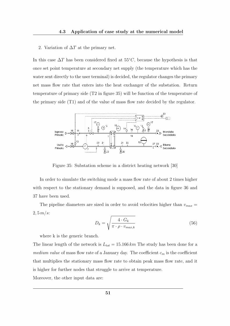
2. Variation of ∆T at the primary net.
In this case ∆T has been considered fixed at 55◦C, because the hypothesis is that
once set point temperature at secondary net supply (the temperature which has the
water sent directly to the user terminal) is decided, the regulator changes the primary
net mass flow rate that enters into the heat exchanger of the substation. Return
temperature of primary side (T2 in figure 35) will be function of the temperature of
the primary side (T1) and of the value of mass flow rate decided by the regulator.
Figure 35: Substation scheme in a district heating network [30]
In order to simulate the switching mode a mass flow rate of about 2 times higher
with respect to the stationary demand is supposed, and the data in figure 36 and
37 have been used.
The pipeline diameters are sized in order to avoid velocities higher than vmax =
2, 5m/s:
Dk =
√4 ·Gk
π · ρ · vmax,k
(56)
where k is the generic branch.
The linear length of the network is Ltot = 15.166 km The study has been done for a
medium value of mass flow rate of a January day. The coefficient cm is the coefficient
that multiplies the stationary mass flow rate to obtain peak mass flow rate, and it
is higher for further nodes that struggle to arrive at temperature.
Moreover, the other input data are:
51

4.3 Application of case study at the numerical model
Figure 36: Diameters and length of pipelines
Figure 37: Mass flow rate for each node, with peak mass flow rate
• Roughness ε=0.003 mm
• Heat transfer coefficient of the pipes toward the ground h=1.2W
m ·K
• Specific eat of water cp = 4186J
kg ·K
52

4.3 Application of case study at the numerical model
• Ground temperature Tg = (120 + 273.15)K
• Mean water density ρwater = 970kg
m3
• Friction factor λj calculated like in section 2.2.1.
With all these input data the code can run. The first results are velocities and
pressures.
Figure 38: Pressure and velocity of switching mode
The velocity values are stopped at 2.5 m/s, as already explained, while the
maximum pressure drop (in supply side) is 1.512 bar, that is a high but affordable
value, since the pumping system load would be:
tPUMP = ∆Pmax + Pmin + Luser = 5.512 bar (57)
where Pmin is the minimum return pressure to the plant (2 bar) and Luser is the
pressure drop at the user, supposed to be 2 bar.
As far as heat losses are concerned, both for supply and return line, figure 39
shows as they rapidly increase when the network is near the ground temperature,
while it reaches a plateau after about 2 hours.
The thermal power peak, instead, is visible in figure 40, due to the reasons
already explained in the previous paragraph.
53

4.3 Application of case study at the numerical model
Figure 39: Heat losses in time for supply and return line
Figure 40: Thermal power in time provided to the network
The real problem of this configuration, though, are the temperature reached in
time. In fact, starting from ground temperature in the morning the system must
be capable of bringing all the users at the stationary temperature in a proper time.
This proper time is supposed equal to 2 hours. But after 2 hours the situation is
the one described in figure 41.
The blue line identify the stationary temperature (with a tolerance), and it is
possible to notice that not all the nodes have reached that value. In particular, all
the users at nodes 11, 26, 34, 37, 68, 70, 73, 77 and 78 have a temperature too low
for the correct operations of the substation heat exchanger. Moreover, it would be
infeasible to increase velocities, because they are already at the maximum limit, and
pressure losses would be too high.
For a better comprehension, the figure 42 shows the graph representation of
54

4.3 Application of case study at the numerical model
Figure 41: Temperature at the nodes after 2 hours from the switching
the temperature after 2 hours. It can be seen how the furthest node are not in
temperature.
Figure 42: Temperature at the nodes after 2 hours from the switching on
It follows that the switching mode is not the best option in this case, also because
the consumption at night is not negligible and it justifies a continuous operation
mode for district heating network.
55

4.3 Application of case study at the numerical model
4.3.2 Continuous operation mode
At this point the continuous operation mode is simulated.
In order to do that, from the calculation of hourly consumption the hourly mass
flow rate is extracted for each node. The transient model has been performed with
a time step of 100 seconds: the value of mass flow rate available has a discretization
of 1 hour, so in order to transform the 1 hour step in a 1000 seconds step a linear
variation of mass flow rate is supposed. With interpolation the input values for the
code every 100 seconds are obtained.
By way of illustration, the steady state temperature for supply and return line,
in the case of maximum mass flow rate reached in January are showed in figure 43.
Figure 43: Temperature in steady state of supply and return line
For a better comprehension of the situation in the network, the figures 44 and 45
are proposed, that depict the temperature and velocities of the line. The coloured
walls of the branches are referred to the legend at the left of the figure, while the
colour in the center of the branches is referred to the legend at the bottom, showing
temperature.
Here it is clear how the temperature has a descending trend, more and more as
we are far from the feed of the hot water. The velocities instead do not have an
organised trend, because they depend on the mass flow rates that are lower so as
they are far from the injection, but also on diameters.
56

4.3 Application of case study at the numerical model
Figure 44: Temperature in steady state and velocities of supply line
Figure 45: Temperature in steady state of return line
The temperature decreases of about 4.5◦C. The return line has less ”organized”
temperature because the mass flow rate has inverted sign, so there is not separation
of the flows but mixing of the flows. As a matter of fact it can be noticed how one
the furthest node of return (node 1) the temperature is higher than the temperature
of some nodes that are at the beginning of this return line, near the users.
57

4.3 Application of case study at the numerical model
Always by way of illustration figure 46 describe the heat losses for each branch. It
is possible to notice how branch 37 is the longer one of the network, and consequently
it dissipates the higher amount of thermal power to the environment. Obviously the
return line heat losses are way lower because of lower operating temperature.
Figure 46: Heat losses of each branch at steady state for supply and return line
Figure 47: Heat losses for each branch
Also here the pattern does not have a relevant and significant order, it depends
specially on the length of the branch.
Turning now to transient real model, the mass flow rate variation brings a pres-
sure variation and a temperature variation during the day, according to the thermal
58

4.3 Application of case study at the numerical model
demand that users require. Two examples of industrial and non industrial node are
provided. The profile of return line is equal but about 55◦C lower.
The temperature profile follows the heat demand profile: for a higher thermal power
required there is a higher mass flow rate, that means a lower thermal inertia so the
hot water at 120◦C is more easily transferred with less thermal losses, as already
explained in figure 16.
Figure 48: Mass flow rate and temperature in a day of January for a non industrialnode
Figure 49: Mass flow rate and temperature in a day of January for an industrialnode
As far as pressure losses are concerned, in a generic day of January they vary with
the heat demand. The variation of mass flow rate strongly influences the pressure
losses, that are quadratically proportional to the velocity. The pressure profile at
maximum and minimum load is presented in figure 50.
59

4.3 Application of case study at the numerical model
The ∆pmax in the total line is of 1.616 bar, but the difference with respect to the
minimum mass flow rate configuration is remarkable: in this case the maximum
pressure loss in the line is about 0.4 bar.
Figure 50: Maximum and minimum pressure profile in a day of January
In figure 51 is described the variation of pressure along the line: the values are
obtained imposing a value of return in the plant of 2 bar, and a pressure drop at
the user of 2 bar, too. So the total pumping system load can be calculated:
tPUMP = 7.2− 2 = 5.2 bar (58)
In figure 52 is represented the supply line with its pressures along the pipes, and
here is highlighted the pressure drop at the user, the return pressure to the plant
and the total pump load.
Now the analysis moves on one of the most important parameter of the study:
the amount of thermal losses. During the day they follow the temperature profile,
as can be imagined, and in the usual case of a generic January day shows up like
in figure 53. This is because the ground temperature is supposed constant during
the day, so the only parameter that changes during the day is the the network
temperature. Thus the profiles are perfectly comparable. However the variations
60

4.3 Application of case study at the numerical model
Figure 51: Pressure along the network
Figure 52: Pressure along the supply line
are limited.
Before turning to the annual analysis, the power profile and the percentage of
losses with respect to thermal power are shown.
Finally also the residuals of SIMPLE algorithm are presented, in order to validate
the results.
61

4.3 Application of case study at the numerical model
Figure 53: Daily profile of thermal losses
Figure 54: Daily profile of thermal power and percentage of losses
Figure 55: SIMPLE algorithm residuals
62

4.3 Application of case study at the numerical model
4.3.3 Annual results analysis
Once the daily behaviour of the system is described, it is necessary to analyze the
system behaviour over an entire year, and then choose the best options for providing
energy to the system studied.
The annual behaviour is studied by simulating every single day of the year with
its own input data calculated in previous chapters. After that, all the data was
collected and plotted in the following figures.
Figure 56: Pressure drop on supply line every day of the year
As already said, pressure drops are strongly dependent on mass flow rate. In
summer the heat demand is very low, so it is mass flow rate and so are the pressure
losses. From this the trend in figure 56.
In figure 57 is shown as the energy provided to the system in summer decreases
a lot more than the thermal losses, because while the thermal request drops signifi-
cantly, the temperature does not do the same, decreasing only of a few degrees.
This brings to the results shown in figure 58, that shows how the percentage,
calculated on energy, varies from 2% in winter to 15% in summer, with an annual
mean of 8.97%. The same percentage calculated instead om power, is about 2-3%
because it is not affected by the high summer percentage weight.
63

4.4 Production energy system design
Figure 57: Energy provided to the system and total thermal losses along the year
Figure 58: Total thermal losses along the year with correspondent percentage onthe total energy provided
4.4 Production energy system design
At this time every detail of energy demand is known and calculated. For the purpose
of this study two configurations of energy production are treated:
1. CASE 1: CENTRALIZED GENERATION
In this case a single big plant, with an auxiliary boiler for peak demand is
located in node 1. It is a centralized energy production configuration, in
which all the thermal energy needed is produces in a single plant, and the hot
water is heated up from the final return temperature to the supply temperature
64

4.4 Production energy system design
(120◦C).
2. CASE 2: DISTRIBUTED GENERATION
In this case the big plant power is reduced and supply temperature is decreased
to 90◦C, trying to reduce thermal losses. This means that in order to reach
the supply temperature at which the substations are designed to work there
is the need of some thermal boosters that, near the users node, heats up the
water to the requested temperature.
The choice of the type of energy production plants is the next step of the study.
The possibilities for a district heating network with this kind of thermal demand
are:
• Small (case 2) or medium (case 1) size cogeneration plants;
• WTE systems;
• Waste heat form industrial processes;
• Biomass boilers;
• Heat pumps (case 2);
• Solar collectors (in case 2).
The choice in this basic analysis is the first possibility of the four: it is the most
used and the best one in order to analyze all the project also under an economic
point of view. Moreover, the connection with electricity grid and gas network may
open the doors for further and more detailed studies on energy networks.
4.4.1 Combined heat and power (CHP) technologies
The Combined Heat and Power energy production consists in the combined produc-
tion of two different forms of energy with a single conversion process. Usually these
forms of energy are electrical energy and thermal (heating or cooling) energy.
65

4.4 Production energy system design
Figure 59: CHP production operating principle
The ratio between thermal and electrical energy produced is an important index
in CHP production, and is strongly dependent on the technology used, as the table
8 of ARERA shows [22];
Table 8: Energy/Heat ratio for different CHP technologies
TECHNOLOGY ENERGY/HEAT RATIOCombined Cycle 0.95
Back pressure steam turbine 0.45Condensation steam turbine 0.45
Gas turbine with heat recovery 0.55Internal combustion engine 0.75
Some important parameters for cogeneration plants are the efficiencies:
ηel =Eel
Ef
(59)
ηth =Eth
Ef
(60)
ηtot =Eel + Eth
Ef
(61)
where Eel is the total amount of electrical energy produced, Eth the total thermal
energy produced and Ef the primary energy consumption (fuel).
Another important index is the Primary Energy Saving, that identifies how much
primary energy has been saved by producing energy in cogeneration configuration
66

4.4 Production energy system design
instead of traditional one.
PES = 1− 1Eth
ηth,trad · Ec
+Eel
ηel,trad
(62)
where ηtrad is the efficiency of traditional energy production plants.
The most important advantages of cogeneration are the reduction of primary
energy demand, due to the utilization of thermal energy that is usually dissipated in
the environment and the lower electrical losses of transportation and distribution.
Moreover this technology allows a reduction of environmental impact and a general
saving for the purchase of energy.
The most relevant technologies for CHP production are:
• INTERNAL COMBUSTION ENGINES
The advantages of this technologies are the big commercial availability (from
some kW to 20 MW); the high electrical efficiency, until 45%; a good behaviour
at partial loads, a high energy/heat ratio.
But there are some fundamental problems for the use of this technology in this
work. The first one is technical: these boosters have to heat up the water from
90◦C to 120◦C, while the ICEs make available thermal heat until 95◦C, which
is a too low value. The higher emissions and high maintenance cost exclude
this technology from this study.
Figure 60: An internal combustion engine
These technology has one degree of freedom: available thermal power is uni-
vocally connected to electrical power. This means that a partial engine load,
67

4.4 Production energy system design
both of energy fluxes decrease. This can be a problem in summer when the
thermal energy needed by the district heating network is low, and it would be
better to produce a high amount of electricity with a low heat production, in
order to send more eletrical energy.
• GAS TURBINE
Also this technology disposes of a high commercial availability, from micro-
turbines of 30 kWe until big system of above 250 MWe. Moreover the GT
are widely used and affordable, and the waste heat is at a high temperature
(500◦C). Also the costs are quite low.
The drawbacks are the impossibility of intermittent operation and low electri-
cal efficiency until medium size plants. In addition they have a low electric-
ity/heat ratio.
But for the purpose of this study they are the best option thanks to the mod-
ularity and the availability of high temperature heat.
Figure 61: A gas turbine
• OTHER TECHNOLOGIES
An other important technology is steam turbine, but they are massive systems
with extremely low electrical efficiency and energy/heat ratio.
Other technologies under development are Fuel Cell and Heat Pumps, with an
interesting future also under the point of view of environment protection.
68

4.4 Production energy system design
Figure 62: CHP technologies in function of available sizes and electrical efficiency[31]
4.4.2 Case 1: centralized generation
Thanks to the Matlab model it is possible to build the cumulative curve of thermal
demand. The power calculated every hour is sorted in descending order and the
figure 63 is obtained.
Figure 63: Cumulative curve of thermal demand
The best configuration in this case is a CHP plant based on a gas turbine of
90MWth and a coupling of electrical and thermal energy of this type: the cogen-
eration plant follows the user thermal profile, producing in each instant the energy
power requested, and the electrical energy consequently produced is sold to the grid.
The configuration of the plant is described in figure 64.
69
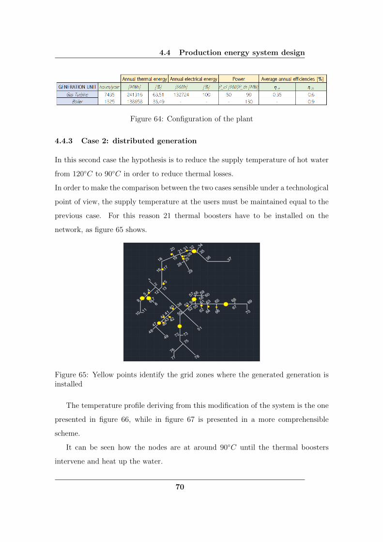
4.4 Production energy system design
Figure 64: Configuration of the plant
4.4.3 Case 2: distributed generation
In this second case the hypothesis is to reduce the supply temperature of hot water
from 120◦C to 90◦C in order to reduce thermal losses.
In order to make the comparison between the two cases sensible under a technological
point of view, the supply temperature at the users must be maintained equal to the
previous case. For this reason 21 thermal boosters have to be installed on the
network, as figure 65 shows.
Figure 65: Yellow points identify the grid zones where the generated generation isinstalled
The temperature profile deriving from this modification of the system is the one
presented in figure 66, while in figure 67 is presented in a more comprehensible
scheme.
It can be seen how the nodes are at around 90◦C until the thermal boosters
intervene and heat up the water.
70

4.4 Production energy system design
Figure 66: Temperature profile of supply line in case 2
Figure 67: Temperature of supply line in case 2
Figure 68 shows, instead, how the thermal losses in configuration 2 are decreased
of about 20% and the mean percentage on the total energy provided is down to 8.4%
from the previous 9%.
With the same method of centralized distribution, the cumulative curves of these
21 boosters are calculated and presented in the following figures (example of node
1, the power plant, and an industrial and non industrial node.
This allows to half the thermal power of cogeneration plant, whose data are
71
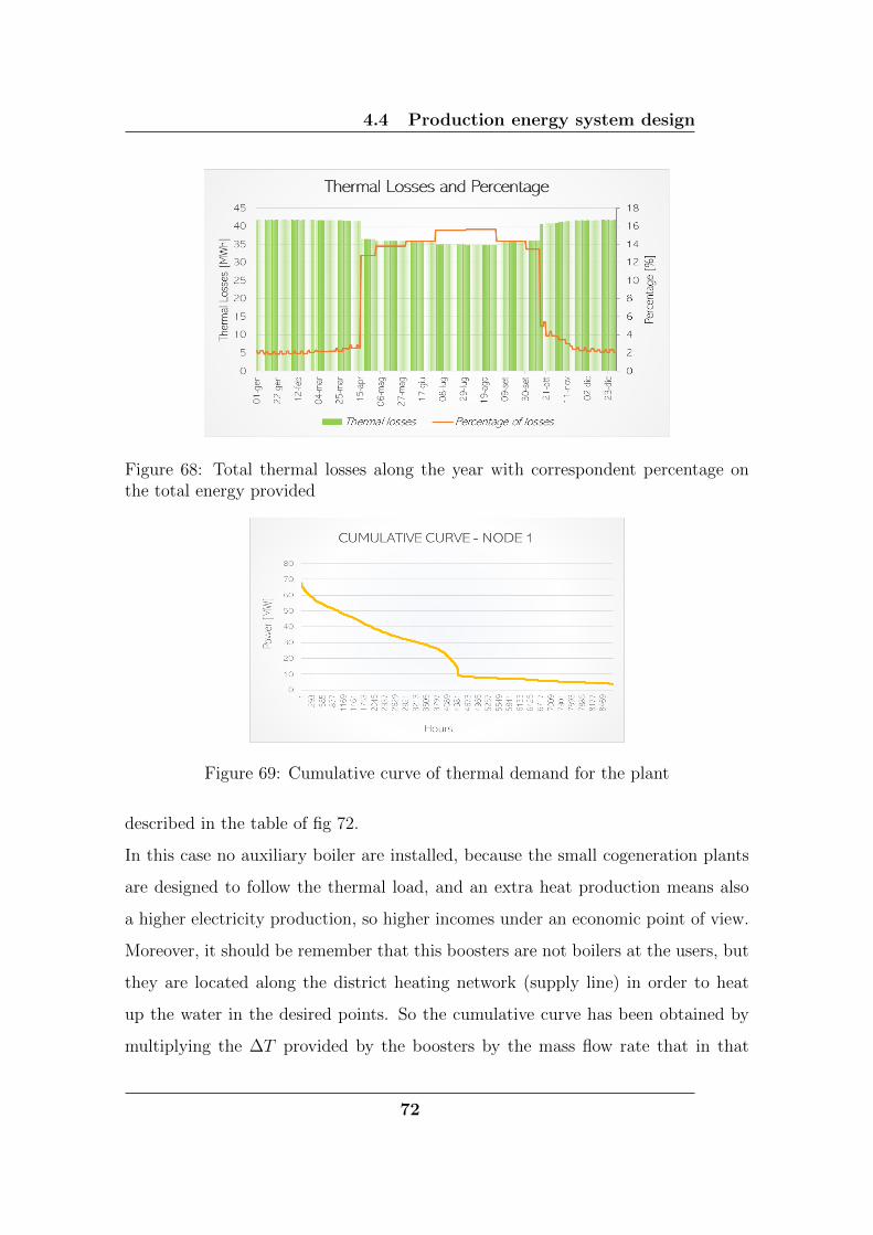
4.4 Production energy system design
Figure 68: Total thermal losses along the year with correspondent percentage onthe total energy provided
Figure 69: Cumulative curve of thermal demand for the plant
described in the table of fig 72.
In this case no auxiliary boiler are installed, because the small cogeneration plants
are designed to follow the thermal load, and an extra heat production means also
a higher electricity production, so higher incomes under an economic point of view.
Moreover, it should be remember that this boosters are not boilers at the users, but
they are located along the district heating network (supply line) in order to heat
up the water in the desired points. So the cumulative curve has been obtained by
multiplying the ∆T provided by the boosters by the mass flow rate that in that
72

4.4 Production energy system design
Figure 70: Cumulative curve of thermal demand for a non industrial user
Figure 71: Cumulative curve of thermal demand for an industrial user
instant of time passes through that particular point.
Figure 72: Configuration of the plant
The thermal power of this boosters goes from 420 kW to 5.3 MW. For this reason
they have been grouped in three different categories:
1. MICRO TURBINE
This is the case of booster 11 and booster 14, that - considering the ratio
73
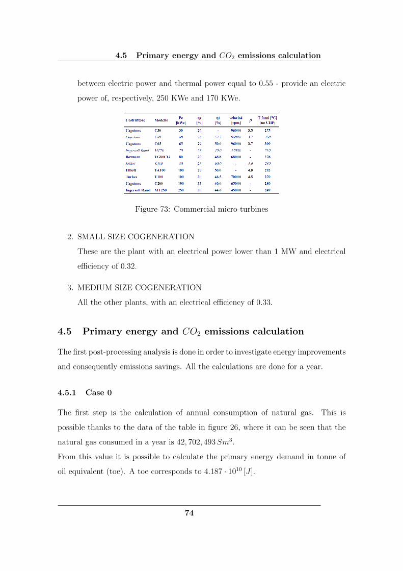
4.5 Primary energy and CO2 emissions calculation
between electric power and thermal power equal to 0.55 - provide an electric
power of, respectively, 250 KWe and 170 KWe.
Figure 73: Commercial micro-turbines
2. SMALL SIZE COGENERATION
These are the plant with an electrical power lower than 1 MW and electrical
efficiency of 0.32.
3. MEDIUM SIZE COGENERATION
All the other plants, with an electrical efficiency of 0.33.
4.5 Primary energy and CO2 emissions calculation
The first post-processing analysis is done in order to investigate energy improvements
and consequently emissions savings. All the calculations are done for a year.
4.5.1 Case 0
The first step is the calculation of annual consumption of natural gas. This is
possible thanks to the data of the table in figure 26, where it can be seen that the
natural gas consumed in a year is 42, 702, 493Sm3.
From this value it is possible to calculate the primary energy demand in tonne of
oil equivalent (toe). A toe corresponds to 4.187 · 1010 [J ].
74

4.5 Primary energy and CO2 emissions calculation
Now it is necessary to calculate tonnes of oil equivalent to 1 Sm3 of natural gas:
1 [Sm3] · LHV[MJ
Sm3
]= 35.046MJ = 3.5046 · 107 [J ] (63)
This means that the conversion coefficient kc from Sm3 of natural gas to toe is:
kc
[Sm3
toe
]=
4.187 · 1010
3.5046 · 107= 1, 195 (64)
Q0NG [toe] =
Q0NG [Sm3]
kc= 35, 736.8 toe (65)
At this point the second parameter of the analysis must be studied. As explained
in the introduction of this work one of the main aim of district heating network is
to reduce Carbon Dioxide emissions in the atmosphere. In order to calculate the
quantity of CO2 that the combustion of natural gas releases in the atmosphere, the
table in figure 9 is taken as reference. It is provided by the Italian Ministry of
Environment (MATTM, Ministero dell’ambiente e della tutela del territorio e del
mare).
Table 9: Emission factor from national inventory of UNFCCC (mean 2016-2018)
Combustibile U.d.m. Fattore emissione (tCO2/U.d.m.)Gas naturale (metano) 1000 Stdm3 1.975
The emission factor that the Italian Ministry of Environment provides is
EF = 1.975
[tCO2
1000Sm3
](66)
This means that the tonnes of CO2 emitted yearly from these users that burns
natural gas for heating and hot water is:
Q0CO2 =
Q0NG [Sm3]
1000· EF = 42, 702.493 · 1.919 = 81, 946.08 tonCO2 (67)
75

4.5 Primary energy and CO2 emissions calculation
4.5.2 Case 1: substitution with centralized generation
In order to calculate the parameters that are object of this study the first thing to
know is the natural gas consumption of this configuration. ENG,plant is the primary
thermal energy provided with the combustion of natural gas in the plant, while
ENG,boiler in the auxiliary boiler.
ENG,plant =Eel,plant
ηel,plant=
132, 723
0.35= 379, 211MWh (68)
ENG,boiler =Eth,plant
ηth,boiler=
138, 748
0.9= 154, 164MWh (69)
ENG,tot = ENG,boiler + ENG,plant = 533, 375MWh (70)
Now with the Low Heating Value (LHV) of natural gas [25] it is possible to
calculate the amount of fuel burned:
ENG,tot [MJ ] = ENG,tot [MWh] · 3600 = 1.920 · 109MJ , (71)
and consequently the primary energy consumption QNG.
Q1NG =
ENG,tot [MJ ]
LHV
[MJ
Sm3
] = 5.4789 · 107 [Sm3] (72)
With the conversion coefficient kc the calculation of primary energy in toe is per-
formed:
Q1NG [toe] =
Q1NG [Sm3]
kc= 45, 848.9 toe , (73)
and eventually the CO2 emissions through the emission factor EF.
Q1CO2 =
Q1NG [Sm3]
1000· EF = 5.904 · 104 · 1.919 = 105, 140.9 tonCO2 (74)
76
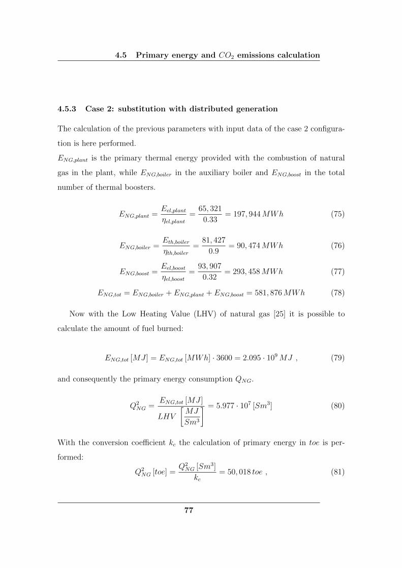
4.5 Primary energy and CO2 emissions calculation
4.5.3 Case 2: substitution with distributed generation
The calculation of the previous parameters with input data of the case 2 configura-
tion is here performed.
ENG,plant is the primary thermal energy provided with the combustion of natural
gas in the plant, while ENG,boiler in the auxiliary boiler and ENG,boost in the total
number of thermal boosters.
ENG,plant =Eel,plant
ηel,plant=
65, 321
0.33= 197, 944MWh (75)
ENG,boiler =Eth,boiler
ηth,boiler=
81, 427
0.9= 90, 474MWh (76)
ENG,boost =Eel,boost
ηel,boost=
93, 907
0.32= 293, 458MWh (77)
ENG,tot = ENG,boiler + ENG,plant + ENG,boost = 581, 876MWh (78)
Now with the Low Heating Value (LHV) of natural gas [25] it is possible to
calculate the amount of fuel burned:
ENG,tot [MJ ] = ENG,tot [MWh] · 3600 = 2.095 · 109MJ , (79)
and consequently the primary energy consumption QNG.
Q2NG =
ENG,tot [MJ ]
LHV
[MJ
Sm3
] = 5.977 · 107 [Sm3] (80)
With the conversion coefficient kc the calculation of primary energy in toe is per-
formed:
Q2NG [toe] =
Q2NG [Sm3]
kc= 50, 018 toe , (81)
77

4.5 Primary energy and CO2 emissions calculation
and eventually the CO2 emissions through the emission factor EF.
Q2CO2 =
Q2NG [Sm3]
1000· EF = 4.647 · 104 · 1.919 = 118, 048.83 tonCO2 (82)
78
5 Economic Analysis
5 Economic Analysis
In order to analyze the economic feasibility [18] of this project in necessary to cal-
culate OPEX and CAPEX of the entire installation:
• CAPEX is the initial investment cost that the plant owner pays at time t=0
(Total Plant Cost TPC).
• OPEX is the set of costs or incomes that every year, until the end of life of
the plant, the plant itself produces.
Once this parameters are calculated, it is possible to implement a cashflow analysis.
In this way all the movement of money can be identified: inflow (sale of goods and
services, loans, lines of credit, asset sales) and outflow (business expenditures, loan
payments, business purchases).
The cashflow analysis is performed from year 0 (the initial investment) until the
end of life of the plant, that in this case is supposed to be 20 years. In the year 0
of construction is considered only the cost of investment. From year 1 on, instead,
depreciation rate, incomes and operating cost (OPEX) have te be considered.
The depreciation rate DR is defined as:
DR =TPC [e]
tdep(83)
where TPC is the total plant cost and tdep is the depreciation time, whose standard
value is 10 years.
The parameters that has to be calculated in order to performed this analysis are:
• Total Plant Cost (TPC), which is practically the investment cost, so the total
outflow of year 0 of construction:
CAPEXtot = Cinv,plant + Cinv,boilers + Cinv,pump + Cinst,network (84)
79

5 Economic Analysis
where Cplant is the total cost of investment needed to build the cogeneration
plant and, in the second case, all the thermal boosters; Cboilers is the cost of
construction of auxiliary boilers, Cpump cost of construction of pumping system
and Cnetwork is the cost of installation of district heating network in the urban
area.
• The overall yearly cost for the following years (from 1 to 20), defined as:
Costs
[e
year
]= COPEX,plant+COPEX,boilers+COPEX,pump+Cmaint,network (85)
where all the OPEX cost are yearly maintenance costs for those systems.
• The Incomes, which are calculated depending on the subsidy for energy ex-
ported to the grid:
Incomes
[e
year
]= Incomesel + Incomesth (86)
where Incomesel come from the electrical energy sold and Incomesth from the
thermal energy sold.
Once all these parameters are known, the cash flow can be eventually calculated:
Cash flow
[e
year
]= Incomes− Costs− t · (Incomes− Costs−DR) (87)
where t is the tax rate (in Italy is considered t = 0.43) which has to be applied only
if Incomes − Costs > 0; while DR (Depreciation Rate) has to be applied only for
the depreciation time, i.e. for the first 10 years.
At this point a method is necessary in order to consider the present value of
money, in this way the present cash flow and the Net Present Value (NPV), Pay
80

5.1 Case 1: Centralized generation
Back Time (PBT) can be analyzed.
Present cash flow
[e
year
]= Cash flow · Discounting factor (88)
where Discounting factor is defined as
Discounting factor = (1 +WACC)−(n−n0) (89)
WACC is Weight Average Cost of Capital, and it takes into account which percent-
age of the initial investment is covered by debt and which by equity. It is expressed
as:
WACC = ke · ce + kd · cd · (1− t) (90)
where kd is the percentage of debt, ke the percentage of equity, cd the cost of debt,
ce the cost of equity.
At this point the Cumulative Cash Flow (CCF) can be determined as
CCFj =
j∑n=0
Present cash flown (91)
The year in which the CCF stars to be positive (NetPresent V alue > 0) is the
year in which all the project starts to earn money, and it is called Payback Time,
PBT.
5.1 Case 1: Centralized generation
5.1.1 CAPEX
1. COGENERATION PLANT
In order to estimate the quantities defined in the previous chapter, the values
in figure 74 [19],[20] have been considered.
In this case the Cinv,plant is simple to calculate, knowing the unit cost cinv,plant
81

5.1 Case 1: Centralized generation
Figure 74: Parameters taken into consideration for economic analysis
in table 74:
Cinv,plant = cinv,plant
[e
MW
]· Pel,plant [MWe] = 900, 000 · 50 = 45, 000, 000e
(92)
2. AUXILIARY BOILER
The italian GSE (Gestore Servizi Energetici) provides the following table (75)
that summarizes the costs for a boiler.
Figure 75: Economic costs provided by GSE [17]
These data are taken from a GSE study [17] that concerns the application
of CHP production with district heating. The value of R are calculated tak-
ing into consideration industrial investment, operating and financial costs. It
strongly depend also on retail to the users price.
Following these data the investment cost for auxiliary boiler is easily calculated
as:
Cinv,boiler = cinv,boiler
[e
MW
]·Pel,boiler [MWe] = 100, 000 · 130 = 13, 000, 000e
(93)
82
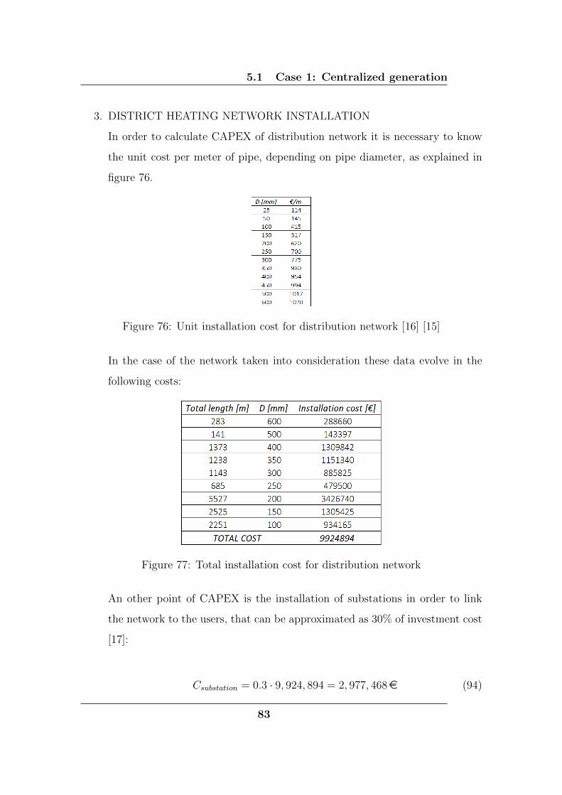
5.1 Case 1: Centralized generation
3. DISTRICT HEATING NETWORK INSTALLATION
In order to calculate CAPEX of distribution network it is necessary to know
the unit cost per meter of pipe, depending on pipe diameter, as explained in
figure 76.
Figure 76: Unit installation cost for distribution network [16] [15]
In the case of the network taken into consideration these data evolve in the
following costs:
Figure 77: Total installation cost for distribution network
An other point of CAPEX is the installation of substations in order to link
the network to the users, that can be approximated as 30% of investment cost
[17]:
Csubstation = 0.3 · 9, 924, 894 = 2, 977, 468e (94)
83

5.1 Case 1: Centralized generation
Once obtained these values Cinst,network can be calculated as:
Cinst,network = Cinst,pipe + Csubstation = 12, 902, 362e (95)
4. PUMPING SYSTEM
The investment cost of the pumping system is considered as 450,000e for a
400 kW system [21].
So the total investment cost at year 0 of construction, according to equation (84),
is:
CAPEXtot = 32, 400, 000 + 13, 000, 000 + 12, 902, 362 + 450, 000 = 58, 752, 362e
(96)
5.1.2 OPEX
1. COGENERATION PLANT
Always following figure 74, the yearly unit cost linked to Operation & Main-
tenance (cO&M,plant) is equal to 40,000$/MW that, considering the current
exchange rate (0.91, [24]), becomes:
cO&M,plant[e] = cO&M,plant[$] · 0.91 = 36, 400e (97)
CO&M,plant = Cinv,plant ·Pel,plant = 36, 400
[e
MW
]· 50 [MW ] = 1, 820, 000
e
year(98)
The other operational cost is the energy source: natural gas. In order to
estimate this cost, with reference to ARERA [22], the price of natural gas is
estimated being 29 e/MWh. These MWh is the quantity of energy produced
burning the natural gas and it is obtained by dividing the quantity of electrical
84

5.1 Case 1: Centralized generation
energy produced in a year by the thermal efficiency:
ENG =Eel
ηel=
132, 724
0.35= 379, 211MWh (99)
The operation in equation 99 is possible because the value of LHV provided
by this authority (the same ARERA) it is the value that has been used in this
work. At this point it is possible to estimate the annual cost of natural gas of
the cogeneration plant:
CNG,plant = ENG · cNG = 10, 617, 912e
year(100)
At the end it can be calculated the total operational plant cost:
COPEX,plant = CO&M,plant + CNG,plant = 12, 437, 912e
year(101)
2. AUXILIARY BOILER
Looking at figure 75, the unit cost of operation & maintenance for boilers is 3
e/MWh, consequently:
CO&M,boiler = cO&M,boiler · Eboiler[MWh] = 3 · 138, 748 = 416, 245e
year(102)
Also in the case of auxiliary boiler the natural gas cost has to be considered:
CNG,boiler = cNG,boiler ·Eboiler
ηboiler= 29 · 138, 748
0.9= 4, 313, 813
e
year(103)
and the total operational cost is:
COPEX,boiler = CO&M,boiler + CNG,boiler = 4, 730, 057e
year(104)
3. DISTRICT HEATING NETWORK
85

5.1 Case 1: Centralized generation
Concerning the OPEX, the network unit maintenance cmaint,network can be
identified in the value of 1.9 e/MWh [17], that multiplied for the total energy
provided to the network (ETOT ) can bring to the total OPEX cost of the
network.
COPEX,net = cO&M,net · Etot = 1.9 · 379, 974.426 = 721, 951e
year(105)
4. PUMPING SYSTEM
The operating cost for pumping system (cOPEX,pump) can be approximated as
1.6 e/MWh [15]. The yearly energy provided by the pumps to the network
Epump has already been calculated and it is equal to 1266 MWh, but that unit
cost refers to the heat provided to the system, thus:
COPEX,pumps = cOPEX,pumps · ETOT = 386, 106e
year(106)
Now that all the costs are calculated it necessary to evaluate the Incomes de-
scribed in previous chapter. As already explained the Incomes are composed of two
different terms, because the owner of the cogeneration plant sells both electricity to
grid and thermal energy to the district heating network users.
The unit revenue for the sale of electrical energy and heat for district heating
can be observed in figure 75: rsale,el = 57e/MWh (78 in summer) and rsale,th =
94.8e/MWh. In this way the incomes can be calculated:
Incomesel = rsale,el · Eel = 8, 262, 062e
year(107)
Incomesth = rsale,th · (ETOT − Eloss) = 34, 477, 986e
year(108)
86

5.1 Case 1: Centralized generation
5.1.3 Cashflow Analysis
First point of the analysis is the depreciation rate DR, calculated as:
DR =CAPEXtot
tdep=
71, 352, 362
10= 7, 135, 236.2e (109)
Consequently, the DR has to be applied only for the first 10 years. This brings to
two different definitions of CashF low:
CashF low1
[e
year
]= Incomes− Costs− t · (Incomes− Costs−DR) (110)
for the first 10 years and
CashF low2
[e
year
]= Incomes− Costs− t · (Incomes− Costs) (111)
for the remaining years.
Weighted Average Cost of Capital for calculation of discounting factor is estimated
to be 5% [17]. With these data it is possible to calculate all the parameters required,
as the figure 78 shows.
For the calculation of the Payback Time a linear approximation of NPV curve
is applied from year 4 to 5. In this way a line is constructed and imposing the CCF
equal to 0 it is possible to find the point in which the NPV curve meets the x-axis:
PBT = 4 +11, 026, 368
2, 303, 484 + 11, 026, 368= 4.83 years (112)
This means that after less than 5 years all the money spent in the initial investment
is recovered.
The Net Present value at 20 years that is equal to NPV=126,118,292e.
87

5.1 Case 1: Centralized generation
Figure 78: Cash flow analysis (case 1)
Figure 79: Cumulative Cash Flow for every year of system lifetime (case 1)
88

5.2 Case 2: Distributed Generation
5.2 Case 2: Distributed Generation
1. COGENERATION PLANT
The procedure is similar to the plant of case 1, with different values, like figure
80 shows [19],[20].
Figure 80: Parameters taken into consideration for economic analysis
In this case the Cinv,plant is:
Cinv,plant = cinv,plant
[e
MW
]·Pel,plant [MWe] = 1, 000, 000 · 25 = 25, 000, 000e
(113)
Always following figure 74, the yearly unit cost linked to Operation & Main-
tenance (cO&M,plant) is equal to 45,500e/MW:
CO&M,plant = cO&M,plant ·Pel,plant = 45, 500
[e
MW
]·25 [MW ] = 1, 137, 500
e
year(114)
Always with reference to ARERA [22], the price of natural gas is estimated
being 29 e/MWh.
ENG =Eel
ηel=
65, 321
0.33= 197, 943.8MWh (115)
At this point it is possible to estimate the annual cost of natural gas of the
cogeneration plant:
CNG,plant = ENG · cNG = 5, 740, 330e
year(116)
89

5.2 Case 2: Distributed Generation
At the end it can be calculated the total operational plant cost:
COPEX,plant = CO&M,plant + CNG,plant = 6, 877, 830e
year(117)
2. AUXILIARY BOILER
Figure (75) is valid also for this case, so the calculation can proceed:
Cinv,boiler = cinv,boiler
[e
MW
]· Pel,boiler [MWe] = 100, 000 · 68 = 6, 800, 000e
(118)
Looking at figure 75, the unit cost of operation & maintenance for boilers is 3
e/MWh, consequently:
CO&M,boiler = cO&M,boiler · Eboiler[MWh] = 3 · 81, 427 = 244, 281e
year(119)
Also in the case of auxiliary boiler the natural gas cost has to be considered:
CNG,boiler = cNG,boiler ·Eboiler
ηboiler= 29 · 81, 427
0.9= 2, 623, 759
e
year(120)
and the total operational cost is:
COPEX,boiler = CO&M,boiler + CNG,boiler = 2, 868, 040e
year(121)
3. THERMAL BOOSTERS
For the evaluations of the costs of micro-turbine, mini and medium size cogen-
eration cost curves have been applied in order to consider the different size of
each booster. The data for the construction of these curves ([23]) have been
gathered and sorted plots in figure 81 and 82:
It is possible to notice that these costs are higher than the unit cost of case 1,
this because in the case of smaller sizes the amount of money that is necessary
90

5.2 Case 2: Distributed Generation
Figure 81: Unit investment cost for the construction of gas turbines [23]
Figure 82: Unit Operation & Maintenance cost for gas turbines [23]
to spend for a single unit of energy increases.
Due to the different configuration (at lower temperature) the energy that the
system has to provide to district heating network is slightly reduced, thanks
to the lower thermal losses. Nevertheless this little drop of thermal demand
is not sufficient to justify the higher investment that distributed generation
requires, as will be clarified below.
Knowing these data the calculation of the total costs of the thermal boosters
91

5.2 Case 2: Distributed Generation
is performed.
Cinv,boost = cinv,boost
[e
MW
]·∑j
P el,boostj [MWe] = 31, 176, 092e (122)
CO&M,boost = cO&M,boost ·∑j
Eboost[MWh] = 1, 878, 986e
year(123)
Also in the case of thermal boosters the natural gas cost has to be considered:
CNG,boost = cNG ·Eel,boost
ηel,boost= 29 · 93, 906.6
0.32= 8, 510, 286
e
year(124)
and the total operational cost is:
COPEX,boost = CO&M,boost + CNG,boost = 10, 389, 272e
year(125)
4. OTHER POINTS
District heating network and pumping system are supposed not to vary with
respect to case 1.
The unit revenue for the sale of electrical energy and heat for district heating
are the same of previous case: rsale,el = 57e/MWh (78 in summer) and rsale,th =
94.8e/MWh. In this way the incomes can be calculated:
Incomesel = rsale,el · Eel = 9, 911, 947e
year(126)
Incomesth = rsale,th · (ETOT − Eloss) = 33, 829, 907e
year(127)
Supposing other parameters for cash flow analysis unchanged it is possible to
perform the calculation done for case 1 with the new input data, obtaining the
following.
The calculation of the Payback Time is performed with the same method of the
92

5.2 Case 2: Distributed Generation
Figure 83: Cash flow analysis for case of distributed generation
previous case:
PBT = 5 +5, 269, 599
6, 977, 889 + 5, 269, 599= 5.43 years (128)
Figure 84: Cumulative Cash Flow in time for distributed generation case
The Net Present value at 20 years that is equal to NPV=112,652,545e.
93
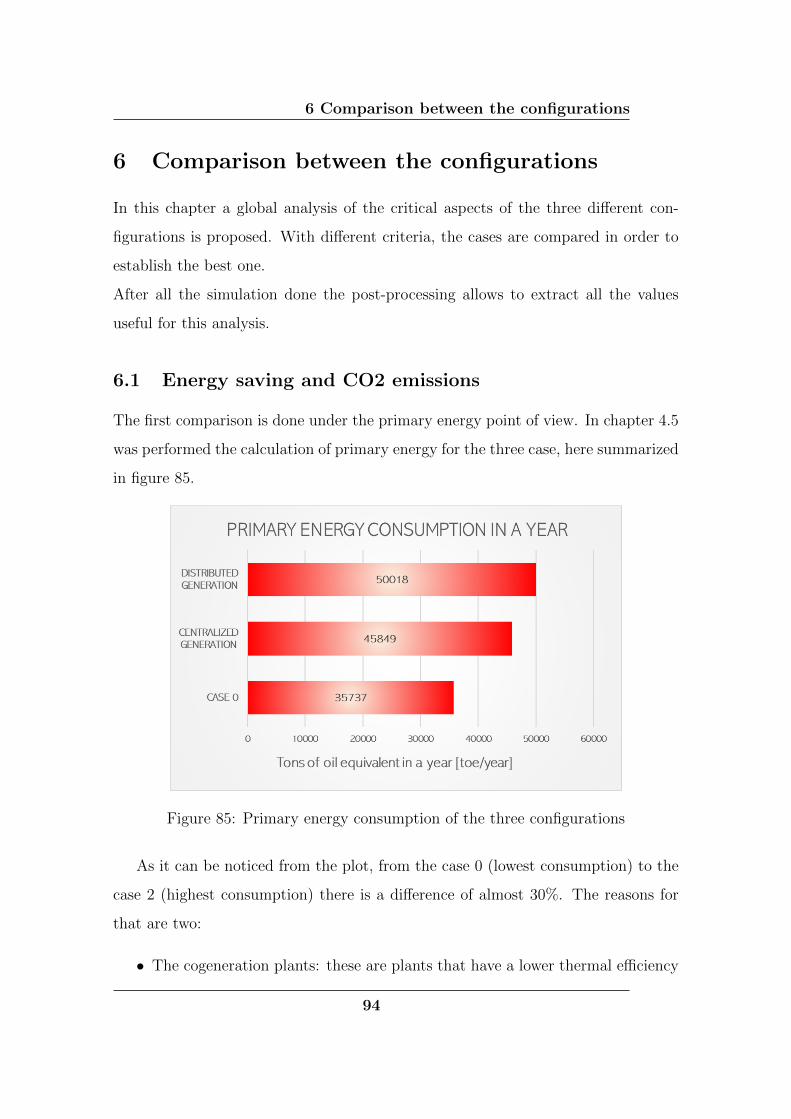
6 Comparison between the configurations
6 Comparison between the configurations
In this chapter a global analysis of the critical aspects of the three different con-
figurations is proposed. With different criteria, the cases are compared in order to
establish the best one.
After all the simulation done the post-processing allows to extract all the values
useful for this analysis.
6.1 Energy saving and CO2 emissions
The first comparison is done under the primary energy point of view. In chapter 4.5
was performed the calculation of primary energy for the three case, here summarized
in figure 85.
Figure 85: Primary energy consumption of the three configurations
As it can be noticed from the plot, from the case 0 (lowest consumption) to the
case 2 (highest consumption) there is a difference of almost 30%. The reasons for
that are two:
• The cogeneration plants: these are plants that have a lower thermal efficiency
94

6.1 Energy saving and CO2 emissions
with respect to the local small size boilers. On the other hand they have also
an electrical efficiency because they produce both electricity and heat: this is
an aspect that has to be taken into consideration for a complete and coherent
analysis.
• The smaller size of plants in case 2: in the distributed heat generation case
the size of the thermal boosters is obviously smaller than the case of a big
plant. This implies a smaller efficiency of the single booster with respect to
the higher size plant.
Always in chapter 4.5 the procedure for the calculation of CO2 emissions is
described, and the values obtained are listed. Here are represented in the plot of
figure 86.
Figure 86: CO2 emissions for the three configurations
The orange bars represent the CO2 emitted in a year in total while the green bar
represents the Carbon Dioxide that would have been emitted in order to produce
the electrical energy produced in the plants. In order to perform this calculation the
medium global efficiency for the production of electrical energy is considered equal
95
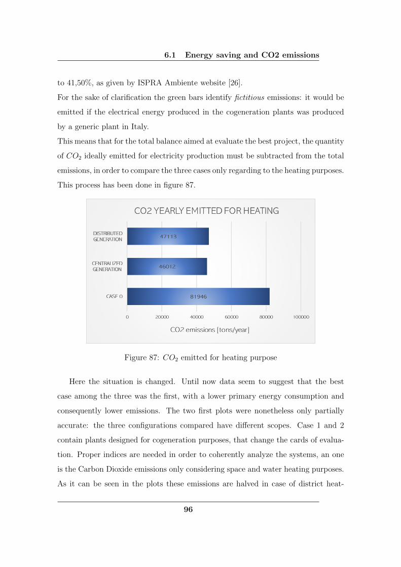
6.1 Energy saving and CO2 emissions
to 41,50%, as given by ISPRA Ambiente website [26].
For the sake of clarification the green bars identify fictitious emissions: it would be
emitted if the electrical energy produced in the cogeneration plants was produced
by a generic plant in Italy.
This means that for the total balance aimed at evaluate the best project, the quantity
of CO2 ideally emitted for electricity production must be subtracted from the total
emissions, in order to compare the three cases only regarding to the heating purposes.
This process has been done in figure 87.
Figure 87: CO2 emitted for heating purpose
Here the situation is changed. Until now data seem to suggest that the best
case among the three was the first, with a lower primary energy consumption and
consequently lower emissions. The two first plots were nonetheless only partially
accurate: the three configurations compared have different scopes. Case 1 and 2
contain plants designed for cogeneration purposes, that change the cards of evalua-
tion. Proper indices are needed in order to coherently analyze the systems, an one
is the Carbon Dioxide emissions only considering space and water heating purposes.
As it can be seen in the plots these emissions are halved in case of district heat-
96

6.1 Energy saving and CO2 emissions
ing network with respect to the case without it, and in particular the centralized
generation is even better than the distributed generation. The main reason is that,
despite a higher production of electricity in case 2, the efficiencies of small plants
are lower than the efficiency of a single big plant. An other index useful in order to
properly compare the cases is the useful energy for unit of primary energy (figure
88).
Figure 88: Index of efficiency: how much useful energy is provided to the system[MWh] with one toe of primary energy
It is a sort of efficiency (ε), with the primary energy calculated in toe with the
objective of highlight the primary energy utilization.
ε =Euseful [MWh]
Eprimary [toe](129)
For the evaluation of Euseful the control volume ends at the inlet and outlet of
secondary supply and return: it is practically the energy provided to the water at
the level of substations for district heating and boilers for case 0, and it corresponds
to the energy sold.
It is clear how in this case the district heating is better than burning directly natural
97
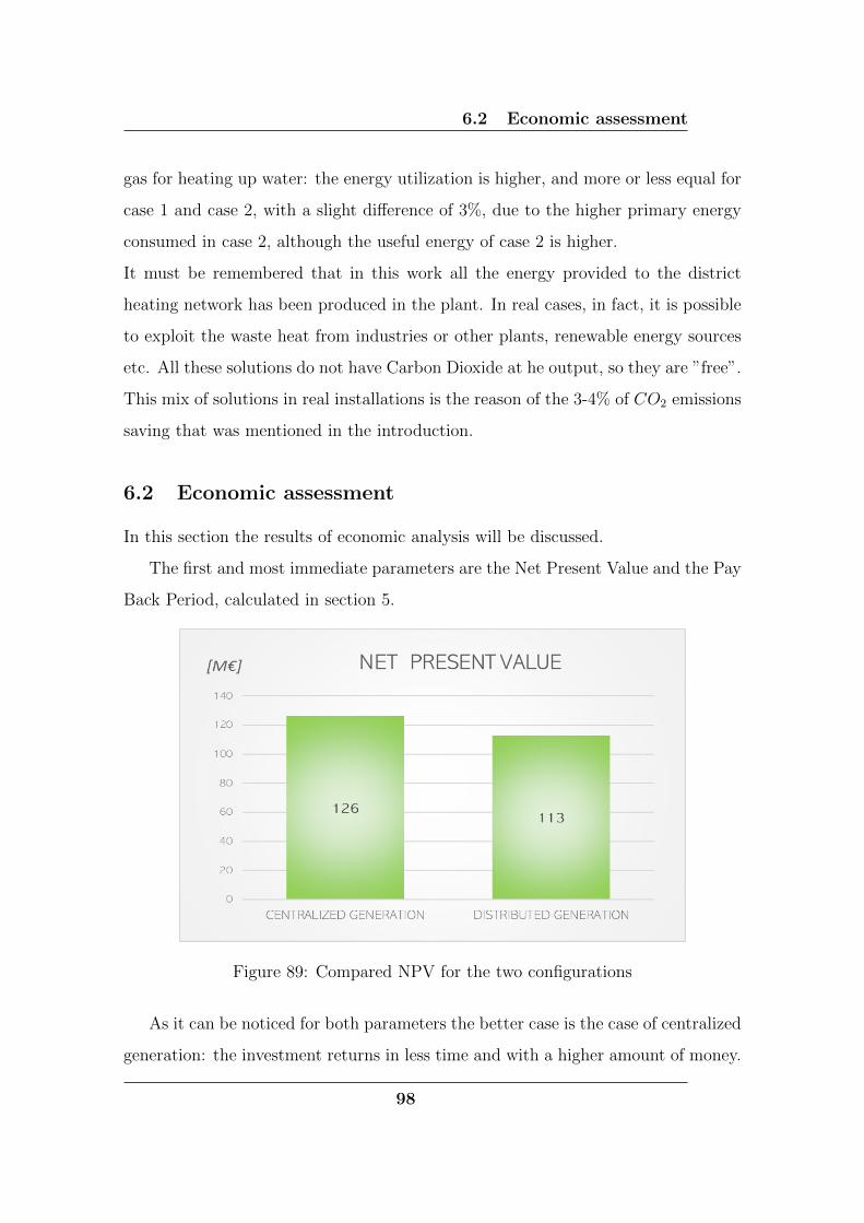
6.2 Economic assessment
gas for heating up water: the energy utilization is higher, and more or less equal for
case 1 and case 2, with a slight difference of 3%, due to the higher primary energy
consumed in case 2, although the useful energy of case 2 is higher.
It must be remembered that in this work all the energy provided to the district
heating network has been produced in the plant. In real cases, in fact, it is possible
to exploit the waste heat from industries or other plants, renewable energy sources
etc. All these solutions do not have Carbon Dioxide at he output, so they are ”free”.
This mix of solutions in real installations is the reason of the 3-4% of CO2 emissions
saving that was mentioned in the introduction.
6.2 Economic assessment
In this section the results of economic analysis will be discussed.
The first and most immediate parameters are the Net Present Value and the Pay
Back Period, calculated in section 5.
Figure 89: Compared NPV for the two configurations
As it can be noticed for both parameters the better case is the case of centralized
generation: the investment returns in less time and with a higher amount of money.
98
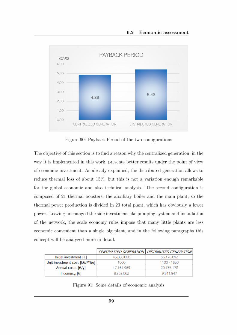
6.2 Economic assessment
Figure 90: Payback Period of the two configurations
The objective of this section is to find a reason why the centralized generation, in the
way it is implemented in this work, presents better results under the point of view
of economic investment. As already explained, the distributed generation allows to
reduce thermal loss of about 15%, but this is not a variation enough remarkable
for the global economic and also technical analysis. The second configuration is
composed of 21 thermal boosters, the auxiliary boiler and the main plant, so the
thermal power production is divided in 23 total plant, which has obviously a lower
power. Leaving unchanged the side investment like pumping system and installation
of the network, the scale economy rules impose that many little plants are less
economic convenient than a single big plant, and in the following paragraphs this
concept will be analyzed more in detail.
Figure 91: Some details of economic analysis
99

6.2 Economic assessment
The values in figure 91 are concerning only the energy production: pumping
system and distribution network are excluded. The reason is the willing to focus
only on the parameters that cause the differences, and the items excluded are equal
in the two cases, so they do not affect the analysis that is going to be performed.
From the figure 91 are taken the reasons of the convenience of invest in the
centralized energy production configuration, that are analyzed in detail here:
• INITIAL INVESTMENT
The first difference between the two cases is already in initial investment. As
already said, this is due to the economy of scale rules. The unit investment
cost, in fact, is lower in the case of centralized generation. The presence of a
big plant reduces the cost per unit of energy, even of 50% for the smaller size
plants.
• ANNUAL COSTS
The situation is the same for O&M annual costs, around 7 e/MWh per year for
distributed generation and 36,400 e/MWe per year. This causes a difference
in the annual costs of about 3 million euro, tha multiplied by 20 year of lifetime
is anything but negligible.
• INCOMES
While the incomes from the sale of heating is equal in the two cases because
connected to the users thermal demand, in case 2 the incomes from the sale of
electricity is 1.5 million of euro higher. This is due to the higher percentage of
heat provided with cogeneration: in the table of figures 64 and 72 is evident
how the percentage of heat provided with the boiler (so without cogeneration)
is about 22% in case 2 and about 36% in case 1. This last higher percentage
means that a higher amount of heat is provided without correlated production
of electrical energy, from this the lower incomes. But the higher incomes do
not compensate the higher initial investment.
100
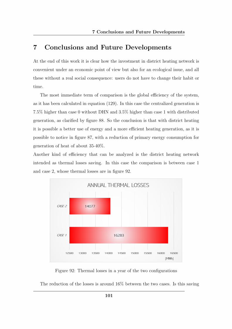
7 Conclusions and Future Developments
7 Conclusions and Future Developments
At the end of this work it is clear how the investment in district heating network is
convenient under an economic point of view but also for an ecological issue, and all
these without a real social consequence: users do not have to change their habit or
time.
The most immediate term of comparison is the global efficiency of the system,
as it has been calculated in equation (129). In this case the centralized generation is
7.5% higher than case 0 without DHN and 3.5% higher than case 1 with distributed
generation, as clarified by figure 88. So the conclusion is that with district heating
it is possible a better use of energy and a more efficient heating generation, as it is
possible to notice in figure 87, with a reduction of primary energy consumption for
generation of heat of about 35-40%.
Another kind of efficiency that can be analyzed is the district heating network
intended as thermal losses saving. In this case the comparison is between case 1
and case 2, whose thermal losses are in figure 92.
Figure 92: Thermal losses in a year of the two configurations
The reduction of the losses is around 16% between the two cases. Is this saving
101
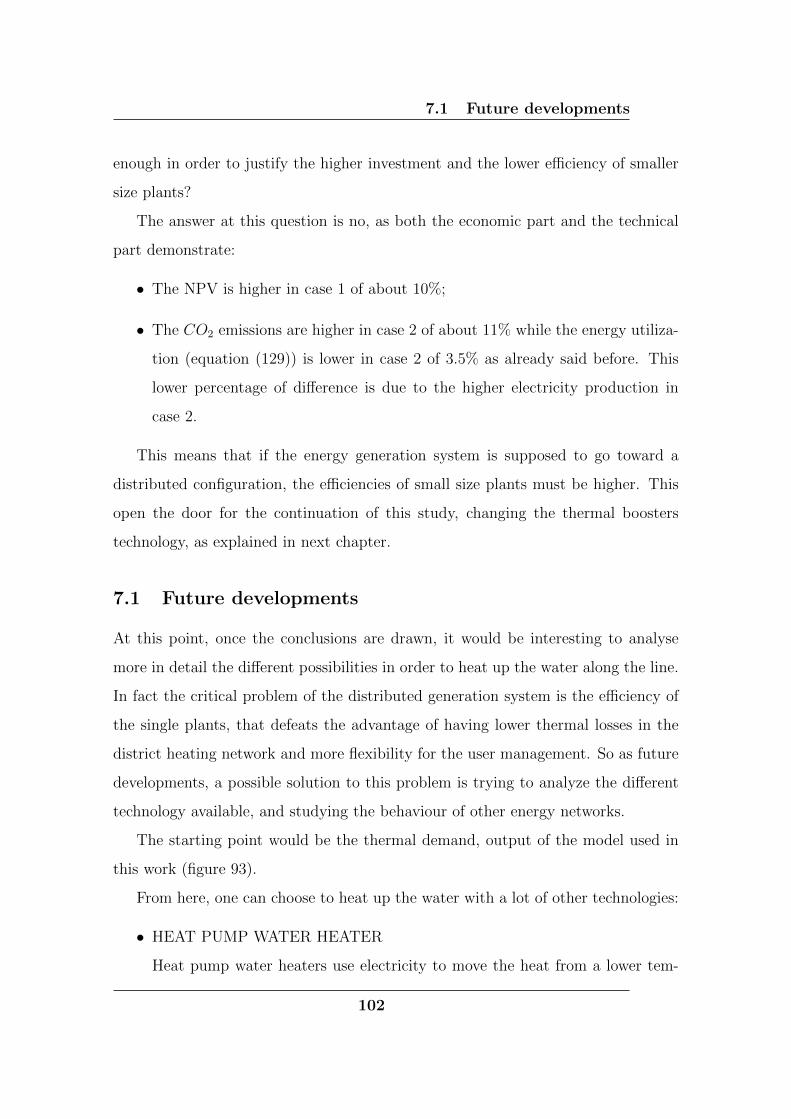
7.1 Future developments
enough in order to justify the higher investment and the lower efficiency of smaller
size plants?
The answer at this question is no, as both the economic part and the technical
part demonstrate:
• The NPV is higher in case 1 of about 10%;
• The CO2 emissions are higher in case 2 of about 11% while the energy utiliza-
tion (equation (129)) is lower in case 2 of 3.5% as already said before. This
lower percentage of difference is due to the higher electricity production in
case 2.
This means that if the energy generation system is supposed to go toward a
distributed configuration, the efficiencies of small size plants must be higher. This
open the door for the continuation of this study, changing the thermal boosters
technology, as explained in next chapter.
7.1 Future developments
At this point, once the conclusions are drawn, it would be interesting to analyse
more in detail the different possibilities in order to heat up the water along the line.
In fact the critical problem of the distributed generation system is the efficiency of
the single plants, that defeats the advantage of having lower thermal losses in the
district heating network and more flexibility for the user management. So as future
developments, a possible solution to this problem is trying to analyze the different
technology available, and studying the behaviour of other energy networks.
The starting point would be the thermal demand, output of the model used in
this work (figure 93).
From here, one can choose to heat up the water with a lot of other technologies:
• HEAT PUMP WATER HEATER
Heat pump water heaters use electricity to move the heat from a lower tem-
102
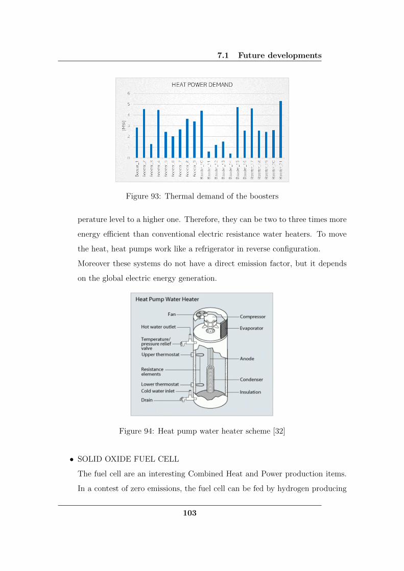
7.1 Future developments
Figure 93: Thermal demand of the boosters
perature level to a higher one. Therefore, they can be two to three times more
energy efficient than conventional electric resistance water heaters. To move
the heat, heat pumps work like a refrigerator in reverse configuration.
Moreover these systems do not have a direct emission factor, but it depends
on the global electric energy generation.
Figure 94: Heat pump water heater scheme [32]
• SOLID OXIDE FUEL CELL
The fuel cell are an interesting Combined Heat and Power production items.
In a contest of zero emissions, the fuel cell can be fed by hydrogen producing
103

7.1 Future developments
heat and power, with zero CO2 emissions.
Alternatively, for a connection with gas network, it can be fed by methane and
hydrogen but in this case there is a Carbon Dioxide emission.
Figure 95: Solid Oxide Fuel Cell basic operation scheme
As already said, an integrate analysis of energy network would be very interest-
ing. In order to do that it is sufficient to extract the values of gas and electricity
consumption for each user node, and using them as input for the network simulation.
The point is that every technology would have its own primary energy consumption
and its own output, in addition a comparative economic analysis would highlight
the different state of art of each different technology in the actual period.
Figure 96: Electricity output of each booster
104

7.1 Future developments
Figure 97: Natural gas consumption of each booster
For the CHP plants described in this work, the analysis would start from this
inputs.
105

REFERENCES
References
[1] https://www.gruppohera.it/gruppo/com media/dossie tlr/articoli/pagina70.html
[2] DHC + Technology Platform, District heating and cooling. A vision toward 2020-2030-2050, March 2012.
[3] Future district heating systems and technologies: On the role of smart energysystems and 4th generation district heating, Lund et al.
[4] Dynamic modelling of local district heating grids with prosumers: A case studyfor Norway, Kauko et al.
[5] Energy storage and smart energy systems, Lund H, Østergaard PA, Connolly D,Ridjan I, Mathiesen BV, Hvelplund F, et al.
[6] Computational comparison of a novel decentralized photovoltaic district heatingsystem against three optimized solar district systems, Hassam ur Rehman, JanneHirvonen, Risto Kosonen, Kai Siren
[7] CHP and heat pumps to balance renewable power production: Lessons from thedistrict heating network in Stockholm, Fabian Levihn
[8] District heating based on biogas from wastewater treatment plant, Alberto Pi-cardo, Victor M. Soltero, M. Estela Peralta, Ricardo Chacartegui
[9] Numerical Design of Thermal Systems, A.Sciacovelli, V. Verda, R.Borchiellini
[10] Del Hoyo Arce I., Herrero Lopez S., Lopez Perez S., Rama M., Klobut K.,Febres J. A., Models for fast modelling of district heating and cooling networks,Renewable and Sustainable Energy Reviews 82 (2018) 1863-1873.
[11] Le equazioni della meccanica dei fluidi, Stefano Lanzoni
[12] Thermo-fluid dynamic model of large district heating networks for analysis ofprimary energy savings, Guelpa E., Sciacovelli A., Verda V., Energy (2017)
[13] Numerical model for the analysis of thermal transients in district heating net-works, Capone, Guelpa, Verda
[14] Dynamic modeling and control of a plate heat exchanger, Hector Bastida, CarlosErnesto Ugalde-Loo, Muditha Abeysekera, Meysam Qadrdan
[15] Studio di una Rete di Teleriscaldamento nel Comune di Padova, Lorenzo Casna
[16] https://www.airu.it/teleriscaldamento/
106

REFERENCES
[17] Valutazione del potenziale nazionale di applicazione della cogenerazione ad altorendimento e del teleriscaldamento efficiente, GSE
[18] Cost Estimation Methodology for NETL Assessments of Power Plant Perfo-mance, NETL
[19] Energia elettrica, anatomia dei costi, RSE Riflessioni sull’Energia
[20] Combined Heat and Power, IEA-ETSAP
[21] https://www.pumpsandsystems.com/estimate-pump-installation-costs
[22] https://www.arera.it/it/dati/gpcfr2.htm
[23] Dispensa del corso di “SISTEMI ENERGETICI”. Argomento: Sistemi Ener-getici (parte 3.2), Prof. Pier Ruggero Spina, Dipartimento di Ingegneria Universitadi Ferrara
[24] https://mercati.ilsole24ore.com/tassi-e-valute/valute/contro-euro/cambio/EURUS.FX
[25] MATTM, https://www.minambiente.it/
[26] http://www.isprambiente.gov.it/
[27] TESTO INTEGRATO DELLE DISPOSIZIONI PER LA REGOLAZIONEDELLE PARTITE FISICHE ED ECONOMICHE DEL SERVIZIO DI BILAN-CIAMENTO DEL GAS NATURALE (TISG), ARERA (Autorita di Regolazioneper Energia Reti e Ambiente)
[28] Piano per il riscaldamento ambientale e il condizionamento della RegionePiemonte [Aggiornamento del Piano regionale per il risanamento e la tutela dellaqualita dell’aria: Stralcio per il riscaldamento ambientale e il condizionamento edisposizioni attuative della legge regionale 28 Maggio 2017 n. 13 (Disposizioni inmateria di rendimento energetico nell’edilizia) - Articolo 21, lettere a), b) e q)]
[29] Sistemi di teleriscaldamento, Vittorio Verda, Dipartimento Energia - Politec-nico di Torino, lecture slides of the course ”Complementi di Energetica”
[30] Studio e caratterizzazione di un modello compatto per l’analisi di sottostazionidi scambio termico di teleriscaldamento, Daniele Farina. Relatore: Prof. VittorioVerda, Correlatore: Ing. Elisa Guelpa
[31] Universita degli Studi di Napoli Federico II, D.E.TE.C. - Dipartimento di En-ergetica, Cogenerazione e trigenerazione: dai principi generali alle applicazioni,Gestione delle Risorse Energetiche, A.A. 2012/2013
[32] https://www.energy.gov/energysaver/water-heating/heat-pump-water-heaters
107