terrain analysis - dst igetdst-iget.in/tutorials/iget_rs_010/iget_rs_010_terrain analysis.pdf ·...

Terrain Analysis

Using QGIS and SAGA

Tutorial ID: IGET_RS_010

This tutorial has been developed by BVIEER as part of the IGET web portal intended to provide easy access to geospatial education. This

tutorial is released under the Creative Commons license. Your support will help our team to improve the content and to continue to offer high

quality geospatial educational resources. For suggestions and feedback please visit www.iget.in.

IGET_RS_010 Terrain Analysis using QGIS and SAGA

2

Terrain Analysis using QGIS and SAGA

Objective: To analyze the topography of a region with respect to its slope, aspect and curvature etc., using a

Digital Elevation Model.

Software: SAGA GIS and Quantum GIS

Level: Intermediate

Time required: 3 Hours

Prerequisites and Geospatial Skills:

1. SAGA and QGIS should be installed on the computer.

2. Familiarity with basic operations in SAGA and QGIS is preferable.

3. An internet connection to fetch ‘Profile Tool’ plugin.

Readings

1. Clarke, K. C. (1995). Chapter 13: Terrain Analysis. In Analytical and Computer Cartography (2nd ed., pp.

249–279). Prentice Hall. Retrieved from http://www.geog.ucsb.edu/~kclarke/AACC/ Chapter13.pdf

2. Aileen, B. (n.d.). Understanding curvature rasters. ArcGIS Resources. Retrieved from

http://blogs.esri.com/esri/arcgis/2010/10/27/understanding-curvature-rasters/

3. Scottish Road Network Landslides Study: Implementation | Transport Scotland. (n.d.). Retrieved June

24, 2013, from http://www.transportscotland.gov.uk/strategy-and-research/publications-and-

consultations/j10107-07.htm

Tutorial Data: SRTM DEM downloaded from http://srtm.csi.cgiar.org has been supplied for this tutorial and

can be downloaded here.

Link

http://www.geog.ucsb.edu/~kclarke/AACC/%20Chapter13.pdf

http://www.geog.ucsb.edu/~kclarke/AACC/%20Chapter13.pdf

http://blogs.esri.com/esri/arcgis/2010/10/27/understanding-curvature-rasters/

http://www.transportscotland.gov.uk/strategy-and-research/publications-and-consultations/j10107-07.htm

http://www.transportscotland.gov.uk/strategy-and-research/publications-and-consultations/j10107-07.htm

http://srtm.csi.cgiar.org/


3

Introduction

While using raster data in the previous tutorials the images were limited to those describing the spectral

properties of the land, however we also have raster datasets that describes the elevation of the land. The elevation

values are stored in the form of a raster grid known as a Digital Elevation Model (DEM). The DEM pixel values

indicate the height of the pixel above the defined vertical datum. Although the DEM itself describes just the

elevation of the land surface, it can be used to derive many interesting and useful data products. These derivatives

are used in almost every field and mostly in hydrological, visibility, ecology and morphological analyses.

DEMs are generated as a product of the satellites like ASTER, CartoSat P5, and the Shuttle Radar

Topography Mission (SRTM). Often user may come across some areas with missing pixel values, these are referred

to as ‘holes’ or ‘sinks’ in the data and are caused by anomalies during the data collection. To alleviate this problem

there exist many algorithms which fill in these sinks by interpolating the elevation of neighboring pixels.

In this tutorial we will learn how to fill the sinks, prepare various products, and visualize DEM data by

using both Quantum GIS and SAGA GIS.

1. Start Quantum GIS → Open the DEM in QGIS by clicking on the ‘Add Raster’ button in the

toolbar or via ‘Layer → Add Raster Layer’. Navigate to the tutorial data folder, click on the DEM file

‘n18_e073_3arc_v1.tif’ and click on ‘Okay’.

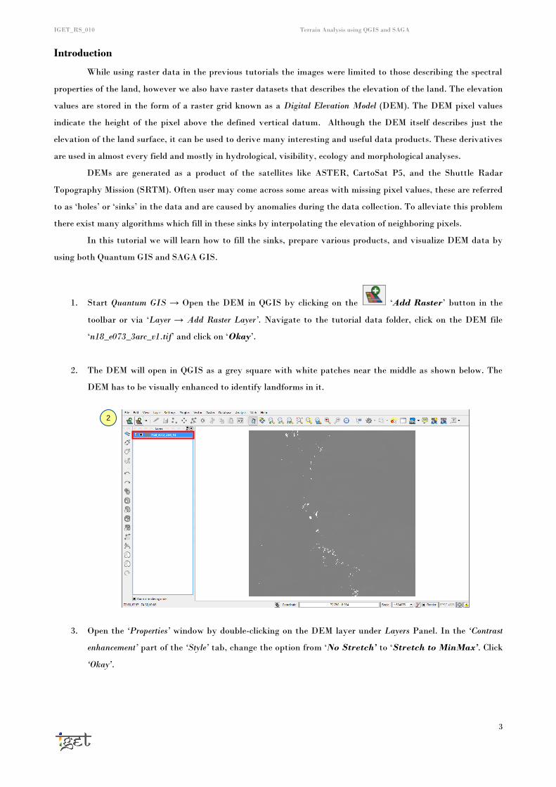
2. The DEM will open in QGIS as a grey square with white patches near the middle as shown below. The

DEM has to be visually enhanced to identify landforms in it.

3. Open the ‘Properties’ window by double-clicking on the DEM layer under Layers Panel. In the ‘Contrast

enhancement’ part of the ‘Style’ tab, change the option from ‘No Stretch’ to ‘Stretch to MinMax’. Click

‘Okay’.

2


4

4. The white patches are the parts of the DEM without any data and generally referred as the holes or sinks

which cause problems in analysis if they are not filled.

5. These sinks are filled by interpolating the pixel values from the neighborhood pixels. To do this use the

‘Fill nodata’ tool (Raster → Analysis → Fill nodata).

6. Fill in the ‘Output file’ as ‘n18_e073_3arc_v1_SinkFilled.tif’ field and ‘check’ the ‘Load into canvas when

finished’. Click ‘Okay’. After successful execution click on ‘OK’ in ‘Finished’ window and ‘close’ the ‘Fill

nodata’ window.

3

5

4


5

7. The corrected DEM will now be loaded into the layers list. If the layer is greyed out, enhance it by doing a

contrast stretch as described in Step 3.

8. Turn off the layer by unchecking the layer in the list . Zoom into

the sink holes and turn it on again to see the interpolated region.

6

7


6

9. Let us view this more explicitly by creating a profile of this area. For this we will use the ‘Profile tool’

plugin.

10. Click on ‘Fetch Python plugins…’ from the Plugins menu and type ‘profile’ in the Filter space. It

shortlist the available plugins from the list. Select the ‘Profile Tool’ and click on ‘Install plugin’. Make

sure the computer is connected to the internet before doing this and click on ‘OK’ to finish and now

‘Close’ the Plugin installer.

11. Open this tool via Plugins → Profile Tool → Terrain Profile. The mouse cursor will change to a ‘+’ sign.

Place the starting point of the profile line by clicking on one side of the sink area. A line will appear which

can be extended across the terrain. Clicking again will set a vertex for the line. This allows us to create a

profile along an irregular path. Double-click on the other side of the area to end the profile line.

8

10


7

12. This will show us a profile of the sink filled DEM. To compare it with the unfill sinks DEM, we will add

the unprocessed DEM to this tool by clicking on the ‘Add Layer’ button. Select

the unprocessed DEM and click on ‘Okay’. Change the colour of the newly added DEM by clicking on the

‘ colour box’ next to the layer name.

13. The second profile may not appear in the graph. If this happens, just draw the profile line again. In the

following figure Red and Green are processed and unprocessed DEM profiles successively.

Task 1: Explain the Profile trends in above figure.

14. This way we can see how the pixel values have been interpolated. Click on the ‘Save as’ button to save

the profile as an image or PDF.

15. Click on ‘Zoom Full’ to see the entire DEM. Now draw a profile line from West to East through the

11

13


8

centre of the DEM.

Task 2: Explain the topography of the area from the above profile and which landforms are represented in

the encircled part of the profile?

16. Close the Quantum GIS. Now we will switch to SAGA to perform a few basic analytical processes on

DEM.

17. Launch SAGA and open the filled DEM image in SAGA by clicking the ‘Load’ button. Navigate to

the DEM file, select it and click ‘Open’ (File types should be set to ‘All files’ to view the DEM).

18. The DEM will be imported into the Data tab list. Double click on it to open in a Map window as shown

above. Click the tab under Object Properties section. This will display the metadata of the

DEM, some part of which is displayed below.

15

18


9

19. As you see, the DEM is in a Geographic Coordinate System (GCS), which means its distance is measured in

degrees (cell size is 0.0008333 degrees). Before carrying out any spatial analysis operations on the DEM, it

will strongly suggest to convert it from a Geographic Coordinate System to a Projected Coordinate System.

20. Open the ‘Coordinate Transformation’ module via Module → Projection → Coordinate Transformation

(Grid). In the module window, under ‘Proj4 Parameters’, change the ‘Projected Coordinate System’ entry to

‘WGS 84 / UTM 43N’. Enter the ‘Grid System’ entries as shown below, and for the ‘Interpolation’ method

we will use ‘Nearest Neighbor’.

21. On clicking ‘Okay’ a window describing the dimensions of the DEM will pop up. Click ‘Okay’ on that as

well.

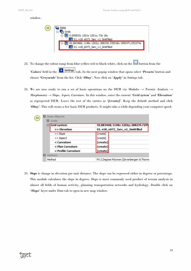
22. The reprojected DEM will now be placed in the Data list. It will now have a different set of descriptors.

You can see the pixel size has been converted from 0.00083333 degrees to 92.88 meters .Open it in a new

18

20


10

window.

23. To change the colour ramp from blue-yellow-red to black-white, click on the button from the

‘Colors’ field in the tab. In the next popup window that opens select ‘Presets’ button and

choose ‘Greyscale’ from the list. Click ‘Okay’. Now click on ‘Apply’ in Settings tab.

24. We are now ready to run a set of basic operations on the DEM via Modules → Terrain Analysis →

Morphometry → Slope, Aspect, Curvature. In this window, enter the current ‘Grid sytem’ and ‘Elevation’

as reprojected DEM. Leave the rest of the entries as ‘[create]’. Keep the default method and click

‘Okay’. This will create a few basic DEM products. It might take a while depending your computer speed.

25. Slope is change in elevation per unit distance. The slope can be expressed either in degrees or percentage.

This module calculates the slope in degrees. Slope is most commonly used product of terrain analysis in

almost all fields of human activity, planning transportation networks and hydrology. Double click on

‘Slope’ layer under Data tab to open in new map window.

24

22


11

26. Aspect is the compass direction of the slope and its value measured in degrees. It affects the direction in

which water flows. It is a widely used product of terrain analysis in fields of ecology, hydrology and green

energy projects like solar energy and wind mills. Open ‘Aspect’ map in new window, it looks like below

figure.

Task 3: How slope and Aspect helps in planning of transportation routes?

27. Curvature is the change in slope per unit distance. It is a very helpful measure to understand the surface

water flow. Therefore it is widely used in the field of hydrology. The pixels with positive curvature

indicate the flow dispersal and negative values indicates the flow accumulation. Open the ‘Curvature’ layer

in new map and change its color ramp to ‘Greyscale’ (refer Step 23)

28. Plan Curvature describes the horizontal curvature of the surface. It is the curvature of the line of

intersection of the surface and the horizontal plane. The pixel values indicate the change in direction per

unit length of the intersection line. Negative values indicate convex surfaces and positive values indicate

concave surfaces. Open the ‘Plan Curvature’ layer in new map and change its color ramp to ‘Greyscale’

25

26

27


12

(refer Step 23).

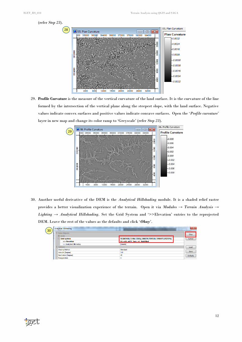
29. Profile Curvature is the measure of the vertical curvature of the land surface. It is the curvature of the line

formed by the intersection of the vertical plane along the steepest slope, with the land surface. Negative

values indicate convex surfaces and positive values indicate concave surfaces. Open the ‘Profile curvature’

layer in new map and change its color ramp to ‘Greyscale’ (refer Step 23).

30. Another useful derivative of the DEM is the Analytical Hillshading module. It is a shaded relief raster

provides a better visualization experience of the terrain. Open it via Modules → Terrain Analysis →

Lighting → Analytical Hillshading. Set the Grid System and ‘>>Elevation’ entries to the reprojected

DEM. Leave the rest of the values as the defaults and click ‘Okay’.

28

29

30


13

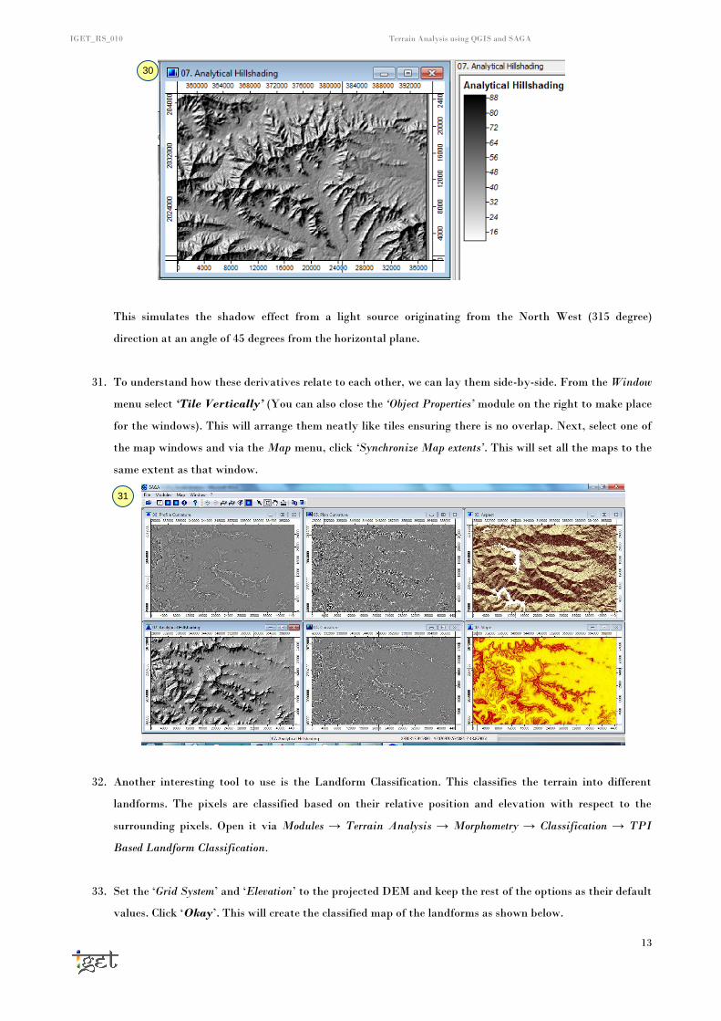
This simulates the shadow effect from a light source originating from the North West (315 degree)

direction at an angle of 45 degrees from the horizontal plane.

31. To understand how these derivatives relate to each other, we can lay them side-by-side. From the Window

menu select ‘Tile Vertically’ (You can also close the ‘Object Properties’ module on the right to make place

for the windows). This will arrange them neatly like tiles ensuring there is no overlap. Next, select one of

the map windows and via the Map menu, click ‘Synchronize Map extents’. This will set all the maps to the

same extent as that window.

32. Another interesting tool to use is the Landform Classification. This classifies the terrain into different

landforms. The pixels are classified based on their relative position and elevation with respect to the

surrounding pixels. Open it via Modules → Terrain Analysis → Morphometry → Classification → TPI

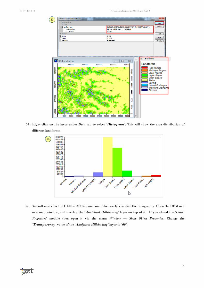
Based Landform Classification.

33. Set the ‘Grid System’ and ‘Elevation’ to the projected DEM and keep the rest of the options as their default

values. Click ‘Okay’. This will create the classified map of the landforms as shown below.

31

30


14

34. Right-click on the layer under Data tab to select ‘Histogram’. This will show the area distribution of

different landforms.

35. We will now view the DEM in 3D to more comprehensively visualize the topography. Open the DEM in a

new map window, and overlay the ‘Analytical Hillshading’ layer on top of it. If you closed the ‘Object

Properties’ module then open it via the menu Window → Show Object Properties. Change the

‘Transparency’ value of the ‘Analytical Hillshading’ layer to ‘60’.

33

34


15

36. Select the map window and click the ‘Show 3D View’ button. Set the ‘Grid System’ and

‘>>Elevation’ to the projected DEM layer. Click ‘Okay’. This will open the layer in the 3D-view window.

37. Click and drag the image. It will rotate around an axis in the direction in which you pull it. The controls

for the viewing angle and distance can be found in the tool bar above. Play around with these controls to

get used to handling the layer ( place the mouse cursor over each one to see what each one does).

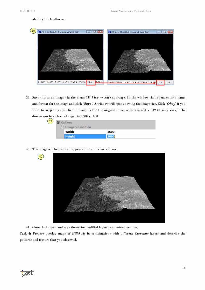
38. You might find that if you look at the terrain from a lateral view, it appears slightly flat. It makes it more

difficult to make out the elevation differences. To fix this, use the F1 and F2 keys to decrease or increase

the exaggeration of the terrain. An image when viewed with some exaggeration can make it easier to

35

36

37


16

identify the landforms.

39. Save this as an image via the menu 3D View → Save as Image. In the window that opens enter a name

and format for the image and click ‘Save’. A window will open showing the image size. Click ‘Okay’ if you

want to keep this size. In the image below the original dimensions was 384 x 239 (it may vary). The

dimensions have been changed to 1600 x 1000

40. The image will be just as it appears in the 3d View window.

41. Close the Project and save the entire modified layers in a desired location.

Task 4: Prepare overlay maps of Hillshade in combinations with different Curvature layers and describe the

patterns and feature that you observed.

38

39

40

terrain analysis - dst igetdst-iget.in/tutorials/iget_rs_010/iget_rs_010_terrain analysis.pdf ·...

Documents