term structures of credit spreads with incomplete accounting information darrell duffie and david...

Term Structures of Credit Spreads with Incomplete Accounting Information

Darrell Duffie and David LandoEconometrica, Vol.69, No. 3, (2001)

Presenter： d96723010 顏汝芳Nov. 21.2008

I. IntroductionI. Introduction

II. The Model II. The Model

III. ExtensionsIII. Extensions

Agenda

IV. ConclusionIV. Conclusion

I. IntroductionI. Introduction - Literature Review

- Motivation

- Contribution

Literature Review

Black and Scholes (1973) and Merton (1974) Black and Cox (1976) Geske (1977) Longstaff and Schwartz (1995) Leland (1994) Leland and Toft (1996) Anderson and Sundaresan(1996) Collin-Dufresne and Goldstein(2001) Zhou(2001)

Black and Scholes (1973) and Merton (1974)• A leading paradigm in corporate-bond valuation has taken

as given the dynamics of the assets of the issuing firm, and priced corporate bonds as contingent claims on the assets.

Black and Cox (1976) • Study the effects of bond indenture provisions.

Geske (1977) • Generalizations treat coupon bonds as compound options.

Longstaff and Schwartz (1995)• Incorporates both default and interest rates risk.

Collin-Dufresne and Goldstein(2001) Extend L-S in generating mean-reverting leverage ratios.

Literature Review (details)

The second-generation models allow for endogenous default, optimally triggered by equity owners whenassets fall to a sufficiently low level.

Leland (1994)• By introducing bankruptcy costs and tax effects to derive t

he close form of perpetual corporate bond. Leland and Toft (1996)

• The tax advantage of debt must be balanced against bankruptcy and agency costs in determining the optimal maturity of the capital structure.

Anderson and Sundaresan(1996)• Construct a dynamic non-cooperative game to determine e

ndogenously the firm’s reorganization boundary.

Literature Review (details)

Literature Review

The figure explain the term structure of credit spreads for varying asset volatilities.

Yield spreads for relatively risky firms would eventually climb rapidly with maturity.

Such severe variation in the shape of the term structure of yield spreads is uncommon in practice

This is Figure 2 in Giesecke (2004).

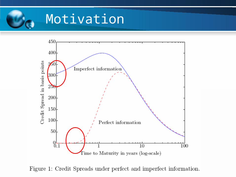
Motivation

In practice, it is typically difficult for investors in the secondary market for corporate bonds to observe a firm's assets directly, because of noisy or delayed accounting reports, or barriers to monitoring by other means.

Investors must instead draw inference from the available accounting data and from other publicly available information.

Under informational assumptions, we derive public investors' conditional distribution of the issuer's assets, explicitly accounting for the implications of imperfect information and survivorship.

With perfect information, yield spreads for surviving firms are zero at maturity, and are relatively small for small maturities, regardless of the riskiness of the firm.

With imperfect information, yield spreads are strictly positive at zero maturity because investors' are uncertain about the nearness of current assets to the trigger level at which the firm would declare default. This uncertainty causes a more moderate variation in spreads with maturity.

The shape of the term structure of credit spreads may indeed play a useful empirical role in estimating the degree of transparency of a firm.

Motivation

Motivation

With imperfect information, this paper have

mainly two important results as follows:

Bound short spreads away from zero with imperfect information.

Present a first example of a structural model

that is consistent with such a reduced-form representation.

Contributions

Contributions

The structural models described above link default explicitly to the first time that assets fall below a certain level.

As opposed to it, a more recent literature has adopted a reduced-form approach, assuming that the default arrival intensity exists, and formulating it directly as a function of latent state variables or predictors of default, see Duffee (1999).

The existence of a default intensity, moreover, is consistent with the fact that bond prices often drop precipitously at or around the time of default.

Contributions

Bounding short spreads away from zero can also be obtained in a structural model in which the assets of a firm are perfectly observable and given by a jump-diffusion process, as in Zhou (2001).

This approach is not, however, consistent with a stochastic intensity for default. Hence, this approach does not lay the theoretical groundwork for hazard-rate based estimation of default intensities.

One could, of course, build a model for a firm with complete information in which various different state variables determine the dynamics of assets or liabilities, and would therefore also be determinants of default risk.

II. The ModelII. The Model - Perfect information

- Imperfect information

- Default intensity

- Credit spreads

- Default-swap spreads

The model

First, the authors solve for the optimal capital structure and default policy.

given perfect information

Then derive the conditional distribution of the firm's assets, given incomplete accounting information, along with the associated default probabilities, default arrival intensity, and credit spreads.

given imperfect information

We begin by reviewing a standard model of a firm's assets, capital structure, and optimal liquidation policy. With some exceptions, the results are basically those of Leland and Toft (1996).

Perfect information (1/6)

The stochastic process V describing the stock of assets of our given firm is modeled as a geometric Brownian motion, which is defined on a probability space . We let Vt=eZ(t), where Zt=Z0+mt+σWt and m=μ- σ2/2.

• The firm generates cash flow at the rate δVt at time t, for some constant 0<δ<∞.

The firm issues debt so as to take advantage of the tax shields at the constant tax rate 0<θ<1. In order to stay in a simple time-homogeneous setting, the debt is modeled as a consol bond with total coupon rate C > 0.

• The tax benefits for this bond are therefore received at the constant rate θC, until liquidation.

The firm is operated by its equity owners, who are completely informed at all times of the firm's assets. This means that they have the information filtration (Ft) generated by V . The expected present value at time t of the cash flows to be generated by the assets, excluding the effects of liquidation losses and tax shields, conditional on the current level Vt of assets, is

(1)

A liquidation policy is an (Ft)-stopping time τ: Ω [0, ∞]. Given an asset level at liquidation of Vτ ; At the chosen liquidation time τ , a fraction 0<α<1 of the assets are lost as a frictional cost. The value of the remaining assets, ,

is, by an assumption of strict priority, assigned to debtholders.


The initial value of equity to shareholders, given a liquidation policy τ and coupon rate C, is

(2)

Equity shareholders would therefore choose the liquidation policy solving the optimization problem

(3)

The optimal liquidation time, as shown in Leland(1994), is the first time that the asset level falls to some sufficiently low boundary VB >0.


One conjectures that the optimal equity value at time t

is given by St = w(Vt) , where w solves the ODE

with the boundary conditions

and


Smooth-pasting condition


The stock price is solved, for ,

,

where

VB = . The associated expected present value of the cash flows to th

e bond at any time t before liquidation, conditional on Vt is

P 1-P


It is easy to check the optimality property

We suppose that the total coupon rate C*(V0) of the bonds to

be issued is chosen so as to maximize over C the total initial firm valuation,

which is the initial value of equity plus the sale value of debt.

From the procedure above, we can solve out the optimal capital structure and optimal liquidation policy.

Imperfect information (1/11)

Now we turn to how the secondary-market assesses the firm's credit risk and values its bonds.

While they do understand that optimizing equity owners will force liquidation when assets fall to VB, bond investors can NOT observe the asset process V directly.

Instead, they receive imperfect information at selected times t1, t2, …, with ti < ti+1. We assume that at each observation time t there is a noisy accounting report of assets, given by . And suppose that , where U(t) is normally distributed and independent of Z(t).

Also observed at each t is whether the equity owners have liquidated the firm.


That is, the information filtration (Ht) available to the secondary market is defined by

for the largest n such that tn ≦ t, where . For simplicity, we suppose that equity is not traded on the

public market to avoid complex asymmetric information.

Our main objective for the remainder of this subsection is to compute the conditional distribution of Vt given Ht .

We will begin with the simple case of having observed a single noisy observation at time t = t1.


In the procedure, we will need four main conditional density of logV(t)= Z(t) given different condition, they are respectively

Moreover, we have to know that

– The density of Yt is

– The density of Zt is

– The density of Ut is

The standard deviation of Ut may be thought of as a measure of the degree of accounting noise.


Claim : the density of Zt, conditional on

the noisy observation Yt and on τ > t. From the application of Bayes’ Rule,

Denote as the joint density of Zt and τ > t

conditional on the observation Yt = Zt + Ut. That is,

= , then we have


As an intermediate calculation, we need the conditional probability which is defined as follows

From the density of the first-passage time recorded in Chapter 1 of Harrison (1985), and from Bayes’ Rule, one obtains that


Then we can calculate the joint conditional density b(.)

using the definition of and Bayes’ Rule,

Finally, a calculation of the integral in with

Given survival to t, this gives us the conditional distribution of assets Vt with x = log v given Ht.


Suppose that Ut has expectation such that

implying an imperfect but unbiased accounting report.

We suppose that a noise-free asset report of

Our base case is = 10 % and the default boundary is 78.


Figure 2.– Conditional density for varying accounting precision.

86.3


Figure 3.– Conditional asset density, varying previous year asset level.


We also compute the Ht -conditional probability p(t, s) of survival to some future time s > t. That is,

For τ > t, we have

where


Figure 4.– Default probability, varying accounting precision.

Perfect inform.

Default intensity (1/5)

In the case of perfect information, that is, for a filtration such as (Ft ) to which Z is adapted, on the event that τ > t we have

It is tempting to conclude that the same is true with imperfect information, because

However, the integral itself does NOT converge to 0 as h goes to 0.


In this section, we prove that (in general) a non-zero limit exists, we give an explicit expression for the limit, and we show that this limit is in fact the intensity of τ.

The default stopping time has an intensity process λ with respect to the filtration (Ht) if λ is a non-negative progressively measurable process satisfying for all t, such that is an (Ht)-marti.

The intuitive meaning of the intensity is that it gives a local default rate, in that


Heuristics:


Figure 6.– Default intensity, varying accounting precision.


Figure 7.– Default intensity, varying previous year asset level.

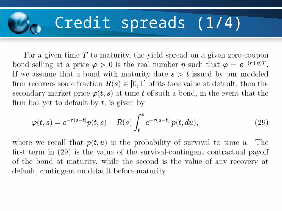
Credit spreads (1/4)


• Suppose that and it is easy to show that

is concave. It follows by Jensen‘s Inequality that yield spreads are larger at an outcome for that is conditionally unbiased for than they would be in the case of perfect information. Bond price 低 yield spread 大

• This is analogous to the fact that, in a Black-Scholes setting, the equity price as a function of asset level is increasing in the volatility of assets, and therefore the debt price is decreasing in asset volatility.

• One might extrapolate to practical settings and anticipate that, other things equal, secondary-market yield spreads are decreasing in the degree of transparency of a firm.公司越透明 (a 越小 ) yield spreads 小


Figure 8.– Credit spreads for varying accounting precision.

a = 0.00


Figure 9.– Credit spreads for varying previous year asset level.

V0 PD Credit spread

Default-swap spreads

Figure 10.– Default swap spreads with perfect and imperfect information. Base case.

III. ExtensionsIII. Extensions

Extensions (1/4)

This section outlines some extensions of the basic model. First, we allow for inference regarding the distribution of assets from several variables correlated with asset value, or from more than one period of accounting reports.

We briefly discuss how to model re-capitalization, or decisions by the firm that may be triggered by more than one state variable, such as a stochastic liquidation boundary.

We characterize the default intensity for cases in which the asset process V is a general diffusion process, with a general observation scheme.

Extensions (2/4)

Extensions (3/4)

Extensions (4/4)

IV. ConclusionIV. Conclusion

Conclusion

We suppose that bond investors CANNOT observe the issuer’s assets directly, and receive instead only periodic and imperfect accounting reports to study the implications of imperfect information for term structures of credit spread on corporate bonds.

Contrary to the perfect-information case, there exists a default-arrival intensity process.

Bound short spreads away from zero with imperfect information.

Thanks sincerely

for listening and advising

term structures of credit spreads with incomplete accounting information darrell duffie and david...

Documents