-ter of on children ever born and children surviving · dead among the children ever borne by a...

-ter 111

ES)TIMATION OF CHILD MORTALITY FROM INFORMATION ON CHILDREN EVER BORN AND CHILDREN SURVIVING

A. BACKGROUND OF METHODS Brass found that the relation between the proportion of children dead, D(i), and a life-table mortality meas-

1. Use of&ta on child survivorship ure, q ( x ) , is primarily influenced by the age pattern of It is well known that the proportions of children ever fertility, because it is this pattern that determines the dis-

born who have died are indicators of child mortality and tribution of the children of a group of women by length can yield robust estimates of childhood mortality. The of exposure to the risk of dying. He developed a set of births to a group of women follow some distribution multipliers to convert observed values of D(i) into esti- over time, and the time since birth is the length of expo- mates of q(x ), the multipliers being selected according sure to the risk of dying of each person. The proportion to the value of P(I)/P(2)-a good indicator of fertility dead among the children ever borne by a group of conditions at younger ages-where P(i) is the average women will therefore depend upon the distribution of parity or average number of children ever born reported the children by length of exposure to the risk of dying by women in age group i . Brass estimated the k(i) mul- (that is, upon the distribution in time of the births) and tipliers by using a third-degree polynomial of fixed upon the mortality risks themselves. BY allowing for the shape but variable age location to represent fertility? the effects of the distribution of the births in time, such a togit system generated by the general standard (see proportion of dead children can be converted into a chapter I, subsection B.4) to provide the mortality ele- conventional mortality measure expressing their average ment, and a growth rate of 2 per cent per annum to gen- experience. Specifically, the proportions of children erate a stable age distribution for females. dead claSSified the mother's five-~ear age group Or An important =umption made in the development of duntion of mamag provide estimates of the proC this method is that the risk of dying of a child is a func- abilities of betwen birth and various tion only of the age of the child and not of other factors, In certain culturn to be such as mother's age or the child's birth order. In prac- likely to Of mamabe than to give tice, it appears that children of young mothers experi- comet infomation about 'ge* x, the estimation ence momlity risks well above average. For this r e a m pmadure On data by mar- the estimate of the infant mortality rate p(l) (the proba-

be prefemd' However' the use Of data bility of dying before age 1) that can be derived from classified by duration is not recommended in countries of aged 15-19 fmluently susesk heavier where oonsemua' unions am 'quent and mhtivel~ child momlity than derived from mpoa of unstable. older women. Therefore, mortality estimates based on

Bras' was the first to a prwedur con- the reports of women aged 15-19 are generally disre- verting proportions dead children ever born =ported garded, in part for this reason and in part because the by in age groups 20-249 etc. into estimates numbers of children born and dead are usually small. of the probability of dying before attaining certain exact c ~ l d h d ages. ~ ~ l l ~ ~ i ~ ~ the nomtion in he litenam Trying to increase the flexibility of Brass* original and dng the symbol D ( ~ ) to denote the method. Sullivan' computed another set of multipliers dead among children ever born to women in succesive by using least-quares regression to fit equation (A.0 to five-year age (where = 1 aignifia age group data generated from observed fertilit schedules and the Y 15-19: i = 2 denotes 2044; etc.), B~~ developed a pro- Coale-Demeny life tables? Trussell estimated a third cedure to convert D(i ) values into estimates of q(x ), set of multipliers by the same means but using data gen- where q(x)= l . ~ - l ( ~ ) , the probability of dying erated from the model fertility schedules developed by between birth and exact age x. The basic form of the estimation equation proposed by Brass is William Brass Merirodsfir fitlmatin Fertility and Momlity fmm

United and lkjktive h a (Chapel tiiff, North Carolina. Carolina

q(x)= k(i) D(i) Po ulrtion Center, Laboratories for Population Statistics, 1975). ( I ) rJermiah M. Sullivan. "Models for the estimation of the pmbabili-

ty of dying between birth and exact ages of early childhood '. Popula- where the multiplier k (i ) is meant to adjust for non- tion Studies. vol. XXVI. No. I (Mach 1972). pp. 79-97.

mortality factors determining the value of D(i ). ' Ansley J. Coale and Paul Demeny. R e g i o ~ l Model Li/c Tables and Stabfe Popukr~ioonr (Princeton. New Jeney. Princeton University Press 1966).

I William Brass. "Uses ofcensus or survey data for the estimation of T. lames Tnrsseli. "A R-estimation of the multiplying factors for vital ntes" (E/CN.14/CAS.4/V57), aper prc arcd for the African the Brass technique for determining childhood survivorshi rates". Seminar on Vital Statistics, ~ d d i s ~ b a g a . 14- 19 becember 1964. Population Sfudies, vol. XXIX. No. I (March 1975). pp. 97-10!.

73

Coale and ~russell! The general theow on which these methods are based is eskntiallv the'same. but thev arrive at somewhat different r n ~ l t ~ ~ l i e r s because the dati bases used in each case are different. Since the Sullivan variant has no obvious advantages over that proposed by Trussell. whereas the latter is based on a wider range of cases, the Trussell procedure is described here. It must be mentioned, however, that the multipliers presented are a more recent and more satisfactory version of those originally proposed by Trussell in 1975.

It is important to take note that this method of estimation is based on the assumption that fertility and childhood mortality have remained constant in the recent past. If, for example, fertility has been changing, the ratios of average parities obtained from a cross-sectional survey will not replicate accurately the experience of any cohort of women and will not provide a good ~ndex of the distribution in time of the births to the women of each age group.

The problems caused by declining fertility can be avoided when data for true cohorts are available (from censuses or surveys taken five or 10 years apart). In this case, an estimation method specifically designed for cohorts experiencing fertility change should be used?

Preston and ~alloni' propose an alternative approach to estimate the time location of births, which circumvents all the problems associated with changing fertility. This approach is closely related to the "own-children" procedure for estimating fertility from an age distribution (see chapter VIII, section C). If it is possible to link, within households, the records of mothers and their surviving children, it becomes possible to tabulate surviving children according both to their own age and to that of their mothers. Given an age pattern of mortality, say, from one of the Coale-Demeny regional model life tables, the combination of the proportion of children dead and the age distribution of the surviving children of women from some particular age group uniquely determines a level of mortality. The age distribution of surviving children is used to define the age distribution of children ever born without recourse to fertility models. In an actual application, the choice between the age distribution of surviving children and the ratio of consecutive parities to estimate the real distribution of births over time, depends upon data availability and upon a rough assessment of the likelihood each approach has of yielding the best possible estimate. In cases where age-reporting is good and most children live with their mothers, the approach suggested by Preston and Palloni may be the better, particularly if fertility is changing. In cases where age-reporting or completeness of enumeration is poor, or where a sizeable proportion

Ansley J. Coale and T. James Trussell, "Model fertility schedules: variations in the age structure of childbearing in human populations". Po ulorion Index, vol. 40. No. 2 (April 1974). pp. 185-258.

'Phis method is presented in r t i o n E and it uses the estimation equations and coefficients given in tables 70-7 1. ' Ssmuel H. Preston and Alberto Palloni, "Fine-tuning Brass-ty mortalit estimates with data on a ea of surviving children". PoPuE 6on d c r i w o the United Nations, k 104977 (United Nations publi- 1$ cation, Sala o. E.78.Xl11.6). pp. 72-87.

of children do not live with their mothers or cannot be properly linked to them because of poor information, the parity-ratio approach is very likely to be better. A detailed description of the Preston-Palloni method is not included here, in part because in most cases where mortality needs to be estimated indirectly, age distributions are at best only moderately reliable, and in part because the data required for its application are not as widely available as the proportions of children dead. However, the user who has access to the former data for cases where biases due to fertility change may be a problem is encouraged to consider the application of this method.

Probably a more widespread problem is posed by declining mortality. The procedures outlined above all assume that a constant pattern and level of mortality have prevailed in the recent past of the population under study. In most countries, however, mortality has been declining.

~ e e n e ~ ~ was the first to examine the effects of changing mortality on the performance of the child-mortality estimation procedure. Using infant mortality as an index of mortality level in a one-parameter logit life- table system, he calculated the proportions of children dead that would be observed if infant mortality were changing linearly through time. On the basis of these simulated cases, he showed that for plausible annual rates of change in infant mortality, the q(1) values estimated from data on children ever born and surviving for different age groups of mother could be matched with the q(1) values prevalent during a set of years before the survey; and that this set of years was, for all practical purposes, invariant with respect to the rate of mortality change. Using this empirical finding, Feeney developed an estimation procedure to establish the set of years to which infant mortality rates estimated from data on children ever born and children surviving refer. This procedure was developed from data generated by using a one-parameter logit life-table system derived from the general standard (see cha ter 1, subsection B.4) and the Brass fertility The use of g(l), infant mortality, as an indicator of mortality level and as the estimated parameter makes the underlying age pattern of mortality important to the results, since similar overall levels of mortality (life tables with the same expectation of life at birth, for example) can be associated with markedly different infant mortality rates. As a result, the Feeney method is likely to yield biased q(1) estimates when the mortality pattern in early childhood of the population under study does not resemble that embodied 'by the general standard. For this reason, Feeney's original method is not described in detail.

It is fairly straightforward to apply Feeney's approach to data generated with other mortality models. Coale

Griffith Feeney. "Estimating infant mortality rates from child survivorship data by age of mother". Asian and Pacc Census Neu~Ie~ler. vol. 3. No. 2 (November 1976). p. 12-16: and &fith Feene . "Er timating infant mortalit trends %m child survivorship dutr". b@u- lion Srudies, vol. XXXIJ, No. I (March 1980). p p 109-128.

lo W. Brass. Mc~hads/or fiiimaaring FcrtiIity and Morroli!r fkq~ Lima; ired and Drfitiw &fa.

and ~russell" carried out this exercise by assuming that period mortality changes can be modelled as movements through successively higher (or lower) levels of a set of model life tables, so that cohort life tables may be obtained by chaining together the mortality rates experienced by true cohorts living through the different periods. In this case, it can also be shown empirically that the child mortality estimate of the Brass type obtained from data for women in age group i , for example, is equal to the corresponding value prevalent during some particular period t ( x ) years before the survey, and that this period is, for most practical purposes, invariant with respect to the speed of mortality change, so long as the rate of change is roughly constant over time. Because these time-location estimates have been derived in a manner that is consistent with that used in deriving the Trussell multiplying factors employed in estimating child mortality in this chapter, this timing procedure is described here.

An alternative solution to the problem of declining mortality is possible if data on children ever born and surviving are available from two surveys taken five or 10 years apart. It arises, once again, from the use of a hypothetical cohort representing the intersurvey experience; and it provides mortality estimates that refer to the intersurvey period. This estimation approach is not sen- sitive to the exact shape of mortality changes, but changes in the completeness of reporting of dead children from one survey to the next or population changes that are selective for the number of dead children may seriously affect the results.

To conclude these preliminary remarks on the methods presented in this chapter, it should be pointed out that for several of them two variants are presented: one variant to be applied when data on children ever born and surviving are classified by age of mother; and another when they are classified by duration of first marriage. The variants based on data classified by duration of marriage are, strictly speaking, based on the assumption that women, once mamed, stay mamed until age 50 (the assumed upper limit of the potential reproductive life of a woman). Therefore, the duration-based methods should strictly be applied only to data from currently mamed women still in their first union. How- ever, in practice, no serious biases will arise when they are applied to data pertaining to all ever-married women, as long as their marriage duration is calculated as the time elapsed since first marriage.

As a last word of caution, it must be said that the performance of the duration variants of these methods can be rather poor when "duration" is not accurately measured. Problems in the measurement of this variable have been described in chapter 11, subsection A.2, and are only briefly cited now. Duration of marriage is defined as the time elapsed since first union, regardless of whether that union is legal. Data on duration of mar-

I 1 Ansley J . Coale and James Trussell. "Estimating the time to which Brass estimates apply". annex I to Samuel H. Preston and Al- berto Palloni. "Fine-tuning Brass-type mortality estimates with data on ages of surviving children", Population Bulletin of the United Na- tions, No. 10-1977, pp 87-89.

riage will be less than ideal when only legal unions are considered; when the time elapsed is not measured from the beginning of the first union, but rather from that of the current union; or when, as in some Muslim cultures, the entrance into a legal mamage predates the initiation of cohabitation. In populations where these problems are likely to arise, the duration variant should not be used.

2. Organization of this chapter All the estimation procedures presented in this

chapter have one characteristic in common: they use data on children ever born and surviving. However, the methods can be separated into categories according to the exact type of data they require (whether classified by age or by duration of mamage, for example), or according to the practical constraints that their assumptions impose (whether fertility is assumed to be constant or not). Sections B-E are devoted to the different categories. To aid the user in selecting that most suited for a particular application, brief descriptions of each section follow (see also table 46):

Section B. Erlimation of child mortality using &ta clars~jied by age. In this section, the most recent version of the original Brass estimation procedure is presented (Trussell's method). Estimates of q(2), q(3). q(5). q(10). q(15) and q(20), as well as of the periods to which they refer in cases where a smooth change in mortality can be assumed, are obtained from data on children ever born and surviving classified by age of mother. Fertility patterns are assumed to remain constant;

Section C. Ertimation of child mortality wing &la clarsijied by duration of -age. In this section, a variant of the original Brass method that may be applied to data classified by duration of first marriage is presented. Esti- mates ofq(21, q(3), q(5). q(10), q(15), q(20) and q(251, as .well as of the periods to which they refer in cases where a smooth change in mortality can be assumed, are obtained from data on children ever born and surviving classified by the mother's marriage duration. Marital fertility patterns are assumed to remain constant;

M i o n D. Ertimation of intersumy child mortality using &fa for a hypothetical intersurvey cohort. In this section, data from two censuses or surveys five years apart are used to estimate average intersurvey child mortality. The use of hypothetical cohorts circumvents the neces- sity of assuming that fertility and mortality have remained constant. Therefore, if the data at the two points in time considered are similar in quality and moderately reliable, intersurvey estimates are to be preferred over those derived by other means;

Section E Estimation of child mortality when the fertility exwence of true cohorts is known. In this section, data from two censuses or surveys five or 10 years apart are used to determine the parity ratios for true cohorts; and these ratios, in turn, are employed in estimating child mortality from data collected by the second census or survey. Both an age and a duration variant are described in subsection E.2. The time location of the child mortality estimates obtained is also estimated and constant fertility is not assumed.

T M L E ~ ~ . SCHEMATIC GUIDE TO CONTENTS OF CHAPTER 11 1

SlcIba

B. Estimation of child mortality rates using data classified by age (one SUN^)')

C. Estimation of child mortality using data classified by duration of marriage (one survey)

D. Estimation of intersurvey child mortality using data for a hypothetical intersurvey cohort (data by age from two surveys five years apart)

E. Estimation of child mortality when the fertility experience of true cohorts is known

Wo/~gu* Children ever born classified by

five-year age group of mother Children surviving (or dead)

classified by five-year age group of mother

Women classified by five-year age group

Children ever born classified by five-year duration of marriage group of mother

Children surviving (or dead) classified by five-year duration of marriage group of mother

Ever-married women classified by five-year duration of marriage group

Children ever born classified by five-year age group of mother from two surveys or censuses five years apart

Children surviving (or dead) classified by five-year age group of mother from two surveys or censuses five years apart

Women classified by five-year age group from two surveys or censuses five years apart

Children ever born classified by five-year age (duration) group of mother from surveys or censuses five or I0 years apart

Children surviving (or dead) classified by five-year age (duration) group of mother from the second survey or census

Women (ever-married women) classified by five-year age (duration) group

B. ESTIMATION OF CHILD MORTALITY RATES USING DATA CLASSIFIED BY AGE

The data required for this method are listed below: (a ) The number of children ever born, classified by

sex (see note) and by five-year age group of mother; (b) The number of children surviving (or the number

dead), classified by sex (see note) and by five-year age group of mother;

(c) The total number of women (irrespective of marital status), classified by five-year age group. Note that all women, not merely ever-mamed women, must be considered.

Note should be taken also that classification by sex for

-ycnmr q(2). q(3). q(5). q( 10). q( 15) and

q (20) Reference period for each q(x)

estimate

q(2). q(3). q(S). q(10). q(l5). q(20) and q(25)

Reference period for each q(x) estimate

Intersurvey estimates of q(2). q(3). q(5). q(10). q(15) and q(20)

q(2). q(3). q(5) and q( 10). and their time reference periods when data are classified by age and surveys are five years apart

q(3). q(5) and q(10) with reference periods when data are classified by age and surveys are 10 years apart

q(3). q(5) and q(10) with reference penods when data are classified by duration and surveys are five years apart

q(5) and q(10) with reference periods when data are classified by duration and surveys are 10 years apart

children ever born and surviving is desirable, not essen- tial. If it is available, child mortality for each sex can be estimated separately; whereas if it is not available, estimates for each sex can only be obtained by assuming that the sex differentials in the population being studied are the same as those embodied by model life tables whose mortality level is consistent with the estimated child mortality of both sexes, or by making some other assumption about the relationship between male and female child mortality.

When data on children ever born are classified by sex, their consistency may be ascertained by computing the sex ratios (defined as the average number of male children per female child) of children ever born by age of mother. Ideally, these sex ratios should not vary sys- tematically with age and their values should be between

1.02 and 1.07. Studies made in countries when birth regiitration is fairly complete have shown that the sex ratio at birth is remarkably constant and that its usual value is around 1.05 males per female. In populations originating in Africa south of the Sahara, this value appears to be closer to 1.03. In either case, however, its constancy and the fact that women are supposed to declare all the children they have ever borne alive, whether these children survived or not, allows a simple consistency check. In populations other than those originating in sub-Saharan Africa, sex ratios higher than 1.07 or lower than 1.02 suggest differential omission of females or males, respectively, or misreporting of the sex of the reported children.

2. Computationalprocedure The steps of the computational procedure are

described below. Step 1: calculation of awmge parity per wman. Parity

P(1) refers to age group 15- 19, P(2) to 20-24 and P(3) to 25-29. In general,

where CEB(i) denotes the number of children ever borne by women in age group i ; and FP(i) is the total

number of women in age group i , irrespective of their marital status. Recall that, following the usual conven- tion, variable i refers to the different five-year age groups considered. Thus, the value i = 1 represents age group 15-19, i = 2 group 20-24 and so on. The treat- ment of women whose parity is not stated is discussed in chapter 11, subsection A.2, and annex 11. In general, if the El-Badry technique for estimating w e non-response cannot be applied, women of unstated parity should be included in the female population denominator when calculating average parity, since childless women are often misclassified as cases of non-response.

Step 2: calcuIation ofproportion of childnn de4d fw each age group of mother. The propol-tion of children dead, D(i), is defined as the ratio of reported children dead to reported children ever born, that is,

where CEB(i ) is defined as in step 1 ; and CD(i ) is the number of children dead reported by women in age group i .

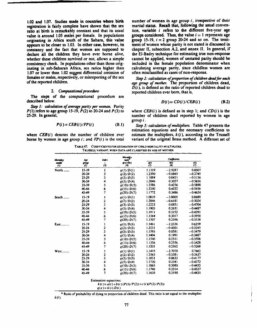
Step 3: calculation of muItipIiers. Table 47 presents the estimation equations and the necessary coefficients to estimate the multipliers, k(i), according to the Trussell variant of the original Brass method. A different set of

TABLE^^. COEFFICIENTS FOR ESTIMATION OF CHILD MORTALITY MULTIPLIERS. TRUSSELL VARIANT. WHEN DATA ARE CLASSIFIED BY AGE OF MOTHER

North ....... 15-19 20-24 25-29 30-34 35-39 40-44 45-49

South ....... 15-19 20-24 25-29 30-34 35-39 4-44 45-49

East ....... . . . 15-19 20-24 25-29 30-34 35-39 40-44 45-49

West ......... 15-19 20-24 25-29 30-34 35-39 40-44 45-49

Estimation equations: k ( i ) = a ( i ) + b ( i ) (P(I)lP(2))+cfi)(P(Z)lP(3))

' Ralio or probability of dying to proportion of children dead. This ratio is set equal to the multiplier k ( i ) .

coefficients is provided for each of the four different families of model life tables in the Coale-Demeny system.

Step 4: calculation o f p d d i l i t i e s 4dying and of surviving. Estimates of the probability of dying, q ( x ) , are obtained for different values of exact age x as the prod- uct of the reported proportions dead, D(i) , and the corresponding multipliers, k ( i ) . Note that the value of x is not generally equal to that of i , because x is related, in broad terms, to the average age of the children of women in age group i .

Once q ( x ) is estimated, its complement l ( x ) , the probability of surviving from birth to exact age x , is readily obtained as I(x ) = 1.0 -q (x ).

Step 5: calculation 4 mfemnce period. As explained

earlier, when mortality is changing smoothly, the reference period, t ( x ) , is an estimate of the number of years before the survey date to which the child mortality estimates, q ( x ) , obtained in the previous step refer. The value of t ( x ) is also estimated by means of an equation whose coefficients were estimated from simulated cases by using linear regression. The equation used in this case is presented in table 48 together with a set of values for its coefficients.

3. A detailed example The data shown in table 49 were gathered by a survey

carried out in Panama between August and October 1976. They are used to illustrate the method just described. However, before proceeding with the estimation of child mortality, a quick check of the consistency

TABLE^^. COEFFICIENTS FOR ESTIMATION OF THE REFERENCE PERIOD,I(X)~ TO WHICH THE VALUES OF Q(X) ESTIMATED FROM DATA CLASSIFIED BY AGE REFER

A@ I d x A@ Avmtu - C Q ~

77 i u~hwfe di) b(i) r(r) i;, (1) (3) (5) - (6) f 7) (8)

North ....... 15-19 I I q ( l ) 1.092 1 5.4732 - 1.9672 20-24 2 2 q ( 2 ) 1.3207 5.375 1 0.2 133 25-29 3 3 q ( 3 ) 1.5996 2.6268 4.3701 30-34 4 5 q ( s ) 2.0779 - 1.7908 9.4 126 35-39 5 10 q(1O) 2.7705 -7.3403 14.9352 40-44 6 IS q ( l s ) 4.1520 - 12.2448 19.2349 45-49 7 20 q(20) 6.%50 - 13.9160 19.9542

South ....... 15-19 I I q ( l ) 1 .O900 5.4443 -1.9721 20-24 2 2 9 0 ) 1.3079 5.5568 0.202 1 25-29 3 3 q ( 3 ) 1.5173 2.6755 4.747 1 30-34 4 5 q ( 5 ) 1.9399 -2.2739 10.3876 35-39 5 10 q(10) 2.6157 -8.4819 16.5153 40-44 6 15 q ( l s ) 4.0794 - 13.8308 21.1866 45-49 7 20 q(2O) 7.1796 - 15.3880 2 1.7892

East ...... .. .. 15-19 1 I q ( l ) 1.0959 5.5864 - 1.9949 20-24 2 2 q ( 2 ) 1.292 1 5.5897 0.363 1 25-29 3 3 q ( 3 ) 1 .SO2 1 2.4692 5.0927 30-34 4 5 q ( 5 ) 1.9347 -2.6419 10.8533 35-39 5 10 q( 10) 2.6197 -8.9693 17.098 1 4044 6 15 q ( l s ) 4.1317 - 14.3550 2 1.8247 45-49 7 20 q(20) 7.3657 - 15.8083 22.3005

West ......... 15-19 I I q ( l ) 1.0970 5.5628 - 1.9956 20-24 2 2 q ( 2 ) 1.3062 5.5677 0.2962 25-29 3 3 9 0 ) 1.5305 2.5528 4.8962 30-34 4 5 q ( 5 ) 1.999 1 -2.4261 10.4282 35-39 5 10 q(10) 2.7632 -8.4065 16.1787 4044 6 I5 q ( l 5 ) 4.3468 - 13.2436 20.1990 45-49 7 20 q(2O) 7.5242 - 14.2013 20.0 162

Estimation equation:

' Number of years prior to the survey.

TABLE@. CHILDREN EVER BORN AND CHILDREN SURVIVING. BY SEX AND AGE OF MOTHER. PANAMA. 1976

of the data presented is camed out by computing the sex ratios of the number of children ever born. Column (7) of table 49 shows these ratios. They are computed by dividing the number of male children ever born by the corresponding number of female children. As an example, for age group 20-24, the sex ratio is

and the overall sex ratio is

The sex ratios given in column (7) of table 49 fluctuate somewhat by age of mother but show no systematic trend, and the overall sex ratio is acceptably close to the expected value of 1.05. Furthermore, since some variation of the sex ratios by age is expected because of the relatively small sample being considered, it is concluded that this test shows no clear deficiency in the data.

Step I: calculation of m g e ponponty per woman. Aver- age parities P(1), P(2) and P(3) are calculated by dividing the number of children ever born of each sex (appearing in columns (3) and (5) of table 49) by the total number of women (column (2) of that table). Thus, for example, Pm (I), the mean number of male children ever borne by women aged 15- 19 is

The complete sets of Pm (i) and Pf (i) values are shown in columns (3) and (4) of table 50.

Note that the values of P(i) for both sexes combined are just the sum of Pm (i) and Pf (i), the mean number of male and female children, respectively, born to women of age group i .

TABLE 50. AVERAGE PARITY PER WOMAN, BY SEX OF CHILD AND AGE OF MOTHER. PANAMA, 1976

To calculate the D(i) values for both sexes combined, the deaths have to be added and then divided by the total number of children ever born (sum of males and females). Hence, D, (I) for both sexes would be

Table 51 shows a complete set of the proportions of children dead.

TABLE 5 1. PROFORTIONS OF CHILDREN DEAD. BY SEX OF CHILDREN AND AGE OF MOTHER. PANAMA. 1976

Step 3: calculation of mult@liers. The multipliers, k (i), required to adjust the reported proportion dead, D(i), for the effects of the age pattern of childbearing are calculated from the ratios P(l)/P(2) and P(2)/P(3), by using the equation and the coefficients listed in table 47. Thus,

It is assumed that the West family of model life tables is an adequate representation of mortality in Panama, so values of a(i), b(i) and c(i) are taken from the bottom panel of table 47. Given the values of P(l), P(2) and P(3) shown in table 50, values of k(i) can be calculated for each sex and for both sexes combined. The full set of k(i) values is shown in table 52. As an example, the multiplier for the male children of women aged 20-24 (i = 2) is

TABLE 52. TRUSSELLS MULTIPLIERS FOR CHILD MORTALITY ESTIMATION. WEsr MODEL; PANAMA. 1976

A& InLx M u f i ~ I m kfl) fa:

77 i mkJ F d Mua /2J /3J /4J /JJ

Step 2: calcularion of proporrion of chilbn d e d for each age group of mother. The values of this proportion, D(i), are computed from table 49 by dividing the number of children dead of each sex, given in columns (4) and (6), by the children ever born of the corresponding sex, shown in columns (3) and (5). Thus, Dm (I), the proportion of male children dead among those ever born to women aged 15- 19 is

Dm (I)= 24/278 = 0.0863. Step 4: calculation of probabjlities of dying and of mrviv-

TABLE 53. Emrum OP W O M B U m E S OP DYlNO AND OF WRVIVINO. BY SEX DERIVED FROM CHILD SURVIVAL DATA CLASSIFIED BY AOE OF MOTHPA, WBIT MODEL: PANAMA. 1976

ing. The estimated values of the probabilities of dying, q(x), are now calculated by multiplying the k ( i ) values appearing in table 52 by the corresponding proportions dead, D(i) , given in table 51. A complete set of q(x) estimates is shown in table 53. As an example, the value of qy (5) is obtained as follows:

Since every q(x) value is the probabilistic complement of the probability of surviving, I(x), the latter value can be obtained by subtracting the former from 1.0. Thus,

In table 53, every q(x) value is accompanied by its corresponding I(x ) value.

Step 5: calculation of reference period. Since mortality is not liely to have remained constant in Panama until 1976, it is useful to know the reference period, t(x), of each q ( x ) estimate. The values of the ratios P(l)lP(2) and P(2)/P(3) that are needed to estimate t (x) have already been computed in step 3. The form of the estimation equation and the values of the coefficients needed to estimate t(x) are obtained from table 48, again assuming a West mortality pattern. The value of r / (3) is calculated here as an example:

Thus, the estimated qf (3) value of 0.0595 is similar to that corresponding to the period life table in operation 4.24 years before the date of the survey, which may itself

be regarded as the average date of interview. Since the survey took place between August and October 1976, in rough terms ~ ( 3 ) refers to mid-1972. The complete set of estimated t (x ) values is presented in table 54.

Note that the t(x) values imply that the estimates of q(l), q(2), q(3) and q(5) obtained above refer to mortality conditions prevalent approximately one year, hvb and one-half years, four and one-half years and six and one-half years before the survey, respectively; thematter, the estimated values of t(x ) increase by some two and one-half to three years per age group. These values appear to be quite consistent with the notion that because the estimate of q(2), for example, is based mainly on information corresponding to women aged 20-24, whose childbearing experience is relatively recent, the q(2) estimate should also refer to the recent experience of the population. The plausibility and consistency of the values oft (x) is reassuring. They provide important information for the study of child mortality trends over time.

4. Comments on the &tailed example The calculation of the sex ratios of children ever born

by age group of mother did not reveal any irregularities that could not be explained by the small numbers involved in most cases. Another way to assess the quality of the data on children ever born is by examining the behaviour of the average parities reported by women of each age group. Unless fertility rose at some time in the past, average parities should increase with age up to age group 45-49. According to this rough test, data for Panama again appear to be satisfactory,. although the very small increase in parity from ages 40-44 to ages 45- 49 is somewhat suspicious (the average number of male children actually declines slightly). It is of interest to examine the parities because any omission of children

TABLE 54. ESTIMATES OF THE REFERENCE PERIOD' TO WHICH THE ESTIMATED PROBABILITIES OF DYING REFER. WEST MODEL; PANAMA. 1976

Number of years prior to the survey.

80

ever born might be made up disproportionately of dead children, thus greatly affecting the proportion dead. In the case in hand, the parity data show no clear evidence of omission. The proportions of dead children increase rapidly with age of mother, especially above age 35, if one ignores the value for women aged 15-19 (this value is almost always out of line with subsequent values, probably because the children of young women are, in fact, subject to higher mortality risks); these proportions thus give no indication of increasing omission of dead children as age rises. The very rapid increase in the proportions dead with age of mother suggests that a combination of effects is in operation: an increasingly longer average exposure to the risk of dying of the children and considerably higher child mortality from 10 to 15 years before the survey.

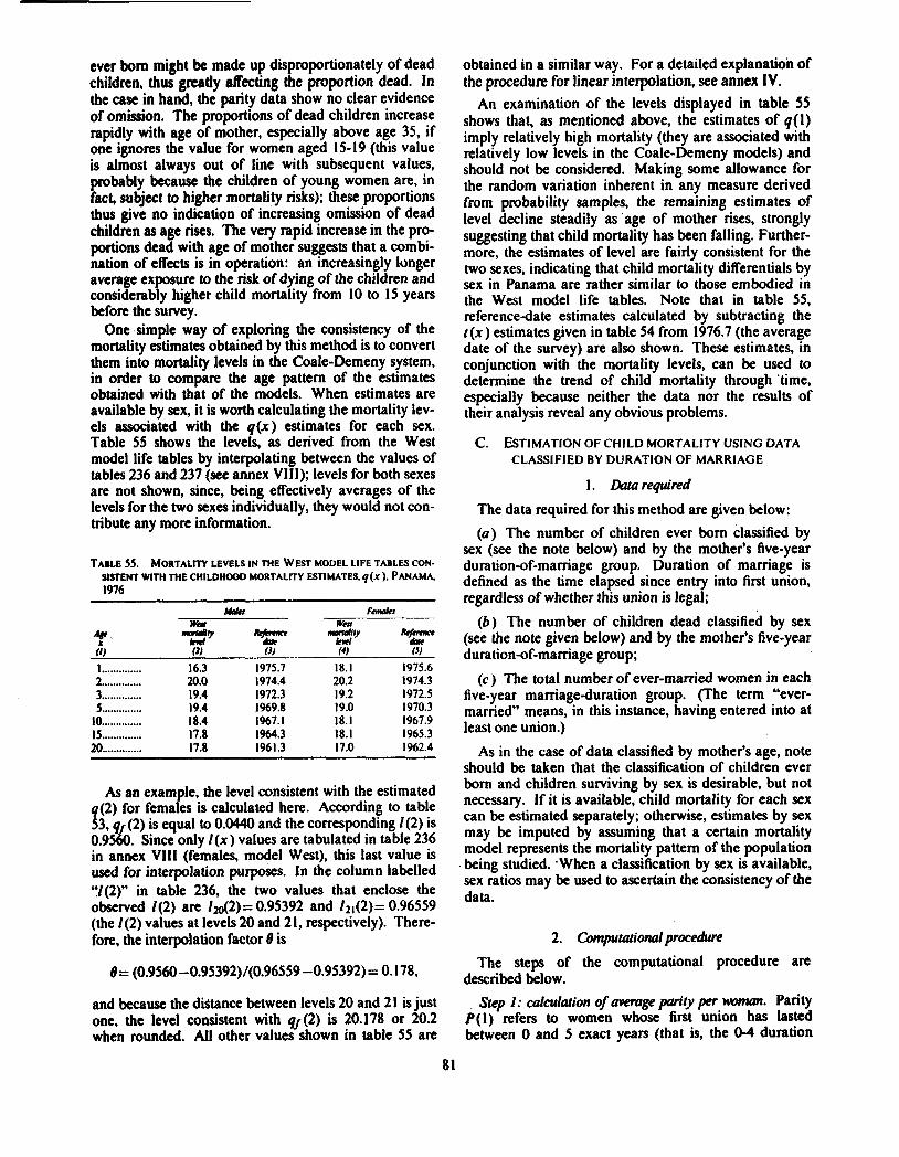
One simple way of exploring the consistency of the mortality estimates obtained by this method is to convert them into mortality levels in the Coale-Demeny system, in order to compare the age pattern of the estimates obtained with that of the models. When estimates are available by sex, it is worth calculating the mortality levels associated with the q(x) estimates for each sex. Table 55 shows the levels, as derived from the West model life tables by interpolating between the values of tables 236 and 237 (see annex VIII); levels for both sexes are not shown, since, being effectively averages of the levels for the two sexes individually, they would not con- tribute any more information.

TABLE 55. MORTALITY LEVELS IN THE WEST MODEL LIFE TABLES CON- SInENT WITH THE CHILDHOOD MORTALITY ESTIMATES. 9 ( ~ ) . PANAMA, 1976

As an example, the level consistent with the estimated q(2) for females is calculated here. According to table 53, (2) is equal to 0.0440 and the corresponding l(2) is 0.95 % . Since only l(x) values are tabulated in table 236 in annex VIlI (females, model West), this last value is used for interpolation purposes. In the column labelled 'tl(2)" in table 236, the two values that enclose the observed l(2) are 120(2)= 0.95392 and lZ1(2)= 0.96559 (the l(2) values at levels 20 and 2 1, respectively). There- fore, the interpolation factor 8 is

and because the distance between levels 20 and 2 1 is just one, the level consistent with qj(2) is 20.178 or 20.2 when rounded. All other values shown in table 55 are

obtained in a similar way. For a detailed explanation of the procedure for linear interpolation, see annex IV.

An examination of the levels displayed in table 55 shows that, as mentioned above, the estimates of g(l) imply relatively high mortality (they are associated with relatively low levels in the Coale-Demeny models) and should not be considered. Making some allowance for the random variation inherent in any measure derived from probability samples, the remaining estimates of level decline steadily as age of mother rises, strongly suggesting that child mortality has been falling. Further- more, the estimates of level are fairly consistent for the two sexes, indicating that child mortality differentials by sex in Panama are rather similar to those embodied in the West model life tables. Note that in table 55, referencedate estimates calculated by subtracting the r(x) estimates given in table 54 from 1976.7 (the average date of the survey) are also shown. These estimates, in conjunction with the mortality levels, can be used to determine the trend of child mortality through 'time, especially because neither the data nor the results of their analysis reveal any obvious problems.

C. ESTIMATION OF CHILD MORTALITY USING DATA CLASSIFIED BY DURATION OF MARRIAGE

The data required for this method are given below:

(a) The number of children ever born classified by sex (see the note below) and by the mother's five-year duration-of-mamage group. Duration of marriage is defined as the time elapsed since entry into first union, regardless of whether this union is legal;

(b) The number of children dead classified by sex (see the note given below) and by the mother's five-year duration-of-marriage group;

(c) The total number of ever-married women in each five-year mamageduration group. (The term "ever- married" means, in this instance, having entered into at least one union.)

As in the case of data classified by mother's age, note should be taken that the classification of children ever born and children surviving by sex is desirable, but not necessary. If it is available, child mortality for each sex can be estimated separately; otherwise, estimates by sex may be imputed by assuming that a certain mortality model represents the mortality pattern of the population being studied. .When a classification by sex is available, sex ratios may be used to ascertain the consistency of the data.

2. Colmputational procedure

The steps of the computational procedure are described below.

. Step 1: calculalion of average parity per woman. Parity P(1) refers to women whose first union has lasted between 0 and 5 exact years (that is, the 0-4 duration

group), P(2) to women in the 5-9 duration category and average parities derived in step 1 and the coefficients P(3) to those in category 10-14. In general, shown in table 56. The equation for obtaining k ( i ) is

where CEB(i) is the number of children ever born reported by women belonging to duration group i and MFP(i) is the total number of ever-married women in duration group i. Note that in this case the index i represents duration groups and not age groups. The value i = 1 is associated with the first duration group (of length W), i = 2 with the second (5-9), and so on.

Step 2: calculation of proption of childen dead for each duration group of mother. This proportion, D (i ), is again defined as

Note should be taken that table 56 lists coefficients for duration-of-marriage groups up to 30-34 years in length. In practice, data are often only tabulated for groups up to 15-19 or 20-24 years; coefficients for longer duration periods have been included for the sake of completeness, even though they may not be used very often. It should also be noted that in all cases, the duration categories used must span exactly five years. Data referring to an open-ended duration interval, such as 20+ (20 years or more), should not be used to estimate child mortality.

Step 4: calculation of prohbilities of dying and of surviv- where CD(i) is the total number of dead ing. Each pmbability of dying b e f o ~ exact age x,

in gmup and CEB(i) is denoted by q(x), is calculated as the p d u c t of the pm- Ihe number of ever born declared by Ihose portion of children dead among the ever born, D(i ), and women. the corresponding multiplier k(i) obtained in step 3.

Step 3: calculation ofmultipliers. The multipliers, k (i ), Thus, are obtained by substituting into equation (C.3) the appropriate average parity ratios calculated by using the q(x)= k(i)D(i) (c-4)

TABLE 56. COEFFICIENTS FOR ESTIMATION OF CHILD MORTALITY MULTIPLIERS. TRUSSELL VARIANT.

WHEN DATA ARE CLASSIFIED BY DURATION OF MARRIAGE

Moa (1) . - -

North .......

South .......

East ....... .. .

West .........

Index i

131

I q (2 ) : 0 (1 ) 1.2615 2 q ( 3 ) l W ) 1.1957 3 q (5 ) /D (3 ) 1.3067 4 q ( lOVD(4) 1.4701 5 q ( l 5 ) l D ( 5 ) 1.5039 6 q (20 ) lD (6 ) 1.4798 7 q (25) /D(7) 1.4373 1 q ( 2 ) ' D ( I ) 1.3103 2 q ( W D ( 2 ) 1.2309 3 a q (5 ) /D (3 ) 1.2774 4 q ( lO ) /D (4 ) 1.3493 5 q ( 1 5 ) / 0 ( 5 ) 1.3592 6 q(2O)iD(6) 1.3532 7 q (2s ) /D (7 ) 1.3498 I q ( Z ) l D ( I ) 1.2299 2 q (3 ) /D (2 ) 1.161 1 3 q (5 ) /D (3 ) 1.2036 4 q ( lO ) /D (4 ) 1.2773 5 q (15 ) lD (5 ) 1.3014 6 q(2O)/D(6) .1.3160 7 q ( W D ( 7 ) 1.3287 1 q ( Z ) / D ( I ) 1.2584 2 q (3 ) /D (2 ) 1.1841 3 q (5 ) lD (3 ) 1.2446 4 q ( IOt lD(4) 1.3353 5 q (15) lD(5) 1.3875 6 q(2O)lD(6) 1.4227 7 q (25) lD(7) 1.4432

Estimation equations: k( i )=a ( i )+b ( iMP( I ) /P (2 ) )+c ( iMP(2 ) /q3 ) ) g(x)= k ( i ) D ( i )

--- ---

a Ratio of probability of dying to proportion ofchildren dead. This ratio is set equal to the multiplier k ( i ) .

for some pair (x, i ) defined in table 56, from which the coefficients needed to calculate k (i ) were obtained. From the q ( x ) values, their probabilistic complements, I ( % ) (the probability of surviving from birth to exact age ' x ) are easily obtained by subtraction from one, that is,

Step 5: calculation 4 refireme period. As before, t (x ) is an estimate of the number of years before the survey to which the estimates of childhood mortality obtained in step 4 refer when mortality has been changing. .The t(x) values are obtained by using an equation whose form and coefficients for the case in which data are classified by marriage duration are presented in table 57.

3. A &tailed example Data on the number of children ever born and chil-

dren surviving obtained during a survey carried out in Panama between August and October 1976 were tabulated not only by age of mother but by the time elapsed since her first union. The data classified by duration are summarized in table 58.

These data are used to illustrate the duration-based procedure for estimating mortality in childhood. Only data for the first five duration groups are given in table 58; data for longer duration groups, spanning five years

each, are not available. Once again, as a consistency check, the sex ratios of the reported number of children ever born are examined. Just as in the case in which these data are classified by age, the values of these sex ratios for different marriage durations are expected to be reasonably stable and to be close to 1.05 (although some allowance must be made for the random variability inherent in the small numbers considered). The sex ratios are shown in column (7) of table 58. They were obtained by dividing the number of male children ever born by the corresponding number of female children. The sex ratio values shown in table 58 are not exactly constant, but, except for that referring to duration group 04. they all fall acceptably close to the expected figure. The large deviation shown by the sex ratio of the children born to women married only a few years (duration group 0-4) is probably due to the relatively small number of cases considered. Survival probabilities estimated from the data corresponding to this duration group may well be subject to similar biases and should be treated with reserve.

The steps of the computational procedure are given below.

Step I: calculation of average p ' i y per wloman. Aver- age parities are computed in a way very similar to step 1 of the age version: each of the entries in columns (3) and (5) (male and female children ever born. respectively) of

TABLE 57. COEFFICIENTS FOR ESTIMATION OF THE REFERENCE PERIOD.I(X ).' TO WHICH THE VALUES OF q ( x ) ESTIMATED FROM DATA CLASSIFIED BY DURATION OF MARRIAGE REFER

MorIdrIy Ikmt~m I&x Paww~rr Caejkirnlr

I 1 ertiwte HI) w NO -- - - -- -

mdrr 77" 0) - ---- - -- - - - - (3) (4) (3) (6) - (') -- -- (8)

North ....... 0-4 1 2 q ( 2 ) 1.031 1 1.3149 -0.3282 5-9 2 3 q ( 3 ) 1.6964 4.2 147 -0.0160

10-14 3 5 q ( 5 ) 1.4285 3.2687 4.4073 15-19 4 10 q(10) -0.0753 - 1.0800 12.928 1 20-24 5 15 q(15) - 1.9749 - 3.4773 21.3318 25-29 6 20 q(20) -2.1888 0.6 124 23.9376 30-34 7 25 q(25) 0.96 13 4.44 16 21.4661

South ....... 0-4 I 2 q ( 2 ) 1.0202 1 3064 -0.3297 5-9 2 3 q ( 3 ) 1.6601 4.5105 -0.0335

10-14 3 5 q ( 5 ) 1.2146 3.4684 4.9524 15-19 4 10 q(10) -0.6454 - 1.6045 14.6773 20-24 5 I5 q ( l 5 ) -2.9104 -4.1352 24.0072 25-29 6 20 ~ ( 2 0 ) -3.1641 1.2106 26.35 15 30-34 7 25 q(25) 0.4456 5.6384 23.2565

East .......... 0-4 I 2 9 0 ) 1.0380 1.4213 -0.3545 5-9 2 3 q ( 3 ) 1.644 1 4.7042 0.0642

10-14 3 5 q ( 5 ) 1.1068 3.3032 5.4464 15-19 4 10 q( 10) -0.8678 - 1.9683 15.5187 20-24 5 15 q ( l 5 ) -3.2154 -4.1 123 24.8624 25-29 6 20 q(20) -3.3885 1.6746 26.9798 30-34 7 25 q(25) 0.47 16 5.8775 23.7246

West ......... 0-4 I 2 q ( 2 ) 1.0349 1.37 14 -0.3390 5-9 2 3 q ( 3 ) 1.6654 4.5855 0.0233

10-14 3 5 q ( 5 ) 1.2109 3.3291 5.1402 15-19 4 10 q(1O) -0.5370 - 1.7679 14.6370 20-24 5 15 g(15) -2.4694 -3.9194 23.0999 25-29 6 20 q(20) -2.2 107 1.3059 24.4479 30-34 7 25 9 0 5 ) 1.7815 5.0415 20.6725

Estimation equation: t ( x ) = a ( i ) + b ( i ) ( P ( I ) l P ( 2 ) ) + c ( r H P ( ~ ) / P ( ~ ) )

Number of years prior to the survey.

TABLE 58. CHILDREN EVER BORN AND CHILDREN SURVIVING. BY SEX OF CHILD AND MARRIAGE DURATION OF MOTHER, PANAMA, 1976

table 58 is divided by the corresponding entry in column (2), the number of ever-mamed women. Thus, for example, P,,, (1) for male children is

where the subindices indicate whether the value~of D(2) is for males (m ), females (f ) or both sexes combined (t ). All values of D(i) are given in table 60.

P,,, (I)= 836/1,523 = 0.5489. TABLE 60. PROPORTIONS OF CHILDREN DEAD. BY SEX OF CHILD AND MARRIAGE DURATION OF MOTHER. PANAMA. 1976

The average parities corresponding to all births (shown in table 59 under the label "Both sexes") can be obtained in the same way; or, alternatively, they can be obtained simply by summing the average numbers of male and female children (P,,, (i ) and Pf (i )).

Thus, for both sexes, PI (2) would be

or, simply

Other values of the average parities are shown in table 59.

TABLE 59. AVERAGE PARITIES, BY SEX OF CHILDREN AND MARRIAGE DURATION OF MOTHER. PANAMA, 1976

."'='~P"YP'- LL.rakn l n l x MdeS I;cmder Bmh xxe PI i p (0 D) p (0 6) p fi) (1) (2) 15)

0-4 . . . . . . . . . . I 0.5489 0.5660 1.1 149 5-9 ........ . . 2 1.3413 1.2836 2.6249 10-14 ........ 3 2.0756 1.9435 4.0191 15-19 ........ 4 2.5331 2.45 14 4.9845 20-24 ........ 5 2.9991 2.8550 5.8541

Step 2: calculation of proportion of chilrlren cdecd for each duration gmcp of mother. This proportion, D(i ), is computed from table 58 by dividing the number of children dead (column (4) for males, column (6) for females) by the number of children ever born (column (3) for males, column (5) for females). When both sexes a n considered, the number of male and female dead children has to be calculated by adding the figures in columns (4) and (6) and then dividing by the sum of male and female children ever born (columns (3) and (5)). The calculation of D(2) for all cases is shown below:

Step 3: calculation of multipliers. The coefficients needed to compute the multipliers, k(i), are given in table 56. The estimation equation has the form:

where the independent variables used are P(l)/P(2) and P(2)/P(3) Once more, the West mortality pattern is selected. Because of the simple form of equation (C.5) the computation of the k(i) multipliers is straightforward. Results are summarized in table 61; as an example, &,,, (3) for males is computed as

k,,, (3) = 1.2446 +(O.O 13 1 X0.4092)

TABLE 61. MULTIPLIERS FOR THE PROPORTIONS OF CHILDREN DEAD TABULATED BY DURATION OF MARRIAGE. ASSUMING A WEST MORTALI- TY PAlTERN. PANAMA, 1976

Step 4: estimation ofproixabilities of dying and of surviving. Estimates of q(x ) , the probability of dying between birth and exact age x , are obtained by multiplying the

proportions dead, D(i), obtained in step 2 by the k(i) corresponding to each i is given in table 56. Table 62 multipliers just calculated. Thus, q(x )=k (i )D(i ). One shows the final results for q(x ) and for 1 (x ), the proba- must be careful in matching the indices; the value of x bility of surviving.

TMLE 62. ESTIMATES OF PROBABILlTlESOF DYING AND OF SURVIVING, BY SEX. DERIVED FROM CHILD SURVIVAL DATA CLASSIFIED BY DURATION OF MARRIAGE. WEST MODEL: PANAMA. 1976

Step 5: calculation of refirem period. Since mortality is very likely to have changed recently in Panama, the estimation of the qference period, t (x), is appropriate. For this purpose, one requires the values of P(l)/P(2) and P(2)/P(3), which have already been calculated in step 3 (see table 61). The equation used to estimate t(x) and the appropriate coefficients appear in table 57. The calculation of t(x) is straightforward. As an illustration, t, (3) for males is computed below:

Values oft (x) are shown in table 63.

4. Comments on the &~~u'led example As in the case of the age-based analysis, the child sur-

vival data of the survey conducted in Panama in 1976, when classified by duration of mamage, appear to be of acceptable quality. The sex ratios at birth of children ever born are close to the expected value of 1.05, the average parities increase monotonically with duration of mamage, and the proportions of children dead also increase with marital duration. The consistency of the final mortality estimates, both internal and with respect to the estimates obtained from the age-based method, can be conveniently assessed by finding the mortality level in the Coale-Demeny West family of model life

TABLE^^. ESTIMATESOF THE REFERENCE PERIOD. I (X ),' TO WHICH THE ESTIMATED PROBABILITIES OF DYING REFER, WEST MODEL. PANAM& 1976

-- - - - - -

E--?t*P-+'' w Mkud W r * b , h xxa

57 RI '"zw 4, 1 (XI 74,

I (4

Number of yean prior to the survey.

tables consistent with each estimate and then comparing these levels. Table 64 shows the mortality levels implied by the q(x) estimates for each sex. They are obtained

TABLE 64. MORTALITY LEVELS IN THE WEST MODEL LIFE TABLES CON- SISTENT WITH THE DURATION-BASED ESTIMATES OF CHILD MORTALITY. PANAMA, 1976

by interpolation using the tables refemng to the West model in annex VIII.

The estimated mortality levels show a fairly coherent a n d and reasonable consistency by sex. The average of the duration-based mortality levels is somewhat higher (by about half a level) than that obtained when the data were classified by age, but the reference period of the duration-based estimates is somewhat more recent, for any given value of x. Therefore, although the overall duration-based estimates indicate lower mortality than do the age estimates, their differences are very moderate. Given the instability of marriage in Panama and the resultant danger that the date of first union might be incorrectly reported or that unions may be frequently interrupted, the age-based estimates should probably be preferred in this instance.

D. ESTIMATION OF INTERSURVEY CHILD MORTALITY USING DATA FOR A HYPOTHETICAL INTERSURVEY COHORT

1. Daro ~quired The data required for this method are described

below: (a) The number of children ever born classified by

five-year age group of mother (or by five-year duration group when women can be classified by the time elapsed since their first union) from two censuses or surveys taken five or 10 years apart;

(b) The number of children surviving (or its complement, the number of children dead) classified by five- year age or duration group of mother for the same two censuses or surveys;

(c) The total number of women in each five-year age group when data are classified by age, or the number of ever-mamed women belonging to each five-year duration group if data arc classified by the time elapsed since the first union, from each of the surveys being considered.

Note that the classification of children by sex is desirable, but not necessary. When data are not classified by sex, sex differentials in childhood mortality may be imputed by using mortality models.

2. Gmpdationalpracedue The estimation procedure described here differs from

those described in sections B and C only in the way in which the proportion of children dead and the average number of children ever born per woman (average parity) are calculated. Once the proportion dead, D (i ), and the average parity, P(i), have been obtained, the calculation of multipliers k (i) and the estimation of q(x) (the probability of dying between birth and exact age x ) proceed exactly as described in steps 3 and 4 of the computational procedures presented in subsections B.2 and C.2. Therefore, these steps are not described again. Furthermore, since the calculation of proportions of children dead and parities for hypothetical cohorts are essentially the same whether data are classified by age or by duration, the steps needed to perform these calculations are described for the age model only. When data are classified by duration, the same steps can be fol- lowed, using ever-mamed women instead of all women, and'bearing in mind that the index i refers to duration groups rather than to age groups.

Note should be taken that, when considering hypothetical cohorts, the value of t(x), the reference period, has no clear meaning and its estimation is unnecessary. In any case, the objective of using data for a hypothetical cohort is to obtain estimates of child mortality referring specifically to the intersurvey period, so here would be no point in estimating the. t (x ) values.

The s tep of the computational procedure are given below.

ties or average number of children ever born per woman in each age (duration) group a n just the quotients of the observed number of children ever born, CEB, and the number of women in that age (duration) group, FP. In this case, average parities are calculated for each survey separately and the index j is used to indicate the survey to which they refer. Therefore, following the notation used in subsection B.2:

P(i, j ) = CEB(i, j) lFP(i , j). (D. 1)

Sr4p 2: calculation of awmge number of chilhn deod per nwnun. In this step, the average number of children dead per woman in each age group and for each of the surveys being used is calculated. Let CD(i , j ) be the number of children dead among those born to women in age group i and reported in survey j , and let FP(i, j ) be the total number of women in age group i at survey j. Then, the average number of children dead among women in age group i during survey j , denoted by ACD(i, j) , is just the quotient of CD(i, j) and FP(i, j), or

ACD(i, j ) = CD(i, j)lFP(i, j). (D.2)

Step 3: estimation of proportion of chilhn &&for a hypothetical cohort of numen. Usually, the proportion of children dead is calculated as the number of dead children divided by the number of children ever born. However, when a hypothetical cohort of women is being considered, this proportion is calculated by dividing the average number of children dead by the average number of children ever born per woman of the hypothetical cohort. The average number of births per woman occurring to a true cohort between two surveys is the increment in the average parity of the cohort from one survey to the other, and the average number of children ever born for a hypothetical intersurvey cohort can be constructed by adding such increments (see chapter 11, Section C). The average number of dead children for a hypothetical cohort of women can be obtained in a similar way, since the increment in the average number of dead children per woman for a true cohort between two surveys is a measure of the effect of mortality during the intersurvey period. However, when fertility has been changing, the average number of children dead for a hypothetical cohort of women cannot, strictly speaking, be obtained by summing the intersurvey increments of different female cohorts, since the intersurvey deaths include deaths both to children born between the surveys and to children born before the first survey; and the latter (number of children born before the first survey) will not be adequately represented by the parities of the hypothetical cohort which reflect the intersurvey fertility change. A procedure to estimate the appropriate average number of children dead for a hypothetical cohort under conditions of changing fertility is available." Yet

Step 1: &&don 4 -ge per w-. As 12 Hania Zlotnik and Kenneth H. Hill, "The use of hypothetical cohorts in estimatin demo ra hic parameters under conditions of

dsr ibed in step 1 of the com~utational ~ r ~ e d u r e s chan in tertilit a n i momEty9 b g w , "01. 18. N O I (~ebru- described in subsections 8.2 and C.2, the average pari- a v I&& pp. 1d3-122.

unless fertility is falling unprecedently fast, the error introduced by using the simpler procedure described here is very small. Therefore, the former procedure is not described.

Thus, if mortality is changing but fertility has remained constant, the proportions of children dead for a hypothetical intersurvey cohort of women can be calculated by summing the intersurvey increments observed both in the average number of children dead and in average parities, and then dividing the sum of the former by the sum of the latter. In such a case, mortality estimates for the intersurvey period can be obtained by the procedures described in subsection B.2 (or subsection C.2 when the data are classified by duration of first mamage).

A detailed description of the calculation of the average parities and average numbers of children dead for a hypothetical cohort follows. If the length of the intersurvey period is n five-year intervals, the average number of children ever borne by women of age group i in the hypothetical cohort exposed to intersurvey fertility rates and denoted by P(i , s ) is

Similarly, the average number of children dead per woman of age group i in the hypothetical cohort, denoted by A CD (i , s ), is

+ACD(i -n, s). (D.4)

Note that in both equations (D.3) and (D.4), if i is smaller than or equal to n, the hypothetical-cohort value is assumed to be equal to the value observed at the second survey. For estimation of child mortality, the hypothetical-cohort approach is of little value if the surveys are more than 10 years apart, since with a 15-year interval, the proportions of children dead for women under age 30 are estimated as equal to the reported proportions of children dead from the second survey; therefore, the estimates of q(l), q(2), and q(3) will not reflect the complete intersurvey experience.

The hypothetical-cohort proportions dead, D(i,s), are then obtained by dividing the average number of

children dead obtained from equation (D.4) by the average parities obtained from equation (D.3), that is,

DO, s ) = ACD(i, s) lP(i , s). (D .9

Note that, since the calculations use average numbers per woman, it is not important, except because of the effects of sampling errors, whether the two data sets come both from censuses, both from surveys or one from each type of source.

Step 4: estimation of probability of dying. As stated earlier, the estimation of q(x) here corresponds to steps 3 and 4 of the computational procedures described in subsections B.2 and C.2 (age and duration versions, respectively). Their application is exactly the same as given before, using the parities for the hypothetical cohort of women, P(i, s), and the proportions dead, D(i, s), also corresponding to the hypothetical cohort. '

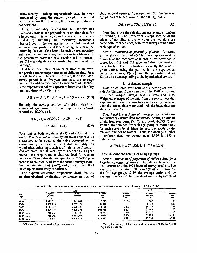
3. A &tailed example Data on children ever born and surviving are avail-

able for Thailand from a sample of the 1970 census and from two sample surveys held in 1974 and 1975. Weighted averages of the data from the two surveys that approximate those refemng to a point exactly five years after the census date were used. All the basic data are shown in table 65.

Steps 1 and 2: calculation of average parity and of average number of chilhen &adper woman. Average numbers of children ever born, P(i j ) , and dead, ACD(i,j), per woman are obtained for each age group of women and for each survey by dividing the recorded totals by the relevant number of women. Thus, the average number of children dead per woman aged 25-29 in 1970 is obtained as

Table 66 shows the results for all age groups.

Step 3: estimation of proportion of children dead for a hyptherical cohort of wemen. The interval between the 1970 census and the 1975 blended survey results is five years, so n in equations (D.3) and (D.4) is I . Thus, for the first age group, 15-19, the average parity and the average number of children dead for the hypothetical

TABLE 65. NUMBER OF WOMEN. CHILDREN EVER BORN AND CHILDREN DEAD. BY AGE GROUP. THAILAND. 1970 AND 1975

- 1970' - 1975

Aff N m k r Clulclhn ~ k i i N M b n C h k n C l u k n P v 4- m r h d d o/- ewr brn clrod (1) (3) 13) (4) (9 (6) (7L 15-19 ........ 1 883 232 245 069 15 223 13 054 1 662 188 20-24 ... . .. . . 1 359 859 1 367 179 99 316 10 037 8 839 600 25-29 ........ 1 141 937 2 795 340 74 526 7 812 16 787 1 329 30-34 . . . . . . . . 1 075 972 4 175 274 504 766 6 508 22 969 2 375 35-39 ........ 956315 4 93 1 749 732 342 6 244 29 557 3 515 40-44 . . . . . . . . 765 291 4 477 365 829 656 5 454 31 298 4 598 45-49 ........ 596 648 3 608 055 821 915 4 388 27 550 4 941

'Obtained rmm an expanded 2 per cent sample. qweighted average of the 1974 and 1975 rounds of the Survey of Population Change.

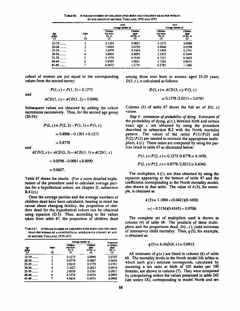
TABLE 66. AVERAGE NUMBER OF CHILDREN EVER BORN AND CHILDREN DEAD PER WOMAN. BY AGE GROUPOF MOTHER.THAILAND. 1970 AND 1975

I970 197s Avenlgemano/: A wmgr Man o/:

Childhn C h i h ChiIrfm Chilctrn A F Indrx em bDn dnd ~ r b o m &ad PV i flk 1) ACD(1.I) fli . 2) AC&i. 2)

(1) (2) (3) (4) (6)

cohort of women are put equal to the corresponding values from the second survey:

P(l , s ) = P( l ,2)= 0.1273 and

ACD(1, s ) = ACD(1,2)= 0.0090.

Subsequent values are obtained by adding the cohort increments successively. Thus, for the second age group (20-24):

= 0.8778 and

ACD(2, s)= ACD(2,2)-ACD(1, l)+ACD(l, s )

Table 67 shows the results. (For a more detailed explanation of the procedure used to calculate average parities for a hypothetical cohort, see chapter 11, subsection B.4 (c).)

Once the average parities and the average numbers of children dead have been calculated, bearing in mind the caveat about changing fertility, the proportion of children dead for the hypothetical cohort can be obtained using equation (D.5). Thus, according to the values taken from table 67, the proportion of children dead

TABLE 67. AVERAGE NUMBER OF CHILDREN EYER BORN AND CHII-DREN DEAD PER WOMAN OF A HYPOTHETICAL INTERSURVEY COHORT. BY AGE

OF MOTHER. THAILAND. 1970- 1975

among those ever born to women aged 25-29 years, D(3, s), is calculated as follows:

Column (5) of table 67 shows the full set of D(i , s ) values.

Step 4: estimation of probability of dying. Estimates of the probability of dying, q(x), between birth and certain exact age x are obtained by using the procedure described in subsection B.2 with the North mortality pattern. The values of the ratios P(l)lP(2) and P(2)/P(3) are needed to estimate the appropriate multipliers, k (i ). These ratios are computed by using the parities listed in table 67 as illustrated below:

The multipliers, k(i), are then obtained by using the equation appearing at the bottom of table 47 and the coefficients corresponding to the North mortality model, also shown in that table. The value of k(3). for example, is obtained as

The complete set of multipliers used is shown in column (4) of table 68. The products of these multipliers and the proportions dead, D(i, s), yield estimates of intersurvey child mortality. Thus, q(5). for example, is obtained as

All estimates of q(x) are listed in column (6) of table 68. The mortality levels in the North model life tables to which each q(x) estimate corresponds, calculated by assuming a sex ratio at birth of 105 males per 100 females, are shown in column (7). They were computed by interpolating within the values presented in table 242 (see annex IX), corresponding to model North and sex

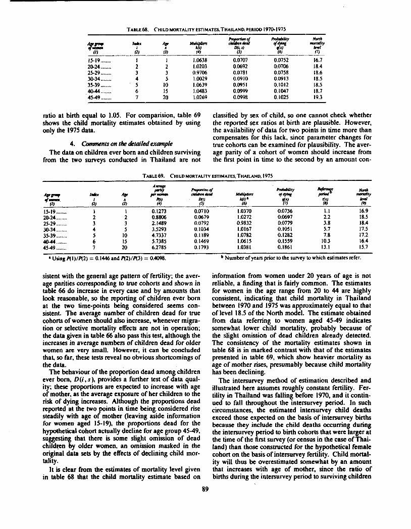
TABLE68. CHILD MORTALITY ESTIMATESTHAILAND. PERIOD 1970- 1975

ratio at birth equal to 1.05. For comparision, table 69 classified by sex of child, so one cannot check whether shows the child mortality estimates obtained by using the reported sex ratios at birth are plausible. However, only the 1975 data. the availability of data for two points in time more than

compensates for this lack, since parameter changes for 4. CmYnents on the &railed example true cohorts can be examined for plausibility. The aver-

The data on children ever born and children surviving age parity of a cohort of women should increase from from the two surveys conducted in Thailand are not the first point in time to the second by an amount con-

TABLE 69. CHILD MORTALITY ESTIMATES. THAILAND. 1975

Using F( I)lP(2) = 0.1446 and P(2)/P(3) = 0.4098. Number o f years prior to the survey to which estimates refer.

sistent with the general age pattern of fertility; the average parities corresponding to true cohorts and shown in table 66 do increase in every case and by amounts that look reasonable, so the reporting of children ever born at the two time-points being considered seems consistent. The average number of children dead for true cohorts of women should also increase, whenever migra- tion or selective mortality effects are not in operation; the data given in table 66 also pass this test, although the increases in average numbers of children dead for older women are very small. However, it can be concluded that, so far. these tests reveal no obvious shortcomings of the data.

The behaviour of the proportion dead among children ever born, D ( i , s), provides a further test of data quality; these proportions are expected to increase with age of mother, as the average exposure of her children to the risk of dying increases. Although the proportions dead reported at the two points in time being considered rise steadily with age of mother (leaving aside information for women aged 15-19), the proportions dead for the hypothetical cohort actually decline for age group 45-49, suggesting that there is some slight omission of dead childnn by older women, an omission masked in the original data sets by the effects of declining child mortality.

It is clear from the estimates of mortality level given in table 68 that the child mortality estimate based on

information from women under 20 years of age is not reliable, a finding that is fairly common. The estimates for women in the age range from 20 to 44 are highly consistent, indicating that child mortality in Thailand between 1970 and 1975 was approximately equal to that of level 18.5 of the North model. The estimate obtained from data refemng to women aged 45-49 indicates somewhat lower child mortality, probably because of the slight omission of dead children already detected. The consistency of the mortality estimates shown in table 68 is in marked contrast with that of the estimates presented in table 69, which show heavier mortality as age of mother rises, presumably because child mortality has been declining.

The intersurvey method of estimation described and illustrated here assumes roughly constant fertility. Fer- tility in Thailand was falling before 1970, and it contin- ued to fall throughout the intersurvey period. In such circumstances, the estimated intersurvey child deaths exceed those expected on the basis of intersurvey births because they include the child deaths occumng during the intersurvey period to birth cohorts that were larger at the time of the first survey (or census in the case of Thai- land) than those constructed for the hypothetical female cohort on the basis of intersurvey fertility. Child mortality will thus be overestimated somewhat by an amount that increases with age of mother, since the ratio of births during the intersurvey period to surviving children

at the beginning of the intersurvey period declines with As usual, it is helpful to have the data on children age of mother. Thus, it is surprising to find that the ever born and dead classified by sex. When this estimated mortality levels given in table 68 tend to classification is not available, sex differentials in child increase somewhat with age of mother in spite of the mortality can only be imputed by using mortality fact that the methodological bias just described would models. affect them in the opposite direction. Zlotnik and ~ i l l ' j estimated that the magnitude of this bias in the case of 3. Compuatio~l procedure Thailand is approximately -0.1 of a mortality level for The steps of the computational procedure are given the estimate derived from age group 25-29, and of about below. -0.2 of a mortality level for that derived from age step 1: o/awraFpufrypr T~ cal- group 30-34. The fact that such small biases a n coun- culate the average parity per P(i, j ) , let teracted by other, yet undetected. flaws in the data make CEB(~, j) be the number of children ever born to the average level, 18.5, an acceptable estimate of inter- women in age (duration) group at survey j, and let survey child mortality. FP(i, j) be the corresponding total number of women

E. ESTIMATION OF CHILD MORTALITY WHEN THE (ever-mamed women if data are classified by duration) FERTILITY EXPERIENCE OF TRUE COHORTS IS KNOWN age group i. Then, as Ihe average

number of children ever born per woman of age group i 1. Basis of methad and its rafio~le and survey j is calculated as

As explained in section A, if fertility has been changing in the recent past, the observed parity ratios used as P(i, j ) = CEB(i, j)/FP(i, j). (E.1) independent variables when estimating the multipliers, k (i), may not reflect adequately the true experience of Step 2: calculation ofproportion ofchi/hn dead reported cohorts in the population; and, hence, the resulting mul- ut time of second surwy. The values of this proportion, tipliers may not be suited for mortality estimation D(i, 2). are calculated only for the second survey or purposes. A method proposed to circumvent the prob- census. Thus, denoting the number of children dead to lems introduced by declining fertility consists of taking women of age group i from this survey by CD(i, 2). one into account the experience of true cohorts when has estimating the k(i) multipliers, instead of basing their estimates on ratios of parities referring only to one point D(i, 2)= CD(i, 2)/CEB(i, 2). in time. This method is described below in detail.

(E.2)

As in the methods presented before, two types of Step 3: calculation of multipliers. It is in this step that cohorts may be considered: those defined according to the use of cohort experience becomes relevant. The age; and those defined according to the duration of first values of multipliers k(i) are estimated by means of marriage or union. The estimation procedures used to equations fitted to model cases by means of least-squares analyze each of these types of data are very similar, so regression and whose independent variable is a ratio of only the case where data are classified by age is parities referring to a birth cohort of women at two described; the variations necessary to apply these pro- points in time. Therefore, if the surveys considered are ccdures to data classified by duration of first mamage five years apart, these parity ratios have the form are pointed out as the need arises. P(i - I , I)lP(i ,2); while if the surveys are 10 years

2. h a required apart, the corresponding ratios would be P(i -2, l)/P(i, 2). The form of the equation to esti-

The following data are required for this method: mate the k(i) multipliers, the values of the fitted (a) The number of children ever born classified by coefficients and the form of the corresponding parity

five-~ear age (or duration) group of mother for two sur- ratios are presented in tables 70-73. Tables 70 and 71 veys five or 10 years apart; are to be used when the data are classified by age,

(b) The number of children dead (or surviving) whereas tables 72 and 73 are needed when the data are classified by five-year age (or duration) group of mother classified by duration of first marriage. The first table of for the most recent survey being considered; each set (tables 70 and 72) is to be used when the inter-

(c) The total number of women (or of ever-mamed Survey interval is five years, whereas the second table of women) classified by five-year age (or duration) groups each set (tables 71 and 73) is needed when the interval is for each one of the surveys being considered. 10 years. After selecting the appropriate table for the

It is not necessary to have data on the number of chil- case at hand, the calculafion of the k(i) multipliers is dead for both of the surveys being considered. If straigh'orvud* as is in the exam~'es.

these data are available (children dead for both surveys), S?P 4: estimation ? f m I i ! Y ofdyng- The estimated it is strongly recommended that the method described values of q(x), the probability of dying between birth above in.section D be used to estimate intersurvey child and exact age x* are as the products the mortality, in spite of the fact that it does not make any obsewed proportions. dead, ~ ( i , 2), and the multipliers, explicit allowance for the effects of changing fertility. k (i ), computed in step 3.

Step 5: estimation of reference period. The use of the I3 lbid. experience of true cohorts to estimate the multipliers,

90

TABLE 70. COEFFICIENTS FOR ESTIMATION OF THE MULTICLIERS, k(i). FROM THE EXPERIENCE Of TRUE ConOI'lS WHEN DATA ARE CLASSIFIED BY AOE OF MOTH& AND THE IW1EIUURVEY INTERVAL IS FIVE YEARS

Nmh . . . . . . . 20-24 25-29 3@34 35-39

South ....... 20-24 25-29 30-34 35-39

East . . . . . . . . . . 20-24 25-29 30-34 35-39

West . . . .. . . .. 20-24 25-29 30-34 35-39

Estimation equations: k ( i ) = a ( i ) + b ( i ) P(i - 1, l ) /P ( i , 2 ) q (x )= k ( i ) D ( i . 2 )

T m L E 71. CoePPrc lem ~o l l esnnunolr OF THE ~ u ~ n n r e W k (I ), m a me exreulwc~ OF TRue cono~fs WH@N DATA ARE CLASSIFIED BY AOE OF MOTHER AND THE INTERSURVEY IlHlPRVAL IS 10 YEARS

North ....... 25-29 30-34 35-39

Edimation equations: k( i )=a ( i )+b ( i ) P( i -2. l ) /P ( i , 2 ) q (x )= k ( i ) D ( i . 2 )

k(i), makes allowance for changes in fertility, but it docs nothing with respect to changes in mortality. Therefore, if there is evidence suggesting a mortality decline in the recent past, it is important to ascertain to which time period the q(x) estimates obtained in step 4 really refer. The estimation of the reference period, r(x), the number of years before the second survey to which the comsponding q(x ) estimate refers, is camed out by means of equations whose coefficients were estimated by using least-squares regression applied to data generated by model schedules. The estimated values of thcse coefficients a n given in tables 74-77. The order of these tables parallels that used in present- ing the tables needed calculate the k(i) multipliers. The first two tables are qscd when data are classified by age and the second two when data are classified by mar-

riage duration. Within each set, the first table is used if the intersurvey period is five years and the second if it is 10 years. The use of these tables is illustrated in the next exampIes.

4. &lcltlcltlrd exaqdes This section presents two examples: that used in the

previous section referring to Thailand and illustrating the estimation procedure applied to a five-year intersurvey interval; and the case of Brazil, where data on children ever born and children surviving have been collected by several of its decennial censuses.

(a) WIM 1970-1975

The basic data available for Thailand for the years

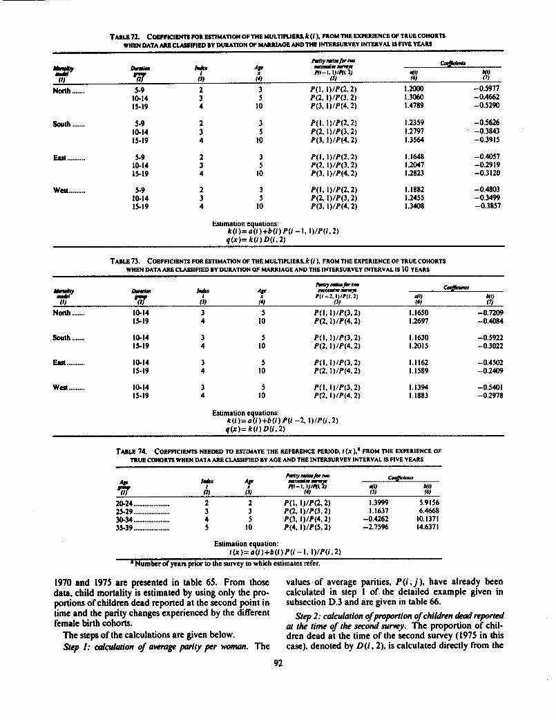
TABLE 72. C~~PPICIENTS FOR ISTIMATION OF THE MULTIPLIERS, k (i ), FROM THE EXPERIENCE OF TRUE COHORTS WHEN DATA AM CUP(IflED BY WMTtON OF MARRIAOE AND THE INTERSURVEY INTERVAL IS f lVE YEARS

W l y Wafi M

%2P h b r I h -*wryr CorjidnmJ

57 I A!' dl) W mi- I, l)/Rl, 1) (1)' (3) (4) fJ) (6) f 7)

Nodl ....... 5-9 2 3 P(1. I)lP(2.2) 1.2000 10-14 3

-0.5977 5 P(2. I)/P(3,2) 1.3060

15-19 4 -0.4662

10 P(3. I )lP(4.2) 1.4789 -0.5290

....... South 5-9 2 3 P(l. I)lP(2.2) 1.2359 -0.5626 10-14 3 5 P(2. IllP(3.2) I .2797 -0.3843 15-19 4 10 P(3, I)lP(4.2) 1.3564 -0.3915

Estimation equations: k(i)=a(i)+b(i)P(i -1, l)/P(i,2) q(x)= k(i) D(i, 2)

T ~ 8 L e 7 3 . COEFFICIENTS FOR ESTIMATION OF M E MULTIPLIERS k(i ), FROM THE EXPERIENCE OF TRUE COHORTS WHEN DATA ARE CLASSIFIED BY DURATION OF MARRIAGE AND THE INTERSURVEY INTERVAL IS 10 YEARS

LL.*bn I h "&"a&- co* %ZY 7 I A!' p t i -2. I)IP(I. 2) dl) MU (1) (3) (4) fJ) (6) f 7)

North ....... 10-14 3 5 P(l, I)lP(3,2) 1.1650 -0.7209 15-19 4 10 P(? 1)lP(4.2) 1.2697 -0.4084

South ....... 10-14 3 5 P(l , 1)/P(3.2) 1.1630 -0.5922 15-19 4 10 P(2, 1 )/P(4.2) 1.2015 -0.3022

Estimation equations: k(i)= a(i)+b(i)P(i -2, I)/P(i, 2) a(x)= k(i) D(i. 2)

TABLE 74. COEFFICIENTS NEEDED TO ESTIMATE THE REFERENCE PERIOD. I (X ): FROM THE EXPERIENCE OF TRUE COHORTS WHEN DATA me CLASSIFIED BY AGE AND THE INTERSURVEY INTERVAL IS FIVE YEARS

Estimation equation: ~ (x)=a( i )+b( i )P( i -I, l)/P(i, 2)

Number of yean prior to the survey lo which estimates rrfer.

1970 and 1975 are presented in table 65. From those values of average parities, P ( i , j), have already been data, child mortality is estimated by using only the pro- calculated in step 1 of. the detailed example given in portions of children dead reported at the second point in subsection D.3 and are given in table 66. time and the parity changes experienced by the different step 2: ofpmprtiOn ofchildren reprtd female birth cohorts. ar the time of the second surwy. The proportion of chil-

The steps of the calculations are given below. dren dead at the time of the second survey (1975 in this Step I: calculation of awmgc parity per wman. The case), denoted by D( i ,2), is calculated directly from the

TABU 75. COEPflClEN?S NEEDED lU ESTIMATE THE REFEREWE PERIOD, I(x),' FROM THE EXPERIENCE OF TRUECOHORTS WHEN DATA ARECLMSlflED BY AOE ANDTHE INTERSURVEY INTERVAL IS 10 YeAflS

Estimation equation: t(x)=a(i)+b(i) P(i -2. I)/P(i. 2)

'See u b k 74. footnote a.

TABLE 76. COEFFlCleMs NEEDED l 0 WIIMATE THE REFERENCE PERIOD, I (X ),' FROM THE EXPERIENCE OF TRUE COHORTS WHEN DATA M E CLASSIFIED BY MARRlAOE DURATION ANDTHE INTERSURVEY INTERVAL IS fIVE YEARS

Estimation quation: t(x)=a(i)+b(i) P(i -I, l)/P(i,2)

See table 74. footnote a.

TABLE 77. CO~PP~CIENTS NEEDED 'TV WlIMAl'E THE R E W N C E PERIOD, t (x): FROM THE EXPERIENCE OF TRUE COHORTS WHEN DATA ARE CLASSIFIED BY MARRIAOE DURATION ANDTHE INTERSURVEY INTERVAL IS I0 \,EARS

Estimation equation: r(x)=a(i)+b(i) P(i -2, I)/P(i, 2)

'See u b k 74. footnote a.

data given in table 65 by dividing the number of chil- since the intersurvey period is five years. The values of dren dead by those ever born for each age group of these ratios are shown in column (5) of table 78. For mother. For example, D(4,2) is calculated as follows: i = 4, the ratio is

All values of D(i, 2) are shown in table 78. where the values of P(i -I, 1) and P(i, 2) are obtained Step 3: calculation 4 dtipliem. The independent from table 66-

variables necessary to estimate the multipliers, k(i), are Once the necessary parity ratios are computed, the the.ratios of the observed average parities corresponding values of k ( i ) are estimated by using the coefficients to true cohorts at the two points in time being con- presented in table 70. As in the example given in sub- sidend. These ratios have the form P(i - I, I)/P(i, 2), section D.3, the mortality pattern selected is North. The

TABue78. ESTIMATION OF CHILD MORTALITY PROM 1975 DATATAKINO INTO ACCOUNT THE FERTILITY EX?ERlENCE OF COHORT~TWLAND

resulting values of k(i) are shown in table 78; k(4) is second survey. So it can be said that q(2) roughly calculated in detail below: represents the child mortality prevalent in 1973. since

the second data set being considered is supposed to k (4)= 1.3408 +(-0.52 10)(0.6936) = 0.9749. represent 1975 experience. The complete set of t(x)

values is listed in table 78.

Step 4: calculation of probability of dying. Estimates of the probability of dying, q(x), are obtained as the products of the proportion of children dead, D(i, 2), and the k(i) multipliers. Note that this time no estimate of q(l) is possible; consequently, there is no multiplier for D(1.2). The resulting values of q(x) are shown in column (7) of table 78.

Step 5: calculation of reference period. Using the coefficients presented in table 74 and the parity ratios used in calculating k(i), the values of the reference period. t(x), are obtained by substituting them in the estimation equation shown at the bottom of table 74. For example,

This value means that the estimate of q(2) obtained in step 4 refers to approximately 2.3 years before the

Column (9) of table 78 shows the levels of mortality in the North family of Coale-Demeny life tables consistent with the estimated q(x) values. Once more, these levels suggest that child mortality has been declining. Their values are quite consistent with those shown in table 69, where child mortality estimates were obtained solely from the 1975 data. If anything. the new values suggest that the decline in mortality was more rapid.

(b) Brazil, 1960-1 970 The data on children ever born and surviving col-

lected for the whole of Brazil during the 1960 and 1970 censuses (both of which have exactly the same reference date, 1 September) are given in table 79. This wealth of data permits the application of most of the methods described in this chapter. Since the detailed application of these methods has already been described in the other examples presented so far, it is not repeated here, but results obtained by using each of them are shown.

TABLE 79. DATAON CHILDREN EVER BORN AND SURVIVING. BRAZIL. 1960 AND 1970 ( n o ~ n d r )

Before proceeding to apply these methods, it must be pointed out that the question used in the 1960 census to obtain information on children ever born was not phrased properly; consequently, the data collected exhibit a definite bias. Specifically, the question asked of women of reproductive age was: "How many children have you ever had?", instead of "How many children, who have been born alive, have you ever had?" It is therefore likely that the 1960 information on children ever born includes both those born alive and those born dead. So, before the 1960 data are used to estimate child mortality, the number of children ever born have to be corrected for the inclusion of stillbirths. The correction made consists in multiplying the reported numbers of children ever born by 0.97, on the assumption that the incidence of stillbirths among all births is 0.03. In studies of similar data collected during the 1950 census of Brazil, the proportion of stillbirths used for the purpose of correction was 0.05.'~ This estimate was based on the proportion of stillbirths yielded by the 1940

14 Giorgio Mortara, "A fecundidade da mulher e a sobrevivencia dos filhos no Brasil. se undo o Censo de 1950". Contribuc6esparo o Es- ,I& d. &no @ da Brasdl (Rio de Janeiro, Fundacao lnrituto Brasileiro de 6eoRrafia e Estatistica. 1970): and J. A. M. Calvalho. "Regional trends of fertility and mortality in Brazil", Popula~ion Stud- ies, vol. XXVIII, No. 3 (November 1974), pp. 401-421.

census, during which a definite distinction was made between live births and stillbirths. According to this census, about 7 per cent of all births were stillbirths, but the estimate of 5 per cent was accepted on the grounds that women were not as likely to report all their stillbirths when only a question on children ever born was posed as when two questions, one about live births and another about stillbirths, were asked.

More information about the incidence of stillbirths among all births to the Brazilian population is now available. Two separate questions referring to these events were asked by the 1970 census and by several country-wide sample surveys carried out during the 1970s. All these data reveal that the proportion of reported stillbirths among all births has declined to roughly 0.05 (0.045 may be a more accurate figure): and therefore, a 5 per cent correction for the 1960 data seems too high, especially because of the known tendency among women to underreport the number of children they have ever had. As a compromise, a 3 per cent correction was accepted. The corrected numbers of children ever born by age group of mother for 1960 are shown in column (4) of table 79.

Table 80 shows the results of the steps needed to estimate child mortality from the information gathered in

TABLE 80. CHILD MORTALITY ESTIMATION USING MULTIPLIERS BASEDON THE WEST MORTALITY PAlTERN, BRAZIL. 1960

Ax Tk hb&Uty - war An lrdrx

I 9= "r(T a i d Multip@ ddyl~ WY

b.T mi) Mi) 0) (2) (3) (4) (!!-- (6) 7;) (8) A --

%'

' Adjus ted t o exclude stillbirths. Number of years prior t o the s u r v e y t o which e s t i m a t e s refer . Based on P(I)lP(2)= 0.1 138 and P(2)lP(3)= 0.4335.

TABLE 81. CHILD MORTALITY ESTIMATION USING MULTIPLIERS BASED ON THE WEST MORTALITY PATTERN. BRAZIL, 1970

A m q * pUy = Wbt

A l Indrx f P"- w t i p p s o/m P f

I;, ryi) Wi) 4 0 76) (1) (3) (4) (-0 16) (8)

Y? (91

15-19 .................... I 1 0.1 187 0.1 159 1.1168 0.1294 1 .O 13.0 20-24 .................... 2 2 0.9705 0.1265 1.0850 0.1373 2.1 14.3 25-29 .................... 3 3 2.4274 0.1396 1.0258 0.1432 3.8 14.6 30-34 .................... 4 5 3.7764 0.1550 1.0298 0.1596 5.9 14.5

'Based on P(I)lP(2)= 0.1223 and P(2)IP(3)= 0.3998 See t a b l e 80, f o o t n o t e c.

1960 (see subsection B.2). Note that the levels of mortality implied by the q(x) estimates are fairly similar, except for that associated with q(l), which is clearly out of line with the rest, probably because child mortality is not independent of mother's age (see subsection A.l).

Note that the raw data (table 79) provide the number of children surviving rather than the number dead. The latter, of course, are obtained by subtraction.

Table 81 shows the estimates of childhood mortality obtained solely from the 1970 information (see subsection 8.2). Once more, the estimate of q(1) is not consistent with the others. In general, the level of child mortality seems to have improved between 1960 and 1970.

It is worth remarking that when child mortality is estimated from a single data set, the estimated values of

q(l), q(2). q(3) and q(5) refer approximately to one, two, four and six years before the census being considered. Reference dates for the usual child mortality estimates always display this pattern.

Tables 82 and 83 illustrate the steps necessary to obtain intercensal estimates of child mortality (see section D). The average number of children dead is obtained in this case by subtracting the number of children surviving from the total number of children ever born and dividing the result by the number of women in the relevant age group. Thus, for example,

Final results are shown in table 83. Note that the

TABLE 82. CHILD MORTALITY ESTIMATION FOR THE INTERCENSAL PERIOD 1960-1970. WITH 1960 DATA ON CHILDREN EVER BORN CORRECTED FOR INCLUSION OF STILLBIRTHS. BRAZIL

15-19 .................... I 0.1217 0.1187 0.0148 0.0138 0.0 138 20-24 .................... 2 1.0686 0.9705 0.1488 0.1228 0.1228 25-29 .................... 3 2.4650 2.4274 0.3828 0.3388 0.3378 30-34 .................... 4 3.6865 3.7764 0.6464 0.5853 0.5593 35-39 .................... 5 4.7610 4.8009 0.944 1 0.8222 0.7771

'Adjus ted t o exclude stillbirths.

TABLE^^. INTERCENSAL ESTIMATES OF CHILD MORTALITY. BRAZIL. 1960-1970

-

15-19 .................... I I 0.1 187 0.1 163 1.1172 0.1299 12.9 20-24 .................... 2 2 0.9705 0.1265 1.0849 0.1372 14.4 25-29 .................... 3 3 2.4244 0.1393 1.0256 0.1429 14.7 30-34 .................... 4 5 3.6783 0.1521 1.0296 0.1566 14.6 35-39 .................... 5 10 4.7927 0.1621 1.0460 0.1696 14.6

'Based on P(I)IP(2)= 0.1223 and P(2)lP(3)= 0.4003.

TluLe 84. CHILD MORTl*lsn WnMATlON TNClNO INTO ~cc0UNl'mE EJWEWENCE OF nve COHORT& BRAZIL 1970

mw& M Y '-5' IIC* I d a

1 9' mi-z 1 IN& 2) 81 0) (4 T

IS) #$? (6)

% (7)

* (8)

25-29 .................... 3 3 0.0501 1.0138 0.1415 4.0 14.7 3Q-34 .................... 4 5 - 0.2830 1.0166 0. I576 6.2 14.6 35-39 .................... 5 10 0.5 134 1.0352 0.1773 8.7 14.3

'Number of yean prior to the curvey to which estimates refer.

mortality levels prevalent during the intercensal period almost the same mortality levels are obtained (see table almost coincide with those obtained solely from the 1970 84). Such consistency is reassuring. It permits one to data; and, excluding q(l), they are fairly consistent. conclude that the average West mortality level prevalent

Lastly, when estimates for 1970 are obtained by tak- during the period 1960-1970, as measured by child mor- ing into account the fertility experience of true cohorts, tality, was approximately 14.5.

ADLMTIONAL REFERENCES

Bnrr, William. Cuatro lecciones de William Bnss. Slntiago de Chile, Tfusell. T. J. and K. Hill. Fertility and mortality estimated from the Cenm Lationamericmo de Demognfla, 1977. (CELADE rries D, Panama Retrospective Demographic Survey. 1976. Popuhrion 91) std&s(London) 343) : 551-563, November 1980.

Bnrr, William end orhers. The demognphy of tmpicrl Africa. Prince- ton, New Jersey. Princeton Univeaity Press, 1968. United Nations. Department of Economic and Social Allain. Manual

Hill. K. and J. Trussell. Further developmenls in indirect mortality IV. Methods of estimating basii demographic measures from estimation. Fbpu&fion surdks(London) 31(2) : 313-333, July 1977. incomplete data. (Population studies. 42) Sales No. E.67.Xl11.2.

-ter of on children ever born and children surviving · dead among the children ever borne by a...

Documents