Tensor networks and deep learning

I. Oseledets, A. CichockiSkoltech, Moscow

26 July 2017

What is a tensor

Tensor is 𝑑-dimensional array:

𝐴(𝑖1, … , 𝑖𝑑)

Why tensors

Many objects in machine learning can be treated as tensors:▶ Data cubes (RGB images, videos, different

shapes/orientations)▶ Any multivariate function over tensor-product domain can be

treated as a tensor▶ Weight matrices can be treated as tensors, both in

Conv-layers and fully-connected layersUsing tensor decompositions we can compress data!

Compression of neural networks

Compression of conv-layers

Lebedev V. et al. Speeding-up convolutional neural networks usingfine-tuned cp-decomposition arXiv:1412.6553.

In a generalized convolution the kernel tensor is 4D(𝑑 × 𝑑 × 𝑆 × 𝑇 ) (spatial, input, output).

If we construct rank-𝑅 CP-decomposition, that amounts to havingtwo layers of smaller total complexity, than the full layer.

The idea: use TensorLab (best MATLAB code forCP-decomposition) to initialize these two layers, and then fine-tune

Result: 8.5x speedup with 1% accuracy drop.

Compression of FC-layer

Novikov, Alexander, et al. ”Tensorizing neural networks.” Advancesin Neural Information Processing Systems. 2015.

Use tensor-structured representation, up to 1000x compression of afully-connected layer.

Tensor RNN

Recent example: Yang, Yinchong, Denis Krompass, and VolkerTresp. ”Tensor-Train Recurrent Neural Networks for Video

Classification.” arXiv:1707.01786

3000 parameters in TT-LSTM vs 71,884,800 in LSTM

Accuracy is better (due to additional regularization)

Idea of tensorization

We can find tensors even in simple object!

Quantized Tensor Train format:

Take a function 𝑓(𝑥) = sin𝑥, discretize in on 2 × … × 2 grid

Reshape into a 𝑑-dimensional tensor.

Gives log𝑁 complexity to represent classes of functions.

Connection between TN and Deep Learning

Recent work by Cohen, Shahua et. al.

Shows that tensor decompositions are neural networks withproduct pooling

Tensor notation

Simplest tensor network

The simplest tensor network is matrix factorization:

𝐴 = 𝑈𝑉 ⊤.

Why matrix factorization is great

𝐴 ≈ 𝑈𝑉 ⊤

▶ Best factorization by SVD▶ Riemmanian manifold structure▶ Nice convex relaxation (nuclear norm)▶ Cross approximation / skeleton decomposition

Cross approximation / skeleton decomposition

One of underestimated matrix facts:

If a matrix is rank 𝑟, it can be represented as

𝐴 = 𝐶𝐴−1𝑅,

where 𝐶 are some 𝑟 columns of 𝐴, 𝑅 are some rows of 𝐴, 𝐴 is asubmatrix on the intersection.

Maximum-volume principle

Goreinov, Tyrtyshnikov, 2001 have shown:

If 𝐴 has maximal volume, then

‖𝐴 − 𝐴𝑠𝑘𝑒𝑙‖𝐶 ≤ (𝑟 + 1)𝜎𝑟+1.

Way to compare submatrices!

Riemannian frameworkLow-rank matrices form a manifold

Standard: 𝐹(𝑋) = 𝐹(𝑈𝑉 ⊤) → min

Riemmanian:

Riemannian word embedding

Example: Riemannian Optimization for Skip-Gram NegativeSampling A Fonarev, O Hrinchuk, G Gusev, P Serdyukov

arXiv:1704.08059, ACL 2017.

We treated SGNS as implicit matrix factorization and solved inusing Riemannian optimization.

Tensor factorization

Tensor factorization: we want numerical tools of thesame quality

Classical attempt

Matrix case:

𝐴(𝑖, 𝑗) =𝑟

∑𝛼=1

𝑈(𝑖, 𝛼)𝑉 (𝑗, 𝛼).

CP-decomposition:

𝐴(𝑖, 𝑗, 𝑘) =𝑟

∑𝛼=1

𝑈(𝑖, 𝛼)𝑉 (𝑗, 𝛼)𝑊(𝑘, 𝛼)

Tucker decomposition:

𝐴(𝑖, 𝑗, 𝑘) =𝑟

∑𝛼,𝛽,𝛾=1

𝐺(𝛼, 𝛽, 𝛾)𝑈(𝑖, 𝛼)𝑉 (𝑗, 𝛽)𝑊(𝑘, 𝛾)

CP-decomposition has bad properties!

▶ Best rank-𝑟 approximation may not exist▶ Algorithms may converge very slowly (swamp behaviour)▶ No finite-step completion procedure.

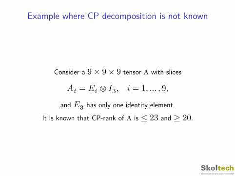
Example where CP decomposition is not known

Consider a 9 × 9 × 9 tensor A with slices

𝐴𝑖 = 𝐸𝑖 ⊗ 𝐼3, 𝑖 = 1, … , 9,and 𝐸3 has only one identity element.

It is known that CP-rank of A is ≤ 23 and ≥ 20.

Example where CP decomposition does not exist

Consider

𝑇 = 𝑎 ⊗ 𝑏 ⊗ … ⊗ 𝑏 + … + 𝑏 ⊗ … ⊗ 𝑎.

Then,

𝑃(𝑡) = ⊗𝑑𝑘=1(𝑏+𝑡𝑎), 𝑃 ′(0) = 𝑇 = 𝑃(ℎ) − 𝑃(0)

ℎ +𝒪(ℎ).

Can be approximated with rank-2 with any accuracy, but no exactdecomposition of rank less than 𝑑 exist!

Our idea

Our idea was to build tensor decompositions usingwell-established matrix tools.

Reshaping tensor into matrix

Let reshape an 𝑛 × 𝑛 × … × 𝑛 tensor into a 𝑛𝑑/2 × 𝑛𝑑/2

matrix 𝐴:

𝔸(ℐ, 𝒥) = 𝐴(𝑖1 … 𝑖𝑘; 𝑖𝑘+1 … 𝑖𝑑)and compute low-rank factorization of 𝔸:

𝔸(ℐ, 𝒥) ≈𝑟

∑𝛼=1

𝑈(ℐ, 𝛼)𝑉 (𝒥, 𝛼).

Recursion

If we do it recursively, we get 𝑟log 𝑑 complexity

If we do it smart, we get 𝑑𝑛𝑟3 complexity:▶ Tree-Tucker format (Oseledets, Tyrtyshnikov, 2009)▶ H-Tucker format (Hackbusch, Kuhn, Grasedyck, 2011)▶ Simple but powerful version: Tensor-train format (Oseledets,

2009)

Canonical format and shallow network

N. Cohen, A. Shashua et. al provided an interpretation of thecanonical format as a shallow neural network with a product

pooling

𝐴(𝑖1, … , 𝑖𝑑) ≈𝑟

∑𝛼=1

𝑈1(𝑖1, 𝛼)𝑈2(𝑖2, 𝛼) … 𝑈𝑑(𝑖𝑑, 𝛼).

H-Tucker as a deep neural network with productpooling

Tensor-train

TT-decomposition is defined as

𝐴(𝑖1, … , 𝑖𝑑) = 𝐺1(𝑖1) … 𝐺𝑑(𝑖𝑑),𝐺𝑘(𝑖𝑘) is 𝑟𝑘−1 × 𝑟𝑘, 𝑟0 = 𝑟𝑑.

Known for a long time as matrix product state in solid statephysics.

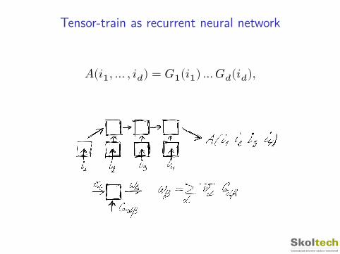
Tensor-train as recurrent neural network

𝐴(𝑖1, … , 𝑖𝑑) = 𝐺1(𝑖1) … 𝐺𝑑(𝑖𝑑),

Properties of the TT-format

▶ TT-ranks are ranks of matrix unfoldings▶ We can do basic linear algebra▶ We can do rounding▶ We can recover a low-rank tensor from 𝒪(𝑑𝑛𝑟2) elements▶ Good for rank-constrained optimization▶ There are classes of problems where 𝑟𝑘 ∼ log𝑠 𝜀−1

▶ We have MATLAB, Python and Tensorflow toolboxes!

TT-ranks are matrix ranks

Define unfoldings:𝐴𝑘 = 𝐴(𝑖1 … 𝑖𝑘; 𝑖𝑘+1 … 𝑖𝑑), 𝑛𝑘 × 𝑛𝑑−𝑘 matrix

TT-ranks are matrix ranks

Define unfoldings:𝐴𝑘 = 𝐴(𝑖1 … 𝑖𝑘; 𝑖𝑘+1 … 𝑖𝑑), 𝑛𝑘 × 𝑛𝑑−𝑘 matrix Theorem:

there exists a TT-decomposition with TT-ranks

𝑟𝑘 = rank 𝐴𝑘

TT-ranks are matrix ranks

The proof is constructive and gives the TT-SVD algorithm!

TT-ranks are matrix ranks

No exact ranks in practice – stability estimate!

TT-ranks are matrix ranks

Physical meaning of ranks of unfoldings is entanglement: we splitthe system into two halves, and if rank is 1, they are independent.

Approximation theorem

If 𝐴𝑘 = 𝑅𝑘 + 𝐸𝑘, ||𝐸𝑘|| = 𝜀𝑘

||A − TT||𝐹 ≤√√√⎷

𝑑−1∑𝑘=1

𝜀2𝑘.

TT-SVD

Suppose, we want to approximate:𝐴(𝑖1, … , 𝑖𝑑) ≈ 𝐺1(𝑖1)𝐺2(𝑖2)𝐺3(𝑖3)𝐺4(𝑖4)

1. 𝐴1 is an 𝑛1 × (𝑛2𝑛3𝑛4) reshape of A.2. 𝑈1, 𝑆1, 𝑉1 = SVD(𝐴1), 𝑈1 is 𝑛1 × 𝑟1 — first core3. 𝐴2 = 𝑆1𝑉 ∗

1 , 𝐴2 is 𝑟1 × (𝑛2𝑛3𝑛4).Reshape it into a (𝑟1𝑛2) × (𝑛3𝑛4) matrix

4. Compute its SVD:𝑈2, 𝑆2, 𝑉2 = SVD(𝐴2),𝑈2 is (𝑟1𝑛2) × 𝑟2 — second core, 𝑉2 is 𝑟2 × (𝑛3𝑛4)

5. 𝐴3 = 𝑆2𝑉 ∗2 ,

6. Compute its SVD:𝑈3𝑆3𝑉3 = SVD(𝐴3), 𝑈3 is (𝑟2𝑛3) × 𝑟3, 𝑉3 is𝑟3 × 𝑛4

Fast and trivial linear algebra

Addition, Hadamard product, scalar product, convolutionAll scale linear in 𝑑

Fast and trivial linear algebra

𝐶(𝑖1, … , 𝑖𝑑) = 𝐴(𝑖1, … , 𝑖𝑑)𝐵(𝑖1, … , 𝑖𝑑)

𝐶𝑘(𝑖𝑘) = 𝐴𝑘(𝑖𝑘) ⊗ 𝐵𝑘(𝑖𝑘),ranks are multiplied

Tensor rounding

A is in the TT-format with suboptimal ranks.How to reapproximate?

Tensor rounding

𝜀-rounding can be done in 𝒪(𝑑𝑛𝑟3) operations

Cross approximation

Recall the cross approximation

Rank-𝑟 matrix can be recovered from 𝑟 columns and 𝑟 rows

TT-cross approximation

Tensor with TT-ranks 𝑟𝑘 ≤ 𝑟 can be recovered from 𝒪(𝑑𝑛𝑟2)elements.

There are effective algorithms for computing those points in activelearning fashion.

They are based on the computation of maximum-volumesubmatrices.

Making everything a tensor: the QTT

Let 𝑓(𝑥) be a univariate function (say, 𝑓(𝑥) = sin 𝑥).

Let 𝑣 be a vector of values on a uniform grid with 2𝑑 points.

Transform 𝑣 into a 2 × 2 × … × 2 𝑑-dimensional tensor.

Compute TT-decomposition of it!

And this is the QTT-format

Making everything a tensor: the QTT

If 𝑓(𝑥) is such that

𝑓(𝑥 + 𝑦) =𝑟

∑𝛼=1

𝑢𝛼(𝑥)𝑣𝛼(𝑦),

then QTT-ranks are bounded by 𝑟Corollary:

▶ 𝑓(𝑥) = exp(𝜆𝑥)▶ 𝑓(𝑥) = sin(𝛼𝑥 + 𝛽)▶ 𝑓(𝑥) is a polynomial▶ 𝑓(𝑥) is a rational function

Optimization with low-rank constraints

Tensors can be given implicitly as a solution of a certainoptimization

𝐹(𝑋) → min, 𝑟𝑘 ≤ 𝑟.The set of low-rank tensors is non-convex, but has efficient

Riemannian structure and many fabulous unstudied geometricalproperties.

Desingularization

Desingularization of low-rank matrix manifolds(V. Khrulkov, I. Oseledets).

The set of matrices of rank smaller than 𝑟 is not a manifold (anymatrix of smaller rank is a singular point).

Desingularization of matrix varieties

Solution: consider pairs (𝐴, 𝑌 ) such that

𝐴𝑌 = 0, 𝑌 ⊤𝑌 = 𝐼, 𝑌 ∈ ℝ𝑚×(𝑛−𝑟).. Theorem. Pairs (𝐴, 𝑌 ) form a smooth manifold.

We can use pain-free second-order methods to optimize withlow-rank constraints.

Software

▶ http://github.com/oseledets/TT-Toolbox – MATLAB▶ http://github.com/oseledets/ttpy – Python▶ https://github.com/Bihaqo/t3f – Tensor Train in Tensorflow

(Alexander Novikov)

Application of tensors

▶ High-dimensional, smooth functions▶ Computational chemistry (electronic and molecular

computations, spin systems)▶ Parametric PDEs, high-dimensional uncertainty quantification▶ Scale-separated multiscale problems▶ Recommender systems▶ Compression of convolutional layers in deep neural networks▶ TensorNet (Novikov et. al) – very compact dense layers

Type of problems we can solve

▶ Active tensor learning by the cross method▶ Solution of high-dimensional linear systems: 𝐴(𝑋) = 𝐹▶ Solution of high-dimensional eigenvalue problems

𝐴(𝑋) = 𝜆𝑋▶ Solution of high-dimensional time-dependent problems

𝑑𝐴𝑑𝑡 = 𝐹(𝐴) (very efficient integrator).

Software

We have implemented tensor-train functionality in Tensorflow.

t3f

A library for working with Tensor Train on TensorFlow.

https://github.com/Bihaqo/t3f

▶ GPU support;▶ Easy to combine with neural networks;▶ Riemannian optimization support

Exponential machines

A. Novikov, M. Trofimov, I. Oseledets, Exponential Machines

Idea: use as features 𝑥1, 𝑥1𝑥2, …There are 2𝑑 coefficients, thus we can put low-rank constraint,

and the model is

𝑓(𝑥1, … , 𝑥𝑑) ≈ 𝑓1(𝑥1, 𝑖1) … 𝑓𝑑(𝑥𝑑, 𝑖𝑑)𝑊(𝑖1, … , 𝑖𝑑),and then we put low-rank constraint on 𝑊 .

Riemannian gradient modelling.

Model-based tensor reinforcement learning

Alex Gorodetsky, PhD dissertation, MIT (2017): tensor-train forreinforcement learning

Key components:▶ “Physical” state space (like 𝑥, 𝑦, 𝑧, 𝑣𝑥, 𝑣𝑦, 𝑣𝑧)▶ Model: 𝑑𝑥

𝑑𝑡 = 𝑓(𝑥,𝑢) + 𝛿 𝑑𝑊𝑑𝑡

As a result, Hamilton-Jacobi-Bellman equation for the optimalpolicy is solved using the cross method (note fundamental

differences to DNN-based Q-learning!)

Comments and open problems

▶ Tensor decompositions are good for regression of smoothfunctions (neural networks are not!)

▶ An important question: why deep learning works so well forclassification (the number of data points is much smaller,than the number of parameters)

▶ Can we combine the best of those approaches?

Some insights

▶ Tensor networks and convolutional aritmetic circuits are thesame!

▶ Network architecture reflects “correlations” betweensubsystems.

▶ Main question: can we (and need we?) use matrixfactorizations to get better algorithms for feed-forwardnetworks?

Megagrant

2017-2019: Megagrant under the guidance of Prof. Cichocki@Skoltech (deeptensor.github.io), “Deep leaning and tensor

networks”.▶ Victor Lempitsky (deep learning and computer vision)▶ Dmitry Vetrov (deep learning and Bayesian methods)▶ Ivan Oseledets (tensors)

Two monographs in Foundations and Trends in Machine Learningwith basic introduction to the field.