tensile failure criteria for fiber composite materials · 2013-08-31 · tensile failure criteria...

~~ --

NASA CONTRACT-O_.&.zJj

LOAN COPY: RETURPI v‘ ..rL. <DOUL) ‘,

WRTLAND AFB, N. hi. :I

TENSILE FAILURE CRITERIA FOR FIBER COMPOSITE MATERIALS

by B. Walter Rosen und Carl H. Zweben

Prepared by

MATERIALS SCIENCES CORPORATION

Blue Bell, Pa. 19422

for Larzgley Research Center

NATIONAL AERONAUTICS AND SPACE ADMINISTRATION l WASHINGTON, II. C. . AUGUST 1972

https://ntrs.nasa.gov/search.jsp?R=19720022849 2018-07-13T10:19:16+00:00Z

TECH LIBRARY KAFB, NM

1. Repwt No. 2. Government Accession No.

NASA -057 4. Title and Subtitle

TMSILEFAI~C!R~IAFQR~C!(MpoSmpE~IAIS

3. Recipient’s Catalog No.

5. Report Date August $372

6. Performing O&nization Code

7. Author(s)

B. Walter Rosen and Carl H. Zneben

9. Performing Organization Name and Address l43terial.s Sciences Corporation lm WaltonRoad Blue Bell, PA 194.22

2. Sponsoring Agency Name and Address Na*ional Aeronautics and Space Administration Washington, D.C. 20546

5. Supplementary Notes

6. Performing Orgmization Report No.

None 10. Work Unit No.

11. Contract or Grant No. NmI-10134

13. Type of Report and Period Covered

Contractor Report

14. Sponsoring Agency Code

6. Abstract An analytical model of the tensile strength of fiber composite materials has been developed.

The analysis provides insight into the failure mechanics of these materials and defines criteria which serve as tools for preliminary design material selection and for material reliability assessment. The model incorporates both dispersed and propagation type failures and Includes the ti f luence of material heterogeneity. The important effects of localized matrix damage and post-failure matrix shear stress transfer are included in the treatment. The modells used to evaluate the influence of key parameters on the failure of several commonly used fiber+natrix systems.

Analyses of three possible failure modes have been developed. These modes are the fiber break propagation mode, the cumul&ive group fracture mode, and the weakest link mode.

Application of the new model to composite material systems has indicated several results which require attention in the development of reliable structural composites. Prominent among these are the size effect and the influence of fiber strength variability.

7. Key Words (Suggasted by Author(s))

Ccnrposite Materials, IXbers, FlLements, Edlure, hilure Mode, Iaminates

16. Distribution Statement

Unclassified -Unlimited

19. Security Qanif. (of this report) 20. Security Classif. (of this page)

Unclassified Unclassified 21. No. of Pages

166 22. Price*

$3.00

-For sale by the National Technical Information Service, Springfield, Virginia 22151

TABLE OF CONTENTS

SUMMARY .............................................. 1 INTRODUCTION ......................................... 2

LIST OF SYMBOLS ...................................... 4 I BACKGROUND ........................................ 7

Weakest Link Failure ............................ 8 Cumulative Weakening Failure .................... 10 Internal Stresses ............................... 12 Fiber Break Propagation Failure ................. 14 Closing Remarks ................................. 16

II DEVELOPMENT OF FAILURE MODELS ..................... 19 Internal Stresses ............................... 19 Weakest Link Mode ............................... 22 Fiber Break Propagation Mode .................... 24 Cumulative Group Mode of Failure ................ 28

Probability of Failure ...................... 31 Elastic Cumulative Group Mode ............... 32 Critical Group Size ......................... 32 Inelastic Cumulative Group Mode ............. 33

III APPLICATION TO COMPOSITE SYSTEMS ................. 34 Fiber Break Propagation Mode .................... 34 Cumulative Group Failure Mode ................... 43 Changes in Failure Mode ......................... 48

IV IMPLICATIONS OF THE FAILURE ANALYSIS ............. 50 Variability of Fiber Strength ................... 50 Inelastic Effects ............................... 51 Energy Considerations ........................... 53 Damaged Composites .............................. 54 Laminates ....................................... 54

CONCLUDING REMARKS ................................... 56

iii

f -

TABLE OF CONTENTS CONTINUED

APPENDIX A - EXPRESSIONS FOR PROBABILITIES ASSOCIATED WITH FIBER FRACTURE ....................... 61 Two Dimensional Fiber Array .......................... 62

Transitional Probability ......................... 62 Probability of a Crack of Size I ................. 65 Fiber Group Strength Distribution ................ 66

Three Dimensional Fiber Array ........................ 67 Transitional Probabilities ....................... 68 Probability of a Crack of Size I ................. 70 Fiber Group Strength Distribution ................ 70

APPENDIX B - EFFECTS OF MATRIX INELASTICITY ON LOAD CONCENTRATION FACTOR AND INEFFECTIVE LENGTH .......... 72 Background ........................................... 72 Description of the Model ............................. 73

Two Dimensional Model ............................ 73 Three Dimensional Model .......................... 77

Shear Load and Inelastic Length ...................... 81 2D Approximate Model ............................. 81 3D Approximate Model ............................. 83

APPENDIX C - EFFECT OF THE LONGITUDINAL VARIATION IN FIBER LOAD CONCENTRATION ON THE PROBABILITY OF FAILURE OF AN OVERSTRESSED FIBER ..................... 87 Linear Stress Distribution......; .................... 88 Exponential Stress Distribution ...................... 88 Discussion and Conclusion ............................ 89

APPENDIX D - STRESS CONCENTRATIONS IN NON-ADJACENT FIBERS ............................................... 92

APPENDIX E - ELASTIC STRAIN ENERGY ....................... 94 Fiber Energy Change .................................. 94 Matrix Energy Change ................................. 95 Net Energy Change .................................... 96

APPENDIX F - ANALYSIS OF THE CUMULATIVE GROUP MODE OF FAILURE ........................................... 97

REFERENCES ............................................... 102 FIGURES .................................................. 104

V

TENSILE FAILURE CRITERIA FOR FIBER COMPOSITE MATERIALS

By B. Walter Rosen and Carl H. Zweben Materials Sciences Corporation

SUMMARY

An analytical model of the tensile strength of fiber composite materials has been developed. The analysis provides insight into the failure mechanics of these materials and defines criteria which serve as tools for preliminary design material selection and for material reliability assessment. The model incorporates both dispersed and propagation type failures and includes the influence of material heterogeneity. The important effects of localized matrix damage and post-failure matrix shear stress transfer are included in the treatment. The model is used to evaluate the influence of key parameters on the failure of several commonly used fiber-matrix systems.

Analyses of three possible failure modes have been developed. These modes are the fiber break propagation mode, the cumulative group fracture mode, and the weakest link mode. In the former, adjacent fibers fracture sequentially at posi- tions which are within a short distance of a planar surface. Eventually the propagation becomes unstable and the plane becomes the fracture plane. In the cumulative group mode distributed fiber fractures increase in size and number until the damaged regions have weakened one cross-section so that it can no longer carry the applied load. In the weakest link mode, an initial fiber fracture causes an immediate propagation to failure.

Application of the new model to composite material systems has indicated several results which require attention in the development of reliable structural composites. Prominent among these are the size effect and the influence of fiber strength variability.

1

INTRODUCTION

At the present stage of development of composite materials and their applications, there are many new and improved high performance fiber and matrix materials. At such a time the desire to utilize reliable, high-strength composites makes the need for an understanding of the tensile failure of fiber composite materials self-evident. However, despite widespread attempts to use limited experimental data to substantiate simplis- tic concepts of the failure process, it is equally evident that this failure process is extremely complex.

The primary factor contributing to the complexity of this problem is the variability of the fiber strength. There are two important consequences of a wide distribution of individual fiber strengths. First, all fibers will not be stressed to their maximum value at the same time. Thus, the strength of a group of fibers will not equal the sum of the strengths of the individual fibers, nor even their mean strength value. Second, those fibers which break earliest will cause perturbations of the stress field resulting in localized high interface shear stresses, and in stress concentrations in adjacent fibers. Thus, progressive damage may well result. In earlier studies, approximate models of different possible failure modes have been formulated. These include an assessment of the failure resulting from fracture of the weakest link; of the fiber break propagation resulting from internal stress concentrations; and of the failure resulting from the cumulative weakening effect of distributed fiber fractures. The present study utilizes statistical

analyses to assess the effects of the occurrence of damage at scattered locations within the material followed by an increase in the size and number of these damaged regions as the stress level is increased.

The results of this study provide an integrated approach to the definition of the mode and level of tensile failure for fiber composite materials. The new failure model includes the limiting

2

effects of matrix or interface strength and thereby enhances the understanding of crack arrest mechanisms within a composite. The results are not only of value for assessing the relative merits of different constituent properties, but also provide a basis for evaluating material reliability and assessi g 7 damage tolerance for fiber composite materials.

In an attempt to present clearly the major concepts introduced in this paper, all details of the analyses have been relegated to a series of six appendices. Thus, following a brief outline of the background to the p~resent problem, the body of the paper is composed of three descriptive sections. The first, the development of failure models and failure criteria; the second, the results of the application of the new analysis to both real and idealized composite systems; and the final, the implications of the results of this study.

The approach taken in this paper is consistent with the new materials engineering concepts. Thus, one may expect that materials will be tailored to suit the requirements of their application. Choice of constituents is a new freedom which will be exploited by the designer in time to come. Thus, the analytical understanding of material behavior must be adequate to assess a priori the relative merits of various potential combinations of constituents. The required analyses should be viewed as preliminary design tools for this selection process. Final determination of material properties for the actual design will be obtained experimentally after this analytical screening process. The present definition of criteria for tensile failure of composites is consistent with this philosophy.

Af Ef =

Fb) Gm I J

L L

g Ln

M N P

PI (0)

LIST OF SYMBOLS

Cross-sectional area of an Fiber extensional modulus

individual fiber

Fiber strength distribution Matrix shear modulus Number of adjacent broken fibers Fiber index denoting position of fiber relative to last broken fiber Specimen length Fiber gage length in strength test Influence coefficient definint force in fiber n due to a unit displacement of fiber 0. Number of axial layers or links = L/8 Number of fibers in a typical cross-section Applied load on a fiber at infinity = cr,,Af Probability of having a crack of size I in a composite (see Eq. A.14) Applied load when matrix failure occurs Transitional probability (see Eq. 2.4 for example) Probability of failure of a group of I fibers (see Eq. A.16)

u()JJ1 A.2 = Displacements of core of broken fibers, intact fiber, and average material, respectively used in approximate model (see Appendix B)

a = Half length of inelastic zone dld2 = Effective fiber spacing parameters used in 3D model

for load concentrations (see Fig. B.5) =

f Subscript indicating fiber

g(I) = Number of intact fibers surrounding I broken 'fibers

Y = Surface energy kE,k; = Effective load concentration factors associated with

exponential and linear stress variations, respectively (see Appendix C)

4

kI =

m = =

m n =

nlpn2 = P,(U) =

qq2 =

rI(s) =

r ,r = a b

t =

uo,u1,u2 =

Vf X

AV

AvF

cl,P

LIST OF SYMBOLS CONTINUED

Load concentration factor associated with I broken fibers Number of fibers in approximate model of Ref. B.2 Subscript indicating matrix

Number of broken fibers in core Parameters used in calculating Q, (see Eq. 2.5) Probability that a crack will initiate in a given layer and grow to size I (see Eq. A12) Probability of failure of overstressed fibers (see Eqs. A.4 and A.51

Probability that one d fibers will break

Radii used in 3D model for load concentrations (see Fig. B.5)

(rbdl) / (rad2)

Nondimensional axial displacements of core, intact fiber, and average material used in approximate model (see Appendix B) Fiber volume fraction

Coordinate parallel to fiber axis Avf + AVm Energy required to open a crack that will extend to next fiber Elastic energy released when an isolated fiber breaks

(Eq. El) Elastic energy released when matrix fractures (Eq.EG)

Nondimensional half length of inelastic zone Weibull distribution parameter

Weibull parameters used in Cumulative Group Mode of Failure Analysis

5

LIST OF SYMBOLS CONTINUED

a -l/B

Ineffective length Elastic ineffective length defined in Eq. 1.4

Ineffective length associated with I adjacent broken fibers Ineffective length associated with a group of g broken fibers Representative ineffective length used in calculating

pI (see Appendix A)

Post-failure shear stress parameter Fraction of undisturbed fiber stress oo, parameter = 2ir/n in Appendix B, exponent parameter in AppFl:dix C

2n/g Nominal fiber stress

= Statistical mode of cumulative weakening failure mode stress

= Non constant stress in the intact fibers adjacent to

I broken fibers = Undisturbed fiber stresstat a large distance from site

of a fiber break) = Fiber stress = Expected fiber stress level for first fiber break

= Matrix shear stress = Nondimensional matrix shear failure stress (seeEq. B.3b) = Matrix shear failure stress = T

Y = Matrix shear failure stress

= Angle between layer fiber axis and laminate axis = Nondimensional coordinate along fiber axis

6

P- -

I BACKGROUND

The major factor motivating the present study is the non-uniform strength of most current high-strength filaments. This statistical fiber strength distribution is generally attributed to a distribution of imperfections along the length of these brittle fibers. In a composite, one can always expect some fiber breaks at relatively low stresses. The problem of composite tensile strength is the problem of determining effects subsequent to these initial internal breaks. Because the relative importance of the multiplicity of possible modes of subsequent internal damage depends upon local details of the stress field, the problem of composite tensile strength is extremely complex.

At each local fiber break, several possible events may occur. In the vicinity of the fiber break the local stresses are highly

non-uniform (fig. 1.1) This may result in a crack propagating along the fiber interface or across the composite. In the former case the fibers may separate from the composite after breaking and the composite material may be no stronger than a dry bundle of fibers. In the second case, the composite may fail due to a propagating normal crack or due to a fiber break propagation and the strength of the composite may be no greater than that of the weakest fiber. This latter mode is defined as a "weakest link' failure. If the matrix and interface properties are of sufficient strength and toughness to prevent or arrest these failure mechanisms, then continued load increase will produce new fiber failures at other locations in the material, resulting in a statistical accumulation of internal damage.

In actuality, it is to be expected that all these effects will generally occur prior to material failure. That is, fractures will propagate along and normal to the fibers and these fractures will occur at various points within the composite.

7

Previous treatments of these various failure modes will be reviewed briefly in this section.

The imperfection sensitivity of contemporary filaments affects fiber tensile strength in two important ways. First of all, at a constant gage length there is a significant amount of dispersion in fiber strength. Thus some fibers fail at low stress levels and the average stress at failure of a bundle of fibers will be less than the average strength of the fibers. Second, because the probability of finding an imperfection of given severity increases with gage length average fiber strength increases with decreasing gage length. Thus the question of average fiber strength can be resolved only by determination of the important characteristic length in the composite. Fig. 1.2 (Ref.l.1) shows the strength variation of single fibers. Because

of this important variability it is not possible to define a unique quantity called "fiber strength", despite the fact that this term is often found in the literature. Generally, what is meant by the term "fiber strength" is mean fiber strength at a certain test gage length.

Because fibers are generally much stiffer than matrix materials, they carry the bulk of the axial load if the fiber volume fraction, v f' is not very small. Therefore the study of the tensile strength of composite materials centers on the behavior of the fibers and what happens when they break at various locations as a composite is loaded. In this report, attention is directed to the axial load carried by the fibers. (Composite strength is expressed in terms of the average fiber

stress at composite failure.) There can be little doubt of the validity of this assumption for resin-matrix composites. In the case of metal matrix composites it is necessary to superpose a contribution of the matrix to axial load-carrying capacity. This will not affect the results of the present study.

Weakest Link Failure

When a unidirectional composite is loaded in axial tension,

8

scattered fiber breaks occur through the material at various stress levels. It is possible that one of these fiber breaks may trigger a stress wave or initiate a crack in the matrix resulting in localized stress concentrations which cause the fracture of one or more adjacent fibers. In turn, the failure of these fibers may result in additional stress waves or matrix cracks, leading to overall failure. This produces a catastropic mode of failure associated with the occurrence of one, or a small number of, isolated fiber breaks. This is referred to as the "weakest link" mode of failure. The lowest stress at which this type of failure can occur is the stress at which the first fiber will break. The expressions for the expected value of the weakest element in a statistical population (see e. g. Ref. 1.2) have been applied to determine the expected stress at which the first fiber will break by Zweben (Ref. 1.3). Assuming that the fiber strength is characterized by a Weibull distribution of the form

F(a) = l-exp(- aLa' ) (1.1) the expected first fiber break will occur at a stress

0 = w

( 8-l )l'@ NLcla (1.2)

where c1 and B are parameters of the Weibull distribution, L is the length of the fiber and N is the number of fibers in the material. Thus, (1.2) provides an estimate of the failure stress associated with the weakest link mode.

It should be pointed out that the occurrence of the first fiber break is a necessary, but not a sufficient condition for failure. That is, the occurrence of a single fiber break need not precipitate catastrophic failure. Indeed, in most materials it does not. This is fortunate because, as shown by eq. (1.2) the weakest link failure stress decreases with increasing material size (length and number of fibers). For practical materials in realistic structures, (5

W is quite low. Other

conditions that must be satisfied if the weakest link mode of failure is to occur, are discussed in Section II.

9

Cumulative Weakening Failure

If the weakest link failure mode does not occur it is possible to continue loading the composite and, with increasing

stress, fibers will continue to break randomly throughout the material. When a fiber breaks there is a redistribution of stress in the vicinity of the fracture site.(Fig. 1.1.) This stress perturbation is the origin of important mechanisms involved in composite failure. When a fiber break occurs,the broken surfaces displace axially inducing stresses in the matrix and large shear stresses at the fiber-matrix interface. The interface shear stress acting on the broken fiber localizes the axial fiber dimension over which the stress in the broken fiber is greatly reduced. Were it not for some form of interfacial shear stress a broken fiber would be unable to carry any load and the composite would be, in effect, a bundle of fibers from the standpoint of resisting axial tensile loading. =

An important function of the-matrix is to localize the reduction of fiber stress when one breaks. The axial dimension over which the axial fiber stress is significantly reduced, which will be referred to as the ineffective length, 6, is a significant length parameter involved in the failure of fiber composite materials. The magnitude of 6 depends on the stress

distribution in the region of the fiber break. This distribu-

tion is quite complex and is influenced by fiber and matrix

elastic properties as well as any inelastic phenomena, such as debonding, matrix fracture or yield, etc., that may occur. Ob-

viously, the definition of 6 is somewhat arbitrary since the

stress in the broken fiber is a continuously varying quantity

that asymptotically approaches the average stress in unbroken fibers.

The concept of representing this variable stress field

ad a fiber composite material having distributed fractures, by an assemblage of elements of length, 6, was introduced by Rosen

(Ref. 1.4). In this model as shown in fig. 1.3 the composite

is considered to be a chain of layers of dimension equal to

10

the ineffective length. Any fiber which fractures within this layer will be unable to transmit a load across the layer. The applied load at that cross-section is then assumed to be uniformly distributed among the unbroken fibers in each layer. The effective load concentrations, which would introduce a non- uniform redistribution of these loads, are not considered initially. A segment of a fiber within one of these layers may be considered as a link in the chain which constitutes an individual fiber. Each layer of the composite is then a bundle of such links and the composite itself a series of such bundles as shown in fig. 1.3. Treatment of a fiber as a chain of links is appropriate to the hypothesis that fracture is due to local imperfections. The links may be considered to have a statistical strength distribution which is equivalent to the statistical flaw distribution along the fibers. The validity of such a model is demonstrated by the length dependence of fiber strength.

For this model it is necessary to define the link dimension,

6; the probability of failure of fiber elements of that length; and then the statistical strength distribution of the assemblage. This analysis leads to the "cumulative weakening" mode of failure. The definition of ineffective length is discussed further below. The determination of the link strength distribution is treated in Ref. 1.4. When these are known, the relationship of the strength of the assemblage to the strength of the elements, or links, can be treated bv the methods of Ref. 1.2. The result, for fibers having a st::?ngth distribution of the form (1.1) is given in Ref. 1.4 as:

* 0 = (aGBe) -I-"

* where cs is the statistical mode of the composite tensile strength based on fiber area.

As pointed out above, the cumulative weakening model represents the varying stress near a fiber break by a step

11

1.3

function in stress. The model also neglects the possibility of failures involving parts of more than one layer. More importantly, the overstress in unbroken fibers adjacent to the broken fibers has not been considered. This stress concentration increases

the probability of failure for these adjacent elements, and creates the probability of propagation of fiber breaks. This combination of variable fiber strength and variable fiber stress can be expected to lead to a growth in both the number of damaged regions and in the size of a given damaged region. This is represented schematically in fig. 1.4, wherein the cross hatched regions at the ends of cracks represent the ineffective lengths of the broken groups.

In this situation described above, there exists the possibility that one damaged group may propagate causing failure, or that the cumulative effect of many smaller damaged groups will weaken a cross-section causing failure. The latter possibility is discussed in Section II. The former possibility, which was proposed

by Zweben (Ref. 1.3), is reviewed briefly below. First a discussion of the stresses in the vicinity of a broken fiber is in order.

Internal Stresses

The stress field around a broken fiber has been studied by many authors. Among the early studies are those of Refs. 1.5

and 1.6. These, or similar stress distributions were used in Refs. 1.4 and 1.7 to define ineffective lengths. More recently

the studies of Refs. 1.8 - 1.11 have defined stress distributions in two and three-dimensional unidirectional fiber composites. These results can be used to determine the stresses in unbroken fibers required to assess the probability of propagation.

The nature of load concentrations in filamentary composites was studied analytically by Hedgepeth and Van Dyke (Refs. 1.8, 1.9 and 1.11). The results of these investigations showed that elastic load concentrations in two-dimensional (planar) arrays of .

12

parallel fibers in axial tension are large and increase drastically with the number of broken filaments. This conclusion was supported by a series of experiments performed by Zender and Dea- ton (Ref. 1.12). Elastic load concentrations for three-dimensional (square and hexagonal) arrays of parrallel fibers are much less severe.

The effects of fiber debonding, or matrix cracking, and matrix plasticity for the case of'one broken fiber was studied in Refs. 1.8 and 1.9. It was found that inelastic effects such as complete debonding and matrix plasticity can significantly reduce load concentration factors. This would serve to reduce the likelihood of fiber break propagation.

The definition of ineffective length for the case of an elastic, perfectly-bonded matrix which was proposed in Ref. 1.7 is utilized in the present report. Friedman defined the ineffective length by equating the area under the curve of stress versus the axial distance from the fracture surface, to a stress distribution in the form effective length The result for a

&E The effects

of a step function that is zero over the in- and equal to the applied stress everywhere else.

single broken fiber is:

= (:I"' (k$$)1'2df (1.4)

of an elastic-perfectly plastic matrix and interfacial failure on the perturbed region adjacent to a single broken fiber were studied by Hedgepeth and Van Dyke (refs. 1.8 and 1.9). They found that, if there is a finite interfacial strength and with no post-failure shear transfer across the interface, broken fibers will debond completely when the load is increased only slightly above the fiber fracture load. Experience with real materials indicates that complete debonding is rarely observed and thus the assumption of no post-failure shear transfer appears to be unrealistic. The results for the elastic- plastic matrix material predict a more gradual extension of the perturbed region with increasing stress. For real materials the post-failure shear transfer probably lies somewhere in between the extremes of zero stress transfer and perfect plasticity (constant shear stress).

13

Generally, the size of the ineffective length, even when inelastic effects are present,is not greater than 100 fiber diameters. For groups of adjacent broken fibers, Fichter

(Ref. 1.10) studied the variation of the length of the perturbed region with the number of adjacent broken fibersinatwo-dimensional (planar) array of fibers with an elastic matrix. He found that

the ineffective length of the affected region grows with the number of broken fibers in the group. The effect of inelasticity in the matrix or failure of the interface on ineffective length for groups of arbitrary size had not been studied before this

report. The indicated size of the ineffective length appears to

be generally orders of magnitude smaller than the linear dimensions of a realistic structure, or even a laboratory test

coupon. This is significant since mean fiber strength is

length dependent. At these short ineffective lengths, mean fiber tensile strengths are greater than mean strengths at the gage lengths commonly used to evaluate fiber strength (usually 1 or 2 in.). Also, at the length of fibers in practical structures, the mean fiber strength is less than that obtained in the standard fiber test. These effects are discussed further in Section II.

Fiber Break Propagation Failure

The effects of stress perturbations on fibers adjacent to broken ones are of significance. When a fiber breaks, equilibrium requires that the net load on the cross section containing the broken fiber be unchanged. Therefore, the average stress in the remaining fibers must increase. Because of the matrix, the stress redistribution is highly non-uniform. The shear stress that arises in the matrix when a fiber breaks results in localized increases of average stress in the fibers surrounding the break. In order to differentiate this increase in the average stress over a fiber cross-section from the increase at a point the term "load concentration" is used for the former and the conventional term "stress concentration" for the latter.

14

The load concentration in the fibers adjacent to a broken

one increases the probability that one or more of them will break., When such an event occurs the load concentration in neighboring fibers intenskfies increasing the probability of additional fiber breaks, and so on. From this description, it is not difficult to identify the propagation of fiber breaks as a mechanism of failure. The probability of occurrence of this mo da of failure increases with the average fiber stress because of the increasing number of scattered fiber breaks and the increasing stress level in overstressed fibers.

The fiber break propagation mode of failure was studied by Zweben, (Ref. 1.3) who proposed that the occurrence of the first fracture of an overstressed fiber could be used as a measure of the tendency for the fiber breaks to propagate and hence as a failure criterion for this mode, at least for small volumes of material. The effects of load concentrations upon fiber break propagation in 3D unidirectional composites, as well as upon cumulative weakening failures, was treated in Ref.l.13.

In Ref.l.14,Zweben reviewed experimental data available for various fiber-matrix systems to support the contention that the first multiple break is a lower bound to strength. Although the first multiple break criterion may provide good correlation with experimental data for small specimens and may be a lower bound on the stress associated with fiber break propagation it gives very low stresses for large volumes of materials, which appears to conflict with practical experience with composites. However, there does not appear to be any available reliable data shedding light on the influence of material size on strength.

The approximate model of Ref. 1.13 for including effects of load concentrations into the cumulative weakening model was also of limited success. The resulting mathematical expression for composite strength is a sequence in which each term corresponds to a group of broken fibers of increasing size. A very large number of terms is required for convergence This is in conflict with experimental data in which groups of large size are generally

15

not observed.

Closing Remarks

In this discussion of composite failure mechanics, three basic modes of failure have been described, including two associated with propagation effects. Yet, in the discussion of the analytical treatment of these modes, no mention has been made of "classical" fracture mechanics. Since there exists a large well-developed body of knowledge dealing with the failure of "homogeneous" materials it is instructive to examine the possibility of applying classical fracture mechanics techniques to analyze the failure of composite materials. We consider the basic principle of classical fracture mechanics to be that a crack will advance when the energy required to extend a crack a given amount is equal to the change in strain energy in the body resulting from that crack advance. This is a necessary condition to satisfy the first law of thermodynamics. Its implications for the analysis of the three modes of failure treated earlier are discussed below.

First, consider the weakest link mode of failure in which a single fiber break triggers catastrophic failure. If failure results from a crack that propagates in a continuous manner through both phases, fiber and matrix, it is reasonable to expect that the fracture mechanics approach can be used to describe the process; although it may be necessary to consider propagation through the two phases separately. Additionally when the crack size becomes large with respect to fiber diameter and inter- fiber spacing distance, it seems reasonable to expect that the material can be adequately treated as a homogeneous, anisotropic material.

However, failure does not always occur by a propagating planar crack. Failure may result from a propagating stress wave that travels through the material fracturing fibers in its path while leaving the matrix relatively undamaged. There is evidence from a recent study by Herring (Ref. 1.15) that this

16

type of phenomenon can occur in boron-aluminum composites, for example. In such a case, there is no continuous crack. The composite then has exceeded its maximum load carrying capacity; yet it will continue to absorb energy as the matrix elongates to failure. Thus the relation between maximum stress and fracture energy is not the simple one postulated in the case of a propagating planar crack. As far as strength is concerned, the energy conditions that must be satisfied relate to the energy required to fracture fibers. This is generally quite small because of the brittle nature of most fibers of interest.

In the case of the second failure mode, the fiber break propagation mode, the onset of unstable crack growth is governed by fiber load concentrations and the statistical aspects of material strength. This mode of failure may or may not be con- nected with matrix fracture at the early stages of unstable damage growth. This growth may initiate from only a small group of broken fibers. Therefore, the total energy of fracture of the composite has no relation to the conditions precipitating fiber break propagation. It is reasonable to expect that when the crack grows to some unknown size, matrix separation will occur some distance behind the advancing crack front and perhaps the form of the damage region will become stabilized and advance through the material without significant change. If this should occur it is reasonable to believe that it would be possible to relate increments of strain energy to the energy expended in ex- tending damaged region. It should be emphasized that this type of energy balance which may be valid when the crack size is large with respect to fiber diameter and spacing, whould not be expected to be applicable at the early stages of instability, when the crack is small and the effects of heterogeneity are important.

The final mode of failure discussed earlier is associated with gross failure of a cross-section and is not directly related to damage propagation. Therefore, it seems reasonable to assume that classical fracture mechanics has no relevance in this case.

17

A multiplicity of internal planes of weakness creates the possibility for various failure modes in composites. It appears that the heterogeneity must be considered in the development of failure criteria. After an understanding of failure modes is obtained, it may be possible to formulate "effective fracture mechanics" parameters for some composites under some, as yet unknown, loading conditions.

18

II DEVELOPMENT OF FAILURE MODELS

In this section the analytical models used to determine internal stresses and failure modes are developed. First, the models used to evaluate internal stresses are described since these results are required in the treatment of the various failure modes. This is followed by treatment of the weakest link mode of failure, the fiber break propagation mode and finally, the cumulative group mode. The details of the analyses are left to the appendices while the basic concepts involved are discussed in the body of the report.

Internal Stresses ----

Variability of fiber strength results in scattered fiber breaks throughout a fiber composite material when there is a tensile load parallel to the fibers. The nature of the stress distribution in the vicinity of the broken fiber elements is basic to the development of models for describing the types of failure mechanisms that can occur. Of particular interest are the effects of inelastic matrix behavior including both material yielding, fracture and interface debonding, because it has been shown, (Refs. 2.1 and 2.2) for a single broken fiber, that debonding and yielding can significantly alter the magnitude and the region of stress perturbation.

The assumption of perfect plasticity or complete debonding does not appear to represent the behavior of most materials. It is reasonable to believe, particularly for resin-matrix systems, that there is some shear stress transfer after matrix or interfacial failure has occurred and that the magnitude of this shear stress lies somewhere between the maximum shear stress achieved prior to such failure, and zero, which is the shear stress implied by complete debonding. In addition, it is necessary to determine the stress distribution for a crack of arbitrary size, in the presence of inelastic effects. This includes the

19

. .

II DEVELOPMENT OF FAILUREi MODELS

In this section the analytical models used to determine internal stresses and failure modes are developed. First, the models used to evaluate internal stresses are described since these results are required in the treatment of the various failure modes. This is followed by treatment of the weakest link mode of failure, the fiber break propagation mode and finally, the cumulative group mode. The details of to the appendices while the basic concepts cussed in the body of the report.

Internal Stresses

the analyses are left involved are dis-

Variability of fiber strength results throughout a fiber composite material when

in scattered fiber breaks there is a tensile

load parallel to the fibers. The nature of the stress distribution in the vicinity of the broken fiber elements is basic to the development of models for describing the types of failure mechanisms that can occur. Of particular interest are the effects of inelastic matrix behavior including both material yielding, fracture and interface debonding, because it has been shown, (Refs. 2.1 and 2.2) for a single broken fiber, that debonding and yielding can significantly alter the magnitude and the region of stress perturbation.

The assumption of perfect plasticity or complete debonding does not appear to represent the behavior of most materials. It is reasonable to believe, particularly for resin-matrix systems, that there is some shear stress transfer after matrix or interfacial failure has occurred and that the magnitude of this shear stress lies somewhere between the maximum shear stress achieved prior to such failure, and zero, which is the shear stress implied by complete debonding. In addition, it is necessary to determine the stress distribution for a crack of arbitrary size, in the presence of inelastic effects. This includes the

19

need for evaluation of stress variation along a fiber and of the load concentrations for other fibers in the cross-section of the crack. These problems are considered in this section.

The influence function method used by Hedgepeth and Van Dyke (Refs. 2.1 and 2.2) to study a single broken fiber cannot be applied to study the inelastic behavior of a crack of arbitrary size because of the requirement to superpose inelastic stress fields. The general problem of a crack of arbitrary size in an infin.:'.te array of fibers with an elastic-plastic matrix is quite formidable. Therefore, the reasonable approach was deemed to be one which utilized approximate models that would attempt to predict relative effects. The result is a relatively simple analysis that provides excellent agreement with the more rigorous approach, for those cases in which the latter can be used. The details of the analysis and comparisons with previous results are presented in Appendix B.

The approximate models were developed for 2D and 3D arrays of parallel fibers but the basic features of both models are similar. In the model, the central core of I broken fibers is replaced by a single fiber whose area is IAf where Af is the area of a single fiber. In the 2D case (Fig. B.l) this core is flanked by two adjacent unbroken fibers. On the outside of the two intact fibers is the effective homogeneous material. Matrix material exists between the core and the intact fibers and between the intact fibers and the average material. In the 3D case (Fig. B.5) the adjacent unbroken fibers are represented by a circular cylinder surrounding a central core of broken fibers. The effective homogeneous material is an infinite body surrounding the two concentric cylinders. Again, matrix material fills the region between the two cylinders and between the outer cylinder and the average material.

Results obtained from the approximate analyses are compared with those arising from the infinite array - influence functions models of Refs. 2.1-2.4 for multiple fiber breaks in an elastic material and for single broken fiber with inelastic effects. These comparisons are presented in Figs. B.2-B.4 and B.6-B.9 as well as Tables B.l and B.2. 20

The models were used to study the effects of matrix or interface failure and post-failure shear stress transfer on the distribution of internal stresses and the extent of the inelastic region. The ratio of post-failure shear stress to the matrix failure stress T

Y is designated by n, the post-failure

shear stress parameter, and cx is the nondimensional inelastic length. Load concentrations were evaluated at the cross-section of the crack and the end of the inelastic region. These points are denoted by E,=O, and ~=cI, where < is the nondimensional length.

In Figs. 2.1-2.6 the load concentrations and inelastic lengths as a function of load ratio P/P

Y for cracks of size 1, 10

and 100 in a 2D material are presented. The load ratio P/P is defined as the ratio of P, the load on the material, to Py &e load on the material that initiated the matrix failure. It should be noted that because shear load concentrations increase with the number of broken fibers the magnitude of P varies inversely with crack size, so that P

Y for I = 100 is muchYsmaller than Py for

I=l, where I defines crack size (number of broken fibers). The results show that post-failure shear transfer has an

important effect on both internal stresses and the perturbed length. It is particularly significant to note that even relatively small values of n can be expected to eliminate the complete debonding that is predicted when there is no post-failure shear transfer. The influence of 9 on load concentrations can be seen to be significant. For high values the reduction is gradual while for lot7 values of 3 the reduction is precipitous. In general if the post failure shear transfer parameter is small, the inelastic length IX grows rapidly with load ratio and the load concentration factors drop sharply. If q is large then the growth of CL is more gradual as is the reduction in load concentration. As crack size increases the inelastic length grows at a faster rate while the rate of reduction in load concentration does not appear to change significantly.

21

Figure 2.7 shows the variation of ineffective length with load ratio for a group of two broken fibers. This will be used to analyze failure later on in this report.

The behavior of three-dimensional materials is studied in Figs. 2.8-2.11. The cases considered are cracks of size 1 and 9 in a square array. Comparison with the results for 2D materials shows that the rate of reduction in load concentration with P/P

Y is about the same, but the growth of inelastic length is slower for all values of n in the 3D case.

The variation of elastic fiber load concentrations in the plane of the crack with distance from the last broken fiber, J, is studied in Appendix D. The ratio of the stress increment in each fiber to the first adjacent fiber, J = 1 is presented in Fig. 2.12. It can be seen that the relative stress drops quite sharply. However, as cracks grow, the magnitude of load concentrations in fibers close to,but not adjacent to,the crack end becomes significant and, because of the variability of fiber strength, this effect may be important.

Based on the results of these studies, the conclusion is that as a crack grows the effect of load concentrations on non- adjacent fibers may be important. Matrix inelasticity can be expected to reduce the high load concentration in the fibers immediately adjacent to a crack and result in a region of more uniform overstress. This has significant implications for failure mechanics and will be discussed in greater detail later on.

Weakest Link Mode

The weakest link mode of failure was discussed in Section I. It was noted that it is possible that a single fiber break can initiate a propagating stress wave,or a crack that can cause a catastrophic failure of the material. An expression for the stress level at which the first fiber break is expected is given by (1.2) (See Ref. 2.5).

22

-.~ -_- -.--- --.--I__--- -__ .____ -__--_---_

problem is to consider the fiber stress level required to re- lease sufficient energy to open a crack to the next fiber. A fiber volume fraction of 0.5 is used in this example which treats a 2D glass-epoxy system with yf = 0.04 lb./in.,ym = 1.26 lb./in.,

Ef = 10.5 x lo6 psi and Gm = 0.1778 x lo6 psi. For a fiber of diameter 0.0035 in., AVf = 1.59 x 10 -5 in./lb. The corresponding elastic strain energy released is AV (2D) = 2.08 x 10-1402. Therefore, the fiber failure stress required to open a crack to the next fiber is o0 = 27 ksi which is a relatively low stress level. For a smaller diameter fiber of df = 3.5 x 10 -5 in ., the corresponding critical stress level is 0 = 265 ksi which indicates that the use of smaller diameter fibers can drastically reduce the probability of a weakest link failure mode.

For a typical boron-epoxy system the fracture energies are about the same as for glass-epoxy. A typical fiber diameter is 0.004 in. and Ef = 60 x 106, Gm = 0.2 x 10% The critical fiber stress level is found to be about 58 ksi which is well below re- corded strength levels. As in the case of the large diameter glass fibers there is probably some mechanism, such as local fiber debonding that is eliminating this mode

The general relation for critical stress gation is of the form

l/2 02 E(- Ef Gmj

Af (Ym + CYf)

Where C is a constant dependent on geometry. probability of a weakest link mode of failure reducing fiber area or increasing constituent or moduli.

of failure. for crack propa-

(2.3)

Therefore, the can be decreased by fracture energies

Fiber Break Propagation Mode

The basic concepts involved in the fiber break propagation mode are that because of variability in material strength scattered fiber breaks occur throughout a filamentary composite when it is

24

loaded in axial tension and when this happens fibers adjacent to the broken ones are subjected to load concentrations which increase the probability that the surrounding fibers will break. Since load concentrations intensify with increasing numbers of broken fibers the continued fracture of additional fibers becomes more probable. Therefore, as the load on a material is increased,two mechanisms contribute to the increasing probability of fiber break propagation: the increasing number of scattered damage sites and the growth in size of these fracture groups or cracks. Naturally, the increasing average stress level also raises the probability of occurrence of the fiber break propagation mode.

The key problem in the analysis of the fiber break propagation mode is the determination of the probability that a group of an arbitrary number of broken fibers, I, will grow at a specified level of nominal stress, 0. This probability is designated as the transitional probability, Q,(u). There are a number of factors governing this probability including the number of overstressed adjacent fibers and the load concentrations to which they are subjected, as well as ineffective length and fiber strength distribution. However, the major difficulty in determining the probability that a crack will grow is that the probability that an adjacent fiber will fail as a result of being subjected to an overstress depends on the previous stress level to which it was subjected. This means that to be rigorous it is necessary to consider all possible sequences of fiber breakage.

To illustrate this problem, consider a two-dimensonal (planar) array of fibers in which there exists a group of nine adjacent broken fibers and it is desired to determine the probability that the damaged region will grow by fracturing at least one of the two overstressed adjacent fibers. It is assumed that only those fibers immediately adjacent to a broken one are subjected to a load concentration, and all other fibers are at the nominal stress level cf. The load concentration factor associated with I broken

25

fibers is designated kI. Therefore, in the case under consideration, there are two fibers subjected to a stress intensity kga. The probability that at least one of them will fail due to the load concentration depends on the stress intensity to which it was subjected immediately before the level was raised to kgc. The difficulty lies in the fact that the group of nine broken fibers could have arisen in two ways; by the fracture of a single fiber adjacent to a group of eight broken fibers or the simultaneous fracture of two fibers adjacent to a crack of size seven (size refers to the number of broken fibers in the crack, or group, and the matrix need not be fractured between the broken fibers). In turn, there are two ways in which each of the groups of sizes seven and eight could have originated, and so on. The situation is significantly more complex in three-dimensional arrays of parallel fibers where the possible sequences and combinations of fiber breaks increases drastically with crack size.

Presumably, it is possible to construct rigorous expressions for transitional probabilities including all possible growth patterns. However, this is a time-consuming approach and it seems more reasonable to use approximate expressions for transitional probabilities. Therefore, each increment of damage growth is assumed to occur by the fracture of one of the overstressed fibers surrounding a crack. That is, fibers break one at a time. This eliminates the basic problem of treating the large number of possible crack paths in determining the Q,. However, it is still

convenient to use the expressions for the probabilities of crack growth that are based on failure of at least one of the overstressed fibers. This is more fully explained in Appendix A in which the details of the development of the expressions for the transitional probabilities, Q,, are presented.

As was pointed out earlier, the stress in the fibers adjacent to a fracture group varies with the axial distance from the cross- section containing the crack. However, for simplicity, it is assumed that the stress is constant over the ineffective length and equal to the maximum stress intensity kIo in computing

26

transitional probabilities. In Appendix C the effect of axial stress variation on the probability of failure is studied. The conclusion is that, the assumption that the stress is constant is sufficiently accurate for the purposes of this study.

For a two-dimensional (monolayer) material the resulting expression for transitional probability is (A91

Q, = l- exp [-a610B(2kIB- kI-f-l)]

where cx and B are parameters of the Weibull distribution which has the form F (a) = 1 -expbabo'), and the term 6 I represents the elastic ineffective length associated with a crack of size I.

&or a three dimensional array of parallel fibers

Q,(a) = l-expI-abaB[nl(kI'-kI~l 1 + n2(kIal 11 (2.5)

where n l (I) = g (I-l) -1 n2 (I) = g(I) - g(I-1) +l

and g(I) is the number of adjacent overstressed fibers surrounding a group of I broken fibers. In the 3D case the variation of 6 with crack size is neglected. These expressions provide an estimate of the likelihood that a crack of a given size will grow at a specified stress level. In order to define a fiber break propagation failure criterion, it is necessary to determine an expression for the probability that a crack of given size will exist in a material.

The fiber composite material contains N fibers whose length is L. The material is considered to contain M layers of length 6, where M = L/6, as shown in Figure 1.3. The choice of 6 is discussed in Appendix A. The determination of the probability of having a crack of a given size in the material has three parts. First, the probability of having one broken fiber in a single cross-section is determined. Next, the probability that this crack will grow to a given size, say J, is determined using the

27

transitional probabilities, QI. Finally, the influence of composite length is determined by evaluating the probability that there exists a crack of size J in the M layers. The details of the analysis are given in Appendix A. The resulting expression for PI, the probability of having a crack of size I in a 2D or 3D composite is (A12-14):

PIW = 1 - [l - p,(a) lM (2.6)

where

p,b) = p,W Qlb)Q2b)“” QIelb) (2.7) and

p,(o) = 1 - [l - F(o)lN (2.8)

Throughout the remainder of this report PI will be referred to as the crack, or group probability.

In Section III, these expressions for determining the probability of having a crack of a given size in a material of known volume will be used along with the expressions for determining the probability that such a crack will extend, to establish failure criteria for composite systems.

Cumulative Grout Mode of Failure

The model for this failure mode is formulated to incor- porate the following three effects, which are deemed to be of importance in the tensile failure of high strength fibrous

composites: 1. The variability of fiber strength will result in distributed fiber fractures at stress levels well below the composite strength. 2. Load concentrations in fibers adjacent to broken fibers will influence the growth in size of the crack regions to include additional fibers. 3. High shear stresses will cause matrix shear failure or interfacial debonding which will serve to arrest the propagating crack.

28

Thus, as the stress level increases from that at wh ich fiber breaks are initiated, toward that at which the composite

fails, the material will have distributed groups of broken fibers. Each group will have an ineffective length which increases with group size and after matrix failure, with stress. This situation may be viewed as a generalization of the cumulative weakening model of Ref. 2.6, wherein the effect of the isolated breaks was modeled by a "chain of bundles" model such as that used in Ref.2.7.

In the present situation, the problem is complicated by the presence of bundles of various sizes. That is, both the number of broken fibers in a bundle and the ineffective length of that bundle vary. Thus the basic problems of defining the required input information for the analysis of the "chain of bundles" model are of increased complexity for the present case. The size of the basic element must first be defined and then the probability of failure of that element can be determined.

It has been shown earlier in this report, that at stress levels above those required to cause some number of isolated breaks in the composite, there is an increasing probability of occurrence of multiple adjacent breaks as a result of stress concentrations. Thus, at moderate stress levels it will be usual to have a non-negligible probability of existence of a crack containing I broken fibers, for many values of I. For each crack size I, there is a different elastic ineffective length and also different values of both shear load concentration and fiber load concentration factors. Thus for different size cracks there are different stress levels at which matrix failure initiates and differing distances over which it propagates. (See Appendix B).

The statistical problem represented by the state of affairs described above is exceedingly complex and an analysis including all these effects does not appear to be warranted. The approach which has been used is based upon the definition of a characteristic group size. The composite is treated as an assemblage of groups of this size. For a group of I fibers, the group length is

29

the ineffective length, 6I appropriate to that group size and to the applied stress level. The stress level will influence the group length when there are inelastic effects. Two-Dimensional Model

Consider, first, the two-dimensional elastic case. Here the stress analysis follows the methods of Refs. 2.3 and 2.4, in which the usual shear lag assumptions are made. The ineffective length is taken as a measure of the distance over which the stress field is perturbed. Thus it may be the distance from the fiber break to the point at which the stress field attains some fraction,+, of the undisturbed stress magnitude,oO Alternatively, it may be defined as the distance from the fiber break to the starting point of a step function stress distribution of magnitude, 0

0’ which has the same area under it as the actual stress dis-

tribution has. The former definition was suggested in Ref. 2.6 and utilized by Fichter (Ref. 2.4) with a value of 4 = 0.9 to show that the elastic ineffective length varies with the size of the group of broken fibers. The latter definition of ineffective length was presented in Ref. 2.8 and has also been used in the present studies to confirm the variation of ineffective length. The latter results are plotted in Fig. 2.13 for crack sizes up to 4 broken fibers. The best fit straight line yields the same relationship as do the results of Ref. 2.4, namely

6I=6lI O-6 (2.9)

If a characteristic group of size I is considered, the composite is modeled as a chain of layers having a thickness

5' Each layer consists of a bundle of groups of size I. If the probability of failure of the groups is known as a function of stress, then the failure analysis is directly analagous to the cumulative weakening analysis of Ref. 2.6. Thus, the group of size I, replaces the individual fiber link;! the group ineffective length 6, replaces the link ineffective length,&; and the probability of failure of the group RI(o), replaces the probability of failure of the fiber link element F(o).

30

Probability of Failure

The probability of failure, RI (a) of a group of I fibers is taken to be the probability that a crack initiates anywhere within the group over the length, 6I, and grows to size I. Ex- pressions for RI(a) are derived in Appendix A. This derivation utilizes the known Weibull distribution function for the individual fiber strength values to determine the probability that a fiber will break somewhere within one group. Then the product of the transitional probabilities is used, as described earlier in the discussion-of growth of crack size, to determine the probability that a single fiber crack will grow to a size equal to the.group size. This appears to be a reasonable approximation of the probability that a given group of I fibers will fracture. It does neglect combinations of small fracture groups, since the hypothesis is that load concentration factors are the primary contributor to the existence of B broken group.

The result of this derivation is the definition of values of RI(O) for various values of stress, o(e.g. see eq. A16). It is desired to fit a smooth distribution function to these computed Points so that the data may be introduced into the chain of bundles failure model. The first (and successful) attempt was to utilize a Weibull function for the data fitting. This was chosen because the Weibull function, when used in the failure model, yields a closed form analytical expression for the composite strength. As outlined in Appendix F, logarithmic functions of RI(a) and c were plotted and a best fit straight line was used to define the parameters of the effective Weibull distribution for group strength. The data plotted very close to a straight line for a wide stress range up to and including the composite failure stress, thus supporting the choice of this distribution function. The above computations were made for a series of values of the group size, I. The Weibull parameters were determine.i for each size. These results are shown in Table F.l for the glass/ epoxy composite, used as a typical example. (see page 100)

31

Elastic Cumulative Group Mode

If it is assumed that the matrix shear stresses remain elastic up to failure, certain estimates of composite strength can be made. These are based upon the approximation that the entire material is composed of groups of a single size. Within this framework the probability of group failure is introduced as the expression governing element strength into the model for an assemblage of elements as discussed above. The approximations of this approach are the neglect of the probability of a failure involving groups in different layers and the neglect of interactions of multiple small cracks within a given group.

The results of such a series of computations is illustrated by the curve labeled "Cumulative Group Mode" on Fig. 3.16, etc. The stress in the fibers at composite failure is seen to decrease as group size increases. This is not a large change and it may be real or perhaps only a reflection of the increasing influence of the approximations discussed above. The relative location of this curve and others in Fig. 3.16 are used to define the critical

group size.

Critical Group Size

As discussed earlier the increase in shear stress associated with an increase in crack size leads to a situation where a matrix failure or an interface debonding may occur and arrest the growth of a fiber break propagation. The stresses computed as described at the beginning of Section II, are used to define the fiber stress at which such a matrix failure will occur. For the

example considered, the occurrence of this arrest mechanism is shown by the curve labeled "Debond" in Fig. 3.16. Also shown in this figure is the transitional probability curve used to define fiber break propagation. When the "debond" curve is lower

than the "propagation" curve, it is expected generally that a

propagating crack will be arrested before the growth becomes an

unstable propagation. At low stress levels, the debond crack size will be large

32

--- , , I I

and the probability of having such a crack will be quite small. As the stress is increased the debond crack size decreases and the probability of having such a crack increases. Some statistical measure of characteristic crack size appears to be warranted. However, since the intent is to understand the failure mechanism, a less precise but much simpler definition was used and the effect of change in critical group size was studied. The size chosen is the smallest group size which debonds prior to composite failure. This is justified by tie argument that the probabilities build up rapidly with decreasing crack size. In order to determine this, it is necessary to choose a group size, compute the failure stress, change the group size and repeat the calculation, etc. This will be treated in Section III.

Inelastic Cumulative Group Mode

With the group size chosen, the hypothesis is that a crack will: initiate within the group: grow until it reaches the group size; cause a matrix failure or debonding. Thus the growth in crack size will be due to elastic stresses, as described earlier. When the group fails, there exists the likelihood of inelastic growth of the group ineffective length. This is determined by using the results Of the approximate inelastic model of Appendix B which defines the inelastic group length as a function of the ratio of existing load to the load which first produced the debonding. Typical results are shown in Fig. 2.2 for various values of the ratio,n, of the "post-failure" stress to the stress at which matrix "failure" occurs. These can be translated into a plot Of total ineffective length (elastic plus inelastic) as a function of nominal fiber stress level. Also, for an assemblage of groups in which the probability of failure is a Weibull distribution function, the variation in composite strength with group length is readily determined. This curve is plotted in Fig. 3.16and the intersections of this curve with those of the growth of ineffective length for various values define the inelastic composite failure stress in the cumulative group mode. 33

III APPLICATION TO COMPOSITE SYSTEMS

In this section the models that have been developed in section II are used to study the effects of major parameters on composite strength. First the fiber break propagation and cumulative group modes are considered separately. Since a change in material properties can result in a change in the mode of failure, the effect of parametric changes on the relative likelihood of occurrence of these two modes of failure is also considered.

In addition to the general parametric study, fiber-matrix parameters that are appropriate for real materials are considered. The difficulty of obtaining reliable data for this type of analysis has motivated the use of glass-epoxy as a reference material. In particular the data for the series B specimens reported in Ref. 3.1 are used. Those specimens were 2D (monolayer or planar] materials and such geometries will receive emphasis in the study of the fiber break propagation mode. Load concentration factors and transitional probabilities are more clearly defined for the 2-D case so that assessment of the influence of material parameters is more easily studied for that case. The results obtained generally are valid for large diameter fiber composite materials. For example, Boron composite laminates generally utilize layers containing only a single sheet of fibers.

On the other hand, commercial glass and carbon fiber composites flenerally contain 3-D arrays of unidirectional fibers (as contrasted with 2D or planar arrays of fibers). For these

materials, load concentration factors are lower and increase less rapidly with increasing crack size than for 2-D materials. For 3-D materials it will be seen that the cumulative group mode is of relatively greater importance.

Fiber Break Propagation Mode

In section II analytical expressions were developed for the

probability, PI. of having a crack of size I, and the probability,

QI, that a crack of size I will grow. These expressions were

34

designated crack or group probability and transitional probability, respectively. In this section, the effect of the major composite system parameters on the behavior of these probabilities is in- vestigated and the results of this study are used to establish failure criteria for the fiber break propagation mode.

The glass fibers in the reference material have a diameter. of 0.0035 in. and a Young's modulus, Ef of 10.5 x 10 6 psi. The Weibull parameters that characterize fiber strength are 8 = 8.4 and c1 1

= ,-l/8 = 181.5 for which the stress reference units are ksi. The matrix has a shear modulus Gm of 178 ksi and a shear strength of 10 ksi. The interfacial strength and post-failure shear parameter,n, are unknown. The elastic ineffective length associated with one broken fiber for this material, as given by (B23), is 61E = 0.01225 in.

Figure 3.1 shows the variation of the fiber distribution function F and transitional probabilities QI for I = 1, 2 and 10 with nominal stress, 0 for this material. This figure graphically illustrates the significance of load concentration factors in a 2D material on the probability of failure of overstressed elements. F(o) represents the probability that a fiber of length 6, subjected to a stress 0 will fail. This probability can be seen to be quite low in the stress range shown. The curve

for Q, is the probability that at least one of the fibers adjacent to a single broken fiber will fracture because they are subjected to a load concentration. That is,QI defines the probability that a crack or group of size Iwill grow. This probability is significantly higher than F(a) over a wide stress range. The probabilities that groups of size 2 and 10 will grow are even greater.

To further illustrate the significance of these curves, consider the probability that a crack of size 1 will grow at a stress 0 = 100 ksi. Fig. 3.1 shows that this probability &s quite small, less than 1%. On the other hand, at the same stress, it is a virtual certainty that a crack of size 10 will grow. This

35

figure also shows that the higher order transitional probabilities,

that is, those associated with larger cracks, rise more sharply with increasing stress. The dashed curves illustrate the effect on transitional probabilities of changes in ineffective length. It can be seen that a 100% increase in the ineffective length 6, only changes the QI by about lo%, which indicates a relative insensitivity to this parameter.

It was mentioned earlier that the elastic ineffective length 6, increases with the number of broken fibers, I. The effect of the growth of6I on transitional probabilities is shown in Fig. 3.2. The dashed curve represents the QI when 6I is held constant at the initial value Al, while the solid curve corresponds to a 6I that is governed by the relation 6I = Al 10-6.

For I = 1 the curves are identical, but the growth of 6I has an increasing effect as crack size increases. A variable 6, is used for all 2D calculations while 6I = ~3~ is used for the 3D results since the variability of 6, with I for the 3D case is not known. However, it is reasonable to assume that the growth will be less in the 3D material than it is in the 2D

case. Furthermore, the effect of variable 6I on QI and PI for small values of I, which are of most interest, are not great.

For a given fiber, the ineffective length,&, is a function

of matrix properties and volume fraction. The influence of 6 does not appear to be of great significance for the propagation probabilities. However the ineffective length is important for assessing fiber strength parameters.

Emphasis has been given to the fact that there are several significant length parameters in a fiber composite material. These include the ineffective length and the specimen length. However, fibers are usually tested at a length that is different from both of these. Since fibers are commonly characterized by their mean strength and dispersion at a fixed gage length L

g' it

is informative to study the relation between these parameters and the transitional probabilities, QI, which are dependent on the

36

ineffective lengths, 6I, the latter are usually at least one order of magnitude, and often several, less than L

g' As an example,

consider two fiber populations that have the same mean strength, 170 ksi, at a 1 in. gage but different dispersions; namely, 8=5 and B=15 which bound the range of dispersions for most fibers of interest. The fiber strength distribution is assumed to be adequately described by a Weibull distribution. (For a practical range of 8, the coefficient of variation is approximately equal to the inverse of B .) This fact enables the strength distribution at any length to be related to that obtained at the reference test length L .

53 These assumptions lead to the curves for F (a) and transi-

tional probabilities Q,(o) and Q,,(a) shown in fig. 3.3, the solid curves correspond to B=15 which represents a much narrower dispersion that does B= 5, the results for which are shown as dashed lines. Note that for 0 greater than about 170 ksi the probability of failure of a fiber of length rSl, F(c), for B =15 is higher than the corresponding probability for f3=5.

The reason for the unexpected result lies in the fact that for the Weibull distribution the variation of mean fiber strength with length is steeper for small B values than for large. This means for reference lengths smaller than L , the fiber with the smaller value of B will have a higher mzan strength. The significance of the difference in transitional probabilities for the two fibers in relation to failure by fiber break propagation will be discussed at greater length later in this section.

It should be noted that if two fibers have the same dispersion at a given gage length, then the one with the higher mean strength will be stronger at any gage length, assuming that it can be described by a weibull distribution. Also, the material with the higher mean strength will have lower transitional

probabilities at any stress level. The effect of mean strength level on transitional probability

is indicated by considering the behavior of a fiber-matrix system

37

with properties characteristic of boron-epoxy. For this case, the fibers have an extensional modulus of 60 x lo6 psi and Weibull parameters al=470 and f3=8.82. The matrix has a shear modulus of 200 ksi and a shear strength of 6.5 ksi. The corresponding inefective length, based on a fiber diameter of 0.0004 in. is 0.025 in. Using these properties, the transitional probabilities for a 2D boron-epoxy material are shown as solid curves in Fig. 3.4. Comparison with the reference material shown in Fig. 3.1 shows that despite the fact that the boron-epoxy has a longer ineffective length the transitional probabilities of the glass-epoxy become significant at a much lower stress level. The small difference between the two values of 6 does not produce a significant effect on the Q,. Figure 3.4 also shows the difference in transitional probabilities for 2D and 3D materials (square array), the latter designated by the dashed curves.

Figure 3.5 compares the 2D and 3D transitional probabilities for the reference material. The radical difference is illustrated by the fact that the 2D transitional probability for two broken fibers is significantly greater than the 3D transitional probability for ten broken fibers. This is a reflection of the significantly lower load concentrations in 3D materials.

Having studied some of the major features of transitional probabilities, it is now appropriate to consider the question of failure associated with a crack of a given size. The goal is to

define the stress at which a crack of a given size will begin to propagate in an unstable manner. Obviously, because of the statis-

tical nature of fiber strength,unlike the case of uniform strength fibers, there is not a unique answer. Transitional probabilities

increase with crack size at a given stress. Therefore, if a fiber

breaks at some high level of Q, then it is reasonable to expect

that fiber break propagation to failure will occur. On the basis

of this fact it is possible to use the stress at which the transitional

38

probability Q, reaches a prescribed level as a critical stress for propagation. Figure 3.6 shows a series of curves which represent the stress at which Q, attains a given value as a function of crack size for the reference 2D material. Values

of Q, equal to 0.1, 0.5, 0.8, 0.9 and 0.99 are used. For this material, the curves for Q, = 0.8, 0.9 and 0.99 are fairly close together. This is not necessarily true of other materials, particularly in 3D arrays where there is a much greater spread between the curves. In this study Q, = 0.99 is selected as the criterion for unstable propagation. This choice is somewhat arbitrary but provides a simple criterion for which propagation is virtually assured and which enables relative effects of constituent properties to be assessed easily.

With the failure criterion defined in terms of the transitional probabilities, Q,, consideration can be given to the crack probabilities, PI which reflect the probability of having a group of broken fibers of a given size. Figure 3.7 shows curves of PI against 0 for I = 1,2 and 10 for the reference material. The solid curve corresponds to a material containing 10" layers and 10L fibers. The dashed curve represents a material with 10 4 fibers that is 10 2 layers long so that the total number of elements is the same for both materials. The curves show that the probability of having a single broken fiber increases to significant levels at relatively low stress levels, whereas multiple fiber breaks are not expected to occur until a much higher stress is reached. Moreover there is relatively little spread in the curves for two and ten broken fibers both of which curves rise sharply. It is interesting to note that the expressions for PI predict that for materials with the same number of fiber elements Mi;l, the longer one is more prone to failure by fiber break propagation.

Crack probability curves for 3D boron-epoxy are shown in Figure 3.8. The material and geometric parameters were chosen to reflect real test coupons. Failures for this system generally occur between 360 and 440 ksi which is in a stress range for

39

which crack growth would be expected in a 3D material. Most test specimens contain a relatively small number of layers, usually about eight, which isnot enough for the material to be considered truly three-dimensional although it is too many to be considered two-dimensional.

For large volumes of material which are characteristic of real structures the curves of PI rise quite sharply over a relatively small stress range. This is of significance in the definition of a failure criterion. The transitional probability criterion defines the stress at which a crack of a given size will propagate in an unstable manner. The evaluation of PI as a function of CT defines, for any critical probability level, the stress level at which a crack of arbitrary size will reach that probability level. The fact that the PI curves rise sharply means that the critical stress level for the existence of a crack is not sensitive to the choice of probability level. That is, for a reasonably large volume of material, such as might be expected in a real material, the stress level associated with a probability of 0.99 is not significantly higher than the stress level associated with 0.1 probability. There- fore, a probability level of 0.99 is chosen to define the stress at which a crack will exist.

Fig. 3.9 presents a series of curves that show, for the reference glass-epoxy material, the stress at which the probability for cracks of size I will reach a level of 0.99. It is assumed that there are 100 fibers in the cross section and various lengths are considered. Also shown is a curve that defines the stress at which the transitional probability for a crack of size I reaches a level of 0.99. The point at which the curve of PI = 0.98 crosses the curve of Q, = 0.99 can be considered to be failure. This intersection identifies a crack size that has a 99 percent probability of existence and a 99 percent probability of propagating at the corresponding stress level. Since crack size is a discrete variable it is not strictly correct to draw straight lines between the points

40

indicating PI = 0.99, however the lines have been drawn for the purposes of clarity. The actual failure stress level should be the stress corresponding to PI = 0.99 for the next larger crack size beyond the intersection of the PI and Q I curves. The significance of the other curves on the figure will be discussed below.

Figure 3.10 shows the effect of an increase of 100 percent in the ineffective length. The curves of PI = 0.99 are shifted downward about 10 ksi and the curve of Q, = 0.99 is lowered about 5 ksi. As a percentage of the reference material values the shift is not great indicating a relative insensitivity to 6.

The effects of changes in fiber strength properties are shown in fig. 3.11. The fibers considered have the same average strength as the reference material at a length of 1 in. but a much larger dispersion. The curves of PI = 0.99 for various numbers of layers are spread farther apart and shifted upward varying amounts as is the curve of Q, = 0.99. This indicates that failure by fiber break propagation is less likely than in the reference material.

The influence of geometry is illustrated in fig. 3.12 which shows the behavior of a 3D material with the same properties as the 2D reference material. The curves of PI = 0.99 are not as flat as in the 2D case and are shifted upward significantly. The curve of Q, = 0.99 is raised to a range that does not show on the graph. This reduced probability of fiber break propagation is a reflection of the lower load concentrations in 3D materials.

Curves presenting the same information for 2D boron-epoxy and boron-aluminum curves are shown in figs.3.13a and 3.13b respectively. In regard to fig. 3.13 it is significant tonote that many boron-aluminum materials fail at a fiber stress of 200 ksi which is well below expected stress levels for multiple breaks and indicative of a weakest link failure.

41

The fiber break propagation of 3D boron epoxy is considered in fig. 3.14. Again as for the reference material it can be seen that propagation is less likely than in the 2D material. The significant differences between 2D and 3D results for the fiber propagation mode indicate that this mode is likely to be of importance only for 2D materials. This conclusion is based upon the results for the particular systems considered and is discussed further in section IV.

It was noted above, that the probability of failure by fiber break propagation increases with increasing material size. This is illustrated in fig. 3.15 which shows the variation in critical stress for fiber break propagation with numbers of layers M for three 2D materials, each of which contain 1OC fibers. Material 1 has the same average fiber stress as the reference material at a gage length of 1 in. but a larger dispersion. Material 2 is the reference material and material 3 has the same properties as the reference material except that the ineffective length is twice as great. It is significant that the curve for material 1 is substantially higher than the reference material for small volumes but the difference decreases rapidly with material size. Therefore, on the basis of tests on small laboratory specimens one might conclude that material 1 were significantly stronger than the reference material, whereas in a real structure the increase in strength would be much less. These conclusions assume that the changes in constituent properties studied do not result in a change in failure mode. All failures are assumed by fiber break propagation.

42

Cumulative Group Failure Mode

The sequence of failure in this mode has been described above as an accumulation of distributed fiber breaks throughout the composite; a continual increase in the number and in the size of such damaged regions; an initiation of matrix failure or interface debonding causing the damaged regions to grow along the length of the fiber; and finally a collapse at one weakened cross section due to the accumulated damage. This sequence involves several types of local failure and is analyzed by computing certain elastic "failure" stresses prior to the inelastic computation of the actual failure level. This method was described in Section II and will be applied in this section to the actual and idealized composite systems studied.

The critical elastic stresses for the reference glass/ epoxy system are presented in Fig. 3.16. As with all computations in this study, the stresses shown are based on fiber area. Net composite section stresses are found by multiplying the fiber stresses by the fiber volume fraction and, where appropriate, adding the contribution of the axial stress in the matrix material. The relative location of the "debond" curve - the notation used to define interfacial debonding or axial

shear failure, by yielding or fracture, of the matrix - is 1owPr than the propagation curve, QI = 0.99, and hence the crack arrest mechanism followed by cumulative group fracture is predicted. A critical group size of two is selected. For this case, the variation of the cumulative group failure stress with ineffective length is plotted as the continuous curve in Fig. 3.17. The peak value of 189 ksi is the elastic value, which would be achieved only for a higher matrix failure stress, T

Y' For the two matrix failure stress values shown, the variation of inelastic ineffective length with stress is found from Fig. 2.7. The curve intersections define the predicted failure stress levels for this case, for each combination of debond stress, T

Y' and post-failure shear stress ratio, n. These results are re- plotted in Fig. 3.18 which summarizes the influence of matrix

43

strength upon the glass/epoxy composite strength. Increases in matrix strength will yield increases in

composite strength up to the level at which the critical bundle size debonds at the elastic cumulative group failure stress resulting in immediate failure. The effect of changes in critical bundle size are discussed below. The magnitude of the change in composite strength associated with a change in matrix strength varies with the post-failure shear stress ratio n. For low values of n, there is an increased sensitivity to -c

Y' The cross-

plot of constant post-failure shear stress,T = n--c Y'

shows the influence of the actual magnitude of this load transfer, rather than of the ratio.

The choice of critical group size was somewhat arbitrary and hence the influence of this choice should be examined. This is done by preparing curves similar to those of Fig. 3.17 for oth++r values of group size. The results of this study are shown in Fig. 3.19, for group sizes of 2,3 and 4. There is some variation in failure stress but there does not appear to be any qualitative difference. Hence the original choice of bundle size is considered to represent the failure mechanism.

Another influence of matrix properties to be considered is the change in elastic ineffective length resulting from a change in the matrix shear modulus. The reference glass fibers were considered in a matrix for which the elastic ineffective length was doubled. For this case, it can be seen from Appendix B, that the shear stress is reduced by a factor of two. The results are shown in Fig. 3.20, wherein it is seen that relatively small changes occur in the cumulative group and fiber propagation modes, but that a large change in the debond levels results. For

the case shown this change would yield a change in fracture mode to the fiber break propagation mode. However, if the debond stress were lower, e. g. 6 ksi, then the mode would be unchanged but the failure level would change. This is illustrated in Fig. 3.21 where the lower two curves show the effect of changing ineffective length for the lower debond stress of 6 ksi. At high n values,

44

the increased ineffective length causes a small reduction in composite strength. More interestingly, the material with the higher ineffective length is less sensitive to changes in n (since it debonds at a higher stress) and thus at low n values

the relative strength of the two materials is interchanged. The third curve on this figure will be discussed shortly.

When fiber properties are changed, it is necessary to consider both mean stress and coefficient of variation. The example chosen is to consider a glass fiber having a different coefficient of variation but the same mean strength as the reference glass fiber when both are tested at a one inch gage length. It has beenpointed out earlier that this means that if both fibers have Weibull strength distribution functions, the fiber of higher dispersion (lower value of B) will have a higher mean strength at lengths less than the one inch gage length; in particular at the lengths equal to the ineffective lengths of interest. This results in significantly higher strength values for the cumulative group and fiber break propagation plastic failure modes shown in Fig. 3.16. The change in fiber strength properties does not have any effect on the debond stress. The result is that for the higher dispersion fiber the inelastic effects become more significant. This is shown in Fig. 3.22 where the inelastic cumulative group failure stress is plotted as a function of the total ineffective length ratio. For this example a debond strength of 6 ksi was used to provide direct comparison with the other two curves. This results in a critical bundle size of two. The sharp reduction in strength with increasing length is evident, particularly in comparison with the reference curve of Fig. 3,17.

The changes in failure stress are determined by the intersections of the group mode curve of Fig. 3.17 with the curves of inelastic length growth obtained from Fig. 2.2. These resulting strength values are plotted in Fig. 3.21. The sharp drop in

strength for the high dispersion material shows that the large strength improvement predicted on the basis of elastic (or

4.5

or inelastic with high n values) stresses is substantially reduced for the lower (and probably more realistic) values of post failure shear stress.

Finally with regard to fiber properties, changes in the elastic modulus influence strength through the resulting changes in ineffective length with interface shear stress. This behavior is inverse to the influence of matrix shear modulus. That is, both ineffective length and maximum shear stress are functions of the ratio of these two moduli.

Next, the influence of 3D geometry is examined. The elastic failure curves for the reference glass/epoxy material are shown in Fig. 3.23. Two important distinctions can be made when these are compared with the 2D case of Fig. 3.16; namely, the propagation curve is so high for the 3D case as to be off scale in Fig. 3.23, and the elastic cumulative group mode is insensitive to critical bundle size. Thus for the three-dimensional case, which is the practical one for small diameter fibers such as commercial glass and carbon fibers, the cumulative group mode is the governing failure mode.

Influence of the debonding upon the actual failure stress

level is studied in Fige. 3.24 and 3.25 for two different critical bundle sizes. It is seen in both of these curves that the change in failure stress with ineffective length, for this material, is gradual and that the influence of n is small. There is little difference between the results of Figs. 3.24 and 3.25. It must be emphasized however that the influence of n would be increased if the critical debond stress were lowered.

The next case to be considered is that of boron/epoxy composites. The analysis follows the same procedure and the results for the 2D elastic failure modes are shown in Fig. 3.26. Here it is seen that the debond stresses are low relative to the elastic group mode stresses and hence the critical bundle size is low and inelastic effects are important. This is illustrated in Fig. 3.27. Thus for a moderate value of n = 0.1,

46

the strength prediction of 426 ksi compares with the previous cumulative weakening theory prediction of 498 ksi. If the debond stress is taken as 6.5 ksi, which is an experimental

shear strength value for this composite, the prediction will be reduced still further. For that case, and for n = 0.1, the

predicted strength is 408 ksi. These inelastic effects appear

to reflect the mechanisms of failure far more accurately than the previous elastic estimates. Note that all failure stresses

are based on fiber area only.

For the 3D boron/epoxy material the elastic cumulative group mode stress (see fig. 3.14) is again insensitive to group size as in the case of glass/epoxy (fig. 3.23). For this case the critical group size is one, when the realistic debond stress of 6.5 ksi is used,and the fiber break propagation mode is unlikely to occur. For this material, the predicted variation of strength is shown in Fig. 3.28 (based on the inelastic cumulative group mode). For comparison, the strength at rl = 0.1 is 427 ksi. Agreement with experiment would be obtained with lower values of n. The importance of this parameter requires that experimental attention be directed towards its evaluation.

As the final example, a 3D composite of graphite/epoxy is studied using the experimentally obtained values shown in Fig. 3.29. The cumulative weakening analysis (Ref. 3.1) yields a value of 547 ksi. (It is well to repeat that the cumulative weakening analysis is the same as the cumulative group analysis when the stresses are elastic and the critical group size is one.) The debond stress for T = 4.0 is 167 ksi.

Y Clearly the critical

group size is one and clearly there will be significant inelastic effects. This is shown in Fig. 3.29, wherein it is seen, for example that the failure stress for T-I = 0.1 is reduced to 362 ksi, or only two thirds of the previous prediction.

The applications discussed herein, of the application of the cumulative group failure mode to practical materials has demonstrated the likelihood of a crack arrest mechanism in 3D composites and the important influence upon predicted failure

47

stress of the subsequent inelastic growth of the affected region. The magnitude of the shear stress transfer after matrix failure or interface debonding generally is of prime importance. Definition of appropriate magnitudes for this variable requires experimental consideration. However the computations indicate that it is unlikely to be close to one, else the load concentration would not be reduced and fiber break propagation at low stress levels would not be arrested; and it is unlikely to be close to zero, else very extensive matrix fracture or debonding would be observed in most experiments.

Changes in Failure Mode

The implications of change in constituent properties upon failure stress level have been discussed separately for the two major failure modes. In the case of the 3D composites considered, . (It should be emphasized that this nomenclature refers to a uni-

directional fiber composite material having many fibers distributed throughout the width and thickness directions - A 2D composite is one in which only a single layer of parallel filaments is embedded in the matrix material) , the probability of fiber break propagation is generally very low at the stress levels associated with the cumulative group mode of failure. Changes in material properties of the type considered are unlikely to produce a change in the failure mode.

On the other hand, for the 2D composites, it has been shown that failure levels for both modes are reasonably close together. Indeed changes in specimen size alone have been shown to lead to a change in the failure mode. Thus for these materials, it is possible that constituent property changes could lead to a mode change. This is of importance only partly because of its influence upon the level at which failure occurs. Equally important is the influence of the nature of damage prior to fracture upon the assessment of the reliability of a component in service. This is a factor which is influenced by the nature of available non-destructive test techniques and by questions of desirability of "fail-safe" design techniques.

48

For the 2D composites, changes in constituent moduli result in changes in the maximum shear stress. This and changes in the shear stress failure level determine the relative location of the debond mechanism. This is a sensitive variation and can easily result in a change from one mode to another as the relative location of debond and propagation curves is altered. The other important constituent property which influences the mode of failure is the"post-failure" shear stress ratio, n.

For low values of the stress transferred across the damaged matrix, there will be a significant reduction in load concentration and hence a reduction in the probability of fiber break propagation. These aspects of this problem are discussed further in the following section.

49

IV IMPLICATIONS OF THE FAILURE ANALYSIS

The results described in the preceding section have implications for the selection of constituents and for design with composites, which require further discussion. The results which are discussed further in this section include the following: The failure model described in the preceding sections indicates the importance of the variability of fiber',, strength and of the inelastic effects in the matrix or at the interface. Failure criteria for the model are based upon internal stresses, in contrast to the energy methods of fracture mechanics of homogeneous materials. The understanding of the progress of growth of damaged regions within the composite provides some insight into the effects of pre-existing damage of the composite. Finally, although the analysis is of unidirectional fiber composites, there are implications for laminated composites. Variability of Fiber Strength

The high average tensile strength of many contemporary fibers is a principal factor in their increasing utilization. In recent years it has become recognized that characterization of high strength fibers requires a definition of at least the coefficient of variation of the strength of the fiber population and the gage length at which the tests were performed, in addition to the mean fiber strength. The present model shows that this variability of fiber strength has a strong influence upon composite failure mode and strength. Thus, the model

indicates that a statistical treatment is required for evaluation of failure.

The implications of fiber strength variability are frequently ignored, despite the fact that their potential importance is readily demonstrated. Thus, although a high percentage of fibers tested at the commonly? used one inch gage length fall close to the mean strength value, some small (perhaps very small) percentage of those fibers are at un-

desirably low strength levels or perhaps at unusually high

50

strength levels. Since fiber strength varies from point to point along the fiber length, the preceding statement means that in a one inch length there is a low probability of encountering a point weaker than some specified low strength. Clearly for a length much longer than one inch the probability of having such a point, and hence a weak fiber, is significantly higher. Since the length of fibers in practical structures is large, there are undoubtedly distributed weak points which will fracture at low composite stress levels.

The occurrence of fiber fractures at low stress levels creates the possibility of a weakest link failure, enhances the probability of getting fiber break propagation to larger size cracks distributed throughout the material, and establishes sites at which high shear stresses can cause matrix yielding or failure or interface debonding.

The importance of this stems from the facts that: changes in matrix and interface properties can have important effects upon the way these early damage regions grow: and the possibility of interactions among these many damaged regions makes questionable the treatment of this failure by a model which studies the propagation of a single crack. These factors are discussed below.

Inelastic Effects --~

The failure analysis has shown that for three-dimensional composites, the high axial shear stresses in the matrix material are likely to lead to some type of matrix failure at relatively low stresses. This failure may be yielding or cracking of the matrix, or debonding and slip at the interface. For two-dimensional, or planar, composites this matrix failure may or may not occur prior to a fiber break propagation failure, depending, to a large degree, upon the size of the specimen. In this latter 2D case, small changes

51

in constituent properties may well cause a change from one mode of failure to another. In the 3D case, the cumulative group mode is likely to be the dominant failure mode and the effect of changes in constituent properties will be to change the failure stress level.

In either case an understanding of these inelastic effects is required. In the present study, the post-failure

shear stress ratio has been treated as a parameter of unknown magnitude. The concept here is that the matrix shear stress in the vicinity of one or more adjacent broken fibers will reach a high value at a moderate composite stress. This will result in some damage or failure, perhaps in the form of interface debonding, perhaps as a crack in the matrix, perhaps as inelastic deformation of the matrix, etc. If the damaged matrix no longer transfers any shear between fibers, then the high shear stresses will exist at the end of the damaged region at only slightly reduced values. In this case, small increases in the applied stress will result in continued matrix failure and the ineffective fiber region will continue to grow. This does not appear to fit the experimental ob- servations and hence it is postulated that some shear stress is transferred across the damaged region. A small amount of shear stress can prevent a rapid increase in the fiber ineffective length. At the same time there will be a reduction in the load concentration in the adjacent fiber.

A limiting case occurs when the matrix exhibits an elastic- plastic behavior. Here when the matrix stress reaches its limit, it continues to transmit that same stress as the strain

increases. Although the growth of ineffective fiber length is curtailed, the load concentration will not drop off significantly in this case and fiber break propagation would have a higher probability of resuming.

Recognition of the likelihood of occurrence of those inelastic effects should motivate attempts to assess the magnitude

52

of this post-failure shear stress transfer for practical composite systems. For boron fiber composites, the two-dimensional model is frequently the appropriate geometry. For this case transi-

tion of failure mode must be considered, as well as the failure level.

Energy Considerations

The failure criteria utilized in this analysis are pre- dicated upon the concept that a fiber will fail when it is subjected to a load greater than the strength of the fiber at that point. Thus, fibers may fail at relatively low stresses due to a local imperfection despite the fact that other fEbers which are subjected to higher loads do not fail. Also, fibers may fail due to load concentrations resulting from adjacent broken fibers whether or not the matrix between them has fractured. This results in the continued accumulation of fiber breaks in a fashion very different from the continual growth of a crack associated with the classical fracture mechanics concepts. In either case, it is reasonable to expect that a failed region will grow when the stress level is high enough and when, at the same time, the energy released by the strain changes as the crack grows exceeds the energy required to create the crack surface. For a crack in a homogeneous medium, there is a sufficiently high stress concentration, so that the energy balance becomes the limiting condition. On the other hand, for a fibrous composite the surface energy required for a crack in a single fiber becomes less than the strain energy released by a fiber breaking at a relatively low stress level. Thus for small cracks, where the number of fibers affected is small, the fiber strength variability is important and the stress level provides the limiting condition.

Furthermore, in a composite, the multiplicity of potential failure modes is of greater importance than in a polycrystalline

53

material, because of the preferred orientation of the planes of weakness in the former. Thus even in the case when the crack size becomes large, the inelastic matrix effects can change the mode of failure to a cumulative mode rather than a propagation mode.

Damaged Composites

In the practical case of a composite structure which has received some macroscopic damage in service, it is desired to determine the residual strength of the material, and hence its ability to continue in service. In general, the damage can be expected to involve a large number of fibers and hence the elastic stress concentrations would be very large. For- tunately, the inelastic effects discussed in the present failure model can be expected to mitigate these concentrations and produce a very different stress distribution.

The beneficial effect of the inelastic matrix behavior is illustrated in Fig. 4.1. Here a large pre-existing crack is shown. When the composite is subjected to load, there will be a region of matrix damage involving several fibers at the crack tip and progressing a large distance along the fibers. This matrix failure region will change the high local stress concentrations to more moderate values distributed over a much larger region, as indicated schematically in the figure. The overstressed region is thus of sufficient size so that cumulative

as well as propagation modes are possible. This may mitigate the probability of having a propagating crack.

Laminates

In many applications the unidirectional composite is used in layered plates or shells to provide improved resistance to loads in several directions. In failure analysis of such laminates,

54

it is common to determine the state of average stress in an indidivual layer and to use those stress components in a failure criterion. One shortcoming of this approach is the question of constraint provided by adjacent layers when local failure is imminent. If the individual layers contain many fibers through the layer thickness, as is the case for commercial glass and carbon fibers, then the 3D failure model is likely to be valid without significant influence of adjacent layers.

For two-dimensional arrays, such as boron fiber laminates, each fiber is close to the adjacent layers and hence interaction effects are potentially more significant. Here it can only be said that the relative orientation of the adjacent layers will determine the importance of this interaction. For example in a O", 90° laminate the low transverse stiff- ness of a unidirectional layer would tend to minimize the interaction effect. On this basis, simple laminates, of large diameter fibers, such as + 0 laminates are probably insensitive to adjacent layer constraints. On the other hand, laminates having three and four directions of the layers are likely to show interaction effects. In such cases, stacking sequence may be expected to show an influence upon failure levels.

55

CONCLUDING REMARKS

Practical fiber composite materials contain fibers which have a high but variable strength. This variation of fiber strength, coupled with the existence of a relatively weak matrix material and large interfacial areas creates a material in which there are a multiplicity of potential failure paths. Thus, cracks across fibers, in the matrix, and along the interface can contribute in a variety of ways to produce material failure. It is concluded that attempts to represent this material as a homogeneous (albeit anisotropic) continuum for the study of tensile failure are unrealistic. Instead, improved analyses of possible failure modes have been developed.

It is postulated that the variability of fiber strength, coupled with possible non-uniform stress distributions, will cause one or more isolated fiber breaks to occur when the composite is subjected to axial load. After the occurrence of this initial damage, three possible paths to composite failure have been studied. Analyses have been developed for the fiber break propagation failure mode, for the cumulative group failure mode, and for the weakest link failure mode.

Fiber break propagation failure mode - Initial fiber breaks cause increased loads to exist in the fibers adjacent to the fiber break. This load concentration increases the probability of failure of the adjacent fibers. When one of these fibers breaks, the load concentrations in the fibers surrounding the multiple fiber break is increased still further, and so on. The continual increase in the probability of failure of additional adjacent fibers creates the mechanism for a propagation of fiber breaks across the material section and hence, for material failure.

Cumulative group failure momde - When fiber breaks occur, shear stresses are induced in the matrix in the region adjacent to the

breaks. As the fiber breaks propagate, the magnitude of this shear stress increases. Depending upon constituent properties,

56

r

this shear stress may become large enough to cause some non- elastic effects; for example, yielding of the matrix or failure of the bond across the fiber/matrix interface. These non- elastic effects can arrest a propagating crack after the group of broken fibers has reached some finite size. If this crack growth and arrest occurs at many regions within the composite the cumulative weakening effect can cause composite failure.

Weakest link failure mode - One of the early fiber breaks may initiate a stress wave which fractures adjacent fibers, or it may initiate a crack in the matrix resulting in localized stress concentrations which cause the fracture of adjacent fibers. These initial failures may trigger additional failures leading to an overall failure initiated by the occurrence of one, or a small number, of isolated fiber breaks.

The importance of the various failure modes is sensitive to specimen geometry. Thus a large volume of material having a two-dimensional or planar array of fibers is susceptible to a propagation failure. A two-dimensional array is the situation found in a boron fiber tape or layer. On the other hand when many fibers exist through a layer, such as when carbon or glass fiber rovings are used, the material is considered three-dimensional. In that case, the material is much less susceptible to propagation and more likely to fail as a result of an accumulation of damaged regions.

The newly developed analyses have demonstrated the importance of non-elastic matrix behavior. That is, after some amount of fiber fracture, the resulting high matrix shear stresses may well produce an interface fracture or cause the matrix to yeild or fail on a surface more or less parallel to the fiber axis. After this onset of matrix damage, experimental results indicate that there is likely to be a continued transfer of stress across the weakened surface. The magnitude of this "post-failure" shear stress will be some fraction of the average matrix stress at the onset of matrix damage. The result of this effect is that when a crack starts to propagate, it may reach a size for which the

57

high shear stresses will cause localized debonding or matrix

damage. When this occurs, the load concentration in adjacent fibers is reduced, and further growth in crack size is prevented. Thus matrix strength and "post-failure" stress transfer have a direct and important influence upon the mode of failure as well as upon the strength level.

Application of the new model to composite material systems has indicated several results which require attention in the development of reliable structural composites. Prominent among these are the size effect and the influence of fiber strength variability. It is shown that as one varies the size of the I material considered, from a laboratory specimen to a practical

structure, it is possible to change the mode of failure from a cumulative mode to a propagation mode and with mode change, a lower failure strength results. Failure to understand this lack of correlation between laboratory and field experience may cause significant difficulties in the development of reliable, fail-safe structures.

The new model also accentuates the difficulties resulting from conventional fiber test techniques. It is shown that the 'important characteristic length of fiber in a practical composite is a small fraction of an inch. It is the properties of the fiber strength distribution function for a fiber of that short length that are of interest. For these short length fibers, a high mean stress and a low coefficient of variation are desirable. However, when the data are measured on the more common test length of one inch, the conclusions are different. For example if the fiber has a Weibull strength distribution function, an increase in coefficient of variation for a fixed-mean strength at the longer length is shown to be desirable.

The failure model permits the qualitative assessment of the influence of various constituent properties upon composite tensile strength. These results are summarized below. The results provide a means for assessing the tensile strength of candidate materials during the preliminary design phase; for understanding

58

the relationship between laboratory tests and structural behavior; and for preparing the understanding necessary to assess damage tolerance and reliability of composite structures.

The present studies have considered the basic unidirectional composite. Two-dimensional, or planar arrays of fibers, such as a monolayer boron fiber composite, have been treated as well as three-dimensional arrays, such as multilayer boron composites or those utilizing glass or carbon rovings are reinforcement. In most practical structures the unidirectional composite will be only a portion of the load-resisting structure. Thus an all-composite structure will generally be a laminate of unidirectional layers oriented to different directions or the unidirectional ma material may be used to provide selective reinforcement of metallic structures. In such cases, the influence of adjacent layers upon stress redistributions may well cause significant departures from the behavior studied herein.

The effects of individual constituent properties are briefly summarized as follows:

Matrix Modulus - A lower modulus means a higher ineffective length and a lower shear stress. Thus the results will be a lower elastic cumulative group mode stress in a higher composite stress at which matrix or interface damage occurs; and a lower stress for the fiber break propagation mode.

If the failure mode is unchanged, the lower modulus means a lower failure stress in each mode

Matrix Strength - Higher strength increases the cumulative group mode strength up to the elastic value. Increases above this have no effect. Decreases cause reductions of a magnitude which is strongly influenced by the non-elastic shear stress transfer.

Post-failure Matrix Stress Transfer - When the values of the ratio, -- n, of non-elastic shear stress to the maximum elastic shear stress are less than unity, there are beneficial reductions in the load concentration factors. This enhances the prospects for crack

59

arrest. As long as these values of n are not too low, there will be a stable growth of the matrix failure region which will yield strong (and probably touch) composites.

Fiber Modulus - This influences ineffective length and shear

stress. Higher fiber modulus has the same effect as lower matrix modulus; namely, lower shear and longer ineffective length.

Fiber Mean Strength - For a given variability, higher fiber strength yields higher composite strength in all modes.

Fiber Strength Variability - Higher coefficient of variation means

greater sensitivity to many parameters. Thus, for a given average strength, higher variability generally results in lower composite strength. However the required fiber properties are generally not measured at the correct length. For 1" gage length, high variability at a given strength is beneficial because it im- plies a higher mean strength at the lengths of interest.

60

APPENDIX A

EXPRESSIONS FOR PROBABILITIES ASSOCIATED WITH FIBER FRACTURE

The probability expressions associated with fiber fracture that are used in this report are derived in this Appendix. These expressions initially are developed assuming only that the probability of failure of a fiber of length B that is subjected to a stress distribution (5 (x) can be represented by a functional F[ 0(x)1. Later it is assumed that the stress distribution over the length 6 is constant and that the strength distribution function can be represented by one of the Weibull form. The effect of variable stress is treated in Appendix C. As a result of the latter two assumptions, the probability of failure F(ka) of a fiber element of length 6 subjected to a constant stress o(x) = ka is given by

F(ko) = 1 - exp (-a6kBcB) (Al)

where a and B are parameters of the distribution, B being an inverse measure of dispersion. We will also use the term

al= a -l/B (A2 1

which is a form of reference stress level. This can be seen by writing the distribution in the form

F(ka) = 1 - exp [-6kB(c qP1 (A31

There are three types of expressions that are of interest. The first can be expressed as follows: Given a crack geometry in which there exist I adjacent fibers that are broken in the same cross-sectional layer, what is the probability that the crack will extend by breaking at least one of the adjacent, unbroken fibers? This type of probability will be called a

61

transitional probability because it defines the probability of transition to a larger crack size. Transitional probabilities Will be denoted Q,(c).

The second type of expression of interest is the probability of having a crack of a given size in a known volume of material. This quantity is determined by the probability of a crack initiating and then growing to a given size. It is designated

PI (0) l

Finally, we need to know the distribution functions for bundles of a given size for use in the model for the cumulative group mode of failure. Size, of course, means number of fibers. This involves the determination of the probability that, in a bundle of given size, a crack will initiate and grow until every fiber in the bundle is broken. This expression, denoted

RI' is a special case of PI. Expressions for QI, PI and RI will be derived separately

for 2D and 3D square arrays of fibers. (I) Two-Dimensional Fiber Array (A) Transitional Probability, QI

Consider a planar (two-dimensional) array of fibers subjected to a nominal stress level 0. Let there be a cross- section containing I broken fibers as shown in Fig. A.l. The matrix between the fibers may or may not be broken. Furthermore, no assumption is made regarding the nature of stress transfer between broken fibers. We only assume that the two adjacent, intact fibers are subjected to a load intensity cI(x). We also assume that the ineffective length varies with I, the number of broken fibers. This variation is reflected implicity in 0 I (xl l

It was shown in Ref.A=1 that the possible sequences of fiber break extension are quite complex because adjacent fibers can break singly or in pairs. In order to,obtain a manageable general expression we assume that cracks extend by breaking only one of the two adjacent overstressed fibers. To be

62

,J cons istent with this assumption we should calculate transit ional probability QI as the probability that one, and only one, of the overstressed fibers will break. However, this would neglect a significant contribution to the probability of crack extension in certain stress and crack size ranges. Therefore,, we calculate QI on the basis of the probability that at least -- one of the overstressed fibers will break. This compromise approach leads to expressions for QI that approach unity for large values of I and 0, which is physically satisfying. That is, as the stress increases in a material with a crack of a given size it seems reasonable to assume that, regardless of how few fibers may be broken, there will be some value of c for which the crack will extend. Similarly, since load concentrations factors (at least for the elastic case) increase without bound with the number of broken fibers, at a given stress level there can be found a crack of sufficient size to assure that propagation is a virtual certainty.

We consider a crack of size I-l for which there are two intact, adjacent fibers subjected to a stress distribution

UIml (xl . It is assumed that the two intact fibers flanking these two overstressed fibers are at the nominal stress level u. That is, we neglect load concentrations in "next nearest neighbors" and consider only fibers immediately adjacent to the crack. This subject is discussed further in Appendix D.

When one of the two overstressed fibers breaks there are now two overstressed fibers subjected to the stress distribution cI(x). Consider the fiber that was previously at a stress level OIBl(x) and did not fail. The probability that it will now fail at a stress level cI(x) is

FbI) - FbIml) g1= 1 - FbI:_l) -

(A41

63

The term in the denominator reflects the fact that the fiber survived a stress level u I' This term was not included in previous analyses.

The second overstressed fiber was previously at a stress level cs and is now at a,(x). The probability that it will fail is

FluI ) -F(a) 9-J =

1 -F(u) (A51

Using (A4) and (A5) we obtain this transitional probability:

QI = 91 + 92 - 919-J (A61

Assuming that the fiber strength can be adequately represented by a Weibull distribution of the form F(o) = 1 - exp (-u&u') and that the stress a,(x) is constant over the ineffective length 6I (which increases wi.th I) we find:

exp (-cdIel 91 =

ktwluB) -exp(-a61kFuB)

exp (-016 I&-luB) exp(-ado') -exp (-a6 kBuB) II

92 = exp (-c&u@)

If we neglect the relatively small differences between 6I

and gxBl , as compared to the differences between kI and kIel,

(A7a,b)

91 = 1 - exp [-~~6I(kt - k~-l)OBl

92 = 1 - exp [-cr&I(kt - 1) 21 (A8a,b)

and

Ql = 1 -exp[-a.Q(2k~ - k; +)oB] (A91

Throughout this report, (A9) will be used. The growth of elastic ineffective length with crack size

for a 2D fiber array was studied by Fichter (A.2). His results

64

are plotted in fig. 2.13. Using a best fit straight line, it was possible to obtain an approximate expression for rS1 as a function of crack size. The relation is

LsI = %E10’6 (AlO)

This expression is the equation for the straight line in figure 2..Uand is used throughout the report in evaluating crack growth

in composites containing 2D fiber arrays.

(B) Probability of a Crack of Size I, PI(o)

Composite size is defined by the length L and the number of fibers, N (see fig.l.3). We want to consider the probability of having a crack of size I in this material. We note that the ineffective length increases with the number of broken fibers and therefore, the number of cross-sectional layers, M, changes with crack size (M = L/&I). However if the material is reasonably long and the maximum crack size, and therefore, the ineffective length, is not too large the variation in M for a fixed length, L, will be small compared to the variations in M considered for evaluation of size effect. Therefore specimen size is considered to be determined by the number of layers, M, defined as

M = L/6o (All)

where 6 o is some representative ineffective length. In this report we use ho = 6 1E' the elastic ineffective length associated with a single broken fiber. Note, however, that although we do not consider the effect of variable 6I on M we do take into account the variability of 6I in considering the probabilities associated with crack growth.

The probability of having a crack of size I in a composite is developed in three steps. First the probability of a crack initiating in a layer is computed. Next the probability that this crack will grow to size I is evaluated. Finally, the effect of the number of layers is taken into account.

65

The probability that a crack will initiate in a layer containing N fibers subjected to a stress o is

Pl = 1 - 11 - F (~11 N (A12 1

The probability that a crack will initiate in a layer and grow to size I is

PI (a) = pl Q,(u) Q, k~).........Q~~~b) (Al31

where the Q,(u) are the transitional probabilities defined above.

Finally, the probability that there will exist at least one layer with such a crack is

P,(O) = 1 - [l - PI (a)lM (A141

!l%is last expression represents the probability that there will exist a crack of size I in the material

(C) Fiber Group Strength Distribution, RI(u)

The cumulative group mode failure model is based on the fact that shear load concentrations result in matrix or interface failure for groups of fibers of various sizes (numbers of fibers). If the nominal stress u is increased after matrix failure has occurred the inelastic length a, and therefore the total ineffective length, can increase significantly. Therefore. the variation of group ineffective length is particularly significant in the case of matrix failure. The method of determining

the group ineffective length as a function of stress is discussed in another section.

For the present analysis, we assume that the ineffective

length of the group, 6 9-I

is known. This quantity defines the

longitudinal dimension of the group. It is equivalent to the

layer dimension used to calculate p, in (Al;).

66

The probability that the group will fail is defined as the probability that a crack will initiate in one of the I fibers of length 6

g and grow to size I. The probability that

the crack will initiate in one of the I fibers is

rI = 1 - [l-F (ySg) I I (A15)

where we have included the ineffective length d g explicitly

in the argument of the fiber distribution for clarity. If the group size for debonding at stress level c is larger than one, then, when a single fiber breaks, the stress will be perturbed over an axial distance equal to the elastic ineffective length for one broken fiber. By an extension of this argument it can be seen that until the critical crack size for debonding is reached, crack growth is governed by elastic load concentration factors and elastic ineffective lengths. Therefore, the distribution for the strength of groups of fibers of size I is

R~(") = rI (alGg)Q1 (~l~l)Q,(al~,). . . . .QIvl (0~6~~~) 1 (A16 1

where the transitional probabilities have been written as explicit functions of 0 and the elastic ineffective lengths

61 - Q-1. The expression (A16) clearly shows that the group strength

distribution depends upon the elastic load concentration factors and variable elastic ineffective lengths which appear in the QI, as well as the strength and post-failure shear transfer of the matrix which determines the group ineffective length, d

4'

(II) Three-Dimensional Fiber Array ----~

The problems involved in developing expressions for probabilities associated with crack growth (i.e. fiber breakage) in a two-dimensional fiber array are quite complex. However, they are trivial in comparison to the difficulties involved in similar calculations for three-dimensional fiber arrays. The source

67

of the complexity is the many possible sequences of fiber breaks that can occur. Therefore, we adopt the philosophy that we will consider "dominant" terms that provide a measure of the probability of crack growth.

(A) Transitional Probabilities, QI(cj

In this section we will dispense with the considerations of the axial variability of fiber stress and the growth of the elastic ineffective length with crack size which were considered in the 2D analysis. The latter simplification is a result of the lack of information regarding the effect of crack size on ineffective length. Furthermore, it is felt that the growth of ineffective length in 3D arrays will be significantly slower than in the 2D case. We also assume that the fiber strength is described by's Weibull distribution.

We first derive an expression for transitional probability that is valid for any fiber geometry. For the purposes of numerical computation, it is necessary to assume a fiber geometry. A random array is extremely difficult to handle, therefore hexagonal or square arrays are the obvious choice. Since a hexagonal array is highly structured the square array will be used since it is felt to be more representative of a real material.

It will be recalled that in the 2D model the expression for the probability of crack extension is equal to the probability that at least one of the two overstressed fibers breaks. How-

ever, because of the many possible sequences of fiber breaks it is assumed that only one of the fibers fractures. In the 3D model we use the same hypothesis.

Consider a group of I-l broken fibers surrounded by g(I-1) intact fibers subjected to a stress intensity kI-1". We assume that crack growth takes place by the fracture of one of the g(I-1) overstressed fibers. There are now I broken fibers in the group and these are surrounded by g(I) broken fibers which are subjected to a load concentration kI. Of these g(I) fibers

68

g(I-1)-l were previously at a stress level kI-lc while the remaining g(1) - g(I-1) + 1 fibers were formerly subjected to the nominal stress c. The probability of crack growth is equal to the probability that at least one of the g(1) overstressed fibers will break. There are two sets of fibers to be considered. The first were originally at a stress level kI-lc while the second were only subjected to the nominal stress, 0.

The probability that a fiber in the first set will break is

F(kIa) - WI,1") (A17 1

l- F (kIml")

while the probability of failure of a fiber in the second set is

F (kp) - F(o)

1 - F (a) (A181

Therefore, the probability that at least one of the fibers will break is

QI(u) = l- F(kIa)-F(kI_lo)

l- F Uy)

F(kIu)-F(u)

l-F(u) (A191

where nl(1) = g(I-1) - 1

n2(I) = g(1) - g(I-l)+l

If we now assume that F(u) can be represented by a Weibull distribution of the form F(u) = 1 - B exp(-a6u ) we find that this expression reduces to the result for the 2D case given in (A9).

For I=1 we define :

g(o) = k = 1 0

values of g(I), n (I), n,(I) and kI for the square fiber array are given in Table A.l. The values of kl were obtained

69

from the approximate 3D model. Those designated by an asterisk were obtained by interpolation.

(B) Probability of a Crack of Size I,PI(u) The expressions for the probability of a group of size I

in a material are given by (A12-14).

(C) Fiber group Strength Distribution RI(u) These expressions are also given by the 2D equivalents

(~15,161.

70

Table A.1

Geometric Parameters

Group Number of Load Size Adjacent Concentration

I Fibers Factor g (II nl (1) n2 (1)

KI

1 4

2 6

3 8

4 8

5 9

6 10

7 11

8 12

9 13

10 14

11 15

12 16

special case

3 3

5 3

7 1

7 2

8 2

9 2

10 2

11 2

12 2

13 2

14 2

1.143

1.184

1.222*

1.259

1.280*

1.301

1.322*

1.342*

1.362

1.376*

1.390*

1.404

*Obtained by interpolation.

71

APPENDIX B

EFFECTS OF MATRIX INELASTICITY ON LOAD CONCENTRATION FACTOR AND INEFFECTIVE LENGTH

Background

In Refs. B.l and B.2 it was shown that matrix plasticity and fracture or complete fiber debonding can have a significant effect on the load concentration factors and ineffective lengths associated with the fracture of a single broken fiber in two and three-dimensional arrays of broken fibers. Because ineffective length and load concentration factors are basic parameters in- fluencing fracture behavior, it is important to determine how these quantities for an arbitrary number of broken fibers are affected by important inelastic matrix behavior such as plasticity, fiber debonding and matrix failure. In Refs. B.l and B.2 it was assumed that matrix failure or fiber debonding resulted in a complete loss of shear stress transfer in the failed region. It is reasonable to believe that in a real material there will be some post-failure shear stress transfer and this was studied. It is found that even a relatively small amount of post-failure shear stress can have a significant effect.

In Refs. B.l- B.4 methods were developed for evaluating average fiber and matrix stresses surrounding fiber breaks. The composite material was modeled using a shear lag approach in which fibers are assumed to carry only extensional stress while the matrix supports only shear. Stresses and displacements for multiple broken fibers were determined using an influence function technique. This approach was also used by Hedgepeth and Van Dyke (Ref. B.l) to study inelastic effects for a single broken fiber.

However, the influence function approach cannot be extended to analyze an arbitrary number of broken filaments when inelastic matrix effects are present, since this would require super- position of inelastic stress fields. In an alternate approach,

72

-

Van Dyke and Hedgepeth stud,ied the inelastic effects for a finite array of fibers. (Ref. B.2). Sample calculations were made for five and seven fiber models for the case of a single broken fiber with debonding or matrix failure. Agreement between the finite fiber and infinite models was not particularly good. In the approximate method of Ref. B.2 it is necessary to solve a set of m/2 (m even), or (m+1)/2 (m odd) simultaneous differential equations where m is the number of fibers in the model. For cracks containing a large number of fibers with inelastic zones of varying size between the broken fibers the problem becomes complex.

Since the objective of this investigation is to determine trends and influences rather than obtain detailed failure predictions and exact analyses of internal stresses,it was decided to use an approximate analysis to determine relative effects of inelastic matrix behavior. It will be shown that this approximate model gives reasonably good agreement with the infinite array analysis for a wide range of cases.

Description of the Model --

1. Two Dimensional Model (Monolayer, Unidirectional) In this model (fig. B.l) which we will call the approxi-

mate 2D Model, we assume that there is a central core of n broken fibers flanked by an unbroken fiber on each side. The unbroken fibibgsare flanked by the homogeneous effective material that is strained uniformly throughout. It is further assumed that the central core of broken fibers can be treated as a single fiber whose area is nA f' where A f is the area of a single fiber. The axial distance from the plane of fracture is denoted by x and the half length of the zone of inelastic matrix behavior is a. The axial displacements of the broken fiber, intact fibers and average material are denoted, respectively, by Uo, Ul, U2. There is obvious symmetry about the x-axis and the plane of fracture. The usual shear lag assumptions are made: the fibers carry axial stress while the matrix supports shear only.

73

It is assumed that in the inelastic region between the broken and intact fibers the shear stress is constant and is equal to ~~~ where ~~ is the maximum shear stress that the matrix can support. The post failure shear stress ratio, n, is a parameter that describes the behavior of the matrix when

Tm is reached. For example, n = o corresponds to complete debonding; n = 1 represents an elastic, perfectly plastic matrix while values of n between 0 and 1 imply some post- failure shear transfer.

The equations of equilibrium, which have been aondimen- sionalized using the approach of Refs. B.l and B.2, are

0 < 5 < a - - d2u0

n- dC2

(Bla,;b)l

-2nYm = 0

d2ul --u1+5 dE2

- l^lFm= 0

where

a<< - d2u0

n - + d25

2(ul -u,) = 0

d2u, I - - 2Ul + u, + < = 0 dt2

-c=P[

(B2a,b)

(B3a.id)

Af = Fiber cross-sectional area

Ef = Fiber extensional modulus

Gm = Matrix shear modulus P = Load in fiber at infinity = uOAf a = half length of inelastic zone

74

r

d= h= u= Ct= 5= T' T=

uo=

duo -(0) = 0 (B4)

d6 Ul (0) = 0

du, dul As,$-fw: -E-E 1

d< dt In addition we require that displacements and forces be

fiber spacing material thickness nondimensional axial displacement half length of nondimensional inelastic zone nondimensional axial coordinate matrix shear stress nondimensional shear stress fiber stress at infinity

The boundary conditions are

continuous at E=cl and also

u,(a) - u, (a) = - Yrn

The solution to this set of equations is

o< 5 < a - - Grn

u, = - n t2 + Cl

u1 = C2e 5 - (C2+nTm) e='+ < +qTrn

(B5)

(B6)

a I 5 UO = c+ (2-k2)Ble-klS +(2-kc)B2e -k2S

(B7a,b) where kL,2= [ n+l + (n2 + 1) 1/231/2n-1/2

-

and Cl, C2, Bl and B2 are unknown constants determined from the continui'y conditions.

In practice for the inelastic case, values of c1 and n are assumed alld the four equations enforcing continuity of displacements and forces at a = o, along with (B5) are solved for

75

Cl, C2, Blr B2 and t,. For the elastic case cs o , and the displacements are given by (B7). The constants Bl and B2 are determined using (B4).

The load concentration factor associated with n broken fibers is given by

k,(S) = dul (5)

(B8) dt

For the elastic case the nondimensional shear stress between the broken filaments and the intact fibers is given by

NJ = U,(C) -u, (5)

In order to determine the accuracy of the results obtained with the approximate 2D model, comparisons were made between the fiber load concentration factors established in Ref. B.5 and the shear force concentrations of Ref. B.3. Results for various numbers of broken filaments up to 500 are presented in Table B.l.

The results indicate a maximum disagreement of about 20% in the range of comparison which is reasonable for the purpose of determining trends and the relative influence of constituent properties.

Next, the 2D model was compared with the results obtained

in Ref. B.l for a perfectly plastic matrix ( n= 1.0). Fig. B.2

shows the variation of load concentration factors with load ratio P/P

Y obtained from the approximate and infinite array

models. "Y is the load at which the maximum matrix shear stress is reached.

The variation of plastic zone parameter, a, with load ratio are virtually identical for the two analyses and are not plotted.

The effect of complete debonding after llrn is reached (n = 0) was studied in Ref. B;2. Figures B.3 and B.4 shows how the approximate analysis results compare. In Fig. B.3 the load concentrations are presented for both E = 0, adjacent to the end of the broken fiber, and at 5 = cx which is the end of the plastic zone. The agreement is generally better than that obtained in

76

r-

in the same reference using a seven fiber model to represent the infinite array. For the purposes of the present study the results are of sufficient accuracy.

2. Three Dimensional Model (Multilayer Unidirectional) The approximate model for a planar (2D) array of fibers

was used as the basis for a model of a material consisting of a three dimensional array of parallel (unidirectional) fibers. The latter will subsequently be referred to as the 3D model which is shown in Fig. B. 5.

It is assumed, as in the 2D model, that the core of n broken fibers can be represented by a single fiber of radius r whose area is nA 0 f' where Af is the area of a single fiber. Surrounding the n broken fibers there are g unbroken adjacent fibers, where g depends on the geometry of the array, e. g. hexogonal or square, and the number of broken fibers. Only the intact fibers closest to the broken fibers are counted. It is assumed that the g nearest neighbors can be represented by a cylinder of area gAf and average radius r, surrounding the broken fibers. The rest of the material is assumed to be a third cylinder of average material surrounding and concentric with the core of broken fibers and the cylinder of intact fibers. As in the 2D model, the shear strains in the average material; resulting from the broken fibersrare neglected. However, the strains in the cylinder of adjacent fibers are affected by the core of broken fibers. The area between the three cylinders is filled with cylinders of matrix material whose respective thicknesses are dl and d2 as shown in the figure.

The equations of equilibrium for the cylinders representing the n broken fibers and g intact fibers are obtained using a shear lag analysis. As in the 2D model it is assumed that there is an inelastic region inelastic region material between fibers.

whose half-length is in the form of the broken fibers

is a. In the 3D case, the a circular cylinder of matrix and the cylinder of intact

77

In a model consisting of concentric cylinders, the axial shear stress must vary in intensity in the radial direction in order to satisfy equilibrium. Therefore we use radii ra and

rb which lie respectively, between the broken and intact fibers,

and the intact fibers and average material.

The equations governing equilibrium are: 0 <x<a - - d2U,

nAE- - dx2

2nranT = 0 (BlOa,b)

d2Ul gAE-

dx2 + 2nrb s2(U2-U1) - 2nra il(Ul-UO) = o

a<s - d2U, nAE-

dx2 + 2nra z (U

1 Ii - u,) = 0

d2Ul gAE-

dx2 + 2Trb 5j

(Blla,b)

2 (U2-Ul) = 0

where U,, U 1 and U2 are, respectively, the displacements of the broken fiber-, intact fiber-, and average material cylinders. Further, we have the condition that U2 = Px/AE. We now non- dimensionalize the equations. Let

d1 1 l/2

'1 = ' [ EAGrl u i

r,T = P [ Gra EAdl

EAdl 1'2 x=l:Fl 5

a

l/2

1 -r cx=[ EAdl

Gra

m

I a (B12)

d=z n

y&z 9-

78

'b dl t=r a d2

The nondimensional equations of equilibrium become

O(S<cc - d2u0

dt2 - dnTm = 0

d2ul - - wul dE2

+ wl;, + tS) = 0

(B13)

a<5 - d2u0

dE2 + d(u1 - u,) = 0

d2ul (B14)

dS2 - Y(1 + t) u1 + Y (u, - tc) = 0

The boundary conditions are given by (B4). As in the 2D case, displacements and forces must be continuous at 5 = cx and (B5) must hold.

The displacements resulting from the solution of this set of equations are given by

0<5<a dn-r UO = + E2 + Cl

Q'-rm u1 = - t

+ < + c2eBS - (C2 +$$#gBs

(B15)

where

Q. < -5

B =JY’-c 2

ml = 5 + (l+t -T)Ble -ml6

2 + (1+t m2 -m2 5

UO -T) B2e (B16)

-ml6 -m2 5 9 = 5 +Ble + B2e

where m = n (kf"Ig + n (1 + t) + [g2+2ng(l-t) + n2(1+t)2]1'2) l/2

As before, for the inelastic case values of cx and n are assumed and the continuity conditions and (B5) are used to find Cl,C2,Bl,B2, and T m' For the elastic case c1 = 0 and the displacements given by (B16), abd B 1 and B 2 are determined by using the boundary conditions (C4).

79

The fiber load concentrations predicted by the 3D model are compared with those obtained from the infinite array model

[Ref. B.11 for square and hexagonal arrays in Table B.2. For the hexagonal array, there are two different load concentrations representing the minimally and maximally stressed fibers among the

adjacent group of fibers. The results for the square array agree to within about 12% while, for the hexagonal array, the 3D model gives load concentration factors that are between the extremes predicted by the infinite array model.

Results obtained for the case of fiber debonding (n = 0) were obtainef for a single broken fibe‘r in square and hexagonal

arrays in Reference B.2. Figure B.6 shows a comparison of the predictions of the exact

infinite array with the approximate 3D models for variation of inelastic lengths with load ratio. The variations of load concentra: tion factors with P/P

Y for hexagonal and square arrays are com-

pared in Figs. B.7 and B.8. The last three figures show that the approximate model gives remarkably good agreement with the results

of the infinite array. The variation in load concentration factor for a single

broken fiber in a square array when the matrix is elastic-

plastic is shown in figure B.9. The results for the infinite

array model were obtained in Ref. B.2. The results for a hexagonal array of fibers are quite similar. In both cases the variations of inelastic length with load ratio predicted by the approximate and infinite array models are virtually identical.

In general, the agreement between the approximate and infinite array models is reasonably good, particularly for the elastic and debonding cases. For the elastic-plastic matrix, the predictions for the inelastic length are virtually identical while the approximate model gives consistently lower predictions of load concentration factors.

80

Shear Load and Inelastic Length -

In order to use the results of the approximate models to analyze materials it is necessary to be able to evaluate shear stress or force, and inelastic length in dimensional form. It should be noted that while the concentration factor for extensional fiber load is independent of material properties, the concentration factor for shear load depends upon volume fraction as well as constitutent elastic properties.

1. 2D Approximate Model The shear stress between the broken and intact fibers is

defined as ti

T = L?! d (u

1 - U,)

Using (B3a) we obtain

l/2 l/2 -r c = 3 1

Ef (+$ 7

where -; = u1 - u.3

If we define

Vf = Af

Af+hd

we find that

- = (5) l/2

T Vf l/2

- U Ef LVf)

-c

(Bl7)

(B18)

(B19)

(B20)

(I3211

which provides a relation between the nondimensional shear stress ? and the dimensional shear stress 'c which is normalized with respect to uo, the fiber stress at infinity.

The expression for inelastic length, a, in terms of nondimensional inelastic length,cl, is given by (B3d):

a = (~~/G~)l'~(Ad/h)"~ CX

which by virtue of (B20) can be written

Ef l/2

vf 10

e = (q (l-vf) 0,

81

(B22)

where the inelastic length is normalized with respect

diamater, df.

to fiber

Since elastic ineffective length is an important parameter, it is useful to have an expression relating a to this quantity. For convenience we use the elastic ineffective length defined by Friedman (B.6) since this relation has been used in previous

work.

Ef l/2

?z = (c)

lmv 112 l/2

df m (*)

Using (B22) and (B23) we find that

312 l/2

<= 2vf

(l-vf) (l-v,l'2) a

(B23)

(B24)

The total ineffective length,b, is the sum of the elastic ineffective length 6, plus twice the inelastic length a, so that

6 = 6, + 2a (B2.5)

Note that the ineffective length is directly proportional

to (Ef/GmF2 while the shear stress varies inversely with this quantity. Therefore if we double the ineffective length by

varying the term (Ef/Gm) l/2 the maximum shear stress is halved. The shear lag analysis predicts a maximum shear stress at

the end of the broken fiber. This is incorrect because at the free edge of the fiber, the shear stress must be zero. There-

fore, the elastic shear load concentrations predicted by the shear lag analysis predict matrix damage at composite stresses that are too low. In a real material the shear stress starts out at zero at the end of the broken fiber, increases to a maximum and then decay almost to zero over the ineffective length. In view of this steep variation of computed shear stress with distance, a significant reduction should be made in the computed shear load concentration. Arbitrarily,a factor of two was used in calculating the stress at which shear failure occurs in the matrix. 82

I --- --.-.-.. -- -..... .-.-. .---. . ._-- ..--. .

2. 3D Approximate Model

The relation between the shear stress', T, acting between the core of broken fibers and the ring of intact fibers and the corresponding nondimensional shear stress 7 is

l/2 -z(5) (-)? -r Af a-0 Ef dlra

(B26)

where, 7 = us - uo

(B27)

As before, we would like to express the geometric parameters in (B26) in terms of Volume fraction alone. The manner in which this is done is somewhat arbitrary. However there are some rational assumptions that can be made. For a single fiber surrounded by matrkx material the outer radius of matrix material can be related to the fiber radius and volume fraction by the relation

vf 14”

m = "f 0328)

The clear spacing between fibers is equal to twice the thickness of the cyIinder of matrix material surrounding the fiber. Using this fact we define core of broken fibers and

dl = Z(rm - rf) =

The second term that

dir the distance between the central the intact ring as

1-v_1'2 2rf( r l/2 ) -- 0329) Vf must be evaluated is r a' which repre-

sents the reference radius that is used to define the shear force acting between the core of broken fibers and the ring of intact fibers. This quantity is defined by assuming that the central core of broken fibers in the cylinder of radius ra has the same volume fraction as the average material. That is,

2 2 nr f = vfra

83

0330)

.-_--- ..----.--__-..-.- .-- - ~.~ ---.- ~---- _. -.~~~ .._ _

Using (B29) and (B30) we find that

w l/2 T -%I 7TV f 50 = (5) 27P2(l-vfl'2)

5 I

(B31)

Using (B12d), (B29) and (B30) the inelastic length, a, can be related to the nondimensional inelastic length,a , by the relation

112 a Ef -=(+ r

a(l-vfl'2) 1'2

df m 2n1'2 I (2

(B32)

In turn, a can be expressed in terms of the elastic ineffective length defined in (B23) as follows:

ITV u2 m

k = r n:,2 1 0, 0333)

The total ineffective length is given by (B25) in which a is defined by (B32).

As in the 2D case, the shear load concentration factor used to determine matrix failure is half the maximum value arising in the shear lag model.

84

Num

ber

of

Brok

en

co

Fibe

rs

u-l

1 2 3 4 5 10

50

100

500

Tabl

e B.

l

Com

paris

on

of

Fibe

r Lo

ad

and

Mat

rix

Shea

r Fo

rce

Conc

entra

tions

Pr

edic

ted

by

the

Appr

oxim

ate

and

Infin

ite

Arra

y 2D

Mod

els

Fibe

r Lo

ad

Conc

entra

tion

Mat

rix

Shea

r Fo

rce

Fact

ors

Conc

entra

tion

Fact

ors

Infin

ite

Appr

ox.

Perc

ent

Infin

ite

Arra

y Ar

ray

Appr

ox.

Perc

ent

Mod

el

Mod

el

Diffe

renc

e M

odel

M

odel

Di

ffere

nce

1.33

3 1.

293

- 3.

0

1.60

0 1.

500

- 6.

2

1.82

9 1.

674

- 8.

5

2.03

1.

828

- 9.

9

2.22

1.

969

- 11

.2

2.97

2.

55

- 14

.1

6.34

5.

17

- 18

.5

8.92

7.

19

- 19

.4

19.8

1 15

.87

- 19

z9

0.78

5 0.

765

- 2.

6

1.17

8 1.

118

- 5.

1

1.47

3 1.

398

- 5.

1

1.71

8 1.

639

- 4.

6

1.93

3 1.

854

- 4.

1

2.77

2.

72

- 1.

8

6.25

6.

51

+ 4.

0

8.85

9.

40

-4 5

.5

19.8

4 21

.7

+ 9.

6

Tabl

e B.

2

Num

ber

of

Brok

en

Fibe

rs

1 2 4 7 1.

252,

1.41

0 1.

295

9 12

16

19

1.37

4,1.

630

1.47

7

25

36

Com

paris

on

of

Fibe

r Lo

ad

Conc

entra

tions

O

btai

ned

from

th

e

Appr

oxim

ate

and

Infin

ite

Arra

y 3D

Mod

els

Squa

re

Arra

y He

xago

nal

Arra

y

Infin

ite

Infin

ite

Arra

y Ap

prox

. Pe

rcen

t Ar

ray

Appr

ox.

Mod

el

Mod

el

Diffe

renc

e M

odel

M

odel

.

1.14

6 1.

143

- 0.

3 1.

104

1.10

0

1.18

8 1.

184

- 0.

3

1.28

1 1.

259

- 1.

7

1.45

6 1.

362

- 6.

5

1.49

1 1.

404

- 5.

8

1.58

2 1.

457

- 7.

7

1.72

8 1.

545

-11.

8

1.84

1 1.

627

-11.

6

37

1.47

6,1.

874

1.64

1

APPENDIX C

EFFECT OF THE LONGITUDINAL VARIATION IN FIBER LOAD CONCENTRATION ON THE PROBABILITY OF

FAILURE OF AN OVERSTRESSED FIBER

The increase in load intensity in fibers adjacent to a series of broken fibers varies with x, the distance, along the length of the fiber. It is desirable to know what effect this variation in either stress level has on the probability of failure of an overstressed fiber.

Consider a fiber subjected to a symmetric stress o(x) over the region - 6/2 < x 5 6/2. Assuming that the strength of the _ fiber can be described by a Weibull distribution, the probability that the fiber element will fail can be found from the general form given in Ref. C.l. It is given by:

6/2 F[cr(x)] = 1 - exp [-2c%z oB (x) ]dx 0 (Cl)

For a constant stress, o(x) = ka, the probability of failure is

F[cJ(X)I = 1 - exp [-c6c6kB] (C2)

This expression is very simple to work with, and throughout most of the report it is assumed that the probability of failure can be represented by it, using the maximum stress intensity in the overstressed fiber to define k. This fact provides further motivation for determining the influence of stress variation on the probability of failure.

In this section we show that for a number of stress distributions it is possible to write expressions for the probability of failure in the form of (C2) with the only difference being that the load concentration factor k is replaced by an effective load concentration factor k. The actual elastic load distribution in the fiber adjacent to a single broken fiber was computed in

87

___-..-_--- - - -. -- - - -.. -.- ---

Ref. (C.2) using the results of Ref. C.3. This load distribution is shown in Fig. Cl. For the approximate analysis used in the present study, the load distribution is the sum of two decaying exponentials. For the purpose of assessing the effect of this variation in stress, an exponential variation was considered. Also, a linear distribution which is representative of constant matrix shear stress was treated. In both cases, the average fiber stress is (5 and kc is the maximum stress level in the overstressed fiber.

Linear Stress Distribution

a(x) = ka - 2(k-1)0x/b (C3) This stress starts out at kd and drops to (5 at x = 6/2. We find that the probability of failure of the overstressed

element is F[a(x)l = 1 - exp [-ctGoB(k; )B]

(C4) *

where kL -k kL = [

kf3+l a 1 l/B

(f3+1) (k-l? (C5)

values of k: for various values of k and 6 are shown in Table C.l.

Exponential Stress Distribution

o(x) = a[1 +(k-1) exp (-8x)] (C6 > We assume an exponential distribution that starts out at a

stress ka and decays to o as x goes to infinity. We define the exponent 4 by requiring that the total stress increment integrated over the fiber is equal to the total stress increment resulting from a stress a(x) = k acting over a length 6/2. That is

cr(k-1); = (k-1)a /=e -(@ dx 0

dL& This gives d

88

(C7)

In order to study the effect of exponential stress we must evaluate an integral of the form:

I = p/2 [l + (k-l) e +lBdx 0 (C8)

This integral does not appear to have a closed form solution except for integral values of B for which case it is possible to

expand the integrand and integrate term by term. Again it is possible to express the probability of failure in the form

F(a) = 1 - exp [-aGoBk** El (C9)

where the term ki is the effective load concentration factor associated with an exponential stress distribution of the form of (C6) l Values of ki for various values of 6 are tabulated in

Table C.1.

Discussion and Conclusion

Table C.l shows that the effective load concentration factors associated with practiced values of 6 do differ measurably from the maximum values. However, especially for small numbers of broken fibers the difference is not dramatic. For example, consider k = 2.03 which is the elastic load concentration factor associated with four broken fibers in a 2D array. For B- 10, which is representative of many practical fibers, such as boron, the effective load concentration factor corresponding to an exponential stress distribution is 84% of the maximum value. For the purpose of determing trends and relative effects of various parameters this difference is not of great significance and the use of the constant stress distribution based on the maximum stress level is justified.

For a hundred broken fibers in a 2D array, ki is only about 20% less than the maximum value k = 8.92. Therefore even for large crack sizes the use of constant stress distributions and maximum load concentrations seems justified at this time. Should

89

,

.__~ -_~ __-.I ..-__-- _ _-_-.-_- II_-- ----___-

future analyses require greater accuracy a method of including the effects of stress variability on failure probability has been provided.

90

T&de c.1

Effective load concentration factors for linear and exponential stress distributions for various

values, of the Weibull parameter B

Maximum Load

Concentration

1.146

1.333

1.600

2.03

2.97

6.34

8.92

1.076 1.094

1.182 1.217

1.344 1.397

1.621 1.695

2.25 2.36

4.59 4.78

6.38 6.64

1.080 1.095

1.120 1.224

1.389 1.419

1.711 1.743

2.44 2.47

5.08 5.14

7.10 7.18

91

1.084 1.097

1.215 1.232

1.420 1.437

1.767 1,783

2.54 2.56

5.33 5.36

7.47 7.61

APPENDIX D

STRESS CONCENTRATIONS IN NON-ADJACENT FIBERS

Previous work has centered mainly on the load concentrations in the fibers immediately adjacent to a group of I broken fibers since these fibers are subjected to the highest increase in stress. However, because of the variability in fiber strength it is important to know the stress intensity in other fibers in the vicinity of the crack. Therefore, we compute the elastic load concentration factor in the plane of the crack for fibers at various distances from the end of the crack.

We consider a 2D array of fibers with a crack containing I fibers efig. A.l) We indicate the position of the intact fibers by the index J. The first fiber adjacent to the crack corresponds to J = 1, the next fiber to J = 2 and so on. Pre- viously, we have only concerned ourselves with fiber J = 1.

It was shown in Ref. D.l that load concentration in an arbitrary fiber in the plane of the crack is given by

I-l Kn =l+C UmLnm

m=O 01)

where u m is the nondimensional displacement of the broken fiber m and Ln is the influence coefficient defining the force in the nth fiber associated with a unit displacement of a fiber n units away. That is, Ll is the force in a fiber when the next fiber is displaced a unit amount, L2 is the force in the second fiber, etc. The general expression for the influence coefficients is

Ln = 4 a(4n 2 - 1)

92

032)

__~ .-. ..- .-._ --

The unknown displacements Un are found from the requirement that the broken fibers be force-free in the plane of the break. This gives the following I simultaneous equations for the Un:

I-l 1 + c urn LnBm = 0

m=o n = 0,1,2 . . . I-l (U3)

This problem has been programmed in FORTRAN IV so that it is possible to obtain the load concentrations in any fiber associated with the break of an arbitrary number of fibers. The results obtained are discussed in the body of the report.

93

APPENDIX E

ELASTIC STRAIN ENERGY

Determination of the energy available to initiate additional damage requires knowledge of the strain energy released when a fiber breaks. The strain energy before fracture is simple to obtain since the stress, 0, is constant, assuming adjacent fibers are intact. The stress distribution after fracture is more complicated, depending on interfacial and matrix properties, as shown elsewhere in this report.

The initial elastic strain energy stored in the matrix is neglected because the axial strain is the same as the fiber strain and the modulus is much lower. This is consistent with the shear lag assumption in which the matrix carries only shear. However,energy absorbed by the matrix due to localized shear stresses when a fiber breaks is to be accounted for. Fiber Energy Change

The general expression for the energy released when a fiber breaks is

Af AVf = -2 +- Jo1 [(r2 - cr2(x)] dx 1 f o

(El)

where x is the axial coordinate measured from the point of fracture, Af, if the fiber cross-sectional area, E f its Young's modulus, CJ is the constant stress before fracture and cs (xl is the stress in the fiber after fracture.

The fiber is assumed to be perfectly bonded to the matrix which remains elastic after the fiber breaks. A further assumption is that the stress distribution in the fiber is adequately described by the approximate Appendix B. -

Under this assumption (El) becomes

3D models described in

av (3D) =cT 2 L2(1-vfL'L)A; l 032)

f r1 - EfGm

($I23 d< 0

94

- --- -__--. ----- .-

where v f is the fiber volume fraction, Gmis the matrix shear modulus, 5 is the nondimensional axial coordinate and u is the nondimensional fiber displacement for an elastic matrix given by (B16) for n = 1, since a single broken fiber is being considered.

Performing the indicated integration it is found that

Iv (3D) = f 2[

2(1-v 1'2)A3 f fl

Ef Gm 2Bl [-

ml 2B2 -- + m2

2Bl3

ml+m2

2 Bl - -- 2ml

B2 2

2m21 (E3)

where B 1 = ml[l + t - m2 1, /Y] A B2 = m2[l+t - m22 /Y ]A and Y

ml' m2 and A are defined in Appendix B. Considering a square array of fibers for which n = 1, g = 4,

and letting t= 1, we find that

&3D) = 1.06 & (l-~,l'~)n,~ 1'2

1 EfGm

The equivalent result for a 2D fiber array is m

Av(2D) '= 1 333 Of [( Vf ) . Af3 I l'Vf EfGm

(E4)

Matrix Energy Change It is assumed that the only stress in the matrix is the

shear stress that arises when a fiber breaks. Therefore, the amount of energy absorbed by the matrix is, for the 3D model,

2rradl AVm= G

m which yields

Avm = 0.237

LCD -T' dx 036)

037)

The corresponding equations for the 2D model are

Avm = F Jo3 ~~ dx

m O

95

(Ef3)

which is found to be w

Af 3 l/2

( GmEf' 2 (E9)

It is interesting to note that for both the 2D and 3D cases the ratio of the energy change of the fiber to that of the matrix is independent of elastic properties and volume fraction.

Net Energy Change

The amount of energy available to initiate stress waves or fracture surfaces is the sum of the energy changes in the fiber and the matrix:

AV = AVf + AVm

For the 2D and 3D cases we find

l/2 1'2 Af3 w

AV(3-D) = -0.823 (l-vf 1 ( -1 EfGm

CL2

AV(2D) = Vf - 0.947 (i-q) ( - 2 f Go

96

(ElO)

(El11

(El21

-___ __. ___. .--__ - __ -.

APPENDIX F

ANALYSIS OF THE CUMULATIVE GROUP MODE OF FAILURE

The motivation fo the model defining the cumulative group mode of failure has been presented in the body of the test the analysis of the model is outlined in this appendix. In a basic sense, the model is very much like that of the cumulative weakening model of Ref.F.1 that is the material if represented as a series (or chain) of layers; each layer is a bundle of elements. The difference is that each element is now in itself a group of fibers and the length of the layer is the ineffective length of a broken group of that size. When that length is known and the probability of failure for each group is known, then the analysis is the statistical analysis of a chain of bundles originally studied by Gucer and Gurland (Ref.F.2 ). Thus, the statistical analysis requires no new developments. Only the definition of the characteristic dimensions and the probability of failure functions, for proper representation of the fiber composite material, require development.

The basic element is defined as a group of I fibers having a length equal to the total ineffective length 6I. The probability of failure of this element RI(a) is approximated by the probability that a crack will initiate within this volume of material and propagate to a crack of size I. The probability that a crack will initiate within the group, GI(u), is defined as

GI(d = 1 - [l - F (a,,o)]' 0'1)

where F(6I, (5) is the cumulative probability function for failure of a single fiber of length, 6I, at stress, (5.

The probability that this crack will grow to size I is determined by the transitional probabilities, QI, that a crack

97

. . _.-. __-.~_.-. -----T---.-- __ -. -_ ._-_.. . . -___ __~._

of size I will grow to size I + 1. Thus

RI (a) = GI b)Q,Q, . l l . QIel

where QI is defined by eq. (A9).

(F2)

Group failure probabilities have been evaluated for fibers which are assumed to have a Weibull strength distribution function of the form of eq. (Al). For the two dimensional case, the transitional probabilities were evaluated including the effect of the variation in elastic ineffective length with number of broken filaments. The assumption here is that the stress field is elastic until the critical group size is reached and interface or matrix failure occurs. Thus the transitional probabilities are based on elastic ineffective lengths; however, the probability of crack initiation, GI(u), is based on the total group ineffective length, including inelastic effects. This is done because a crack which initiated anywhere along that length and grew to group size would be a cause of group failure when the ineffective length reached that length.

The ineffective length for the group in the presence of inelastic effects is evaluated by the model of Appendix B. The group size is determined after certain computations are made for various group sizes.

With 6, and RI(c) known, the strength analysis can be completed following the results of Ref.F.2 as was done in Ref. F.l.

When the RI(c) values are known only numerically the statistical analysis becomes tedious. Thus an attempt was made to fit the data for probability of failure of a group with a Weibull distribution function for RI(a) in the form:

RI(c) = 1 4 - exp (-a0 ) (F3)

98

For this distribution

$ = - in [l-RI (0) 1 (F4)

or

E na = In{-ln[l-RI(a)]}-ln G (F5)

Thus if the data for RI(u) follow a Weibull distribution (F3), then a logarithmic plot of c vs {-ln[l - RI(a)]] will be a straight line of slope g. Further the value of (5 at the intersection of this straight line with the point

ln[l-RI(c)] = -1 0%)

defines the value of a- (l/is) ~

Plots of the RI (CT) values computed for the elastic ineffective length, 61R, in the manner described above yielded straight lines with very little if any scatter. Indeed the consistent linearity of the data over a range of nearly two decades of the logarithm of the probability function seems to suggest that an analytical derivation of the Weibull parameters is possible. However, attempts to accomplish this were unsuccessful. ,

Having established that the individual elements have a Weibull strength distribution with parameters a and 6, it follows immediately from the analysis of Ref.F;l, that the statistical

* mode of the composite strength, o,~, is given by:

* OE = (gj&) -l/B (F7)

This value of strength is given a subscript, e, to denote that it is based upon the elastic ineffective length. However, since the element strength has been shown to be well represented by a Weibull distribution, the length correction is accomplished

99

__. ._-. ---I ____ --- ---..- ^._^_ ----- -~

simply as follows:

* (J =(5

* (j* -l/is

E (%I 033)

This follows from the results of Ref. F.l.

Typical shown in the materials:

results for the group failure probability are following table F-1 for the reference glass/epoxy

TABLE F.1

't -l/B

1 181-5 9.4 2 235 17.9 3 219 20.8 4 213 21.8 7 204 22.7

Note that the values for I = 1 are the input data; that is, they are the data determined experimentally for single fibers. The sharp drop in dispersion (increase in 8) for I = 2 is characteristic of all the results obtained as is the leveling off of 8 with increasing I. .

The elastic failure stresses for the cumulative group mode are computed from these data using eq. (F7) and plotted in fig. 3.16. Next the average fiber stress at interface debonding or matrix failure is computed from the shear stress concentrations of Ref.F.3 . This debond stress is found by setting r = 'I: , the specified maximum shear stress, in eq. (B21) forY2D composites and (B31) for 3D composites. If the debond stress curve is lower than the computed propagation curve, Q I = 0.99, (see body of paper) it is assumed that crack propagation will be arrested forming groups of broken fibers surrounded by a damaged or failed matrix region.

100

- -__--- - _-~.

A critical bundle size is selected. In this study, it has been taken as the lowest bundle size which debonds prior to cumulative group mode failure. In the example of fig. 3.16 for the reference glass/epoxy composite, a critical bundle size of two is selected. Then eq. (F8) is used to plot the decrease in predicted failure level as a function of increasing total ineffective length. This curve is shown in fig. 3.17. Similarly the growth in total ineffective length with increasing stress above the debond stress is found from eq. (B25) using the inelastic length, a, given by eq. (B24) for the 2D composite and (B33) for the 3D composite. The required non-dimensional inelastic length a is found from curves such as those of fig.3.17, as a function of the ratio of actual load to debond load for a given value of the ratio,n, of post-failure shear stress to failure shear stress. This defines all the information required to plot applied stress as a function of total ineffective length. This is shown as a series of short curves for various n values on fig. 3.17. The intersection of each of these curves with the decaying cumulative group strength curve defines failure. That is, the intersection defines the point at which increased stress above the debond stress has resulted in a total (elastic plus inelastic) ineffective length which is long enough to cause the assemblage of groups to fail at that increased stress.

In the example of fig. 3.17, this stress is below the debond stress for a single fiber. Repeated computations can be made for assumed larger critical group sizes. This is discussed in the main text.

The procedures for 2D and 3D composites are identical; only the numbers change. Application of these methods of analysis for this cumulative group mode of failure are described in Section III of the report.

101

REFERENCES

1.1 Herring, H. W. "Selected Mechanical and Physical Properties of Boron Filaments", NASA TN D-3202, 1966.

1.2 Gucer, D. E. and Gurland, J. "Comparison of the Statistics of two Fracture Modes," J. of the Mechanics and Physics of Solids, pp. 365-373, 1962.

1.3 Zweben, C. "Tensile Failure Analysis of Fibrous Composites", AIAA Journal, Vol. 6, No. 12,Dec. 1968, pp. 2325-2331.

1.4 Rosen, B. W. "Tensile Failure of Fibrous Composites," AIAA Journal, Vol. 2, No. 11, Nov. 1964, pp. 1982-91.

1.5 Cox, H. L. "The Elasticity and Strength-of Paper and Other Fibrous Materials," British J, of Appl. Phys., Aug, 1951.

1.6 Dow, N. P. "Study of Stresses Near a Discontinuity in a Filament-Reinforced Composite Material," General Elec. Co. Space Sciences Lab., TIS R63SD61, August 1963.

1.7 Flom,D.B.,Mazzio, V.F., and Friedman, E. "Whisker Re- inforced Resin Composites," Air Force Report, AFML/TR- 66-362, 1967.

1.8 Hedgepeth, J.M. and Van Dyke, P. llLoca1 Stress Concentra- tions in Imperfect Filamentary Composite Materials," J. Composite Materials, Vol. 1 (1967) pp.294-309.

1.9 Van Dyke, P. and Hedgepeth, J. M.,"Stress Concentrations from Single-Filament Failures in Composite Materials", Textile Research, Vol. 39, No. 7, July, 1969, pp. 618-626).

1.10 Fichter, W. B. "Stress Concentration Around Broken Filaments in a Filament-Stiffened Sheet, NASA TN D-5453,1969,

1.11 Hedgepeth, J.M. llStress Concentrations in Filamentary Structures, 11 NASA TN D-882, May 1961.

1.12 Zender, G.W. and Denton, J. W. "Strength of Filamentary Sheets with One or More Fibers Broken, NASA TN D-1609,1963.

1.13 Zweben, C., and Rosen, B. W., "A Statistical Theory of Material Strength with Application to Composite Materials", J. Mech. Phys Solids, Vol. 18, 1970, pp:. 180-206.

1.14 Zweben, C., "A Bounding Approach to the Strength of Composite Materials", Engineering Fracture Mechanics, Vol. 4., No. 1, 1972, pp. l-8.

102

1.15 Herring, H. W.: Y 2.1

2.2 2.3 2.4 2.5 2.6 2.7 2.8

3.1

A.1 A.2 B.l B.2 B.3 B.4

B.5 B.6 c.1

c.2 c.3 D.l F.l F.2 F.3

Xee Ref. 1.8. See Ref. 1.9. See Ref. 1.11. See Ref. 1.10. See Ref. 1.3. See Ref. 1.4. See Ref. 1.2. Friedman, E. in "Whisker Reinforced Resin Compsites, Air Force Report, AFML-TR-66-362,1967.

Personal communication

Rosen, B.W. "Mechanics of Composite Strengthening," in Fiber Composite Materials, American Society for Metals, Metals Park, O., 1965. Same as 1.3. Same as 1.10. Same as 1.8. Same as 1.9. Same as 1.10. Fichter,W.B. "Stress Concentration in Filament-Stiffened Sheets of Finite Length,"NASA TN D-5947,1970. Same as 1.11. Same as 2.8. Weibull, W. "A Statistical Distribution Function of Wide Applicability," J. of Appl. Mech., Sept. 1961. Same as 1.10. Same as 1.11. Same as 1.11. Same as 1.4. Same as 1.2. Same as 1.10.

103

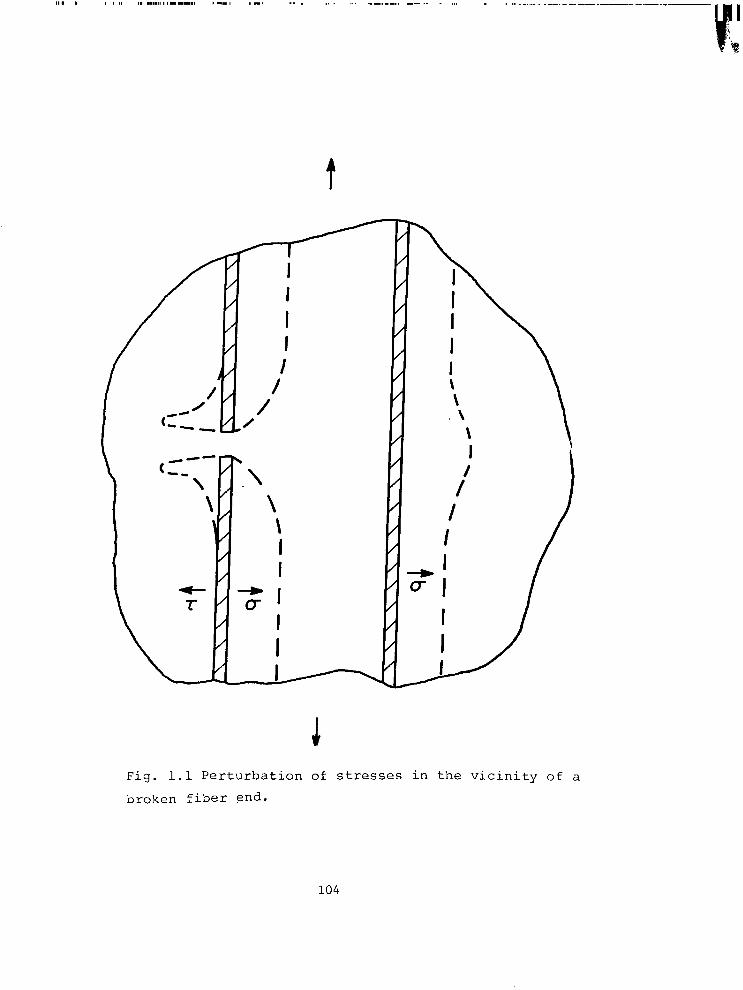
t

( e--- -a

\

\i \

, /

/

T ’ /

I I I I \ \ \ \ I

; I

I

Fig. 1.1 Perturbation of stresses in the vicinity of a

broken fiber end.

104

600

500

4lxl

3oc

20[

KM i

I I

I I

I I

1 2

5 10

20

50

GAG

E LEN

GTH

, IN.

Fig.

1.

2 Va

riatio

n of

m

ean

and

rang

e of

in

divi

dual

fib

er

stre

ngth

va

lues

. (B

oron

fib

er

data

frp

m

Ref.

1.1)

STATISTICAL TENSILE FAILURE MODEL

c Fig. 1.3 Geometry of composite for statistical tensile failure model.

106

Fig. 1.4 Distribution of damage in a fiber composite

material resultihq Tirom an applied tensile load.

107

N=l (

20)

- e=

o ---

6=

0!

I

2.0

I 3.0

LOAD

RATI

O, P

/Py

I I

% 0

5.0

Fig.

2.

1 Va

riatio

n of

th

e lo

ad

conc

entra

tion

fact

or

in

the

first

un

brok

en

fiber

wi

th

the

ratio

of

ap

plie

d lo

ad

to

limit

load

fo

r va

rious

va

lues

of

th

e po

st-fa

ilure

sh

ear

stre

ss

ratio

, r-i

. (O

ne b

roke

n fib

er

- 2D

arra

y).

5.0

4.0

3.0

2.0 1.0

0.0

N=l(2

D)

1.0

3.0

LOAD

RAT

IO, P

/Py

Fig.

2.

2 Va

riatio

n of

th

e br

oken

fib

er

leng

th

alon

g wh

ich

the

shea

r st

ress

es

are

inel

astic

wi

th

the

ratio

0:

ap

plie

d lo

ad

to

limit

load

fo

r va

rious

va

lues

of

th

e po

st-fa

ilure

sh

ear

stre

ss

ratio

, 11

. (O

ne b

roke

n fib

er

- 2D

arra

y).

3.0

2.5

2.0

1.5

1.0

0.5 1.

0

N=lO

(20)

-

f=o

w--

E&Y

‘. I--

,~

mm

gBb_

-aM

l--~~

~---

-

---

----

1.0

2.0

3.0

LOAD

RAT

IO, P

IPy

4.0

5.0

Fig.

2.

3 Va

riatio

n of

th

e lo

ad

conc

entra

tion

fact

or

in

the

first

un

brok

en

fiber

wi

th

the

ratio

of

ap

plie

d lo

ad

to

limit

load

to

va

rious

va

lues

of

th

e po

st-fa

ilure

sh

ear

stre

ss

ratlo

, rl.

(T

en b

roke

n fib

ers

- 2D

arra

y).

4.0

0 i=

r 2

2.0

P iii z

1.0

0.0

i. o-

LOAD

RAT

IO, P

IPy

Fig.

2.

4 Va

rlatlo

n of

tn

e br

oken

fib

er

leng

th

alon

g wh

ich

the

shea

r st

ress

es

are

inel

astic

wi

th

the

ratio

of

ap

plie

d lo

ad

to

limit

load

fo

r va

rious

va

lues

of

th

e po

st

failu

re

shea

r st

ress

ra

tio,

II.

(Ten

bro

ken

fiber

s -

2D a

rray)

,

N=lO

O (2

D)

- t=

o ---

&C

l!

1.0

1.0

2.0

3.0

LOAD

RAT

IO, P

IP Y

Fig.

2.

5 Va

riatio

n of

th

e lo

ad

conc

entra

tion

faci

xr

in

the

first

un

brok

en

fiber

wi

th

the

ratio

of

ap

plie

d lo

ad

to

limit

load

fo

r va

rious

va

lues

of

th

e po

st-fa

ilure

sh

ear

stre

ss

ratio

, rl.

(1

00

brok

en

fiber

s -

2D a

rray)

.

5.0

4.0

3.0

2.0 1.0

0.0

1.0

N=lO

O (2

D)

2.0

LOAD

RATI

O, P

/Py

r2.g

. 2.

6 Va

riatio

n of

th

e br

oken

fib

er

leng

th

alon

g wh

ich

the

shea

r st

ress

es

are

inel

astic

wi

th

the

ratio

of

ap

plie

d lo

ad

to

limit

load

fo

r va

rious

va

lues

of

th

e po

st-

failu

re

shea

r st

ress

ra

tio,

rl.

(100

bro

ken

fiber

s -

2D a

rray)

.

5.0

4.0

3.0

2,o

1.0

0.0

I I

I I

1.0

1.1

1.2

1.3

1.4

1.5

LOAD

RATI

O, P

/Py

1.6

1.7

1.8

Fig.

2.

7 Va

riatio

n of

th

e br

oken

fib

er

leng

th

alon

g wh

ich

the

shea

r st

ress

es

are

inel

astic

wi

th

the

ratio

of

ap

plie

d lo

ad

to

limit

load

fo

r va

rious

va

lues

of

th

e po

st-fa

ilure

sh

ear

stre

ss

ratio

, rl.

(T

wo b

roke

n fib

ers

- 2D

arra

y).

N=l (

SQUA

RE AR

RAY)

1.15

1.10

1.05

1.00

0.95

g=0

--w

(=Cr

-s--m

&-

=c---

----

---Bm

wB-

-m

1.0

I I

I J

1.0

2.0

3.0

4.0

LOAD

RATI

O, p

/py

Fig.

2.

8 Va

riatio

n of

th

e lo

ad

conc

entra

tion

fact

or

in

the

first

un

brok

en

fiber

wi

th

the

ratio

of

ap

plie

d lo

ad

to

limit

load

fo

r va

rious

va

lues

of

th

e po

st-fa

ilure

sh

ear

stre

ss

ratio

, IJ

. ar

ray)

. (O

ne b

roke

n fib

er

- 3D

squ

are

500

40

a g 3.

0 25

J 0,

G

3

2.0

E

1.0

000

N=l (

SQUA

RE AR

RAY)

LOAD

RATI

O, P

/P Y

Fig.

2.

9 Va

riatio

n of

th

e br

oKen

fk

ber

leng

th

alon

g wh

ich

the

shea

r st

ress

es

are

inel

astic

wi

th

the

ratio

of

ap

plie

d lo

ad

to

limit

load

fo

r va

rious

va

lues

of

th

e po

st-

failu

re

shea

r st

ress

ra

tio,

11.

(One

bro

ken

fiber

-

3D

squa

re

ayya

v1.

1.40

r N

=9(S

QU

AREA

RR

AY)

E=O

---

E/Y

I I

I P

1.0

2.0

3-o

4.0

5.0

LOAD

RAT

\O, P

IPy

Fig.

2.

10

Varia

tion

of

the

load

co

ncen

tratio

n fa

ctor

in

th

e fir

st

unbr

oken

fib

er

with

th

e ra

tio

of

appl

ied

load

to

lim

it lo

ad

for

vario

us

valu

es

of

the

post

-failu

re

shea

r st

ress

ra

tio,

I-I.

(Nin

e br

oken

fib

ers

- 3D

squ

are

arra

y).

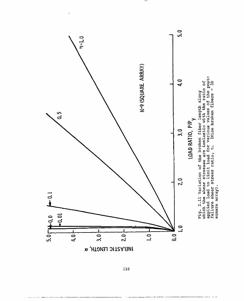
5.0

4.0

u . E a 5 3.

0

2 !7l

4 w

2,o

5

a. 0

0.0

-0.0

0.

1

t /

co. 0

1

N=9

(SQ

UAR

E AR

RAY

.)

1.0

2.0

3.0

4,o

LOAD

RAT

IO, P

/Py

Fig.

2.

11

Varia

tion

of

the

brok

en

fiber

le

ngth

al

ong

whic

h th

e sh

ear

stre

sses

ar

e in

elas

tic

with

th

e ra

tio

of

appl

ied

load

to

lim

it lo

ad

for

vario

us

valu

es

of

the

post

- fa

ilure

sh

ear

stre

ss

ratio

, n.

(N

ine

brok

en

fiber

s -

3D

squa

re

arra

y).

0.6

Kl

= 1.

333

K10

4.97

K50

= 6.3

4

I= N

UM

BER

OFB

RO

KEN

FI

BER

S

1 2

3 4

5 6

7 8

9 10

11

12

13

14

15

DIS

TAN

CE F

RO

MLA

STBR

OKE

N

FIBE

R, J

Fig.

2.

12

Ratio

of

lo

ad

incr

ease

in

un

brok

en

fiber

s to

th

e lo

ad

incr

ease

in

th

e fir

st

unbr

oken

fib

er

for

vario

us

num

bers

of

br

oken

fib

ers.

1 2

3 4

5 67

8

9 10

CR

ACK S

IZE,

N

Fig.

2.

13

Varia

tion

of

elas

tic

inef

fect

ive

leng

th

with

cr

ack

size

fo

r 2D

fib

er

arra

y.

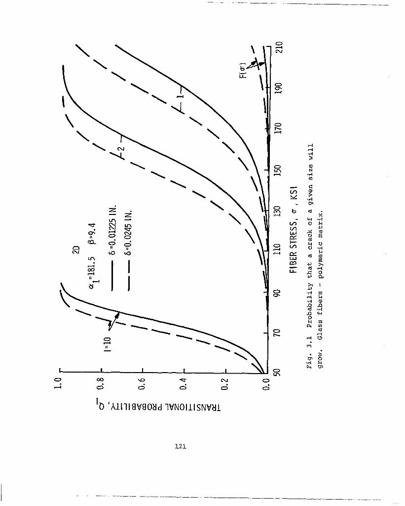
1.0

0.8

0.6

0.4

0.2

0.0

- 6=

0.01

225 I

N.

-- 6=

0.02

45 IN

.

50

70

90

110

130

150

170

190

210

FIBE

R ST

RES

S, u,

KS

I Fi

g.

3.1

Prob

abili

ty

that

a

crac

k of

a

give

n si

ze

will

grow

. G

lass

fib

ers

- po

lym

eric

m

atrix

.

1.0

0.8

0.6

0.4

0.2

0.0

. TF

11

0 /

-- 2D

I

. I --

blCO

NSTA

NT

- ~Q

VARI

ABLE

/

I

I 3

= 18

1.5

P= 9

.4

. 6,

=‘0.

0122

5 IN

.

I I

I I

50

70

90

110

130

150

170

190

210

FIBE

R ST

RESS

, u,

KSI

Fig.

3.

2 Ef

fect

of

ch

ange

in

el

astic

in

effe

ctiv

e le

ngth

wi

th

crac

k si

ze

upon

tra

nsiti

onal

pr

obab

ilitie

s.

Gla

ss

fiber

s -

poly

mer

ic

mat

rix.

0.8

0.6

0.4

0.2

0.0

f

/

- y=

17

6.8,

p

=15.

0

--al=

18

6.9,

p=

5.0

/

/

/ 1 FW

) hl

= 0.

0122

5 IN

.

’ l

50

90

130

170

210

250

290

330

FIBE

R ST

RESS

, u,

KSI

Fig.

3.

3 Ef

fect

of

fib

er

stre

ngth

di

sper

sion

up

on

trans

ition

al

prob

abilit

ies

for

two

glas

s fib

er

popu

latio

ns

havi

ng

the

sam

e m

ean

stre

ngth

fo

r a

one

inch

te

st

leng

th.

1.0

-

BORO

N-EP

OXY

al=

470.

0 /3

=8.8

2

6= 0

.025

IN.

2 3D

-2D

/

/

/

0.0

260

300

340

380

420

460

500

NOM

INAL

FIBE

R ST

RESS

, KSI

Fig.

3.

4 co

mpa

rison

of

tra

nsiti

onal

pr

obab

ilitie

s fo

r 2D

and

?D

fib

er

arra

ys.

Boro

n fib

ers

- ep

oxy

mat

rix.

0.8

0.6

0.4

0.2

0.0

~~“1

81.5

f3

=9.4

6 =O

. 0122

5 IN.

M=8

0 N=l

OO

/

/

100

120

140

160

180

Fl B

ER ST

RESS

, c ,

KS I

Fig.

3.

5 Co

mpa

rison

of

tra

nsiti

onal

pr

obab

ilitie

s fo

r 2D

and

3D

fiber

ar

rays

. G

lass

fib

ers

- ep

oxy

mat

rix.

2D

al = 181.5 P=9.4

190 bl= 0.01225 IN.

150

130

110 X

0.99 90 0.9

0. 8

0.5 70 .

0.1

50 I I I I I I I I I

1 2 3 4 5 6 7 8 9 10

CRACK SIZE, I Fig. 3.6 Variation with crack size of the stress required for a given transitional probability.

126

1.0

0.8

0.6

0.4

0.2

0.0

~1=1

81.5

50

70

90

110

130

150

170

FIBE

R STR

ESS,

r , K

SI

Fig.

3.

7 Pr

obab

ility

of

havi

ng

a cr

ack

of

a gi

ven

size

as

a fu

nctio

n of

st

ress

. G

lass

fib

ers,

ep

oxy

mat

rii,

2D

arra

y.

LO

I=1

0,9

0. 8

Y

BORO

N-EP

OXY

(3D)

0.7

~1'4

70

(3=8

.82

6= 0

.025

IN.

oh

- M

=120

, N=6

24

0.5

-

0.4

-

0.3

-

0.2

-

0, 1

0.0

240

280

320

360

400

440

480

FIBE

R ST

RESS

, KSI

Fig.

3.

8 Pr

obab

ility

of

havi

ng

a cr

ack

of

a gi

ven

size

as

a fu

nctio

n of

st

ress

. Bo

ron

fiber

s,

epox

y m

atrix

, 3D

ar

ray.

210

190

170

150

130

110

90

70

50

“1’181.5 p = 9.40

b;0.01225 IN.

N=lOO

/ CUMULATIVE GROUP MODE

P,=O. 99 M

lo*

1 2 3 4 5 6 7 8 9 10 CRACK SIZE, I

Fig. 3.9 Stress levels for various events contributing to composite failure. (2D reference glass/epoxy composite).

129

230

210

190

170

150

130

110

90

70

-IBER BREAK PROPAGATION 2D

-Q,= 0.99 y=181.5 I3 =9.4

6 =O. 0245 IN.

CUMULATIVE GROUP

MATRIX FAILURE

I I I 1 I I I I I

1 2 3 4 5 6 7 8 9 10

M 10

ld

ld

lo4

ld

lo6

CRACK SIZE, I Fig. 3.10 Stress levels for various events contributing to composite failure. (2D glass/epoxy with increased ineffective length).

130

3

210

190

170

I.50

130

110

90

7cl

50

MATRIX FAILURE

6;=0.01225 IN.

1 2 3 4 5 6 7 8 9 10

10’

M

ld

lo4

ld

lo6

CRACK SIZE, I Fig. 3.11 Stress levels for various events contributing to composite failure. (2D glass/epoxy with fibers having a greater dispersion of strength).

131

- m

b

cx W m - Ll-

140

120

CUMULATIVEGROUP MODE CUMULATIVEGROUP MODE

\ MATRIX FAIL \ MATRIX FAIL al=181,5 p=9,.4 \ al=181,5 p=9,.4 \

b =O, 01225 IN.

Id =lOO

T =lO,OKSl Y

I I I l , I ,

I I 1 I I I

1 2 3 4 5 6 7 8 9 10

CRACK SIZE, I

.URE

Fig. 3.12 Stress levels for various events contributing

to composite failure.(3D reference glass/epoxy composite).

132

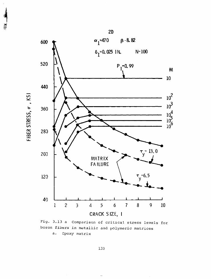
2D

600

520

360

283

203

123

40

Fig.

al=470 p-a82

\ 61=OJ25 IN. N=lOO

I I I I I I I I I

1 2

3.13 a

3 4 5

CRACK Comparison of

6 7 8 9 10

SIZE, I

critical stress levels for boron fibers in metallic and polymeric matrices

a. Epoxy matrix

133

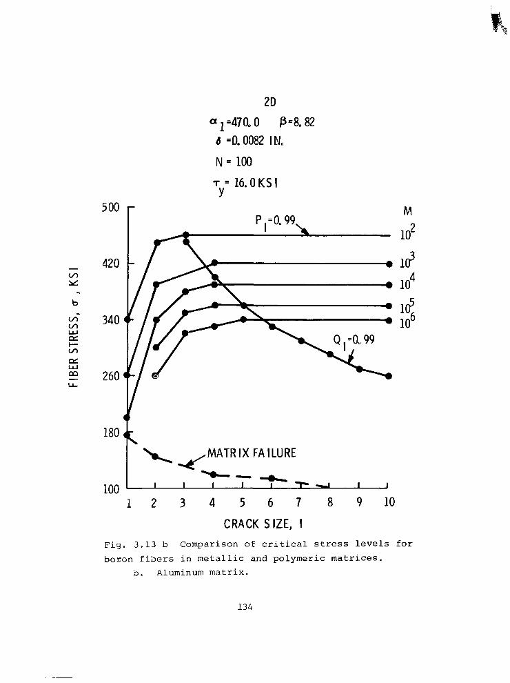
420

260

180

2D

y=470.0 P=8.82 d =a0082 INo

N = 100

Ty= 16.OKSl

- -- M P,=O. 99, 3

b k -6

MATRIX FAILURE

1 2 3 4 5 6 7 8 9 10

CRACK SIZE, I

Fig. 3.13 b Comparison of critical stress levels for

boron fibers in metallic and polymeric matrices. b. Aluminum matrix.

134

520 ,

480

440

400

360

280

I 240

200

- T

1 a,= 470 /3=8.82

1

6 = 0,025 IN.

N= 624

i-

MATRIX FAILURE

I I 1 I I I I I

12 3 4 5 6 7 8 9 10

CRACK SIZE, I Fig. 3.14 Stress levels for various events contributing

to composite failure. (3D boron/epoxy composite).

135

230

210

190

170

I.50

130

110

lo2

dl= 0,01225 IN.

dl= OoO1225 IN

$= 0.0245 IN.

2D

(1) y=186.9, p= 5.0,

N= 100

ld lo4 105 lo6

NUMBER OF LAYERS. N Fig. 3.15 Change in stress level for fiber break propagation mode with sample size for various glass/

polymer composites.

136

280

260

240

220

200

180

160

140

120 1

L-FIBER BREAK

CUMULATIVEGROUP MODE

DEBOND 7 =lOksi

Y

2 3

GROUP SIZE

Fig. 3.16 Average fiber stress for various elastic

failure events (2D glass/epoxy composites).

137

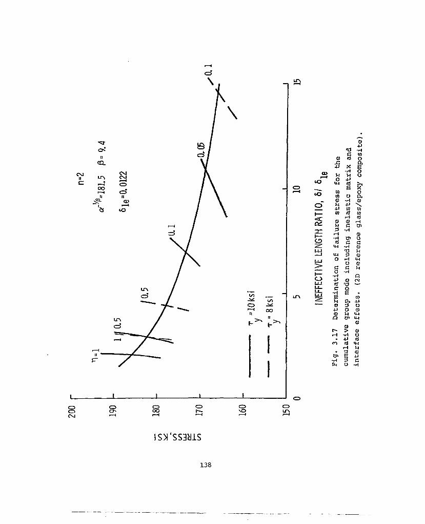
n=2

a'+=

181.

5 p=

9.4

61e"

O. 0

122

, 'Y

=lO

ksr

- -

T =

8ksi

Y

I I

J

160

150

0 5

10

l5

INEF

FECT

IVE LE

NGTH

RATI

O, 6

1 Q

Fi

g.

3.17

De

term

inat

ion

of

failu

re

stre

ss

for

the

cum

ulat

ive

grou

p m

ode

incl

udin

g in

elas

tic

mat

rix

and

inte

rface

ef

fect

s,

(2D

refe

renc

e gl

ass/

epox

y co

mpo

site

),

180

i70

160

I50

~t-‘~

=181

.5

f3=9

.4

Sle=

0.01

225

n=2

/ I

I I

I I

I I

I I

0. 0

0.2

0.6

POST

-FAI

LURE

SHEA

R STR

ESS R

ATIO

, '-I

= 71

I- Y

Fig.

3.

18

Influ

ence

of

m

atrix

/inte

rface

fa

ilure

-stre

ss

leve

l an

d po

st-fa

ilure

m

atrix

sh

ear

trans

fer

upon

co

mpo

site

st

reng

th.

(2D

refe

renc

e gl

ass/

epox

y co

mpo

site

).

1.0

190

180

170

160

150

140 1 2 3 4 5

REFERENCE GROUP SIZE

Fig. 3.19 Influence or characteristic group size upon computed failure stress in the cumulative group mode. (2D reference glass/epoxy composite).

140

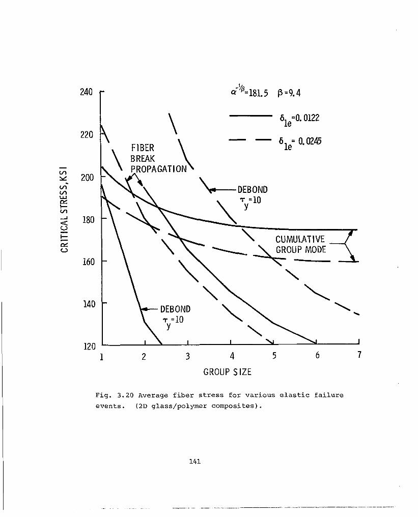
240 [email protected] @=9.4

220 \

\

\ FIBER \

61e=o. 0122

-- %? = 0,0245

200 \

BREAK \

\ PROPAGATION \

'e-DEBOND

180

160

140

120

I

t

DEBOND \ \ 7 =lO Y

1 3 4 5 6 7

GROUP SIZE

Fig. 3.20 Average fiber stress for various elastic failure events. (2D glass/polymer composites).

141

.-. _. -- _ -~ -. --_---- I_--- ~------

0

220

210

200

190

180

170

160

l.50

.

N=2

? =

6.0

%

=9.0

245

%?

, = 0,

0122

I

I I

I I

I I

I 0,

2 0.

4 0.

6 0.

8

POST

FAIL

UR

E SH

EAR

STR

ESS R

ATIO

, ? =

T/T

Y

1.0

Fig.

3.

21

Influ

ence

of

fib

er

and

mat

rix

prop

ertie

s up

on

com

posi

te

stre

ngth

(b

ased

on

fib

er

area

).

E

n=l

c+=1

86.9

p

=5.0

%e =

0.01

22

rY =

10ks

i

I I

I 3

0 5

10

l5

INEF

FECT

IVE LE

NG

TH RA

TIO

, 61

$ Fi

g.

3.22

De

term

inat

ion

of

failu

re

stre

ss

for

the

cum

ulat

ive

grou

p m

ode

incl

udin

g in

el,a

stic

m

atrix

an

d in

terfa

ce

effe

cts.

(2

D gl

ass/

epox

y wi

th

fiber

s ha

ving

a

grea

ter

disp

ersi

on

of

stre

ngth

).

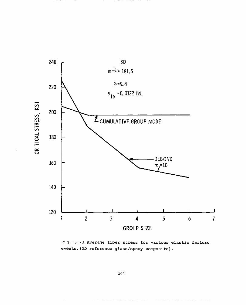
240

220

200

180

160

140

120

3D a-‘/p= 181.5

p=9,4

% =0.012'2 IN.

1 2 3 4 5 6 7

GROUPSIZE

Fig. 3.23 Average fiber stress for various elastic failure events.(3D reference glass/epoxy composite).

144

200

170

3D

N=2

(r-I/p

=181

.5

p=9.

4

%e =

0,01

22

Ty=

10

160

0 5

10

INEF

FECT

IVE LE

NGTH

RATI

O,

W

die

I5

Fig.

3.

24

Dete

rmin

atio

n of

fa

ilure

st

ress

fo

r th

e cu

mul

ativ

e gr

oup

mod

e in

clud

ing

inel

astic

m

atrix

an

d in

terfa

ce

effe

cts.

(3

D re

fere

nce

glas

s/ep

oxy

com

posi

te

with

X=

2).

3D

200 170

Ml

N=3

a-'@

=181

.5

p=9.

4

I I

I ,t-

5 10

l.2

INEF

FECT

IVE LE

NGTH

RATI

O,

” Ye

0

Fig.

3.

25

Dete

rmin

atio

n of

fa

ilure

st

ress

fo

r th

e cu

mul

ativ

e gr

oup

mod

e in

clud

ing

inel

astic

m

atrix

an

d in

terfa

ce

effe

cts.

(3

D re

fere

nce

glas

s/ep

oxy

com

posi

te

with

IV

= 3

).

500

450

400

350

a-“~=470 p =8.Q

‘le = 0.025

CUMULATIVE GROUP MODE

DEBOND 7 =lO Y

FIBER BREAK PROPAGATION qi= 0,99

1 2 3 4 5 6 7

GROUPSIZE

Fig. 3.26 Average fiber stress for various elastic failure events. (2D boron/epoxy composite,)

147

500

480

420

400

0

n=2

-"'=4

70

Q

P =8

.82

‘le =

0,02

5 TY

= 10

ksi

5 10

INEF

FECT

IVE LE

NGTH

RATI

O, 6

/ hl

e

Fig.

3.

27

Dete

rmin

atio

n of

fa

ilure

st

ress

fo

r th

e cu

mul

ativ

e gr

oup

mod

e in

clud

ing

inel

astic

m

atrix

an

d in

terfa

ce

effe

cts.

(2

D bo

ron/

epox

y co

mpo

site

).

500

350

300

0

3D

N=l

a-‘=

470

f3 =8

,82

%e =

0,02

5 ;=

6,5

5

INEF

FEC

TIVE

LE

NG

TH RAT

IO, S

l bl

e

Fig.

3.

28

Dete

rmin

atio

n of

fa

ilure

st

ress

fo

r th

e cu

mul

ativ

e gr

oup

mod

e in

clud

ing

inel

astic

m

atrix

an

d in

terfa

ce

effe

cts.

(3

D bo

ron/

epox

y co

mpo

site

).

550

500

400

3D

N=l

a-b=

316

p =(

j,4

%e

= 0.

0017

2 TY

=4* O

0 5

10

I.5

INEF

FECT

IVE LE

NGTH

RATI

O, 6

1 til

e

Fig.

3.

29.

Dete

rmin

atio

n of

fa

ilure

st

ress

fo

r th

e cu

mul

ativ

e gr

oup

mod

e in

clud

ing

inel

astic

m

atrix

an

d in

terfa

ce

effe

cts.

(3

D ca

rbon

/epo

xy

com

posi

te).

OVE

RSTR

ESSE

D RE

GIO

N

REG

ION O

FMAT

RIX

FAIL

URE

CR

ACK

Fig.

4.

1 Sc

nem

atic

re

pres

enta

tion

of

the

effe

ct

of

a pr

e-ex

istin

g cr

ack

in

a co

mpo

site

un

der

tens

ile

load

.

ELASTIC MATRIX

INELASTIC MATRIX ZONE

F 'ig. B.l Approximate model for the evaluation of stresses i .n a 2D composite with inelastic matrix effects-

AVERAGE n

COREOFBROKEN

MATE,RIAL FIBERS

t UNBROKEN FIBER

153

.-~. _--- -

1.35

1.30

1.25

1.20

1.15

1. 10

1.05

1.00

N=l (2D) rl=l. 0

INF IN ITE ARRAY

- - - APPROXIMATE MODEL

\

\

\ \

1.0 3.0 5.0 7*0 LOAD RATIO, P/P

Y

9.0 11,o

Fig. 13.2 Comparison of load concentratiofi factors from the approximate 2D inelastic model with those for the infinite array.

154

. - _ __ __---. - .-- ------- -- -.- - -_

1.35

L30

1.25

1.20

1.15

1.10

1.05

0.0

N=l CD) q=o. 0

INFINITE ARRAY

-- - APPROXIMATE MODEL

\

1.00 1.02 1.04 1.06 1.08 1.10

LOAD RATIO, PIP Y

Fig. B.3 Comparison of load concentration factors from the approximate 2D inelastic model with those for the infinite array in the case of no post-failure shear stress transfer.

155

__ .--__I.- ~- - --___

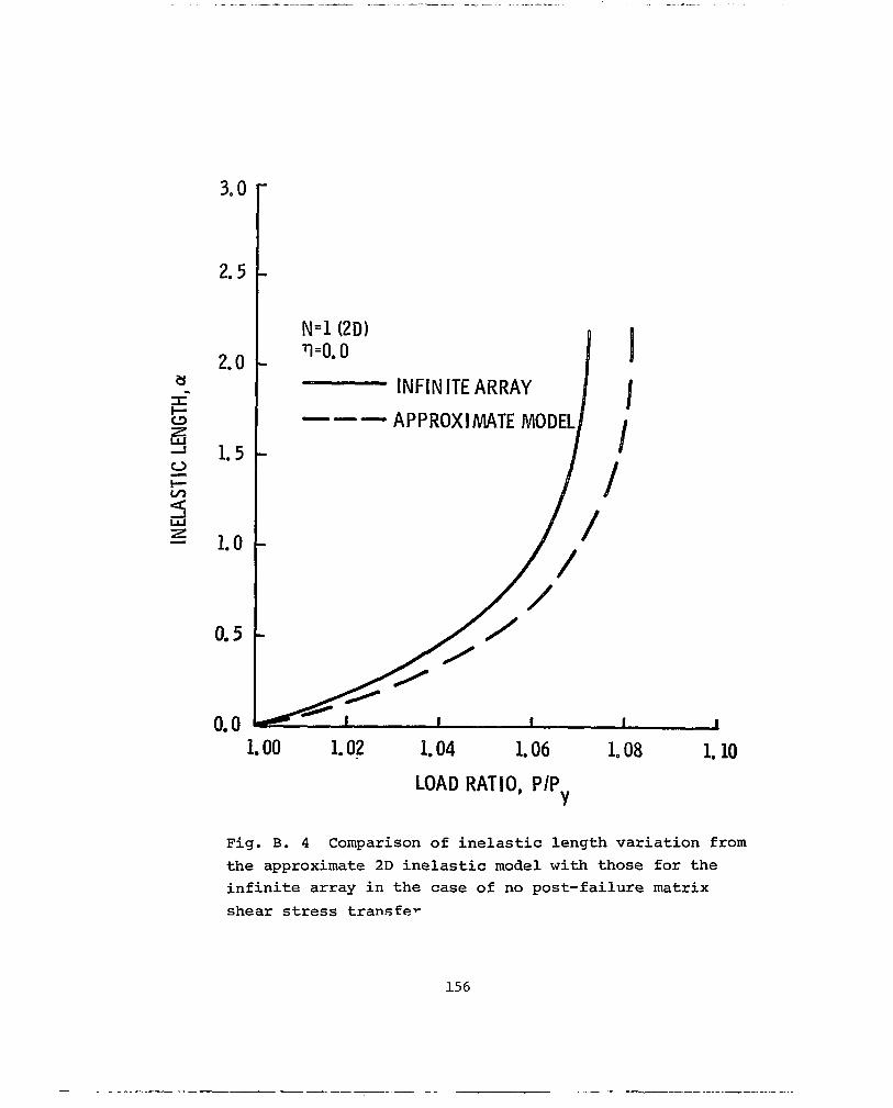
3.0

2. 5

2.0

1. 5

1.0

0.5

0.0 1.00

N=l(ZD) rl=o. 0

INFINITEARRAY ---APPROXIMATEMODEL

I

1. O? 1.04 1.06 1.08 LOAD RATIO, P/Py

Fig. B. 4 Comparison of inelastic length variation from the approximate 2D inelastic model with those for the infinite array in the case of no post-failure matrix shear stress transfer

156

------__---_ .--- .__-. -.- -.

ELASTIC MATRIX

MATRIX ZONE

&ORE OF BROKEN FIBERS

RING OF INTACT FIBERS

AVERAGE MATER IAL Fig. B.5 Approximate model for the evaluation of st in a 3D model of a unidirectional composite with ine matrix effects.

resses lastic

157

1.4

1.2

1.0

0.4

0.2

0.0

INFINITE ARRAY w - - APPROXIMATE MODEL

N=l ?=O. 0 SQUARE ARRAY

n I I I

I /

J

LOAD RATIO, PIPy

Pig. B.6 Comparison of inelaSriC length variation from the

approximate 3D inelastic -ode1 with those for the infinite

array in the case of no post-failure matrix shear stress

transfer.

158

1. 12

1.08

1.06

1.04

1.02

1.00

INFINITE ARRAY

---APPROXIMATEMODEL

N=l (HEXAGONALARRAY) 'I= 0.0

\

\

\

\

1.00 1.01 1.02 1.03

LOAD RATIO. PIP Fig. B.7 Comparison of load concentration factors from the approximate 3D hexagonal array inelastic model with those for the infinite array in the case of no post- failure matrix shear stress transfer.

159

1. 16

1.08

1.06

1.04

1.02

1.00

INFINITE ARRAY \

-- - APPROXIMATE MODEL \

1.00 1.01 1.02 1.03 1.04 1.05

LOAD RATIO, PIP V

Fig. B.8 Comparison of load concentrakon factors from the approximate 3D square array inelastic model with those for the infinite array in the case of no post-failure matrix

shear stress transfer.

160

1. 16

1.14

0’ 1.10

5 E 5 g 1.08 0 0 2 2

1.06

1.04

N=l (SQUARE ARRAY) rl=l. 0

INFINITE ARRAY --- APPROXIMATE MODEL

1.0 2.0 3.0 4.0 5.0 6.0 LOAD RATIO, PIPy

Fig. B.9 Comparison of load concentration factors from the approximate 3D square array inelastic.model with those for the infinite array.

161

0.9

I I

I I

I I

I I

0 0.

2 0.

4 0.

6 0.

8 1.

0 1.

2 1.

4 1.

6 D

ISTA

NC

EALO

NG

FIBE

R,t

Fig.

C.

l Va

riatio

n of

lo

ad

in

first

un

brok

en

fiber

ad

jace

nt

to

a si

ngle

br

oken

fib

er.

tensile failure criteria for fiber composite materials · 2013-08-31 · tensile failure criteria...

Documents