ten chapters of the algebraical art - qmul mathspjc/notes/intalg.pdf · ten chapters of the...
TRANSCRIPT
Ten Chapters of theAlgebraical Art
Peter J. Cameron

ii
Preface
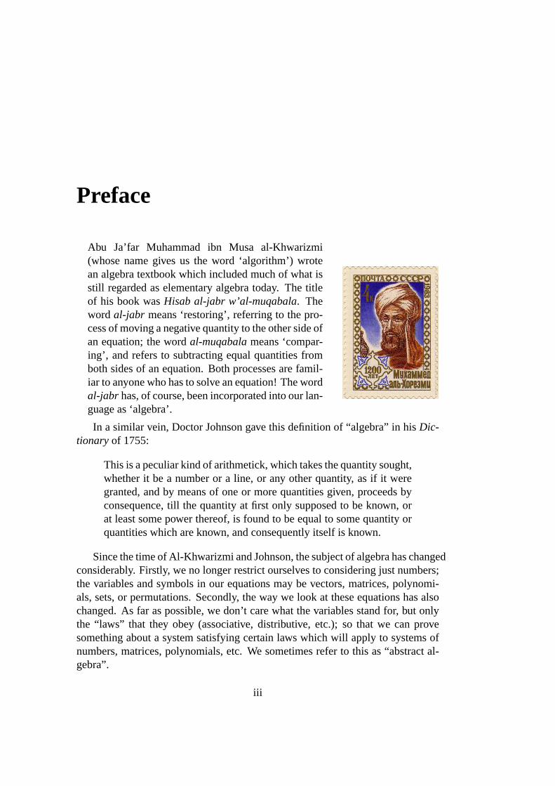
Abu Ja’far Muhammad ibn Musa al-Khwarizmi(whose name gives us the word ‘algorithm’) wrotean algebra textbook which included much of what isstill regarded as elementary algebra today. The titleof his book wasHisab al-jabr w’al-muqabala. Theword al-jabr means ‘restoring’, referring to the pro-cess of moving a negative quantity to the other side ofan equation; the wordal-muqabalameans ‘compar-ing’, and refers to subtracting equal quantities fromboth sides of an equation. Both processes are famil-iar to anyone who has to solve an equation! The wordal-jabr has, of course, been incorporated into our lan-guage as ‘algebra’.
In a similar vein, Doctor Johnson gave this definition of “algebra” in hisDic-tionaryof 1755:
This is a peculiar kind of arithmetick, which takes the quantity sought,whether it be a number or a line, or any other quantity, as if it weregranted, and by means of one or more quantities given, proceeds byconsequence, till the quantity at first only supposed to be known, orat least some power thereof, is found to be equal to some quantity orquantities which are known, and consequently itself is known.
Since the time of Al-Khwarizmi and Johnson, the subject of algebra has changedconsiderably. Firstly, we no longer restrict ourselves to considering just numbers;the variables and symbols in our equations may be vectors, matrices, polynomi-als, sets, or permutations. Secondly, the way we look at these equations has alsochanged. As far as possible, we don’t care what the variables stand for, but onlythe “laws” that they obey (associative, distributive, etc.); so that we can provesomething about a system satisfying certain laws which will apply to systems ofnumbers, matrices, polynomials, etc. We sometimes refer to this as “abstract al-gebra”.
iii

iv
These notes are intended for the course MAS117,Introduction to Algebra, atQueen Mary, University of London. The course is to be given for the first time inthe spring semester of 2007.
The course is intended as a first introduction to the ideas of proof and abstrac-tion in mathematics, as well as to the concepts of abstract algebra (groups andrings). TheUndergraduate Studies Handbooksays:
This module is an introduction to the basic notion of algebra, such assets, numbers, matrices, polynomials and permutations. It not onlyintroduces the topics, but shows how they form examples of abstractmathematical structures such as groups, rings, and fields and how al-gebra can be developed on an axiomatic foundation. Thus, the notionsof definitions, theorem and proof, example and counterexample aredescribed. The course is an introduction to later modules in algebra.
The course replaces the earlier courseDiscrete Mathematics, with which itshares some material. But since it is a new course, I have re-written the notesfrom scratch. Of course, these notes arenot a substitute for the lectures!
The exercises at the ends of the chapters vary in difficulty from routine tochallenging. To a first approximation, the easier exercises come first.
If you enjoyed this course, the next step is MAS201,Algebraic Structures I.You can also find a set of notes for this course on my web page.
This set of notes is a slightly revised version of the notes which were availableduring the course. I am grateful to Matilda Okungbowa for a number of correc-tions.
Note: The pictures and information about mathematicians in these notes aretaken from the St AndrewsHistory of Mathematicswebsite:http://www-groups.dcs.st-and.ac.uk/~history/index.html
Peter J. Cameron25 June 2007

Contents
1 What is mathematics about? 11.1 Some examples of proofs . . . . . . . . . . . . . . . . . . . . . . 11.2 Some proof techniques . . . . . . . . . . . . . . . . . . . . . . . 61.3 Proof by induction . . . . . . . . . . . . . . . . . . . . . . . . . 71.4 Some more mathematical terms . . . . . . . . . . . . . . . . . . . 10
2 Numbers 152.1 The natural numbers . . . . . . . . . . . . . . . . . . . . . . . . 162.2 The integers . . . . . . . . . . . . . . . . . . . . . . . . . . . . . 172.3 The rational numbers . . . . . . . . . . . . . . . . . . . . . . . . 182.4 The real numbers . . . . . . . . . . . . . . . . . . . . . . . . . . 192.5 The complex numbers . . . . . . . . . . . . . . . . . . . . . . . . 192.6 The complex plane, or Argand diagram . . . . . . . . . . . . . . 21
3 Other algebraic systems 253.1 Vectors . . . . . . . . . . . . . . . . . . . . . . . . . . . . . . . 253.2 Matrices . . . . . . . . . . . . . . . . . . . . . . . . . . . . . . . 283.3 Polynomials . . . . . . . . . . . . . . . . . . . . . . . . . . . . . 313.4 Sets . . . . . . . . . . . . . . . . . . . . . . . . . . . . . . . . . 32
4 Relations and functions 354.1 Ordered pairs and Cartesian product . . . . . . . . . . . . . . . . 354.2 Relations . . . . . . . . . . . . . . . . . . . . . . . . . . . . . . 374.3 Equivalence relations and partitions . . . . . . . . . . . . . . . . 374.4 Functions . . . . . . . . . . . . . . . . . . . . . . . . . . . . . . 404.5 Operations . . . . . . . . . . . . . . . . . . . . . . . . . . . . . . 434.6 Appendix: Relations and functions . . . . . . . . . . . . . . . . . 44
5 Division and Euclid’s algorithm 475.1 The division rule . . . . . . . . . . . . . . . . . . . . . . . . . . 475.2 Greatest common divisor and least common multiple . . . . . . . 48
v

vi CONTENTS
5.3 Euclid’s algorithm . . . . . . . . . . . . . . . . . . . . . . . . . . 495.4 Euclid’s algorithm extended . . . . . . . . . . . . . . . . . . . . 505.5 Polynomials . . . . . . . . . . . . . . . . . . . . . . . . . . . . . 51
6 Modular arithmetic 556.1 Congruence modm . . . . . . . . . . . . . . . . . . . . . . . . . 556.2 Operations on congruence classes . . . . . . . . . . . . . . . . . 566.3 Inverses . . . . . . . . . . . . . . . . . . . . . . . . . . . . . . . 576.4 Fermat’s Little Theorem . . . . . . . . . . . . . . . . . . . . . . 58
7 Polynomials revisited 617.1 Polynomials over other systems . . . . . . . . . . . . . . . . . . 617.2 Division and factorisation . . . . . . . . . . . . . . . . . . . . . . 627.3 “Modular arithmetic” for polynomials . . . . . . . . . . . . . . . 637.4 Finite fields . . . . . . . . . . . . . . . . . . . . . . . . . . . . . 667.5 Appendix: Laws for polynomials . . . . . . . . . . . . . . . . . . 67
8 Rings 698.1 Rings . . . . . . . . . . . . . . . . . . . . . . . . . . . . . . . . 698.2 Examples of rings . . . . . . . . . . . . . . . . . . . . . . . . . . 718.3 Properties of rings . . . . . . . . . . . . . . . . . . . . . . . . . . 718.4 Units . . . . . . . . . . . . . . . . . . . . . . . . . . . . . . . . . 748.5 Appendix: The associative law . . . . . . . . . . . . . . . . . . . 76
9 Groups 799.1 Definition . . . . . . . . . . . . . . . . . . . . . . . . . . . . . . 799.2 Elementary properties . . . . . . . . . . . . . . . . . . . . . . . . 799.3 Examples of groups . . . . . . . . . . . . . . . . . . . . . . . . . 809.4 Cayley tables . . . . . . . . . . . . . . . . . . . . . . . . . . . . 819.5 Subgroups . . . . . . . . . . . . . . . . . . . . . . . . . . . . . . 829.6 Cosets and Lagrange’s Theorem . . . . . . . . . . . . . . . . . . 839.7 Orders of elements . . . . . . . . . . . . . . . . . . . . . . . . . 859.8 Cyclic groups . . . . . . . . . . . . . . . . . . . . . . . . . . . . 87
10 Permutations 8910.1 Definition and representation . . . . . . . . . . . . . . . . . . . . 8910.2 The symmetric group . . . . . . . . . . . . . . . . . . . . . . . . 9010.3 Cycles . . . . . . . . . . . . . . . . . . . . . . . . . . . . . . . . 9210.4 Transpositions . . . . . . . . . . . . . . . . . . . . . . . . . . . . 9410.5 Even and odd permutations . . . . . . . . . . . . . . . . . . . . . 96

Chapter 1
What is mathematics about?
There is a short answer to this question: mathematics is aboutproofs. In anyother subject, chemistry, history, sociology, or anything else, what one expert sayscan always be challenged by another expert. In mathematics, once a statement isproved, we are sure of it, and we can use it confidently, either to build the nextpart of mathematics on, or in an application of mathematics.
1.1 Some examples of proofs
In this part of the course we are going to talk about how to prove things. Let usstart with an easy theorem.
Theorem 1.1 Let n be a natural number. Then n2 is odd if and only if n is odd.
If you know what the words in the theorem mean, you might try a few cases,to get a feel for what the theorem is about:
1 is odd 12 = 1 is odd2 is even 22 = 4 is even3 is odd 32 = 9 is odd
and so on. It seems to work. But this is not yet a proof; we are not convinced thatif you went on far enough, you might find a number for which the theorem wasnot true.
First let us read the theorem more carefully.
Natural number This means one of the counting numbers, 0,1,2,3,4, . . .. (Ar-guments still occur among mathematicians about whether 0 should count as a nat-ural number or not. This is just a matter of names, and doesn’t affect the theoremvery much. We will say that 0 is a natural number.)
1
2 CHAPTER 1. WHAT IS MATHEMATICS ABOUT?
If and only if We will come back to this later. For now, it means that, for anyvalue ofn, either the two statements “n is odd” and “n2 is odd” are both true, orthey are both false. In other words,
• if n is odd, thenn2 is odd;
• if n2 is odd, thenn is odd.
This shows us that we have two things to show, in order to prove the theorem.The first one looks fairly straightforward, but the second seems more difficult. Butwe can turn it round into something simpler. The statement
if n2 is odd, thenn is odd
is logically the same as the statement
if n is even, thenn2 is even.
So we have to prove the two statements:
• if n is odd, thenn2 is odd;
• if n is even, thenn2 is even.
So let’s try to prove them.We have one more thing to consider. What are even and odd numbers, math-
ematically speaking? An even number is one which is divisible by 2 exactly; inother words,n is even if it can be written asn = 2k for some natural numberk.An odd number is one which leaves a remainder of 1 when divided by 2; in otherwords,n is odd if it can be written asn = 2k+1 for some numberk.
So to prove the first statement, we assume thatn is an odd number, and haveto show thatn2 is an odd number. That is, we assume thatn = 2k+ 1 for somenatural numberk. Then
n2 = (2k+1)2 = 4k2 +4k+1 = 2(2k2 +2k)+1 = 2m+1,
wherem= 2k2 +2k. Son2 is odd.For the second statement, assume thatn is even, that is,n= 2k for some natural
numberk. Thenn2 = (2k)2 = 4k2 = 2(2k2) = 2m,
wherem= 2k2; son2 is even.Now we have finished the proof, and we are sure that the theorem is true for
all natural numbersn.

1.1. SOME EXAMPLES OF PROOFS 3
Now let’s use this theorem as abuilding block in a very famoustheorem, proved by Pythagoras,who has some claim to be the firstmathematician ever (that is, the firstperson to insist that mathematicalstatements must have proofs). Itwas Pythagoras who invented thewords “mathematics” and“theorem”.
Theorem 1.2 The number√
2 is irrational.
First we have to examine what the theorem means. The number√
2 is a pos-itive real numberx such thatx2 = 2. A rational number is a number that can beexpressed as a fractiona/b, wherea andb are integers, that is, natural numbers ortheir negatives.
Now my calculator tells me that√
2 = 1.414213562. If this is right, thenPythagoras is wrong, because this means that
√2 =
14142135621000000000
.
But it turns out that the calculator is wrong, because it also tells me that
(1.414213562)2 = 1.999999998944727844,
which is close to 2 but not exactly 2. Pythagoras claims that, no matter howaccurately the calculator does the sum and to how many places of decimals itexpresses the answer, it will never get the exact value of
√2.
So how did Pythagoras prove his theorem? He used another important tech-nique:
Proof by contradiction If I am trying to prove a statementP, I have succeededif I can show that the assumption thatP is false leads to a contradiction, a logicalabsurdity. For this shows thatP is not false, that is, it is true.
So we prove Pythagoras’s theorem by contradiction; we assume the falsity ofwhat we are trying to prove and head for a contradiction. That is, we assume that
√2 is rational.

4 CHAPTER 1. WHAT IS MATHEMATICS ABOUT?
That is, √2 =
mn
for some natural numbersm and n. Now, in a fraction like this, if there is acommon factor ofm andn, we can divide it out, and assume that they have nocommon factor. (For example,15
10 = 32.)
Now take our equation. Square roots are awkward; it usually simplifies anequation if you can get rid of them. We can easily do this by squaring both sidesof the equation, to get
2 =m2
n2 ,
or in other words,m2 = 2n2.
This equation tells us thatm2 is even, since it is 2k wherek = n2. Now we are ableto use Theorem 1.1, since we already proved this. Sincem2 is even, necessarilymis even; saym= 2p for some natural numberp. Substituting this into the equationgives
4p2 = 2n2,
and cancelling a factor 2 gives2p2 = n2.
Now we can “do it again”. The last equation shows thatn2 is even, so thatn iseven, sayn = 2q. So our original fraction for
√2 is
√2 =
mn
=2p2q
.
We can cancel the 2 to get a simpler fraction for√
2.But stop and remember what we are doing. We started off by saying that we
can assume thatm and n have no common factor, and we ended up with theirhaving a common factor of 2. So we have reached a contradiction.
According to the principle of proof by contradiction, our assumption that√
2is rational must be wrong, so that
√2 is irrational, as Pythagoras claimed.
Now let us have another famous example of a proof by contradiction. We willprove that the prime numbers go on for ever; there is no largest prime. (Recently,a computer search found a previously unknown prime number bigger than anyothers found so far. A journalist got the idea that they had found “the largestprime number”, and phoned one of my colleagues for a comment. What wouldyou say if this happened to you?)

1.1. SOME EXAMPLES OF PROOFS 5
This beautiful proof was discoveredby the Greek geometer Euclid, whowrote one of the world’s mostsuccessful textbooks ever, whichwas used for nearly two thousandyears.
Theorem 1.3 There are infinitely many prime numbers.
A prime number is a natural number which is divisible only by itself and 1.So 2, 3, 5 and 7 are prime numbers; 4 is not, since 4= 2×2. By convention, wesay that 1 is not a prime number, even though it satisfies the condition of havingno divisors except itself and 1; this is just a convention, and we will see the reasonfor it later. Now if the numbern is not prime, it must be divisible by some primenumber smaller thann. (Again, we will see why later. This is not meant to beobvious!)
We prove Euclid’s theorem by contradiction. That is, we assume that there areonly finitely many prime numbers. Then we can make a list of prime numbers:
p1, p2, p3, . . . , pk
are all the prime numbers.Let n be the number that we get when we multiply all of these primes together
and add 1:n = p1p2p3 · · · pk +1.
Now there are two cases to consider: eithern is prime, or it is not. We need toshow that either case leads us to a contradiction.
Casen is prime: In this case, sincep1, . . . , pk are all the primes,n must beone of them. But this is impossible, sincen is bigger than any of these primes.(Remember how we formedn.)
Casen is not prime: Thenn must have a prime factor, which must be oneof the primesp1, . . . , pk. But n is the product of all the primes plus one; so if wedivide it by any of the primesp1, . . . , pk, we get a remainder of one. So this caseis also contradictory.
So, again according to the principle of proof by contradiction, the assumptionthat there are only finitely many primes must be wrong; so there must be infinitelymany primes.

6 CHAPTER 1. WHAT IS MATHEMATICS ABOUT?
1.2 Some proof techniques
Here are some words you’ll find in statements you are asked to prove.
If, implies, sufficient The three statements
If A, thenB
A impliesB
A is a sufficient condition forB
all have the same meaning. They mean, “ifA is true, thenB is true”.Look more closely at this. How could this statement fail to be true? The only
way it could fail is if A is true andB is false. (IfA is false, then the statement iscorrect no matter whetherB is true or false.) This seems a bit odd, sometimes, solet us take an everyday example. Suppose I say to you, “If it is fine tomorrow, wewill go for a picnic.” The only situation in which my statement is false is if it isfine tomorrow and we don’t go for a picnic; if it rains tomorrow, my statement istechnically correct (though maybe not helpful!)
So how do we prove “ifA, thenB”? The obvious way is to assume thatA istrue, and deduce thatB must be true. Look back at our proof of “ifn is even, thenn2 is even” in the last section. We assume thatn is even and prove thatn2 is even.
Only if, is implied by, necessary This is exactly the reverse. The three state-ments
B only if A
A is implied byB
A is a necessary condition forB
all mean the same as “ifB, thenA”.The proof strategy, then, is to assume thatB is true, and deduce thatA must be
true.
If and only if, equivalent, necessary and sufficient We saw earlier that to say“A if and only if B” means that eitherA andB are both true, or they are both false.We also saw that there are two things we have to do to show this: “ifA, thenB”and “if B, thenA”. This agrees with what we just learned about “if” and “onlyif”. We sometimes also say “the statementsA andB are equivalent”, or “A is anecessary and sufficient condition forB”.
Now we turn to some proof techniques.

1.3. PROOF BY INDUCTION 7
Proof by contradiction We already met this idea. In order to proveA, we canassume thatA is false and deduce a contradiction (a statement that is logicallyimpossible). We saw two examples of this: the proofs of Pythagoras’ Theorem onthe irrationality of
√2, and Euclid’s theorem that there are infinitely many primes.
Proof by contrapositive This is a fancy way of saying that “A implies B” islogically equivalent to “not-B implies not-A”. We saw an example of this onpage 2. In order to prove the statement “ifn2 is even, thenn is even”, we provedinstead its contrapositive, the statement “ifn is odd, thenn2 is odd”.
Counterexamples Sometimes you will be given a general proposition, and askedwhether it is true or false.
Suppose for example you are trying to prove that some property holds forevery natural numbern. Let us call the propertyA(n). Now:
• If A(n) is true, then we have to give a general proof for it.
• If A(n) is false, we only have to give one value ofn for which it is not true.
For example, suppose we are considering the statement “every odd number isprime”. SoA(n) would be, “if n is odd, thenn is prime”. If this happened to betrue, we would have to give a proof of it. But it is false, and all we need to say is“the number 9 is odd, but is not prime since it is equal to 3×3”. In this case, wesay that 9 is acounterexampleto the statement that, ifn is odd, thenn is prime.
1.3 Proof by induction
This is a more specialised technique but is very important, so we give it a sectionto itself.
Suppose that we are trying to prove a statement about all natural numbers.Suppose thatA(n) is the statement about the particular natural numbern. Thestrategy of proof by induction is to do the following:
(a) Prove the statementA(0), that is, the case whenn = 0.
(b) Prove that, ifA(n) is true, thenA(n+ 1) is true. In other words,assumeA(n) andprove A(n+1).
Here (a) is called “starting the induction”, and (b) is “the inductive step”.This is a bit confusing at first, since in part (b) we seem to be assuming the
thing we are trying to prove, namelyA(n); an argument where you assume whatyou are trying to prove can’t be valid, right? Well, in this case the argument is
8 CHAPTER 1. WHAT IS MATHEMATICS ABOUT?
right. By (a), we know thatA(0) is true. Now by (b) (in the casen = 0), we knowthatA(0) impliesA(1), soA(1) must be true. By (b) again (withn = 1), we knowthatA(1) impliesA(2), soA(2) must be true. And so on. Given any numbern, wecan count up ton; and at each step of the way, (b) allows us to get from the truthof each statement to the truth of the next.
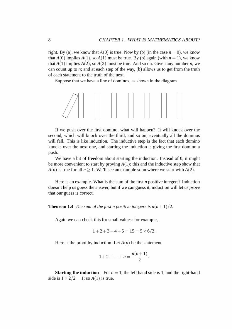
Suppose that we have a line of dominos, as shown in the diagram.
������
������
HH
HH
If we push over the first domino, what will happen? It will knock over thesecond, which will knock over the third, and so on; eventually all the dominoswill fall. This is like induction. The inductive step is the fact that each dominoknocks over the next one, and starting the induction is giving the first domino apush.
We have a bit of freedom about starting the induction. Instead of 0, it mightbe more convenient to start by provingA(1); this and the inductive step show thatA(n) is true for alln≥ 1. We’ll see an example soon where we start withA(2).
Here is an example. What is the sum of the firstn positive integers? Inductiondoesn’t help usguessthe answer, but if we can guess it, induction will let usprovethat our guess is correct.
Theorem 1.4 The sum of the first n positive integers is n(n+1)/2.
Again we can check this for small values: for example,
1+2+3+4+5 = 15= 5×6/2.
Here is the proof by induction. LetA(n) be the statement
1+2+ · · ·+n =n(n+1)
2.
Starting the induction Forn = 1, the left hand side is 1, and the right-handside is 1×2/2 = 1; soA(1) is true.

1.3. PROOF BY INDUCTION 9
The inductive step Suppose thatA(n) is true; that is,
1+2+ · · ·+n =n(n+1)
2.
We have to prove thatA(n+1) is true.Now the left-hand side ofA(n+ 1) is 1+ 2+ · · ·+ n+(n+ 1). Since we are
assuming thatA(n) is true, this is equal to
n(n+1)2
+(n+1) =n(n+1)
2+
2(n+1)2
=(n+1)(n+2)
2,
after a little bit of algebraic manipulation. But this is exactly the right-hand sideof A(n+1); it is what we get from the expressionn(n+1)/2 if we substituten+1in place ofn. So the left and right sides ofA(n+1) are equal, andA(n+1) is true.
By induction, we have proved thatA(n) is true for alln≥ 1.
Unfinished business I told you earlier that if a natural numbern is greater than 1and is not prime, then it is divisible by some prime number less thann. In otherwords,
Theorem 1.5 Every natural number n> 1 has a prime factor.
We prove this theorem by induction. TakeA(n) to be the statement “everynatural numberk satisfying 1< k ≤ n has a prime factor”. We proveA(n) byinduction.
Starting the induction We can conveniently start the induction withn = 2:there is only one numberk satisfying 1< k≤ 2, namelyk = 2, and it has a primefactor, namely 2. [Note: We could start the induction withn = 1: there are nonumbersk satisfying 1< k≤ 1, and so any statement at all is true for all of them!But you may feel uncomfortable with this sort of argument!]
The inductive step We assume thatA(n) is true, and we have to proveA(n+1). In other words, we assume that every natural numberk satisfying 1< k≤ nhas a prime factor, and we have to prove that every natural numberk satisfying1 < k ≤ n+ 1 has a prime factor. Well, we don’t have to prove it forall thesenumbers, since the hypothesisA(n) shows that it is true fork = 2,3, . . . ,n; weonly have to prove it fork = n+1.
Case 1:n+1 is prime. If it is prime, it certainly has a prime factor, namely itself.

10 CHAPTER 1. WHAT IS MATHEMATICS ABOUT?
Case 2:n+ 1 is not prime; son+ 1 = ab for some natural numbersa andb,where neither factor is 1. Then each factor must be smaller thann+1. So,for example, 1< a≤ n. By A(n), we know thata has a prime factorp. Thenp is also a factor ofn+1, and we have finished.
This completes the proof by induction.
Here is a variant on the principle of induction. Sometimes you might find thiseasier to apply.
Suppose that we are trying to prove a statementA(n). We begin by arguing bycontradiction: we assume thatA(n) isn’t true for all values ofn, that is, there issome value ofn for which it is false. So there must be a smallest value ofn forwhichA(n) is false. Now thisn has the property thatA(n) is false butA(m) is truefor all numbersm smaller thann – so we calln the “minimal counterexample” tothe statement we are trying to prove. (Some people calln the “least criminal”.) Ifwe can show that no minimal counterexample can exist, then we have proved thatA(n) is true for alln.
Why is this the same as induction? Well, letn be the minimal counterexample,and remember we are trying to get a contradiction. Mayben = 0. To show acontradiction, we have to show thatA(0) is true. Or mayben > 0. Now A(n)is false andA(n−1) is true, so if we could show thatA(n−1) impliesA(n), wewould have a contradiction in this case too. So the two things we have to prove areprecisely the same as starting the induction and doing the inductive step in a proofby induction. But sometimes it is easier to think about a minimal counterexample.
Take an induction proof and try writing it out in the “minimal counterexample”style, and see which you prefer.
1.4 Some more mathematical terms
There are many other specialised terms in mathematics.
Theorem, Proposition, Lemma, Corollary These words all mean the samething: a statement which we can prove. We use them for slightly different pur-poses.
A theoremis an important statement which we can prove. Apropositionisa statement which is less important. (Of the five theorems we’ve seen so far, Iwould normally call two of them “theorems” and the other three “propositions”;can you guess which are which?) Acorollary is a statement which follows easilyfrom a theorem or proposition. For example, the statement
Let n be a natural number. Then n2 is odd if and only if n is odd.

1.4. SOME MORE MATHEMATICAL TERMS 11
follows easily from Theorem 1 in the notes, so I could call it a corollary of Theo-rem 1. Finally, alemmais a statement which is proved as a stepping stone to somemore important theorem. So I could have called Theorem 1 a lemma for the proofof Theorem 2. (Remember how we used Theorem 1 in the proof of Theorem 2.)
Of course these words are not used very precisely; it is a matter of judgmentwhether something is a theorem, proposition, or whatever. For example, there is avery famous theorem calledFermat’s Last Theorem, which is the following:
Theorem 1.6 Let n be a natural number bigger than2. Then there are no positiveintegers x,y,z satisfying xn +yn = zn.
This was proved fairly recently by Andrew Wiles, so why do we attribute it toFermat?
Pierre de Fermat wrote thestatement of this theorem in themargin of one of his books. Hesaid, “I have a truly wonderfulproof of this theorem, but thismargin is too small to contain it.”No such proof was ever found, andtoday we don’t believe he had aproof; but the name stuck.
Conjecture The proof of Fermat’s Last Theorem is rather complicated, and Iwill not give it here! Note that, for about 350 years (between Fermat and Wiles),“Fermat’s Last Theorem” wasn’t a theorem, since we didn’t have a proof! Astatement that we think is true but we can’t prove is called aconjecture. So weshould really have called itFermat’s Conjecture.
An example of a conjecture which hasn’t yet been proved isGoldbach’s con-jecture:
Every even number greater than 2 is the sum of two prime numbers.
To prove this is probably very difficult. But to disprove it, a single counterex-ample (an even number which is not the sum of two primes) would do.
Prove, show, demonstrate These words all mean the same thing. We havediscussed how to give a mathematical proof of a statement. These words all askyou to do that.

12 CHAPTER 1. WHAT IS MATHEMATICS ABOUT?
Converse The converse of the statement “A impliesB” (or “if A thenB”) is thestatement “B impliesA”. They are not logically equivalent, as we saw when wediscussed “if” and “only if”. You should regard the following conversation as awarning! Alice is at the Mad Hatter’s Tea Party and the Hatter has just asked hera riddle: ‘Why is a raven like a writing-desk?’
‘Come, we shall have some fun now!’ thought Alice. ‘I’m glad they’vebegun asking riddles.–I believe I can guess that,’ she added aloud.
‘Do you mean that you think you can find out the answer to it?’ said theMarch Hare.
‘Exactly so,’ said Alice.‘Then you should say what you mean,’ the March Hare went on.‘I do,’ Alice hastily replied; ‘at least–at least I mean what I say–that’s
the same thing, you know.’‘Not the same thing a bit!’ said the Hatter. ‘You might just as well
say that “I see what I eat” is the same thing as “I eat what I see”!’ ‘Youmight just as well say,’ added the March Hare, ‘that “I like what I get” is thesame thing as “I get what I like”!’ ‘You might just as well say,’ added theDormouse, who seemed to be talking in his sleep, ‘that “I breathe when Isleep” is the same thing as “I sleep when I breathe”!’
‘It is the same thing with you,’ said the Hatter, and here the conversationdropped, and the party sat silent for a minute, while Alice thought over allshe could remember about ravens and writing-desks, which wasn’t much.
Definition To take another example from Lewis Carroll, recall Humpty Dumpty’sstatement: “When I use a word, it means exactly what I want it to mean, neithermore nor less”.
In mathematics, we use a lot of words with very precise meanings, often quitedifferent from their usual meanings. When we introduce a word which is to havea special meaning, we have to say precisely what that meaning is to be. Usually,the word being defined is written in italics. For example, in Geometry I, you metthe definition
An m× n matrix is an array of numbers set out inm rows andncolumns.
From that point, whenever the lecturer uses the word “matrix”, it has this meaning,and has no relation to the meanings of the word in geology, in medicine, and inscience fiction.
If you are trying to solve a coursework question containing a word whosemeaning you are not sure of, check your notes to see if you can find a definitionof that word.

1.4. SOME MORE MATHEMATICAL TERMS 13
Exercises
1.1 Write down and prove the contrapositive of the statement
If x is an irrational number then 1−x is an irrational number.
1.2 Find counterexamples to the statements
(a) Every odd number is prime.
(b) Every prime number is odd.
1.3 Prove by induction that
12 +22 + · · ·+n2 =n(n+1)(2n+1)
6.
1.4 Let n be a positive natural number, and suppose thatn has the property thatevery positive natural number smaller thann/2 dividesn. Prove thatn≤ 6, andhence find all numbersn with this property.
1.5 Define thebinomial coefficient
(nk
)for natural numbersn andk by the rule
(nk
)=
n· (n−1) · · ·(n−k+1)k · (k−1) · · ·1
=
{n!
k! (n−k)!if 0 ≤ k≤ n,
0 if k > n.
(Heren! is the product of the natural numbers from 1 ton.)
(a) I have given you two definitions here. Prove that they are equivalent.
(b) Prove that (nk
)+
(n
k−1
)=
(n+1
k
).
(c) Using this and induction onn, prove theBinomial Theorem:
(a+b)n =n
∑k=0
(nk
)akbn−k
for positive integersn.
1.6 Prove thatn
∑i=0
(ik
)=
(n+1k+1
).
14 CHAPTER 1. WHAT IS MATHEMATICS ABOUT?
1.7 Find the mistake in the following proof of the “Theorem”:All triangles areisosceles. (You will need to draw a figure!)
Proof Given any triangleABC, let D be the point inside the triangle where thebisector of the angleA meets the perpendicular bisector of the sideBC. Now letDM be the perpendicular fromD to AB andDN be the perpendicular fromD toAC.
Step 1 The trianglesADN andADM are congruent (since they have the sameangles and they also have the sideAD in common).
Step 2 The trianglesCDN andBDM are congruent (sinceDN = DM fromStep 1, andDC = DB asDL is the perpendicular bisector ofBC by construction,and the anglesCND andBMD are both right angles).
Step 3 From Step 1 we haveAN= AM, and from Step 2 we haveNC= MB.HenceAC= AB.
Chapter 2
Numbers
Algebra begins by considering numbers and their properties, and moves on toother kinds of mathematical objects. In this section of the notes, we will look atnumbers.
The important sets of numbers are:
• the natural numbers, denoted byN;
• the integers, denoted byZ;
• the rational numbers, denoted byQ;
• the real numbers, denoted byR;
• the complex numbers, denoted byC.
The notation we use for them is a special typeface called “blackboard bold”. Orig-inally, number systems were printed in bold type:N,Z, etc.; lecturers writing onthe blackboard couldn’t write in bold, so invented a different way of doing it; thenthe printers had to catch up by designing a typeface.
The notationN, R andC for natural, real and complex numbers is easy toremember; but what about the others? If the real numbers are calledR, then weneed a different letter for the rational numbers; we chooseQ for “quotients”, sinceevery rational number has the forma/b wherea andb are integers. TheZ comesfrom the German wordZahlen, meaning numbers.
In this section, you will not learndefinitionsof numbers. I will assume thatyou know what numbers are; we will revise some of their properties.
15
16 CHAPTER 2. NUMBERS
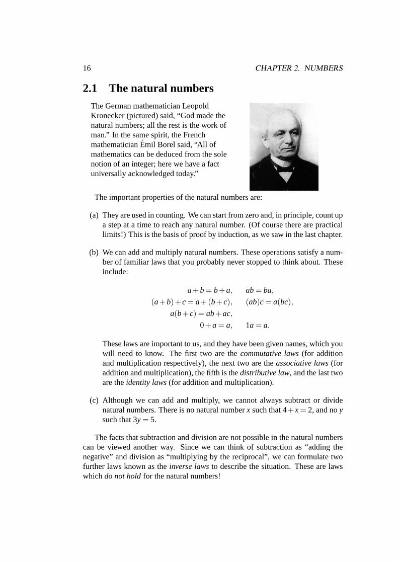
2.1 The natural numbersThe German mathematician LeopoldKronecker (pictured) said, “God made thenatural numbers; all the rest is the work ofman.” In the same spirit, the FrenchmathematicianEmil Borel said, “All ofmathematics can be deduced from the solenotion of an integer; here we have a factuniversally acknowledged today.”
The important properties of the natural numbers are:
(a) They are used in counting. We can start from zero and, in principle, count upa step at a time to reach any natural number. (Of course there are practicallimits!) This is the basis of proof by induction, as we saw in the last chapter.
(b) We can add and multiply natural numbers. These operations satisfy a num-ber of familiar laws that you probably never stopped to think about. Theseinclude:
a+b = b+a, ab= ba,
(a+b)+c = a+(b+c), (ab)c = a(bc),a(b+c) = ab+ac,
0+a = a, 1a = a.
These laws are important to us, and they have been given names, which youwill need to know. The first two are thecommutative laws(for additionand multiplication respectively), the next two are theassociative laws(foraddition and multiplication), the fifth is thedistributive law, and the last twoare theidentity laws(for addition and multiplication).
(c) Although we can add and multiply, we cannot always subtract or dividenatural numbers. There is no natural numberx such that 4+x = 2, and noysuch that 3y = 5.
The facts that subtraction and division are not possible in the natural numberscan be viewed another way. Since we can think of subtraction as “adding thenegative” and division as “multiplying by the reciprocal”, we can formulate twofurther laws known as theinverse lawsto describe the situation. These are lawswhichdo not holdfor the natural numbers!

2.2. THE INTEGERS 17
Additive inverse law: For any elementa, there exists an element−a such thata+(−a) = 0.
Multiplicative inverse law: For any elementa 6= 0, there exists an elementa−1
such thata·a−1 = 1.
Notice the exclusion in the multiplicative inverse law; we can’t divide by zero!
The laws for the natural numbers can be interpreted in terms of counting. Thisdepends on two obvious principles:
• a row ofa dots, followed by a row ofb dots, containsa+b dots.
• a rectangle of dots with sidesa andb containsabdots.
The figure illustrates this fora = 2 andb = 3.
s s s s s2+3 = 5
s s ss s s3×2 = 6
Now the laws of algebra can be explained by geometric transformations. Forexample, the picture below shows the commutative law for addition and the dis-tributive law. In the first case, we have reflected the figure left-to-right.
s s s s s s s s s s3+2 = 2+3
s s s s s s ss s s s s s s(3+4)×2 = 3×2+4×2
You are invited to produce similar geometric explanations of the commutative lawfor multiplication and the associative laws.
2.2 The integers
We enlarge the number system because we are trying to solve equations whichcan’t be solved in the original system. At every stage in the process, people first

18 CHAPTER 2. NUMBERS
thought that the new numbers were just aids to calculating, and not “proper” num-bers. The names given to them reflect this: negative numbers, improper fractions,irrational numbers, imaginary numbers! Only later were they fully accepted. Youmay like to read the bookImagining Numbersby Barry Mazur, about the longprocess of accepting imaginary numbers.
Anyway, we can’t always subtract natural numbers, so we add negative num-bers to make it possible. Theintegersare the natural numbers together with theirnegatives. So addition, subtraction, and multiplication are all possible for inte-gers. The laws we met for natural numbers all continue to hold for integers. Also,the additive inverse law (but not the multiplicative inverse law) holds for integers.
The natural numbers 1,2, . . . are positive, while−1,−2, . . . are negative. In-tegers satisfy the law of signs: the product of a positive and a negative number isnegative, while the product of two negative numbers is positive.
2.3 The rational numbers
In a similar way, rational numbers are introduced because we cannot always divideintegers. A rational number is a number which can be written as a fraction
ab
wherea andb are integers andb 6= 0. We require that multiplying or dividing nu-merator and denominator (top and bottom) of a fraction by the same thing doesn’tchange the fraction. So, if the denominator is negative, we can multiply by−1to make it positive; and if numerator and denominator have a common factor, wecan divide by it. (We say that a fractiona/b is in its lowest termsif the highestcommon factor ofa andb is 1.)
We can write rules for adding and multiplying rational numbers:
ab
+cd
=ad+bc
bd,
ab− c
d=
ad−bcbd
,
ab× c
d=
acbd
,ab÷ c
d=
adbc
if c 6= 0.
The last rule says: to divide by a fraction, turn it upside down and multiply.So, for rational numbers, addition, subtraction, multiplication, and division
(except by 0) are all possible. The rules we met for natural numbers all hold forrational numbers, and so do the two inverse laws.

2.4. THE REAL NUMBERS 19
2.4 The real numbers
There are still many equations we can’t solve with rational numbers. One suchequation isx2 = 2. (we saw Pythagoras’ proof of this in the last chapter.) Otherequations involve functions from trigonometry (such as sinx= 1, which has the ir-rational solutionx= π/2) and calculus (such as logx= 1, which has the irrationalsolutionx = e).
So, we take a larger number system in which these equations can be solved,thereal numbers. A real number is a number that can be represented as an infinitedecimal. This includes all the rational numbers and many more, including thesolutions of the three equations above; for example,
25 = 0.417 = 0.142857142857. . . ,
√2 = 1.41421356237. . . ,π
2 = 1.57079632679. . . ,
e = 2.71828182846. . .
In the last three cases, we cannot write out the number exactly as a decimal, butwe assume that the approximation gets better as the number of digits increases.
We can add, subtract, multiply, and divide (except by zero) in the system ofreal numbers, and the laws we met earlier (including the inverse laws) all holdhere too.
2.5 The complex numbers
The final extension arises because there are still equations we can’t solve, such asx2 = −1 (which has no real solution) orx3 = 2 (which has only one, though forvarious reasons we would like it to have three). It turns out that the first equationis the crucial one.
A complex numberis a number of the forma+ bi, wherea and b are realnumbers, and i is a mysterious symbol which will have the property that i2 =−1.The rules for addition and multplication are
(a+bi)+(c+di) = (a+c)+(b+d)i,(a+bi)(c+di) = (ac−bd)+(ad+bc)i.
You can work out the rule for subtraction. How do we divide? You can check thatthe rule above gives
(a+bi)(a−bi) = a2 +b2,

20 CHAPTER 2. NUMBERS
which is a positive number unlessa = b = 0. So, to divide bya+bi, we multiplyby (
aa2 +b2
)−
(b
a2 +b2
)i.
Thus, in the complex numbers, we can add, subtract, multiply, and divide(except by zero), and the laws we met earlier (including the inverse laws) all applyhere too.
Complex numbers are not called complex because they are complicated: amodern advertising executive would certainly have come up with a different name!They are called “complex” because each complex number is built of two parts,each of which is simpler (being a real number).
Here, unlike for the other forms of numbers, we don’t have to take on trustthat the laws hold; we can prove them. Here, for example, is the distributive law.Let z1 = a1 +b1i, z2 = a2 +b2i, andz3 = a3 +b3i. Now
z1(z2 +z3) = (a1 +b1i)((a2 +a3)+(b2 +b3)i)= (a1(a2 +a3)−b1(b2 +b3))+a1(b2 +b3)+b1(a2 +a3))i,
and
z1z2 +z1z3 = ((a1a2−b1b2)+(a1b2 +a2b1)i)+((a1a3−b1b3)+(a1b3 +a3b1)i)= (a1a2−b1b2 +a1a3−b1b3)+(a1b2 +a2b1 +a1b3 +a3b1)i,
and a little bit of rearranging shows that the two expressions are the same.
If z= a+bi is a complex number (wherea andb are real), we say thata andbare thereal partandimaginary partof z respectively. The complex numbera−biis called thecomplex conjugateof z, and is written asz. So the rules for additionand subtraction can be put like this:
To add or subtract complex numbers, we add or subtract their realparts and their imaginary parts.
The rule for multiplication looks more complicated as we have written it out.There is another representation of complex numbers which makes it look simpler.Let z= a+bi. We define themodulusandargumentof z by
|z| =√
a2 +b2,
arg(z) = θ where cosθ = a/|z| and sinθ = b/|z|.
In other words, if|z|= r and arg(z) = θ , then
z= r(cosθ + i sinθ).
Now the rules for multiplication and division are:

2.6. THE COMPLEX PLANE, OR ARGAND DIAGRAM 21
To multiply two complex numbers, multiply their moduli and addtheir arguments. To divide two complex numbers, divide their moduliand subtract their arguments.
2.6 The complex plane, or Argand diagram
The complex numbers can be represented geometrically, by points in the Eu-clidean plane (which is usually referred to as theArgand diagramor thecomplexplanefor this purpose. The complex numberz= a+bi is represented as the pointwith coordinates(a,b). Then|z| is the length of the line from the origin to thepointz, and arg(z) is the angle between this line and thex-axis. See Figure 2.1.
��
��
��
��
��
��
r
r z= a+bi
|z|= r
a = r cosθ
b = r sinθ
θ
0
Figure 2.1: The Argand diagram
In terms of the complex plane, we can give a geometric description of additionand multiplication of complex numbers. The addition rule is the same as youlearned for adding vectors in Geometry I, namely, theparallelogram rule(seeFigure 2.2).
Multiplication is a little bit more complicated. Letz be a complex numberwith modulusr and argumentθ , so thatz = r(cosθ + i sinθ). Then the wayto multiply an arbitrary complex number byz is a combination of a stretch and arotation: first we expand the plane so that the distance of each point from the originis multiplied byr; then we rotate the plane through an angleθ . See Figure 2.3,where we are multiplying by 1+ i =
√2(cos(π/4)+ i sin(π/4)); the dots represent
the stretching out by a factor of√
2, and the circular arc represents the rotation byπ/4.
Now let’s check the correctness of our rule for multiplying complex numbers.Remember that the rule is: to multiply two complex numbers, we multiply themoduli and add the arguments. To see that this is correct, suppose thatz1 and

22 CHAPTER 2. NUMBERS
r
rr
r
������
������
�����
�������
������
����*
�����
�����*
�
�
�
�
0
z1
z2
z1 +z2
Figure 2.2: Addition of complex numbers
r���
��
��
��...
......r
���������������r
.
..................................
.................................
................................
.................................
..................................
...................................
...................................
...................................
........................................................................
0
3+2i
(3+2i)(1+ i)= 1+5i
Figure 2.3: Multiplication of complex numbers
z2 are two complex numbers; let their moduli ber1 andr2, and their argumentsθ1 +θ2. Then
z1 = r1(cosθ1 + i sinθ1),z2 = r2(cosθ2 + i sinθ2).
Then
z1z2 = r1r2(cosθ1 + i sinθ1)(cosθ2 + i sinθ2)= r1r2((cosθ1cosθ2−sinθ1sinθ2)+(cosθ1sinθ2 +sinθ1cosθ2)i)= r1r2(cos(θ1 +θ2)+ i sin(θ1 +θ2)),
which is what we wanted to show.

2.6. THE COMPLEX PLANE, OR ARGAND DIAGRAM 23
From this we can proveDe Moivre’s Theorem:
Theorem 2.1 For any natural number n, we have
(cosθ + i sinθ)n = cosnθ + i sinnθ .
Proof The proof is by induction. Starting the induction is easy since(cosθ +i sinθ)0 = 1 and cos0+ i sin0= 1.
For the inductive step, suppose that the result is true forn, that is,
(cosθ + i sinθ)n = cosnθ + i sinnθ .
Then
(cosθ + i sinθ)n+1 = (cosθ + i sinθ)n · (cosθ + i sinθ)= (cosnθ + i sinnθ)(cosθ + i sinθ)= cos(n+1)θ + i sin(n+1)θ ,
which is the result forn+1. So the proof by induction is complete.Note that, in the second line of the chain of equations, we have used the in-
ductive hypothesis, and in the third line, we have used the rule for multiplyingcomplex numbers.
The argument is clear if we express it geometrically. To multiply by the com-plex number(cosθ + i sinθ)n, we rotaten times through an angleθ , which is thesame as rotating through an anglenθ .
De Moivre’s Theorem is useful in deriving trigonometrical formulae. For ex-ample,
cos3θ + i sin3θ = (cosθ + i sinθ)3
= (cos3θ −3cosθ sin2θ)+(3cos2θ sinθ −sin3
θ)i,
so
cos3θ = cos3θ −3cosθ sin2θ ,
sin3θ = 3cos2θ sinθ −sin3θ .
These can be converted into the more familiar forms cos3θ = 4cos3θ −3cosθand sin3θ = 3sinθ −4sin3
θ by using the equation cos2θ +sin2θ = 1.

24 CHAPTER 2. NUMBERS
Exercises
2.1 Prove by induction or otherwise that
11·2
+1
2·3+ · · ·+ 1
(n−1) ·n=
n−1n
.
2.2 Use De Moivre’s Theorem to express cos4x as a polynomial in cosx, and toexpress sin4x as a polynomial in sinx.
2.3 Find √2+
√2+
√2+ · · ·.
2.4 Thequaternionsform a number system discovered by Hamilton. They havethe forma+ bi + cj + dk, wherea,b,c,d ∈ R and i, j, k are new symbols whichsatisfy
i2 = j2 = k2 = ijk =−1.
(a) Write down rules for the sum and product of two quaternions.
(b) Show that the associative law for multiplication holds for quaternions.
(c) Show that(a+ bi + cj + dk)(a− bi − cj − dk) = (a2 + b2 + c2 + d2), andhence show that the quaternions satisfy the inverse law for multiplication(that is, every non-zero quaternion has a multiplicative inverse).

Chapter 3
Other algebraic systems
In this section, we will look at other algebraic systems which have operationswhich resemble addition and multiplication for number systems. These operationssatisfy some of the laws which hold for numbers, but not necessarily all of them.A reminder: we are interested in the following laws:
Commutative laws:a+b = b+a, ab= ba
Associative laws:(a+b)+c = a+(b+c), (ab)c = a(bc)
Distributive law:a(b+c) = ab+ac
Identity laws: 0+a = a, 1a = a
Inverse laws: For alla there exists(−a) such thata+(−a) = 0; for all a 6= 0,there existsa−1 such thata·a−1 = 1.
We have to be a bit careful about what the identity laws mean, since in other alge-braic systems there will not be numbers 0 and 1 to use here. The identity law formultiplication should mean that there is a particular elemente (say) in our systemsuch thatea= a for every elementa. In the case of number systems, the number1 has this property. Similarly we have to be careful about the interpretation of−aanda−1 in the inverse laws. But notice that we don’t even have to try to check theadditive or multiplicative inverse laws unless the additive or multiplicative identitylaws hold.
3.1 Vectors
In Geometry I, you learned how to add 3-dimensional vectors, and two differentways to multiply them: the scalar product or dot product, and the vector product
25

26 CHAPTER 3. OTHER ALGEBRAIC SYSTEMS
or cross product. Given two vectorsu,v, we denote their sum byu+v, their dotproduct byu ·v, and their cross product byu×v.
(We can’t do something likeu in handwriting, or writing on the blackboard.So you should write the vectoru asu, as you did in the Geometry I course.)
Remember that we can represent a vector by a column consisting of threenumbers; for example,
u = 2i + j −5k =
2−15
.
Addition The commutative and associative laws hold for vector addition; so
does the zero and inverse laws, if we take the vector0 =
000
to be the zero
element:
u+v = v+u,
(u+v)+w = u+(v+w),0+v = v,
v+(−v) = 0.
These can all be proved by a calculation. For example, here is a proof of theassociative law. Let
u =
abc
, v =
pqr
, w =
xyz
.
Then
(u+v)+w =
a+ pb+qc+ r
+
xyz
=
(a+ p)+x(b+q)+y(c+ r)+z
,
u+(v+w) =
abc
+
p+xq+yr +z
=
a+(p+x)b+(q+y)c+(r +z)
,
and(a+ p)+x = a+(p+x), etc., since the associative law holds for addition ofreal numbers. So the two expressions are equal.
Notice what we have done here: we used the associative law for the real num-bers to prove it for 3-dimensional vectors.

3.1. VECTORS 27
Scalar product Asking about the associative law or other laws for the scalarproduct doesn’t really make sense, since the scalar product of two vectors is anumber, not a vector! So(u ·v) ·w is meaningless.
The lesson is that the operations we will be studying must take two objects ofsome kind and combine them into another object of the same kind.
Vector product Remember the formula for the vector product:abc
×
xyz
=
∣∣∣∣∣∣i a xj b yk c z
∣∣∣∣∣∣ ,or, to put it another way,
(ai +bj +ck)× (xi +yj +zk) = (bz−cy)i +(cx−az)j +(ay−bx)k.
(This was not thedefinition, but it was proved in Part 5 of the notes that thisformula holds.)
What properties does it have? You also met these properties in the Geometry Icourse.
Associative law: This does not hold. Remember thatv×v = 0 for any vectorv.Now
(i× i)× j = 0× j = 0,
i× (i× j) = i×k =−j .
(Remember that todisprovesomething like the associative law, a singlecounterexample is enough!)
Commutative law: This does not hold either. In fact, I hope you remember fromGeometry I that
u×v =−(v×u)
for any two vectorsu andv. To get a specific counterexample, we couldobserve that
i× j = k, j × i =−k.
Distributive law: This one is true:
u× (v+w) = (u×v)+(u×w).
How do you prove this?

28 CHAPTER 3. OTHER ALGEBRAIC SYSTEMS
Identity law: This one also fails. There cannot be a vectore with the propertythat e× v = v for any choice ofv, becausee× v is always perpendicularto v!
The lesson here is that even nice operations might fail to satisfy the usual lawsfor numbers.
3.2 Matrices
Matrices form another class of objects which can be added and multiplied. Wewill consider just 2×2 matrices, as these illustrate the general principles. Recall
the rules, that you learned in Geometry I. LetA =(
a bc d
)andB =
(e fg h
)be
two matrices. We will take the entriesa, . . . ,h to be arbitrary real numbers.
Addition The sum of two matricesA andB is the matrix obtained by addingcorresponding elements ofA andB:(
a bc d
)+
(e fg h
)=
(a+e b+ fc+g d+h
).
Multiplication The rule for multiplication is more complicated:(a bc d
)(e fg h
)=
(ae+bg a f+bhce+dg c f+dh
).
It works like this. To work out the entry in the first row and second column of theproductAB, we take the first row ofA (which is(a b)), and the second column
of B (which is
(fh
); multiply corresponding elements (a by f , andb by h), and
add the products, to geta f +bh. The rule for the other entries inAB is similar.Do these operations satisfy the laws we wrote down earlier?
Addition The commutative, associative, identity, and inverse laws all hold.To verify thatA+ B = B+ A, we have to show that corresponding entries of
these matrices are equal. These entries are obtained by adding correspondingentries inA andB in either order; the results are equal. In detail,(
a bc d
)+
(e fg h
)=
(a+e b+ fc+g d+h
),(
e fg h
)+
(a bc d
)=
(e+a f +bg+c h+d
),

3.2. MATRICES 29
and the matrices on the right are equal becausea+e= e+a etc.The associative law is true, and the argument to prove it is similar. If we define
thezero matrixto be
O2×2 =(
0 00 0
),
then we haveO2×2 +A = A for any matrixA; for, to work outO2×2 +A, we addzero to each entry ofA, which doesn’t change it. Similarly, for any matrixA,we let−A be the matrix whose entries are the negatives of the entries ofA; thenA+(−A) = O.
Multiplication Here we find our first surprise: The commutative law for multi-plication fails! Remember that to disprove a general assertion, we only need onecounterexample:(
1 23 4
)(5 67 8
)=
(19 2243 50
)6=
(23 3431 46
)=
(5 67 8
)(1 23 4
).
[How did I find this example? Trial and error; I wrote down the first two matricesI could think of, multiplied them both ways round, and found that the results weredifferent.]
Despite this, the associative law and the identity law do both hold for matrixmultiplication. For the associative law, there is no alternative but to multiply it outand see:(
a bc d
)((e fg h
)(i jk l
))=
(a bc d
)(ei+ f k e j+ f lgi+hk g j+hl
)=
(a(ei+ f k)+b(gi+hk) . . .
. . . . . .
),((
a bc d
)(e fg h
))(i jk l
)=
(ae+bg a f+bhce+dg c f+dh
)(i jk l
)=
((ae+bg)i +(a f +bh)k . . .
. . . . . .
).
Algebraic manipulation shows that
a(ei+ f k)+b(gi+hk) = (ae+bg)i +(ce+dg)k.
[Take a look at this manipulation. We first expand the brackets on the left, usingthe distributive law. This givesa(ei)+a( f k)+b(gi)+b(hk). Now use the associa-tive law for multiplication to switch this into(ae)i +(a f)k+(bg)i +(bh)k. Thenthe commutative law for addition changes this to(ae)i +(bg)i +(a f)k+(bh)k,

30 CHAPTER 3. OTHER ALGEBRAIC SYSTEMS
and the distributive law once more turns this into the right-hand expression. Oh,and I forgot to mention that I used the associative law for addition without tellingyou, when I wrote down the sum of four terms without telling you where thebrackets go! So almost all the laws for real numbers get used.]
To prove the identity law for multiplication, we have to know what the identitymatrix is. Since the zero matrix has every entry zero, you might guess that theidentity matrix has every entry 1, but it doesn’t:(
1 11 1
)(1 23 4
)=
(4 64 6
).
In fact the identity matrix has ones on the main diagonal and zeros elsewhere:
I2 =(
1 00 1
).
We haveI2A = A for any 2×2 matrixA:(1 00 1
)(a bc d
)=
(a bc d
).
Now another possible problem might occur to you. Since multiplication is notcommutative, is it true thatAI2 = A for anyA? Well, yes it is:(
a bc d
)(1 00 1
)=
(a bc d
),
as you can check. [You may also notice that, as well as the identity law for mul-tiplication, we use the fact that 0a = 0 for any real numbera and the zero law foraddition.]
The inverse law for multiplication does not hold. For example, ifA=(
1 00 0
),
then there is no matrixB such thatAB= I2. You learned in Geometry I that thecondition for a matrix to have an inverse is that itsdeterminantis not zero.
Distributive law: I leave it to you to check that
A(B+C) = AB+AC
for any matricesA,B,C. You might even want to check which laws for real num-bers are used in the proof. Because multiplication is not commutative, we can alsocheck the other way round:
(B+C)A = BA+CA

3.3. POLYNOMIALS 31
for any matricesA,B,C.
We use the notationM2×2(R) for the set of all 2×2 matrices with real numbersas entries. (We call these matrices “real matrices” for short.) As you can see, wecan easily generalise this notation. By changing the subscript, we can talk aboutthe set of matrices of different size, say 3×3; and by puttingZ, Q or C in placeof R, we can talk about matrices whose entries are integers, rational numbers, orcomplex numbers.
3.3 Polynomials
You can think of a polynomial as a function which can be written as a sum ofterms, each of which is a power ofx multiplied by a constant. So “the polynomialx2” should really be “the polynomial 1x2”. We write x1 asx, and leave outx0
altogether (just writing the constant). If the coefficient of a power ofx is zero, weusually don’t bother writing it: so we write 2x2 + 3 rather than 2x2 + 0x+ 3. Ofcourse, if all the terms are zero, we have to write something; so we just write 0.
So a typical polynomial has the form
anxn +an−1xn−1 + · · ·+a1x+a0.
Note that a constanta0 is a special kind of polynomial called aconstant polyno-mial.
Thedegreeof a polynomial is the largest numbern such that the polynomialcontains a termanxn with an 6= 0. Thus, a non-zero constant polynomial has de-gree 0, since it has the forma0x0. The zero polynomial 0 doesn’t have a degree,since it doesn’t have any non-zero terms! [Be warned: some people say that ithas degree−1; others say that it has degree−∞. Of course, these are merelyconventions.]
Addition and multiplication You already know how to add and multiply poly-nomials. But it is difficult to give a proper mathematical definition. For example,(
2x2 +3)+
(x3 +x−5
)= x3 +2x2 +x−2.
We can’t just say “add corresponding terms”, since some terms may be missing;we have first to put the missing terms in with coefficients 0. For multiplication, wemultiply each term of the first factor by each term of the second, and then gatherup terms involving the same power ofx:(
2x2 +3)(
x3 +x−5)
= 2x5 +(2x3 +3x3)−10x2 +3x−15
= 2x5 +5x3−10x2 +3x−15.

32 CHAPTER 3. OTHER ALGEBRAIC SYSTEMS
I ask you to take on trust for now that it is possible to give good definitions ofaddition and multiplication of polynomials, and to show that they do satisfy thecommutative, associative and identity laws for both addition and multiplication,the inverse law for addition, and the distributive law.
We use the notationR[x] for the set of all polynomials with real numbers ascoefficients. (We call them “real polynomials” for short.) As you can see, thisnotation can be generalised:Q[x] andC[x] denote the sets of polynomials withrational or complex numbers as coefficients. These sets satisfy the same rules foraddition and multiplication as the real polynomials.
3.4 Sets
Here is another example where we have an operation or rule of combination forobjects which are nothing like numbers.
Let S be a set. We regard it as a “universal set”; in Probability I, it was calledthesample space. Our objects will be subsets ofS .
Two operations which can be performed on sets are union and intersection,defined as follows:
Union: theunionof two setsA andB is the set of all elements lying in eitherAor B:
A∪B = {x : x∈ A or x∈ B}.We readA∪B as “A unionB”, or “A or B”.
Intersection: theintersectionof two setsA andB is the set of all elements lyingin bothA andB:
A∩B = {x : x∈ A andx∈ B}.We readA∩B as “A intersectionB”, or “A andB”.
We can represent sets byVenn diagrams, and show these two operations in adiagram as follows:
&%'$
&%'$
&%'$
&%'$
A∪B A∩B
A AB B
Here are some laws they satisfy.
Commutative laws A∪B = B∪A A∩B = B∩AAssociative laws A∪ (B∪C) = (A∪B)∪C A∩ (B∩C) = (A∩B)∩CIdentity laws A∪ /0 = A A∩S = A

3.4. SETS 33
When we come to the distributive law, there is a small surprise. To write downthe distributive law for numbers, we have to distinguish between addition andmultiplication. It is true that
a× (b+c) = (a×b)+(a×c),
but it isnot true that
a+(b×c) = (a+b)× (a+c).
For sets, which of our two operations should play the role of addition, and whichshould be multiplication?
It turns out that it works both ways round. We can replace “plus” by “or” and“times” by “and”, orvice versa:
Distributive laws A∩ (B∪C) = (A∩B)∪ (A∩C) A∪ (B∩C) = (A∪B)∩ (A∪C)
All of these assertions have similar proofs: draw a Venn diagram to convinceyourself, and then give a mathematical argument. Here is the proof of the firstdistributive law. I leave the Venn diagram to you.
x∈ A∩ (B∪C) ⇔ x∈ A andx∈ B∪C
⇔ (x∈ A andx∈ B) or (x∈ A andx∈C)⇔ x∈ (A∩B)∪ (A∩C).
So the two setsA∩ (B∪C) and(A∩B)∪ (A∩C) have the same members, andhence are equal.
The inverse laws are not true. For example, we saw that the zero element forthe operation of union is the empty set /0; and, given a setA which is not the emptyset, it is impossible to find a setB such thatA∪B = /0, sinceA∪B is at least aslarge asA. The failure of the inverse law for intersection is similar.
In Probability I, you saw several other operations on sets:difference, symmet-ric difference, andcomplement. You might like to check which of our laws aresatisfied by difference, or by symmetric difference, for example.
Exercises
3.1 (a) Find
(1 23 4
)(1 −13 −5
).
(b) Find the inverse of
(1 23 4
).

34 CHAPTER 3. OTHER ALGEBRAIC SYSTEMS
3.2 Find two matrices having entries 0 and 1 only which do not commute witheach other.
3.3 Show that the symmetric difference of sets satisfies the associative, commu-tative, identity and inverse laws, where the identity element is the empty set /0 andthe inverse of any setA is equal toA.
3.4 Recall the definition of the quaternions from the last chapter.
(a) Show that any quaternion can be formally written asa+v, wherea∈R andv is a 3-dimensional real vector.
(b) Show that
(a+v)+(b+w) = (a+b)+(v+w),(a+v)(b+w) = (ab−v ·w)+(aw+bv+v×w),
where· and× denote the dot and cross product of vectors.

Chapter 4
Relations and functions
4.1 Ordered pairs and Cartesian product
We write {x,y} to mean a set containing just the two elementsx andy. Moregenerally,{x1,x2, . . . ,xn} is a set containing just then elementsx1, x2, . . . ,xn.
The order in which elements come in a set is not important. So{y,x} is thesame set as{x,y}. This set is sometimes called anunordered pair.
Often, however, the order of the elements does matter, and we need a differentconstruction. We write theordered pairwith first elementx and second elementyas(x,y); this is not the same as(y,x) unlessx andy are equal. You have seen thisnotation used for the coordinates of points in the plane. The point with coordinates(2,3) is not the same as the point with coordinates(3,2). The rule for equality ofordered pairs is:
(x,y) = (u,v) if and only if x = u andy = v.
This notation can be extended to orderedn-tuples for largern. For example, apoint in three-dimensional space is given by anordered triple(x,y,z) of coordi-nates.
The idea of coordinatising the plane orthree-dimensional space by ordered pairs or triplesof real numbers was invented by Descartes. In hishonour, we call the system “Cartesian coordinates”.This great idea of Descartes allows us to usealgebraic methods to solve geometric problems, asyou saw in the Geometry I course last term.
By means of Cartesian coordinates, the set of all points in the plane is matchedup with the set of all ordered pairs(x,y), wherex andy are real numbers. We call
35

36 CHAPTER 4. RELATIONS AND FUNCTIONS
this setR×R, or R2. This notation works much more generally, as we nowexplain.
Let X andY be any two sets. We define theirCartesian product X×Y to bethe set of all ordered pairs(x,y), with x∈ X andy∈Y; that is, all ordered pairswhich can be made using an element ofX as first coordinate and an element ofYas second coordinate. We write this as follows:
X×Y = {(x,y) : x∈ X,y∈Y}.
You should read this formula exactly as in the explanation. The notation
{x : P}
means “the set of all elementsx for which P holds”. This is a very common wayof specifying a set.
If Y = X, we write X ×Y more briefly asX2. Similarly, if we have setsX1, . . . ,Xn, we letX1×·· ·×Xn be the set of all orderedn-tuples(x1, . . . ,xn) suchthatx1 ∈ X1, . . . ,xn ∈ Xn. If X1 = X2 = · · ·= Xn = X, say, we write this set asXn.
If the sets are finite, we can do some counting. Remember that we use thenotation|X| for the number of elements of the setX (not to be confused with|z|,the modulus of the complex numberz, for example).
Proposition 4.1 Let X and Y be sets with|X|= p and|Y|= q. Then
(a) |X×Y|= pq;
(b) |X|n = pn.
Proof (a) In how many ways can we choose an ordered pair(x,y) with x∈X andy ∈ Y? There arep choices forx, andq choices fory; each choice ofx can becombined with each choice fory, so we multiply the numbers.
(b) This is an exercise for you.
The “multiplicative principle” used in part (a) of the above proof is very im-portant. For example, ifX = {1,2} andY = {a,b,c}, then we can arrange theelements ofX×Y in a table with two rows and three columns as follows:
(1,a) (1,b) (1,c)(2,a) (2,b) (2,c)

4.2. RELATIONS 37
4.2 Relations
Suppose we are given a set of peopleP1, . . . ,Pn. What does the relation of beingsisters mean? For each ordered pair(Pi ,Pj), eitherPi andPj are sisters, or they arenot; so we can think of the relation as being a rule of some kind which answers“true” or “false” for each pair(Pi ,Pj). Mathematically, there is a more abstractway of saying the same thing; the relation of sisterhood is thesetof all orderedpairs(Pi ,Pj) for which the relation is true. (When I say thatPi andPj are sisters, Imean that each of them is the sister of the other.)
So we define arelation Ron a setX to be a subset of the Cartesian productX2 = X×X; that is, a set of ordered pairs. We think of the relation as holdingbetweenx andy if the pair(x,y) is in R, and not holding otherwise.
Here is another example. LetX = {1,2,3,4}, and letR be the relation “lessthan” (this means, the relation that holds betweenx andy if and only if x < y).Then we can writeRas a set by listing all the pairs for which this is true:
R= {(1,2),(1,3),(1,4),(2,3),(2,4),(3,4)}.
How many different relations are there on the setX = {1,2,3,4}? A relationon X is a subset ofX×X. There are 4×4 = 16 elements inX×X, by Proposi-tion 4.1. How many subsets does a set of size 16 have? For each element of theset, we can decide to include that element in the subset, or to leave it out. The twochoices can be made independently for each of the sixteen elements ofX2, so thenumber of subsets is
2×2×·· ·×2 = 216 = 65536.
So there are 65536 relations. Of course, not all of them have simple names like“less than”.
You will see that a relation like “less than” is writtenx < y; in other words,we put the symbol for the relation between the names of the two elements makingup the ordered pair. We could, if we wanted, invent a similar notation for anyrelation. Thus, ifR is a relation, we could writex R yto mean(x,y) ∈ R.
4.3 Equivalence relations and partitions
Just as there are certain laws that operations like multiplication may or may notsatisfy, so there are laws that relations may or may not satisfy. Here are someimportant ones.
Let Rbe a relation on a setX. We say thatR is
reflexiveif (x,x) ∈ R for all x∈ X;

38 CHAPTER 4. RELATIONS AND FUNCTIONS
symmetricif (x,y) ∈ R implies that(y,x) ∈ R;
transitiveif (x,y) ∈ Rand(y,z) ∈ R together imply that(x,z) ∈ R.
For example, the relation “less than” is not reflexive (since no element is lessthan itself); is not symmetric (sincex < y and y < x cannot both hold); but istransitive (sincex < y andy < zdo imply thatx < z). The relation of being sistersis not reflexive (it is debatable whether a girl can be her own sister, but a boycertainly cannot!), but it is symmetric. It is “almost” transitive: ifx andy aresisters, andy andz are sisters, thenx andz are sisters except in the case whenx = z. But this case can actually occur, so the relation is not transitive. (For it tobe transitive, the transitive law would have to hold without any exceptions.)
A very important class of relations are called equivalence relations. Anequiv-alence relationis a relation which is reflexive, symmetric, and transitive.
Before seeing the job that equivalence relations do in mathematics, we needanother definition.
Let X be a set. Apartition of X is a collection{A1,A2, . . .} of subsets ofXhaving the following properties:
(a) Ai 6= /0;
(b) Ai ∩A j = /0 for i 6= j;
(c) A1∪A2∪·· ·= X.
So each set is non-empty; no two sets have any element in common; and betweenthem they cover the whole ofX. The name arises because the setX is divided intodisjoint partsA1,A2, . . ..
A1 A2 A3 A4 A5
The statement and proof of the next theorem are quite long, but the messageis very simple: the job of an equivalence relation onX is to produce a partition ofX; every equivalence relation gives a partition, and every partition comes from anequivalence relation. This result is called theEquivalence Relation Theorem.
First we need one piece of notation. LetR be a relation on a setX. We writeR(x) for the set of elements ofX which are related toR; that is,
R(x) = {y∈ X : (x,y) ∈ R}.

4.3. EQUIVALENCE RELATIONS AND PARTITIONS 39
Theorem 4.2 (a) Let R be an equivalence relation on X. Then the sets R(x),for x∈ X, form a partition of X.
(b) Conversely, given any partition{A1,A2, . . .} of X, there is an equivalencerelation R on X such that the sets Ai are the same as the sets R(x) for x∈ X.
Proof (a) We have to show that the setsR(x) satisfy the conditions in the defini-tion of a partition ofX.
• For anyx, we have(x,x) ∈R (sinceR is reflexive), sox∈R(x); thusR(x) 6=/0.
• We have to show that, ifR(x) 6= R(y), thenR(x)∩R(y) = /0. The contrapos-itive of this is: if R(x)∩R(y) 6= /0, thenR(x) = R(y); we prove this. SupposethatR(x)∩R(y) 6= /0; this means that there is some element, sayz, lying inbothR(x) andR(y). By definition,(x,z) ∈ Rand(y,z) ∈ R; hence(z,y) ∈ Rby symmetry and(x,y) ∈ Rby transitivity.
We have to show thatR(x) = R(y); this means showing that every elementin R(x) is in R(y), and every element ofR(y) is in R(x). For the first claim,takeu∈R(x). Then(x,u) ∈R. Also (y,x) ∈R (by symmetry; we know that(x,y)∈R; so(y,u)∈Rby transitivity, andu∈R(y). Conversely, ifu∈R(y),a similar argument (which you should try for yourself) shows thatu∈R(x).SoR(x) = R(y), as required.
• Finally we have to show that the union of all the setsR(x) is X, in otherwords, that every element ofX lies in one of these sets. But we alreadyshowed in the first part thatx belongs to the setR(x).
(b) Suppose that{A1,A2, . . .} is a partition ofx. We define a relationR asfollows:
R= {(x,y) : x andy lie in the same part of the partition}.
Now
• x andx lie in the same part of the partition, soR is reflexive.
• If x andy lie in the same part of the partition, then so doy andx; so R issymmetric.
• Suppose thatx andy lie in the same partAi of the partition, andy andz liein the same partA j . Theny∈ Ai andy∈ A j ; and so we haveAi = A j (sincedifferent parts are disjoint). Thusx andz both lie inAi . SoR is transitive.

40 CHAPTER 4. RELATIONS AND FUNCTIONS
ThusR is an equivalence relation. But clearlyR(x) consists of all elements lyingin the same part of the partition asx; so, if x∈ Ai , thenR(x) = Ai . So the partitionconsists of the setsR(x).
If R is an equivalence relation, then the setsR(x) (the parts of the partitioncorresponding toR) are called theequivalence classesof R.
Here is an example. There are five partitions of the set{1,2,3}. One has asingle part; three of them have one part of size 1 and one of size 2; and one hasthree parts of size 1. Here are the partitions and the corresponding equivalencerelations.
Partition Equivalence relation{{1,2,3}} {(1,1),(1,2),(1,3),(2,1),(2,2),(2,3),(3,1),(3,2),(3,3)}{{1},{2,3}} {(1,1),(2,2),(2,3),(3,2),(3,3)}{{2},{1,3}} {(1,1),(1,3),(2,2),(3,1),(3,3)}{{3},{1,2}} {(1,1),(1,2),(2,1),(2,2),(3,3)}{{1},{2},{3}} {(1,1),(2,2),(3,3)}
Since partitions and equivalence relations amount to the same thing, we canuse whichever is more convenient.
4.4 Functions
What is a function? This is a question that has given mathematicians a lot oftrouble over the ages. People used to think that a function had to be given by aformula, such asx2 or sinx. We don’t require this any longer. All that is importantis that you put in a value for the argument of the function, and out comes a value.Think of a function as a kind of black box:
- -x F F(x)
The name of the function isF ; we putx into the black box andF(x) comesout. Be careful not to confuseF , the name written on the black box, withF(x),which is what comes out whenx is put in. Sometimes the language makes it hardto keep this straight. For example, there is a function which, when you put inx,outputsx2. We tend to call this “the functionx2”, but it is really “the squaring

4.4. FUNCTIONS 41
function”, or “the functionx 7→ x2”. (You see that we have a special symbol7→ todenote what the black box does.)
Black boxes are not really mathematical notation, so we re-formulate this defi-nition in more mathematical terms. We have to define what we mean by a functionF . Now there will be a setX of allowable inputs to the black box;X is called thedomainof F . Similarly, there will be a setY which contains all the possible out-puts; this is called thecodomainof F . (We don’t necessarily require that everyvalue ofY can come out of the black box. For the squaring function, the domainand the codomain are both equal toR, even though none of the outputs can benegative.)
The important thing is that every inputx ∈ X produces exactly one outputy = F(x) ∈Y. The ordered pair(x,y) is a convenient way of saying that the inputx produces the outputy. Then we can take all the possible ordered pairs as adescription of the function. Thus we come to the formal definition:
Let X andY be sets. Then afunction from X to Y is a subsetF ofX×Y having the property that, for everyx∈ X, there is exactly oneelementy∈Y such that(x,y)∈F . We write this uniquey asF(x). Wewrite F : X →Y (read “F from X to Y”) to mean thatF is a functionwith domainX and codomainY.
The set of all elementsF(x), asx runs throughX, is called therangeof thefunctionF . It is a subset of the codomain, but (as we remarked) it need not be thewhole codomain.
Here is an example. LetX = Y = {1,2,3,4,5}, and let
F = {(1,1),(2,4),(3,5),(4,4),(5,1)}.
ThenF is a function fromX to Y, with F(1) = 1, F(2) = 4, and so on. (In thisparticular case, it happens thatF is given by a fairly simple formula:F(x) =6x−x2−4.)
A functionF : X →Y is called
injective, or one-to-one, if different elements ofX have different imagesunderF : x1 6= x2 implies F(x1) 6= F(x2) (or equivalently,F(x1) = F(x2)impliesx1 = x2).
surjective, or onto, if its range is equal toY: that is, for everyy∈Y, there issomex∈ X such thatF(x) = y.
bijective, or a one-to-one correspondence, if it is both injective and surjec-tive.

42 CHAPTER 4. RELATIONS AND FUNCTIONS
A bijective function fromX toY matches up the two sets: for eachx∈ X thereis a uniquey = F(x) ∈ Y; and for eachy ∈ Y there is a uniquex ∈ X such thatF(x) = y. This can only happen ifX andY have the same number of elements.
If F is a bijective function fromX toY, then there is aninverse function GfromY to X which takes every elementy∈Y to the uniquex∈ X for which F(x) = y.In other words, the black box forG is the black box forF in reverse:
x = G(y) if and only if y = F(x).
The inverse functionG is also bijective. Thus a bijective functionF and its inverseG satisfy
• G(F(x)) = x for all x∈ X;
• F(G(y)) = y for all y∈Y.
Notice thatF is the inverse function ofG.
Sometimes we represent a functionF : A→ B by a picture, where we showthe two setsA andB, and draw an arrow from each elementa of A to the elementb= F(a) of B. For such a picture to show a function, each element ofA must haveexactly one arrow leaving it. Now
• F is one-to-one (injective) if no point ofB has two or more arrows enteringit;
• F is onto (surjective) if every point ofB has at least one arrow entering it;
• F is one-to-one and onto (bijective) if every point ofB has exactly one arrowentering it; in this case, the arrows match up the points ofA with the pointsof B.
Here are some illustrations. The first is not a function because some elements ofA have more than one arrow leaving them while some have none.
rrr
rrr
-
-
����
��*
�
�
�
�
�
�
A B
Not a function
rrr
rr
������:
������:
XXXXXXz
�
�
�
��
�
AB
Onto, not one-to-one

4.5. OPERATIONS 43
rrr
rrrr
������:
������:
������:�
�
�
�
�
�
AB
One-to-one, not onto
rrr
rrr
-
����
��*HHHHHHj
�
�
�
�
�
�
A B
One-to-one and onto
4.5 Operations
An operationis a special kind of function: its domain isX×X and its codomainis X, whereX is a set. In other words, the input to the black box forF consists ofa pair(x,y) of elements ofX, and the output is a single element ofX. So we canthink of the function as “combining” the two inputs in some way.
There is a different notation often used for operations. Rather than write thefunction asF , so thatz= F(x,y) is the output whenx andy are input, instead wechoose a symbol like+,×, ∗,÷, ◦ or •, and place it between the two inputs: thatis, we writex+y, or x×y, or . . . , instead ofF(x,y). This is calledinfix notation.
Many of the operations we have already met (addition, subtraction, multipli-cation for numbers; addition and vector product for vectors; addition and multi-plication for matrices or polynomials; union and intersection for sets) are binaryoperations.
An operation on a finite set can be represented by an operation table. This isa square table with elements of the setX labelling the rows and columns of thetable. To calculatex◦ y (if ◦ is the operation), we look in the row labelledx andcolumn labelledy; the element in the table in this position isx◦ y. Here is anexample:
◦ a b ca a b cb b b cc c c c
Given an operation, we can ask whether it satisfies the laws of algebra that wehave met several times already. Consider the above example.
Commutative? Yes, since the table is symmetric about the main diagonal, sox◦yis always the same asy◦x.
Associative? Yes, though this is harder to show. You are invited either to prove it

44 CHAPTER 4. RELATIONS AND FUNCTIONS
by considering all cases of the associative law, or to find a nicer proof usinga description of what the operation actually does.
Identity? Yes,a is an identity, since
a◦a = a, a◦b = b, a◦c = c.
Inverse? No, there is no elementx such thatc◦x = a, sincec◦x is always equalto c, whateverx is.
4.6 Appendix: Relations and functions
In this section we will see that, given an arbitrary function, we can turn it intoa bijective function. IfF : X → Y is not onto, we can throw away the points ofthe codomainY which are not in the range ofF . Making it one-to-one is moredifficult. The theorem below shows how to do it.
Theorem 4.3 Let F : X →Y be a function.
(a) The range of F, the set{y∈Y : y = F(x) for some x∈ X, is a subset B of Y .
(b) Define a relation R on X by the rule that(x1,x2) ∈ R if and only if F(x1) =F(x2). Then R is an equivalence relation on X.
(c) Let A be the set of equivalence classes of R. Then the functionF : A→ Bdefined byF(R(x)) = F(x) for all x ∈ X, is a bijective function from A to B.
Proof Part (a) is clear. Part (b) is quite easy:R is
reflexive becauseF(x) = F(x) for all x∈ X;
symmetric becauseF(x1) = F(x2) impliesF(x2) = F(x1);
transitive becauseF(x1) = F(x2) andF(x2) = F(x3) impliesF(x1) = F(x3).
Look at part (c). There is one important thing we have to do before we evenhave a functionF : to show that it is well-defined. How could this go wrong?If x1 and x2 are equivalent (that is, if(x1,x2) ∈ R, thenR(x1) = R(x2). Whatguarantee do we have thatF(R(x1)) = F(R(x2)), as we need? This means thatF(x1) = F(x2); but that is exactly the condition that ensures(x1,x2) ∈ R. SoF isa well-defined function.
Is it one-to-one? Suppose thatF(R(x1)) = F(R(x2)). Then by definition,F(x1) = F(x2); so(x1,x2) ∈ R, soR(x1) = R(x2).
Is it onto? Take anyy∈ B. SinceB is the range ofF , there exists somex∈ Xwith F(x) = y. ThenF(R(x)) = y, soy is in the range ofF .

4.6. APPENDIX: RELATIONS AND FUNCTIONS 45
If that seems complicated, here is a picture.
��
��������
��
���
�����
PPPPP
QQQ
PPPPP
@@
@@@
rrrrr
rx
F(x) = y1�
�
�
�A5
A4
A3
A2
A1
y2y3y4y5
X
F
Y
rrrrr
rrrrrA
F
B
A5
A4
A3
A2
A1
y5
y4
y3
y2
y1
The five slabs on the left are the equivalence classes of the relationR; eachpoint in the top slab is mapped byF to the same pointF(x) on the right. Thefive points in the oval on the right make up the range ofF . It is clear that equiva-lence classes on the left are matched up with points of the range on the right by abijective function.
In our earlier example, the equivalence classes of the relationR are{1,5},{2,4} and{3}; the range ofF is {1,4,5}; and the one-to-one correspondenceFmaps{1,5} to 1,{2,4} to 4, and{3} to 5.
rrrrr
rrrrr
5 5
4 4
3 3
2 2
1 1
@@
@@
@@
@@
@@
@@�
�����������
X
F
Y
rrr
rrr{1,5}
{2,4}
{3}
1
4
5
A
F
B
Exercises
4.1 Which of the following relationsRon setsX are (i) reflexive, (ii) symmetric,and (iii) transitive? For any relation which is an equivalence relation (that is,satisfies all three conditions), describe its equivalence classes.

46 CHAPTER 4. RELATIONS AND FUNCTIONS
(a) X is the set of positive integers,R= {(x,y) : x+y = 100}.
(b) X is the set of integers,R= {(x,y) : x = y}.
(c) X is the set of railway stations in Great Britain,R is the set of pairs(x,y) ofstations for which there is a scheduled direct train fromx to y.
4.2 For each of the following functionsF , describe the image ofF , and statewhetherF is (i) one-to-one and (ii) onto:
(a) F : {0,1,2,3,4,5}→ {0,1,2,3,4,5}, F(x) = bx/2c (the greatest integer notexceedingx/2).
(b) F : R→ R, F(x) = ex.
(c) F : R→ R, F(x) = x3 +x.
4.3 How many operations are there on the set{a,b} with two elements? Howmany of them satisfy (i) the associative law, (ii) the identity law?
4.4 The Fundamental Theorem of Algebrasays that a polynomial of degreenover the complex numbers hasn complex roots.
Define a “function”F : C2→C2 by the rule thatF(a,b) = (c,d) if c andd arethe roots of the quadratic equationx2 +ax+b = 0. (So, for example,F(−3,2) =(1,2).)
Show thatF is not in fact a function.Can you suggest a way to fix the definition?

Chapter 5
Division and Euclid’s algorithm
5.1 The division rule
Thedivision ruleis the following property of natural numbers:
Proposition 5.1 Let a and b be natural numbers, and assume that b> 0. Thenthere exist natural numbers q and r such that
(a) a= bq+ r;
(b) 0≤ r ≤ b−1.
Moreover, q and r are unique.
The numbersq andr are the quotient and remainder whena is divided byb.The last part of the proposition (about uniqueness) means that, ifq′ and r ′ areanother pair of natural numbers satisfyinga = bq′ + r ′ and 0≤ r ′ ≤ b−1, thenq = q′ andr = r ′.
Proof We will show the uniqueness first. Letq′ andr ′ be as above. Ifr = r ′, thenbq= bq′, soq = q′ (asb > 0). So suppose thatr 6= r ′. We may suppose thatr < r ′
(the case whenr > r ′ is handled similarly). Thenr ′− r = b(q−q′). This numberis both a multiple ofb, and also in the range from 1 tob−1 (since bothr andr ′
are in the range from 0 tob−1 and they are unequal). This is not possible.It remains to show thatq andr exist. Consider the multiples ofb: 0, b, 2b, . . . .
Eventually these become greater thana. (Certainly(a+1)b is greater thana.) Letqb be the last multiple ofb which is not greater thana. Thenqb≤ a < (q+1)b.So 0≤ a−qb< b. Puttingr = a−qbgives the result.
Sinceq andr are uniquely determined bya andb, we write them asadivb andamodb respectively. So, for example, 37 div 5= 7 and 37 mod 5= 2.
47

48 CHAPTER 5. DIVISION AND EUCLID’S ALGORITHM
The division rule is sometimes called thedivision algorithm. Most peopleunderstand the word “algorithm” to mean something like “computer program”,but it really means a set of instructions which can be followed without any specialknowledge or creativity and are guaranteed to lead to the result. A recipe is analgorithm for producing a meal. If I follow the recipe, I am sure to produce themeal. (But if I change things, for example by putting in too much chili powder,there is no guarantee about the result!) If I follow the recipe, and invite you tocome and share the meal, I have to give you directions, which are an algorithm forgetting from your house to mine.
You learned in primary school an algorithm for long division which has beenknown and used for more than 3000 years. This algorithm is a set of instructionswhich, given two positive integersa andb, dividesa by b and finds the quotientqand remainderr satisfyinga = bq+ r and 0≤ r ≤ b−1.
5.2 Greatest common divisor and least common mul-tiple
We writea | b to mean thata dividesb, or b is a multiple ofa. Warning: Don’tconfusea | b with a/b, which meansa divided by b; this is the opposite wayround! Soa | b is a relation on the natural numbers which holds ifb= ac for somenatural numberc.
Every natural number, including zero, divides 0. (This might seem odd, sincewe know that “you can’t divide by zero”; but 0| 0 means simply that there existsa numberc such that 0= 0 · c, which is certainly true. On the other hand, zerodoesn’t divide any natural number except zero.
Let a andb be natural numbers. Acommon divisorof a andb is a numberdwith the property thatd | a andd | b. We calld thegreatest common divisorif it isa common divisor, and if any other common divisor ofa andb is smaller thand.Thus, the common divisors of 12 and 18 are 1, 2, 3 and 6; and the greatest of theseis 6. We write gcd(12,18) = 6. We write gcd as shorthand for “greatest commondivisor”.
The remarks above about zero show that gcd(a,0) = a holds for any non-zeronumbera. What about gcd(0,0)? Since every natural number divides zero, thereis no greatest one.
The numberm is a common multipleof a andb if both a | m andb | m. Itis the least common multipleif it is a common multiple which is smaller thanany other common multiple. Thus the least common multiple of 12 and 18 is 36(written lcm(12,18) = 36). Any two natural numbersa andb have a least commonmultiple. For there certainly exist common multiples, for exampleab; and any

5.3. EUCLID’S ALGORITHM 49
non-empty set of natural numbers has a least element. (The least common multipleof 0 anda is 0, for anya.) We write lcm as shorthand for “least common multiple”.
Is it true that any two natural numbers have a greatest common divisor? Wewill see later that it is. Consider, for example, 8633 and 9167. Finding the gcdlooks like a difficult job. But, if you know that 8633= 89×97 and 9167= 89×103, and that all the factors are prime, you can easily see that gcd(8633,9167) =89.
But this isnot an efficient way to find the gcd of two numbers. Factorising anumber into its prime factors is notoriously difficult. In fact, it is the difficulty ofthis problem which keeps internet commercial transactions secure!
Euclid discovered an efficient way to find the gcd of two numbers a long timeago. His method gives us much more information about the gcd as well. In thenext section, we look at his method.
5.3 Euclid’s algorithm
Euclid’s algorithm is based on two simple rules:
Proposition 5.2
gcd(a,b) ={
a if b = 0,gcd(b,amodb) if b > 0.
Proof We saw already that gcd(a,0) = a, so suppose thatb> 0. Letr = adivb=a−bq, so thata = bq+ r. If d dividesa andb then it dividesa−bq= r; and ifd dividesb andr then it dividesbq+ r = a. So the lists of common divisors ofaandb, and common divisors ofb andr, are the same, and the greatest elements ofthese lists are also the same.
This is so slick that it doesn’t tell us much. But looking more closely we seethat it gives us an algorithm for calculating the gcd ofa andb. If b= 0, the answeris a. If b> 0, calculateamodb= b1; our task is reduced to finding gcd(b,b1), andb1 < b. Now repeat the procedure; ofb1 = 0, the answer isb; otherwise calculateb2 = bmodb1, and our task is reduced to finding gcd(b1,b2), andb2 < b1. At eachstep, the second number of the pair whose gcd we have to find gets smaller; so theprocess cannot continue for ever, and must stop at some point. It stops when weare finding gcd(bn−1,bn), with bn = 0; the answer isbn−1.
This isEuclid’s Algorithm. Here it is more formally:
To find gcd(a,b)
Putb0 = a andb1 = b.As long as the last numberbn found is non-zero, putbn+1 = bn−1mod

50 CHAPTER 5. DIVISION AND EUCLID’S ALGORITHM
bn.When the last numberbn is zero, then the gcd isbn−1.
Example Find gcd(198,78).
b0 = 198,b1 = 78.
198= 2·78+42, sob2 = 42.
78= 1·42+36, sob3 = 36.
42= 1·36+6, sob4 = 6.
36= 6·6+0, sob5 = 0.
So gcd(198,78) = 6.
Exercise Use Euclid’s algorithm to find gcd(8633,9167).
5.4 Euclid’s algorithm extended
The calculations that allow us to find the greatest common divisor of two numbersalso do more.
Theorem 5.3 Let a and b be natural numbers, and d= gcd(a,b). Then there areintegers x and y such that d= xa+ yb. Moreover, x and y can be found fromEuclid’s algorithm.
Proof The first, easy, case is whenb = 0. Then gcd(a,0) = a = 1 ·a+ 0 ·0, sowe can takex = 1 andy = 0.
Now suppose thatr = amodb, so thata = bq+ r. We saw that gcd(a,b) =gcd(b, r) = d, say. Suppose that we can writed = ub+vr. Then we have
d = ub+v(a−qb) = va+(u−qv)b,
sod = xa+ybwith x = v, y = u−qv.Now, having run Euclid’s algorithm, we can work back from the bottom to the
top expressingd as a combination ofbi andbi+1 for all i, finally reachingi = 0.
To make this clear, look back at the example. We have
42= 1·36+6, 6 = 1·42−1·36
78= 1·42+36, 6 = 1·42−1· (78−42) = 2·42−1·78
198= 2·78+42, 6 = 2· (198−2·78)−1·78= 2·198−5·78.
The final expression is 6= 2·198−5·78.

5.5. POLYNOMIALS 51
We defined the greatest common divisor ofa andb to be the largest naturalnumber which divides both. Using the result of Euclid’s extended algorithm, wecan say a bit more:
Proposition 5.4 The greatest common divisor of the natural numbers a and b isthe natural number d with the properties
(a) d | a and d| b;
(b) if e is a natural number satisfying e| a and e| b, then e| d.
Proof Let d = gcd(a,b). Certainly condition (a) holds. Now suppose thate isa natural number satisfyinge | a ande | b. Euclid’s algorithm gives us integersxandy such thatd = xa+yb. Now e | xaande | yb; soe | xa+yb= d.
Remark Recall that, with our earlier definition, we had to admit that gcd(0,0)doesn’t exist, since every natural number divides 0 and there is no greatest one.But, with a = b = 0, there is a unique natural number satisfying the conclusion ofProposition 5.4, namelyd = 0. So in fact this Proposition gives us a better way todefine the greatest common divisor, which works for all pairs of natural numberswithout exception!
5.5 Polynomials
Now we leave integers for a while, and turn to the setR[x] of all polynomials withreal coefficients.
There is also a version of the division rule and Euclid’s algorithm for polyno-mials. The long division method for polynomials is similar to that for integers.Here is an example: Dividex4 +4x3−x+5 byx2 +2x−1.
x2 +2x −3x2 +2x −1
)x4 +4x3 −x +5x4 +2x3 −x2
2x3 +x2 −x2x3 +4x2 −2x
−3x2 +x +5−3x2 −6x +3
7x +2
This calculation shows that when we dividex4 + 4x3− x+ 5 by x2 + 2x−1, thequotient isx2 +2x−3 and the remainder is 7x+2.
In general, letf (x) andg(x) be two polynomials, withg(x) 6= 0. Then thedivision rule produces a quotientq(x) and a remainderr(x) such that

52 CHAPTER 5. DIVISION AND EUCLID’S ALGORITHM
• f (x) = g(x)q(x)+ r(x);
• eitherr(x) = 0 or the degree ofr(x) is smaller than the degree ofg(x).
(Remember that we didn’t define the degree of the zero polynomial.)Let us prove that the division rule works. The proof follows the method that
we used in the example: we multiplyg(x) by a constant times a power ofx so that,when we subtract it, the degree of the result is smaller than it was. Our proof willbe by induction on the degree off (x).
So let f (x) andg(x) be polynomials, withg(x) 6= 0.
Case 1: Either f (x) = 0, or deg( f (x)) < deg(g(x)). In this case we havenothing to do except to putq(x) = 0 andr(x) = f (x).
Case 2: deg( f (x)) ≥ deg(g(x)). We let deg( f (x)) = n, and assume (as in-duction hypothesis) that the result is true iff (x) is replaced by a polynomial ofdegree less thann. Let
f (x) = anxn + l.d.t.,
g(x) = bmxm+ l.d.t.,
where we have used the abbreviation l.d.t. for “lower degree terms”. We havean 6= 0, bm 6= 0, and (by the case assumption)n≥m. Then
(an/bm)xn−m ·g(x) = anxn + l.d.t.,
and so the polynomialf ∗(x) = f (x)− (an/bm)xn−m ·g(x) satisfies deg( f ∗(x)) <deg( f (x)): the subtraction cancels the leading term off (x). So by the inductionhypothesis, we have
f ∗(x) = g(x)q∗(x)+ r∗(x),
wherer∗(x) = 0 or deg(r∗(x)) < deg(g(x)). Then
f (x) = g(x)((an/bm)xn−m+g∗(x)
)+ r∗(x),
so we can putg(x) = (an/bm)xn−m+g∗(x) andr(x) = r∗(x) to complete the proof.
Having got a division rule for polynomials, we can now copy everything thatwe did for integers. Here is a summary of the definitions and results.
A non-zero polynomial is calledmonicif its leading coefficient is 1, that is, ifit has the form
f (x) = xn +an−1xn−1 + · · ·+a1x+a0.

5.5. POLYNOMIALS 53
We say thatg(x) divides f(x) if f (x) = g(x)q(x) for some polynomialq(x); inother words, if the remainder in the division rule is zero.
We define the greatest common divisor of two polynomials by the more ad-vanced definition that we met at the end of the last section. Thegreatest commondivisor of f (x) andg(x) is a polynomiald(x) with the properties
(a) d(x) divides f (x) andd(x) dividesg(x);
(b) if h(x) is any polynomial which divides bothf (x) andg(x), thenh(x) di-videsd(x);
(c) d(x) is monic (if it is not the zero polynomial).
The last condition is put in because, for any non-zero real numberc, each ofthe polynomialsf (x) andc f(x) divides the other; without this condition, the gcdwould not be uniquely defined, since any non-zero constant multiple of it wouldwork just as well.
Theorem 5.5 (a) Any two polynomials f(x) and g(x) have a greatest commondivisor.
(b) The g.c.d. of two polynomials can be found by Euclid’s algorithm.
(c) If gcd( f (x),g(x)) = d(x), then there exist polynomials h(x) and k(x) suchthat
f (x)h(x)+g(x)k(x) = d(x);
these two polynomials can also be found from the extended version of Eu-clid’s algorithm.
We will not prove this theorem in detail, since the proof is the same as that forintegers.
Exercises
5.1 Find the greatest common divisor of 2047 and 2323, and write it in the form2047x+2323y for some integersx andy.
5.2 Find the least common multiple of 2047 and 2323.
5.3 Find the greatest common divisor ofx4−1 andx3 +3x2 +x+3, and write itin the form(x4−1)u(x)+ (x3 +3x2 + x+3)v(x) for some polynomialsu(x) andv(x).

54 CHAPTER 5. DIVISION AND EUCLID’S ALGORITHM
5.4 Prove that, for any two positive integersm andn,
gcd(m,n) · lcm(m,n) = mn.
Does any similar result hold for three positive integers?

Chapter 6
Modular arithmetic
Modular arithmetic is an important example of an algebraic system with only afinite number of elements, unlike most of our examples (the number systems,matrices, polynomials, etc.) which have infinitely many elements.
6.1 Congruence modm
Here is a very important example of an equivalence relation.LetX = Z, the set of integers. We define a relation≡m onZ, calledcongruence
mod m, wherem is a positive integer, as follows:
x≡m y if and only if y−x is a multiple ofm.
You will often see this relation written asx ≡ y (modm). The meaning isexactly the same.
We check the conditions for an equivalence relation.
reflexive:x−x = 0·m, sox≡m x.
symmetric: ifx≡m y, theny−x = cm for some integerc, sox−y = (−c)m, soy≡m x.
transitive: if x ≡m y andy≡m z, theny− x = cm andz− y = dm, so z− x =(c+d)m, sox≡m z.
So≡m is an equivalence relation.This means that the set of integers is partitioned into equivalence classes of the
relation≡m. These classes are calledcongruence classes mod m. We write [x]mfor the congruence class modm containing the integerx. (This is what we calledR(x) in the Equivalence Relation Theorem, whereR is the name of the relation;so we should really call it≡m(x). But this looks a bit odd, so we say[x]m instead.
55
56 CHAPTER 6. MODULAR ARITHMETIC
For example, whenm= 4, we have
[0]4 = {. . . ,−8,−4,0,4,8,12, . . .},[1]4 = {. . . ,−7,−3,1,5,9,13, . . .},[2]4 = {. . . ,−6,−2,2,6,10,14, . . .},[3]4 = {. . . ,−5,−1,3,7,11,15, . . .},
and then the pattern repeats:[4]4 is the same set as[0]4 (since 0≡4 4). So thereare just four equivalence classes. More generally:
Proposition 6.1 The equivalence relation≡m has exactly m equivalence classes,namely[0]m, [1]m, [2]m, . . . , [m−1]m.
Proof Given any integern, we can divide it bym to get a quotientq and remain-der r, so thatn = mq+ r and 0≤ r ≤ m−1. Thenn− r = mq, so r ≡m n, andn ∈ [r]m. So every integer lies in one of the classes in the proposition. Theseclasses are all different, since ifi, j both lie in the range 0, . . . ,m−1, then j − icannot be a multiple ofm unlessi = j.
We use this in everyday life. Consider time on the 24-hour clock, for example.What is the time if 298 hours have passed since midnight on 1 January this year?Since two events occur at the same time of day if their times are congruent mod 24,we see that the time is[298]24 = [10]24, that is, 10:00, or 10am in the morning.
6.2 Operations on congruence classes
Now we can add and multiply congruence classes as follows:
[a]m+[b]m = [a+b]m,
[a]m · [b]m = [ab]m.
Look carefully at these supposed definitions. First, notice that the symbols foraddition and multiplication on the left are the things being defined; on the rightwe take the ordinary addition and multiplication of integers.
The second important thing is that we have to do some work to show that wehave defined anything at all. Suppose that[a]m = [a′]m and [b]m = [b′]m. Whatguarantee have we that[a+a′]m = [b+b′]m? If this is not true, then our definitionis worthless; so let’s try to prove it. We have
a′−a = cm, and
b′−b = dm; so
(a′+b′)− (a+b) = (c+d)m,

6.3. INVERSES 57
so indeeda′+b′ ≡m a+b. Similarly, with the same assumption,
a′b′−ab = (cm+a)(dm+b)−ab
= m(cdm+cm+ad)
soa′b′ ≡m ab. So our definition is valid.For example, here are “addition table” and “multiplication table” for the in-
tegers mod 4. I have been lazy and written 0,1,2,3 instead of the correct forms[0]4, [1]4, [2]4, [3]4.
+ 0 1 2 30 0 1 2 31 1 2 3 02 2 3 0 13 3 0 1 2
· 0 1 2 30 0 0 0 01 0 1 2 32 0 2 0 23 0 3 2 1
We denote the set of congruence classes modm, with these operations of ad-dition and multiplication, byZm. Note thatZm is a set withm elements. We callthe operations “addition and multiplication modm”.
Theorem 6.2 The setZm, with addition and multiplication mod m, satisfies thecommutative, associative, and identity laws for both addition and multiplication,the inverse law for addition, and the distributive law.
Proof We won’t prove the whole thing; here is a proof of the distributive law.We are trying to prove that
[a]m([b]m+[c]m) = [a]m[b]m+[a]m[c]m.
The left-hand side is equal to[a]m[b+ c]m (by the definition of addition modm),which in turn is equal to[a(b+ c)]m (by the definition of multiplication modm.Similarly the right-hand side is equal to[ab]m+[ac]m, which is equal to[ab+ac]m.Now a(b+c) = ab+ac, by the distributive law for integers; so the two sides areequal.
6.3 Inverses
What about multiplicative inverses? Not every element inZm has an inverse. Forexample,[2]4 has no inverse; if you look at row 2 of the multiplication table forZ4, you see that it contains only the entries 0 and 2, so there is no element[b]4such that[2]4[b]4 = [1]4. On the other hand, inZ5, every non-zero element has aninverse, since
[1]5[1]5 = [1]5, [2]5[3]5 = [1]5, [4]5[4]5 = [1]5.

58 CHAPTER 6. MODULAR ARITHMETIC
Theorem 6.3 The element[a]m of Zm has an inverse if and only ifgcd(a,m) = 1.
Proof We have two things to prove: if gcd(a,m) = 1, then[a]m has an inverse; if[a]m has an inverse, then gcd(a,m) = 1.
Suppose that gcd(a,m) = 1. As we saw in the last chapter, Euclid’s algorithmshows that there exist integersx and y such thatxa+ ym= 1. This says thatxa−1 = ym is a multiple ofm, so thatxa≡m 1. This means[x]m[a]m = [1]m, so[x]m is the inverse of[a]m.
Now suppose that[x]m is the inverse of[a]m, so thatxa≡m 1. This means thatxa+ym= 1 for some integery. Now letd = gcd(a,m). Thend | xaandd | ym, sod | xa+ym= 1; so we must haved = 1, as required.
Corollary 6.4 Suppose that p is a prime number. Then the multiplicative inverselaw holds inZp; that is, every non-zero element ofZp has an inverse.
Proof If p is prime, then every numbera with 1≤ a≤ p satisfies gcd(a, p) = 1.(For the gcd dividesp, so can only be 1 orp; but p clearly doesn’t dividea.) Thenthe Theorem implies that[a]p has an inverse inZp.
6.4 Fermat’s Little Theorem
We already met Fermat, whose “Last Theorem” gave mathematicians so muchtrouble for so many years. In this section, we will prove a theorem which Fermatdid succeed in establishing. First, two results aboutZp for p prime.
Lemma 6.5 Let p be a prime number and suppose that p| ab. Then p| a or p | b.
Proof Suppose thatp dividesabbut p does not dividea. Sincep is prime, we seethat gcd(a, p) = 1. By Euclid’s algorithm, there existx andy such thatxa+yp= 1.Thenxab+ypb= b. Now p dividesxab(since it dividesab, and clearlyp dividesypb; so p dividesb.
Lemma 6.6 Let p be a prime number.
(a) If [a]p[b]p = [0]p, then either[a]p = [0]p or [b]p = [0]p.
(b) If [ab]p = [ac]p and[a]p 6= [0]p, then[b]p = [c]p.
Proof (a) Since[a]p[b]p = [ab]p, the assumption[a]p[b]p = [0]p means thatab≡p
0, that is,p | ab. Thenp | a or p | b by the preceding Lemma; so[a]p = [0]p or[b]p = [0]p.
(b) We have[a]p[b−c]p = [0]p; so, if [a]p 6= [0]p, then[b−c]p = [0]p, so that[b]p = [c]p.

6.4. FERMAT’S LITTLE THEOREM 59
So we come toFermat’s Little Theorem:
Theorem 6.7 Let p be a prime number. If a is any integer not divisible by p, thenap−1 ≡p 1.
So, for example, 36 ≡7 1, as you can check.
Proof Consider the non-zero elements[1]p, [2]p, . . . , [p−1]p. Multiply them allby a, to get[a]p, [2a]p, . . . , [(p− 1)a]p. Now by the preceding Lemma, none ofthese elements is equal to[0]p, and no two of them are equal; so we have the samelist of elements in a different order. So their product is the same:
[a]p[2a]p · · · [(p−1)a]p = [1]p[2]p · · · [p−1]p,
from which we see that
[ap−1]p[1]p[2]p · · · [p−1]p = [1]p[2]p · · · [p−1]p.
Since[1]p[2]p · · · [p−1]p 6= [0]p, we conclude from the lemma that
[ap−1]p = [1]p,
in other words,ap−1 ≡p 1, as required.
For example, ifp = 7 anda = 3, then the multiples of 3 mod 7 are
[3]7, [6]7, [9]7 = [2]7, [12]7 = [5]7, [15]7 = [1]7, [18]7 = [4]7,
so we do obtain all the non-zero congruence classes in a different order.
Exercises
6.1 Find the units inZ30 and their inverses.
6.2 Calculate23
+34
in Z29.
6.3 Solve the quadratic equationx2 +2x+2 = 0
(a) inZ17,
(b) in Z19.
6.4 Prove that(p−1)! ≡p −1 if and only if p is prime. (This isWilson’s Theo-rem.)

60 CHAPTER 6. MODULAR ARITHMETIC

Chapter 7
Polynomials revisited
We will look at three further aspects of polynomials. First, we have only consid-ered real polynomials so far, but this can be generalised: as long as we can addand multiply the coefficients, we can do the same with polynomials. Second, welook at factorisation and show that, under the right conditions, the division rule,Euclid’s algorithm, and the Remainder and Factor Theorems hold. Finally, theconstruction of the integers modm by means of congruence classes can be ex-tended to polynomials. This gives us a lessad hocconstruction of the complexnumbers, as well as other finite systems having addition and multiplication.
7.1 Polynomials over other systems
Let R be a set on which two operations (calledaddition andmultiplication aredefined. Suppose thatR satisfies the following laws. (We call this collection oflaws CRI).
• the commutative, associative, identity and inverse laws for addition (theidentity for addition is called 0, and the inverse ofa is−a);
• the commutative, associative, and identity laws for multiplication (the iden-tity for multiplication is called 1);
• the distributive law.
Later, we will study such systems formally under the name “commutative ringswith identity”. In this section, we will put them to use.
The examples we have met already include:
• Z, Q, R, C;
• R[x], the polynomials with real coefficients;
61

62 CHAPTER 7. POLYNOMIALS REVISITED
• Zm, the integers modm.
We can define apolynomialoverR to be an expression of the form
f (x) = anxn +an−1xn−1 + · · ·+a1x+a0,
wheren is a non-negative integer andan,an−1, . . . ,a1,a0 ∈R. We adopt the samerules as we discussed earlier for when two expressions represent the same polyno-mial (we can insert or remove terms with coefficient zero, and we can replace 1xn
by xn). Now we can add and multiply polynomials by the same rules as before.Let R[x] be the set of all polynomials with coefficients inR.
Proposition 7.1 If R satisfies the laws (CRI) above, then so does R[x].
Proof As usual, we don’t give a detailed verification of all the laws. The ap-pendix to this chapter gives some of the details.
We end this section with a warning. We informally defined a real polynomialto be a function on the real numbers given by an expression of the right form. Thisno longer works for more general polynomials.
Example Let R = Z2, the integers mood 2. The setR contains two elements,[0]2 and [1]2, which we will write more briefly as 0 and 1. The laws (CRI) aresatisfied.
Now consider the two polynomialsx andx2. Since 02 = 0 and 12 = 1, thesetwo polynomials give rise to the same function onZ2. However, we really do wantto regard them as different polynomials! Hence we regard polynomials as beingformal expressions, not the functions they define.
7.2 Division and factorisation
The division rule and Euclid’s algorithm work in almost the same way for poly-nomials as for integers. So we can mimic the definition of the integers modm.
We need one more property for the coefficients, beyond the laws (CRI) weassumed before. The extra law is the inverse law for multiplication, which statesthat every elementa of Rexcept 0 has a multiplicative inversea−1. A system sat-isfying (CRI) and the inverse law for multiplication is called afield. The exampleswe know so far areQ, R, C, andZp for prime numbersp.
[Why do we need this extra law? Look back at the proof of the division rulefor polynomials. To dividef (x) = anxn + · · · by g(x) = bmxm+ · · ·, wherebm 6= 0andn > m, we first subtract(an/bm)xn−mg(x) from f (x) to obtain a polynomialof smaller degree. So we need to be able to dividean by bm, that is, we need amultiplicative inverse forbm.]

7.3. “MODULAR ARITHMETIC” FOR POLYNOMIALS 63
Theorem 7.2 If R is a field, then the set R[x] of polynomials with coefficients in Rsatisfies the division rule, and Euclid’s algorithm works in R[x].
A polynomialg(x) of degree greater than zero is calledirreducibleif it cannotbe written in the formg(x) = h(x)k(x), whereh(x) andk(x) are polynomials withdegrees smaller than the degree ofg(x).
We will not treat irreducible polynomials in detail, but simply look at onetechnique for recognising them. Letf (x) be a polynomial over the fieldR. Foranyc∈ R, we let f (c) denote the result of “substitutingc into f (x)”; that is,
if f (x) = anxn + · · ·+a0, then f (c) = ancn + · · ·+a0.
The next theorem combines two familiar results about polynomials, theRe-mainder Theoremand theFactor Theorem. Notice that, if we dividef (x) by apolynomial of degree 1, the remainder has degree zero, that is, it is a constantpolynomial (which we regard as an element ofR).
Theorem 7.3 Let f(x) be a polynomial over a field R, and c∈ R.
(a) The remainder when f(x) is divided by x−c is f(c).
(b) f(x) is divisible by x−c if and only if f(c) = 0.
Proof (a) Write f (x) = (x− c)q(x)+ r, wherer is a constant polynomial. Sub-stitutingc into this equation we findf (c) = r.
(b) If f (c) = 0 then f (x) = (x−c)q(x), sox−c divides f (x). The converse isclear from the uniqueness of the remainder in the division rule.
Example The polynomial f (x) = x3− 2 is irreducible inQ[x]. For if it fac-torises, it must be a product of polynomials of degrees 1 and 2. The polynomial ofdegree 1 has the formx−c, wherec is a rational number; by the Factor Theorem,f (c) = 0, that is,c3 = 2. But, following Euclid’s proof, it can be shown that3
√2
is irrational (this is an exercise for you); so this is impossible.
7.3 “Modular arithmetic” for polynomials
Now let R be a field, and letg(x) be a fixed non-zero polynomial inR[x]. Tomake things easier, we assume thatg(x) is monic. We say that two polynomialsf1(x) and f2(x) arecongruent mod g(x) if g(x) divides f1(x)− f2(x), that is, iff1(x) = g(x)h(x)+ f2(x) for some polynomialh(x).

64 CHAPTER 7. POLYNOMIALS REVISITED
Proposition 7.4 Congruence mod g(x) is an equivalence relation, and each equiv-alence class contains a unique polynomial r(x) such that r(x) = 0 or deg(r(x)) <deg(g(x)).
This is just a re-statement of the division rule. We will denote the equivalenceclass off (x) by [ f (x)], and call it acongruence class mod g(x).
Let E be the set of congruence classes modg(x). Just as we did for congru-ence classes modm in the integers, we are going to give rules for adding andmultiplying elements ofE. The rules are the obvious ones:
• [ f1(x)]+ [ f2(x)] = [ f1(x)+ f2(x)],
• [ f1(x)] · [ f2(x)] = [ f1(x) f2(x)].
Just as before, we have first to do some work to show that our definition isa good one. That is, iff1(x) ≡ f ′1(x) and f2(x) ≡ f ′2(x), then f1(x) + f2(x) ≡f ′1(x) + f ′2(x) and f1(x) f2(x) ≡ f ′1(x) f ′2(x). (All congruences are modulog(x).)Here is the proof of the first statement; try the second for yourself. We are giventhat f1(x)− f ′1(x) = g(x)h1(x) and f2(x)− f ′2(x) = g(x)h2(x). Then we find
( f1(x)+ f2(x))− ( f ′1(x)+ f ′2(x)) = g(x)(h1(x)+h2(x)),
which shows the required congruence.
Proposition 7.5 If R is a field, then the set E of congruence classes mod g(x) alsosatisfies (CRI).
The proof of this simply involves routine checking of laws.For integers, we saw thatZp is a field if p is prime. Something very similar
happens here; in place of primes, we use irreducible polynomials.
Theorem 7.6 Suppose that R is a field and g(x) an irreducible polynomial in R[x].Then the set E of equivalence classes mod g(x) is also a field, and contains thefield R.
Proof We have to show that a non-zero congruence class has a multiplicativeinverse.
Suppose that the equivalence class[ f (x)] is not zero. This means thatg(x)doesn’t dividef (x). So gcd( f (x),g(x)) = 1. (For the gcd is a monic polynomialdividing g(x); sinceg(x) is irreducible, it cannot have positive degree.)
By Euclid’s algorithm, there are polynomialsh(x) andk(x) such that
f (x)h(x)+g(x)k(x) = 1.

7.3. “MODULAR ARITHMETIC” FOR POLYNOMIALS 65
This equation says thatf (x)h(x) ≡ 1 modg(x), so [ f (x)] · [h(x)] = [1]. Thus wehave found an inverse for[ f (x)].
To find a copy of the fieldR insideE, we just take the equivalence classes ofthe constant polynomials; they add and multiply just like elements ofR:
[c]+ [d] = [c+d], [c] · [d] = [cd],
This is all very good, but a bit too abstract for practical use. Here is a descrip-tion which is easier to calculate with.
Proposition 7.7 Suppose that the hypotheses of the previous theorem are satis-fied, and let m be the degree of g(x). Then E is the set
{cm−1αm−1 + · · ·+c0 : c0, . . . ,cm−1 ∈ R},
whereα is a new symbol satisfying g(α) = 0.
Proof We saw that the constant polynomials[c] are just like elements ofR, sowe ignore the difference and identify them with elements ofR. Let α = [x], thecongruence class containing the polynomialx. Now we saw that each equivalenceclass contains a unique polynomialr(x) of degree less thanm (or zero). Ifr(x) =cm−1xm−1 + · · ·+c0, then
[r(x)] = [cm−1xm−1 + · · ·+c0]= [cm−1][x]m−1 + · · ·+[c0]= cm−1α
m−1 + · · ·+c0.
(In the second line we used the rules for adding and multiplying equivalenceclasses; in the third, we put[c] = c and[x] = α.
Finally, g(x)≡ 0 modg(x), so[g(x)] = [0]. By the same argument, this givesg(α) = 0.
Time for a (very important) example. LetRbe the fieldR of real numbers. Wetakeg(x) to be the polynomialx2 + 1. (This is irreducible; for its factors, if any,would have degree 1, but if, say,
x2 +1 = (x−a)(x−b),
thena2 =−1, which is impossible since the square of any real number is positive.Now the fieldE of our construction consists of all expressions of the form
c+dα, wherec andd are real numbers andα is a new symbol satisfyingα2+1=0. Thusα is the symbol usually called i. So the complex numbers are not just afluke; they are a special case of a very general construction!

66 CHAPTER 7. POLYNOMIALS REVISITED
7.4 Finite fields
We saw thatZm is a field withm elements ifm is prime, but is not a field ifm iscomposite. Is there a finite field with four elements? We cannot useZ4, since[2]4has no multiplicative inverse.
We apply the construction of the preceding section. First we find an irreduciblepolynomial.
Lemma 7.8 The polynomial x2 +x+1 is irreducible overZ2.
Proof If not, it has a factor of the formx− c for somec ∈ Z2. By the FactorTheorem, this would mean thatf (c) = 0. But, writing 0 and 1 instead of the morecumbersome[0]2 and[1]2,
02 +0+1 = 1,
12 +1+1 = 1,
so noc satisfyingc2 +c+1 = 0 exists, and there is no factor(x−c).
So there is a fieldE consisting of the elementscα + d, with c,d ∈ Z2 andα2 + α + 1 = 0. The elements ofE are 0,1,α,α + 1. The elements 0 and 1comprise the fieldZ2, so that 1+1 = 0. Thenx+x = (1+1)x = 0 for anyx, andsoα2 =−α −1 = α +1. Then we can do calculations like
(α +1)2 = α2 +α +α +1 = α +1+1 = α.
In general, any expression involvingα can be calculated to be one of the fourelements 0,1,α,α +1.
The addition and multiplication tables for the fieldE can now be worked out:
+ 0 1 α α +10 0 1 α α +11 1 0 α +1 α
α α α +1 0 1α +1 α +1 α 1 0
· 0 1 α α +10 0 0 0 01 0 1 α α +1α 0 α α +1 1
α +1 0 α +1 1 α
Now the multiplicative inverses of 1,α andα +1 are, respectively, 1,α +1,andα.
Evariste Galois is one of the founders of modern algebra. He was killed in aduel at the age of 19; already he had worked out, and published, the constructionof finite fields (he did much more than we have seen, showing that the numberof elements in a finite field must be a power of a prime, and that for each primepower there is a unique finite field of that order). Finite fields are calledGalois
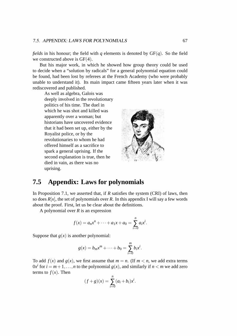
7.5. APPENDIX: LAWS FOR POLYNOMIALS 67
fields in his honour; the field withq elements is denoted by GF(q). So the fieldwe constructed above is GF(4).
But his major work, in which he showed how group theory could be usedto decide when a “solution by radicals” for a general polynomial equation couldbe found, had been lost by referees at the French Academy (who were probablyunable to understand it). Its main impact came fifteen years later when it wasrediscovered and published.
As well as algebra, Galois wasdeeply involved in the revolutionarypolitics of his time. The duel inwhich he was shot and killed wasapparently over a woman; buthistorians have uncovered evidencethat it had been set up, either by theRoyalist police, or by therevolutionaries to whom he hadoffered himself as a sacrifice tospark a general uprising. If thesecond explanation is true, then hedied in vain, as there was nouprising.
7.5 Appendix: Laws for polynomials
In Proposition 7.1, we asserted that, ifR satisfies the system (CRI) of laws, thenso doesR[x], the set of polynomials overR. In this appendix I will say a few wordsabout the proof. First, let us be clear about the definitions.
A polynomial overR is an expression
f (x) = anxn + · · ·+a1x+a0 =n
∑i=0
aixi .
Suppose thatg(x) is another polynomial:
g(x) = bmxm+ · · ·+b0 =m
∑i=0
bixi .
To add f (x) andg(x), we first assume thatm= n. (If m< n, we add extra terms0xi for i = m+1, . . . ,n to the polynomialg(x), and similarly ifn < mwe add zeroterms tof (x). Then
( f +g)(x) =n
∑i=0
(ai +bi)xi .

68 CHAPTER 7. POLYNOMIALS REVISITED
The rule for multiplication is a bit more complicated:
( f g)(x) =m+n
∑i=0
cixi ,
whereci = ∑a jbi− j ,
the sum being over all values ofj for which botha j andbi− j are defined; that is,we have 0≤ j ≤ n and 0≤ i− j ≤ m, so thati−m≤ j ≤ i. We can summarisethese two sets of conditions by saying
max(0, i−m)≤ j ≤min(i,n).
Consider, for example, the distributive law
( f +g)h = f h+gh.
We assume thatf andg are as above (withm= n) and that
h(x) =p
∑i=0
dixi .
Then the coefficient ofxi in ( f +g)h is
∑(a j +b j)di− j = ∑a jdi− j +b jdi− j ,
using the distributive law forR; and the coefficient inf h+gh is
∑a jdi− j +∑b jdi− j .
Now all the sums are over the same range max(0, i −m) ≤ j ≤ min(i, p), andrearranging the terms shows that the two expressions are equal.
Exercises
7.1 Suppose thatax+ b dividescnxn + · · ·+ c0 in Z[x], wherea,b,c0, . . . ,cn areintegers. Show thata dividescn, andb dividesc0. Hence show thatxn− 2 isirreducible overZ for any positive integern.
7.2 (a) Show that the polynomialx2 +1 is irreducible overZ3.
(b) Construct a field with nine elements.
7.3 Verify the associative law for multiplication of polynomials.

Chapter 8
Rings
We have seen many different types of structure (numbers, matrices, polynomials,sets, modular arithmetic) which satisfy very similar laws. Now we take the ob-vious next step: we consider systems satisfying these laws abstractly, and provethings about them directly from the laws they satisfy. The results will then be truein our systems no matter what they are made up of. This is called theaxiomaticmethod.
8.1 Rings
A ring is a setR of elements with two operations,addition(written+) andmulti-plication (written · or just by juxtaposing the factors) which satisfies the followinglaws. (Most of these we have seen before, but we state them all formally here.)
Additive laws:
(A0) Closure law: For ala,b∈ R, we havea+b∈ R.
(A1) Associative law: For alla,b,c∈ R, we havea+(b+c) = (a+b)+c.
(A2) Zero law: There is an element 0∈Rwith the property thata+0= 0+a= afor all a∈ R.
(A3) Additive inverse law: For alla∈ R, there exists an elementb∈ R such thata+b = b+a = 0. We writeb as−a.
(A4) Commutative law: For alla,b∈ R, we havea+b = b+a.
Multiplicative laws:
(M0) Closure law: For ala,b∈ R, we haveab∈ R.
69

70 CHAPTER 8. RINGS
(M1) Associative law: For alla,b,c∈ R, we havea(bc) = (ab)c.
Mixed laws:
D Distributive laws: For alla,b,c∈R, we havea(b+c) = ab+acand(b+c)a=ba+ca.
Before we go further, a couple of comments:
• The closure laws are new. Strictly speaking, they are not necessary, since tosay that+ is an operation onR means that the outputa+b when we inputa andb to the black box belongs toR. We put them in as a reminder that,when we are checking that something is a ring, we have to be sure that thisholds.
• We have stated the identity and inverse laws for addition in a more compli-cated way than necessary. Since we are going on to state the commutativelaw for addition, we could simply have said thata+0= a anda+(−a) = 0.We’ll see the reason soon.
We have already seen that sometimes the multiplication satisfies further laws,which resemble the laws for addition. This won’t always be the case, so we givespecial names to rings in which these laws hold.
Let Rbe a ring. We say thatR is aring with identityif
(M2) Identity law: There is an element 1∈R (with 1 6= 0) such that 1a = a1 = afor all a∈ R.
We say thatR is adivision ring if it satisfies (M2) and also
(M3) Multiplicative inverse law: for alla∈ R, if a 6= 0, then there existsb∈ Rsuch thatab= ba= 1. We writeb asa−1.
We say thatR is acommutative ringif
(M4) Commutative law: for alla,b∈ R, we haveab= ba.
(Note that the word “commutative” here refers to the multiplication; the additionin a ring is always commutative.) Finally, we say thatR is a field if it satisfies(M2), (M3) and (M4).
The condition (CRI) which we introduced in the last chapter thus stands for“commutative ring with identity”.
In a non-commutative ring, we need to assume both parts of the identity andmultiplicative inverse laws, since one does not follow from the other. Similarly,we do need both parts of the distributive law.

8.2. EXAMPLES OF RINGS 71
8.2 Examples of rings
We have a ready-made stock of examples:
• Z is a commutative ring with identity.
• Q, R andC are fields.
• If R is a commutative ring with identity, then so is thepolynomial ring R[x].
• If R is a ring, then so is the setMn×n(R) of all n×n matrices overR(with theusual definitions of matrix addition and multiplication). IfRhas an identity,then so doesMn×n(R). But this ring is usually not commutative.
• For anym, the setZm of integers modm is a commutative ring with identity.It is a field if and only ifm is prime.
• If R is a field andg(x) a monic polynomial of degree at least 1 overR, thenthe set of congruence classes of polynomals modg(x) is a commutative ringwith identity. It is a field if (and only if)g(x) is an irreducible polynomial.
Note that the third and fourth of these constructions (polynomials and matri-ces) are methods of building new rings from old ones. You may guess that thefifth and sixth can also be made into constructions of new rings from old. This iscorrect, but the construction is beyond the scope of this course. You will meet itnext year in Algebraic Structures I.
Some other familiar structures do not form rings. For example, the set ofnatural numbersN is not a ring, since the additive inverse law does not hold.
At the end of the last chapter, we constructed a field with four elements.
8.3 Properties of rings
We now give a few properties of rings. Since we only use the ring axioms in theproofs, and not any special properties of the elements, these are valid for all rings.This is the advantage of the axiomatic method.
Proposition 8.1 In a ring R,
there is a unique zero element;
any element has a unique additive inverse.

72 CHAPTER 8. RINGS
Proof (a) Suppose thatz andz′ are two zero elements. This means that, for anya∈ R,
a+z= z+a = a,
a+z′ = z′+a = a.
Now we havez+z′ = z′ (puttinga= z′ in the first equation) andz+z′ = z (puttinga = z in the second). Soz= z′.
This justifies us in calling the unique zero element 0.
(b) Suppose thatb andb′ are both additive inverses ofa. This means that
a+b = b+a = 0,
a+b′ = b′+a = 0.
Henceb = b+0 = b+(a+b′) = (b+a)+b′ = 0+b′ = b′.
(Here the first and last equalities hold because 0 is the zero element; the secondand second last are our assumptions aboutb andb′; and the middle equality is theassociative law.
This justifies our use of−a for the unique inverse ofa.
Proposition 8.2 Let R be a ring.
(a) If R has an identity, then this identity is unique.
(b) If a∈ R has a multiplicative inverse, then this inverse is unique.
The proof is almost identical to that of the previous proposition, and is left asan exercise.
The next result is called thecancellation law.
Proposition 8.3 Let R be a ring. If a+b = a+c, then b= c.
Proof
b= 0+b=(−a+a)+b=−a+(a+b)=−a+(a+c)= (−a+a)+c= 0+c= c.
Here the third and fifth equalities use the associative law, and the fourth is whatwe are given. To see where this proof comes from, start witha+b = a+c, thenadd−a to each side and work each expression down using the associative, inverseand zero laws.

8.3. PROPERTIES OF RINGS 73
Remark Try to prove that, ifR is a field anda 6= 0, thenab= ac impliesb = c.The next result is something you might have expected to find amongst our
basic laws. But it is not needed there, since we can prove it!
Proposition 8.4 Let R be a ring. For any element a∈ R, we have0a = a0 = 0.
Proof We have 0+0 = 0, since 0 is the zero element. Multiply both sides bya:
a0+a0 = a(0+0) = a0 = a0+0,
where the last equality uses the zero law again. Now froma0+a0 = a0+0, wegeta0 = 0 by the cancellation law. The other part 0a = 0 is proved similarly; tryit yourself.
There is one more fact we need. This fact uses only the associative law in itsproof, so it holds for both addition and multiplication. To state it, we take◦ to bea binary operation on a setX, which satisfies the associative law. That is,
a◦ (b◦c) = (a◦b)◦c
for all a,b,c∈ X. This means that we can writea◦b◦c without ambiguity.What about applying the operation to four elements? We have to put in brack-
ets to specify the order in which the operation is applied. There are five possibili-ties:
a◦ (b◦ (c◦d))a◦ ((b◦c)◦d)(a◦b)◦ (c◦d)(a◦ (b◦c))◦d
((a◦b)◦c)◦d
Now the first and second are equal, sinceb◦ (c◦ d) = (b◦ c) ◦ d. Similarly thefourth and fifth are equal. Consider the third expression. If we putx = a◦ b,then this expression isx◦ (c◦ d), which is equal to(x◦ c) ◦ d, which is the lastexpression. Similarly, puttingy = c◦d, we find it is equal to the first. So all fiveare equal.
This result generalises:
Proposition 8.5 Let ◦ be an operation on a set X which satisfies the associativelaw. Then the value of the expression
a1◦a2◦ · · · ◦an
is the same, whatever (legal) way n−2 pairs of brackets are inserted.
I won’t give the inductive proof here; you are encouraged to try it yourself!You will find the proof in an appendix to the notes.

74 CHAPTER 8. RINGS
8.4 Units
Let R be a ring with identity element 1. An elementu∈ R is called aunit if thereis an elementv∈ R such thatuv= vu= 1. The elementv is called theinverseofu, writtenu−1. By Proposition 8.2, a unit has a unique inverse.
Here are some properties of units.
Proposition 8.6 Let R be a ring with identity.
(a) 0 is not a unit.
(b) 1 is a unit; its inverse is1.
(c) If u is a unit, then so is u−1; its inverse is u.
(d) If u and v are units, then so is uv; its inverse is v−1u−1.
Proof (a) Since 0v = 0 for all v∈ R and 06= 1, there is no elementv such that0v = 1.
(b) The equation 1·1 = 1 shows that 1 is the inverse of 1.
(c) The equationu−1u = uu−1 = 1, which holds becauseu−1 is the inverse ofu, also shows thatu is the inverse ofu−1.
(d) Suppose thatu−1 andv−1 are the inverses ofu andv. Then
(uv)(v−1u−1) = u(vv−1)u−1 = u1u−1 = uu−1 = 1,
(v−1u−1)(uv) = v−1(u−1u)v = v−11v = v−1v = 1,
sov−1 is the inverse ofuv.
Here is how Hermann Weyl explains Proposition refunits(d), the statementthat (uv)−1 = v−1u−1, in his bookSymmetry, published by Princeton UniversityPress.
With this rule, although perhaps not with itsmathematical expression, you are all familiar. Whenyou dress, it is not immaterial in which order youperform the operations; and when in dressing youstart with the shirt and end up with the coat, then inundressing you observe the opposite order; first takeoff the coat and the shirt comes last.
Here are some examples of units in familiar rings.

8.4. UNITS 75
• In a field, every non-zero element is a unit.
• In Z, the only units are 1 and−1.
• Let F be a field. Then a polynomial in the polynomial ringF [x] is a unit ifand only if it is a non-zero constant polynomial. For we have
deg( f (x)g(x)) = deg( f (x))+deg(g(x)),
so if f (x)g(x) = 1 then f (x) must have degree zero, that is, it is a constantpolynomial.
• LetF be a field andna positive integer. An elementAof the ringMn×n(F) is
a unit if and only if the determinant ofA is non-zero. In particular,
(a bc d
)is a unit inM2×2(R) if and only if ad−bc 6= 0; if this holds, then its inverseis
1ad−bc
(d −b−c a
).
• Which elements are units in the ringZm of integers modm? The next resultgives the answer.
Proposition 8.7 Suppose that m> 1.
(a) An element[a]m of Zm is a unit if and only ifgcd(a,m) = 1.
(b) If gcd(a,m) > 1, then there exists b6≡m 0 such that[a]m[b]m = [0]m.
Proof Suppose that gcd(a,m) = 1; we show thata is a unit. By Euclid, there existintegersx andysuch thatax+my= 1. This meansax≡m 1, so that[a]m[x]m= [1]m,and[a]m is a unit.
Now suppose that gcd(a,m) = d > 1. Thena/d andm/d are integers, and wehave
a(m
d
)=
(ad
)≡m 0,
so[a]m[b]m = [0]m, whereb = m/d. Since 0< b < m, we have[b]m 6= [0]m.But this equation shows thata cannot be a unit. For, if[x]m[a]m = [1]m, then
[b]m = [1]m[b]m = [x]m[a]m[b]m = [x]m[0]m = [0]m,
a contradiction.

76 CHAPTER 8. RINGS
Example The table shows, for each non-zero element[a]12 of Z12, an element[b]12 such that the product is either 1 or 1. To save space we writea instead of[a]12.
a 1 2 3 4 5 6 7 8 9 10 11ab 1·1 = 1 2·6 = 0 3·4 = 0 4·3 = 0 5·5 = 1 6·2 = 0 7·7 = 1 8·3 = 0 9·4 = 0 10@cdot6 = 0 11·11= 1
Unit? √ × × × √ × √ × × × √
So the units inZ12 are[1]12, [5]12, [7]12, and[11]12.Euler’s functionφ(m), sometimes calledEuler’s totient function, is defined to
be the number of integersa satisfying 0≤ a≤ m− 1 and gcd(a,m) = 1. Thusφ(m) is the number of units inZm.
8.5 Appendix: The associative law
In this section we give the proof that, if◦ is an operation on a setX which satisfiesthe associative law, then the composition ofn terms doesn’t depend on how weput in the brackets (Proposition 8.5).
The proof is by induction onn. For n = 2, there are no brackets ina1 ◦ a2,and nothing to prove. Forn = 3, there ae two ways to put in the brackets, viz.a1◦ (a2◦a3) and(a1◦a2)◦a3; the associative law asserts that they are equal. Inthe notes we saw that, forn= 4, there are five bracketings, and the five expressionsare all equal.
So now suppose that the statement is true for expressions with fewer thannterms, and consider any two bracketings ofa1◦ · · · ◦an. Now for any bracketing,when we work it out “from the inside out”, in the last step we have just twoexpressions to be composed; that is, the expression looks like
(x1◦ · · · ◦xk)◦ (xk+1◦ · · · ◦xn).
There may be further brackets inside the two terms, but (according to the inductivehypothesis) they don’t affect the result. We will say that the expressionsplits afterk terms.
Suppose that the first expression splits afterk terms, and the second splits afterl terms.
Casek = l Both expressions now have the form
(x1◦ · · · ◦xk)◦ (xk+1◦ · · · ◦xn),
and by induction the bracketed terms don’t depend on any further brackets. Sothey are equal.

8.5. APPENDIX: THE ASSOCIATIVE LAW 77
Casek < l Now the first expression is
(x1◦ · · · ◦xk)◦ (xk+1◦ · · · ◦xn)
and the second is(x1◦ · · · ◦xl )◦ (xl+1◦ · · · ◦xn).
By the induction hypothesis, the value of the termx1 ◦ · · · ◦ xk doesn’t depend onwhere the brackets are; so we can rearrange the brackets so that this expressionsplits afterk terms, so that the whole expression is
((x1◦ · · · ◦xk)◦ (xk+1◦ · · · ◦xl ))◦ (xl+1◦ · · · ◦xn).
In the same way, we can rearrange the second expression as
(x1◦ · · · ◦xk)◦ ((xk+1◦ · · · ◦xl )◦ (xl+1◦ · · · ◦xn)).
Now the two expressions are of the form(a◦b)◦c anda◦ (b◦c), where
a = x1◦ · · · ◦xk,
b = xk+1◦ · · · ◦xl ,
c = xl+1◦ · · · ◦xn.
The associative law shows that they are equal.
Casek > l This case is almost identical to the preceding one.
Exercises
8.1 LetnZ be the set of all integers divisible byn. Show thatnZ is a ring (with theusual addition and multiplication). Is it commutative? Does it have an identity?
8.2 Let P(S) denote the set of all subsets of the setS. ForA,B∈P(S), defineA+B = A4B (symmetric difference), andAB= A∩B (intersection). Show thatP(S) is a ring. Show also thatA2 = A for all A∈P(S).
8.3 Let Rbe a ring in whicha2 = a for all a∈ R. By considering(a+b)2, show
(a) R is commutative;
(b) a+a = 0 for all a∈ R.
(Such a ring is called aBoolean ring.)

78 CHAPTER 8. RINGS

Chapter 9
Groups
The additive and multiplicative axioms for rings are very similar. This similaritysuggests considering a structure with a single operation, called a group. In thissection we study groups and their properties.
9.1 Definition
A group is a setG with an operation◦ onG satisfying the following axioms:
(G0) Closure law: for alla,b∈G, we havea◦b∈G.
(G1) Associative law: for alla,b,c∈G, we havea◦ (b◦c) = (a◦b)◦c.
(G2) Identity law: there is an elemente∈G (called theidentity) such thata◦e=e◦a = a for anya∈G.
(G3) Inverse law: for alla ∈ G, there existsb ∈ G such thata◦b = b◦a = e,wheree is the identity. The elementb is called theinverseof a, writtena′.
If in addition the following law holds:
(G4) Commutative law: for alla,b∈G we havea◦b = b◦a
thenG is called acommutative group, or more usually anabelian group(after theNorwegian mathematician Niels Abel).
9.2 Elementary properties
Many of the simple properties work in the same way as for rings.
Proposition 9.1 Let G be a group.
79

80 CHAPTER 9. GROUPS
(a) The composition of n elements has the same value however the brackets areinserted.
(b) The identity of G is unique.
(c) Each element has a unique inverse.
(d) Cancellation law; if a◦b = a◦c then b= c.
Proof (a) Proved in the appendix to the last section of the notes. (b) Ife ande∗
are identities thene= e◦e∗ = e∗.
(c) If b andb∗ are inverses ofa then
b = b◦e= b◦a◦b∗ = e◦b∗ = b∗.
(d) If ab= ac, multiply on the left by the inverse ofa to getb = c.
9.3 Examples of groups
We have some ready-made examples.
• Let R be a ring. TakeG = R, with operation+; the identity is 0 and theinverse ofa is−a. This group is called theadditive groupof the ringR. Itis an abelian group.
• Let Rbe a ring with identity, and letU(R) denote the set of units ofR, withoperation multiplication inR. This is a group;
– the closure, identity and inverse laws follow from Proposition xx inthe last part of the notes;
– the associative law follows from the ring axiom (M1).
This group is called thegroup of unitsof R. The next couple of examplesare special cases.
• In particular, ifF is a field, then the groupU(F) of units ofF consists of allthe non-zero elements ofF . This is called themultiplicative groupof F .

9.4. CAYLEY TABLES 81
• Let F be a field andn a positive integer. The setMn×n(F) of all n× nmatrices with elements inF is a ring. We saw that a matrix is a unit in thisring if and only if its determinant is non-zero. The groupU(Mn×n(F)) iscalled thegeneral linear groupof dimensionn overF , written GL(n,F).
• LetV be a vector space. Then, with the operation of vector addition,V is anabelian group; the identity is the zero vector0, and the inverse ofv is−v.
We will meet another very important class of groups in the next chapter.
Remark on notation I have used here a neutral symbol◦ for the group opera-tion. In books, you will often see the group operation written as multiplication, or(in abelian groups) as addition. Here is a table comparing the different notations.
Notation Operation Identity InverseGeneral a◦b e a′
Multiplicative ab, a·b 1 a−1
Additive a+b 0 −a
In order to specify the notation, instead of saying, “LetG be a group”, we oftensay, “Let(G,◦) (or (G,+), or (G, ·)) be a group”. The rest of the notation shouldthen be fixed as in the table.
Sometimes, however, the notations get a bit mixed up. For example, even withthe general notation, it is common to usea−1 instead ofa′ for the inverse ofa. Iwill do so from now on.
9.4 Cayley tables
If a group is finite, it can be represented by its operation table. In the case ofgroups, this table is more usually called theCayley table, after Arthur Cayley whopioneered its use. Here, for example, is the Cayley table of the group of units ofthe ringZ12.
· 1 5 7 111 1 5 7 115 5 1 11 77 7 11 1 511 11 7 5 1
Notice that, like the solution to a Sudoku puzzle, the Cayley table of a groupcontains each symbol exactly once in each row and once in each column (ignoringrow and column labels). Why? Suppose we are looking for the elementb in row a.It occurs in columnx if a◦x= b. This equation has the unique solutionx= a−1◦b,wherea−1 is the inverse ofa. A similar argument applies to the columns.
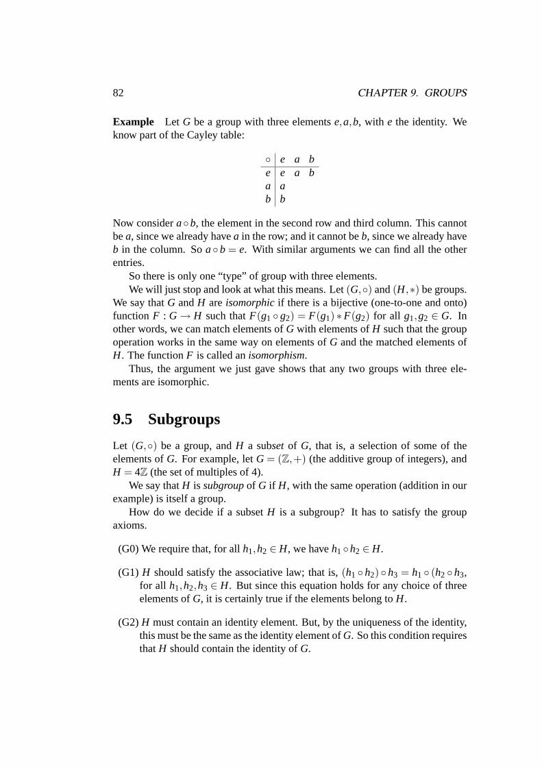
82 CHAPTER 9. GROUPS
Example Let G be a group with three elementse,a,b, with e the identity. Weknow part of the Cayley table:
◦ e a be e a ba ab b
Now considera◦b, the element in the second row and third column. This cannotbea, since we already havea in the row; and it cannot beb, since we already haveb in the column. Soa◦b = e. With similar arguments we can find all the otherentries.
So there is only one “type” of group with three elements.We will just stop and look at what this means. Let(G,◦) and(H,∗) be groups.
We say thatG andH areisomorphicif there is a bijective (one-to-one and onto)function F : G→ H such thatF(g1 ◦ g2) = F(g1) ∗F(g2) for all g1,g2 ∈ G. Inother words, we can match elements ofG with elements ofH such that the groupoperation works in the same way on elements ofG and the matched elements ofH. The functionF is called anisomorphism.
Thus, the argument we just gave shows that any two groups with three ele-ments are isomorphic.
9.5 Subgroups
Let (G,◦) be a group, andH a subset of G, that is, a selection of some of theelements ofG. For example, letG = (Z,+) (the additive group of integers), andH = 4Z (the set of multiples of 4).
We say thatH is subgroupof G if H, with the same operation (addition in ourexample) is itself a group.
How do we decide if a subsetH is a subgroup? It has to satisfy the groupaxioms.
(G0) We require that, for allh1,h2 ∈ H, we haveh1◦h2 ∈ H.
(G1) H should satisfy the associative law; that is,(h1 ◦h2) ◦h3 = h1 ◦ (h2 ◦h3,for all h1,h2,h3 ∈ H. But since this equation holds for any choice of threeelements ofG, it is certainly true if the elements belong toH.
(G2) H must contain an identity element. But, by the uniqueness of the identity,this must be the same as the identity element ofG. So this condition requiresthatH should contain the identity ofG.

9.6. COSETS AND LAGRANGE’S THEOREM 83
(G3) Each element ofH must have an inverse. Again by the uniqueness, thismust be the same as the inverse inG. So the condition is that, for anyh∈ H, its inverseh−1 belongs toH.
So we get one axiom for free and have three to check. But the amount of workcan be reduced. The next result is called theSubgroup Test.
Proposition 9.2 A non-empty subset H of a group(G,◦) is a subgroup if and onlyif, for all h1,h2 ∈ H, we have h1◦h−1
2 ∈ H.
Proof If H is a subgroup andh1,h2 ∈ H, thenh−12 ∈ H, and soh1◦h−1
2 ∈ H.Conversely suppose this condition holds. SinceH is non-empty, we can choose
some elementh∈ H. Takingh1 = h2 = h, we find thate= h◦h−1 ∈ H; so (G2)holds. Now, for anyh∈ H, we haveh−1 = e◦h−1 ∈ H; so (G3) holds. Then foranyh1,h2 ∈ H, we haveh−1
2 ∈ H, soh1 ◦h2 = h1 ◦ (h−12 )−1 ∈ H; so (G0) holds.
As we saw, we get (G1) for free.
In our example,G = Z, H = 4Z, take two elements ofH, say 4a and 4b; thensince the group operation is+, the inverse of 4b is −4b, and we have to checkwhether 4a−4b∈H. The answer is yes, since 4a−4b = 4(a−b) ∈ 4Z. So 4Z isa subgroup.
9.6 Cosets and Lagrange’s Theorem
In our example above, we saw that 4Z is a subgroup ofZ. Now Z can be parti-tioned into four congruence classes mod 4, one of which is the subgroup 4Z. Wenow generalise this to any group and any subgroup.
Let G be a group andH a subgroup ofG. Define a relation∼ onG by
g1 ∼ g2 if and only if g2◦g−11 ∈ H.
We claim that∼ is an equivalence relation.
reflexive:g1◦g−11 = e∈ H, sog1 ∼ g1.
symmetric: Letg1 ∼ g2, so thath = g2◦g−11 ∈ H. Thenh−1 = g1◦g−1
2 ∈ H, sog2 ∼ g1.
transitive: Suppose thatg1 ∼ g2 andg2 ∼ g3. Thenh = g2 ◦g−11 ∈ H andk =
g3◦g−12 ∈ H. Then
k◦h = (g3◦g−12 )◦ (g2◦g−1
1 ) = g3◦g−11 ∈ H,
sog1 ∼ g3.

84 CHAPTER 9. GROUPS
Now since we have an equivalence relation onG, the setG is partitioned intoequivalence classes for the relation. These equivalence classes are calledcosetsof H in G, and the number of equivalence classes is theindexof H in G, written|G : H|.
What do cosets look like?For anyg∈G, let
H ◦g = {h◦g : h∈ H}.
We claim that any coset has this form. Takeg∈ G, and letX be the equivalenceclass of∼ containingg. That is,X = {x∈G;g∼ x}.
• Takex∈ X. Theng∼ x, sox◦g−1 ∈ H. Let h = x◦g−1. Thenx = h◦g∈H ◦g.
• Take an element ofH ◦g, sayh◦g. Then(h◦g)◦g−1 = h∈H, sog∼ h◦g;thush◦g∈ X.
So every equivalence class is of the formH ◦g. We have shown:
Theorem 9.3 Let H be a subgroup of G. Then the cosets of H in G are the sets ofthe form
H ◦g = {h∈ g : h∈ H}
and they form a partition of G.
Example Let G = Z andH = 4Z. Since the group operation is+, the cosets ofH are the setsH +a for a∈ G, that is, the congruence classes. There are four ofthem, so|G : H|= 4.
Remark We write the coset asH ◦g, and call the elementg thecoset represen-tative. But any element of the coset can be used as its representative. In the aboveexample,
4Z+1 = 4Z+5 = 4Z−7 = 4Z+100001= · · ·
If G is finite, theorder of G is the number of elements ofG. (If G is infinite,we sometimes say that it has infinite order.) We write the order ofG as|G|.
Now the partition into cosets allows us to prove an important result,La-grange’s Theorem:
Theorem 9.4 Let G be a finite group, and H a subgroup of G. Then|H| divides|G|. The quotient|G|/|H| is equal to|G : H|, the index of H in G.

9.7. ORDERS OF ELEMENTS 85
Proof We know thatG is partitioned into the cosets ofH. If we can show thateach coset has the same number as elements asH does, then it will follow that thenumber of cosets is|G|/|H|, and the theorem will be proved.
So letH ◦g be a coset ofH. We define a functionf : H → H ◦g by the rulethat f (h) = h◦g. We show thatf is one-to-one and onto. Then the conclusionthat|H ◦g|= |H| will follow.
f is one-to-one: suppose thatf (h1) = f (h2), that is,h1 ◦ g = h2 ◦ g. By theCancellation Law,h1 = h2.
f is onto: take an elementx∈ H ◦g, sayx = h◦g. Thenx = f (h), as required.
9.7 Orders of elements
Remember that the order of a group is the number of elements in the group. Wewill define in this section the order of an element of a group. This is quite different– be careful not to get them confused – but there is a connection, as we will see.
Let g be an element of a groupG. We definegn for every integern in thefollowing way:
g0 = e,
gn = gn−1◦g for n > 0,
g−n = (gn)−1 for n > 0.
Now it is possible to prove that theexponent lawshold:
Proposition 9.5 For any integers m and n,
(a) gm◦gn = gm+n,
(b) (gm)n = gmn.
The proof is not difficult but needs a lot of care. It follows from the definitionthat
gn ={
g◦ · · · ◦g (n factors) ifn > 0,g−1◦ · · · ◦g−1 (−n factors) ifn < 0.
Now considergm+n. There are four cases.
• If m andn are both positive then
gm◦gn = g◦ · · · ◦g (m+n factors)= gm+n.

86 CHAPTER 9. GROUPS
• If one ofm andn is positive, saym> 0, n < 0, then
– If m+ n > 0, so thatm> −n, then−n of the factorsg cancel all thefactorsg−1, leavingm+n factorsg, so the result isgm+n.
– If m+n < 0, thenmof the factorsg−1 cancel all the factorsg, leaving−m−n factorsg−1; again we havegm+n.
• Finally, if m andn are both negative, a similar argument to the first caseapplies.
If one ofm andn is zero, saym= 0, then the product ise◦gn = gn.The argument for the second exponent law is similar.
It follows from the second exponent law that(gn)−1 = g−n. This also followsbecausegn◦g−n = g0 = e.
Now we make two definitions.
• The order of the elementg is the smallest positive numbern for whichgn = e, if such a number exists; if no positive power ofg is equal toe, wesay thatg has infinite order.
• Thesubgroup generated by gis the set
{gn : n∈ Z}
of all powers ofg. We write it as〈g〉.
It is not clear from what has been said so far that “the subgroup generated byg” is actually a subgroup! In fact it is; this and more are contained in the nextProposition. Remember that the word “order” has two different meanings; thefirst is the number of elements in the subgroup, the second is the number we havejust defined.
Proposition 9.6 For any element g of a group G, the set〈g〉 is a subgroup of G,and its order is equal to the order of g.
Proof To show that〈g〉 is a subgroup, we apply the Subgroup Test. Take twoelements of this set, saygm andgn. Then
gm◦ (gn)−1 = gm◦g−n = gm−n ∈ 〈g〉.
Next we show that, ifg has ordern, then
• gm = e if and only if n dividesm;

9.8. CYCLIC GROUPS 87
• gk = gl if and only if k≡n l .
Suppose thatm= nq. Thengm = (gn)q = eq = e. Conversely, suppose thatgm = e.By the Division Rule,m= nq+ r, with 0≤ r ≤ n−1. Nowgn = gm = e, sogr = e.But n is the smallest positive integer such that thenth power ofg is e; sincer < nwe must haver = 0, andn dividesm.
Now gk = gl if and only if gl−k = e. By the preceding paragraph, this holds ifand only ifn dividesl −k, that is, if and only ifk≡n l .
We see that ifg has ordern, then the set〈g〉 contains justn elements (one foreach congruence class modn), so it is a subgroup of ordern.
Similarly, if g has infinite order, then all the elements of〈g〉 are distinct (sinceif gk = gl thengl−k = e), so〈g〉 is an infinite subgroup.
Corollary 9.7 Let g be an element in a finite group of order n. Then gn = e.
Proof The order ofg cannot be infinite, since〈g〉 is a finite set in this case. Sup-pose the order ofg is m. Then the order of the subgroup〈g〉 is m. By Lagrange’sTheorem,m dividesn = |G|.
Now we can revisit Fermat’s Little Theorem and prove a stronger version.
Proposition 9.8 Let n be a positive integer, and a an integer such thatgcd(a,n) =1. Then aφ(n) ≡n 1, whereφ is Euler’s totient function.
Proof Let Un be the group of units ofZn. Then|Un| = φ(n), and[a]n ∈Un. By
the preceding corollary,[aφ(n)]n = [a]φ(n)n = [1]n; in other words,aφ(n) ≡n 1.
Example There are four units inZ12, namely 1,5,7,11. (We writea instead of[a]12.) By the Corollary, ifa is one of these four numbers, thena4 ≡12 1. In fact,in this casea2 ≡12 1 for each of the four numbers.
9.8 Cyclic groups
A groupG is acyclic groupif G = 〈g〉 for some elementg∈G.The prototypical cyclic group of ordern is (Zn,+), while the prototypical
infinite cyclic group is(Z,+). In each case, the group is generated by the element1.
Proposition 9.9 Any two cyclic groups of the same order are isomorphic.
88 CHAPTER 9. GROUPS
Proof We show that a cyclic group of ordern is isomorphic toZn, while aninfinite cyclic group is isomorphic toZ.
Let G = 〈g〉 be a cyclic group of ordern. We saw in the last section that theelementg has ordern, and thatgk = gl if and only if k≡n l . Now the map[k]n 7→ gk
is well-defined and is one-to-one and onto, that is, a bijection, fromZn to G; andit is an isomorphism, since
gk ◦gl = gm⇔ k+ l ≡n m.
The proof for infinite groups is even simpler and is left to you.
Exercises
9.1 Show that, ifb◦a = c◦a, thenb = c.
9.2 Let G be a group of ordern. Show thatG is a cyclic group if and only ifGcontains an element whose order isn. Hence show that any group of prime orderis cyclic.
9.3 Let G be a group of order 4; sayG = {e,a,b,c}, wheree is the identity.Suppose thatG is not a cyclic group.
(a) Show thata2 = b2 = c2 = e.
(b) Determine the Cayley table ofG.
(c) Show thatG is abelian.

Chapter 10
Permutations
We have seen rings and groups whose elements are numbers, polynomials, matri-ces, and sets. In this chapter we meet another type of object: permutations. Theoperation on permutations is composition, and we construct groups of permuta-tions which play and important role in general group theory.
10.1 Definition and representation
A permutationof a setX is a functionf : X → X which is a bijection (one-to-oneand onto).
In this section we consider only the case whenX is a finite set, and we takeX to be the set{1,2, . . . ,n} for convenience. As an example of a permutation, wewill take n = 8 and letf be the function which maps 17→ 4, 2 7→ 7, 3 7→ 3, 4 7→ 8,5 7→ 1, 6 7→ 5, 7 7→ 2, and 87→ 6.
We can represent a permutation intwo-line notation. We write a matrix withtwo rows andn columns. In the first row we put the numbers 1, . . . ,8; under eachnumberx we put its image under the permutationf . In our example, we have
f =(
1 2 3 4 5 6 7 84 7 3 8 1 5 2 6
).
How many permutations of the set{1, . . . ,n} are there? We can ask this ques-tion another way? How many matrices are there with two rows andn columns,such that the first row has the numbers 1, . . . ,n in order, and the second containsthesen numbers in an arbitrary order? There aren choices for the first element inthe second row; thenn−1 choices for the second element (since we can’t re-usethe element in the first column); thenn−2 for the third; and so on until the lastplace, where the one remaining number has to be put. So altogether the number
89

90 CHAPTER 10. PERMUTATIONS
of permutations isn· (n−1) · (n−2) · · ·1.
This number is calledn! (read “n factorial” or “factorial n”), the product of thenatural numbers from 1 ton. Thus we have proved:
Proposition 10.1 The number of permutations of the set{1, . . . ,n} is n! .
10.2 The symmetric group
Let f1 and f2 be permutations. We define thecompositionof f1 and f2 to be thepermutation obtained by applyingf1 and thenf2.
Warning If you write the image ofx under the permutationf as f (x), then thecomposition off1 and f2 mapsx to f2( f1(x)) – note the reversal! In order to makethe notation work better, we change the way we write the image ofx under f byputting f on the right, asx f (or sometimes up in the air, asxf ). Then we havex( f1◦ f2) = (x f1) f2, which is easier to remember.
You should be aware, though, that some people choose to resolve the problemthe other way, by defining the composition off1 and f2 to be “first f2, then f1”.
In practice, how do we compose permutations? (Practice is the right wordhere: you should practise composing permutations until you can do it withoutstopping to think.) Letf be the permutation we used as an example in the lastsection, and let
g =(
1 2 3 4 5 6 7 83 2 1 8 7 6 5 4
).
The easiest way to calculatef ◦g is to take each of the numbers 1, . . . ,8, map itby f , map the result byg, and write down the result to get the bottom row of thetwo-line form for f ◦g. Thus, f maps 1 to 4, andg maps 4 to 8; sof ◦g maps 1 to8; f maps 2 to 7, andg maps 7 to 5, sof ◦g maps 2 to 5; and so on.
Another way to do it is to re-write the two-line form forg by shuffling thecolumns around so that the first row agrees with the second row off . Then thesecond row will be the second row off ◦g. Thus,
g =(
1 2 3 4 5 6 7 83 2 1 8 7 6 5 4
)=
(4 7 3 8 1 5 2 68 5 1 4 3 7 2 6
);
so
f ◦g =(
1 2 3 4 5 6 7 88 5 1 4 3 7 2 6
).
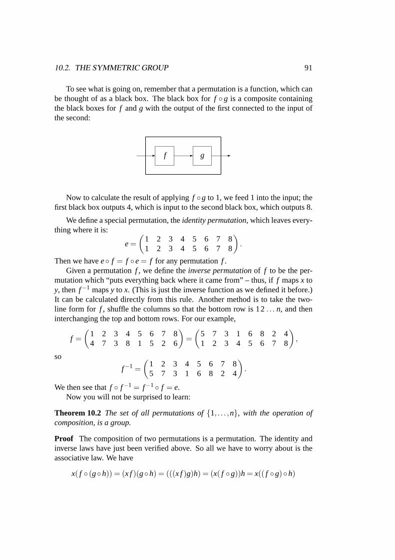
10.2. THE SYMMETRIC GROUP 91
To see what is going on, remember that a permutation is a function, which canbe thought of as a black box. The black box forf ◦g is a composite containingthe black boxes forf andg with the output of the first connected to the input ofthe second:
f g- - -
Now to calculate the result of applyingf ◦g to 1, we feed 1 into the input; thefirst black box outputs 4, which is input to the second black box, which outputs 8.
We define a special permutation, theidentity permutation, which leaves every-thing where it is:
e=(
1 2 3 4 5 6 7 81 2 3 4 5 6 7 8
).
Then we havee◦ f = f ◦e= f for any permutationf .Given a permutationf , we define theinverse permutationof f to be the per-
mutation which “puts everything back where it came from” – thus, iff mapsx toy, then f−1 mapsy to x. (This is just the inverse function as we defined it before.)It can be calculated directly from this rule. Another method is to take the two-line form for f , shuffle the columns so that the bottom row is 12. . . n, and theninterchanging the top and bottom rows. For our example,
f =(
1 2 3 4 5 6 7 84 7 3 8 1 5 2 6
)=
(5 7 3 1 6 8 2 41 2 3 4 5 6 7 8
),
so
f−1 =(
1 2 3 4 5 6 7 85 7 3 1 6 8 2 4
).
We then see thatf ◦ f−1 = f−1◦ f = e.Now you will not be surprised to learn:
Theorem 10.2 The set of all permutations of{1, . . . ,n}, with the operation ofcomposition, is a group.
Proof The composition of two permutations is a permutation. The identity andinverse laws have just been verified above. So all we have to worry about is theassociative law. We have
x( f ◦ (g◦h)) = (x f)(g◦h) = (((x f)g)h) = (x( f ◦g))h = x(( f ◦g)◦h)

92 CHAPTER 10. PERMUTATIONS
for all x; so f ◦ (g◦h) = ( f ◦g)◦h, the associative law.(Essentially, this last argument shows that the result of applyingf ◦ g◦ h,
bracketed in any fashion, is “f , theng, thenh”.)
We call this group thesymmetric group of degree n, and write itSn. Note thatSn is a group of ordern! .
Proposition 10.3 Sn is an abelian group if n≤ 2, and is non-abelian if n≥ 3.
Proof S1 has order 1, andS2 has order 2; it is easy to check that these groups areabelian, for example by writing down their Cayley tables.
For n≥ 3, Sn contains elementsf andg, where f interchanges 1 and 2 andfixes 3, . . . ,n, andg interchanges 2 and 3 and fixed 1, 4. . . ,n. Now check thatf ◦g 6= g◦ f . (For example,f ◦g maps 1 to 3, butg◦ f maps 1 to 2.)
10.3 Cycles
We come now to a way of representing permutations which is more compact thanthe two-line notation described earlier, but (after a bit of practice!) just as easy tocalculate with: this iscycle notation.
Let a1,a2, . . . ,ak be distinct numbers chosen from the set{1,2, . . . ,n}. Thecycle(a1,a2, . . . ,ak) denotes the permutation which mapsa1 7→ a2, a2 7→ a3, . . . ,ak−1 7→ ak, andak 7→ a1. If you imaginea1,a2, . . . ,ak written around a circle, thenthe cycle is the permutation where each element moves to the next place round thecircle. Any number not in the set{a1, . . . ,ak} is fixed by this manoeuvre.
Notice that the same permutation can be written in many different ways as acycle, since we may start at any point:
(a1,a2, . . . ,ak) = (a2, . . . ,ak,a1) = · · ·= (ak,a1, . . . ,ak−1).
If (a1, . . . ,ak) and (b1, . . . ,bl ) are cycles with the property that no elementlies in both of the sets{a1, . . . ,ak} and{b1, . . . ,bl}, then we say that the cyclesaredisjoint, and define theirproductto be the permutation which acts as the firstcycle on theas, as the second cycle on thebs, and fixes the other elements (ifany) of{1, . . . ,n}. In a similar way, we define the product of any set of pairwisedisjoint cycles.
Theorem 10.4 Any permutation can be written as a product of disjoint cycles.The representation is unique, up to the facts that the cycles can be written in anyorder, and each cycle can be started at any point.

10.3. CYCLES 93
Proof Our proof is an algorithm to find thecycle decompositionof a permutation.We will consider first our standard example:
f =(
1 2 3 4 5 6 7 84 7 3 8 1 5 2 6
).
Now we do the following. Start with the first element, 1. Follow its successiveimages underf until it returns to its starting point:
f : 1 7→ 4 7→ 8 7→ 6 7→ 5 7→ 1.
This gives us a cycle(1,4,8,6,5).If this cycle contains all the elements of the set{1, . . . ,n}, then stop. Other-
wise, choose the smallest unused element (in this case 2, and repeat the procedure:
f : 2 7→ 7 7→ 2,
so we have a cycle(2,7) disjoint from the first.We are still not finished, since we have not seen the element 3 yet. Nowf : 3→
3, so(3) is a cycle with a single element. Now we have the cycle decomposition:
f = (1,4,8,6,5)(2,7)(3).
The general procedure is the same. Start with the smallest element of the set,namely 1, and follow its successive images underf until we return to somethingwe have seen before. This can only be 1. For suppose thatf : 1 7→ a2 7→ · · · 7→ak 7→ as, where 1< s< k. Then we haveas−1 f = as = ak f , contradicting the factthat f is one-to-one. So the cycle ends by returning to its starting point.
Now continue this procedure until all elements have been used up. We cannotever stray into a previous cycle during this procedure. For suppose we start at anelementb1, and havef : b1 7→ · · · 7→ bk 7→ as, whereas lies in an earlier cycle.Then as before,as−1 f = as = bk f , contradicting the fact thatf is one-to-one. Sothe cycles we produce really are disjoint.
The uniqueness is hopefully clear.
You should practise composing and inverting permutations in disjoint cyclenotation. Finding the inverse is particularly simple: all we have to do to findf−1
is to write each cycle off in reverse order!We simplify the notation still further. Any element in a cycle of length 1 is
fixed by the permutation, and by convention we do not bother writing such cycles.So our example permutation could be written simply asf = (1,4,8,6,5)(2,7).The fact that 3 is not mentioned means that it is fixed. (You may notice that thereis a problem with this convention: the identity permutation fixes everything, andso would be written just as a blank space! We get around this either by writingone cycle(1) to represent it, or by just calling ite.)
Cycle notation makes it easy to get some information about a permutation:

94 CHAPTER 10. PERMUTATIONS
Proposition 10.5 The order of a permutation is the least common multiple of thelengths of the cycles in its disjoint cycle representation.
Proof Recall that the order off is the smallest positive integern such thatf n = e.To see what is going on, return to our standard example:
f = (()1,4,8,6,5)(2,7)(3).
Now elements in the first cycle return to their starting position after 5 steps, andagain after 10, 15, . . . steps. So, iff n = 1, thenn must be a multiple of 5. Butalso the elements 2 and 7 swap places iff is applied an odd number of times, andreturn to their original positions after an even number of steps. So iff n = 1, thenn must also be even. Hence iff n = 1 thenn is a multiple of 10. The point 3 isfixed by any number of applications off so doesn’t affect things further. Thus,the order ofn is a multiple of 10. Butf 10 = e, since applyingf ten times takeseach element back to its starting position; so the order is exactly 10.
In general, if the cycle lengths arek1,k2, . . . ,kr , then elements of theith cycleare fixed byf n if and only if n is a multiple ofki ; so f n = e if and only if n is amultiple of all ofk1, . . . ,kr , that is, a multiple of lcm(k1, . . . ,kr). So this lcm is theorder of f .
10.4 Transpositions
A transpositionis a permutation which swaps two elementsi and j and fixes allthe other elements of{1, . . . ,n}. In disjoint cycle form, a transposition looks like(i, j).
Theorem 10.6 Any permutation in Sn can be written as a product of transpo-sitions. The number of transpositions occurring in a product equal to a givenelement f is not always the same, but always has the same parity (even or odd)depending on g.
Proof We begin by observing that
(1,2, . . . ,n) = (1,2)(1,3) · · ·(1,n).
For, in the product on the right,
• 1 is mapped to 2 by the first factor, and remains there afterwards;
• 2 is mapped to 1 by the first factor, then to 2 by the second, then stays there;

10.4. TRANSPOSITIONS 95
• . . .
• n−1 is fixed by all factors until the second-last; it is mapped to 1 by thesecond-last factor and then ton by the last;
• n is fixed by all factors except the last, which takes it to 1.
So the two permutations are equal.Now in exactly the same way, an arbitrary cycle(a1,a2, . . . ,ak) can be written
as a product of transpositions:
(a1,a2, . . . ,ak) = (a1,a2)(a1,a3) · · ·(a1,ak).
Finally, given an arbitrary permutation, write it in disjoint cycle form, and thenwrite each cycle as a product of transpositions.
The statement about parity is harder to prove, and I have put the proof into anappendix.
Our standard example can be written
f = (1,4,8,6,5)(2,7) = (1,4)(1,8)(1,6)(1,5)(2,7).
We call a permutationevenor odd according as it is a product of an even orodd number of transpositions; we call this theparity of f . Notice that a cycle oflengthk is a product ofk−1 transpositions. So, if the lengths of the cycles offarek1, . . . ,kr (including fixed points), thenf is the product of
(k1−1)+(k2−1)+ · · ·+(kr −1) = n− r
transpositions (since the cycle lengths add up ton). In other words, if we definec( f ) to be the number of cycles in the cycle decomposition off , then the parityof f is the same as the parity ofn−c( f ).
Theorem 10.7 Suppose that n≥ 2. Then the set of even permutations in Sn is asubgroup of Sn having order n!/2 and index2.
Proof Let An be the set of even permutations inSn. If f1, f2 ∈ An, then f−12 has
the same cycle lengths asf2 (since we just reverse all the cycles), so it is also inAn. Thus, f1 and f−1
2 are each products of an even number of transpositions; andthen so, obviously, isf1◦ f−1
2 . By the Subgroup Test,An is a subgroup.Let ∼ be the equivalence relation defined by this subgroup; that is,f1 ∼ f2
if and only if f1 ◦ f−12 ∈ An. By considering each off1 and f2 as products of
transpositions, we see thatf1 ∼ f2 if and only if f1 and f2 have the same parity.So there are just two cosets ofAn.
By Lagrange’s Theorem,
|An|= |Sn|/2 = n!/2.

96 CHAPTER 10. PERMUTATIONS
The subgroupAn consisting of even permutations is called thealternatinggroupof degreen.
Example For n = 3, we have|S3| = 3! = 6, so|A3| = 3. The three even per-mutations aree, (1,2,3) and (1,3,2); the remaining three permutations are thetranspositions(1,2), (1,3) and(2,3) form the other coset ofA3 in S3.
Remark The formula for a 3×3 determinant can be expressed as follows. Foreach permutationf ∈ S3, we do the following. Pick the elements in rowi andcolumn i f of the matrix, and multiply them together. That is, choose one termfrom each row and column in all possible ways. Now multiply the product by+1if f is an even permutation, and by−1 if f is an odd permutation. Finally, add upthese terms for all the permutations.
For example, if
A =
a b cl m np q r
,
the terms are as follows:
Permutation Product Signe amr +
(1,2,3) bnp +(1,3,2) clq +(1,2) blr −(1,3) cmp −(2,3) anq −
So det(A) = amr+bnp+clq−blr−cmp−anq.
Now exactly the same procedure defines the determinant of ann×n matrix,for any positive integern. The drawback is that the number of terms needed for ann×n determinant isn!, a rapidly growing function; so the work required becomesunreasonable very quickly. This is not a practical way to compute determinants;but it is as good a definition as any!
10.5 Even and odd permutations
In this Appendix, we prove that the parity (even or odd) of a permutation does notdepend on the way we write it as a product of transpositions. We will give twoentirely different proofs.

10.5. EVEN AND ODD PERMUTATIONS 97
First proof
For this proof, we see what happens when we multiply a permutation by a trans-position. We find that the number of cycles changes by 1 (it may increase or de-crease). There are two cases, depending on whether the two points transposed liein different cycles or the same cycle of the permutation. So letf be a permutationandt a transposition.
Case 1: Transposing two points in different cycles. We may suppose thatf con-tains two cycles(a1, . . . ,ak) and(b1, . . . ,bl ), and thatt = (a1,b1) (this is becausewe can start each of the cycles at any point). Cycles off not containing pointsmoved byt will be unaffected. Now we find
f ◦ t : a1 7→ a2 7→ · · · 7→ ak 7→ b1 7→ b2 7→ · · · 7→ bl 7→ a1,
so the two cycles off are “stitched together” into a single cycle inf ◦ t, and thenumber of cycles decreases by 1.
Case 2: Transposing two points in the same cycle. This time let(a1, . . . ,am, . . . ,ak)be a cycle off , and assume thatt = (a1,am), where 1< m≤ k. This time
f ◦ t : a1 7→ a2 7→ · · · 7→ am−1 7→ a1
am 7→ am+1 7→ · · · 7→ ak 7→ am
so the single cycle off is “cut apart” into two cycles.
Now any permutationf can be written as
f = t1◦ t2◦ · · · ◦ ts,
wheret1, . . . , fs are transpositions. Letfi be the product of the firsti of the trans-positions, and consider the quantityn− c( fi), wherec( f ) denotes the number ofcycles of f (including fixed points). We start withf0 = e, havingn fixed points,son−c( f0) = 0. Now, at each step, we multiply by a transposition, so we changec( fi) by one, and hence changen− c( fi) by one. So the final valuen− c( f ) iseven or odd depending on whether the numbers of transpositions is even or odd.But n−c( f ) is defined just by the cycle decomposition off , independent of howwe express it as a product of transpositions. So in any such expression, the parityof the number of transpositions will be the same.

98 CHAPTER 10. PERMUTATIONS
Second proof
Let x1, . . . ,xn ben indeterminates, and consider the function
F(x1, . . . ,xn) = ∏i< j
(x j −xi).
For example, forn = 3, we have
F(x1,x2,x3) = (x2−x1)(x3−x1)(x3−x2).
Given a permutationf , we define a new functionF f of the same indetermi-nates by applying the permutationf to their indices:
F f (x1, . . . ,xn) = ∏i< j
(x j f −xi f ).
For example, ifn = 3 and f = (2,3), then
F(1,2)(x1,x2,x3) = (x3−x1)(x2−x1)(x2−x3) =−F(x1,x2,x3).
The result of applyingf1 and thenf2 to F is just the result of applyingf2◦ f1to F , as you may check. We show that, for any transpositiont, we have
F t(x1, . . . ,xn) =−F(x1, . . . ,xn).
It will follow that, if f is expressed as the product ofs transpositions, then
F f (x1, . . . ,xn) = (−1)sF(x1, . . . ,xn).
Since the value ofF f does not depend on which expression as a product of trans-positions we use, we see that(−1)s must be the same for all such expressions forf , and hence the number of transpositions in the product must always have thesame parity, as required.
To prove our claim, take the transpositiont = (k, l), wherek < l , and see whatit does toF . We look at the bracketed terms(x j − xi) and see what happens tothem. There are several cases.
• If {k, l}∩{i, j}= /0, then the term is unaffected by the permutationt.
• If i < k, then the terms(xk−xi) and(xl −xi) are interchanged, and there isno effect onF .
• If k < i < l , then the term(xi − xk) goes to(xi − xl ) = −(xl − xi), and theterm (xl − xi) goes to(xk− xi) = −(xi − xk); the two sign changes cancelout.

10.5. EVEN AND ODD PERMUTATIONS 99
• If i > l , then the terms(xi −xk) and(xi −xl ) are interchanged, and there isno effect onF .
• Finally, the term(x j −xi) is mapped to(xi −x j) =−(x j −xi).
So the overall effect oft is to introduce one minus sign, and we conclude thatF t =−F , as required.
Exercises
10.1 Let g = (1,5,4,9,6,3)(7,8) and h = (1,4,3)(6,8,7)(5,9,2) be permuta-tions in the symmetric groupS9. Findg◦h, g2, g−1, andg−1◦h◦g. Show thathandg−1◦h◦g have the same order.
10.2 If g andh are elements of any group, show that
(g−1◦h◦g)n = g−1◦hn◦g
for any integern, and deduce thath andg−1◦h◦g necessarily have the same order.
10.3 List the elements ofS4, and say whether each is an even or odd permutation.

Index
Abel, Niels, 79abelian group, 79addition, 69additive group, 80Al-Khwarizmi, iiialternating group, 96Argand diagram, 21associative law, 16, 70, 73, 76, 79
bijective, 41, 42blackboard bold, 15Boolean ring, 77Borel, Emil, 16
cancellation law, 72, 80Carroll, Lewis, 12Cartesian product, 36Cayley table, 81Cayley, Arthur, 81closure law, 70, 79commutative group, 79commutative law, 16, 17, 70, 79commutative ring, 70commutative ring with identity, 61complement, 33complex numbers, 19, 65complex plane, 21composition
of permutations, 90congruence, 55, 63conjecture, 11converse, 12coordinates, 35corollary, 10
coset, 84coset representative, 84counterexample, 7
minimal, 10CRI, 61cycle notation, 92cyclic group, 87
De Moivre’s Theorem, 23definition, 12degree
of polynomial, 31Descartes, Rene, 35determinant, 96difference
of sets, 33distributive law, 16, 17, 68, 70divides, 48division algorithm, 48division ring, 70division rule, 47, 51dot diagrams, 17
equivalence relation, 38Equivalence Relation Theorem, 39equivalent conditions, 6Euclid, 5Euclid’s algorithm, 49, 53Euclid’s Theorem, 5Euler’s function, 76even permutation, 95exponent laws, 85
Factor Theorem, 63
100

INDEX 101
factorial, 90Fermat’s Last Theorem, 11Fermat’s Little Theorem, 59, 87Fermat, Pierre, 11field, 64, 70, 71
finite, 66finite field, 66function, 40Fundamental Theorem of Algebra, 46
Galois field, 67Galois,Evariste, 67gcd, 48, 53general linear group, 81Goldbach’s conjecture, 11greatest common divisor, 48, 53group, 79
alternating, 96cyclic, 87symmetric, 92
group of units, 80
identity law, 16, 70, 79identity permutation, 91if, 6if and only if, 2, 6implied by, 6implies, 6index, 84induction, 7injective, 41, 42integers, 17intersection, 32inverse function, 42inverse law, 17, 70, 79inverse permutation, 91isomorphic, 82, 87isomorphism, 82
Johnson, Samuel, iii
Kronecker, Leopold, 16
Lagrange’s Theorem, 84laws, 16, 25lcm, 49least common multiple, 49lemma, 10
matrices, 28matrix addition, 28matrix multiplication, 28matrix ring, 71minimal counterexample, 10modular arithmetic, 57monic, 63monic polynomial, 52multiplication, 69multiplicative group, 80
natural numbers, 1, 16necessary and sufficient condition, 6necessary condition, 6
odd permutation, 95one-to-one, 41, 42one-to-one correspondence, 41only if, 6onto, 41, 42operation, 43order
of element, 86of group, 84of permutation, 94
ordered pair, 35
parityof permutation, 95
partition, 38permutation, 89polynomial, 31, 51, 62
monic, 63polynomial ring, 71prime numbers, 5proof, 11

102 INDEX
by contradiction, 3by induction, 7
proposition, 10Pythagoras, 3Pythagoras’ Theorem, 3
rational numbers, 3, 18real numbers, 19reflexive, 38relations, 37Remainder Theorem, 63ring, 69
Boolean, 77commutative with identity, 61
ring with identity, 70
scalar product, 27sets, 32subgroup, 82
generated by element, 86subgroup test, 83sufficient condition, 6surjective, 41, 42symmetric, 38symmetric difference, 33symmetric group, 92
theorem, 10totient function, 76, 87transitive, 38transposition, 94trigonometry, 23two-line notation
for permutation, 89
union, 32unit, 74unordered pair, 35
vector, 25, 81vector addition, 26vector product, 27
Venn diagrams, 32
Weyl, Hermann, 74Wiles, Andrew, 11Wilson’s Theorem, 59
zero law, 70