temporal variability in soil hydraulic properties under

HAL Id: hal-00547590https://hal.archives-ouvertes.fr/hal-00547590

Submitted on 16 Dec 2010

HAL is a multi-disciplinary open accessarchive for the deposit and dissemination of sci-entific research documents, whether they are pub-lished or not. The documents may come fromteaching and research institutions in France orabroad, or from public or private research centers.

L’archive ouverte pluridisciplinaire HAL, estdestinée au dépôt et à la diffusion de documentsscientifiques de niveau recherche, publiés ou non,émanant des établissements d’enseignement et derecherche français ou étrangers, des laboratoirespublics ou privés.

Temporal variability in soil hydraulic properties underdrip irrigation

I. Mubarak, J.C. Mailhol, Rafaël Angulo-Jaramillo, P. Ruelle, Pierre Boivin,M.R. Khaledian

To cite this version:I. Mubarak, J.C. Mailhol, Rafaël Angulo-Jaramillo, P. Ruelle, Pierre Boivin, et al.. Temporal vari-ability in soil hydraulic properties under drip irrigation. Geoderma, Elsevier, 2009, 150, p. 158 - p.165. �10.1016/j.geoderma.2009.01.022�. �hal-00547590�

https://hal.archives-ouvertes.fr/hal-00547590

https://hal.archives-ouvertes.fr

1

Geoderma, Volume 150, Issues 1-2, 15 April 2009, Pages 158-165 1 Author-produced version of the final draft post-reefering article. 2 Orginal version available at Elsevier B.V. doi:10.1016/j.geoderma.2009.01.022 3

4

Temporal variability in soil hydraulic properties under drip irrigation 5 IBRAHIM MUBARAK1,2,3*, JEAN CLAUDE MAILHOL2, RAFAEL ANGULO-JARAMILLO1,4, PIERRE RUELLE2, PASCAL BOIVIN5, 6 MOHAMMADREZA KHALEDIAN2,6 7

1 Laboratoire d’étude des Transferts en Hydrologie et Environnement, LTHE (UMR 5564, CNRS, INPG, UJF, 8 IRD), BP 53, 38041, Grenoble, Cedex 9, France. 9

2 Cemagref, UMR G-eau, F-34096 Montpellier, France. 10 3 AEC of Syria, Department of agriculture, PB 6091, Damascus, Syria. 11 4 Laboratoire des Sciences de l’Environnement, LSE-ENTPE, Rue Maurice Audin, 69518 Vaulx en Vélin, France. 12 5 Laboratoire Sols et Substrats à l’EIL, University of Applied Sciences of Western Switzerland 13 6 Guilan University of Iran. 14 15 16 17

∗ Corresponding author: e-mail address: [email protected] 18 19

2

ABSTRACT 1 Predicting soil hydraulic properties and understanding their temporal variability during 2

the irrigated cropping season are required to mitigate agro-environmental risks. This paper 3 reports field measurements of soil hydraulic properties under two drip irrigation treatments, 4 full (FT) and limited (LT). The objective was to identify the temporal variability of the 5 hydraulic properties of field soil under high-frequency water application during a maize 6 cropping season. Soil hydraulics were characterized using the Beerkan infiltration method. 7 Seven sets of infiltration measurements were taken for each irrigation treatment during the 8 cropping season between June and September 2007. The first set was measured two weeks 9 before the first irrigation event. The results demonstrated that both soil porosity and hydraulic 10 properties changed over time. These temporal changes occurred in two distinct stages. The 11 first stage lasted from the first irrigation event until the root system was well established. 12 During this stage, soil porosity was significantly affected by the first irrigation event, 13 resulting in a decrease in both the saturated hydraulic conductivity Ks and the mean pore 14 effective radius ξm and in an increase in capillary length αh. These hydraulic parameters 15 reached their extreme values at the end of this stage. This behavior was explained by the 16 “hydraulic” compaction of the surface soil following irrigation. During the second stage, there 17 was a gradual increase in both Ks and ξm and a gradual decrease in αh when the effect of 18 irrigation was overtaken by other phenomena. The latter was put down to the effects of 19 wetting and drying cycles, soil biological activity and the effects of the root system, which 20 could be asymmetric as a result of irrigation with only one drip line installed for every two 21 plant rows. 22

The processes that affected soil hydraulic properties in the two irrigation treatments 23 were similar. No significant change in ξm and αh was observed between FT and LT. However, 24 as a result of daily wetting and drying cycles, which were strongest in LT, the soil in this 25 treatment was found to be more conductive than that of FT. This showed that most of the 26 changes in pore-size distribution occurred in the larger fraction of pores. 27

The impact of these temporal changes on the dimensions of the wetting bulb was 28 studied using a simplified modeling approach. Our results showed that there were marked 29 differences in the computed width and depth of wetting bulb when model input parameters 30 measured before and after irrigation were used. A temporal increase in capillary length led to 31 a more horizontally elongated wetting bulb. This could improve both watering and 32 fertilization of the root zone and reduce losses due to deep percolation. As a practical result of 33 this study, in order to mitigate agro-environmental risks we recommend applying fertilizers 34 after the restructuration of tilled soil. Further studies using improved models accounting for 35 temporal changes in soil hydraulic properties are needed. 36

37

Keywords: Soil hydraulic properties; Beerkan infiltration method; Structural pores; Drip 38 irrigation; Wetting bulb. 39

3

INTRODUCTION 1 2

Drip irrigation has become quite common thanks to its great potential to use less water 3 and to localize chemical applications, thereby enhancing the efficiency of irrigation and 4 fertilization and reducing the risk of pollution. However, these objectives can only be 5 achieved if the irrigation system is correctly designed (e.g. emitter discharge rate, emitter 6 spacing, tape lateral spacing, diameter and length of the lateral system) and well managed 7 (e.g. irrigation scheduling and fertilization strategy) for any given set of soil, crop and 8 climatic conditions. 9

In contrast to surface or sprinkler systems, the frequency of the water application 10 under drip irrigation is high. This means the infiltration period is a very important stage of the 11 irrigation cycle (Rawlins, 1973). A good knowledge of the soil hydraulic properties involved 12 in the multidirectional infiltration process during the course of this cycle is required to 13 optimize water applications. The ability to estimate the dimensions of the wetting bulb i.e., 14 water extending laterally and vertically away from an emitter is an important criterion for the 15 design of drip systems to ensure efficient irrigation and to avoid the movement of water 16 beyond the root zone (Bresler, 1978; Zur et al., 1994; Zur, 1996 and Revol et al., 1997). 17 Because analytical models provide a rapid way of determining the position of the wetting 18 front (Revol et al., 1997; Cook et al., 2003; Thorburn et al., 2003), researchers have tried to 19 develop a simple model to describe the soil wetting pattern with micro-irrigation systems. 20 Schwartzman and Zur (1986) developed a simplified semi-empirical model of wetted soil 21 geometry with surface trickle irrigation, which depends on specific parameters i.e., soil type 22 (saturated hydraulic conductivity), emitter discharge per unit length of laterals, and total 23 amount of water in the soil. Al-Qinna and Abu-Awwad (2001) estimated an exponential 24 function with a water application rate to describe the horizontal width and the vertical depth 25 of the advance of the wetting front. In their field study, Revol et al. (1997) found that the 26 infiltration solutions of Philip (1984) provided good estimations of the radial (r) and vertical 27 (z) distance of the wetted zone from the water sources. Warrick (2003) reviewed many 28 analytical solutions describing water infiltration from point and line sources. 29

In a particular soil-water-plant system and climatic conditions, the transport properties 30 of the soil surface layer can change during the growing season. This temporal variation is 31 likely due to modifications in surface soil conditions resulting from tillage practices (Mohanty 32 et al., 1996; Cameira et al., 2003), and to the effects of the rooting system (Shirmohammadi 33 and Skaggs, 1984; Rasse et al., 2000 and Iqbal et al., 2005). Wetting and drying cycles and 34 the irrigation system can also alter the soil structure. Hydrodynamic behavior is consequently 35 affected primarily by the current state of the soil structure, as well as its texture (Mapa et al., 36 1986; Messing and Jarvis, 1993; Angulo-Jaramillo et al., 1997; Cameira et al., 2003; Mailhol 37 et al., 2005). However, the above-mentioned studies dealt with traditional irrigation systems 38 that supply large amounts of water to the soil system at low frequencies. Only Mapa et al. 39 (1986) addressed the effects on soil hydraulics of the wetting and drying cycles caused by 40 drip irrigation following tillage. These authors found that soil hydraulic properties changed 41 significantly after only one wetting/drying cycle in a silty clay loam and in a clay loam. 42 However, in their study, each wetting/drying cycle included wetting (18 h of irrigation) 43 followed by drying (7–10 days). In our opinion, this irrigation schedule thus more resembled 44 that of traditional irrigation systems. To our knowledge, no study has tried to identify 45 temporal variations in soil hydraulic properties during a cropping season under high-46 frequency water application. 47

The objectives of the present study were (i) to characterize temporal variability of soil 48 hydraulic properties due to changes in soil structure under high-frequency drip irrigation, 49 using the Beerkan infiltration method, and (ii) to illustrate the effects of temporal variability 50

4

on the geometry of the wetting pattern generated by emitters, i.e., radius and depth, using the 1 infiltration solution of Philip (1984). 2

5

MATERIALS AND METHODS 1 2 Experimental Site, Soil and Agricultural Practices 3

Field experiments were conducted on a loamy soil containing an average of 43% sand, 4 40% silt and 17% clay in the plowed layer with a relatively small coefficient of variation. The 5 experimental field is located at the Cemagref Experimental Station in Montpellier, France 6 (43°40’ N, 3°50’ E) where there is a fully equipped meteorological station. In the 2006-2007 7 cultivation years, the field was plowed to a depth of 35 cm on November 15 with a moldboard 8 plow. The seed bed (top 8 cm) was prepared in April with a rotary harrow to fragment the 9 soil. 10

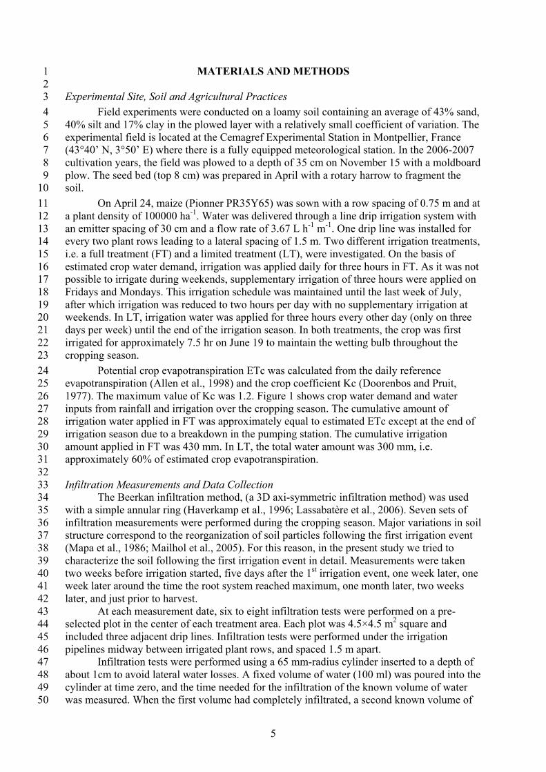
On April 24, maize (Pionner PR35Y65) was sown with a row spacing of 0.75 m and at 11 a plant density of 100000 ha-1. Water was delivered through a line drip irrigation system with 12 an emitter spacing of 30 cm and a flow rate of 3.67 L h-1 m-1. One drip line was installed for 13 every two plant rows leading to a lateral spacing of 1.5 m. Two different irrigation treatments, 14 i.e. a full treatment (FT) and a limited treatment (LT), were investigated. On the basis of 15 estimated crop water demand, irrigation was applied daily for three hours in FT. As it was not 16 possible to irrigate during weekends, supplementary irrigation of three hours were applied on 17 Fridays and Mondays. This irrigation schedule was maintained until the last week of July, 18 after which irrigation was reduced to two hours per day with no supplementary irrigation at 19 weekends. In LT, irrigation water was applied for three hours every other day (only on three 20 days per week) until the end of the irrigation season. In both treatments, the crop was first 21 irrigated for approximately 7.5 hr on June 19 to maintain the wetting bulb throughout the 22 cropping season. 23 Potential crop evapotranspiration ETc was calculated from the daily reference 24 evapotranspiration (Allen et al., 1998) and the crop coefficient Kc (Doorenbos and Pruit, 25 1977). The maximum value of Kc was 1.2. Figure 1 shows crop water demand and water 26 inputs from rainfall and irrigation over the cropping season. The cumulative amount of 27 irrigation water applied in FT was approximately equal to estimated ETc except at the end of 28 irrigation season due to a breakdown in the pumping station. The cumulative irrigation 29 amount applied in FT was 430 mm. In LT, the total water amount was 300 mm, i.e. 30 approximately 60% of estimated crop evapotranspiration. 31 32 Infiltration Measurements and Data Collection 33

The Beerkan infiltration method, (a 3D axi-symmetric infiltration method) was used 34 with a simple annular ring (Haverkamp et al., 1996; Lassabatère et al., 2006). Seven sets of 35 infiltration measurements were performed during the cropping season. Major variations in soil 36 structure correspond to the reorganization of soil particles following the first irrigation event 37 (Mapa et al., 1986; Mailhol et al., 2005). For this reason, in the present study we tried to 38 characterize the soil following the first irrigation event in detail. Measurements were taken 39 two weeks before irrigation started, five days after the 1st irrigation event, one week later, one 40 week later around the time the root system reached maximum, one month later, two weeks 41 later, and just prior to harvest. 42

At each measurement date, six to eight infiltration tests were performed on a pre-43 selected plot in the center of each treatment area. Each plot was 4.5×4.5 m2 square and 44 included three adjacent drip lines. Infiltration tests were performed under the irrigation 45 pipelines midway between irrigated plant rows, and spaced 1.5 m apart. 46

Infiltration tests were performed using a 65 mm-radius cylinder inserted to a depth of 47 about 1cm to avoid lateral water losses. A fixed volume of water (100 ml) was poured into the 48 cylinder at time zero, and the time needed for the infiltration of the known volume of water 49 was measured. When the first volume had completely infiltrated, a second known volume of 50

6

water was added to the cylinder, and the time needed for it to infiltrate was added to the 1 previous time. This procedure was repeated until apparent steady state was reached, i.e. until 2 two consecutive infiltration times were identical, and the cumulative infiltration was then 3 recorded (Lassabatère et al., 2006). In addition, before the infiltration test, a soil sample was 4 extracted in the vicinity of the infiltration ring to determine the initial soil gravimetric water 5 content and particle-size distribution (< 2 mm), the latter being analyzed using the 6 sedimentation method. Another 200 cm3 sample was taken to measure dry bulk density (ρd). 7 Saturated volumetric water content (θs) was calculated as total soil porosity considering the 8 density of the solid particles to be 2.65 g cm-3. 9

10 Soil Hydraulic Characterization and Data Analysis 11

The BEST algorithm (Beerkan Estimation of Soil Transfer parameters) (Lassabatère et 12 al., 2006) was used to determine soil hydraulic properties. This specific algorithm determines 13 characteristic hydraulic curves that take into account the van Genuchten equation for the 14 water retention curve, h(θ), (Eq. 1a) with the Burdine condition (Eq. 1b) and the Brooks and 15 Corey relation (Eq. 2) for hydraulic conductivity curve, K(θ), (Burdine, 1953; Brooks and 16 Corey, 1964; van Genuchten, 1980) : 17

[1a] 18

[1b] 19

[2] 20

where θr and θs are the residual and saturated volumetric water content [L3 L-3], respectively; 21 n and m are shape parameters, and hg is the scale parameter [L] of the water retention curve 22 h(θ), Ks is saturated hydraulic conductivity [L T-1] and η is the shape parameter of the K(θ) 23 relationship. θr is usually very low and was thus considered to be zero. θs was calculated as 24 total soil porosity considering the density of the solid particles to be 2.65 g cm-3. The 25 hydraulic properties were thus represented using five parameters: θs, n, hg, Ks, η. Following 26 Haverkamp et al. (1996), the shape parameters n and η were assumed to mainly depend on 27 soil texture, while θs, hg and Ks were assumed to mainly depend on soil structure. 28

The BEST algorithm estimates the shape parameters from particle-size distribution by 29 classical pedotransfer functions. BEST derives saturated hydraulic conductivity and sorptivity 30 S (L T-0.5) by modeling the 3D infiltrations performed at zero water pressure head (i.e. 31 Beerkan infiltration method). The 3D cumulative infiltration I(t) and the infiltration rate q(t) 32 can be approached by the explicit transient two-term and steady-state equations given by 33 Haverkamp et al. (1994). The reader is referred to the study of Lassabatère et al. (2006) for 34 more details on fitting experimental data on infiltration on analytical expressions that can 35 provide estimations of scale parameters. Lassabatère et al. (2006) also described the main 36 characteristics of the BEST algorithm which is coded with MathCAD 11 (Mathsoft 37 Engineering and Education, 2002). 38

The capillary length (αh) was then estimated from sorptivity (S) and the other 39 hydraulic parameters through (Haverkamp et al., 2006): 40

( ) ss

sp

h

Kc

S

⎥⎥⎦

⎤

⎢⎢⎣

⎡⎟⎟⎠

⎞⎜⎜⎝

⎛−−

=η

θθ

θθ

α0

0

2

1

[3] 41

nm 21−=

( ) η

θθθθθ

⎟⎟⎠

⎞⎜⎜⎝

⎛−−

=rs

r

sKK mn

grs

r

hh

−

⎟⎟

⎠

⎞

⎜⎜

⎝

⎛

⎟⎟⎠

⎞⎜⎜⎝

⎛+=

−− 1θθθθ

7

where θ0 is initial water content and cp is a function of the shape parameters for the van 1 Genuchten (1980) water retention equation (see Haverkamp et al., 2006 and Lassabatère et al., 2 2006). The relationship between the capillary length and the characteristic microscopic pore 3 “radius” i.e., the mean characteristic dimension of hydraulically functional pore, ξm, is known 4 to be: 5

[4] 6 where σ is the surface tension [MT-2], ρw is the density of water [ML-3] and g is the 7 gravitational acceleration [LT-2]. Taking the properties of pure water at 20 °C as appropriate, 8 Equation (4) reduces to 9

[5] 10 where αh and ξm are expressed in mm. 11

Standard statistical analysis was used in this study. In both treatments, the 12 Kolgomorov-Smirnov test was used to check the assumption of normality of the data sets. 13 The effects of time on each soil structure parameter, Ks, αh, ξm and the comparison between 14 the two treatments, FT and LT, were evaluated by analysis of significance using the t-test at 15 0.05 probability level. 16

17 Determining the Horizontal and Vertical Components of the Wetting Front 18

The analytical simulation model developed by Philip (1984) was used to estimate the 19 surface radius (r) and the depth (z) of the wetted soil volume. Because this model relies on 20 assumptions such as the homogeneity of soil hydraulic properties, we used it as indicative 21 rather than perspective. Philip (1984) found that the travel time of the wetting front away 22 from a point source radially and vertically is given for dimensionless time (T), vertical 23 distance (Z) and radial distance (R) as: 24

( )ZZZT ++−= 1ln2

2

[6] 25

and 26

22

exp23

2 −⎥⎦

⎤⎢⎣

⎡+−=

RRRT [7] 27

where 28

316 h

qtTαθπ Δ

= [8a] 29

Zz hα2= [8b] 30 Rr hα2= [8c] 31

where q is the emitter flow rate, t is time, αh is the capillary length and Δθ is the difference 32 between the average volumetric water content in the wetted soil and the initial volumetric 33 water content. 34

hm α

ξ 44.7=

hwm g αρ

σξ =

8

RESULTS AND DISCUSSION 1 2

Soil Hydraulic Properties 3 Combining analysis of particle size distribution with modeling of the 3D infiltration 4

experiments enabled us to fully determine the hydraulic parameters of the water retention and 5 unsaturated hydraulic conductivity curves. Table 1 summarizes the statistical parameters of 6 data sets of physical and hydraulic parameters. 7

The shape parameters of h(θ) and K(θ) varied little over time. This low variability is 8 consistent with the assumption that the shape parameters mainly depend on soil texture 9 (Haverkamp et al., 1996). 10

The Ks, αh, and ξm data sets were consistent with a log normal distribution 11 (Kolgomorov-Smirnov test). Similar results were reported in studies of soil hydraulic 12 properties (Mulla and McBratney 2002). Statistical analysis was thus performed on log-13 transformed values. At almost every measurement date, Ks showed the highest variability with 14 coefficients of variation (CV), ranging from 11% to 43%. The data sets of both ξm and αh 15 showed low CV values ranging from about 14% to 24% over the whole measurement period. 16 This confirms the homogeneity of soil preparation, the precision of the Beerkan infiltration 17 method, and low spatial variability at small scales. 18

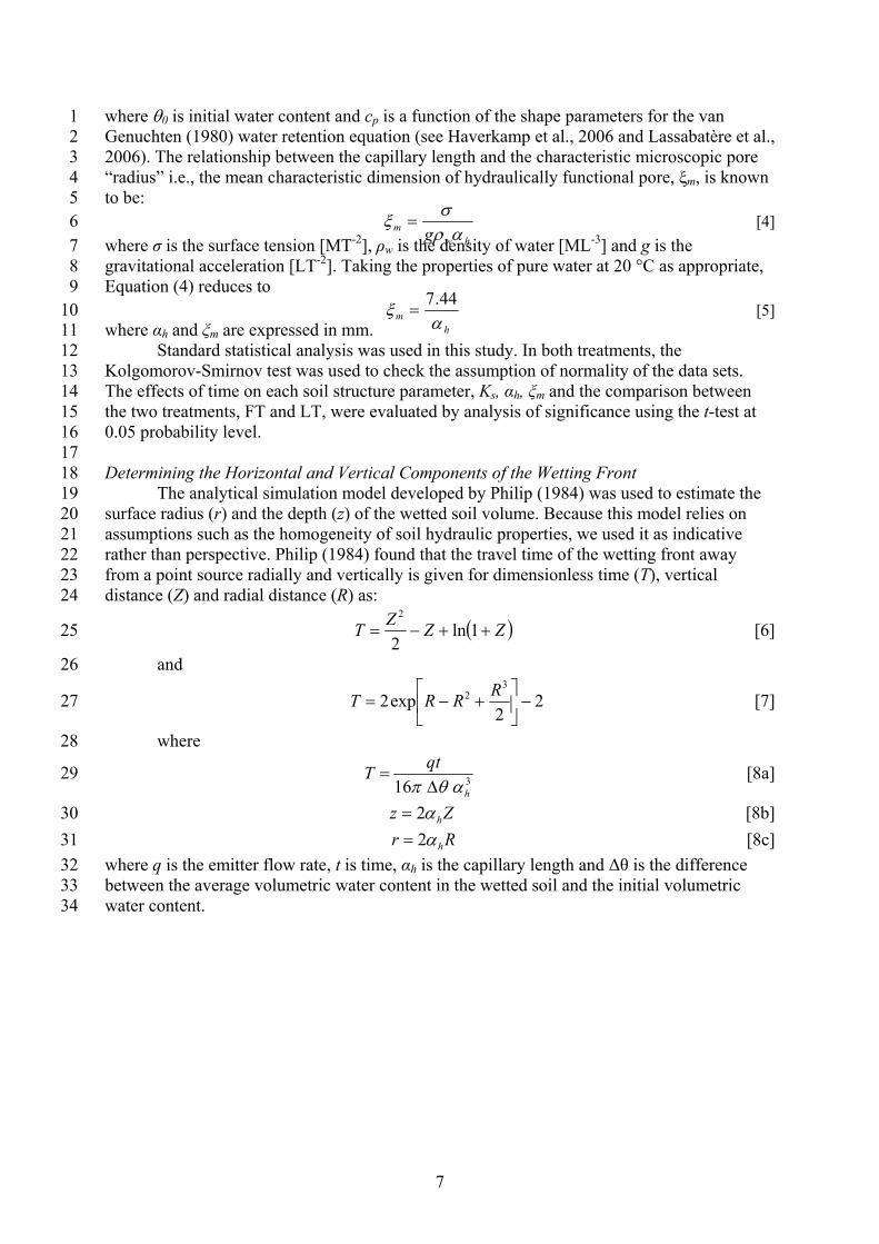
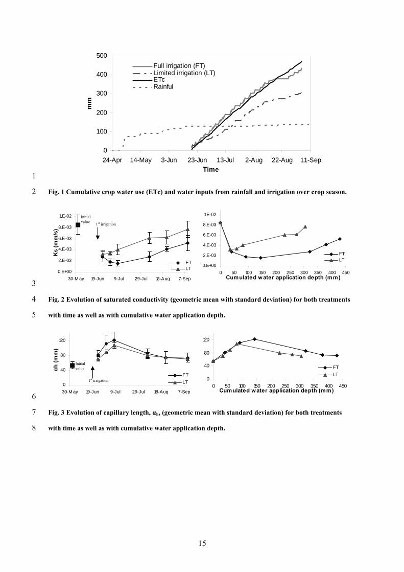
Figures 2, 3 and 4 show the values of Ks , αh, and , ξm obtained during the cropping 19 season in the two treatments, FT and LT, as a function of time and as a function of cumulative 20 water application depth. Each graph can be divided into two separate stages. The first stage 21 lasted from the first irrigation event until July 10 around the time the root system was well 22 established. The second stage lasted until the end of the cropping season. During the 1st stage, 23 hydraulic properties were significantly affected by the first irrigation event (according to the t-24 test) (Table 2). The hydraulic parameters reached their extreme values at the end of this stage. 25 In FT, the mean value of Ks decreased sharply over time and with cumulative water 26 application depth. Its value dropped from 8.5×10-3 mm s-1 to 1.6×10-3 mm s-1 at the end of this 27 stage. It subsequently increased gradually during the second stage to reach a mean value of 28 5.3×10-3 mm s-1 just prior to harvest (Fig. 2 and Table 3). In LT, Ks reached its minimal value 29 (3.3×10-3 mm s-1) only five days after the beginning of the irrigation season. Subsequently, the 30 mean value of Ks did not significantly vary, according to the t-test, for a period of some weeks 31 before rising significantly again to reach 7.7×10-3 mm s-1 at the end of the second stage (Fig. 2 32 and Table 3). 33

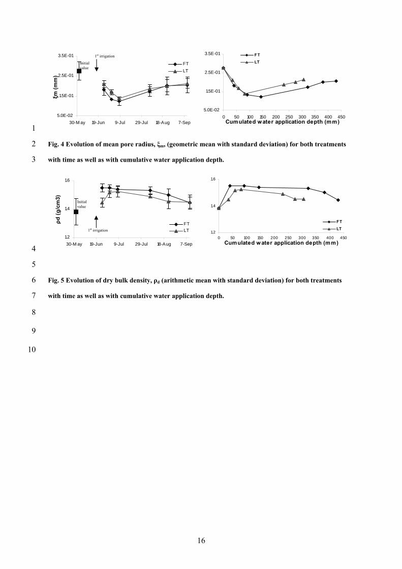
In both FT and LT, ξm decreased from 0.14 mm just before the first irrigation event to 34 about 0.06 mm at the end of the first stage. Subsequently, this parameter gradually increased 35 to reach approximately 0.10 mm at the end of the second stage (Fig. 4 and Table 3). As the 36 mean effective pore radius is inversely proportional to capillary length, the latter displayed 37 inverse behavior with respect to ξm (Fig. 3 and Table 3). It increased significantly from about 38 54 mm before the start of the irrigation season to a maximal value of 120 mm at the end of the 39 first stage. It then decreased gradually to reach a value of about 72 mm just before harvest. 40 The temporal variations in soil hydraulic properties were in agreement with the temporal 41 change in dry bulk density during the cropping season. Dry bulk density showed a significant 42 increase five days after irrigation started, and then stabilized somewhat before starting a 43 downward trend at the end of the second stage (Fig. 5). 44

Temporal variations in soil hydraulic properties were, in general, similar in FT and LT 45 but with different apparent response intensity (Figs 2, 3 and 4). In the second stage, Ks values 46 were significantly higher in LT than in FT, while in the first stage the values did not differ 47 (according to the t-test) (Table 3). No significant differences were found in αh and ξm between 48 the two treatments at each measurement date (t-test) (Table 3). As a function of cumulative 49 water application depth, FT showed that during the irrigation season, the three parameters 50

9

reached their extreme values at the same cumulative water application depth of 144 mm. This 1 value was much higher than that in LT (81 mm) (Figs 2, 3 and 4). 2

In the two treatments, the temporal changes in Ks were generally associated with 3 changes in ξm at all measurement dates and inversely to changes in both ρd and αh. The mean 4 characteristic pore dimension and the capillary length are actual estimates of the capillary 5 component of water transfer into the soil. Thus, the higher ξm, the greater the effect of gravity 6 compared to capillarity, as the infiltration driving force. 7

Temporal changes in the soil hydraulic properties can be commented as follows. At 8 the beginning of the irrigation season, temporal variations in soil hydraulic properties could 9 be due to the “hydraulic” compaction of soil following water application. This is in agreement 10 with the concomitant increase in the dry bulk density (Fig. 5 and Table 1). The volume of 11 water delivered during the first irrigation event and the following frequent irrigations caused 12 restructuration of the fragile structural porosity created by soil preparation operations (Mapa 13 et al., 1986; Angulo-Jaramillo et al., 1997; Cameira et al. 2003). During the second part of the 14 irrigation season, when the irrigation rate decreased due to lower water requirements, the 15 effect of irrigation was overtaken by the effects of wetting and drying cycles associated with 16 the effects of the rooting system. The rooting system could be asymmetric as a result of 17 irrigation with one drip line installed for every two plant rows. Some roots could grow and 18 develop preferentially in the vicinity of emitters, creating new channels or continuity between 19 existing pores. Shirmohammadi and Skaggs (1984) observed that in cropped soils, hydraulic 20 conductivity was much higher than in bare soils due to the effect of the rooting system. 21 Similar results were also reported by Cameira et al. (2003), Iqbal et al. (2005) and Rasse et al. 22 (2000). The latter authors found that the crop rooting system tended to increase water flow 23 resulting in higher Ks values and a larger macroporosity. In addition, as both αh and ξm are 24 characteristic microscopic lengths estimating the capillary component of water transfer, their 25 temporal variations indicated a change in structure of the fine soil fraction. An increase in αh 26 and a decrease in ξm during the first stage indicates that the structural pattern of the fine 27 fraction of soil changed from a poorly connected porous network before irrigation started to a 28 more interconnected network in the middle of irrigation season. The presence of connected 29 pores in that period may be the result of soil biological activity that is locally stimulated by 30 the permanent high humidity of the wetted zone of the soil. White and Sully (1987) linked the 31 higher value of the mean characteristic pore dimension to soil biological activity which is 32 expected to be maximum in the surface soil layer. In addition, during the first stage, the 33 change in these two parameters indicates a decrease in soil porosity leading to an increase in 34 dry bulk density (Fig. 5). The reverse occurred during the second stage, confirmed by an 35 increase in soil porosity at the end of irrigation season, and by a change in structural porosity 36 from an interconnected porous network to a less connected one (Angulo-Jaramillo et al., 37 1997). 38

The processes affecting soil hydraulic properties were similar in the two irrigation 39 treatments. Variations in αh and ξm over time were similar in FT and LT. Although we used 40 two different irrigation schedules i.e., two different water amounts with two different 41 application frequencies, the two microscopic lengths reached their extreme values at the same 42 date i.e., at the end of the first stage, but not at the same cumulated water application depth. In 43 our soil and climatic context, an added cumulated water application depth of from 81 mm to 44 144 mm did not lead to a significant change in the mean values of these two parameters. This 45 indicates that both irrigation management systems play similar roles in the soil matrix. In 46 other words, a change in irrigation management does not appear to adversely influence the 47 fine fraction of the soil. 48

In contrast, Ks values were significantly higher in LT than in FT during the second 49 stage (Fig. 2 and Table 3). In LT, the soil was thus more conductive than in FT. This can be 50

10

attributed to irrigation management. The frequency of water application used in LT (every 1 other day) increased the importance of the alternating daily effects of wetting and drying 2 cycles leading to the formation of the moderate cracks on the soil surface observed with this 3 treatment during measurement campaigns. Thus, we can hypothesize that structural porosity 4 is responsible for the largest water transport fraction (Cameira et al., 2003). This shows that 5 different irrigation management systems mainly affect the larger fraction of pores. This 6 confirms the effects of irrigation, the alternative cycles of wetting and drying, biological 7 activity, root development on soil porosity. 8

The concomitance of extreme values of soil hydraulic properties in the two treatments 9 may be due to the fact that these hydraulic properties are related to the same internal pore 10 geometry. The difference between the two treatments in the cumulated water application 11 depth at which our three hydraulic parameters reached their extreme values can be explained 12 by the different volumes of water applied and by the irrigation schedule that stimulated or not 13 the development of structural porosity in the surface soil layer. 14 15 Effect of Temporal Changes on Simulated Components of the Wetting Front 16

Based on the temporal changes in measured soil hydraulic parameters identified 17 above, three sets of hydraulic properties were used to examine the effects of this phenomenon 18 on the dimensions of the wetted soil volume. The first set represents the fragmented soil 19 before irrigation started, so the initial values of soil hydraulic properties were used. The 20 second set represents the restructuration of the soil some days after irrigation started and the 21 average situation over the irrigation season. The third set represents the extreme situation of 22 “hydraulic” compaction after three weeks of irrigation, that is to say at the 4th measurement 23 date (see Figs. 2, 3 and 4 from June 1 until July 8). The input parameters of the mathematical 24 equations of Philip’s model are (i) two given irrigation periods: t = 12 hr and 24 hr (ii) q = 2 l 25 h-1 as emitter flow rate, (iii) the difference (Δθ = 0.2) between initial water content and mean 26 value of water content of the wetted soil volume which are assumed to be uniform, and (iv) 27 the mean value of capillary length for each hydraulic parameter set. Table 4 shows the width 28 (r) and depth (z) of the wetting pattern computed from Eq. 6, 7 and 8 for the three sets and for 29 the two irrigation periods. For the three parameter sets, it can be seen that the volume of 30 wetted soil and of the water applied to the soil are similar. Results showed that there were 31 differences in the dimensions of the wetting pattern. Initial soil hydraulic properties tended to 32 form slightly vertically elongated bulb. The increase over time in the capillary length, i.e., 33 characteristic of the capillary component of water transfer, led to an increase in the horizontal 34 component of the wetting bulb (about 30%) and to a decrease in its vertical component (about 35 25%) for the two periods of irrigation concerned. In other words, it led to a horizontally 36 elongated bulb. Differences in the dimensions were due only to temporal variability 37 associated with water applications for the two given irrigation periods. 38

11

CONCLUSIONS 1 2 In this study, the behavior of a loamy soil under drip irrigation was analyzed using the 3

Beerkan infiltration method to identify the temporal variability of its hydraulic properties 4 caused by high-frequency irrigation during a maize cropping season. Two different irrigation 5 treatments, a full (FT) and a limited (LT), were investigated. Our results demonstrated that 6 both soil porosity and hydraulic properties varied over time. Soil behavior can be divided into 7 two separate stages. The first stage lasted from the first irrigation event (56 days after sowing 8 of the crop) until the root system was well established (75 days after sowing). During this 9 stage, soil porosity was significantly affected by the first irrigation event, resulting in a 10 decrease in both saturated hydraulic conductivity Ks and in the mean pore effective radius ξm, 11 and in an increase in capillary length αh. These hydraulic parameters reached their extreme 12 values at the end of this stage. This behavior was explained by the “hydraulic” compaction of 13 the surface soil following irrigation. 14

Later in the season, during the second stage, a gradual increase in both Ks and ξm and a 15 gradual decrease in αh were observed in both FT and LT, when the effect of irrigation was 16 overtaken by other phenomena. The latter was put down to the effects of wetting and drying 17 cycles, soil biological activity, and the effect of the root system, which could be asymmetric 18 as a result of irrigation with only one drip line installed for every two plant rows. 19

The processes that affect soil hydraulic properties in the two irrigation treatments were 20 found to be similar. No significant change in mean effective pore radius and in capillary 21 length was observed between FT and LT. However, as a result of daily wetting and drying 22 cycles, which were very marked in LT, the soil was found to be more conductive than in the 23 FT. This shows that different irrigation management systems mainly affect the larger fraction 24 of pores i.e., structural pores. 25

Our work raises questions about the usefulness of taking this phenomenon into 26 account to improve the efficiency of both water and fertilizer under drip irrigation. To answer 27 this question, we studied the impact of temporal changes in soil hydraulic properties on the 28 dimension of the wetting bulb using a simplified modeling approach. Our results 29 demonstrated that there were major differences in the computed width and depth of the wetted 30 bulb when model input parameters measured before and after irrigation were used. An 31 increase in capillary length over time led to the more horizontally elongated bulb. This change 32 can improve the efficiency of both irrigation and fertilization of the root zone and reduce 33 losses of both water and solute due to deep percolation. As a practical result of this study, we 34 recommend fertigation after the restructuration of tilled soil in order to mitigate agro-35 environmental risks and to improve the efficiency of the use of solutes. The temporal changes 36 in soil hydraulic properties identified in our study should be taken into account in future 37 studies when simulating soil water transfer under drip irrigation in order to improve irrigation 38 scheduling practices. 39

40

12

ACKNOWLEDGEMENT 1 2 The AEC of Syria is greatly acknowledged for the Ph.D. scholarship granted to Ibrahim 3 Mubarak. 4

13

REFERENCES 1 2 Allen, R.G., Pereira, L.S., Raes, D. and Smith, M., 1998. Crop evapotranspiration: Guidelines 3

for computing crop requirements. Irrigation and Drainage Paper No. 56, FAO, Rome, 4 Italy, 300pp. 5

Al-Qinna, M.I., Abu-Awwad, A.M., 2001. Wetting patterns under trickle source in arid soils 6 with surface crust. J. Agric. Eng. Res. 80(3): 301-305. 7

Angulo-Jaramillo, R., Moreno, F., Clothier, B.E., Thony, J.L., Vachaud, G., Fernandez-Boy, 8 E. and Cayuela, J.A., 1997. Seasonal variation of hydraulic properties of soils 9 measured using a tension disk infiltrometer. Soil Sci. Soc. Am. J. 61 (1): 27-32. 10

Bresler, E., 1978. Analysis of trickle irrigation with application to design problems. Irrig. Sci. 11 1:03-17. 12

Brooks, R.H. and Corey, C.T., 1964. Hydraulic properties of porous media. Hydrol. Paper 3., 13 Colorado State University, Fort Collins. 14

Burdine, N.T., 1953. Relative permeability calculations from pore size distribution data. Petr. 15 Trans. Am. Inst. Mining Metall. Eng. 198: 71-77. 16

Cameira, M. R., Fernando, R. M. and Pereira, L. S., 2003. Soil macropore dynamics affected 17 by tillage and irrigation for a silty loam alluvial soil in southern Portugal. Soil Tillage 18 Res. 70(2): 131-140. 19

Cook, F.J., Thorburn, P.J., Bristow, K.L., Cote, C.M., 2003. Infiltration from surface and 20 buried point sources: the average wetting water content. Water Resour. Res. 39(12): 21 1364-1376. 22

Doorenbos, J. and Pruitt, W.O., 1977. Guidelines for predicting crop water requirements. 23 Irrigation and Drainage Paper No. 24, 2nd ed., FAO, Rome, 156pp. 24

Haverkamp, R., Ross, P.J., Smetten, K.R.J. and Parlange, J.Y., 1994. Three-dimensional 25 analysis of infiltration from the disc infiltrometer. 2. Physically based infiltration 26 equation. Water Resour. Res. 30: 2931-2935. 27

Haverkamp, R., Arrúe, J. L.,Vandervaere, J.P., Braud, I., Boulet, G., Laurent, J.P., Taha, A., 28 Ross, P. J. and Angulo-Jaramillo, R., 1996. Hydrological and thermal behavior of the 29 vadose zone in the area of Barrax and Tomelloso (Spain): experimental study, analysis 30 and modeling. Project UE, No. EV5C-CT 92 00 90. 31

Haverkamp, R., Debionne, S., Viallet, P., Angulo-Jaramillo, R. and de Condappa, D., 2006. 32 Soil Properties and Moisture Movement in the Unsaturated Zone. In: J. W. Delleur 33 (Editor), The handbook of Groundwater Engineering. CRC, pp. 6.1-6.59. 34

Iqbal, J., Thomasson, J.A., Jenkins, J.N., Owens, P.R. and Whisler, F.D., 2005. Spatial 35 Variability Analysis of Soil Physical Properties of Alluvial Soils. Soil Sci. Soc. Am. J. 36 69: 1338-1350. 37

Lassabatère, L., Angulo-Jaramillo, R., Soria Ugalde, J. M., Cuenca, R., Braud, I. and 38 Haverkamp, R., 2006. Beerkan Estimation of Soil Transfer parameters through 39 infiltration experiments-BEST. Soil Sci. Soc. Am. J. 70: 521-532. 40

Mailhol, JC., Ruelle, P. and Popova, Z., 2005. Simulation of furrow irrigation practices 41 (SOFIP): a field-scale modeling of water management and crop yield for furrow 42 irrigation. Irrig Sci. 24: 37-48. 43

Mapa, R.B., Green, R.E. and Santo, L., 1986. Temporal variability of soil hydraulic-44 properties with wetting and drying subsequent to tillage. Soil Sci. Soc. Am. J. 50(5): 45 1133-1138. 46

Mathsoft Engineering and Eduction, Inc., 2002. MathCad 11, Cambridge. 47 Messing, I. and Jarvis, N., 1993. Temporal variation in the hydraulic conductivity of a tilled 48

clay soil as measured by tension infiltrometers. J. Soil Sci. 44: 11-24. 49

14

Mohanty, B., Ankeny, M., Horton, R. and Kanwar, R., 1996. Spatial analysis of hydraulic 1 conductivity measured using disk infiltrometers. Water Resour. Res. 30: 2489-2498. 2

Mulla, D. J. and McBratney, A. B., 2002. Soil spatial variability. In: M. E. Sumner (Editor), 3 Handbook of Soil Science. CRC press, London, pp. A321-A352. 4

Philip, JR., 1984. Travel times from buried and surface infiltration point sources. Water 5 Resour Res. 20: 990-994 6

Rasse, D.P., Smucker, A.J.M. and Santos, D., 2000. Alfalfa root and shoot mulching effects 7 on soil hydraulic properties and aggregation. Soil Sci. Soc. Am. J. 64: 725-731. 8

Rawlins, S.L., 1973. Principals of managing high frequency irrigation. Soil Sci. Soc. Amer. 9 Proc. 37: 626-629. 10

Revol, P., Clothier, B. E., Mailhol, J.C., Vachaud, G., and Vauclin, M., 1997. Infiltration from 11 a Surface Point Source and Drip Irrigation 2. An Approximate Time-Dependent 12 Solution for Wet-Front Position, Water Resour. Res. 33(8): 1869-1874. 13

Schwartzman, M., Zur, B., 1986. Emitter spacing and geometry of wetted soil volume. J. 14 Irrig. Drain. Eng. 112(3): 242–253. 15

Shirmohammadi, A. and Skaggs, R., 1984. Effect of surface conditions on infiltration for 16 shallow water table soils. Trans. ASAE. 27: 1780-1787. 17

Thorburn, P.J., Cook, F.J., Bristow, K.L., 2003. Soil-dependent wetting from trickle emitters: 18 implications for trickle design and management. Irrig Sci. 22: 121-127. 19

van Genuchten, M.T., 1980. A closed form equation for predicting the hydraulic conductivity 20 of unsaturated soils. Soil Sci. Soc. Am. J. 44: 892-898. 21

Warrick, A.W., 2003. Soil water dynamics. Oxford University Press, 391 pp. 22 White, I. and Sully, M.J., 1987. Macroscopic and microscopic capillary length and time scales 23

from field infiltration. Water Resour. Res. 23: 1514-1522 24 Zur, B., 1996. Wetted soil volume as a design objective in trickle irrigation. Irrig Sci. 16:101-25

105. 26 Zur, B., Ben-Hanan, U., Rimmer, A. and Yardeni, A., 1994. Control of irrigation amounts 27

using velocity and position of wetting front. Irrig Sci. 14: 207-212. 28 29 30 31 32 33 34 35 36 37 38 39 40 41 42 43 44 45 46 47 48 49 50

15

0

100

200

300

400

500

24-Apr 14-May 3-Jun 23-Jun 13-Jul 2-Aug 22-Aug 11-SepTime

mm

Full irrigation (FT)Limited irrigation (LT)ETcRainful

1

Fig. 1 Cumulative crop water use (ETc) and water inputs from rainfall and irrigation over crop season. 2

0.E+00

2.E-03

4.E-03

6.E-03

8.E-03

1.E-02

30-M ay 19-Jun 9-Jul 29-Jul 18-Aug 7-Sep

Ks

(mm

/s)

FTLT

0.E+00

2.E-03

4.E-03

6.E-03

8.E-03

1.E-02

0 50 100 150 200 250 300 350 400 450Cumulated water application depth (mm)

FTLT

3

Fig. 2 Evolution of saturated conductivity (geometric mean with standard deviation) for both treatments 4

with time as well as with cumulative water application depth. 5

0

40

80

120


αh (m

m)

FTLT

0

40

80

120


FTLT

6

Fig. 3 Evolution of capillary length, αh, (geometric mean with standard deviation) for both treatments 7


Initial value 1st irrigation

Initial value

1st irrigation

16

5.0E-02

1.5E-01

2.5E-01

3.5E-01


ξm (m

m)

FTLT

5.0E-02

1.5E-01

2.5E-01

3.5E-01


F T

LT

1

Fig. 4 Evolution of mean pore radius, ξm, (geometric mean with standard deviation) for both treatments 2


1.2

1.4

1.6


ρd (g

/cm

3)

FTLT 1.2

1.4

1.6


F T

LT

4

5

Fig. 5 Evolution of dry bulk density, ρd (arithmetic mean with standard deviation) for both treatments 6


8

9

10

Initial value

1st irrigation

Initial value

1st irrigation

17

Table 1. Statistical parameters of dry bulk density and hydraulic properties for both treatments FT and 1

LT 2

Date Treatment FT ρd gcm-3

θs m3m-3 n m η Ks

mm s-1 αh mm

ξm mm

1st June Mean(8)+ 1.383 0.478 2.201 0.0915 12.93 8.49E-03* 53.9* 0.276*

CV % 6.7 7.3 20.6 18.0 16.3

24th June Mean(8)+ 1.550 0.415 2.210 0.0951 12.52 2.79E-03* 81.2* 0.183*

CV % 1.9 2.4 33.3 15.0 16.4

1st July Mean(6)+ 1.550 0.415 2.210 0.0951 12.52 1.79E-03* 111.1* 0.134*

CV % 1.3 1.9 31.4 21.2 24.2

8th July Mean(8)+ 1.540 0.419 2.210 0.0948 12.54 1.60E-03* 121.0* 0.123*

CV % 1.4 1.9 31.7 18.1 15.6

6th August Mean(6)+ 1.532 0.422 2.210 0.0946 12.57 2.76E-03* 85.6* 0.174*

CV % 1.6 2.0 31.8 14.1 13.8

22thAugust Mean(6)+ 1.500 0.434 2.210 0.0939 12.65 4.17E-03* 73.5* 0.202*

CV % 2.9 4.0 9.1 15.6 14.8

10th September Mean(8)+ 1.445 0.455 2.204 0.0926 12.80 5.26E-03* 72.2* 0.206*

CV % 2.7 3.3 26.1 19.8 19.5

Date Treatment LT ρd gcm-3

θs m3m-3 n m η Ks

mm s-1 αh mm

ξm mm

1st June Mean(8)+ 1.383 0.478 2.201 0.0915 12.93 8.49E-03* 53.9* 0.276*

CV % 6.7 7.3 20.6 18.0 16.3

24th June Mean(8)+ 1.446 0.454 2.206 0.0933 12.72 3.25E-03* 70.5* 0.211*

CV % 2.3 2.7 21.1 8.7 8.4

1st July Mean(6)+ 1.517 0.428 2.210 0.0950 12.53 3.35E-03* 88.4* 0.168*

CV % 2.2 3.0 11.6 7.7 7.6

8th July Mean(8)+ 1.525 0.425 2.210 0.0952 12.51 4.07E-03* 107.1* 0.139*

CV % 2.6 3.3 23.5 6.0 5.8

6th August Mean(6)+ 1.490 0.438 2.210 0.0943 12.60 6.15E-03* 79.7* 0.187*

CV % 0.9 1.0 16.4 11.1 11.0

22thAugust Mean(6)+ 1.452 0.452 2.206 0.0934 12.70 6.25E-03* 74.3* 0.200*

CV % 3.2 3.7 18.6 22.3 22.2

10th September Mean(6)+ 1.451 0.452 2.206 0.0934 12.70 7.72E-03* 69.7* 0.214*

CV % 3.4 4.2 19.1 11.4 11.6 +(Test size) 3 *Geometric mean 4

18

Table 2. Comparison of soil hydraulic properties in each treatment i.e., Full Treatment and Limited 1 Treatment 2

Full treatment Limited treatment Date Ks

mm s-1 αh mm

ξm mm

Ks mm s-1

αh mm

ξm mm

1st June 8.49E-03* 53.9 0.276 8.49E-03 53.9 0.276

24th June 2.79E-03 81.2 0.183 3.25E-03 70.4 0.211

Difference 5.70E-03+ -27.3+ 0.093+ 5.24E-03+ -16.5+ 0.065+

24th June 2.79E-03 81.2 0.183 3.25E-03 70.4 0.211

8th July 1.60E-03 121.0 0.123 4.07E-03 107.1 0.139

Difference 1.19E-03+ -39.8+ 0.060+ -8.21E-04NS -36.6+ 0.072+

8th July 1.60E-03 121.0 0.123 4.07E-03 107.1 0.139

10th September 5.26E-03 72.2 0.206 7.72E-03 69.7 0.214

Difference -3.66E-03+ 48.7+ -0.083+ -3.65E-03+ 37.4+ -0.075+

1st June 8.49E-03 53.9 0.276 8.49E-03 53.9 0.276

10th September 5.26E-03 72.2 0.206 7.72E-03 69.7 0.214

Difference 3.24E-03+ -18.3+ 0.070+ 7.73E-04+ -15.7+ 0.062+

*Geometric mean value. Difference = Date 1 – Date 2 3 + Significance at 0.05 probability level. 4 NS indicates no significant difference. 5 1st June: before irrigation started. 6 24th June: some days after the 1st irrigation event. 7 8th July: rooting system approximately reaches its maximal value 8 10th September: just prior to harvest. 9 10 11 12

19

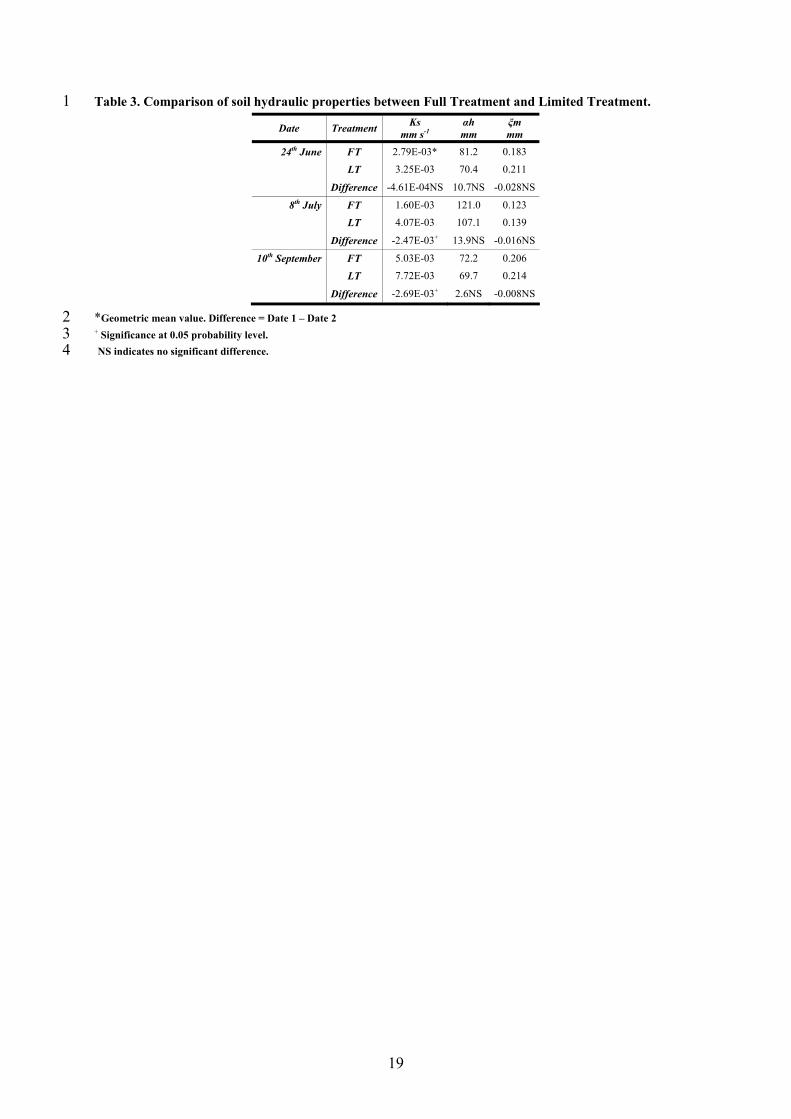
Table 3. Comparison of soil hydraulic properties between Full Treatment and Limited Treatment. 1 Date Treatment Ks

mm s-1 αh mm

ξm mm

24th June FT 2.79E-03* 81.2 0.183

LT 3.25E-03 70.4 0.211

Difference -4.61E-04NS 10.7NS -0.028NS

8th July FT 1.60E-03 121.0 0.123

LT 4.07E-03 107.1 0.139

Difference -2.47E-03+ 13.9NS -0.016NS

10th September FT 5.03E-03 72.2 0.206

LT 7.72E-03 69.7 0.214

Difference -2.69E-03+ 2.6NS -0.008NS

*Geometric mean value. Difference = Date 1 – Date 2 2 + Significance at 0.05 probability level. 3 NS indicates no significant difference. 4

20

Table 4. Comparison of wetting pattern dimensions between different dates for input parameters: q = 2 1 Lh-1 as emitter flow rate, and the difference (Δθ=0.2) between initial water content and mean value of 2 water content of the wetted soil volume supposed uniform 3 4

t=12hr t=24hr

1st June 24th June 8th July 1st June 24th June 8th July The radius of the wetted soil volume, r (cm)= 22.4 25.6 28.5 25.85 30.02 33.85 The depth of the wetted soil volume, z (cm) = 67.3 58.8 52.7 92.5 79.73 70.51

Applied water volume (liter) = qt 24 24 24 48 48 48 Volume of the wetted soil (litre )= qt / Δθ 120 120 120 240 240 240

1st June: before irrigation started. 5 24th June: some days after the 1st irrigation event. 6 8th July: rooting system approximately reaches its maximal value 7 8 9

temporal variability in soil hydraulic properties under

Documents