temporal distributions: the basis for the development of ... · up for co-rotating twin-screw...

1068 POLYMER ENGINEERING AND SCIENCE, JUNE 2001, Vol. 41, No. 6

INTRODUCTION

Mixing is an important component of most poly-mer processing operations. Material processabil-

ity and product properties are highly influenced bymixing quality. Our research is focused on identifyingthe important design and processing parameters en-hancing realization of the mixing process in variousprocessing equipment and defining mixing criteria forprocess optimization and equipment scale-up.

Successful optimization and scale-up is a crucialpart of design and operation of processing equipment.Large mixing devices often require more raw materialand power in order to operate. Thus, it is impracticaland inefficient to have multiple test runs to achieveoptimal operating conditions, and even more so forfinding optimal design parameters. The main discrep-ancy in scale-up stems from the fact that as machinesget larger, the volume per unit length of a mixer in-creases with the square of the scale factor while thesurface areas of equipment only increase linearly.

In the case of internal mixers, some studies (1–4)promote the concept of using the energy input as a

decisive criterion for scale-up. Alternatively, the overallshear strain (1, 5) and the Weber number (6) havealso been used as scale-up criteria for batch mixers.Kawanishi et al. preformed experimental tests on lab-oratory scale Banbury mixers with interchangeablerotors to duplicate rubber blending results of indus-trial scale mixers (7).

In the scale-up of continuous mixers, all variablesof interest are expressed as a power of a characteristicratio, such as the diameter ratio. Traditionally, scale-up strategies have been developed for single-screw ex-truders (8–12), and they are primarily based on con-stant shear rate or constant heat transfer.

Christiano (13) compared different methods of scale-up for co-rotating twin-screw extruders, based onmaintaining constant thermal conduction, constantspecific energy or constant residence time. White andChen (14) performed non-isothermal flow simulationsin a modular co-rotating twin screw extruder and dis-cussed the implications of non-isothermal effects forscale-up. Nakatani proposed an “adiabatic index” crite-ria of keeping the resin temperature unchanged dur-ing scale-up of a twin-screw extruder (15).

In general, not all parameters can be kept the samein scale-up, and choices have to be made. If one con-siders scale-up designed to ensure mixing efficiency,appropriate scale-up criteria for mixing need to be de-fined. Selecting such criteria and applying them incomplex flow geometries pose enormous challenges.

At this point, it is useful to distinguish between thedifferent mixing mechanisms in polymer processing.

Temporal Distributions: The Basis for theDevelopment of Mixing Indexes for

Scale-up of Polymer Processing Equipment

WINSTON WANG and ICA MANAS-ZLOCZOWER*

Department of Macromolecular ScienceCase Western Reserve University

Cleveland, OH 44106

New and better mixing criteria are needed to assess dispersive and distributivemixing efficiency in polymer processing equipment. Such criteria can serve the pur-pose of process optimization and machine scale-up. In this work, the history of flowstrength and shear stresses experienced by a number of particles in a twin-flight,single-screw extruder serve as the basis to produce temporal distributions of theseparameters. In turn, the temporal distributions can be used for developing newmixing indexes for process optimization and scale-up. Using models for dispersionkinetics and experimental data, calculations of agglomerate size distribution andaverage agglomerate size can be used as a dispersive mixing criterion.

*Corresponding author.Ica Manas-ZloczowerDepartment of Macromolecular Science2100 Adelbert Rd. Kent Hale Smith Bldg.Case Western Reserve UniversityCleveland, OH 44106

The mixing mechanism associated with the reductionin size of one component having a cohesive character,within a continuous liquid phase is referred to as dis-persive mixing. The component with a cohesive char-acter may be an agglomerated solid, a liquid dropletor a gas bubble.

In dispersive mixing, agglomerated particles ordroplets held together by interfacial tension must besubjected to mechanical stress in order to reducetheir length scale. Therefore, the most important flowcharacteristics determining dispersive mixing effi-ciency are the flow strength (elongational flow compo-nents) and the magnitudes of shear stresses gener-ated.

Another mixing mechanism, occurring in the ab-sence of a cohesive resistance, is referred to as nondis-persive or extensive mixing. This type of mixing maybe either distributive (rearrangement process) or lami-nar (achieved through deformation).

In distributive mixing, repeated rearrangement ofthe minor component enhances system homogeneity.In continuous mixing processes, composition unifor-mity at the emerging stream is directly related to thematerial residence time distribution. On the otherhand, laminar mixing can be correlated with straindistribution functions.

Lately there has been a great deal of interest in de-velopment of mixing criteria. Many different ap-proaches have been taken by various groups. Yao etal. (16) used a local mixing efficiency criteria based onthe specific rate of stretching of interfacial area to an-alyze distributive mixing in a pin mixing section forsingle screw extruders. Their results are limited to a2D finite difference analysis. Lawal and Kalyon (17)simulated the isothermal flow in single and co-rotat-ing twin screw extruders and used various tools ofdynamics to quantify distributive mixing. Kwon et al.proposed using “deformation characteristics” basedon the Green deformation tensor as a strain and im-plicit mixing measure of screw extrusion processes(18).

Passive tracers have often been used to help evalu-ate mixing in a variety of equipment. These passivetracers are assumed to not affect the flow field andnot interact with each other. Wong and Manas-Zloc-zower (19) studied distributive mixing in internal mix-ers by tracking the motion of passive tracers. Distrib-utive mixing was quantified in terms of the probabilitydensity function of a pairwise correlation function.Avalosse used a similar technique to study mixing ina stirred tank (20). Mackley and Saraiva used kine-matic mixing rates and concentration distributions ofpassive tracers to look at mixing in oscillatory flowwithin baffled tubes (21). Yoshinaga et al. numericallysimulated distributive mixing in a twin screw extruderusing residence time distributions and distribution oflength stretch between tracers (22). Li and Manas-Zloczower (23, 24) and Cheng and Manas-Zloczower(25) have also used tracers to study the dynamics ofthe mixing process and proposed several criteria to

quantify distributive mixing. Shearer and Tzonganakisused reactive polymer tracers as a microscopic probeof the interfacial surface area between two polymermelts and found a nonlinear relationship betweenscrew speed and mixing performance (26).

Residence time distributions have been studied inconjunction with their use in evaluating the distribu-tive mixing in processing equipment. Gao et al. modeledand analyzed the mean residence time and residencetime distribution in a twin-screw extruder (27). Theyand Gasner et al. found a correlation between percentdrag flow and residence time (27, 28). That is, a largerpercentage of drag flow meant the fraction of resi-dence time in the mixing elements decreased, result-ing in poorer mixing quality.

Development of dispersive mixing criteria also posesbig challenges. Gale evaluated mixing by looking atphotomicrographs of samples from extruders, anddiscussed the limitations of using a single-screw ex-truder for dispersive mixing (29). Manas-Zloczowerand Tadmor (30) looked at the distribution of numberof passes over the flights in single screw extruders, asa way to assess dispersive mixing performance. Vainioet al. used the shape of the residence time distribu-tion to evaluate dispersive mixing efficiency (31).

In this work, we focus on defining mixing indexesfor scale-up in reference to the equipment dispersivemixing capability.

DISPERSIVE MIXING CHARACTERIZATION

Studies of droplet breakup in simple shear andpure elongational flows have shown that elongationalflows are more effective, especially in the case of poly-meric blends with high viscosity ratios and low inter-facial tension (32–36). The magnitude of the appliedstresses can also affect the morphology of the result-ing blend. Manas-Zloczower and Feke (37, 38) positedthe same conclusion for the dispersion of solid ag-glomerates in liquids.

As in work previously done by our group (39–41), thedispersive mixing efficiency of a flow field can be char-acterized in terms that account for the elongational flowcontribution and the magnitude of stresses generated.

One simple way to quantify the elongational flowcomponents is to compare the relative magnitudes ofthe rate of deformation, �D

��, and the vorticity, ��

��, ten-

sors. The parameter �old, defined as:

(1)

can be used as a basic measure of the mixing efficiencywhen assessing machine design and/or operating con-ditions. �old is equal to one for pure elongation, 0.5 forsimple shear and zero for pure rotation. Therefore, thecloser the value of �old to one, the better the dispersivemixing efficiency.

A more rigorous method to quantify the elongationalflow components is by employing a flow strength pa-rameter, Sf , that is frame invariant:

�old ��D� �

�D� � � ��

��

Temporal Distributions

POLYMER ENGINEERING AND SCIENCE, JUNE 2001, Vol. 41, No. 6 1069

(2)

where D�° is the Jaumann time derivative of D

�i.e. the

time derivative of D�

with respect to a frame of refer-ence rotating with the same angular velocity as thefluid element. The parameter Sf ranges from zero forpure rotational flow to infinite for pure elongationalflow. A simple shear flow corresponds to a Sf value ofone. For consistency the flow strength parameter canbe normalized according to:

(3)

Like �old, �new is equal to one for pure elongation, 0.5for simple shear and zero for pure rotation. Calcula-tions for �new require the second derivatives of the ve-locities, and is therefore more sensitive to mesh de-sign. A higher uniform mesh density has to be used inorder to reduce numerical errors.

Flow field calculations allow computation of volu-metric distributions of shear stress and the parame-ters �old and, �new. Although useful, especially interms of defining trends, this type of global characteri-zation does not reflect the actual dynamics of the dis-persive mixing process.

Dispersive mixing requires a process of repeatedruptures of the dispersed phase. This is accomplishedby repeated passages in regions of the system wherestress levels above a given threshold value are ap-plied. The number of passages of a fluid elementthrough high stress regions within a given residencetime in the equipment depends on the particularpathline of the fluid element. Different fluid elementsexperience different stress histories and consequentlythe dispersed phase varies in size.

The discussion above suggests that in order to opti-mize mixing and develop valid scale-up criteria, de-tailed knowledge of the mechanisms of flow in theequipment is essential.

DESCRIPTION OF METHOD

In our group we carried out three-dimensional,isothermal flow simulations for various batch andcontinuous mixing equipment (23–25, 30, 40–48).

We first looked at the flow patterns in a twin-flightsingle-screw extruder. A fluid dynamics analysispackage-FIDAP, using the finite element method wasemployed to solve the 3D, isothermal flow of a New-tonian fluid. No slip boundary conditions on thescrew surfaces and barrel walls were used. The oper-ating conditions were selected such that 1 clockwiserevolution of the screw was made per unit time, and apressure difference applied across the inlet and outletsurfaces satisfied the condition of Qp/Qd � �1/2.Here Qd is the drag flow, whereas Qp is the pressureflow in a single-screw extruder. The drag flow compo-nent Qd was obtained in a simulation for which nopressure difference was applied. The normal stress

difference was then adjusted at the inlet and outletplanes until the overall flow rate was equal to one-halfthat of Qd.

FIMESH, a mesh generator that is part of FIDAP,was used to create the computer model.

The equations of continuity and motion for thesteady state, isothermal flow of an incompressibleNewtonian fluid were solved:

(4)

(5)

The Cray T-90 at the Ohio Supercomputer Centerrunning FISOLV was used to solve the field equations.The calculations required 395 user CPU seconds overa total elapsed time of 860 seconds and 11.8 MWordof memory.

We have used an algorithm for particle tracking andfollowed the shear rate/stress histories for a numberof tracers/minor component elements placed randomlyat the inlet of the system. In work previously done byour group (19, 47), an algorithm was developed fortracking massless points that affect neither the flowfield nor other particles. Since the flow field is com-pletely deterministic, the location of the particles canbe found by integrating the velocity vectors:

(6)

where X (t1) is the location of a particle at any time t1,X(t0) is the location of the same particle at initial timet0, and V (t) is the corresponding velocity vector of theparticle. The location of each particle is calculatedevery 0.0001 time step.

We used a coordinate system that rotates with thesame angular velocity as the screw, so that one fi-nite element model can be used for all calculations.Since boundary conditions at the entrance and exit ofthe extruder are determined via a pressure drop, weneed to minimize errors in the flow field. We do this bytracking the particles only in the center portion of theextruder. We place all the initial particles either inpredetermined positions, or randomly in the extruderat an axial position Z�8. This corresponds to the be-ginning of the second pitch, which is the center of themodel, and thereby the most accurate part of the sim-ulation. We then track the particles until they move adistance of �5 in the z direction, at which point theparticles are repositioned one pitch back in the modeland their motion resumes. In this way, we can simu-late an infinitely long extruder via repeated reposition-ing of the particles. The particles are allowed to movefrom Z�3 to Z�13, which in addition to one full pitchincludes a buffer zone that allows particles to changedirections without a lot of extra repositioning. Thenumber of repositions is recorded for each particle sothat the actual distance traveled in the z-direction canbe calculated. Because of the no-slip boundary condi-tions, a particle that runs into, or overshoots, a wall isconsidered to be stuck there and no longer moves.

X 1t1 2 � X 1t0 2 � �t1

t0

V 1t 2 dt

§ # �V V � § V � 3§ # 4§ # V � 0

�new �Sf

1 � Sf

Sf �21tr D

�

2 22

trD�

o 2

Winston Wang and Ica Manas-Zloczower


RESULTS AND DISCUSSION

The radius of the barrel was 4.009623, and the ra-dius of the screw was 3.534884, the flight clearancewas 0.0096, and the flights were 0.44 thick (all di-mensions are in arbitrary but consistent length units.)

The finite element mesh contains 16,200 8-nodebrick fluid elements, and 8340 4-node quadrilateralboundary elements, for a total of 20535 nodes. Figure1 shows a 3-D illustration of the calculation domain,including the mesh of the center cross section. Figure2 shows the complete finite element mesh used.

Figures 3 and 4 show the distribution plots for �oldand �new, respectively, at the center cross section inthe twin-flight single-screw extruder. The two plotsshow similar characteristics, with the majority of thefluid experiencing simple shear flow, and at the root ofthe flights, rotational flow. Figure 5 displays the shearrate/stress (for a Newtonian fluid) distribution at thecenter cross section of the extruder. The darkest re-gions are where the shear rates are over 200 s–1, andthe lightest regions correspond to where the shearrates are under 50 s–1. The flight clearance region ex-hibits the highest magnitude for the stresses gener-ated.

As in our previous work, we have calculated instan-taneous volumetric distributions of shear rate/stressand flow strength parameters (both frame dependentand frame invariant) (41, 45). The results are displayedin Figs. 6–8. The information obtained was used to as-sess, in a global sense, dispersive mixing efficiency.However, this type of global characterization does notreflect the actual dynamics of the mixing process.

To follow the dynamics of the mixing process, wehave used several sets of particles differing only in thenumber of particles in the set and the method bywhich their initial positions are determined. All initialpositions were verified to be inside the mesh design.Figure 9 shows the initial positions for various sets ofparticles differing in number (for all particles the ini-tial axial location corresponds to Z�8). Pathlines for



Fig. 1. 3-D schematic of the calculation domain with themesh of the center cross section displayed.

Fig. 2. Finite element mesh used.

Fig. 3. Distribution plot of �old at the center cross section ofthe twin-flight, single-screw extruder.

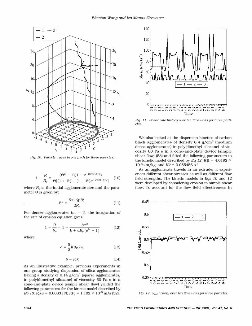
three representative particles traveling for threepitches in the extruder are shown in Fig. 10. The dis-tance from the wall is the essential difference in theinitial positions of particles 1, 2, and 3. Particle 3 islocated closest to the barrel wall, particle 1 is locatedclosest to the screw and particle 2 is located in themiddle of the channel. For the time period tracked (30time units), the particles move in the z direction up to240 units, with the particles in the center of thechannel travelling further than the particles near thewalls. Particle 3 experiences primarily a cross channelmotion, whereas particle 2 moves mainly in the z(axial) direction. Particle 1 is intermediate between thetwo extreme cases.

On each pathline, the exact flow history for the par-ticle (flow strength and shear stress experienced) canbe determined. Figure 11 shows the shear rate historyfor 3 particles initially positioned in a radial array atthe center of the channel for 10 time units (10 revolu-tions of the screw). While particle 3 experiences anearly uniform shear rate of 65 s–1, the true power offlow history shows itself in particle 1, which showsvariations in the shear rate experienced between 60and 110 s–1, and particle 2, which varies in a lowershear rate region of 40–60 s–1. Figures 12 and 13 dis-play the �old and �new history for the same particles.With particle 1, we can see periodic behavior relatedto the particle cycling through different parts of theextruder. The results indicate that the �new oscillateswith larger magnitudes than �old because of the frameinvariant nature of �new.

Particle flow history can also be used to calculatetemporal shear rate and flow strength parameter dis-tributions. Temporal distributions are histogramsdisplaying the flow history of a number of particles in the system, up to a given time. Figures 14 and 15

show the temporal distributions for the flow strengthparameters (�old and �new) calculated for 500 particlesup to a time of 30 units. The temporal distributions ofthe flow strength parameters share the same charac-teristics as the volumetric distributions since the flowtype was relatively uniform throughout the extruder.In Fig. 16, the shear rate temporal distribution for thesame particles is presented.

Particle tracking also allows one to calculate resi-dence time distribution in the equipment. A histogramfor the external residence time distribution for 500 par-ticles after 30 time units in a three-pitch extruder isshown in Fig. 17.



Fig. 4. Distribution plot of �new at the center cross section ofthe twin-flight, single-screw extruder.

Fig. 5. Distribution plot of shear stress at the center crosssection of the twin-flight single-screw extruder.

Fig. 6. Instantaneous volumetric distribution of �old.

PARENT AGGLOMERATE SIZE DISTRIBUTION

Recording the flow history of the particles allowsone to calculate the minor component (agglomerate ordroplet) size distribution at the exit from the extruder.

Previous studies of agglomerate breakup in simpleshear flows (49, 50) have revealed two different disper-sive mechanisms. One mechanism, denoted as ero-sion, is the process of gradual detachment of smallfragments from the outer surface of the agglomerate.The second mechanism, rupture, is characterized byan abrupt breakage of the agglomerate into a fewlarge pieces that can subsequently erode into smallerfragments. Since the erosion mechanism provides thefine fragments that are desirable in typical materialprocessing, we focus on this mechanism and the ki-netics of the erosion process.

Dispersion of agglomerates occurs where hydrody-namic forces acting on a fragment exceed the cohesiveforces at the connection points to its parent cluster.For relatively sparse agglomerates in simple shearflows, erosion kinetics can be described by (51):

(7)

where R is the radius of the agglomerate, t is the time, is a proportionality factor that reflects the fraction ofthe overall hydrodynamic force bearing on the frag-ment, K is a proportionality factor related to the struc-ture of the agglomerate, Fh is the hydrodynamic forceinducing erosion and Fc is the cohesive force resistingfragmentation. The hydrodynamic and cohesive forcescan be written as:

(8)

(9)

with � the fluid viscosity and �̇ the shear rate. Para-meter is a scaling factor that gauges the strength ofthe individual bonds between interacting particleswithin an agglomerate and the exponent m is a mea-sure of packing structure in the agglomerate. m variesfrom 0 for sparse agglomerates to 2 for dense agglom-erates (51).

Integration of the rate of erosion equation for sparseagglomerates (m � 0) gives:

Fc � Rm

Fh �52

��#�R2

�dRdt

� K1Fh � Fc 2 ,



Fig. 7. Instantaneous volumetric distribution of �new. Fig. 8. Instantaneous volumetric distribution of shear rate.

Fig. 9. XY view of initial particle positions.

(10)

where Ro is the initial agglomerate size and the para-meter � is given by:

. (11)

For denser agglomerates (m � 1), the integration ofthe rate of erosion equation gives:

(12)

where,

(13)

(14)

As an illustrative example, previous experiments inour group studying dispersion of silica agglomerateshaving a density of 0.14 g/cm3 (sparse agglomerates)in poly(dimethyl siloxane) of viscosity 60 Pa s in acone-and-plate device (simple shear flow) yielded thefollowing parameters for the kinetic model described byEq 10: Fc/ � 0.00631 N; KFc � 1.102 � 10–5 m/s (52).

We also looked at the dispersion kinetics of carbonblack agglomerates of density 0.4 g/cm3 (mediumdense agglomerates) in poly(dimethyl siloxane) of vis-cosity 60 Pa s in a cone-and-plate device (simpleshear flow) (53) and fitted the following parameters tothe kinetic model described by Eq 12: K � 4.0192 �10–3s m/kg; and Kk � 0.055456 s–1.

As an agglomerate travels in an extruder it experi-ences different shear stresses as well as different flowfield strengths. The kinetic models in Eqs 10 and 12were developed by considering erosion in simple shearflow. To account for the flow field effectiveness in

b � K k

a �52

K��#�,

1 �RRo

� 1 �bebt

b � aRo 1ebt � 1 2

®2 �5��

#R2

o

2Fc.

1 �RRo

�1®2 � 1 2 11 � e�2®KFct>R0 2

® 3 11 � ® 2 � 11 � ® 2e�2®KFc t>R0 4



Fig. 10. Particle traces in one pitch for three particles.

Fig. 11. Shear rate history over ten time units for three parti-cles.

Fig. 12. �old history over ten time units for three particles.

agglomerate dispersion, one may consider a linearflow field as a superposition of pure extension andpure rotation. Bentley and Leal (54) and Kharkharand Ottino (55) have shown that the critical capillarynumber for droplet breakup in different types of flowranging from simple shear to pure elongation dependson the shear rate as well as on a flow strength para-meter. Following their lead, we modify the expressionfor the hydrodynamic force on a spherical agglomeratein the principal strain direction to read:

(15)

where �̇ is the shear rate and � is a flow strengthparameter as defined in Eq 3. Using Eq 15 for thehydrodynamic force will modify the parameters in theerosion kinetics model (Eqs 10 and 12) according to:

(16)

and

(17)

Particle flow histories were used in conjunction withthe erosion kinetic models to calculate the parent ag-glomerate size distribution at the exit from the ex-truder. We have considered 500 agglomerates of initialsize Ro � 1.55 mm and recorded their dispersionalong a three-pitch extruder after 30 revolutions(equivalent to 30 seconds). To calculate the dynamicsof particle size distribution, we account for the reduc-tion in size of the parent agglomerate during eachtime step �t by taking into consideration the actualshear rate and flow strength experienced by the parti-cle during that time step. Also, in the kinetic modelsfor erosion, the initial agglomerate size Ro is adjustedat each time step.

After 30 revolutions, of the 500 initial agglomerates,only 405 have exited the extruder (45 are still in theextruder and 50 hit solid surfaces and were termi-nated). Agglomerate size distributions for the 405 par-ticles exiting the extruder are shown in Fig. 18 for thecase of sparse agglomerates (m � 0) and in Fig. 19 fordenser agglomerates (m � 1). As we would expect, thedenser agglomerates experience less erosion. On aver-age, the agglomerates eroded approximately 77% form � 0 and 37% for m � 1. Also, the standard devia-tion of parent agglomerates (0.0828 for m � 0 and

a � 5�k��#�.

®2 �5��

#Ro

2

Fc

Fh � 5��#�R2



Fig. 13. �new history over ten time units for three particles.Fig. 14. Temporal distribution of �old for 500 particles forthirty time units.

Fig. 15. Temporal distribution of �new for 500 particles forthirty time units.



0.1484 for m � 1) is larger for the denser agglomer-ates, indicating that they are more attuned to varia-tions in the particle flow history.

CONCLUSIONS

Towards the goal of developing new mixing criteriafor process control and equipment scale-up, we havepresented the use of particle tracking as a method ofcapturing the dynamics of the mixing process. Bytracking the motion of particles in the flow field wehave obtained the flow history for each particle (flow

strength and shear stress experienced). Using the flowhistory, we have calculated temporal distributions forthe flow strength and shear stress in a model twin-flight single-screw extruder.

The flow history and temporal distributions forma concrete basis for developing better dispersive mix-ing criteria. The calculation of average agglomeratesize, and agglomerate size distribution illustrate onepossible avenue of developing a new dispersive mixingcriterion for scale-up and optimization of mixing equip-ment.

Fig. 16. Temporal distribution of shear rate for 500 particlesfor thirty time units.

Fig. 17. External residence time distribution calculated using500 particles for thirty time units in a three-pitch extruder.The last bin represents the fraction of particles with a resi-dence time greater than 30 time units. The solid line illus-trates the fraction of particles in the extruder at various times.

Fig. 18. Parent agglomerate size distribution for the 500 par-ticles exiting the three-pitch extruder after thirty time units.Viscosity � 60 Pa s. Model: silica in PDMS (m�0).

Fig. 19. Parent agglomerate size distribution for the 500 par-ticles exiting the three-pitch extruder after thirty time units.Viscosity � 60 Pa s. Model: carbon black in PDMS (m�1).



ACKNOWLEDGMENT

The authors would like to express their gratitude tothe National Science Foundation for supporting thisresearch project under the grant DMI-9812969.

REFERENCES1. P. R. Van Bushkirk, S. B. Turetzky, and P. F. Gunberg,

Rubber Chem. Technol., 48, 577 (1995).2. H. Palmgren, Rubber Chem. Technol., 48, 462 (1975).3. F. S. Meyers and S. W. Newell, Rubber Chem. Technol.,

51, 180 (1978).4. J. Markert, Kautsch. Gummi. Kunstst., 34, 269 (1961).5. J. M. Funt, Plast. Rubber Process., 12, 127 (1977).6. J. Sunder, Kautsch. Gummi. Kunstst., 43, 589 (1990).7. K. Kawanishi, K. Yagii, Y. Obata, and S. Kimura, Int.

Polym. Process., 6, 279–289 (1991).8. J. F. Carley and J. M. McKelvey, Ind. Eng. Chem., 45,

985 (1953).9. J. R. A. Pearson, Plast. Rubber Process, 1, 113 (1976).

10. C. I. Chung, Polym. Eng. Sci., 24, 626 (1984).11. C. Rauwendaal, Polym. Eng. Sci., 27, 1059 (1987).12. C. Rauwendaal, Polymer Extrusion, Hanser (1986).13. J. P. Christiano, SPE ANTEC, 40, 239 (1994).14. J. L. White and Z. Y. Chen, Polym. Eng. Sci., 34, 229

(1994).15. M. Nakatani, Adv. Polym. Technol., 17, 19–22 (1998).16. W. G. Yao, K. Takahashi, and Y. Abe, Int. Polym. Process.,

11, 222–227 (1996).17. A. Lawal and D. M. Kalyon, Polym. Eng. Sci., 35, 1325

(1995).18. T. H. Kwon, J. W. Joo, and S. J. Kim, Polym. Eng. Sci.,

34, 174 (1994).19. T. H. Wong and I. Manas-Zloczower, Int. Polym. Process.,

9, 3–10 (1994).20. T. Avalosse, Macromol. Symp., 112, 91–98 (1996).21. M. R. Mackley and R. Saraiva, Chem. Eng. Sci., 54,

159–170 (1999).22. M. Yoshinaga, et al., Polym. Eng. Sci., 40, 168 (2000).23. T. Li and I. Manas-Zloczower, Int. Polym. Process., 10,

314–320 (1995).24. T. Li and I. Manas-Zloczower, Chem. Eng. Commun.,

139, 223–231 (1995).25. H. F. Cheng and I. Manas-Zloczower, Polym. Eng. Sci.,

38, 926 (1998).26. G. Shearer and C. Tzoganakis, Polym. Eng. Sci., 39,

1584 (1999).27. J. Gao, G. C. Walsh, D. Bigio, R. M. Briber, and M. D.

Wetzel, Polym. Eng. Sci., 40, 227 (2000).28. G. E. Gasner, D. Bigio, C. Marks, F. Magnus, and C.

Kiehl, Polym. Eng. Sci., 39, 286 (1999).

29. M. Gale, Adv. Polym. Technol., 16, 251–262 (1997).30. I. Manas-Zloczower and Z. Tadmor, Adv. Polym. Tech.,

3, 213–221 (1983).31. T. P. Vainio, A. Harlin, and J. V. Seppala, Polym. Eng.

Sci., 35, 225 (1995).32. G. L. Taylor, Proc. Roy. Soc., A146, 501 (1934).33. R. L. Powelln and S. G. Mason, AiChE J., 28, 286

(1962).34. F. D. Rumscheidt and S. G. Mason, J. Coll. Sci., 16, 238

(1961).35. H. P. Grace, Chem. Eng. Commun., 14, 225–277 (1982).36. J. Elmendorp, Polym. Eng. Sci., 26, 418 (1986).37. I. Manas-Zloczower and D. L. Feke, Int. Polym. Process.,

4, 3 (1989).38. I. Manas-Zloczower and D. L. Feke, Int. Polym. Process.,

2, 185 (1987).39. C. H. Yao and I. Manas-Zloczower, Polym. Eng. Sci., 36,

305 (1996).40. C. H. Yao and I. Manas-Zloczower, Int. Polym. Process.,

12, 92–103 (1997).41. C. H. Yao and I. Manas-Zloczower, Polym. Eng. Sci., 38,

936 (1998).42. C. Wang and I. Manas-Zloczower, Intern. Polym. Process

IX, 9, 46–50 (1994).43. C. Wang and I. Manas-Zloczower, Intern. Polym. Process

XI, 115–120 (1996).44. H.-H. Yang and I. Manas-Zloczower, Int. Polym. Process

IX, 291–302 (1994).45. H. Cheng and I. Manas-Zloczower, Int. Polym. Process.,

12, 83–91 (1997).46. H. F. Cheng and I. Manas-Zloczower, Polym. Eng. Sci.,

37, 1082 (1997).47. I. Manas-Zloczower, Rubber Chem. Technol., 67,

504–528 (1994).48. H.-H. Yang and I. Manas-Zloczower, Polym. Eng. Sci.,

32, 1411 (1992).49. S. P. Rwei, I. Manas-Zloczower, and D. L. Feke, Polym.

Eng. Sci., 31, 558 (1991).50. S. P. Rwei, I. Manas-Zloczower, and D. L. Feke, Polym.

Eng. Sci., 30, 701 (1990).51. F. Bohin, D. L. Feke, and I. Manas-Zloczower, Rubber

Chem. Technol., 69, 1–7 (1996).52. F. Bohin, I. Manas-Zloczower, and D. L. Feke, Chem.

Eng. Sci., 51, 5193–5204 (1996).53. Q. Li, D. L. Feke, and I. Manas-Zloczower, Rubber

Chem. Technol., 68, 836–841 (1995).54. B. Bentley and L. Leal, J. Fluid Mech., 167, 241–283

(1986).55. D. V. Khakhar and J. M. Ottino, J. Fluid Mech., 166,

265–285 (1986).

temporal distributions: the basis for the development of ... · up for co-rotating twin-screw...

Documents