Tempered Adversarial Networks

Mehdi S. M. Sajjadi 1 2 Giambattista Parascandolo 1 2 Arash Mehrjou 1 Bernhard Scholkopf 1

AbstractGenerative adversarial networks (GANs) havebeen shown to produce realistic samples fromhigh-dimensional distributions, but training themis considered hard. A possible explanation fortraining instabilities is the inherent imbalance be-tween the networks: While the discriminator istrained directly on both real and fake samples,the generator only has control over the fake sam-ples it produces since the real data distribution isfixed by the choice of a given dataset. We pro-pose a simple modification that gives the genera-tor control over the real samples which leads to atempered learning process for both generator anddiscriminator. The real data distribution passesthrough a lens before being revealed to the dis-criminator, balancing the generator and discrim-inator by gradually revealing more detailed fea-tures necessary to produce high-quality results.The proposed module automatically adjusts thelearning process to the current strength of the net-works, yet is generic and easy to add to any GANvariant. In a number of experiments, we show thatthis can improve quality, stability and/or conver-gence speed across a range of different GAN ar-chitectures (DCGAN, LSGAN, WGAN-GP).

1. IntroductionGenerative Adversarial Networks (GANs) have been intro-duced as the state of the art in generative models (Good-fellow et al., 2014). They have been shown to producesharp and realistic images with fine details (Chen et al.,2016; Denton et al., 2015; Radford et al., 2016; Zhang et al.,2017). The basic setup of GANs is to train a parametric non-linear function, the generator G, which maps samples fromrandom noise drawn from a distribution Z into samples of

1Max Planck Institute for Intelligent Systems, Tubingen,Germany 2Max Planck ETH Center for Learning Systems,Zurich, Switzerland. Correspondence to: Mehdi S. M. Sajjadi<msajjadi.com>.

Proceedings of the 35 th International Conference on MachineLearning, Stockholm, Sweden, PMLR 80, 2018. Copyright 2018by the author(s).

a fake distribution G(Z) which are close in terms of somemeasure to a real world empirical data distribution X . Toachieve this goal, a discriminator D is trained to providefeedback in the form of gradients for the generator. Thisfeedback can be the confidence of a classifier discriminat-ing between real and fake examples (Arjovsky et al., 2017;Goodfellow et al., 2014; Gulrajani et al., 2017; Mao et al.,2017) or an energy defined in terms of a reconstruction lossof an autoencoder (Berthelot et al., 2017; Zhao et al., 2017).

GANs are infamous for being difficult to train and sensitiveto small changes in hyper-parameters (Goodfellow et al.,2016). A typical source of instability is the discriminatorrapidly overpowering the generator which leads to prob-lems such as vanishing gradients or mode collapse. In thiscase, G(X ) and X are too distant from each other and thediscriminator learns to fully distinguish them (Arjovsky &Bottou, 2017). While several GAN variants have been in-troduced to address the problems encountered during train-ing (Arjovsky et al., 2017; Berthelot et al., 2017; Gulrajaniet al., 2017; Zhao et al., 2017), finding stable and more reli-able training procedures for GANs is still an open researchquestion (Lucic et al., 2017).

1.1. Our Contributions

In this work we propose a general and dynamic, yet sim-ple to implement extension to GANs that encourages asmoother training procedure. We introduce a lens moduleLwhich gives the generator control over the real data distribu-tionX before it enters the discriminator. By adding the lensbetween the real data samples and the discriminator, weallow training to self-stabilize by automatically balancinga reconstruction loss with the current performance of thegenerator and discriminator. For instance, a lens could im-plement an image blurring operation which gradually getsreduced during training, thus only requiring the generationof good blurry images at the beginning, which graduallybecome sharper during training. While this analogy fromoptics motivates the term lens, in practice we learn the lensfrom data as explained below.

While the generator in a regular GAN chases a fixed distri-bution X , the proposed lens moves the target distributioncloser to the generated samples G(Z) which leads to a bet-ter optimization behavior.

Tempered Adversarial Networks

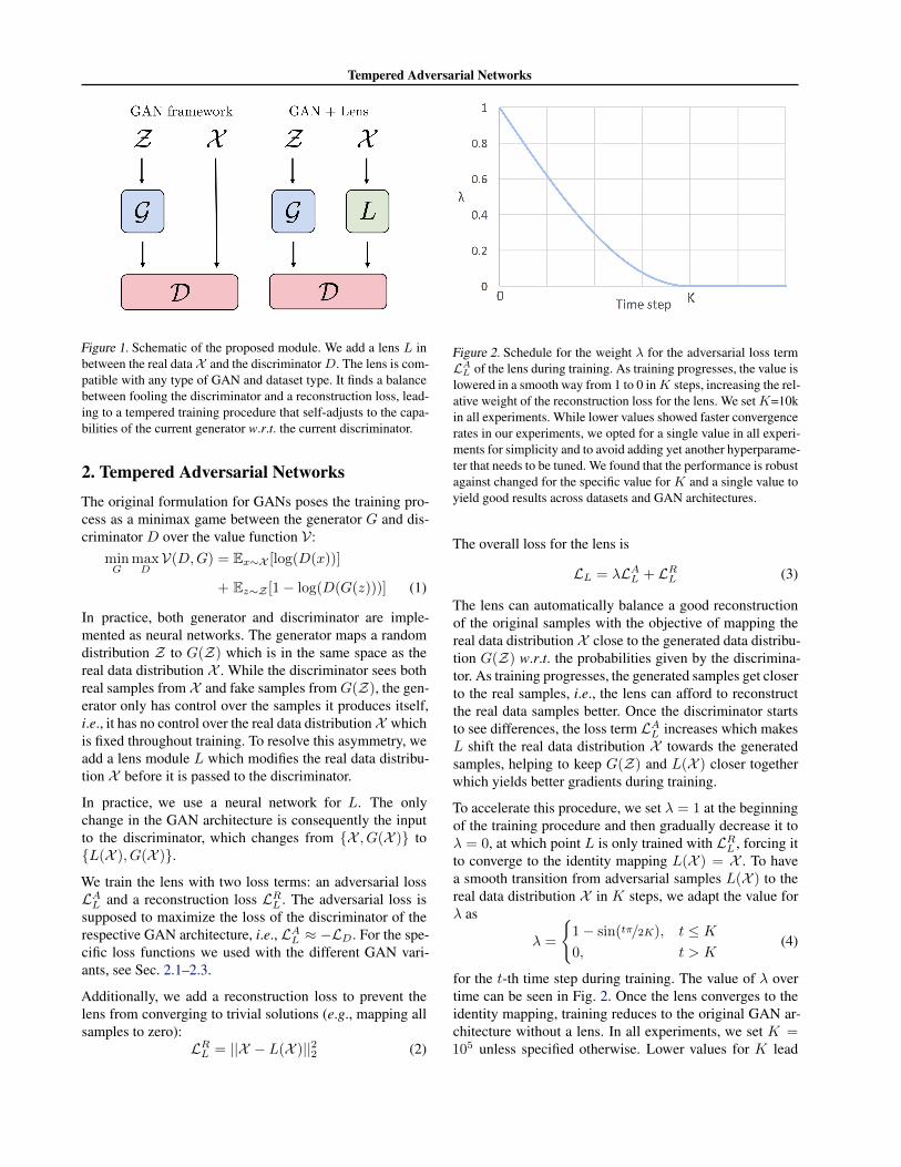
Figure 1. Schematic of the proposed module. We add a lens L inbetween the real data X and the discriminatorD. The lens is com-patible with any type of GAN and dataset type. It finds a balancebetween fooling the discriminator and a reconstruction loss, lead-ing to a tempered training procedure that self-adjusts to the capa-bilities of the current generator w.r.t. the current discriminator.

2. Tempered Adversarial NetworksThe original formulation for GANs poses the training pro-cess as a minimax game between the generator G and dis-criminator D over the value function V:

minG

maxDV(D,G) = Ex∼X [log(D(x))]

+ Ez∼Z [1− log(D(G(z)))] (1)

In practice, both generator and discriminator are imple-mented as neural networks. The generator maps a randomdistribution Z to G(Z) which is in the same space as thereal data distribution X . While the discriminator sees bothreal samples from X and fake samples from G(Z), the gen-erator only has control over the samples it produces itself,i.e., it has no control over the real data distributionX whichis fixed throughout training. To resolve this asymmetry, weadd a lens module L which modifies the real data distribu-tion X before it is passed to the discriminator.

In practice, we use a neural network for L. The onlychange in the GAN architecture is consequently the inputto the discriminator, which changes from {X , G(X )} to{L(X ), G(X )}.We train the lens with two loss terms: an adversarial lossLAL and a reconstruction loss LRL . The adversarial loss issupposed to maximize the loss of the discriminator of therespective GAN architecture, i.e., LAL ≈ −LD. For the spe-cific loss functions we used with the different GAN vari-ants, see Sec. 2.1–2.3.

Additionally, we add a reconstruction loss to prevent thelens from converging to trivial solutions (e.g., mapping allsamples to zero):

LRL = ||X − L(X )||22 (2)

Figure 2. Schedule for the weight λ for the adversarial loss termLA

L of the lens during training. As training progresses, the value islowered in a smooth way from 1 to 0 inK steps, increasing the rel-ative weight of the reconstruction loss for the lens. We setK=10kin all experiments. While lower values showed faster convergencerates in our experiments, we opted for a single value in all experi-ments for simplicity and to avoid adding yet another hyperparame-ter that needs to be tuned. We found that the performance is robustagainst changed for the specific value for K and a single value toyield good results across datasets and GAN architectures.

The overall loss for the lens is

LL = λLAL + LRL (3)

The lens can automatically balance a good reconstructionof the original samples with the objective of mapping thereal data distribution X close to the generated data distribu-tion G(Z) w.r.t. the probabilities given by the discrimina-tor. As training progresses, the generated samples get closerto the real samples, i.e., the lens can afford to reconstructthe real data samples better. Once the discriminator startsto see differences, the loss term LAL increases which makesL shift the real data distribution X towards the generatedsamples, helping to keep G(Z) and L(X ) closer togetherwhich yields better gradients during training.

To accelerate this procedure, we set λ = 1 at the beginningof the training procedure and then gradually decrease it toλ = 0, at which point L is only trained with LRL , forcing itto converge to the identity mapping L(X ) = X . To havea smooth transition from adversarial samples L(X ) to thereal data distribution X in K steps, we adapt the value forλ as

λ =

{1− sin(tπ/2K), t ≤ K0, t > K

(4)

for the t-th time step during training. The value of λ overtime can be seen in Fig. 2. Once the lens converges to theidentity mapping, training reduces to the original GAN ar-chitecture without a lens. In all experiments, we set K =105 unless specified otherwise. Lower values for K lead

Tempered Adversarial Networks

Dense,4C

Reshape,4x4

Tanh

Conv,3

,1/2

ZBa

tchN

orm

Relu

Conv,2

C,1/2

BatchN

orm

Relu

Conv,C

,1/2

BatchN

orm

Relu

Conv,C

,2

Sigmoid

Dense,16C

BatchN

orm

LeakyRe

lu

Conv,2

C,2

BatchN

orm

LeakyRe

lu

Conv,4

C,2

BatchN

orm

LeakyRe

lu

LG

Flatten

LeakyRe

lu

Dense,1

Figure 3. Network architecture of the generator G (top) and dis-criminator D (bottom). The design follows Radford et al. (2016).The strides of the convolutions are 1/2 for upsampling in G and 2for downsampling in D. The kernel size is 4×4 in both networks.The number of parameters can be varied by adjusting C.

to faster convergence, but to avoid introducing a new hy-perparameter that needs to be tuned, and for simplicity, wechoose the same value for all experiments. Note that thischoice is clearly not optimal for all tasks and tuning thevalue can easily lead to even faster convergence and higherquality samples.

2.1. Objectives for classical GAN formulation

In the original work, Goodfellow et al. (2014) use the loss

LG = − log(D(G(Z))) (5)

for the generator, and

LoriginalD = − log(D(X ))− log(1−D(G(Z))) (6)

for the discriminator. The objectives of generator and dis-criminator remain unchanged, though the input of the realdata to D is changed from X to L(X ):LD = − log(D(L(X )))− log(1−D(G(Z))). (7)

The lens is trained against the discriminator with the adver-sarial loss term

LAL = − log(1−D(L(X ))) (8)

which minimizes the output of the discriminator for thelensed data points using the nonsaturating loss.

2.2. Objectives for LSGAN

In LSGAN (Mao et al., 2017), the log-loss is replaced bythe squared distance. This leads to the adversarial loss

LG = ||D(G(Z))− 1||22 (9)

for the generator, and

LD = ||D(G(Z))||22 + ||D(L(X ))− 1||22 (10)

LeakyRe

lu

X

Conv,32

LeakyRe

lu

Conv,3

LeakyRe

lu

Conv,32

Conv,32

…

8x

+

LeakyRe

lu

Conv,32

Conv,32

+ +

Figure 4. Network architecture of the proposed lens that is simi-lar to Sajjadi et al. (2017). The core of the network is composedof 8 residual blocks. To help convergence to identity, we add anadditional residual connection from the input to the output. Allconvolutions have 3×3 kernels and stride 1.

for the discriminator. The lens works against the discrimi-nator with the adversarial loss

LAL = ||D(L(X ))||22 (11)

2.3. Objectives for WGAN-GP

The discriminator or critic in the WGAN-GP variant (Gul-rajani et al., 2017) outputs values that are unbounded, i.e.,there is no sigmoid activation at the after the last dense layerin Fig. 3. The objectives are

LG = −D(G(Z)) (12)

for the generator, and

LD = D(G(Z))−D(L(X )) (13)

for the critic. Again, the lens works against the critic, so weuse the adversarial objective

LAL = D(L(X )) (14)

for the lens for this GAN variant.

2.4. Architecture, Training and Evaluation metrics

The lens can be any function which maps from the usu-ally high-dimensional space of the real data distribution Xto itself. Note that the lens does not need to be injective –in fact, early on during training, mapping several differentpoints to the same data point can be a simple way to de-crease the complexity of the data distribution which willlikely decrease the loss term LAL . Since it is desirable forthe lens to turn into the identity mapping at some point dur-ing training, we have chosen a residual fully convolutionalneural network architecture for the lens, see Fig. 4.

The network architecture and training procedure for thegenerator and discriminator depend on the chosen GANframework. For the experiments with the original GANloss, we use the DCGAN architecture along with its com-mon tweaks (Radford et al., 2016), namely, strided convo-lutions instead of pooling layers, applying batch normal-ization in both networks, using ReLU in the generator and

Tempered Adversarial Networks

leaky ReLU in the discriminator, and Adam (Kingma & Ba,2015) as the optimizer. See Fig. 3 for an overview of thenetworks. LSGAN is trained in the same setting but with-out batchnorm. For the WGAN-GP experiments, we usedthe implementation from Gulrajani (2017) which uses verysimilar models but the RMSProp optimizer (Hinton et al.,2012). We train the lens alongside the generator and dis-criminator and update it once per iteration regardless of theGAN variant. Note that the networks for the DCGAN andLSGAN experiments have intentionally been chosen not tohave a very large number of feature channels to avoid mem-orization on small datasets which is why the results on anabsolute scale are certainly not state of the art. We train us-ing batch sizes of 32 and 64, a learning rate of 10−4 and weinitialize the networks with the Xavier initialization (Glorot& Bengio, 2010).

For quantitative evaluation, previous works have been re-porting the Inception score (Salimans et al., 2016), thoughits accuracy has been questioned (Barratt & Sharma, 2018).Recently, the Frechet Inception Distance (FID) has beenshown to correlate well with the perceived quality of sam-ples, so we follow Heusel et al. (2017) and report FIDscores. Note that a lower FID is better. For computationalreasons, the FID scores are computed on sets of 4096 sam-ples for the DCGAN and LSGAN experiments. While thisis lower than the recommended 10k and should thereforenot be compared directly with other publications, we foundthe sample size to be sufficient to capture relative improve-ments as long as sample sizes are identical. For the WGAN-GP experiments, we used sample sizes of 10k data points.The image size in all experiments is 32×32 pixels with 1color channel for MNIST and 3 color channels for all otherexperiments.

3. Related worksAfter its introduction (Goodfellow et al., 2014), GANs havereceived a lot of attention from the community. There areseveral lines of work to improve the training procedure ofGANs. Radford et al. (2016) proposed heuristic guidelinesfor the design of GAN architectures, e.g., recommendingthe use of strided convolutions and batch normalization(Ioffe & Szegedy, 2015) in both generator and discrimi-nator. Several works follow this trend, e.g., Salimans et al.(2016) propose the use of further methods to stabilize theperformance of GANs including feature matching, histor-ical averaging, minibatch discrimination and one-sided la-bel smoothing (Szegedy et al., 2016). More closely relatedto our work, Arjovsky & Bottou (2017) and Mehrjou et al.(2017) propose adding noise to either both real and fake oronly to the real samples during training with the motivationof increasing the support of the generated and real data dis-tributions which leads to more meaningful gradients. The

amount of noise is reduced manually during training. In ourwork, the lens is not constrained in the mapping that it canapply to balance the training procedure. Furthermore, theeffect of the lens is automatically balanced with a recon-struction term that adjusts the intervention of the lens dy-namically during training depending on the current balancebetween generator and discriminator.

There are several works which approach the problem by us-ing multiple networks instead of one. Denton et al. (2015)propose a Laplacian pyramid of generator-discriminatorpairs for generating images. Zhang et al. (2017) use asimilar approach by using one GAN to produce a low-resolution image and another GAN which produces higher-resolution images conditioned on the output of the low-resolution GAN. Such methods have the drawback that sev-eral GANs need to be trained which increases the num-ber of parameters and introduces a computational bottle-neck. Most recently, Karras et al. (2018) produced convinc-ing high-resolution images of faces by first learning thelow frequencies in images and then progressively growingboth networks to produce higher-resolution images. Whilepromising, all of the methods above are constrained to gen-erating images since the concept of resolution is not easilygeneralizable to other domains.

Another line of research attacks the problem of trainingGANs by changing the loss functions, e.g., Mao et al.(2017) use the least-squares distance loss whereas Arjovskyet al. (2017) approximate the Wasserstein distance whichprovides more stable gradients for the generator. Gulrajaniet al. (2017) improve upon the latter by replacing weightclipping in the discriminator with a gradient penalty whichaccelerates the training procedure considerably.

In the context of training neural networks, Gulcehre et al.(2017) smoothen the objective function by adding noise toactivation functions and then gradually decrease the level ofnoise as training progresses. Bengio et al. (2009) coin theterm curriculum learning where the idea is to present thesamples during training in a specific order that improves thelearning process. Our approach may have a similar effect,but differs in that we present all samples of the originaldataset to the networks, modifying them dynamically in away that stabilizes the learning process.

4. ExperimentsShowing that modifications or additions to GANs lead tobetter results in any way is a delicate topic that has raisedmuch controversy in the community. Most recently, thefindings of Lucic et al. (2017) suggest that with a suffi-cient computational budget, any GAN architecture can beshown to perform at least as well or better than another,if a smaller computational budget is spent on the hyperpa-

Tempered Adversarial Networks

rameter search for the latter. To avoid this fallacy and toprevent choices such as the network architecture or cho-sen hyperparameters to favor one or another method, wefollow common guidelines that are currently in use fortraining GANs and we conduct experiments with three dif-ferent GAN frameworks: the original GAN formulationby Goodfellow et al. (2014); LSGAN, where Mao et al.(2017) replace the log-loss with the least-squares loss; andWGAN-GP, where Gulrajani et al. (2017) minimize the ap-proximated Wasserstein distance between real and gener-ated data distributions and where the training procedure in-cludes a gradient penalty for the discriminator. For the net-work architecture, we follow standard design patterns (seeSec. 2.4). In our experimental section, we do not strive forstate of the art in the end results, but rather we test howmuch of an effect the lens can have on training. We showthat the simple addition of a lens can help improve resultsacross various GAN frameworks. We hope that this insightwill help ongoing efforts to understand and improve thetraining of GANs and other neural network architectures.

In all experiments, the random weights for the initializationof the networks were identical for the GANs with and with-out a lens. All experiments have further been run with atleast 3 different random seeds for the weight initializationto prevent chance from affecting the results.

4.1. Original GAN objective4.1.1. MNIST

We begin with the original GAN variant on the classicalMNIST dataset. To analyze the behavior of the lens, wefirst consider the case of a fixed λ = 1, i.e., the lens hasno direct incentive to become perfect identity. Fig. 5 (top)shows generated and lensed samples at different trainingstages for this architecture. At the beginning of training,the lens scrambles the MNIST digits to look more similarto the generated images. As the generator catches up andproduces digit-like samples, the lens can afford to improvereconstruction. Since the lens acts as a balancing factor be-tween the G and D, this leads to a very stable training pro-cedure. However, even after 10M steps, the reconstructionof the lens still improves, as does the FID score of the gen-erated samples (see FID plot in Fig. 5, bottom left). In com-parison, the GAN without a lens converges much faster tobetter FID scores (Fig. 5, bottom right, green curve).

To accelerate the training procedure, we adapt the weightof λ as explained in Sec. 2. As this forces the lens to turninto a perfect identity mapping at some point during train-ing, the process converges much more quickly and easilysurpasses the quality of the GAN without a lens, yieldingFID scores of 22 (with lens) vs. 42 (without lens). Addi-tional experiments with much larger, heavily fine-tuned ar-chitectures that already show stable training for GANs did

not show better FID after the addition of the lens, indicatingthat the proposed method can stabilize weaker architecturesand lead to more robust GAN training with respect to hy-perparameters.

4.1.2. COLOR MNIST

Since MNIST only has 10 main modes, it is not an adequatetest for the mode collapse problem in GANs. To alleviatethis, a color MNIST variant has been proposed (Srivastavaet al., 2017). Each sample is created by stacking three ran-domly drawn MNIST digits into the red, green and bluechannels of an RGB image which leads to a dataset with1000 modes (assuming 10 modes for MNIST) while stillbeing easy to analyze visually.

As can be seen in Fig. 9, the GAN without a lens firstproduces decent results in all color channels before it col-lapses partially. At this point, only the green color chan-nel looks like MNIST digits while the other two channelsare clearly not from the correct distribution. The FID re-flects this, sometimes even increasing as training proceeds,with values throughout training never getting lower than 50.Adding the lens to the GAN stabilizes training and leads tomuch higher quality samples with an FID of 9 for the bestsamples compared to 53 for the GAN without a lens.

4.2. LSGAN objective4.2.1. MNIST

We found the LSGAN variant to be sensitive to the randomseed for the weight initialization of the networks. LSGANwithout a lens did not train in most cases, with the best runyielding FID scores of 19. With the lens, the networks al-ways trained well, with the worst run producing FID scoresof 16 and the best run giving FID scores of 14.

4.2.2. COLOR MNIST

On the Color MNIST dataset, we found LSGAN to performsimilarly. The best run without a lens yielded FID scoresof 90 and training stalled there due to starved gradients.Adding the lens made the networks produce meaningfulresults in all runs, producing FID scores between 14 and 22from different random initializations.

4.2.3. CELEBA

On the CelebA dataset (Liu et al., 2015), LSGAN was un-stable, with a starving generator early on during trainingdue to a perfect discriminator that did not provide gradi-ents. The best run without a lens yielded an FID score of52. Adding the lens helped the system stabilize and pro-duce meaningful results in all runs, with the best run yield-ing FID scores of 32 and the worst run yielding an FIDof 37. Note that these numbers are comparably high dueto the small model size of the generator and discriminator.The effects of the lens during training are shown in Fig. 10.

Tempered Adversarial Networks

Trainingtim

eGenerated samples G(Z) Lensed samples L(X )

Without lens (FID 42)

Dynamic lens (FID 22)

Real samples X

Figure 5. MNIST digits produced by DCGAN with a lens with fixed λ = 1 (top). The columns show generated and lensed samples.The lens L adds pertubations that make the real data samples look more similar to fake samples. As training progresses, the qualityincreases and the reconstruction of L improves steadily. Ideally, the system would converge to a point where G produces samples thatare indistinguishable from X for a fully trained discriminator – at this point, L would turn into the identity mapping. While training withthe lens is very stable and while the FID was still decreasing when we stopped training, the reconstructions are not perfect even after10M training steps and the FID is still only 60, i.e., it has not yet even reached the performance of DCGAN without a lens after only1M steps (bottom right, green curve). When the value for λ is adapted (see Sec. 2), training is greatly sped up and, the quality of thesamples is substantially higher (FID 22) than for the GAN without a lens (FID 42). The difference is also visible in the results, where theGAN with a lens produces better looking MNIST digits. Note that the FID is initially higher for the GAN with a lens in the bottom right.This is because the FID is always measured against the real samples X , while G is initially trained for the lensed distribution L(X ) thatdiffers from X in the early training stages.

4.3. WGAN-GP

4.3.1. CIFAR10

To test the lens on an entirely different GAN architecture,we also add it to the WGAN-GP framework (Gulrajaniet al., 2017). Wasserstein GANs are generally believed tobe more stable than other GAN variants, making it harderfor tweaks to significantly improve sample quality. Never-

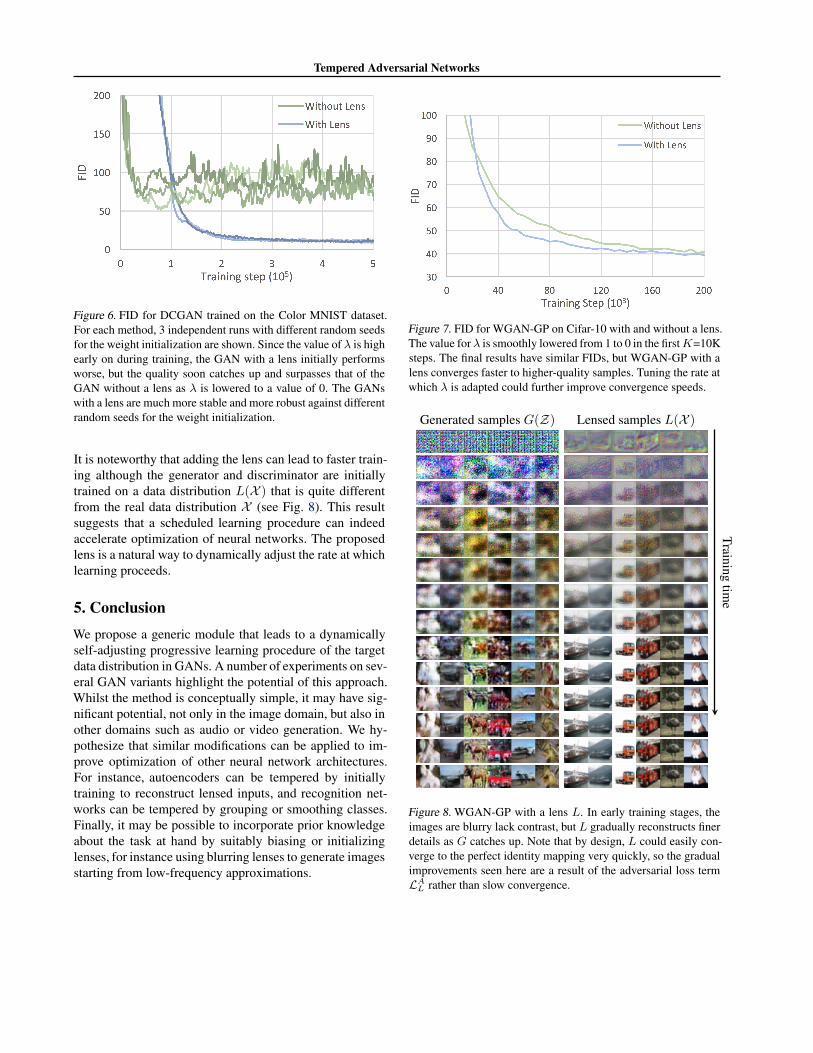
theless, our experiment on the Cifar-10 dataset shows thatthe same lens with the same hyperparameters also workswell with WGAN-GP, yielding higher-quality results asmeasured by the FID score at an earlier training stage. Asseen in Fig. 7, the model with a lens quickly surpasses thequality of the model without a lens and it takes some moretraining time for the GAN without a lens to catch up. Whentrained long enough, both models yield an FID of 39.

Tempered Adversarial Networks

Figure 6. FID for DCGAN trained on the Color MNIST dataset.For each method, 3 independent runs with different random seedsfor the weight initialization are shown. Since the value of λ is highearly on during training, the GAN with a lens initially performsworse, but the quality soon catches up and surpasses that of theGAN without a lens as λ is lowered to a value of 0. The GANswith a lens are much more stable and more robust against differentrandom seeds for the weight initialization.

It is noteworthy that adding the lens can lead to faster train-ing although the generator and discriminator are initiallytrained on a data distribution L(X ) that is quite differentfrom the real data distribution X (see Fig. 8). This resultsuggests that a scheduled learning procedure can indeedaccelerate optimization of neural networks. The proposedlens is a natural way to dynamically adjust the rate at whichlearning proceeds.

5. ConclusionWe propose a generic module that leads to a dynamicallyself-adjusting progressive learning procedure of the targetdata distribution in GANs. A number of experiments on sev-eral GAN variants highlight the potential of this approach.Whilst the method is conceptually simple, it may have sig-nificant potential, not only in the image domain, but also inother domains such as audio or video generation. We hy-pothesize that similar modifications can be applied to im-prove optimization of other neural network architectures.For instance, autoencoders can be tempered by initiallytraining to reconstruct lensed inputs, and recognition net-works can be tempered by grouping or smoothing classes.Finally, it may be possible to incorporate prior knowledgeabout the task at hand by suitably biasing or initializinglenses, for instance using blurring lenses to generate imagesstarting from low-frequency approximations.

Figure 7. FID for WGAN-GP on Cifar-10 with and without a lens.The value forλ is smoothly lowered from 1 to 0 in the firstK=10Ksteps. The final results have similar FIDs, but WGAN-GP with alens converges faster to higher-quality samples. Tuning the rate atwhich λ is adapted could further improve convergence speeds.

Trainingtim

e

Generated samples G(Z) Lensed samples L(X )

Figure 8. WGAN-GP with a lens L. In early training stages, theimages are blurry lack contrast, but L gradually reconstructs finerdetails as G catches up. Note that by design, L could easily con-verge to the perfect identity mapping very quickly, so the gradualimprovements seen here are a result of the adversarial loss termLA

L rather than slow convergence.

Tempered Adversarial Networks

Trainingtim

e

Generated samples G(Z) Lensed samples L(X )

Without lens (t=50k) (FID 47)

Without lens (t=1M) (FID 63)

With lens (FID 8)

Real samples X

Figure 9. Results of DCGAN with a lens L on the Color MNIST dataset (top). The lens gradually improves reconstruction asG producesbetter samples. Once L is a perfect identity function, G adds remaining details and finally produces realistic results (bottom, third row).In comparison, the GAN without a lens only manages to produce good-looking digits in the green color channel and produces noise inthe red and blue channels (bottom, first row, t=50k). As G improves quality in the green channel, the quality in the other two channelsdecreases (bottom, second row, t=1M) which is a commonly encountered instability during GAN training. Several runs with differentrandom seeds for the weight initialization yielded similar results for both architectures, see Fig. 6. Images best viewed in color.

Trainingtim

e

Generated samples G(Z) lensed samples L(X )

← Final samples at the end of training

Figure 10. Generated and lensed samples at various steps during the training process of LSGAN on the CelebA dataset with a lens. Thegenerator produces a large variety of faces since it is not forced to reproduce fine details early during training, making it less prone tothe mode collapse problem.

Tempered Adversarial Networks

ReferencesArjovsky, M. and Bottou, L. Towards principled methods

for training generative adversarial networks. In ICML,2017.

Arjovsky, M., Chintala, S., and Bottou, L. Wasserstein gen-erative adversarial networks. In ICML, 2017.

Barratt, S. and Sharma, R. A note on the inception score.arXiv:1801.01973, 2018.

Bengio, Y., Louradour, J., Collobert, R., and Weston, J. Cur-riculum learning. In ICML, 2009.

Berthelot, D., Schumm, T., and Metz, L. BEGAN:Boundary equilibrium generative adversarial networks.arXiv:1703.10717, 2017.

Chen, X., Duan, Y., Houthooft, R., Schulman, J., Sutskever,I., and Abbeel, P. InfoGAN: Interpretable representationlearning by information maximizing generative adversar-ial nets. In NIPS, 2016.

Denton, E. L., Chintala, S., and Fergus, R. Deep generativeimage models using laplacian pyramid of adversarial net-works. In NIPS, 2015.

Glorot, X. and Bengio, Y. Understanding the difficulty oftraining deep feedforward neural networks. In AISTATS,2010.

Goodfellow, I., Pouget-Abadie, J., Mirza, M., Xu, B.,Warde-Farley, D., Ozair, S., Courville, A., and Bengio, Y.Generative adversarial nets. In NIPS, 2014.

Goodfellow, I., Bengio, Y., and Courville, A. Deep learning.MIT Press, 2016.

Gulcehre, C., Moczulski, M., Visin, F., and Bengio, Y. Mol-lifying networks. ICLR, 2017.

Gulrajani, I. Code for reproducing experimentsin improved training of wasserstein GANs.https://github.com/igul222/improved_wgan_training, 2017. (Latest commit from June 22,2017).

Gulrajani, I., Ahmed, F., Arjovsky, M., Dumoulin, V., andCourville, A. C. Improved training of wasserstein GANs.In NIPS, 2017.

Heusel, M., Ramsauer, H., Unterthiner, T., Nessler, B., andHochreiter, S. GANs trained by a two time-scale updaterule converge to a local nash equilibrium. In NIPS, 2017.

Hinton, G., Srivastava, N., and Swersky, K. Neural net-works for machine learning. overview of mini-batch gra-dient descent, 2012.

Ioffe, S. and Szegedy, C. Batch normalization: Accelerat-ing deep network training by reducing internal covariateshift. In ICML, 2015.

Karras, T., Aila, T., Laine, S., and Lehtinen, J. Progres-sive growing of GANs for improved quality, stability, andvariation. ICLR, 2018.

Kingma, D. and Ba, J. Adam: A method for stochastic op-timization. 2015.

Liu, Z., Luo, P., Wang, X., and Tang, X. Deep learning faceattributes in the wild. In ICCV, 2015.

Lucic, M., Kurach, K., Michalski, M., Gelly, S., and Bous-quet, O. Are GANs created equal? A large-scale study.arXiv:1711.10337, 2017.

Mao, X., Li, Q., Xie, H., Lau, R. Y., Wang, Z., and Smolley,S. P. Least squares generative adversarial networks. InICCV, 2017.

Mehrjou, A., Scholkopf, B., and Saremi, S. Annealed gen-erative adversarial networks. arXiv:1705.07505, 2017.

Radford, A., Metz, L., and Chintala, S. Unsupervised rep-resentation learning with deep convolutional generativeadversarial networks. In ICLR, 2016.

Sajjadi, M. S. M., Scholkopf, B., and Hirsch, M. En-hanceNet: Single image super-resolution through auto-mated texture synthesis. In ICCV, 2017.

Salimans, T., Goodfellow, I., Zaremba, W., Cheung, V., Rad-ford, A., and Chen, X. Improved techniques for trainingGANs. NIPS, 2016.

Srivastava, A., Valkoz, L., Russell, C., Gutmann, M. U., andSutton, C. VEEGAN: Reducing mode collapse in GANsusing implicit variational learning. In NIPS, 2017.

Szegedy, C., Vanhoucke, V., Ioffe, S., Shlens, J., and Wojna,Z. Rethinking the inception architecture for computervision. In CVPR, 2016.

Zhang, H., Xu, T., Li, H., Zhang, S., Huang, X., Wang, X.,and Metaxas, D. StackGAN: Text to photo-realistic im-age synthesis with stacked generative adversarial net-works. In ICCV, 2017.

Zhao, J., Mathieu, M., and LeCun, Y. Energy-based gener-ative adversarial network. ICLR, 2017.