temperature modeling and control in scr-systems for...

Temperature Modeling and

Control in SCR-systems for

Heavy Trucks

Master of Science Thesis

Rikard Dyrsch

Carl Moqvist

Department of Signals and SystemsDivision of Automatic Control, Automation and MechatronicsCHALMERS UNIVERSITY OF TECHNOLOGY

Goteborg, SwedenReport No. EX006/2009

Temperature Modeling and Control in SCR-systems for Heavy Trucks

RIKARD DYRSCHCARL MOQVISTc© RIKARD DYRSCH, CARL MOQVISTSodertalje February 22, 2009

Supervisors: M.Sc. LARS ERICSSONDr. ERIK GEIJER LUNDIN

Examiner: PROF. BO EGARDT

Department of Signals and SystemsChalmers University of TechnologySE-412 96 GoteborgSwedenTelephone + 46 (0)31-772 1000

Abstract

Growing demands on emission reductions in the vehicle industry require the needof better after treatment methods by the truck manufacturers. One method ofNOx reduction is by after treatment of the exhausts with a so called SCR-system;Selective Catalytic Reduction. An SCR-system injects AdBlue, a mixture of ureaand deionized water, into a catalytic reactor in which the urea reduces NOx tonitrogen gas and water.

One problem with AdBlue is the fact that it freezes at −11 ◦C. To prevent it fromfreezing, the components in the SCR-system may be heated, both electrically andwith hot coolant water from the engine. Due to lack of temperature sensors it ishard to know if the AdBlue in all components are liquid and installing more sensorsis very expensive. In this thesis work it is examined if it is possible to estimate thetemperature in the SCR-system with the use of the available temperature sensors.The estimation is done by using physical relations as well as measurement data todetermine unknown parameters. The components that have been dealt with are theAdBlue tank, the pump unit and the suction, pressure and backflow hoses.

The work resulted in a model constructed in Matlab/Simulink, in which it is possibleto simulate the temperatures during different circumstances. The model explainsavailable data well, but more measurements are required to make a thorough vali-dation.

Using the model, different control concepts for the electrically heated pressure hosesare evaluated to see if it is possible to improve the currently used on/off-controlregarding thawing time and energy consumption. Simulations indicate that a feed-back controller is not profitable due to the high cost in a new sensor which can notbe motivated by the energy saving. Instead a proportional open-loop controller issuggested where the knowledge of the hose’s static gain is used to compensate forenvironmental disturbances.

Keywords: SCR, AdBlue, model, Matlab/Simulink, heating control

iii

Sammanfattning

Vaxande emissionskrav inom fordonsindustrin staller krav pa forbattrade metoderfor avgasrening hos dagens lastbilstillverkare. En metod for att rena NOx gaserar genom efterbehandling av avgaserna med hjalp av ett SCR-system; SelectiveCatalytic Reduction. Ett SCR-system injicerar AdBlue, en blandning av urea ochavjoniserat vatten, in i en katalysator dar urean reducerar NOx till att bli kvavgasoch vatten.

Ett problem med AdBlue ar det faktum att det fryser vid −11 ◦C. For att undvikaatt det fryser kan man varma SCR-systemets ingaende komponenter, bade elektrisktoch med hjalp av kylarvatten fran motorn. Pa grund av fa temperatursensorer ardet dock svart att veta om AdBluen i alla komponenter ar flytande och investeringari nya sensorer ar mycket dyra. I foljande examensarbete undersoks darfor om tem-peraturen i SCR-systemet gar att skatta med hjalp av de sensorer som redan finnsatt tillga. Skattningen ar gjord med hjalp av fysikaliska samband tillsammans medmatdata for att bestamma okanda parametrar. De komponenter som undersokts arAdBlue tank och pumpenhet samt sug-, tryck och returslang.

Arbetet resulterade i en modell i Matlab/Simulink, dar man genom enkla simu-leringar kan undersoka vilken temperatur SCR-systemets komponenter har underolika omstandigheter. Modellen beskriver tillganglig data val men fler matningarkravs for att man ska kunna gora en grundlig validering.

Med hjalp av modellen undersoks aven ett antal olika regulatorer for el-varmningenav tryckslangen for att se om den nuvarande on/off regleringen gar att forbattraavseende uppvarmnings tid och energiatgang. Simuleringar indikerar att en ater-kopplad regulator inte ar lonsam da investeringen i den sensor som kravs inte skullebetalas av mangden sparad energi. Istallet foreslas en oppen styrning dar mananvander sig av kunskap om slangens statiska forstarkning for att kompensera motstorningen fran omgivningstemperaturen.

Nyckelord: SCR, AdBlue, modell, Matlab/Simulink, varmereglering

iv

Acknowledgments

First of all we would like to thank Scania CV for the possibility to perform ourMaster of Science thesis within the After Treatment Software group at the R&DDepartment in Sodertalje.

We would also like to thank our supervisors Erik Geijer Lundin and Lars Erikssonat Scania and examiner Bo Egardt at Chalmers University of Technology for all thehelp during the thesis work.

A special thanks to Allesandro Pontecorvi, Peter Loman and Par Karlsson for helpduring measurements, patience lending us equipment all the time and valuable feed-back on the model.

Last, but not least, we would like to thank our families and friends for their support.

Sodertalje, February 22, 2009

RIKARD DYRSCHCARL MOQVIST

v

CONTENTS

NOTATION xi

1 INTRODUCTION 1

1.1 Background . . . . . . . . . . . . . . . . . . . . . . . . . . . . . . . . . . . . . . . . . . . . . . . . . . 1

1.2 Objective . . . . . . . . . . . . . . . . . . . . . . . . . . . . . . . . . . . . . . . . . . . . . . . . . . . . 2

1.3 Requirements . . . . . . . . . . . . . . . . . . . . . . . . . . . . . . . . . . . . . . . . . . . . . . . . . 2

1.4 Method . . . . . . . . . . . . . . . . . . . . . . . . . . . . . . . . . . . . . . . . . . . . . . . . . . . . . . 3

1.5 SCR - Selective Catalytic Reduction . . . . . . . . . . . . . . . . . . . . . . . . . . . . . . 3

1.5.1 General about SCR . . . . . . . . . . . . . . . . . . . . . . . . . . . . . . . . . . . . . . 4

1.5.2 Mobile SCR-systems . . . . . . . . . . . . . . . . . . . . . . . . . . . . . . . . . . . . . 4

1.5.3 The SCR-systems at Scania . . . . . . . . . . . . . . . . . . . . . . . . . . . . . . . 5

1.5.4 Heating Concepts . . . . . . . . . . . . . . . . . . . . . . . . . . . . . . . . . . . . . . . 6

2 MODELING OF THE SCR-SYSTEM 7

2.1 Introduction to Heat Transfer . . . . . . . . . . . . . . . . . . . . . . . . . . . . . . . . . . . . 7

2.1.1 Relation between Temperature and Heat Flow . . . . . . . . . . . . . . . . 7

2.1.2 Modes of Heat Transfer . . . . . . . . . . . . . . . . . . . . . . . . . . . . . . . . . . 8

2.1.3 Overall Heat Transfer Coefficient . . . . . . . . . . . . . . . . . . . . . . . . . . 10

2.2 Parts in the SCR-system . . . . . . . . . . . . . . . . . . . . . . . . . . . . . . . . . . . . . . . . 10

2.2.1 Properties of AdBlue . . . . . . . . . . . . . . . . . . . . . . . . . . . . . . . . . . . . 11

2.2.2 Hose Models . . . . . . . . . . . . . . . . . . . . . . . . . . . . . . . . . . . . . . . . . . . 12

2.2.3 AdBlue Tank Model . . . . . . . . . . . . . . . . . . . . . . . . . . . . . . . . . . . . . 15

2.2.4 Pump Unit Model . . . . . . . . . . . . . . . . . . . . . . . . . . . . . . . . . . . . . . . 16

2.2.5 Nonlinearities . . . . . . . . . . . . . . . . . . . . . . . . . . . . . . . . . . . . . . . . . . . 18

2.3 Calculations of Initial Conditions . . . . . . . . . . . . . . . . . . . . . . . . . . . . . . . . . 18

vii

viii CONTENTS

3 PARAMETER TUNING DATA 20

3.1 Measurements on a Complete SCR-system . . . . . . . . . . . . . . . . . . . . . . . . . 20

3.1.1 Preparations . . . . . . . . . . . . . . . . . . . . . . . . . . . . . . . . . . . . . . . . . . . 20

3.1.2 Performed Tests . . . . . . . . . . . . . . . . . . . . . . . . . . . . . . . . . . . . . . . . 23

3.2 Complementary Tests . . . . . . . . . . . . . . . . . . . . . . . . . . . . . . . . . . . . . . . . . . 27

3.2.1 Electrically Heated Pressure Hoses . . . . . . . . . . . . . . . . . . . . . . . . . 27

3.2.2 Pump 1 & 2 . . . . . . . . . . . . . . . . . . . . . . . . . . . . . . . . . . . . . . . . . . . 28

4 RESULTS OF THE TEMPERATUREESTIMATION 30

4.1 Hose Temperature Estimation . . . . . . . . . . . . . . . . . . . . . . . . . . . . . . . . . . . 31

4.1.1 Coolant Heated Hoses . . . . . . . . . . . . . . . . . . . . . . . . . . . . . . . . . . . 31

4.1.2 Electrically Heated Hoses . . . . . . . . . . . . . . . . . . . . . . . . . . . . . . . . . 31

4.1.3 Analysis of the Hose Temperature Estimation . . . . . . . . . . . . . . . . 32

4.2 AdBlue Tank Temperature Estimation . . . . . . . . . . . . . . . . . . . . . . . . . . . . . 32

4.2.1 Analysis of the AdBlue Tank Temperature Estimation . . . . . . . . . 34

4.3 Pump Unit Temperature Estimation . . . . . . . . . . . . . . . . . . . . . . . . . . . . . . 34

5 CONTROL OF ELECTRICAL HEATING 35

5.1 The Electrically Heated Hose on State Space Form . . . . . . . . . . . . . . . . . . 35

5.2 Properties of the Different Hoses . . . . . . . . . . . . . . . . . . . . . . . . . . . . . . . . . 36

5.3 Control Design . . . . . . . . . . . . . . . . . . . . . . . . . . . . . . . . . . . . . . . . . . . . . . . . 38

5.3.1 On/off Open-loop Control . . . . . . . . . . . . . . . . . . . . . . . . . . . . . . . . 38

5.3.2 Proportional Open-loop Control . . . . . . . . . . . . . . . . . . . . . . . . . . . 38

5.3.3 Feedback Control . . . . . . . . . . . . . . . . . . . . . . . . . . . . . . . . . . . . . . . 40

5.4 Results and Analysis of the Control . . . . . . . . . . . . . . . . . . . . . . . . . . . . . . . 43

6 DISCUSSION 45

6.1 Temperature Estimation . . . . . . . . . . . . . . . . . . . . . . . . . . . . . . . . . . . . . . . . 45

CONTENTS ix

6.2 Control Methods . . . . . . . . . . . . . . . . . . . . . . . . . . . . . . . . . . . . . . . . . . . . . . 46

6.3 Simulink Model Applications . . . . . . . . . . . . . . . . . . . . . . . . . . . . . . . . . . . . 47

6.4 Implementation in the Truck Control Unit . . . . . . . . . . . . . . . . . . . . . . . . . 47

7 CONCLUSIONS 48

APPENDIX 51

A Simulink Implementation 51

A.1 Hose Model . . . . . . . . . . . . . . . . . . . . . . . . . . . . . . . . . . . . . . . . . . . . . . . . . . 51

A.2 Tank Model . . . . . . . . . . . . . . . . . . . . . . . . . . . . . . . . . . . . . . . . . . . . . . . . . . 52

A.3 Pump Model . . . . . . . . . . . . . . . . . . . . . . . . . . . . . . . . . . . . . . . . . . . . . . . . . 52

A.4 Complete SCR-model . . . . . . . . . . . . . . . . . . . . . . . . . . . . . . . . . . . . . . . . . . 52

A.5 User-Friendly Simulation Environment . . . . . . . . . . . . . . . . . . . . . . . . . . . . . 52

NOTATION

The following notations are used throughout the report.

Capital Letters

A area [m2]Cp specific heat capacity [J/kgK]L length [m]P power [W ]Q heat flow rate [W ]T temperature [K]U overall heat transfer coefficient [W/m2K]W energy [J ]

Lower-case Letters

e energy flux [W/m2]h heat transfer coefficient [W/m2K]l level [%]m mass [kg]q heat flux [W/m2]t time [s]x thickness [m]

Greek Letters

λ thermal conductivity [W/mK]ρ density [kg/m3]

Symbols

� diameter [m]

xi

xii Chapter 0 Notation

Subscripts

Ab Adbluec coolantco coldcond conductionconv convectioncr cross sectional areaelec electricalenv environmenth hosel liquidn non-blackp pump units solidt tanksa surface areaseg segmentset setpointtot totalwa warm

1 INTRODUCTION

In this chapter a background to the work and specified requirements are given to-gether with objective and methods used. A general introduction to SCR-systems isalso given.

1.1 Background

Constantly growing demands on emission control require more efficient ways of tak-ing care of the emissions. During combustion in a diesel engine the main emissionsare hydrocarbons, carbon dioxide, nitrogen oxides, sulphur oxides and particles(Nilsson 2006). The goal for Scania CV AB is of course to be able to limit theamount of emissions that the vehicles produce but this is also regulated by rulesin the different continents. In Europe the current regulation is called Euro IV andis valid until October 2008 when Euro V will be in effect. Euro V and even moreEuro VI, which will be valid from 2012, focuses in particular on nitrogen oxides, seeFigure 1.1 (Nilsson 2006). To be able to meet these demands, improvements on thecurrent exhaust treatment is required.

Figure 1.1. Allowed NOx in the European emission standards.

A common way of solving this in the heavy truck industry is by after treatment ofthe exhausts. Since many years both heavy trucks and personal cars use catalyticconverters to reduce the emissions. These are placed in the exhaust pipe and areused to convert the raw emissions into less harmful substances.

One specific type of catalytic converter is SCR; Selective Catalytic Reduction. Byadding ammonia into the exhausts, nitrogen oxides can be turned into water andnitrogen gas which are not harmful to the environment. Since ammonia is considered

1

2 Chapter 1 Introduction

poisonous and has an unpleasant smell the chemical compound urea is used instead.On the market this is sold as AdBlue which is a combination of urea and deionisedwater.

One drawback with AdBlue is the fact that its freezing-point is at a temperatureof −11 ◦C which makes it difficult to handle in a cold environment. AdBlue itselfis not damaged by the freezing and the SCR-system is also constructed to stand it,but the crystallization of the liquid makes it impossible to inject the frozen AdBlueinto the exhausts. To prevent freezing and for thawing of a frozen system, heatingis required. The heating can be based either on electrical energy, hot coolant waterfrom the engine or both.

When AdBlue is frozen in the system it is important that it can be thawed as fastas possible to get the system started again. But since heating of the SCR-system isenergy demanding there is a trade-off between fast thawing of the AdBlue and anenergy-saving method of doing it.

To control the heating of the SCR-system in an energy effective way, informationabout the temperature in specific points of the system is needed. Due to lack ofsensors a physichal model has to be used to estimate the temperature in importantparts of the system.

1.2 Objective

The primary objective with the project is to construct a model in Matlab/Simulinkthat describes the temperature in different parts of an SCR-system used at Sca-nia. The model should be constructed in such a way that even those with limitedknowledge about Matlab/Simulink are able to interpret the results and configureparameters. The model should also be on a general form, so that it is easy to adjustit to different physical setups and heating concepts. The model should focus ontemperatures in different parts of the system under cold circumstances, i.e. whenthe AdBlue is frozen or is under risk of freezing.

The secondary objective is to present a concept of how the system should be thawedin an efficient way with respect to both time and power usage when the AdBlueis frozen. This includes a study of the current used method and to develop andexamine new methods that could be used instead.

1.3 Requirements

Some requirements were set up to be able to evaluate the work after the project wasfinished.

1.4 Method 3

Model requirements:

• The temperature in all relevant parts of the SCR-system must be estimated.

• There must be a Simulink model presented for each SCR-system of interest,e.g. systems from different manufacturers.

• Properties of different components in the system such as hose dimensions andAdBlue tank volume shall be adjustable.

• Coolant water heating and electrical heating must be available in the model.

• The model shall be built such that people with only basic skills in Matlab canuse it and interpret the results.

• The model must be well documented.

Control requirements:

• Evaluate the current control method and give suggestions of possible improve-ments regarding thawing time and energy consumptions.

1.4 Method

The model is based on physical relations. However, to get the model to behaveaccording to the real system, measurement data is used for parameter adjust-ments. The model is implemented in Matlab/Simulink which is widely used both atChalmers University of Technology and at Scania CV AB.

Using knowledge from the modeling, alternative control methods were developed.These were then compared to each other and with today’s thawing method withrespect to thawing time and energy consumption.

1.5 SCR - Selective Catalytic Reduction

Of the currently available techniques for reduction of NOx in diesel engines, selectivecatalytic reduction, or SCR, is one of the most powerful. The technology was firstused in the 1970’s but then only in power plants and other stationary installations.After further development of the technology it was in the 1990’s adapted to mobileapplications, first in the marine industry and as late as in 2004 the first commercialheavy truck with SCR was available on the market. (Ericson 2007)

This section will give a brief introduction to SCR in heavy trucks in general and atScania in particular.


1.5.1 General about SCR

The SCR technology is based on a chemical reductant that is applied in the exhaustflow upstream of the catalyst. The active chemical reagent is ammonia, NH3, butas mentioned before this is, due to its unpleasant properties, used in the chemicalcompound known as urea, (NH2)2CO. Injected in the hot exhausts the urea resolvesinto ammonia and carbon dioxide as

(NH2)2CO + H2O → NH3 + CO2 (1.1)

In the catalyst the ammonia reacts with nitrogen oxide and forms nitrogen gas andwater as (Engman 2006)

NH3 + NOx → N2 + H2O (1.2)

In addition to the fact that AdBlue freezes at −11 ◦C there are a few difficulties withthe SCR system. First of all it is under many conditions not possible to reach 100%NOx reduction. Partly this is due to the fact that the catalyst has much slowerdynamics than the engine; the catalyst typically requires several minutes to get tochemical equilibrium, compared to a few milliseconds for the diesel engine. Also thecatalyst has a relatively small temperature window in which a high conversion ratecan be achieved, below 200 ◦C and above 450 − 500 ◦C the conversion is severelydecreased. Another important factor that has to be taken into account is the socalled ammonia-slip. The ammonia-slip is a measurement of how much ammoniathat passes the catalyst without being converted. This is unwanted because of theunpleasant smell and also because there are laws that regulate the amount of allowedammonia-slip. (Ericson 2007)

1.5.2 Mobile SCR-systems

When used in mobile applications the main components of the SCR-system are theAdBlue tank, pumping unit, dosing unit, SCR catalyst and a control unit. The flowof AdBlue and information (e.g. sensors signals) is illustrated in Figure 1.2.

The SCR-system has sensors for temperature and level in the AdBlue tank andexhaust temperature before the catalyst. There is also a NOx sensor placed afterthe catalyst. Information about the current working point (torque and rpm) of theengine is also of use and available for the SCR-system.

Based on measurements of the temperature of the exhausts as well as informationabout the current working point of the engine, the amount of produced NOx andthe potential to reduce this can be calculated by the electric control unit, ECU.The ECU then calculates the amount of AdBlue that should be injected and sendsthis information to the dosing unit. To further increase the performance the ECUcan correct the amount of injected AdBlue by feedback of the difference betweenmeasured NOx after the catalyst and the setpoint of allowed NOx .

1.5 SCR - Selective Catalytic Reduction 5

Figure 1.2. Flow of AdBlue and information in an SCR-system. The greenarrows are flow of AdBlue, the solid black arrows control signals and the dottedarrows are sensor signals. c© Christian Kunkel, Scania CV

1.5.3 The SCR-systems at Scania

Two SCR-systems have been dealt with during this project, from now on referredto as System 1 and System 2. These systems work in principle rather similarlybut differ at some points. The main components are the AdBlue tank, pump unit,dosing unit, suction hose, backflow hose and pressure hose. The main differencebetween the systems lies in the way the temperature in the dosing unit is controlled,see Figure 1.3. Due to the placement of the unit, in connection with the hot exhaustpipe prior to the silencer, both cooling and heating of the dosing unit have to betaken into account.

In System 1 coolant from the engine is used to cool the dosing unit. This flow isuncontrollable and pumped to the dosing unit as long as the engine is running. Theheating of the dosing unit relies on the hot temperature from the silencer. Thereforeboth the suction and backflow hoses are connected to the pump unit and redundantliquid is directly pumped back to the tank.

In System 2 another method is used for the temperature control in the dosing unit.Instead of using coolant water from the engine, System 2 takes advantage of thecooling effect from the AdBlue liquid by having the backflow hose connected to thedosing unit instead of to the pump.


(a) System 1

(b) System 2

Figure 1.3. The heating and cooling concepts of System 1 and System 2.

Due to the placement of the dosing units at the exhaust silencer these are automat-ically heated and therefore not taken into consideration in this project.

1.5.4 Heating Concepts

Two methods are available to thaw frozen AdBlue, and heat up AdBlue which isliable of freezing; electrical heating and coolant water heating. In this project thecoolant from the engine is used to heat the AdBlue tank and the pump unit whilethere are both coolant water heated and electrically heated hoses used. The coolantis controlled with a water valve which can only be in the states on and off and theelectrical heating can be controlled by a PWM-signal.

2 MODELING OF THE SCR-SYSTEM

The model of the SCR-system is based on both physical properties and measurementdata and mainly structured as described in the three phases of modeling (Ljung andGlad 1994). According to this method the system is first divided into smaller sub-systems and the degree of approximations are determined. The different subsystemsare then examined further and the basic equations are formulated. In the last phasethe equations are structured and suited for simulations.

In this chapter an introduction to heat transfer gives the fundamental equations andrelations that the modeling is based on. A detailed description of how each part ofthe SCR-system is modeled then follows.

2.1 Introduction to Heat Transfer

Heat transfer between different media or within a medium is basically dependenton two things; temperature and heat flow. Temperature is a measure of the storedenergy and heat flow is a measurement of the movement of thermal energy fromone place to another. There are several material properties that affect temperatureand heat flow. The most important of these includes specific heat capacity, thermalconductivity and material density. For more advanced calculations, fluid velocitiesand viscosity must also be taken into account but that will not be dealt with in thisreport. (Lienhard IV and Lienhard V 2008)

2.1.1 Relation between Temperature and Heat Flow

The laws governing heat transfer are typically relationships between the quantitiestemperature T and heat flow rate Q. Heating an object means that temperatureincreases as a function of the energy flow into the object. This gives the relation

Q(t) = Cd

dtT (t) (2.1)

where C is the thermal capacity. The temperature as function of the heat flow rateis then

T (t) =1

C

∫ t

0

Q(s)ds + T (0) (2.2)

In some cases the thermal capacity C depends on the temperature and the temper-ature function is then replaced by a nonlinear expression. (Ljung and Glad 1994)

7

8 Chapter 2 Modeling of the SCR-system

2.1.2 Modes of Heat Transfer

There are three different types of heat transfer that can occur in a heat transfer pro-cess, either by themselves or in combinations; conduction, convection and radiation.

Conduction

Conduction occurs when thermal energy flows from one region of higher temperatureto a region with lower temperature due to molecular contact in a medium or betweenmediums in direct physical contact. Different materials have widely different thermalconductivities which are due to the big variations in molecular structures. Generallyconduction increases with density because of the decreased distances between themolecules.

The fundamental law of heat conduction, Fourier’s law, states that heat flow througha material is proportional to the negative temperature gradient and the area throughwhich the heat is flowing. If the constant of proportionality is called λ, then Fourier’slaw can be stated as:

qcond = −λdT

dx(2.3)

where qcond is the heat flux, λ is called thermal conductivity , T is temperature andx is the direction in which heat flows.

In one dimensional heat conduction problems Fourier’s law can be written in simplescalar form as

qcond = λ∆T

L(2.4)

where L is the thickness of the material in which heat flows and ∆T is the temper-ature difference. The variables qcond and ∆T are written as positive quantities, i.ewhen expressing the heat flux on this form one must remember that heat alwaysflows from hotter to colder regions.

The total heat flow rate Qcond in a material is the heat flux multiplied by the areaA, through which the heat flows. This gives the relationship

Qcond = qcondA = λA∆T

L(2.5)

(Lienhard IV and Lienhard V 2008)

Convection

Unlike heat transfer by conduction where the heat flows only by direct molecularcontact, heat transfer by convection involves moving and mixing of small portionsof a fluid or gas. Since convection involves motion of matter, convection can not

2.1 Introduction to Heat Transfer 9

occur at all in solids. There are two types of convection; natural and forced convec-tion. Natural convection occurs when the motion and mixing is caused by densityvariations resulting in different temperatures inside the fluid. Forced convection iscaused by an outside force e.g. a fan or a pump.

Heat transfer by convection involves no single property of the heat transfer medium;instead properties like fluid velocity, fluid viscosity, and surface roughness all affectthe mechanism of convection. Therefore convection is usually treated empiricallybecause of all the varying factors.

The basic relationship for convective heat transfer is

qconv = h∆T (2.6)

where qconv is the heat flux, h is called the convective heat transfer coefficient and∆T is the temperature difference between two mediums. In the same way as forconduction the total heat flow, Qconv, can be stated as

Qconv = hA∆T (2.7)

where A is the area in which the two mediums are in contact. (Lienhard IV andLienhard V 2008)

Radiation

Thermal radiation is the temperature flow from an object caused by electromagneticradiation from the object’s surface. Any object with temperature different fromabsolute zero will emit thermal radiation, which is generated when the kinetic energywithin atoms is converted to electromagnetic radiation.

According to Stefan-Boltzmann’s law, the energy flux e radiated from a non-blackbody is

e(T ) = εσT 4 (2.8)

where σ = 5, 670400× 10−8 [W/m2K4] is called the Stefan-Boltzmann constant andε, 0 < ε ≤ 1, is the emittance for the body, i.e the proportion of energy flux radiatedfrom a non-black body in comparison to a black body with the same temperature.For black bodies, which are perfect emitters and absorbers, ε = 1.

The heat transfer due to radiation from this body is then

Q = eA = εσAT 4 (2.9)

where A is the area of body. (Lienhard IV and Lienhard V 2008)

Since the heat transfer is proportional to the temperature to the power of four,the heat transfer due to radiation is significant for warm bodies. For colder bodieshowever the emitted energy from radiation can often be neglected compared toconvection and conduction. Therefore heat transfer by radiation will not be treatedfurther in this report.


2.1.3 Overall Heat Transfer Coefficient

In many practical applications a heat transfer process involves a combination of bothconduction and convection. To deal with this the overall heat transfer coefficientis commonly used. This can be thought of as the general conductance to the heattransfer rate. A relevant example is a tank containing liquid and surrounded byair, see Figure 2.1. The heat transfer through the tank wall is mainly affected

Figure 2.1. Heat flow through a tank wall with thickness x and thermal con-ductivity λ.

by three things; convection between the liquid and the wall characterized by h1,the heat transfer in the wall determined by the wall thickness x and the thermalconductivity λ and the convection by air on the outside of the tank, represented byh2. The overall heat transfer coefficient U can then be stated as

U =1

1h1

+ xλ

+ 1h2

(2.10)

The total heat transfer rate, Qtot, is then

Qtot = UAsa,t(Tl − Tair) (2.11)

where Asa,t is the tank surface area, Tl the bulk temperature of the liquid and Tair

the temperature of the surrounding air. (Lienhard IV and Lienhard V 2008)

2.2 Parts in the SCR-system

The three main parts of the system that are modeled are the hoses, the AdBlue tankand the AdBlue pump. All system parts have one thing in common, AdBlue, whichproperties are described first. A detailed description of how the different parts aremodeled then follows and here the different heat flows are explained. A descriptionof the Simulink implementation is also presented.

2.2 Parts in the SCR-system 11

−20 0 20 40 60 80 1001040

1060

1080

1100

1120

Temperature Adblue [°C]

Den

sity

Adb

lue

[kg/

m3 ]

Figure 2.2. Change of density as function of temperature.

2.2.1 Properties of AdBlue

AdBlue, the mixture between urea and deionised water, is chosen at its eutecticcomposition which means the point with the lowest freezing temperature. For Abluethis is a composition of 32,5% urea and 67,5% deionised water and a freezing pointat −11 ◦C. (BASF Aktiengesellschaft 2005)

The specific heat capacity Cp for AdBlue varies with the temperature. This changehowever is very small within each phase. The big difference occurs at the phasechange between liquid and solid why two mean values can be used to approximatethe specific heat capacity within the phases: (aus der Wiesche 2007)

Cp,l ≈ 3.4 [J/kgK]

Cp,s ≈ 1.6 [J/kgK]

A larger temperature dependence can be seen for the density ρAb of liquid AdBlue.This dependence is shown in Figure 2.2 and described by

ρAb,l = 1100.01− 0.428345T − 1.62819 ∗ 10−3T 2 (2.12)

where T is the temperature in ◦C (BASF Aktiengesellschaft 2005). The smalldensity change in the solid phase can be neglected, assuming that the behaviour offrozen Adblue is similar to that of frozen water. The expansion coefficient for ice isa factor ten smaller than for water. (Nordling and Osterman 2004)

Another important variable used for thermal calculations is the conductivity, λAb,which also differs depending on the phase, liquid or solid: (aus der Wiesche 2007)

λAb,l = 0.57 [W/mK]

λAb,s = 0.75 [W/mK]

In addition to the variable changes dependent of the AdBlue phase mentioned aboveis a property called enthalpy of fusion. This is the amount of energy requiredto create disorder among the structured molecules in the solid state and causesthe temperature around the melting point to be constant until the enthalpy of


melting is reached. The same behaviour can be seen in the opposite direction, incrystallization of liquid, which then is the amount of energy required to order themolecules (Sandler 2006). The specific melting heat of AdBlue is 270 [J/g] (BASFAktiengesellschaft 2005).

2.2.2 Hose Models

For both System 1 and System 2 there are three hoses present; suction hose, backflowhose and pressure hose. There are several different types of hoses and thereforemodels over all, at the time, available types of hoses are made. The concept ofmodeling hoses is independent of the type of hoses used, even though the physicalproperties of the hoses differ in some aspects.

To be able to estimate the temperature in several parts of the hose, it is divided inton segments with a specific length L. In this project n = 4 has been used. The modelof the hose is then based on the different heat flows into and out from each segmentas described in Figure 2.3. For simplicity the heat flow along the hose material isneglected since the effect from this is assumed to be very small.

Figure 2.3. A segment of the hose and the direction of heat flow defined.

Because the thickness of the hose wall is large compared to the diameter of theAdBlue channel it must be taken into account when designing the model. Themodel is based on the assumption that the heating does not directly affect theAdBlue in the hose, instead the heating whether it is electric or coolant acts to heatthe hose itself which in turn heats the AdBlue.


The heat flow into each segment Qin and the flow out from each segment Qout is theconductive heat flow that depends on the cross-sectional area Acr, the length of thesegment L, the thermal conductivity of AdBlue λAb, and the temperature differencebetween the segments. Let TAb,seg be the temperature of the AdBlue in currentsegment and TAb,seg−1, TAb,seg+1 the temperatures in the previous and next segmentrespectively. With this notation, the heat flow rate in and out of the segment canbe described as in Equation (2.5) which gives

Qin =λAb

LAcr(TAb,seg−1 − TAb,seg) (2.13)

Qout =λAb

LAcr(TAb,seg − TAb,seg+1) (2.14)

In the first segment TAb,seg−1 is the temperature from the previous component backto the AdBlue tank which can be denoted T0. In the same way TAb,seg+1 in the lastsegment is the temperature in the next component.

The convective heat flow between the hose wall and the environment, Qenv, is cal-culated as in Equation (2.7) which gives

Qenv = henvAsa(Th,seg − Tenv) (2.15)

where henv is the convective heat transfer coefficient between the hose surface andthe environment, Asa is the outer surface area of the segment, Th,seg is the hosematerial temperature of the segment and Tenv the ambient temperature.

As discussed earlier, two methods are available for external heating of the hoses;electrical heating and coolant water heating. Depending on the method used theproperties of the hose is changed regarding material and number of channels. Thehose with electrical heating has a single channel with a metal wire winded aroundit conducting heat to the AdBlue homogenously. The calculation of Qelec is thensimply based on the power into the segment as

Qelec =Ptot

n(2.16)

where Ptot is the total electric power delivered to the hose.

The coolant heated hoses has two channels as shown in Figure 2.4. In this case, theheat flow from the coolant to the hose material can be described as

Qc = hcAsa,c(Tc − Th,seg) (2.17)

where hc is the convective heat transfer coefficient between the coolant and the innersurface area of the coolant channel in the segment, Asa,c. Tc is the temperature ofthe coolant from the engine. For simplification the coolant water temperature isconsidered constant through the entire hose.

The hose is in turn heating the AdBlue as

Qh = hAbAsa,Ab(Th,seg − TAb,seg) (2.18)


Figure 2.4. Cross section of a double channel hose. The large channel is forcoolant water and the small one for AdBlue.

where hAb is the heat transfer coefficient between AdBlue and the inner surface areaof the AdBlue channel Asa,Ab. Here, depending on the phase of the AdBlue in thehose, hAb can either describe the conductive heat transfer between the hose and solidAdBlue or, when the AdBlue is liquid, the convective heat transfer between the hoseand the AdBlue.

Th,seg is, with signs defined as in Figure 2.3, determined by

Th,seg(t) =1

mhCp,h

(Qadded(t)−Qh(t)−Qenv(t)) (2.19)

where mh is the mass of the hose segment material and Cp,h is its specific heatcapacity. Qadded can either be Qelec as in Equation (2.16) or Qc as in Equation (2.17).

There is also a heat transfer caused by the physical flow of AdBlue liquid, Qflow,calculated as

Qflow = kflow(TAb,seg−1 − TAb,seg) (2.20)

where kflow [W/K] is determined by measurement data. In reality kflow is dependenton the flow speed of the liquid. However, as long as the flow is turned on it isrelatively constant through the system why the variations to flow speed can beneglected. There are ways to describe this flow more accurately, but since theflow is not relevant for the main problem in this project the above simplification isconsidered a good enough approximation.

By adding the heat flows in Equation (2.13)-(2.14) and Equation (2.18)-(2.20) thetemperature of the AdBlue in each segment can be determined by

TAb,seg(t) =1

mAbCp,Ab

(Qin(t)−Qout(t) + Qh(t) + Qflow(t)) (2.21)

where mAb is the mass of AdBlue in the segment.

Tuning Parameters

In addition to kflow there are for both the coolant heated and the electrically heatedhoses parameters that can not be acquired from tables or datasheets. These param-


eters are the ones that are adjusted to get the right behavior of the model. For theelectrically heated hoses the convective heat transfer coefficient hAb is unknown andfor the coolant heated hoses the convective heat transfer coefficients hAb and hc areunknown. Both of the hose types also have the unknown parameter henv.

2.2.3 AdBlue Tank Model

Due to the fact that there is a temperature sensor in the AdBlue tank this part ofthe SCR-system is not necessary to model to be able to control the temperature.However, there is still interest in having a model for the tank as well. The modelcould be used to get a hint of how the coolant pipes should be configured to geta sufficiently fast heating. Another scenario is that the temperature sensor is mal-functioning. This can be more easily detected if there is a model that can predictthe tank temperature based on the ambient and coolant temperature together withthe time the truck has been turned on.

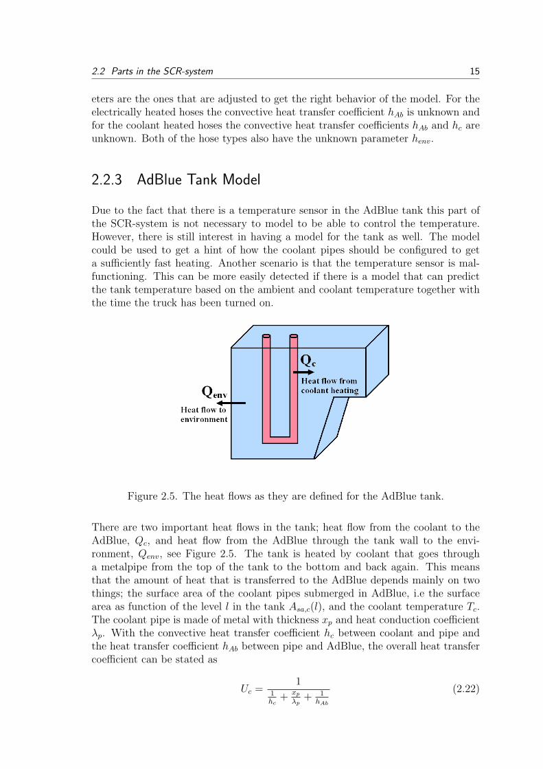
Figure 2.5. The heat flows as they are defined for the AdBlue tank.

There are two important heat flows in the tank; heat flow from the coolant to theAdBlue, Qc, and heat flow from the AdBlue through the tank wall to the envi-ronment, Qenv, see Figure 2.5. The tank is heated by coolant that goes througha metalpipe from the top of the tank to the bottom and back again. This meansthat the amount of heat that is transferred to the AdBlue depends mainly on twothings; the surface area of the coolant pipes submerged in AdBlue, i.e the surfacearea as function of the level l in the tank Asa,c(l), and the coolant temperature Tc.The coolant pipe is made of metal with thickness xp and heat conduction coefficientλp. With the convective heat transfer coefficient hc between coolant and pipe andthe heat transfer coefficient hAb between pipe and AdBlue, the overall heat transfercoefficient can be stated as

Uc =1

1hc

+ xp

λp+ 1

hAb

(2.22)


The total heat transfer rate from coolant to AdBlue is then

Qc = UcAsa,c(l)(Tc − Tt) (2.23)

where Tt is the tank temperature.

The other significant heat flow is the one from AdBlue to the surrounding air. Thisdepends on the tank material and the wall thickness. If the tank material hasthe heat conduction coefficient λt and thickness xt, the convective heat transfercoefficient between the tank wall and the environment is henv, and the heat transfercoefficient between the AdBlue and the tank wall is hAb then the overall heat transfercoefficient can be stated as Equation (2.10) which gives

Uenv =1

1hAb

+ xt

λt+ 1

henv

(2.24)

Assuming that the area of the tank which on the inside is covered by AdBlue isAt(l), the total heat flow to the surrounding air is

Qenv = UenvAt(l)(Tt − Tenv) (2.25)

where Tenv is the ambient air temperature.

The temperature in the tank is then given by

Tt(t) =1

mAb,tCp,Ab

(Qc(t)−Qenv(t)) (2.26)

where mAb,t is the mass of the AdBlue in the tank.

Unlike for the hoses, the coolant water temperature is not considered constant duringthe flow through the tank. An easy way of describing the temperature after the tankis

Tc,out = Tc − Lclkt(Tc − Tt) (2.27)

where Lc is the length of the coolant pipe, l is the AdBlue level [%] and kt is aconstant that specifies the heat loss per meter [m−1].

Tuning parameters

The unknown parameters for the tank that will be used for tuning are the threeconvective heat transfer coefficients hc, hAb and henv. The coolant water heat lossconstant kt is also considered unknown.

2.2.4 Pump Unit Model

The two pumps’ complex shape and construction makes it hard to accurately modelthem using physical relations. However, simple relations can be stated and by


looking at measurement data, parameters can be adjusted to make the model behaveaccordingly. As for the hoses it is assumed that the ambient temperature as well asthe coolant heating acts on the pump unit which in turn affects the temperature ofthe AdBlue within the pump. There are then four different heat flows that are ofimportance; the heat flow due to heating from the coolant water Qc, the heat flowto the environment Qenv, the heat flow between the pump unit and the AdBlue Qp

and the heat flow caused by physical flow of the AdBlue liquid Qflow.

Figure 2.6. Heat flows in to and out from the pump unit.

With directions as shown in Figure 2.6 the heat flows out from and in to the pumpunit can be stated as

Qenv = henvAp,out(Tp − Tenv) (2.28)

andQc = hcAp,in(Tc − Tp) (2.29)

where Ap,out and Ap,in is the outer and inner area of the pumps.

The temperature of the pump unit is in turn affecting the AdBlue temperature as

Qp = hpAsa,Ab(Tp − TAb) (2.30)

where Asa,Ab is the total inner surface area of the AdBlue channels.

The pump temperature can now be determined by

Tp(t) =1

mpCp,p

(Qc(t)−Qenv(t)−Qp(t)) (2.31)

where mp is the mass of the pump unit and Cp,p its specific heat capacity.

As with the hoses, the AdBlue temperature is also dependent on the physical flowof liquid described by

Qflow = kflow(TAb,in − TAb) (2.32)


where TAb,in is the temperature of the AdBlue flowing in to the pump. This, togetherwith Qp gives the AdBlue temperature in the pump unit as

Tp,Ab(t) =1

mAbCp,Ab

(Qp(t) + Qflow(t)) (2.33)

Tuning Parameters

Due to the complex shape of the pump units, both concerning the outside surfacearea and the area of the coolant and AdBlue channels on the inside, these areconsidered unknown. The products henvAp,out, hcAp,in, hpAsa,Ab in Equation (2.28),(2.29) and (2.30) will then be considered to be tuning parameters.

2.2.5 Nonlinearities

Due to the fact that AdBlue has different properties depending on its phase, anumber of nonlinearities have to be dealt with in the model. These nonlinearitieshave in common that they all appear in the zone of phase change between liquidand solid AdBlue.

The first property suits for the specific heat capacity Cp,Ab and the thermal con-ductivity λAb. Here the value is held constant within the phase but changed in thephase change, see Section 2.2.1. This change is modeled by switching value whenthe temperature passes −11 ◦C.

The second property is density which is dealt with in a similar way with the differencethat it is assumed to be constant as long as the AdBlue is frozen but described bya function in the liquid phase.

The last nonlinearity that has to be taken into account is the melting enthalpy whichis described in Section 2.2.1. This property is modeled by holding the temperatureat the melting point constant until enough energy is accumulated.

2.3 Calculations of Initial Conditions

To be able to estimate the temperatures of each component in the SCR-system, thecorresponding initial temperatures must be known. Since only the AdBlue tank hasa sensor installed, the temperatures in the other components must be calculatedusing known information, and to do this two things are needed: The time the truckhas been turned off and the ambient temperature during that time. The time thetruck has been turned off is easily available, but there is no way to logg the ambienttemperature during the time the truck’s ignition is turned off why an estimation ofthis is needed. The aim is to find a way to describe the average ambient temperature

2.3 Calculations of Initial Conditions 19

during the time the truck has been turned off. The estimation can be done in severalways.

The most simple way is to set the ambient temperature to the same value as theambient temperature at the time of start-up. However, for this to be accurate theassumption must be made that the temperature has been close to the temperatureat start-up during the whole time the truck was turned off. Another sligthly moresophisticated method is to save the ambient temperature when the truck is turnedoff, compare it to the temperature when the truck is turned on and assume that thechange has been linear during the time in between. This method would probablybe enough in many situations, but in some cases it would give an inaccurate valueof the average ambient temperature. One scenario where this method would failis the following: A truck is parked in a cold environment during the night. Thetemperature in the afternoon when the engine is turned off and in the morningwhen it is started up again could be rather similar even though the temperatureduring the night was much cooler.

To solve this, the inertia of the tank temperature can be used to get a better valueof the average ambient temperature during the time the vehicle has been turnedoff. When the coolant heating is turned off, i.e. Qc = 0, Equation (2.25) and (2.26)yield

Tt(t) = − UenvAt

mAb,tCp,Ab

(Tt(t)− Tenv(t)) (2.34)

which, by assuming that Tenv is constant (a mean value over the time the truck isturned off), has the solution

Tt(t) = Tenv + (T0 − Tenv)e− UenvAt

mAb,tCp,Abt

(2.35)

Here T0 is the AdBlue temperature in the tank that is saved when the vehicle isturned off and Tt(t) is temperature when the truck has been turned off for t seconds.

Given the time the vehicle has been turned off, toff , and the tank temperature afterthis time, Tt(toff ), Tenv can be determined by

Tenv =Tt(toff )e

UenvAtmAb,tCp,Ab

toff − T0

eUenvAt

mAb,tCp,Abtoff − 1

(2.36)

With knowledge of the average ambient temperature and the temperature that eachcomponent had when the vehicle was turned off, the initial temperature at startup in the system’s components can now be determined. This is done by using theequations in Sections 2.2.2 - 2.2.4 with all heating variables set to zero.

3 PARAMETER TUNING DATA

To be able to adjust and tune the parameters mentioned in Chapter 2 several testswere done early in the project. Three different tests were conducted with the setupof System 1 and (due to lack of time) only one with System 2. The tests includedassisted heating of a frozen system, cool down of a warm system and natural heatingdue to change in ambient temperature. This is then used to adjust the modelparameters and get the model to behave similar to the real system.

Due to some problems at the first measurement occasion, e.g. leakage on the pressurehoses and lack of data from the pump unit, some complementary measurements hadto be done in a separate test on those components.

3.1 Measurements on a Complete SCR-system

A Scania R560 Highline semi-trailer truck was used for the tests and the tests wereconducted in a test cell big enough to contain the whole truck and with the ambienttemperature adjustable between −40 ◦C and 40 ◦C. The cell is also fitted with adynamometer so that real road conditions can be tested.

3.1.1 Preparations

The test began with mounting a number of external thermocouple temperaturesensors to the truck. The sensors were directly connected to the truck onboard datamonitoring system. Almost all previous tests of the temperature on the systemwere limited to points outside hoses and couplings. To get more accurate and fasterresponding temperature readings, as many sensors as possible were placed insidethe hoses, both in the AdBlue flow as well as in the coolant water. To get thesensors placed in the hoses, the couplings were removed, a thermocouple inserted,and then the coupling was put back. However there are risks with doing this. One isthe possibility that the thermocouple gets damaged from the coupling and thereforedoes not give the right temperature. Another is the risk of leakage, especially in thepressure hoses between the pump unit and the dosing unit.

Due to the long freezing time of the AdBlue tanks, three fully filled tanks wereplaced in −30 ◦C three days before the main tests were done to ensure the supplyof fully frozen tanks.

20

3.1 Measurements on a Complete SCR-system 21

Figure 3.1. Setup of System 1. The placement of thermocouples are markedwith the numbers 1-9.

Measurement Setup on System 1

System 1 was fitted with nine thermocouples (of which two had to be removed dueto leakage) as shown in Figure 3.1. In this setup an electrically heated pressure hosewas used. The other components were heated by coolant from the engine and thesuction and backflow hoses was double channeled as shown in Figure 2.4.

Description of external measurement points:

1. Incoming coolant water from engine.

2. Coolant before pump.

3. Coolant after pump.

4. -

5. AdBlue channel in the suction hose at the tank side.

6. AdBlue channel in the suction hose at the pump side.

7. AdBlue channel in the backflow hose at the pump side.

8. AdBlue channel in the backflow hose at the tank side.

9. Pump side of the pressure hose, later removed and used as ambient tempera-ture sensor around the pump

10. Tank side of the pressure hose, later removed.

Except for the external temperature sensors several internal signals are available aslong as the truck’s ignition is turned on. Some signals of interest are: AdBlue tank

22 Chapter 3 Parameter Tuning Data

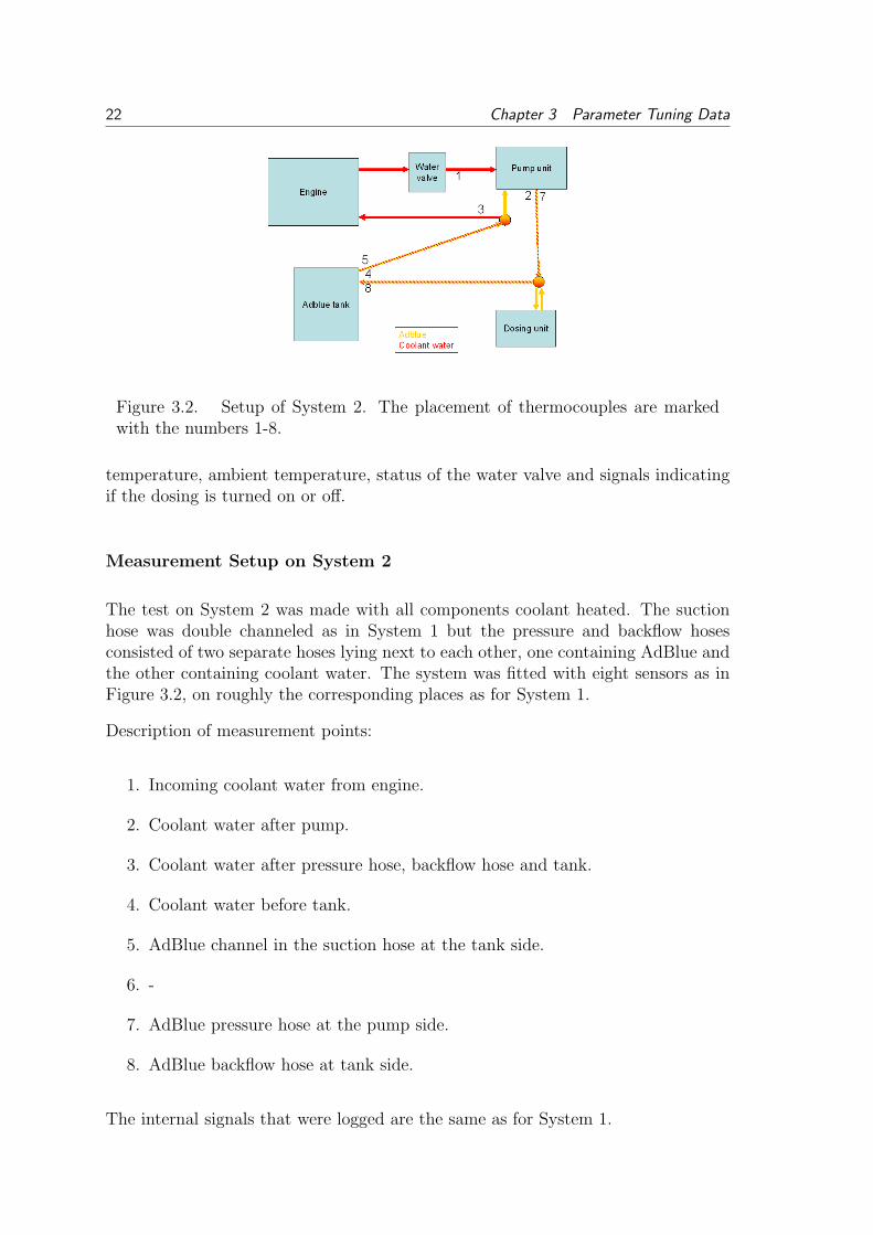
Figure 3.2. Setup of System 2. The placement of thermocouples are markedwith the numbers 1-8.

temperature, ambient temperature, status of the water valve and signals indicatingif the dosing is turned on or off.

Measurement Setup on System 2

The test on System 2 was made with all components coolant heated. The suctionhose was double channeled as in System 1 but the pressure and backflow hosesconsisted of two separate hoses lying next to each other, one containing AdBlue andthe other containing coolant water. The system was fitted with eight sensors as inFigure 3.2, on roughly the corresponding places as for System 1.

Description of measurement points:

1. Incoming coolant water from engine.

2. Coolant water after pump.

3. Coolant water after pressure hose, backflow hose and tank.

4. Coolant water before tank.

5. AdBlue channel in the suction hose at the tank side.

6. -

7. AdBlue pressure hose at the pump side.

8. AdBlue backflow hose at tank side.

The internal signals that were logged are the same as for System 1.


3.1.2 Performed Tests

As mentioned above three tests were done with System 1 and one with System 2.For simplicity and to get a better overview of the tests, the results and observationsfrom each test will be presented directly after the description of the test.

Test 1: System 1 with Assisted Heating

The first test was done to see how the system behaves when heated from a frozenstate under (close to) real conditions. Before the test, to ensure true conditions fora frozen system, the system was left running for a while under normal temperatures.Here leakage on the pressure hose was detected which led to that the two sensorsin the hose unfortunately had to be removed. After that a totally frozen tank wasfitted, with minimal AdBlue and coolant losses. To give the system time to freezethe truck was left overnight in the test cell at a temperature of −20 ◦C.

The main test was done under the following conditions: a constant speed of 30 km/hwith a load of 75 kW throughout the whole test cycle. The ambient temperaturewas held constant at −20 ◦C in about 50 minutes and then changed to −5 ◦C (partlydue to some confusion on how to get the pump started). The water valve was fullyopened during the whole test. When the tank reached the trigger level −8 ◦C thesystem started working.

Results and Observations

As can be seen in Figure 3.3 the four different measurement points differ substan-tially in temperature over time. There can be several reasons for this; one expla-nation is that the two measurements position at the tank end is rather close to thetank armature, which itself conducts the coolant heat better than the hose itself.Another explanation can be that the amount of frozen AdBlue in the vicinity ofthe sensors differs. This can be shown by looking at the temperatures in the regionaround −11 ◦C, in point 5 and 8 there is no ”plateau” which implies that there wereno AdBlue undergoing phase change at that point in the hose. The different lengthof this plateau in the data for point 6 and 7 can also be due to different amountsof frozen AdBlue. When tuning the model, the ”worst-case” should be looked atwhich means the assumption that any point in the hose has the maximal amountof frozen AdBlue. The large temperature drop on all sensors after about 3100 s isbecause the system starts up and colder AdBlue from the tank is pumped into thehoses.

In Figure 3.4a it can be seen that the coolant temperature drop is significant be-tween the first two sensors, a reasonable assumption is that the main part of thistemperature drop takes place during the flow through the tank. The temperaturedrop between point 2 and 3 is minimal which is explained by the pump’s relatively


0 500 1000 1500 2000 2500 3000 3500 4000 4500−30

−20

−10

0

10

20

30

40

50

60

70

Time [s]

Tem

pera

ture

[°C

]

Sensor 5sensor 6Sensor 7Sensor 8

Figure 3.3. AdBlue temperature in measurement point 5-8.

small mass compared to the tank.

0 500 1000 1500 2000 2500 3000 3500 4000 4500−40

−20

0

20

40

60

80

100

Time [s]

Tem

pera

ture

[°C

]

Sensor 1Sensor 2Sensor 3

(a) Coolant temperature

0 500 1000 1500 2000 2500 3000 3500 4000 4500−25

−20

−15

−10

−5

0

5

Time [s]

Tem

pera

ture

[°C

]

AdBlue tank temperature

(b) Tank temperature

Figure 3.4. Coolant and tank temperature measured in System 1.

In Figure 3.4b it is shown that the tank temperature increases a lot slower than inthe hoses. This is caused by the much bigger mass. However there is minimal phasechange tendencies around −11 ◦C, probably because there is no stirring in the tank.

Test 2: System 1 Cool Down

Directly after the first test, the cell temperature was set back to−20 ◦C and the truckwas turned off. This was done to give an estimate of how the AdBlue temperaturein the hoses is affected by the ambient temperature. A drawback with this test


was that only the external temperature sensors were recorded, which means thatsensor 9 has to be relied on to give a proper value of the ambient temperature.

Results and Observations

The main conclusion from this test is that the coolant cools down faster than theAdBlue, which is seen in Figure 3.5. This is probably partly because the AdBluechannel has a smaller diameter which makes it more insulated than the coolantchannel.

0 1000 2000 3000 4000 5000 6000 7000 8000 9000−40

−20

0

20

40

Time [s]

Tem

pera

ture

[°C

]

Sensor 5Sensor 6Sensor 7Sensor 8

0 1000 2000 3000 4000 5000 6000 7000 8000 9000−40

−20

0

20

40

Time [s]

Tem

pera

ture

[°C

]


Figure 3.5. The top figure shows AdBlue temperatures from the external mea-surement points in System 1 and the bottom one shows corresponding coolanttemperatures.

Test 3: System 1 with Ambient Heating

When all sensors (except the tank) had reached (−20 ◦C) the ambient temperaturewas changed again, this time to 10 ◦C while the truck was left turned off. This testwas done to further give an idea of the system response to ambient temperaturechanges.

Results and observations

As expected after the second test, just like the cooling the heating of the coolantwas faster than for the AdBlue. This can be seen in Figure 3.6.


0 2000 4000 6000 8000 10000 12000−30

−20

−10

0

Time [s]

Tem

pera

ture

[°C

]

Sensor 5Sensor 6Sensor 7Sensor 8

0 2000 4000 6000 8000 10000 12000−30

−20

−10

0

Time [s]

Tem

pera

ture

[°C

]


Figure 3.6. The top figure shows AdBlue temperatures from the external mea-surement points in System 1 and the bottom one shows corresponding coolanttemperatures.

Test 4: System 2

The plan was that this test was going to be conducted under the same circumstancesas the first System 1 test. However a few events occurred that changed the outcome.The initial conditions were the same; −20 ◦C, 35 km/h and 75 kW load. 16 min-utes into the test the water valve was opened and the system started to heat up.After about 30 minutes the test was abruptly stopped after an exhaust leakage hadtriggered the automatic emergency stop. At the time the pump had just startedbuilding up pressure. To get rid of the exhaust the cell doors were opened and fanswere started. Due to the increase in temperature it was decided to do the rest ofthe test outside the cell. The truck was started and was let running on idle, withthe pump turned off but with heating turned on, until the temperatures had goneup in the whole system.

Results and observations

Due to the nature of this test the conclusions are not obvious. By looking at Fig-ure 3.7a it can be seen that the AdBlue measurement points have very differenttemperatures. This is because the pressure and backflow hoses basically just con-sisted of two hoses lying next to each other. Therefore the heat transfer in thosehoses is much less efficient than in the two channel hose which can be seen by thedifference in temperature from point 5 to 7 and 8 in the initial heating stage. Bylooking at the coolant in Figure 3.7b the temperature drop is minimal in the pump

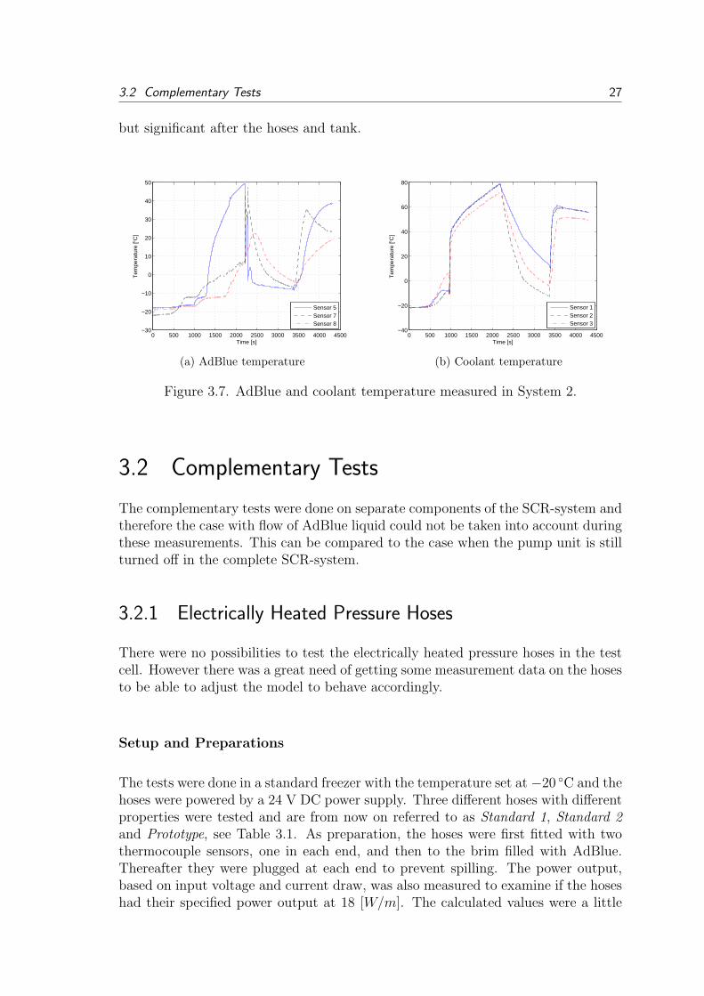
3.2 Complementary Tests 27

but significant after the hoses and tank.

0 500 1000 1500 2000 2500 3000 3500 4000 4500−30

−20

−10

0

10

20

30

40

50

Time [s]

Tem

pera

ture

[°C

]


(a) AdBlue temperature

0 500 1000 1500 2000 2500 3000 3500 4000 4500−40

−20

0

20

40

60

80

Time [s]

Tem

pera

ture

[°C

]


(b) Coolant temperature

Figure 3.7. AdBlue and coolant temperature measured in System 2.

3.2 Complementary Tests

The complementary tests were done on separate components of the SCR-system andtherefore the case with flow of AdBlue liquid could not be taken into account duringthese measurements. This can be compared to the case when the pump unit is stillturned off in the complete SCR-system.

3.2.1 Electrically Heated Pressure Hoses

There were no possibilities to test the electrically heated pressure hoses in the testcell. However there was a great need of getting some measurement data on the hosesto be able to adjust the model to behave accordingly.

Setup and Preparations

The tests were done in a standard freezer with the temperature set at −20 ◦C and thehoses were powered by a 24 V DC power supply. Three different hoses with differentproperties were tested and are from now on referred to as Standard 1, Standard 2and Prototype, see Table 3.1. As preparation, the hoses were first fitted with twothermocouple sensors, one in each end, and then to the brim filled with AdBlue.Thereafter they were plugged at each end to prevent spilling. The power output,based on input voltage and current draw, was also measured to examine if the hoseshad their specified power output at 18 [W/m]. The calculated values were a little


Name Ltot [mm] �out [mm] �in [mm] Pnom [W/m]Standard 1 2240 15 7.3 16.3Standard 2 2000 11.5 5.5 17.6Prototype 680 30 7.3 16.2

Table 3.1. Properties of the electrically heated hoses.

less than this but in all close to the specification. The hoses were then placed in thefreezer and left to freeze during the night.

Test and Results

After the hoses had been completely frozen they were one at a time heated until thetemperature change had slowed down significantly. The measured temperatures foreach hose are shown in Figure 3.8. As can be seen there are differences regardingthe stationary temperature and the time to reach this. The main reasons for thesedifferences can be explained by that there are differences between the hoses regardingthe insulation to the environment and the electrical heat conducted to the AdBlue.

0 1000 2000 3000 4000 5000−20

−10

0

10

20

30

Time [s]

Tem

pera

ture

[°C

]

Sensor 1Sensor 2

(a) Standard 1

0 1000 2000 3000 4000 5000−40

−20

0

20

40

Time [s]

Tem

pera

ture

[°C

]

Sensor 1Sensor 2

(b) Standard 2

0 1000 2000 3000 4000 5000−20

−10

0

10

20

30

40

Time [s]

Tem

pera

ture

[°C

]

Sensor 1Sensor 2

(c) Prototype

Figure 3.8. The heat up process of the hoses. Each hose has values from its twosensors.

3.2.2 Pump 1 & 2

As well as for the electric hoses there were no possibilities to get readings of thepump temperatures in the tests conducted in the test cell. Therefore tests on thetwo different pumps had to be done to get data for the pump model parameters.

3.2 Complementary Tests 29

Setup and Preparations

First both pumps were run in an SCR test rig to fill them with AdBlue under asclose to real conditions as possible. The pumps were then removed and plugged toprevent leakage. Thereafter the pumps were fitted with thermocouples sensors indifferent places inside the pump housing. Pump 1 was fitted with three sensors; oneclose to the AdBlue filter, one near the circuit board and one in the pressure hoseconnector. Pump 2 was more difficult to open and therefore only fitted with twosensors, both in the AdBlue filter.

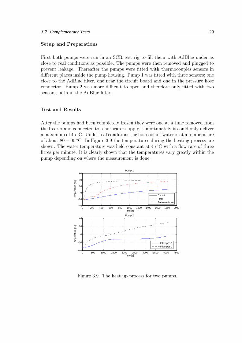
Test and Results

After the pumps had been completely frozen they were one at a time removed fromthe freezer and connected to a hot water supply. Unfortunately it could only delivera maximum of 45 ◦C. Under real conditions the hot coolant water is at a temperatureof about 80− 90 ◦C. In Figure 3.9 the temperatures during the heating process areshown. The water temperature was held constant at 45 ◦C with a flow rate of threelitres per minute. It is clearly shown that the temperatures vary greatly within thepump depending on where the measurement is done.

0 200 400 600 800 1000 1200 1400 1600 1800 2000−40

−20

0

20

40

60

Time [s]

Tem

pera

ture

[°C

]

Pump 1

CircuitFilterPressure hose

0 500 1000 1500 2000 2500 3000 3500 4000 4500−40

−20

0

20

40

Time [s]

Tem

pera

ture

[°C

]

Pump 2

Filter pos 1Filter pos 2

Figure 3.9. The heat up process for two pumps.

4 RESULTS OF THE TEMPERATUREESTIMATION

The tuning parameters for each part of the system, i.e. the heat transfer coefficients,were tuned manually to fit the data from Chapter 3. No specific method for thistuning was used, but the general idea was to find a combination of the two heattransfer coefficients; from the environment to the AdBlue and from the coolant orelectrical heating to the AdBlue. The idea was then to tune the coefficient concerningthe effect from the ambient temperature first and that was done in the cases wheresuch data was available, i.e. for the AdBlue tank and the electrically heated hoses.

The validation of the model is made with temperature data from a new measurementoccasion. These measurements were made at the end of the project in the same testcell and under the same conditions as the measurements in Chapter 3. The resultsare presented for each part of the system and shown as figures containing bothestimated temperature and measured temperature. Analysis of relevant results arealso given for each part.

As will be seen in the results there are two things that have been dealt with inChapter 2 that are excluded from the results; the temperature in each segment andthe effect of the AdBlue flow. Here is an explanation of why that is the case:

• The hose was in Section 2.2.2 divided into segments so that the temperaturecould be estimated in more than one part of the hose. In the actual systemhowever the length of the hoses was too short for any big differences regardingthe coolant water temperature to appear why this could be assumed to beconstant over the length. Another argument for the segments was the temper-ature flow within the liquid Qin and Qout but as this was found to be negligiblecompared to the other heat flows, the effect of the segments disappeared. How-ever, the functionality is still implemented in the model since if longer hoseswould be considered then the temperature loss for the coolant water would bea significant factor.

• The physical flow of AdBlue liquid which for example can be seen in themeasurements in Figure 3.3 as a significant decrease in temperature was alsodiscussed in Section 2.2.2. However since there cannot be any flow of theAdBlue when it is frozen and the main object of the model is to describe thethawing process, the results from simulations with flow enabled has been leftout. As for the segments the functionality is implemented and can be seenas a general behavior when the flow is activated. No effort have been put inparameter tuning though.

30

4.1 Hose Temperature Estimation 31

4.1 Hose Temperature Estimation

In this section the results from the temperature estimation regarding both thecoolant heated hoses and the electrically heated hoses are presented.

4.1.1 Coolant Heated Hoses

The unknown parameters for the coolant heated hoses were adjusted to give a goodfit compared to Sensor 6 in Figure 3.3. A comparison of the estimated and measuredtemperature can be seen in Figure 4.1a. Figure 4.1b shows the AdBlue temperaturein the corresponding sensor for the new measurements on System 2 compared to theestimated. Unfortunately no measurements on any of the double channelled hoseswere made on System 1 on this test occasion. Therefore to get more validationdata for the coolant water heated hoses a test similar to the test of the electricallyheated hoses was done. The hose was filled with AdBlue, given time to freeze andthen connected to a hot water supply with the temperature 45 ◦C. The estimatedtemperature compared to the measured in that test is shown in Figure 4.1c.

0 500 1000 1500 2000 2500 3000−40

−20

0

20

40

60

Time [s]

Tem

pera

ture

[°C

]

Estimated temperatureLogged temperature

(a)

0 500 1000 1500 2000 2500 3000−40

−20

0

20

40

60

Time [s]

Tem

pera

ture

[°C

]


(b)

0 200 400 600 800−20

−10

0

10

20

30

40

50

Time [s]

Tem

pera

ture

[°C

]


(c)

Figure 4.1. Estimated temperature compared to the measured for the coolantwater heated hoses.

4.1.2 Electrically Heated Hoses

As mentioned there were no possibilities to measure the temperature in the elec-trically heated hoses in the test cell, due to leakage. Therefore no validation datafor this part was received. However, to give a picture of how well it is possible toestimate the temperature of this part, the estimated temperature is compared tothe data discussed in Section 3.2.1. The results for the three different types of hosesare shown in Figure 4.2.

32 Chapter 4 Results of the Temperature Estimation

0 1000 2000 3000 4000−20

−10

0

10

20

Time [s]

Tem

pera

ture

[°C

]


(a) Standard 1

0 1000 2000 3000 4000−20

−10

0

10

20

30

40

Time [s]

Tem

pera

ture

[°C

]


(b) Standard 2

0 1000 2000 3000 4000−20

−10

0

10

20

30

40

Time [s]

Tem

pera

ture

[°C

]


(c) Prototype

Figure 4.2. Estimated temperature in comparison to the measured for the threedifferent types of electrically heated hoses.

4.1.3 Analysis of the Hose Temperature Estimation

The temperature estimation in the hoses, both electrically heated and double chan-nelled coolant heated, can be made rather well. However, as can be seen from theresults there are some differences. These may depend on physical phenomenas thateffect the temperature in reality but is not taken into account in the modeling, suchas radiation from the exhaust silencer. Some phenomena are also hard to describewith good accuracy. An example of this is the phase change for the electricallyheated hoses which does not only occur at −11 ◦C but in the interval from −11 ◦Cto 0 ◦C. The reason for this is probably a combination of the sensor position andthe fact that there is no stirring in the hose. If the sensor is close to the hose walland the amount of AdBlue is big enough, the melting will first be local close to thewall and then cooled by the ice from the centre of the hose during its melting. Thetemperature during the phase change measured by the sensor is then not as ”strict”as the model describes it why a local deviation can be seen in this region.

4.2 AdBlue Tank Temperature Estimation

An accurate model of the tank cool down is important for the calculation of initialconditions discussed in Section 2.3. By examining the cool down it is also possibleverify that the impact of the ambient temperature is well modeled. In Figure 4.3,the estimated temperature is compared to measurements. The measurement datais from a winter test where the tank cool down for 10 hours in −3 ◦C was logged.

The measurements of the AdBlue tank temperature during heating was made in theclimate cell for both System 1 and System 2, with ambient temperature −20 ◦C.The tank used in the measurements was the same independent of the system used.The coolant water temperature was similar to the one in Figure 3.4a but the watervalve was not opened until the coolant temperature had reached 45 ◦C. The resultsfor System 1 and 2 are shown in Figure 4.4a and 4.4b.

4.2 AdBlue Tank Temperature Estimation 33

0 0.5 1 1.5 2 2.5 3 3.5 4

x 104

0

5

10

15T

empe

ratu

re [°

C]

Time [s]


Figure 4.3. Estimated temperature compared to measurements for the cooldown of the tank.

0 500 1000 1500 2000 2500 3000 3500−18

−16

−14

−12

−10

−8

Time [s]

Tem

pera

ture

[°C

]


(a) System 1

0 2000 4000 6000 8000−20

−15

−10

−5

0

5

10

Time [s]

Tem

pera

ture

[°C

]


(b) System 2

Figure 4.4. Estimated temperature for the AdBlue tank compared to measure-ments during heating.

34 Chapter 4 Results of the Temperature Estimation

0 500 1000 1500 2000 2500 3000−30

−20

−10

0

10

20

30

40

Time [s]

Tem

pera

ture

[°C

]


(a) System 1

0 500 1000 1500 2000 2500 3000−20

−18

−16

−14

−12

−10

Time [s]

Tem

pera

ture

[°C

]


(b) System 2

Figure 4.5. Estimated pump temperature in comparison to the measured.

4.2.1 Analysis of the AdBlue Tank Temperature Estimation

As can be seen in Figure 4.4 there are some deviations between the estimated tem-perature and the measured. The explanations to this are mainly the same as forthe hoses; radiation from the exhaust silencer is not taken into account and thephase change is more diffuse in reality than in the theory the model is based on. Inthe tank however, the sensor is mounted in a known place and the reason for theconfusion of the phase change is more dependent on how big the region around theheating armature is that shall be taken into account in the model.

4.3 Pump Unit Temperature Estimation

As was seen in Figure 3.9 in Section 3.2.2 the temperature in the pump unit varieda lot depending on where the measurement was done. In the measurement donefor validation data, a hole was drilled into the AdBlue filter in the pump to getmore accurate measurements. Since it had been hard to adjust the parameters fromthe previous data (Figure 3.9), a comparison with that would not be fair. Theparameters were therefore adjusted to fit the new measurements and the results forthe pump unit can be seen more as a measure of how good fit that is possible byadjusting chosen parameters. The results are shown in Figure 4.5a and 4.5b.

5 CONTROL OF ELECTRICAL HEATING

The electrically heated hoses are controlled by a PWM-signal. This means thatthe input voltage is modulated as a series of pulses resulting in a specific averagevoltage over the system. Today a simple on/off control, which triggers on an upperand lower temperature level, is used to control the heating. To examine if this canbe improved, two control methods are suggested and compared to the actual methodregarding thawing time and energy consumption. Since there are no temperaturesensors in the hoses, the output comes from the estimated temperature in the model.The feedback controller calculated in this chapter can be seen as a comparison ofhow much energy that could be saved if a sensor was placed in the hose.

5.1 The Electrically Heated Hose on State SpaceForm

To be able to design controllers, a transfer function of the electrically heated hosesystem from PWM-signal PPWM to AdBlue temperature is needed. For simplicity,the most substantial parts for the heat transfer is chosen to express the systemon state space form. As mentioned, it was found from simulations that Qin andQout could be neglected in comparison to Qenv, Qelec and Qh. With notations as inEquation (2.15)-(2.21) and n = 1, e.g. calculation on one segment, this gives

Th,seg = Qelec −Qh −Qenv =

=1

mhCp,h

(PsegPPWM − hAbAsa,Ab(Th,seg − TAb,seg)+

− henvAsa(Th,seg − Tenv)) (5.1)

TAb,seg = Qh + Qflow =

=1

mAbCp,Ab

(hAbAsa,Ab(Th,seg − TAb,seg)− kflow(TAb,seg−1 − TAb,seg)) (5.2)

A generic state space representation is

x(t) = Ax(t) + Bu(t) + Nv(t)y(t) = Cx(t) + Du(t)

(5.3)

Definex1(t) = Th,seg(t)x2(t) = TAb,seg(t)u(t) = PPWM(t)v1(t) = Tenv(t)v2(t) = TAb,seg−1(t)

(5.4)

35

36 Chapter 5 Control of Electrical Heating

Equation (5.1) and (5.2) can be expressed as

x(t) =

[ −α− β αγ −γ − ζ

]x(t) +

[δ0

]u(t) +

[ε 00 ζ

]v(t)

y(t) =[

0 1]x(t)

(5.5)

whereα =

hAbAsa,Ab

mhCp,h, β = henvAsa

mhCp,h, γ =

hAbAsa,Ab

mAbCp,Ab,

δ = Pseg

mhCp,h, ε = henvAsa

mhCp,h, ζ =

kflow

mAbCp,Ab

The transfer function from input u to output y can then be calculated as (Gladand Ljung 2000)

G(s) = C(sI − A)−1B + D =

=γδ

s2 + s(α + β + γ + ζ) + αζ + β(γ + ζ)(5.6)

As seen in Equation (5.4) there are two different disturbances that has to be takeninto account; ambient temperature, v1(t), which can be seen as a measurable lowfrequent load disturbance, and the physical flow of AdBlue, v2(t).

The AdBlue flow is rather complicated to classify and to compensate for. However,this disturbance has no negative impact on the system since the physical flow requiresthat the AdBlue in the tank is thawed. The temperature of this liquid, whichwill be a dominating factor, is then not a disturbance that the controller has tocompensate for. The controller will therefore only be designed to compensate forthe disturbance from the ambient temperature and the physical AdBlue flow will notbe taken into account, i.e. kflow = 0. With the flow constant to zero, the parameterζ in Equation (5.5) becomes zero and the new transfer function from input to outputis then

G(s) =γδ

s2 + s(α + β + γ) + βγ(5.7)

5.2 Properties of the Different Hoses

As mentioned in Section 3.2.1, three different hoses were tested and these are ex-amined when the controllers are designed. However, since the control design is verysimilar to all hoses, only one hose will be shown for each controller in this report.

From Equation (5.7) the transfer function from PWM-signal to AdBlue temperaturefor each hose is calculated with parameter values for both solid and liquid phase andthe result is shown in Table 5.1. For simplicity, the hoses will from now be referredto their system names given in the same table.

5.2 Properties of the Different Hoses 37

Hose System Transfer func when Transfer func when

name name T < −11 ◦C T > −11 ◦C

Standard 1 G10.01521

s2+0.2826s+0.00035910.00716

s2+0.1668s+0.000169

Standard 2 G20.01143

s2+0.2125s+0.00022930.005379

s2+0.1255s+0.0001079

Prototype G30.01521

s2+0.2819s+0.00019950.00716

s2+0.1661s+9.387∗10−5

Table 5.1. Transfer functions for the electrically heated hoses.

System name Poles Static gain Rise time

G1, T < −11 ◦C −0.2813, −0.0013 42.4 1726G1, T > −11 ◦C −0.1658, −0.0010 42.4 2151G2, T < −11 ◦C −0.2114, −0.0011 49.8 2053G2, T > −11 ◦C −0.1246, −0.0009 49.8 2574G3, T < −11 ◦C −0.2812, −0.0007 76.3 3102G3, T > −11 ◦C −0.1655, −0.0006 76.3 3881

Table 5.2. Properties for System G1, G2 and G3.

To get more knowledge about the systems’ behaviours, the step response is examined(see Figure 5.1). From these it can be seen that all systems seem to be of first ordereven though it is obvious from the transfer functions that they are actually of secondorder. This can be explained by looking at the poles, in Table 5.2. Here it is seenthat all systems have one dominating pole which gives them a first order behaviour(Lennartsson 2006). The dominating pole depends on that the heat transfer fromthe hose material to the AdBlue is fast in comparison to the heat transfer from theelectrical power to the hose material.

0 1000 2000 3000 4000 5000 60000

5

10

15

20

25

30

35

40

45

Step Response

Time (sec)

Am

plitu

de

FrozenLiquid

(a) Step response for G1(s)

0 500 1000 1500 2000 2500 3000 3500 4000 4500 50000

5

10

15

20

25

30

35

40

45

50

Step Response

Time (sec)

Am

plitu

de

FrozenLiquid

(b) Step response for G2(s)

0 1000 2000 3000 4000 5000 6000 7000 8000 9000 100000

10

20

30

40

50

60

70

80

Step Response

Time (sec)

Am

plitu

de

FrozenLiquid

(c) Step response for G3(s)

Figure 5.1. Step response for the three different types of electrically heatedhoses.


5.3 Control Design

With the hoses described by transfer functions as in Table 5.1, controllers can bedesigned based on stability and rise time of the system response from reference signalto output. Three different controllers are designed, one that resembles the currentlyused method and two alternative controllers.

5.3.1 On/off Open-loop Control

The current method used to control the heating of the electric hose is a type ofon/off-control. The idea is that the control signal is either turned fully on or offdepending on if there is a need to heat the hose or not. The main problem withthis method is that the temperature has to be estimated to know when to turn theheating on or off. The advantage is that the control is easy to implement since thecontrol signal only has two values, 0 or 1, which means that no function setting thecontrol signal to an intermediate value is needed. The algorithm is stated as

u(t) =

1 TAb,seg ≤ Tlow

u∗ Tlow < TAb,seg < Thigh

0 TAb,seg ≥ Thigh

(5.8)

where Tlow is the temperature when the heating is to be turned on and Thigh is thetemperature when it is turned off. Between these temperatures the control signal isgiven by u∗ which is given by the rule that if TAb,seg has been greater than Thigh itwill remain 0 until TAb,seg is lower than Tlow. When TAb,seg has been lower than Tlow

the control signal will remain 1 until TAb,seg is greater than Thigh.

The estimation of TAb,seg is in practice based on the ambient and tank temperaturetogether with knowledge about run time and system status. In this report howeverTAb,seg will be based on the model output to get a fair comparison between thecontrol algorithms.

5.3.2 Proportional Open-loop Control

Because there is no way to measure the actual AdBlue temperature in the electrichose, a feedback controller can not be used to control the temperature. Instead anopen-loop controller can be used. Open-loop controllers can be of many differenttypes but the easiest way in this case is to use the ambient temperature togetherwith knowledge about the properties of the hose to develop the control algorithm.

A simple way to control the heating is to base the delivered power on two things; thetime it takes to reach a specific temperature at full electrical power and the powerthat maintains a specific temperature at the given ambient temperature. Withknowledge about this, a simple open-loop controller can be developed.

5.3 Control Design 39

−35 −30 −25 −20 −15 −10 −5 00

1000

2000

3000

4000

Ambient temperature [°C]

Tim

e to

rea

ch 0

°C

[s]

Figure 5.2. The time it takes according to G1 to reach 0 ◦C with differentambient temperatures.

The first thing to start with is the gain of the hose when the ambient temperatureis set to a constant value and the electrical power is turned fully on. In Table 5.2it is seen that for the hose Standard 1 the static gain, |G1(0)|, is 42.4. The modelassumes that the gain is independent of the ambient temperature, i.e. if the heatingis turned fully on the temperature will rise by 42.4 ◦C from the initial temperature.Because the gain is linear, half the power will give half the temperature. This givesthe following relationship for G1 between the PWM-signal, setpoint temperatureand ambient temperature

u(t) =1

|G1(0)|(Tset − Tenv) (5.9)

Using the control signal above, which can be seen as feed-forward of the ambienttemperature, the output will in time reach the set point. However, since the controlsignal is calculated based on the difference between the setpoint and the ambienttemperature a small difference will result in a small control signal. To get a fasterthawing process, the control signal should be set to 1 until the setpoint is reached.Since no feedback is used, the time it takes to reach the setpoint from differentambient temperatures will have to be calculated numerically. This can be doneby using Equation (2.21) but in this case the Simulink model is used to do this.Figure 5.2 shows the time it takes to reach a setpoint of 0 ◦C from different ambienttemperatures. The jump at −11 ◦C is caused by the phase change.

The results above are combined to form the control algorithm which can be describedby

u(t) =

{1 t ≤ tthaw

1|G1(0)|(Tset − Tenv) t > tthaw

(5.10)

where tthaw is the time it takes to reach the setpoint at full power. There are severalways to obtain tthaw, one is to save values for the different temperatures in a tableand get it from there. Another slightly more sophisticated way is to use polynomialsthat fit the curve in Figure 5.2. The following function is used for approximatingthe curve in Figure 5.2

tthaw =

{ −0.10T 3env − 4.20T 2

env − 109.62Tenv + 169.85 Tenv ≤ −11−0.04T 3

env − 0.37T 2env − 26.64Tenv Tenv > −11

(5.11)


5.3.3 Feedback Control

The feedback control is made without an actual sensor for the AdBlue temperature.To base the control on an estimated output would be unwise since even a smallmodel error would make the temperatures drift. A feedback controller is thereforeimplemented in the model for comparison with other controllers. The objective isto examine if the investment in a temperature sensor pays off by the energy savings.To be able to compare the results from the feedback control with other controllers,the same hose is used in these calculations namely Standard 1.

A PI-controller is chosen since it reduces the steady-state error that is given by aP-controller, but it is yet easy to design and implement.

Design of a PI-controller

A general formula for a PI-controller is given by

FPI(s) = Ki1 + Tis

s(5.12)

A strategy for tuning of a feedback controller is to minimize a performance criteriawith demands on stability and the control signal activity (Lennartsson 2006). Forthe hose we have:

• Main criteria for the controller is to compensate for low frequency distur-bances, i.e. ambient temperature, which means minimizing Jv as

Jv =1

Ki

(5.13)

where Ki is the integral gain. The size of Ki is limited by the demands ofstability given by

MS =1

minω |1 + L(jω)| ≤ 1.7 (5.14)

MT = maxω

∣∣∣∣L(jω)

1 + L(jω)

∣∣∣∣ ≤ 1.3 (5.15)

where L(jω) = FPI(jω)G(jω) is the open-loop system. Limits on MS and MT

can be seen as a stability criterion defining the amplitude and phase margin.(Lennartsson 2006)

• The control signal is bounded in between 0 and 1 and there are no demandson the control signal activity within the limits.

5.3 Control Design 41

The design method of the PI-controller is based on choice of the phase margin ϕm

and the cross-over frequency ωc. The phase margin can be seen as a measure of howmuch time delay that can be introduced before the open-loop system gets unstable.The cross-over frequency relates to the response time of the system, where a largecross-over frequency gives a fast system response. Recommended start values are

ϕm = 45◦ (5.16)

ωc = 0.4ωG150 (5.17)

where ωG150 is the frequency when the system’s phase is −150◦. (Lennartsson 2006)

From this Ti and Ki are calculated as

Ti =1

ωc tan(−∠FPI(jωc))(5.18)

Ki =ωc

|G(jωc)|√

1 + (ωcTi)2(5.19)

where∠FPI(jωc) = −180◦ + ϕm − ∠G(jωc) (5.20)

and |G(jωc)| and ∠G(jωc) is the gain and the phase of the system at frequency ωc,respectively.

To get Ki as large as possible, i.e. minimize Jv, ϕm and ωc are iterated in an intervalaround their start values. The values of ϕm and ωc that give the largest Ki and stillfulfill the stability criteria (5.14)-(5.15) are chosen.

From this method Ki and Ti are calculated for a PI-controller on each side of -11 ◦Cas

G1(s), T < −11 ◦C ⇒ Ki = 0.14, Ti = 29.7 (5.21)

G1(s), T > −11 ◦C ⇒ Ki = 0.06, Ti = 49.9 (5.22)

with ϕm = 46.7◦ and ωc = 0.37ω150. In the controller, the parameters are changedwhen the temperature passes −11 ◦C.

Since the ambient temperature is measurable it is common to use a feed-forward gainin combination with the feedback to get a faster compensation of the disturbance.However, the dynamics of the system from PWM-signal to AdBlue temperature isfast in comparison to the change of ambient temperature why feedback control isenough to compensate for the disturbance.

A way to evaluate the controller after the design is to examine the sensitivity functionS(jω) to see how well process disturbances are compensated for. In Figure 5.3 themagnitude for this function and for the open-loop system are shown for differentfrequencies. Here it is seen that for low frequencies the magnitude of S(jω) is smallwhich means that low frequency disturbances are well attenuated. This is the sameas saying that the gain of the system is high for low frequencies which can be seenby looking at L(jω).


10−5

10−4

10−3

10−2

10−1

100

101

−150

−100

−50

0

50

100

150

Mag

nitu

de (

dB)

Bode Diagram

L(jω)

S(jω)

Figure 5.3. Magnitude diagram for L(jω) and S(jω).

Due to the fact that the PWM-signal can not be more than 1 or less than 0 the controlsignal becomes saturated if the controller demands values outside these limits. Acommon problem when this occurs is that the I-part of the controller drifts awayto large values since no effect of the changes is seen on the output error. Whenthe control signal is desaturated it will then take time for it to recover which has anegative effect on the output, see Figure 5.4a.

0 200 400 600 800 1000 12000

0.5

1

1.5

Time [s]

Tem

pera

ture

[°C

]

AdBlue temperature without saturationAdBlue temperature with saturation

(a) Without anti-windup

0 200 400 600 800 1000 12000

0.5

1

1.5

Time [s]

Tem

pera

ture

[°C

]

AdBlue temperature with anti−windup

(b) With anti-windup

Figure 5.4. The closed-loop system’s step response with windup and anti-winduprespectively.

To prevent this phenomenon to happen, anti-windup is implemented which meansthat the increase of the integrator part is interrupted if the control signal goes outsideits limits. The results of this can be seen in Figure 5.4b.

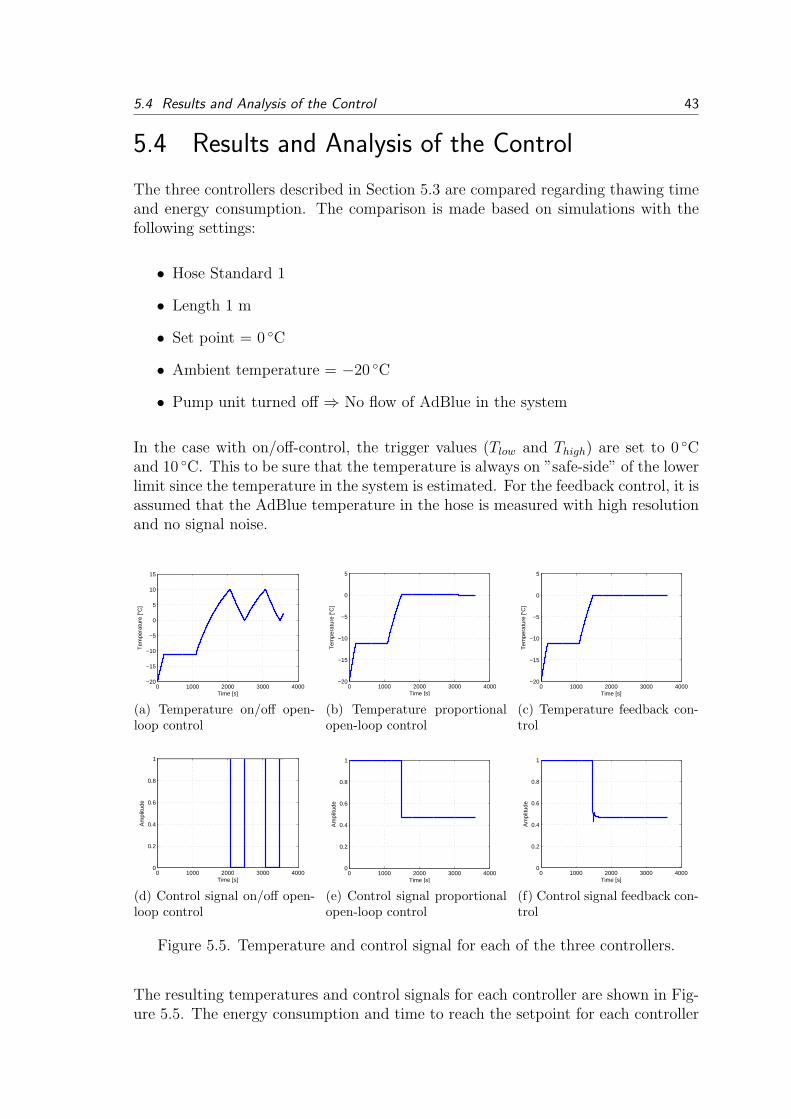
5.4 Results and Analysis of the Control 43

5.4 Results and Analysis of the Control

The three controllers described in Section 5.3 are compared regarding thawing timeand energy consumption. The comparison is made based on simulations with thefollowing settings:

• Hose Standard 1

• Length 1 m

• Set point = 0 ◦C

• Ambient temperature = −20 ◦C

• Pump unit turned off ⇒ No flow of AdBlue in the system

In the case with on/off-control, the trigger values (Tlow and Thigh) are set to 0 ◦Cand 10 ◦C. This to be sure that the temperature is always on ”safe-side” of the lowerlimit since the temperature in the system is estimated. For the feedback control, it isassumed that the AdBlue temperature in the hose is measured with high resolutionand no signal noise.

0 1000 2000 3000 4000−20

−15

−10

−5

0

5

10

15

Time [s]

Tem

pera

ture

[°C

]

(a) Temperature on/off open-loop control

0 1000 2000 3000 4000−20

−15

−10

−5

0

5

Time [s]

Tem

pera

ture

[°C

]

(b) Temperature proportionalopen-loop control

0 1000 2000 3000 4000−20

−15

−10

−5

0

5

Time [s]

Tem

pera

ture

[°C

]

(c) Temperature feedback con-trol

0 1000 2000 3000 40000

0.2

0.4

0.6

0.8

1

Time [s]

Am

plitu

de

(d) Control signal on/off open-loop control

0 1000 2000 3000 40000

0.2

0.4

0.6

0.8

1

Time [s]

Am

plitu

de

(e) Control signal proportionalopen-loop control

0 1000 2000 3000 40000

0.2

0.4

0.6

0.8

1

Time [s]

Am

plitu

de

(f) Control signal feedback con-trol

Figure 5.5. Temperature and control signal for each of the three controllers.

The resulting temperatures and control signals for each controller are shown in Fig-ure 5.5. The energy consumption and time to reach the setpoint for each controller


Control method tset [s] W [kJ ]On/Off 1485 100.1Open-loop 1485 89.32PI 1600 89.21

Table 5.3. Time to reach the setpoint 0 ◦C and energy consumption the firsthour.

0 1000 2000 3000 4000−20

−15

−10

−5

0

5

10

15

Time [s]

Tem

pera

ture

[°C

]

(a) Proportional open-loop control

0 1000 2000 3000 4000−20

−15

−10

−5

0

5

Time [s]

Tem

pera

ture

[°C

]

(b) Feedback control

Figure 5.6. Temperature using the Prototype hose using the same controllerparameters.

are shown in Table 5.3. The energy consumption W is calculated from the controlsignal as

W =

∫ t

0

P (s)ds (5.23)

where P is the power into the hose.

In Table 5.3 the time to reach the setpoint is longer for the PI-controller than forthe other controllers. However, the temperature for the PI-controller is very closeto the setpoint at t = 1485 s which can be seen in Figure 5.5.

To see how well the controllers can handle model errors the hose is changed to theone called Prototype and everything else is left unchanged, including the controllerparameters. The results are shown in Figure 5.6. It is clearly seen that the pro-portional open-loop controller fails to reach the setpoint when the hose is changed.

6 DISCUSSION

In this chapter the results are discussed and suggestions of future work are given.A description of what the Simulink model can be used for is also presented.

6.1 Temperature Estimation

As has been obvious in this report, many parameters are not possible to find intables and are therefore adjusted to measurement data. The majority of the datafor these parameter adjustments were given from only one measurement occasion,i.e. the data from Chapter 3, and most of the measurements were made usingexternal thermocouple sensors. As a result from this it can be hard to tell if it isalways the right thing that has been measured and adjusted to. Therefore, to get areliable model more measurements in different setups are needed. Here follows somecomments of the results from the different components.

The AdBlue temperature in the coolant heated hoses was possible to measure atboth measurement occasions. The amount of available data for these hoses wastherefore considered satisfying. However, even though the measurements were madein similar parts of the same type of hoses, the measurement data had significanttemperature variations. To deal with this the ”worst case” temperature was regardedas the parameter tuning value. By more measurements in similar setups, one couldpossibly get a better idea of which temperature that actually is representative inthe general case.

Concerning the electrically heated hoses the major problem was the fact that itwas not possible during the project to measure the AdBlue temperature on thetruck without leakage. The temperature was therefore not possible to measure inany of the two measurement occasions. The problem here is then not just lack ofvalidation data but also the fact that the measured temperatures in the isolatedtests may differ from what the results had been if the measurements would be doneon the real system.

For the AdBlue tank all measurements have been made with a frozen tank and ithas been heated for a relatively short amount of time. The model can predict thetemperature in this time rather well, however there has been no opportunity totest the model accuracy over longer periods i.e. when the temperature has reachedthe stationary point. Further measurements are needed to test this but it wasunfortunately not possible during the time of this project. Also in all tests the tankhas been totally filled and it would be of interest the see how and if the behaviourchanges with other volumes in the tank.

Regarding the pump unit the main problem was the high complexity of its shape

45

46 Chapter 6 Discussion

and mix of material which made the measurements important in the parametertuning of the model. The measurements however was a problem themselves sinceit is hard to tell where the measurement point should be to give the true AdBluetemperature. Therefore the assumption was made that the measurement with adrilled hole into the Adblue filter gave the most reliable data. This data was givenfirst at the second measurement occasion that was made at the end of the projectand therefore no dedicated validation data was avaliable.

To further improve the results in this project more testing is definitely needed. Withmore measurements from different test runs it could be possible to get a better ideaof the model performance. Highest priority has measurements on the pump unitand the electrical heated hoses since this is needed for validation. Further tuning ofthe model parameters or augmenting some parts can also turn out to be necessarywith more reference data.

6.2 Control Methods

From the results in Table 5.3 it is seen that there are rather small differences be-tween the controllers. This is mainly caused by the saturation of the control signalwhich limits the effect on the output from changes on the control signal. However,more properties than thawing time and energy consumption can be regarded whenevaluating the controllers. The following can be said about the different methods:

• On/off open-loop control is simple and easy to implement. The method doesnot require much calculations, but knowledge about the system is needed toget a good estimation of the temperature in the hose. Since this estimation ishard to make and the limits must be put on the ”safe side” the method easilygets energy consuming.

• Proportional open-loop control is possible to implement without investmentsin an extra temperature sensor and gives an energy efficient way of heating.In a final setup of hardware this may be seen as an alternative setup to thecurrent since it is easy to implement without additional hardware but stillenergy saving in comparison with today’s solution. The controller however isvery sensitive to the hose properties and not robust to changes, see Figure 5.6a.To get a reliable controller good measurement data is also needed and smallchanges may require new measurements and design.

• Feedback control demands a sensor in the hose, and today that investmentis not profitable. If a specific temperature in the hose is necessary or a de-mand would be that one must be able to change arbitrarily between hoses,the investment in a sensor could be considered. An example of the controllerrobustness was seen in Figure 5.6b.

6.3 Simulink Model Applications 47

As mentioned the controllers have been evaluated based on simulations and therewere no time or possibilities to try them on the real system. To verify if the con-clusions from the simulations are valid the controllers must be implemented on thereal SCR-system and tried under different circumstances.

6.3 Simulink Model Applications

Except for temperature estimation in the SCR-system the Simulink model can beused for a variety of tasks both concerning software and hardware design. Onehardware application that the model can be used for is when designing the AdBluetank and its heating configuration. Arbitrary values of tank volume and length,diameter and thickness of the coolant pipes can be chosen and evaluated. This waythere is a possibility to get a primary idea of these parameters before ordering aprototype tank. Each prototype that can be avoided means saving a significantamount of money. The same thing goes for the number of measurements; Eachmeasurement requires several hours of preparations from engineers and mechanicsand the actual measurement takes costly time in the testing cells. Every saved hourmeans money that can be used for other things. Another hardware application istesting of electrically heated hoses. With knowledge of its physical properties it ispossible to get an estimation of the performance before actual testing on the hoseitself.

The main software application is testing of different control concepts, mainly forthe electrically heated hoses. Apart from the methods mentioned in this report it isrelatively easy to implement and evaluate other methods.

6.4 Implementation in the Truck Control Unit

There are a number of applications of the model that could be useful if implementedon a truck. The main application is of course to get an estimate of the temperaturein the unmeasurable parts of the system. This together with the estimation of theinitial states would be very useful when a fast and energy efficient heating is wanted.The model can also as mentioned be of use when designing diagnosis functions todetect sensor failures or system malfunctions.

7 CONCLUSIONS

Models describing the temperatures in the different parts of the two SCR-systemsused at Scania have been developed. The parts that have been modeled are theAdblue tank, the pump unit and the suction, backflow and pressure hoses. Themodels are based on physical relations but some tuning parameters exist to enablemodel adjustments to measurement data. To collect measurement data, tests weredone both on complete SCR-systems in a test cell and by separate tests on individualcomponents.

The two models were built up using Matlab/Simulink. A logical structure andmasking of the Simulink blocks make the models easy to understand and usableeven for those with only little experience in Matlab/Simulink. There are a numberof parameters that can be adjusted and tested using the model such as differentenvironmental temperatures, tank volumes and length of the hoses. From this themodel can be a helpful tool for hardware design and controller design for electricallyheated hoses.

With the unknown parameters adjusted to reference data the temperature estima-tion in the different parts of the SCR-system can be done with good results. Thereis some uncertainty concerning the temperatures in the pump units on both systemsbecause of the large temperature variations in different parts of the pumps. For thepump unit in particular, but also for the other components, the main problem is thelack of measurement data. More data needs to be collected to validate the modelfurther.

Based on knowledge from the model, new algorithms for controlling the electricallyheated hoses have been developed and compared to the current on/off-controller, oneopen-loop and one feedback controller. During the thesis work there have been nopossibilities to test these control concepts on the actual system but from simulationsit can be concluded that the feedback controller would not be profitable to realize.The small energy saving in comparison with open-loop solutions does not justify theadditional cost related to the introduction of a new sensor. An alternative is theproportional open-loop controller which, based on simulations, can give an equallyfast thawing but with less energy consumption than today’s method.

48

Bibliography

aus der Wiesche, Stefan (2007). Numerical heat transfer and thermal engineering ofAdBlue (SCR) tanks for combustion engine emission reduction. Applied Ther-mal Engineering, 27, 1790–1798.

BASF Aktiengesellschaft (2005). AdBlue technical leaflet. Ludwigshafen, Germany.www.resnova-m.com/AdBlue__Dati_Tecnici_GB.pdf.

Engman, Daniel (2006). Optimering av ureainsprutning for SCR katalysator.

Ericson, Claes (2007). NOx modelling of a complete diesel engine/SCR system.

Glad, Torkel and Ljung, Lennart (Eds.) (2000). Control Theory Multivariable andNonlinear Methods. Taylor & Francis. London, Great Britain.

Lennartsson, Bengt (Ed.) (2006). Reglerteknikens grunder. 4th edn. Studentlitter-atur. Lund, Sweden.

Lienhard IV, John and Lienhard V, John (Eds.) (2008). A Heat Transfer Textbook.3rd edn. Phlogiston Press. Cambridge Massachusetts, USA.

Ljung, Lennart and Glad, Torkel (Eds.) (1994). Modeling of Dynamic Systems. Pren-tice Hall Information And System Sciences Series. 1st edn. P T R Prentice Hall.Upper Saddle River, NJ.

Nilsson, Magnus (2006). Low temperature benchmark of SCR catalysts.

Nordling, Carl and Osterman, Jonny (Eds.) (2004). Physics Handbook. 7th edn.Studentlitteratur. Lund, Sweden.

Sandler, Stanley I. (2006). Thermodynamics. Kirk-Othmer Encyclopedia of ChemicalTechnology, 24, 641–695.

49

www.resnova-m.com/AdBlue__Dati_Tecnici_GB.pdf

50 BIBLIOGRAPHY

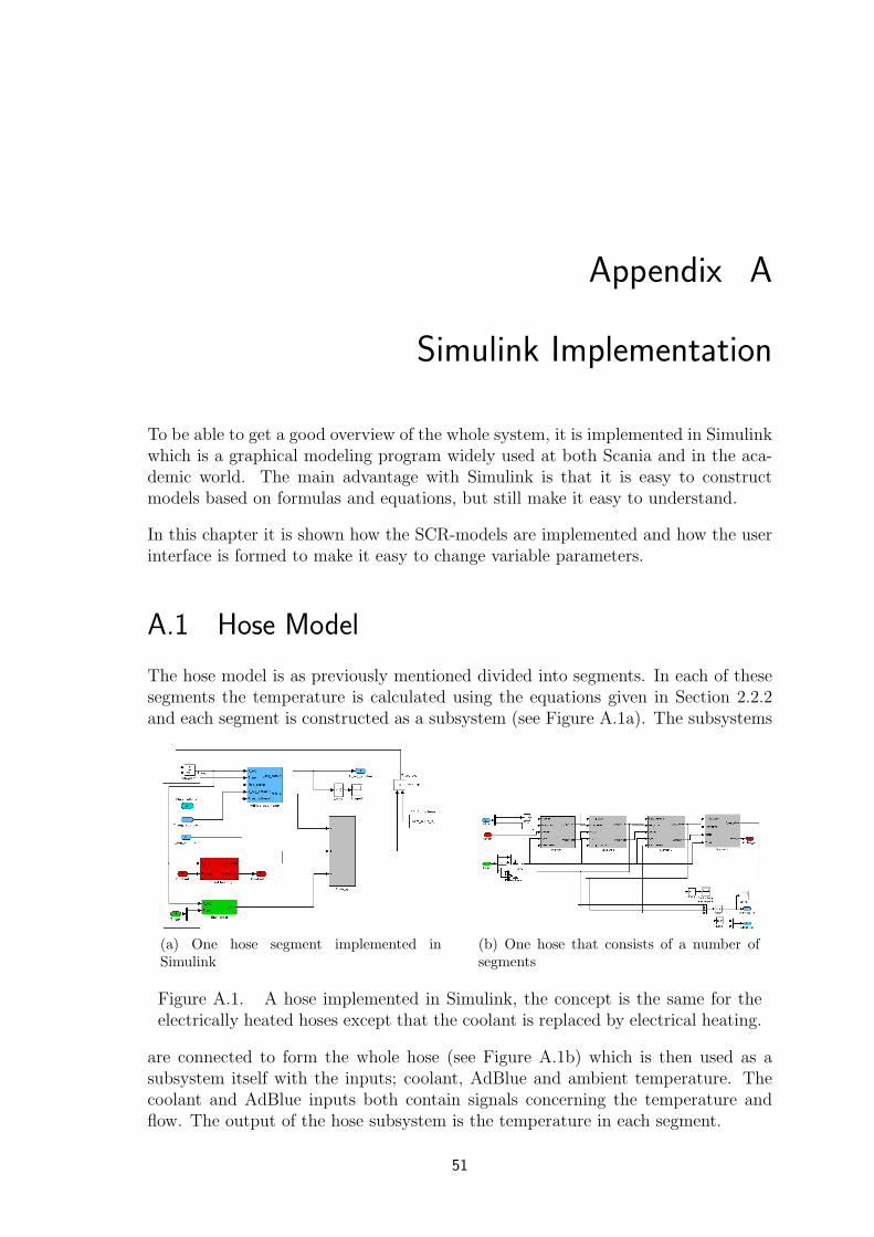
Appendix A

Simulink Implementation

To be able to get a good overview of the whole system, it is implemented in Simulinkwhich is a graphical modeling program widely used at both Scania and in the aca-demic world. The main advantage with Simulink is that it is easy to constructmodels based on formulas and equations, but still make it easy to understand.

In this chapter it is shown how the SCR-models are implemented and how the userinterface is formed to make it easy to change variable parameters.

A.1 Hose Model

The hose model is as previously mentioned divided into segments. In each of thesesegments the temperature is calculated using the equations given in Section 2.2.2and each segment is constructed as a subsystem (see Figure A.1a). The subsystems

(a) One hose segment implemented inSimulink

(b) One hose that consists of a number ofsegments

Figure A.1. A hose implemented in Simulink, the concept is the same for theelectrically heated hoses except that the coolant is replaced by electrical heating.

are connected to form the whole hose (see Figure A.1b) which is then used as asubsystem itself with the inputs; coolant, AdBlue and ambient temperature. Thecoolant and AdBlue inputs both contain signals concerning the temperature andflow. The output of the hose subsystem is the temperature in each segment.

51

52 Appendix A Simulink Implementation

A.2 Tank Model

Based on the equations in Section 2.2.3, the AdBlue tank is implemented as inFigure A.2a. The inputs are the ambient and coolant temperature and output isthe tank temperature.

A.3 Pump Model

Similarly to the tank model the pump unit is implemented using the equationsgiven in Section 2.2.4 (see Figure A.2b). Input is the ambient temperature, and thetemperature and flow of AdBlue and coolant respectively. Output is the temperaturein the pump.

(a) Tank model (b) Pump model

Figure A.2. The AdBlue tank and pump unit models implemented as subsystemsin Simulink.

A.4 Complete SCR-model

The complete model is formed by connecting the subsystems for the three hoses,the tank and the pump. An input data block is also added to define the simulationconditions regarding for example environmental temperature and heating.

A.5 User-Friendly Simulation Environment

To make the model useful even for those with just basic Matlab skills, a simpleinterface is developed. This is done by masking the subsystems and show onlythose parameters the user must be able to change. By double clicking the blocksrepresenting the different components of the SCR-system (seen in Figure A.3) adialog box appear where the properties for each part can be input, see examples in

A.5 User-Friendly Simulation Environment 53

Figure A.3. The complete model of System 1.

Figure A.4.

(a) Properties for thesimulation environment

(b) Inputs for the Ad-Blue tank

Figure A.4. Dialog boxes for initialization of the simulation.

As well as for the initialization it is of importance that the presentation of thesimulation results is simple. Therefore a summary of the temperature in the differentcomponents, as in Figure A.5, is shown when the simulation is stopped. A cross, thatcan be put at a specific temperature and time, makes it easy to compare differentsimulations or see which presumptions that fulfilled a desired criteria.

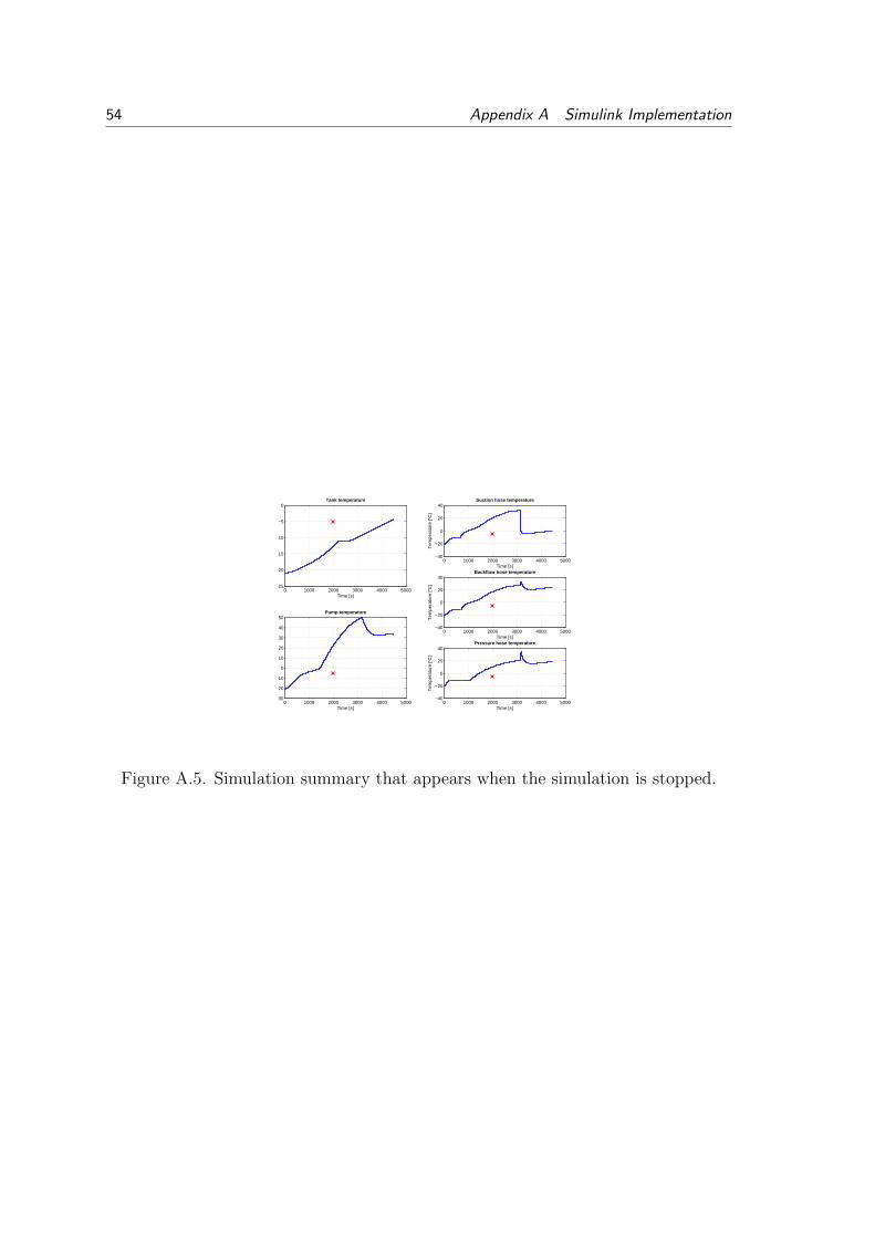
54 Appendix A Simulink Implementation

0 1000 2000 3000 4000 5000−25

−20

−15

−10

−5

0Tank temperature

Time [s]

0 1000 2000 3000 4000 5000−30

−20

−10

0

10

20

30

40

50Pump temperature

Time [s]

0 1000 2000 3000 4000 5000−40

−20

0

20

40Suction hose temperature

Tem

pera

ture

[°C

]

Time [s]

0 1000 2000 3000 4000 5000−40

−20

0

20

40Backflow hose temperature

Tem

pera

ture

[°C

]

Time [s]

0 1000 2000 3000 4000 5000−40

−20

0

20

40Pressure hose temperature

Tem

pera

ture

[°C

]

Time [s]

Figure A.5. Simulation summary that appears when the simulation is stopped.

temperature modeling and control in scr-systems for...

Documents