temperature dependence of viscosity of non-newtonian materials · temperature dependence of...
TRANSCRIPT

Temperature dependence of viscosity of non-Newtonian materials Internship 2012 (May 21st to July 29th) 27.07.2012 TU-Berlin Fanny Rozière Supervisors: B. Emek Abali, M. Sc. & Prof. Dr. rer. nat. Wolfgang H. Müller

2
Table of contents Introduction ........................................................................................................................................................... 3
1. Rheology ........................................................................................................................................................ 3
1.1. The rotational viscometer ...................................................................................................................... 3
Different types of viscometer ......................................................................................................................... 4
1.2. Rheological models ................................................................................................................................ 5
1.3. Different experiments ............................................................................................................................ 6
1.3.1. Flow test ........................................................................................................................................ 6
1.3.2. Creep tests .................................................................................................................................... 6
1.3.3. Oscillatory test ............................................................................................................................... 7
1.4. Quick tutorial for the utilization of the device ......................................................................................... 7
1.4.1. Test procedure .............................................................................................................................. 7
1.4.2. Tricks and notes ............................................................................................................................. 9
2. Inverse analysis .............................................................................................................................................10
3. Results ..........................................................................................................................................................10
3.1. Toothpaste............................................................................................................................................10
3.1.1. Measurements .............................................................................................................................10
3.1.2. Temperature dependence.............................................................................................................11
3.1.3. Oscillatory Test .............................................................................................................................13
3.2. UHU glue ..............................................................................................................................................14
3.2.1. Hardening of UHU glue .................................................................................................................14
3.2.2. Test on hardened glue ..................................................................................................................16
3.3. Strain Gages’ Adhesive ..........................................................................................................................17
3.3.1. Context .........................................................................................................................................17
3.3.2. Flow tests .....................................................................................................................................18
3.3.3. Resistance to temperature ............................................................................................................21
Conclusion .............................................................................................................................................................23
References.............................................................................................................................................................24
Appendix ...............................................................................................................................................................25
Appendix 1: Signal Tooth paste Arctan fits .........................................................................................................25
Appendix 2: Fit graphs for the oscillotary model and the signal toothpaste.........................................................26
Appendix 3: SciPy Code ......................................................................................................................................27
Acknowledgments .................................................................................................................................................32

3
Introduction A knowledge of rheological properties is of importance in processing, handling, process design, product
development and quality control. During these two months of internship, I took an interest in
temperature dependence of rheological behavior of non-Newtonian Material. The work was divided in
two parts. For a first period, by studying a classic rheothinning material, toothpaste, I tried to find a
generic model for the temperature dependence of viscosity. The second part of the work was about
strain gage adhesives in cooperation with the Federal Institute for Materials Research, the aim was here
to learn about the rheological behavior of the material and to connect the results with the industrial
applications.
1. Rheology
Rheology is the material science of amorphous matter with viscous behavior. The response of the
material can be measured with a rheometer, which is necessary to obtain a material model (cf. 1.2).
1.1. The rotational viscometer The measurements have been performed with the rotational viscometer shown in Figure 1.
Figure 1: The rotational Viscometer
The material to test is placed in between two rotating plates. The device shears the material by
controlling the angular velocity or the torque, and so we can study the evolution of the shear stress with
the shear strain rate. The upper plate is turning, the bottom plate is fixed and can be heated from -20°C
to 180°C. The plate is cooled by an external water supply. A compressed air system prevents frictions.

4
This device allows studying the rheological behavior of pasty material and its temperature dependency.
Liquid materials cannot be measured using this method, as it would not stay in-between the two plates.
Different types of viscometer
Two types of rotational viscometer are available in the Laboratory:
Parallel-plates viscometer
Cone-plate viscometer
For a purely sheared material, the angular shear strain γ (cf. Figure 2) is defined as follows:
z
t
)tan( , which implies when γ is small (approximately less than 5°C): z
t
.
Hence the angular shear rate can be written: z
.
Cone-plate viscometer: [1]
In the case of a cone-plate viscometer the upper plate, the upper plate is moved and has the shape of a
cone and the bottom plate is fixed with a flat shape:
Figure 3: Sketch of a cone-plate viscometer
The angular shear rate is thus written: )tan(
x
x
z , and when θ is small: .
So for a cone-plate viscometer, we have the same shear rate for any point M on the cone. That is of
interest, since we want to measure one shear stress versus one shear rate at each instant.
However, for some very stiff materials, the cone may induce some shaping problems. We must also
make sure that θ is small, in order to limit the edge effects.
Parallel-plates viscometer:
In the case of a parallel-plates viscometer, the sample is placed between the two plates and the angular
shear rate can be written:
d
x
z
Figure 2: Pure shear test

5
Figure 4: Sketch of a plate-plate viscometer
Thus on the upper plate, we have an angular shear rate ranging from 0 in the center to d
R at the edge.
For this reason is the cone-plate viscometer better than the parallel-plates viscometer. However we will
have to use the parallel-plates for some stiff materials. Then it is better to choose a small R, so that the
shear rate range is not large.
1.2. Rheological models
For a Newtonian material, the viscosity is defined as follows: ijij d , where )( ij is the stress
tensor and )( ijd is the velocity gradient tensor.
Here we assume that we have a two dimensional problem with only a shear force and strain. Thus the
strain and velocity gradient tensor have the following form:
(
12
12
) and d (
12d
12d
) , where 2
12
d .
Since 12 depends solely on the 12d , we will be able to use one-dimensional models.
Newtonian materials:
A Newtonian material is a purely viscous material with a constant viscosity. The stress depends then
only on the strain rate and the viscosity is defined as follows: .
Non- Newtonian materials:
The studied materials are supposed to be viscoelastic. Under a defined yield stress they behave like
elastic solids. From this yield point, they flow like viscous non-Newtonian fluids, i.e., with a velocity
dependent viscosity.
For those materials, we can define an apparent viscosity using the following models (for instance):
Herschel-Bukley model [2]:
1212 d
nd )( 1212

6
Ziegler Arctan model [3]: ,
where µ, µ’, τ, τ’, n, n’ are constant parameters independent from σ12 and d12.
A non-Newtonian material can be either rheothickening (i.e. it stiffers as the strain rate increases) or
rheothining (i.e. it softens as the strain rate increases). Most non-Newtonian materials are rheothining
and that will be also the case of the materials we will study.
Influence of parameters:
Figure 5: Influence of parameters for the two models
In both cases, n is playing on the curvature, on the slope of the viscous part. For the Herschel-Bukley
model, the material is rheothinning when n is between 0 and 1, and rheothickening when n is
superior to 1. The Arctan model is only valid for rheothinning materials. The stress can be defined as a
kind of yield stress. So by studying and evolution, we can expect to be able to quantify respectively
the viscous and elastic moduli of the material.
1.3. Different experiments
1.3.1. Flow test
A flow test consists in imposing a ramp of stress (resp. strain rate) and measuring the strain rate (resp.
shear stress). It is easy to fit the results (cf. 2.) of this test with the aforementioned models. Flows test
are very easy to proceed and interesting for viscous and time independent materials. In the others case,
we have to mind the fact that we also impose an increasing shear strain on the sample. For the material
suited here, it may not be a problem as far as we have only viscoelacticity and no vicoplasticity. If we
have a viscoplastic material, strain hardening can also happened. If the material is time dependent, we
have the duration of the experiment can change the results.
1.3.2. Creep tests
A creep test consists in imposing and holding a constant stress during a given period of time on the
sample and measuring the strain.
τ'
-1000
-500
0
500
1000
-5 0 5
shea
r st
ress
shear rate
Arctan model
n=∞
n=0,1
n=1
n=0
µ'>µ
-1000
-500
0
500
1000
-5 0 5
She
ar
stre
ss(P
a)
shear rate (s-1)
Herschel-Bulkley model
n=0
n=0,5
n=1
µ=200
)'
arctan('2
' 121212
n
dd
τ

7
Figure 6: Responses to a creep test for a purely elastic or plastic material (a.) and a purely viscous material (b.)
For a purely elastic or plastic solid, we would measure a constant strain, for a purely viscous fluid, a
constant strain rate. This test is mainly useful to study time effect in the behavior of the material.
1.3.3. Oscillatory test
We give in input a shear strain ).sin(0 t on the sample. The shear rate can be written
).cos(0 t .
Let us then define G’ and G’’ as ))cos('')sin('(0 tGtG , we have thus :
''
'G
G .
For a purely elastic material, 0 ='G' and G =G' . For a Newtonian material, 0 =G' and ='G' .
For an oscillatory test, we can impose a sinusoidal strain to the sample with a constant amplitude γ0 and
a ramp of frequency ω and we get in output the two modulus G’ and G’’ vs. the frequency. This method
is thus useful to separate the elastic response of the material (which can be studied with G’) from the
viscous response of the material (which can be studied with G’’).
1.4. Quick tutorial for the utilization of the device
1.4.1. Test procedure
Open the air pressure and the water cooling system before switching on the central unit.
Software : TA Instrument
Checking the plate geometry. To create a new one, click Geometry->New…
Gap
Set 0
Active tab
Figure 7: Setting of geometry

8
The gap (cf. Figure 12) entered as the parameter of the geometry has to match with the
thickness of the sample. It will be used by the software to calculate the shear rate from the
angular velocity.
It is possible to save and open geometries.
Set the zero gap before putting the sample.
Open an existing procedure or create a new one.
Figure 8: Creation of procedure
It is possible to add and change steps even when the experiment has been run.
o Flow procedure: torque, shear stress, angular velocity and strain rate can be imposed.
Maximum torque: 1E5 Nm .
Maximum angular velocity: 100 rads-1 .
o Creep procedure: Shear stress and torque can be fixed.
The case “terminate on equilibrium” is checked by default. In this case, the experiment stops
when strain gets linear vs. time, before the end of the indicated time.
Once the experiment is launched, one can abort the procedure or only the current step which
launches immediately the following step.
Open
procedure
New procedure Add or delete step
9
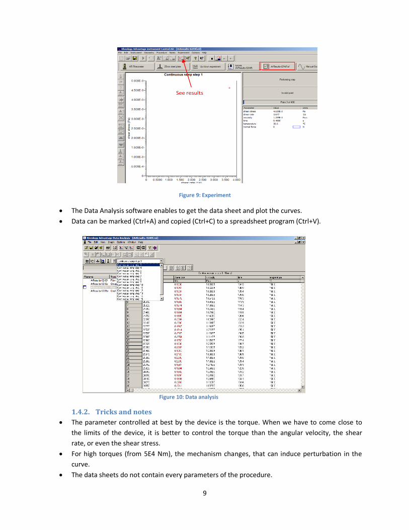
Figure 9: Experiment
The Data Analysis software enables to get the data sheet and plot the curves.
Data can be marked (Ctrl+A) and copied (Ctrl+C) to a spreadsheet program (Ctrl+V).
1.4.2. Tricks and notes
The parameter controlled at best by the device is the torque. When we have to come close to
the limits of the device, it is better to control the torque than the angular velocity, the shear
rate, or even the shear stress.
For high torques (from 5E4 Nm), the mechanism changes, that can induce perturbation in the
curve.
The data sheets do not contain every parameters of the procedure.
Figure 10: Data analysis

10
2. Inverse analysis The data measured have to be fitted with the models presented in chapter 1.2. Using the Inverse
Analysis method, we can fit the shear stress to the shear rate by determining the three parameters , n
and subject to minimizing the mean squared error (cost). This is a non-linear problem, hence a
Newton-Raphson linearization has been utilized. This algorithm is called the Levenberg-Marquardt non-
linear least squares error method. The solving is repeated a large number of times with randomly chosen
starting parameters. Each step gives a new combination of parameters, which is saved if it has a cost less
to the previous ones. This method is a Monte-Carlo method, since it uses a random choice of
parameters. It does not give the best solution, but it approaches it with increasing number of steps
increases. This algorithm is implemented in a Python code (using numpy and Scipy packages) shown in
Appendix 3: SciPy Code.
3. Results
3.1. Toothpaste
Introduction
Toothpaste is a classic rheothinning and easy to handle material. By measuring toothpaste we can expect
to find some generic model for other rheothinning materials.
3.1.1. Measurements
The measurements have been performed on Signal toothpaste with a cone-plate geometry (with a 6 cm
diameter and an 2 ° angle) as shown in the Figure 1 in p.3.
They have been fit by inverse analysis. We could find out the parameters µ, n, τ minimizing at best the
mean squared error with the Stress/Strain rate experimental curve.
Figure 11: Arctan fit for signal toothpaste at 35°C
For the toothpaste, the Arctan model appears to fit better the data than the Herschel-Bukley one. It is
thus the one that we will use in the following measurements.

11
3.1.2. Temperature dependence
Temperature dependence of the material coefficients plays a significant role. The material is softening
as the temperature increases.
Figure 12: Flow tests on signal toothpaste
Those measurement have been modeled by using the parameter fit (cf. ch. 2) for different temperatures,
the acquired results in Table 1 can also be presented as in Figure 13. The graphs of the fits are to be seen
in Appendix 1: Signal Tooth paste Arctan fits.
Table 1: Temperature dependence of parameters for Signal toothpaste
0
50
100
150
200
250
0,00E+00 2,00E-01 4,00E-01 6,00E-01 8,00E-01
Sh
ear
str
ess (
Pa)
Shear rate (s-1)
Signal toothpaste flow tests
20°C25°C30°C35°C40°C45°C50°C
T(°C) T(K) µ(Pa/s) n τ(Pa)
20 293 530 0.029 89
25 298 422 0.036 86
30 303 317 0.059 92
35 308 235 0.065 91
40 313 208 0.030 81
45 318 182 0.019 76
50 323 142 0.024 68
55 328 124 0.0093 56
T↗, µ↘
Change of shape

12
Figure 13: Temperature dependence of parameters for Signal toothpaste
For the apparent viscosity , we can find out an exponential behavior.
For and n , there is no easy to find trend but we can notice a decrease in the value of from 40°C.
This fall coincide with the change in the shape of the curve that happens on Figure 12: Flow tests on
signal toothpaste from 40°C. For this reason, we can assume that there exists a sort of glass transition at
this temperature.
We could not find anything on glass transition of toothpaste in the literature. However, regarding the
composition of the toothpaste, this value coincides with transition temperature of some of the
components.
The supplier gives the following composition:
Calcium Carbonate, Aqua, Sorbitol, Hydrated Silica, Sodium Lauryl Sulfate, Sodium Silicate, Sodium
Monofluorophosphate, Aroma, Cellulose Gum, Potassium Citrate, Benzyl Alcohol, Sodium Saccharin,
Calcium Glycerophosphate, PEG-32, Limonene, CI 73360
y = 9E+07e-0,041x R² = 0,9831
0
200
400
600
800
1000
1200
280 290 300 310 320 330
µ(P
a/s)
T (K)
µ vs Temperature
0
20
40
60
80
100
290 300 310 320 330
τ(P
a)
T (K)
τ vs Temperature
0
0,01
0,02
0,03
0,04
0,05
0,06
0,07
290 300 310 320 330
n
T (K)
n vs Temperature

13
Among this component, the ones that are often used as thickeners are hydrated Silica and cellulose gum.
Mechanical properties of hydrated Silica depend strongly on the water content, which is unfortunately
not given in the composition. The cellulose gum (or Carboxymethyl cellulose) have a higher glass
transition temperature (about 200°C) according to the temperature. The PEG-32 is a polymer
(Polyethylene glycol). It should melt at 42-46°C (cf.[6]). Hence, the structural change occurring at 40°C
could be due to the melt of PEG-32. However, we don’t know the percentage of each ingredient in the
toothpaste, and a mixture doesn’t necessarily react the same way as each component separated.
3.1.3. Oscillatory Test
The apparent viscosity µ and the yield stress τ seem to have two different behaviors. Hence, it would be
interesting to perform some oscillatory measurement, to be able to study independently the elastic
response (characterized by the τ) and the viscous response of the material (characterized by the µ).
We thus performed some oscillatory tests on the toothpaste (cf. 1.3.3) and we tried to fit it with the
fractional Zener model, which were using Aditya Desai:
(cf. [7]).
Starting from this equation can be found the expressions of the two modulus G’ and G’’:
with .
As the device give in output G’, G’’ and ω, we can use the inverse analysis method to fit the result with
the two expression above. Unfortunately, as it is to be seen on the Figure 14 below, we cannot get a
good fit for this data (the other fit graphs are to be found in Appendix 2: Fit graphs for the oscillotary
model and the signal toothpaste
Figure 14: Fit of the results of oscillatory tests on Signal toothpaste at 20°C with the fractional Zener model- to the left: G’ vs. ω, to the right: G’’ vs. ω
The fractional Zener model does not seem to suit the behavior of Signal toothpaste, but it will be
interesting to find a suitable model in further research.
dt
dG
dt
dG
dt
d ijij
ije
ij
ij 0000 )(
20
)2cos(21
))2)((cos()2(cos('
yy
yyGGG e
20
)2cos(21
))2)((sin()2(sin(''
yy
yyGG
0y

14
Conclusion
Signal toothpaste has a very large dependence on temperature. By fitting with the Arctan model, the experimental results at different temperature, we could find out two different trends for µ and for τ: the apparent viscosity µ follows an exponential behavior with temperature, the yield stress τ decrease from 40°C, which could be due to a kind of glass transition. It could be interesting in further research to find a suitable oscillatory model to be able to separate those two trends and to make further tests to investigate this transition at 40°C.
3.2. UHU glue
Introduction
Studying the rheology of adhesives is necessary to be able to foresee their response to stresses in a
current utilization. In this respect, it is interesting to study the rheological behavior of the fixed adhesive.
The measuring procedure will not be exactly the same as for toothpaste. First the fixed glue is much
stiffer than toothpaste, so we will not use a cone-plate geometry anymore but a parallel-plates geometry
(25mm diameter). The hardening reaction is also to mind and can make the measurement more
complicated.
3.2.1. Hardening of UHU glue
Before starting off the experiment, the adhesive has to be hardened fully.
Flow tests:
By performing the same sort of flow tests, as being the case for toothpaste, we can notice that the
hardening process is a thermally activated reaction, which can be seen in the Figure 15 below.
Figure 15: Flow tests on UHU glue
At higher temperature, we can observe a very fast hardening at the scale of one experiment (each
measurement is performed in 3 minutes). For the first measurement at 45°C (light blue curve), we can
0
500
1000
1500
2000
2500
3000
3500
4000
0 5 10
Shea
r st
ress
(P
a)
Shear rate (s-1)
Flow test on unifixed UHU at different temperatures
20°C exp 186
25°C exp 188
30°C exp 190
40°C exp 192
45°C exp 193
45°C exp 194
15
see a rise at the end of the curve (dashed red circle), and with the following measurement at 45°C (pink
curve), we can see that the material is actually stiffer. There is also a rise in the orange curve (full red
circle) which represents the measurement at 40°C.
We have then two phenomena in competition:
the hardening reaction, which tends to stiffen the material faster when the temperature
increases,
the softening of the material when the temperature increases, as it was observed in toothpaste.
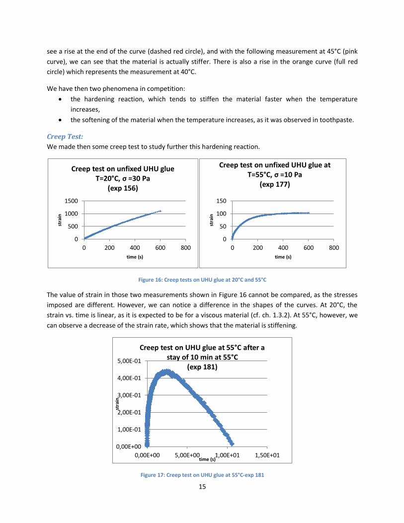
Creep Test:
We made then some creep test to study further this hardening reaction.
Figure 16: Creep tests on UHU glue at 20°C and 55°C
The value of strain in those two measurements shown in Figure 16 cannot be compared, as the stresses
imposed are different. However, we can notice a difference in the shapes of the curves. At 20°C, the
strain vs. time is linear, as it is expected to be for a viscous material (cf. ch. 1.3.2). At 55°C, however, we
can observe a decrease of the strain rate, which shows that the material is stiffening.
Figure 17: Creep test on UHU glue at 55°C-exp 181
0
500
1000
1500
0 200 400 600 800
stra
in
time (s)
Creep test on unfixed UHU glue T=20°C, σ =30 Pa
(exp 156)
0
50
100
150
0 200 400 600 800
stra
in
time (s)
Creep test on unfixed UHU glue at T=55°C, σ =10 Pa
(exp 177)
0,00E+00
1,00E-01
2,00E-01
3,00E-01
4,00E-01
5,00E-01
0,00E+00 5,00E+00 1,00E+01 1,50E+01
stra
in
time (s)
Creep test on UHU glue at 55°C after a stay of 10 min at 55°C
(exp 181)
16
The Figure 17 above represents a creep test performed just after the creep test at 55°C of the Figure 16.
Here we can observe a decrease in the strain, which shows that the material is stiffening very fast. The
material has stiffened and its yield stress became superior to the stress imposed. The glue has thus an
elastic behavior and, as it goes on stiffening, the strain decreases.
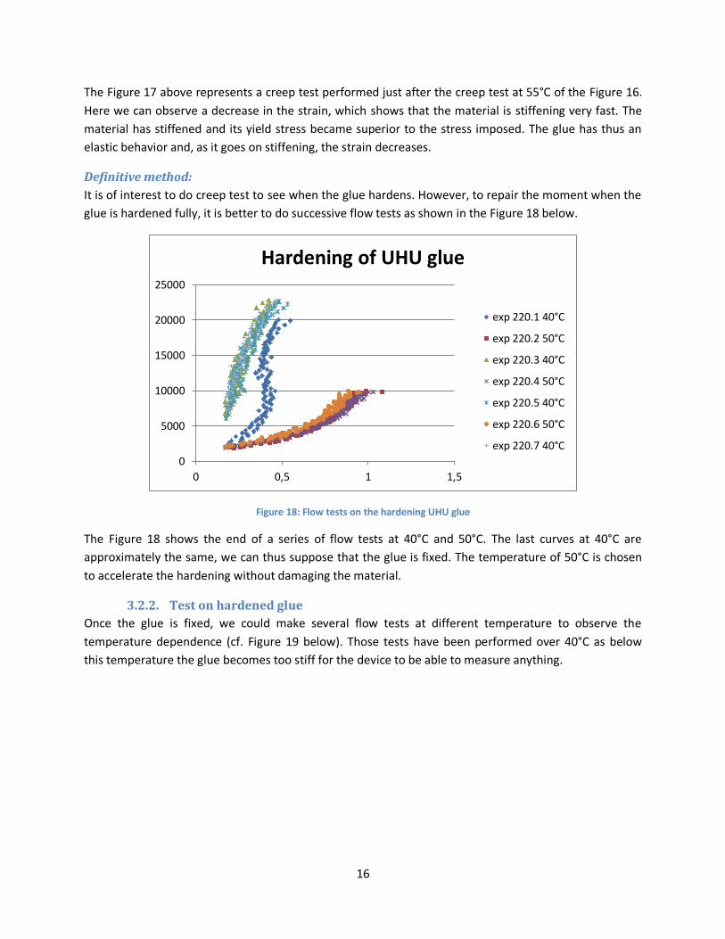
Definitive method:
It is of interest to do creep test to see when the glue hardens. However, to repair the moment when the
glue is hardened fully, it is better to do successive flow tests as shown in the Figure 18 below.
Figure 18: Flow tests on the hardening UHU glue
The Figure 18 shows the end of a series of flow tests at 40°C and 50°C. The last curves at 40°C are
approximately the same, we can thus suppose that the glue is fixed. The temperature of 50°C is chosen
to accelerate the hardening without damaging the material.
3.2.2. Test on hardened glue
Once the glue is fixed, we could make several flow tests at different temperature to observe the
temperature dependence (cf. Figure 19 below). Those tests have been performed over 40°C as below
this temperature the glue becomes too stiff for the device to be able to measure anything.
0
5000
10000
15000
20000
25000
0 0,5 1 1,5
Hardening of UHU glue
exp 220.1 40°C
exp 220.2 50°C
exp 220.3 40°C
exp 220.4 50°C
exp 220.5 40°C
exp 220.6 50°C
exp 220.7 40°C

17
Figure 19: Temperature dependence of UHU glue
As for toothpaste, the temperature plays an important role on the stiffness of the material. However, the
shapes of the curves are not the same, and we could not get any good fit neither with the Arctan model
nor the Herschel-Bulkley model.
Conclusion
To study the rheology of adhesive, the first step is to ensure that they are hardened. Adhesives tend also
to be much more sensitive to temperature, which induces not only a softening but can also play on the
kinetic of chemical reactions. Those elements and methods have to be used for the study of strain gages’
adhesive.
3.3. Strain Gages’ Adhesive A strain gage is a device used to measure strains. The strain gage is stuck on the object to study. The
material is conductive and its electric conduction depends on geometry. It is thus possible to calculate
the strain by measuring the electronic conduction. In this respect, it is important to know the mechanical
properties of the adhesive used, as it can have an influence on the results.
3.3.1. Context
The strain gages’ adhesive studied is the adhesive Kyowa CC33A. The samples have been supplied by the
BAM (Federal Institute for Materials Research and Testing) regarding to a cooperation project. This
adhesive is used for drop test of storage and transport containers. It needs to resist to temperatures
from -60°C to 100°C. The Figure 20 below shows two different types of stain gages.
0
5000
10000
15000
20000
25000
0 2 4 6 8 10 12
She
ar s
tre
ss (
Pa)
Shear rate (s-1)
Evolution with temperature of hardened UHU glue
exp 221.13 40°C
exp 221.1 45°C
exp 221.2 50°C
exp 221.3 55°C
exp 221.4 60°C
exp 221.5 65°C
exp 221.6 70°C
exp 221.8 75°C
exp 221.9 80°C
exp 221.10 85°C
exp 221.11 90°C

18
Figure 20: Strain gages- linear DMS (left) and biaxial DMS (right)
3.3.2. Flow tests
We began the rheological study of the material with flow tests. The
adhesive Kyowa CC33A is a pressure sensitive adhesive. It hardens
pretty fast at room temperature subject to a simple pressure with the
thumb. It also hardens with the pressure of the upper plate going
down on the sample, so we did not have the same sort of problem as
with UHU glue.
However this adhesive is much stiffer than UHU glue, which has caused
two different problems:
The maximum shear stress we can obtain with a 25mm flat
plate, regarding the limit of the device, is around 32kPa. The only
measurements we could get were from 150°C. Below this temperature, the material is too stiff
and imposing a stress of 32 kPa does not enable to measure any strain rate. This temperature is
unfortunately not in the utilization temperature range. However, it could be still interesting to
measure and we can at least say that the adhesive does not show significant strain for a stress
below 32 kPa and a temperature below 150°C.
The adhesive is difficult to unstick at the end of the experiment. We had to use several tricks to
clean it away, as the normal force of the device was not big enough.
Measurement on the prehardened sample:
The first flow test was performed with a prefixed sample from 150°C to 180°C. The data obtained are not
very interesting as far as the sample was much slipping. However we can see on the Figure 22 below that
the sample was kind of “burned” in some places. It was at first totally transparent whereas after the test
we could observe a brown coloration. We can thus assume that there is change occurring in the sample
at this temperature, which we will try to confirm in the following experiment.
Figure 21: The adhesive Kyowa CC33A

19
Figure 22: Prefixed sample after flow tests up to 180°C
Measurements using steel disks:
To protect the bottom plate, we first performed the measurements using one steel disk. The disk is put
on the bottom plate and we use it to set the zero gap. We put then the adhesive to test on the disk. The
measurement shown in Figure 23 has been performed with this steel disk, a 25mm diameter parallel-
plates geometry and a gap of 20µm.
0
5000
10000
15000
20000
25000
30000
0 1 2 3 4
Shea
r st
ress
(Pa)
Shear rate (s-1)
Flow test on Kyowa CC33A at 170°C with one steel disk
Figure 23: Measurement on Kyowa adhesive using a steel disk

20
We make two hypotheses by using this disk:
The steel can be considered as a part of the device, which is reasonable as the plate is also made
of steel, so the mechanical properties must be close.
The disk does not slip on the upper plate, which is much more hazardous. Regarding the results
of the measurements made without the disk (cf. Figure 24), we can assume that on the Figure
23, we measure both the response of the sample and the solid friction between the steel disk
and the bottom plate.
Measurement without disk:
By making the measurement with disks, we could notice that the adhesive was much easier to unstick
after having been kept long enough at high temperature. All the following measurements have thus been
performed using the classic method with a 25 mm diameter parallel-plates geometry and a gap of 20 µm.
To unstick the glue, we had been waited at 180°C until we could raise the plate.
We performed three successive series of flow tests (with the same sample) at temperature ranging from
150°C and 180°C. The Figure 24 below shows the results for the second and the third series.
0
5000
10000
15000
20000
25000
30000
35000
0 5 10 15 20 25 30
she
ar s
tre
ss (
Pa)
Shear rate (s-1)
Flow tests on Kyowa CC33A adhesive exp 240
exp 240.3 150°C
exp 240.5 155°C
exp 240.7 160°C
exp 240.9 165°C
exp 240.11 170°C
exp 240.13 175°C
exp 240.15 180°C

21
Figure 24: Flow tests on Kyowa adhesive - exp 240 & 241
We did not get any data point for the first series of measurements, the material was still too stiff. We can
thus assume that there is a time dependent softening reaction occurring in the material at high
temperature, which induces a structural or a chemical change. Besides this reaction, we can notice the
same sort of reversible softening we could have seen in toothpaste or in UHU glue. As in the case of UHU
glue, we cannot fit those curves with the Herschel-Bulkley or the Arctan model, all the more so as there
is a default in the curves around 12kPa, induced by the device.
3.3.3. Resistance to temperature
We made some creep tests to study its resistance to temperature. We can see on the Figure 25 and
Figure 26 below the results of a creep tests on the adhesive at 180°C. First we imposed a shear stress of
20kPa during 30 minutes (cf. Figure 25). Then for the relaxation step, the stress is put back to 0, and we
have measured the response and the material during 5 minutes (cf. Figure 26).
Figure 25: Creep test on Kyowa adhesive at 180°C exp 241.1
0
5000
10000
15000
20000
25000
30000
35000
0 20 40 60 80 100
She
ar s
tre
ss (
Pa)
Shear rate (s-1)
Flow tests on Kyowa adhesive exp 241
241.3 150°C
241.7 160°C
241.11 170°C
241.15 180°C
0
500
1000
1500
2000
0 500 1000 1500 2000
Stra
in
time (s)
Creep test on strain gauge adhesive at 180°C - σ = 20 kPa
0
2
4
6
8
0 500 1000 1500
Stra
in
time (s)
Zoom

22
We can observe two periods in this first creep test (cf. Figure 25). First, the material reacts like an elastic
solid, i.e., after a short transitory period, the strain tends to be constant, which can be seen in the zoom
(Figure 25-2). From t=25 minutes, the material begins to flow. We can then assume that from this
moment, the yield stress became inferior to 20 kPa, due to this change in the material at high
temperature.
Figure 26: Creep test on Kyowa adhesive at 180°C, Relaxation step - exp 241.2
For the relaxation step, we have a short elastic response at the beginning, and then the strain remains at
1702, which shows the viscous behavior of the adhesive.
We made then a second creep test of 5 minutes with an imposed stress of 20kPa on the same
sample,the results are shown on the Figure 27 below.
Figure 27: Creep test on Kyowa adhesive at 180°C - exp 242
1700170217041706170817101712171417161718
0 50 100 150 200 250 300 350
Stra
in
time(s)
Relaxation step
0
20000
40000
60000
80000
100000
120000
140000
160000
0 200 400 600 800 1000
Stra
in
Time (s)
Creep test II on the Kyowa adhesive at 180°C

23
We can see that the flow of adhesive accelerates, i.e. the strain rate increases. This is the effect of the
softening reaction.
Conclusion:
The device does not enable to study the adhesive at its utilization temperatures. However, we can
characterize its resistance at high temperature by performing a creep test.
Conclusion We had different results by studying Signal toothpaste and adhesives. For Signal toothpaste, we
performed some flow tests at different temperatures and we noticed that the material was softening
with an increasing temperature. After having fit these flow curves with the Arctan model, we have found
two different tendencies for the coefficients µ and τ: an exponential trend for µ between 20°C and 55°C
and a linear decrease from 40°C for τ, which corresponds to a kind of glass transition. We also performed
oscillatory tests and tried to fit it with the fractional Zener model, but this model is unfortunately not
suitable for toothpaste. Further investigations could be useful to study this transition at 40°C and to find
a suitable oscillatory model. It would also be interesting to see if the thermal behavior observed for
toothpaste could be extended to other materials, as a generic model.
The adhesives were much more difficult to study with the rotational viscometer, as we reached the limits
in torque of the device. For the strain gages’ adhesive, we only managed to get measurements above
150°C. We could not find any fit for the Kyowa adhesive. However we could notice two different
phenomena occurring in the material at high temperature: a reversible softening at high temperature, as
it was the case for toothpaste, and a degradation of the material at high temperature, which can be
observed with creep tests. We could notice a fast degradation of the Kyowa adhesive from 25 minutes at
180°C, with a significant decrease in its mechanic properties. In this respect, there are further tests to be
made on the resistance at high temperature of the Kyowa adhesive, maybe by using a more powerful
device.

24
References [1] McKennell R. Cone-plate viscometer, comparison with coaxial cylinder viscometer, Anal. Chem.
28(11), 1710–1714 (1956).
[2] Herschel, W. H., Bulkley, R. Konsistenzmessungen von Gummi-Benzollosungen ¨ . Kolloid-Z. 39, 291-
300 (1926).
[3] Ziegler, H. An introduction to thermomechanics. North Holland, Amsterdam, 1977.
[4] Ziegler, H., Wehrli, C. The derivation of constitutive relations from the free energy and the dissipation
function. Advances in Applied Mechanics 25, 183 – 238 (1987).
[5] B. Emek Abali, Wilhelm Hübner @ LKM - TU Berlin, Computational Reality XIII, Viscometer
(determining material properties), http://www.lkm.tu-berlin.de/ComputationalReality
[6] www.carbowax.com, Technical data sheet, CARBOWAXTM Polyethylene Glycol (PEG) 1450
[7] Chr. Friedrich., Mechanical stress relaxation in polymers: fractional integral model versus fractional
differential model., Journal of Non-Newtonian Fluid Mechanics, 46(23):307 - 314, 1993.

25
Appendix
Appendix 1: Signal Tooth paste Arctan fits
τ
τ
τ τ
τ
τ
τ
τ

26
Appendix 2: Fit graphs for the oscillotary model and the signal toothpaste
G’
G’’

27
Appendix 3: SciPy Code
"""parameter fit"""
__author__ = "B. Emek Abali ([email protected])"
__date__ = "2012-03-23"
__copyright__ = "Copyright (C) 2012, B.E.A."
__license__ = "GNU GPL Version 3 or any later version"
#---------------------------------------------------------------
#---run like: python fit_compute_plot.py
#---from shell after installing FEniCS and SciPy (matplotlib), such that:
#sudo apt-get install python-scipy python-matplotlib
#under Ubuntu
#please refer to:
#---www.fenicsproject.org
#---www.scipy.org
#----------------------------------------------------------------
from dolfin import *
import numpy
#------------reading the data from experiment
#the data Signaldata.py is to be found under Comp.Real. website
shear_stress, shear_rate, viscosity, t, temperature = \
numpy.loadtxt('test.py', unpack=True)
import scipy
import scipy.interpolate
import scipy.optimize
stress = scipy.interpolate.interp1d(shear_rate, shear_stress, bounds_error=False, \

28
fill_value=0.0)
#------------------------------------------parameter identification of the fit equation
def fit2find_param(constitutive_model):
#---model in 1D to be used
def fit(d12,mu,n,tau):
if constitutive_model=='herschelbulkley': sigma = mu*d12**n + tau
if constitutive_model=='arctan': sigma = mu*d12 + \
2.*tau/numpy.pi*numpy.arctan(d12/n)
return sigma
def residual(param, h, G, hypothesis):
return h(G) - hypothesis(G,*param)
def cost(param, h, G, hypothesis):
return numpy.sum(residual(param, h, G, hypothesis)**2,axis=0)
#-----------number of experiments
m=shear_rate.size
#-----------number of them to be taken for fit
m=round(m*0.7)
#-----------initial guess
#as a range, param = [ mu , n , tau ] due to the def fit(d12,mu,n,tau)
prange=[numpy.arange(0,1000,1),numpy.arange(0,1,0.1),numpy.arange(0,10,0.5)]
numpy.seterr(all='ignore')

29
#-------------------------fitting on a random set and testing with another set
montecarlo = 6
number_of_trials = 0
error_min = 10e10
penalty = 10e6
from copy import deepcopy
rate_s=deepcopy(shear_rate)
while number_of_trials < 15000.0:
if montecarlo>5:
p1 = prange[0][numpy.random.random_integers(0,len(prange[0])-1)]
p2 = prange[0][numpy.random.random_integers(0,len(prange[0])-1)]
p3 = prange[0][numpy.random.random_integers(0,len(prange[0])-1)]
param0 = [p1,p2,p3]
montecarlo = 0
numpy.random.shuffle(rate_s)
param_lsq = scipy.optimize.leastsq(residual, param0, \
args=(stress , rate_s[:m], fit))
param=param_lsq[0]
montecarlo +=1
error=cost(param, stress , rate_s[:m], fit)
if param[0]<0: error += penalty #we force tp get k>0
if param[2]<0: error += penalty #we force tp get mu>0
if error<error_min:
chosen_param = param
error_min = error
print 'parameters: ', param, ' error on test set: ', error, \
' @ ', number_of_trials

30
number_of_trials +=1
return chosen_param
#-------------------------------------------parameter identification of the fit equation
#-------------------------------------------------------------------------visualization
import matplotlib as mpl
mpl.use('Agg')
import matplotlib.pyplot as pylab
def visualize(constitutive_model,chosen_param):
def fit(d12,mu,n,tau):
if constitutive_model=='herschelbulkley':
sigma = mu*d12**n + tau
if constitutive_model=='arctan':
sigma = mu*d12 + 2.*tau/numpy.pi*numpy.arctan(d12/n)
return sigma
pylab.cla()
pylab.plot(shear_rate, shear_stress, color='black', marker='+', \
markersize=13, label='data')
pylab.plot(shear_rate, fit(shear_rate,chosen_param[0],chosen_param[1],\
chosen_param[2]), color='red', marker='o', markersize=5, label='fit')
pylab.ylabel('stress $\sigma_{12}$ [Pa]')
pylab.xlabel('velocity gradient $d_{12}$ [1/s]')
pylab.title('Experiment vs. fit')
pylab.legend(loc='best')
pylab.grid(True)
return pylab
#-------------------------------------------------------------------------visualization

31
#------------------------------------------------------------------fit & compute & plot
fit_a = fit2find_param('arctan')
fig_a = visualize('arctan',fit_a)
fig_a.savefig('fit_arctan.png')
"""
fit_hb = fit2find_param('herschelbulkley')
fem_shearrate_hb, fem_stress_hb = compute('herschelbulkley',fit_hb[0],fit_hb[1],fit_hb[2])
fig_hb = visualize('herschelbulkley',fit_hb,fem_shearrate_hb, fem_stress_hb)
fig_hb.savefig('fit_herschelbulkley.ps')
"""
print 80*'-'
print 80*'-'
print 'For arctan model, mu: ',fit_a[0],' n:',fit_a[1],' tau:',fit_a[2]
print 80*'-'
print 80*'-'
"""
print 'For Herschel Bulkley model, mu: ',fit_hb[0],' n:',fit_hb[1],' tau:',fit_hb[2]
print 80*'-'
"""
#---------------------------------------------------------------------------end of file

32
Acknowledgments This research project would not have been possible without the support of many people.
First and foremost, I would like to thank to my mentor Emek Abali, who was abundantly helpful and
offered invaluable guidance and advice, and Professor. Wolfgang H. Müller, the director of the institute,
for his advices and for having me welcomed in the institute.
Thanks to Tabea Wilk from the Federal Institute for Materials Research for providing for me the sample
of strain gage adhesive that I have used in this project.
Thanks also to Maksim Zapara for having shared his office room with Aditya Desai and me and for his
welcome, his help, and his kindness.
Thanks to Aditya Desai for introducing to me his internship work, which has been a great help in my own
project.
Thanks to all the working team of the LKM for its help and welcome.
Finally, thanks to the Rhones-Alpes EXPLORASUP bursary for helping me to enjoy this opportunity.