temperature and precipitation history of the arctic et al 2010 quat... · temperature and...
TRANSCRIPT

lable at ScienceDirect
Quaternary Science Reviews 29 (2010) 1679e1715
Contents lists avai
Quaternary Science Reviews
journal homepage: www.elsevier .com/locate/quascirev
Temperature and precipitation history of the Arctic
G.H. Miller a,*, J. Brigham-Grette b, R.B. Alley c, L. Anderson d, H.A. Bauch e, M.S.V. Douglas f, M.E. Edwards g,S.A. Elias h, B.P. Finney i, J.J. Fitzpatrick d, S.V. Funder j, T.D. Herbert k, L.D. Hinzman l, D.S. Kaufmanm,G.M. MacDonald n, L. Polyak o, A. Robock p, M.C. Serreze q, J.P. Smol r, R. Spielhagen s, J.W.C. White a,A.P. Wolfe f, E.W. Wolff t
a Institute of Arctic and Alpine Research and Department of Geological Sciences, University of Colorado, Boulder, CO 80309-0450, USAbDepartment of Geosciences, University of Massachusetts, Amherst, MA 01003 USAcDepartment of Geosciences and Earth and Environmental Systems Institute, Pennsylvania State University, University Park, PA 16802, USAd Earth Surface Processes, U.S. Geological Survey, MS-980, Box 25046, DFC, Denver, CO 80225, USAeMainz Academy of Sciences, Humanities, and Literature, IFM-GEOMAR, Kiel, GermanyfDepartment of Earth & Atmospheric Sciences, University of Alberta, Edmonton, AB T6G 2E3, Canadag School of Geography, University of Southampton, Highfield, Southampton SO17 1BJ, UKhGeography Department, Royal Holloway, University of London, Egham, Surrey TW20 0EX, UKiDepartment of Biological Sciences, Idaho State University, Pocatello, ID 83209, USAjGeological Museum, University of Copenhagen, Øster Voldgade 5-7, DK-1350, Copenhagen K, DenmarkkDepartment of Geological Sciences, Brown University, Box 1846, Providence, RI 02912, USAlWater and Environmental Research Center University of Alaska Fairbanks, Box 755860, Fairbanks, AK 99775, USAm School of Earth Sciences and Environmental Sustainability, Northern Arizona University, Flagstaff, AZ 86011-4099, USAnDepartment of Geography, University of California, Los Angeles, CA 90095, USAoByrd Polar Research Center, The Ohio State University, 108 Scott Hall, 1090 Carmack Road, Columbus, OH 43210-1002, USApDepartment of Environmental Sciences, Rutgers University, 14 College Farm Road, New Brunswich, NJ 08901, USAqCooperative Institute for Research in Environmental Sciences, NSIDC, University of Colorado, Boulder, CO, USArDepartment of Biology, Queen’s University, Kingston, Ontario K7L 3N6, Canadas Leibniz Institute for Marine Sciences, IFM-GEOMAR, Wischhofstr. 1-3, D-24148 Kiel, GermanytBritish Antarctic Survey, High Cross, Madingley Road, Cambridge CB3 0ET, UK
a r t i c l e i n f o
Article history:Received 2 May 2009Received in revised form20 February 2010Accepted 1 March 2010
* Corresponding author. Tel.: þ1 303 492 6962.E-mail address: [email protected] (G.H. Miller
0277-3791/$ e see front matter � 2010 Elsevier Ltd.doi:10.1016/j.quascirev.2010.03.001
a b s t r a c t
As the planet cooled from peak warmth in the early Cenozoic, extensive Northern Hemisphere ice sheetsdeveloped by 2.6 Ma ago, leading to changes in the circulation of both the atmosphere and oceans. Fromw2.6 to w1.0 Ma ago, ice sheets came and went about every 41 ka, in pace with cycles in the tilt ofEarth’s axis, but for the past 700 ka, glacial cycles have been longer, lasting w100 ka, separated by brief,warm interglaciations, when sea level and ice volumes were close to present. The cause of the shift from41 ka to 100 ka glacial cycles is still debated. During the penultimate interglaciation, w130 to w120 kaago, solar energy in summer in the Arctic was greater than at any time subsequently. As a consequence,Arctic summers werew5 �C warmer than at present, and almost all glaciers melted completely except forthe Greenland Ice Sheet, and even it was reduced in size substantially from its present extent. With theloss of land ice, sea level was about 5 m higher than present, with the extra melt coming from bothGreenland and Antarctica as well as small glaciers. The Last Glacial Maximum (LGM) peaked w21 ka ago,when mean annual temperatures over parts of the Arctic were as much as 20 �C lower than at present.Ice recession was well underway 16 ka ago, and most of the Northern Hemisphere ice sheets had meltedby 6 ka ago. Solar energy reached a summer maximum (9% higher than at present) w11 ka ago and hasbeen decreasing since then, primarily in response to the precession of the equinoxes. The extra energyelevated early Holocene summer temperatures throughout the Arctic 1e3 �C above 20th century aver-ages, enough to completely melt many small glaciers throughout the Arctic, although the Greenland IceSheet was only slightly smaller than at present. Early Holocene summer sea ice limits were substantiallysmaller than their 20th century average, and the flow of Atlantic water into the Arctic Ocean wassubstantially greater. As summer solar energy decreased in the second half of the Holocene, glaciers re-established or advanced, sea ice expanded, and the flow of warm Atlantic water into the Arctic Ocean
).
All rights reserved.

G.H. Miller et al. / Quaternary Science Reviews 29 (2010) 1679e17151680
Fig. 1. Median extent of sea ice in September, 2007, coSeptember 2005. Inset: September sea ice area time serieArctic Ocean summer sea ice in 2007 was greater thanAmerican Geophysical Union.]
diminished. Late Holocene cooling reached its nadir during the Little Ice Age (about 1250e1850 AD),when sun-blocking volcanic eruptions and perhaps other causes added to the orbital cooling, allowingmost Arctic glaciers to reach their maximum Holocene extent. During the warming of the past century,glaciers have receded throughout the Arctic, terrestrial ecosystems have advanced northward, andperennial Arctic Ocean sea ice has diminished.
Here we review the proxies that allow reconstruction of Quaternary climates and the feedbacks thatamplify climate change across the Arctic. We provide an overview of the evolution of climate from thehot-house of the early Cenozoic through its transition to the ice-house of the Quaternary, with specialemphasis on the anomalous warmth of the middle Pliocene, early Quaternary warm times, the MidPleistocene transition, warm interglaciations of marine isotope stages 11, 5e, and 1, the stage 3 inter-stadial, and the peak cold of the last glacial maximum.
� 2010 Elsevier Ltd. All rights reserved.
1. Introduction
Our understanding of the evolution of Arctic climate during theCenozoic has been increasing rapidly, as access to geologicalarchives improves and new tools become available to unravelclimate proxies and to improve both precision and accuracy ofgeochronologies. However, the Cenozoic history of the Arcticremains broadly incomplete. Although there is some evidence toconfirm that the Arctic has cooled from peak warmth in the earlyCenozoic to the ice-age times of the Quaternary, firm networks ofsites capable of defining the spatial patterns of climate are mostlyconfined to a few time-windows of the Quaternary. Reconstructingpast Arctic climates help to reveal key processes of climate change,including the response to elevated greenhouse-gas concentrations,and provide insights into future climate behavior.
Although the Arctic occupies less than 5% of the Earth’s surface,it includes some of the strongest positive feedbacks to climatechange (ACIA, 2005a,b). Over the past 65 Ma the Arctic has expe-rienced a greater change in temperature, vegetation, and oceansurface characteristics than has any other Northern Hemisphere
mpared with averaged intervals dus from 1979 to 2009 based on satellithat predicted by most recent clima
latitudinal band (e.g., Sewall and Sloan, 2001; Bice et al., 2006).Quantitative paleoclimate reconstructions suggest that Arctictemperature changes have been 3e4 times the correspondinghemispheric or globally averaged changes over the past 4 Ma(Miller et al., 2010). These changes impact regions outside theArctic through their proximal influence on the planetary energybalance and circulation of the Northern Hemisphere atmosphereand ocean, and with potential global impacts through changes insea level, the release of greenhouse gases, and impacts on theocean’s meridional overturning circulation.
Recent instrumental records show that during the past fewdecades, surface air temperatures throughout much of the Arctichave risen about twice as fast as temperatures in lower latitudes(Delworth and Knutson, 2000; Knutson et al., 2006). The remark-able reduction in Arctic Ocean summer sea ice in 2007 (Fig. 1)outpaced the most recent predictions from available climatemodels (Stroeve et al., 2008), but it is in concert with widespreadreductions in glacier length, increased borehole temperatures,increased coastal erosion, changes in vegetation and wildlifehabitats, the northward migration of marine life, the evaporation of
ring recent decades. Red curve, 1953e2000; orange curve, 1979e2000; green curve,te imagery (http://nsidc.org/news/press/20091005_minimumpr.html). The reduction inte models. [Copyright 2008 American Geophysical Union, reproduced by permission of
G.H. Miller et al. / Quaternary Science Reviews 29 (2010) 1679e1715 1681
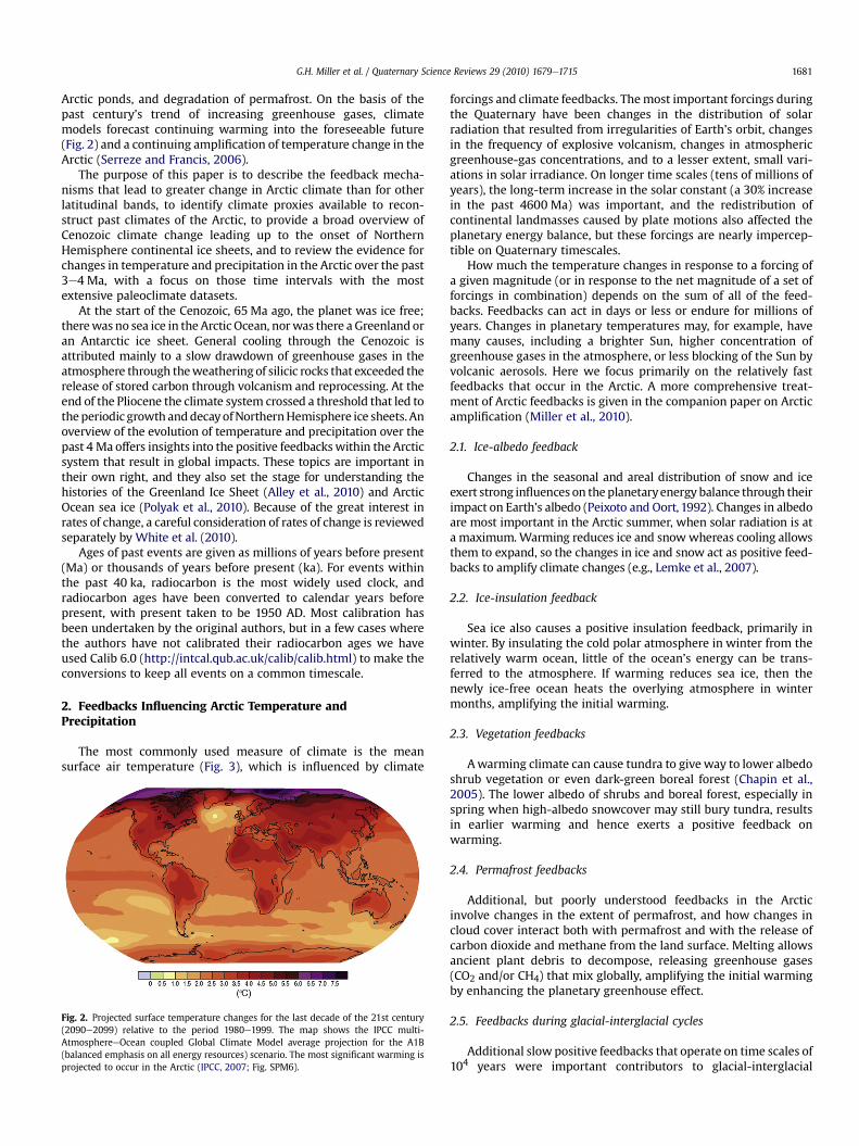
Arctic ponds, and degradation of permafrost. On the basis of thepast century’s trend of increasing greenhouse gases, climatemodels forecast continuing warming into the foreseeable future(Fig. 2) and a continuing amplification of temperature change in theArctic (Serreze and Francis, 2006).
The purpose of this paper is to describe the feedback mecha-nisms that lead to greater change in Arctic climate than for otherlatitudinal bands, to identify climate proxies available to recon-struct past climates of the Arctic, to provide a broad overview ofCenozoic climate change leading up to the onset of NorthernHemisphere continental ice sheets, and to review the evidence forchanges in temperature and precipitation in the Arctic over the past3e4 Ma, with a focus on those time intervals with the mostextensive paleoclimate datasets.
At the start of the Cenozoic, 65 Ma ago, the planet was ice free;therewas no sea ice in the Arctic Ocean, norwas there a Greenland oran Antarctic ice sheet. General cooling through the Cenozoic isattributed mainly to a slow drawdown of greenhouse gases in theatmosphere through theweatheringof silicic rocks that exceeded therelease of stored carbon through volcanism and reprocessing. At theend of the Pliocene the climate system crossed a threshold that led totheperiodic growth anddecayofNorthernHemisphere ice sheets. Anoverview of the evolution of temperature and precipitation over thepast 4 Ma offers insights into the positive feedbackswithin the Arcticsystem that result in global impacts. These topics are important intheir own right, and they also set the stage for understanding thehistories of the Greenland Ice Sheet (Alley et al., 2010) and ArcticOcean sea ice (Polyak et al., 2010). Because of the great interest inrates of change, a careful consideration of rates of change is reviewedseparately by White et al. (2010).
Ages of past events are given as millions of years before present(Ma) or thousands of years before present (ka). For events withinthe past 40 ka, radiocarbon is the most widely used clock, andradiocarbon ages have been converted to calendar years beforepresent, with present taken to be 1950 AD. Most calibration hasbeen undertaken by the original authors, but in a few cases wherethe authors have not calibrated their radiocarbon ages we haveused Calib 6.0 (http://intcal.qub.ac.uk/calib/calib.html) to make theconversions to keep all events on a common timescale.
2. Feedbacks Influencing Arctic Temperature andPrecipitation
The most commonly used measure of climate is the meansurface air temperature (Fig. 3), which is influenced by climate
Fig. 2. Projected surface temperature changes for the last decade of the 21st century(2090e2099) relative to the period 1980e1999. The map shows the IPCC multi-AtmosphereeOcean coupled Global Climate Model average projection for the A1B(balanced emphasis on all energy resources) scenario. The most significant warming isprojected to occur in the Arctic (IPCC, 2007; Fig. SPM6).
forcings and climate feedbacks. Themost important forcings duringthe Quaternary have been changes in the distribution of solarradiation that resulted from irregularities of Earth’s orbit, changesin the frequency of explosive volcanism, changes in atmosphericgreenhouse-gas concentrations, and to a lesser extent, small vari-ations in solar irradiance. On longer time scales (tens of millions ofyears), the long-term increase in the solar constant (a 30% increasein the past 4600 Ma) was important, and the redistribution ofcontinental landmasses caused by plate motions also affected theplanetary energy balance, but these forcings are nearly impercep-tible on Quaternary timescales.
How much the temperature changes in response to a forcing ofa given magnitude (or in response to the net magnitude of a set offorcings in combination) depends on the sum of all of the feed-backs. Feedbacks can act in days or less or endure for millions ofyears. Changes in planetary temperatures may, for example, havemany causes, including a brighter Sun, higher concentration ofgreenhouse gases in the atmosphere, or less blocking of the Sun byvolcanic aerosols. Here we focus primarily on the relatively fastfeedbacks that occur in the Arctic. A more comprehensive treat-ment of Arctic feedbacks is given in the companion paper on Arcticamplification (Miller et al., 2010).
2.1. Ice-albedo feedback
Changes in the seasonal and areal distribution of snow and iceexert strong influences on the planetaryenergy balance through theirimpact on Earth’s albedo (Peixoto and Oort, 1992). Changes in albedoare most important in the Arctic summer, when solar radiation is ata maximum.Warming reduces ice and snowwhereas cooling allowsthem to expand, so the changes in ice and snow act as positive feed-backs to amplify climate changes (e.g., Lemke et al., 2007).
2.2. Ice-insulation feedback
Sea ice also causes a positive insulation feedback, primarily inwinter. By insulating the cold polar atmosphere in winter from therelatively warm ocean, little of the ocean’s energy can be trans-ferred to the atmosphere. If warming reduces sea ice, then thenewly ice-free ocean heats the overlying atmosphere in wintermonths, amplifying the initial warming.
2.3. Vegetation feedbacks
Awarming climate can cause tundra to give way to lower albedoshrub vegetation or even dark-green boreal forest (Chapin et al.,2005). The lower albedo of shrubs and boreal forest, especially inspring when high-albedo snowcover may still bury tundra, resultsin earlier warming and hence exerts a positive feedback onwarming.
2.4. Permafrost feedbacks
Additional, but poorly understood feedbacks in the Arcticinvolve changes in the extent of permafrost, and how changes incloud cover interact both with permafrost and with the release ofcarbon dioxide and methane from the land surface. Melting allowsancient plant debris to decompose, releasing greenhouse gases(CO2 and/or CH4) that mix globally, amplifying the initial warmingby enhancing the planetary greenhouse effect.
2.5. Feedbacks during glacial-interglacial cycles
Additional slow positive feedbacks that operate on time scales of104 years were important contributors to glacial-interglacial
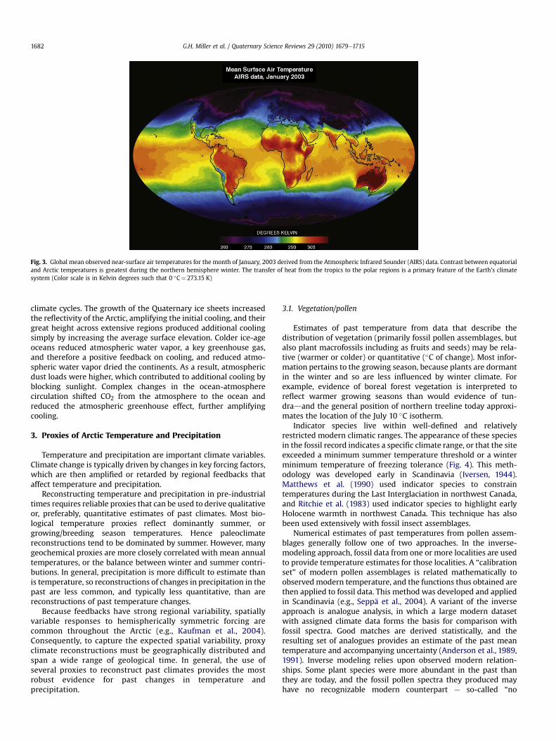
Fig. 3. Global mean observed near-surface air temperatures for the month of January, 2003 derived from the Atmospheric Infrared Sounder (AIRS) data. Contrast between equatorialand Arctic temperatures is greatest during the northern hemisphere winter. The transfer of heat from the tropics to the polar regions is a primary feature of the Earth’s climatesystem (Color scale is in Kelvin degrees such that 0 �C¼ 273.15 K)
G.H. Miller et al. / Quaternary Science Reviews 29 (2010) 1679e17151682
climate cycles. The growth of the Quaternary ice sheets increasedthe reflectivity of the Arctic, amplifying the initial cooling, and theirgreat height across extensive regions produced additional coolingsimply by increasing the average surface elevation. Colder ice-ageoceans reduced atmospheric water vapor, a key greenhouse gas,and therefore a positive feedback on cooling, and reduced atmo-spheric water vapor dried the continents. As a result, atmosphericdust loads were higher, which contributed to additional cooling byblocking sunlight. Complex changes in the ocean-atmospherecirculation shifted CO2 from the atmosphere to the ocean andreduced the atmospheric greenhouse effect, further amplifyingcooling.
3. Proxies of Arctic Temperature and Precipitation
Temperature and precipitation are important climate variables.Climate change is typically driven by changes in key forcing factors,which are then amplified or retarded by regional feedbacks thataffect temperature and precipitation.
Reconstructing temperature and precipitation in pre-industrialtimes requires reliable proxies that can be used to derive qualitativeor, preferably, quantitative estimates of past climates. Most bio-logical temperature proxies reflect dominantly summer, orgrowing/breeding season temperatures. Hence paleoclimatereconstructions tend to be dominated by summer. However, manygeochemical proxies are more closely correlated with mean annualtemperatures, or the balance between winter and summer contri-butions. In general, precipitation is more difficult to estimate thanis temperature, so reconstructions of changes in precipitation in thepast are less common, and typically less quantitative, than arereconstructions of past temperature changes.
Because feedbacks have strong regional variability, spatiallyvariable responses to hemispherically symmetric forcing arecommon throughout the Arctic (e.g., Kaufman et al., 2004).Consequently, to capture the expected spatial variability, proxyclimate reconstructions must be geographically distributed andspan a wide range of geological time. In general, the use ofseveral proxies to reconstruct past climates provides the mostrobust evidence for past changes in temperature andprecipitation.
3.1. Vegetation/pollen
Estimates of past temperature from data that describe thedistribution of vegetation (primarily fossil pollen assemblages, butalso plant macrofossils including as fruits and seeds) may be rela-tive (warmer or colder) or quantitative (�C of change). Most infor-mation pertains to the growing season, because plants are dormantin the winter and so are less influenced by winter climate. Forexample, evidence of boreal forest vegetation is interpreted toreflect warmer growing seasons than would evidence of tun-dradand the general position of northern treeline today approxi-mates the location of the July 10 �C isotherm.
Indicator species live within well-defined and relativelyrestricted modern climatic ranges. The appearance of these speciesin the fossil record indicates a specific climate range, or that the siteexceeded a minimum summer temperature threshold or a winterminimum temperature of freezing tolerance (Fig. 4). This meth-odology was developed early in Scandinavia (Iversen, 1944).Matthews et al. (1990) used indicator species to constraintemperatures during the Last Interglaciation in northwest Canada,and Ritchie et al. (1983) used indicator species to highlight earlyHolocene warmth in northwest Canada. This technique has alsobeen used extensively with fossil insect assemblages.
Numerical estimates of past temperatures from pollen assem-blages generally follow one of two approaches. In the inverse-modeling approach, fossil data from one or more localities are usedto provide temperature estimates for those localities. A “calibrationset” of modern pollen assemblages is related mathematically toobserved modern temperature, and the functions thus obtained arethen applied to fossil data. This method was developed and appliedin Scandinavia (e.g., Seppä et al., 2004). A variant of the inverseapproach is analogue analysis, in which a large modern datasetwith assigned climate data forms the basis for comparison withfossil spectra. Good matches are derived statistically, and theresulting set of analogues provides an estimate of the past meantemperature and accompanying uncertainty (Anderson et al., 1989,1991). Inverse modeling relies upon observed modern relation-ships. Some plant species were more abundant in the past thanthey are today, and the fossil pollen spectra they produced mayhave no recognizable modern counterpart e so-called “no
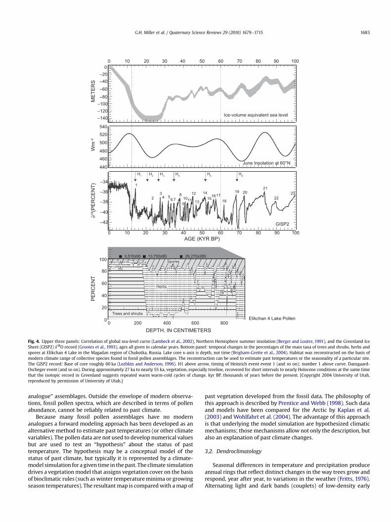
Fig. 4. Upper three panels: Correlation of global sea-level curve (Lambeck et al., 2002), Northern Hemisphere summer insolation (Berger and Loutre, 1991), and the Greenland IceSheet (GISP2) d18O record (Grootes et al., 1993), ages all given in calendar years. Bottom panel: temporal changes in the percentages of the main taxa of trees and shrubs, herbs andspores at Elikchan 4 Lake in the Magadan region of Chukotka, Russia. Lake core x-axis is depth, not time (Brigham-Grette et al., 2004). Habitat was reconstructed on the basis ofmodern climate range of collective species found in fossil pollen assemblages. The reconstruction can be used to estimate past temperatures or the seasonality of a particular site.The GISP2 record: Base of core roughly 60 ka (Lozhkin and Anderson, 1996). H1 above arrow, timing of Heinrich event event 1 (and so on); number 1 above curve, Dansgaard-Oscheger event (and so on). During approximately 27 ka to nearly 55 ka, vegetation, especially treeline, recovered for short intervals to nearly Holocene conditions at the same timethat the isotopic record in Greenland suggests repeated warm warm-cold cycles of change. kyr BP, thousands of years before the present. [Copyright 2004 University of Utah,reproduced by permission of University of Utah.]
G.H. Miller et al. / Quaternary Science Reviews 29 (2010) 1679e1715 1683
analogue” assemblages. Outside the envelope of modern observa-tions, fossil pollen spectra, which are described in terms of pollenabundance, cannot be reliably related to past climate.
Because many fossil pollen assemblages have no modernanalogues a forward modeling approach has been developed as analternative method to estimate past temperatures (or other climatevariables). The pollen data are not used to develop numerical valuesbut are used to test an “hypothesis” about the status of pasttemperature. The hypothesis may be a conceptual model of thestatus of past climate, but typically it is represented by a climate-model simulation for a given time in thepast. The climate simulationdrives a vegetationmodel that assigns vegetation cover on the basisof bioclimatic rules (such aswinter temperatureminima or growingseason temperatures). The resultantmap is comparedwith amap of
past vegetation developed from the fossil data. The philosophy ofthis approach is described by Prentice and Webb (1998). Such dataand models have been compared for the Arctic by Kaplan et al.(2003) and Wohlfahrt et al. (2004). The advantage of this approachis that underlying the model simulation are hypothesized climaticmechanisms; those mechanisms allow not only the description, butalso an explanation of past climate changes.
3.2. Dendroclimatology
Seasonal differences in temperature and precipitation produceannual rings that reflect distinct changes in the way trees grow andrespond, year after year, to variations in the weather (Fritts, 1976).Alternating light and dark bands (couplets) of low-density early
G.H. Miller et al. / Quaternary Science Reviews 29 (2010) 1679e17151684
wood (spring and summer) and higher-density late wood (summerto late summer) have been used to reproduce long time-series ofregional climate change thought to directly influence the produc-tion of meristematic cells in the trees’ vascular cambium, just belowthe bark. Cambial activity in many parts of the northern borealforests can be short; late wood production very likely starts in lateJune and annual-ring width is complete by early August (e.g., Esperand Schweingruber, 2004). Fundamental to the use of tree rings isthe fact that the average width of a tree ring couplet reflects somecombination of environmental factors, largely temperature andprecipitation, but it can also reflect local climatic variables such aswind stress, humidity and soil properties (see Bradley, 1999, forreview). As a general guideline, growing season conditions favor-able for the production of wide annual rings tend to be character-ized bywarmer than average summers with sufficient precipitationto maintain adequate soil moisture. Narrow tree rings occur duringunusually cold or dry growing seasons.
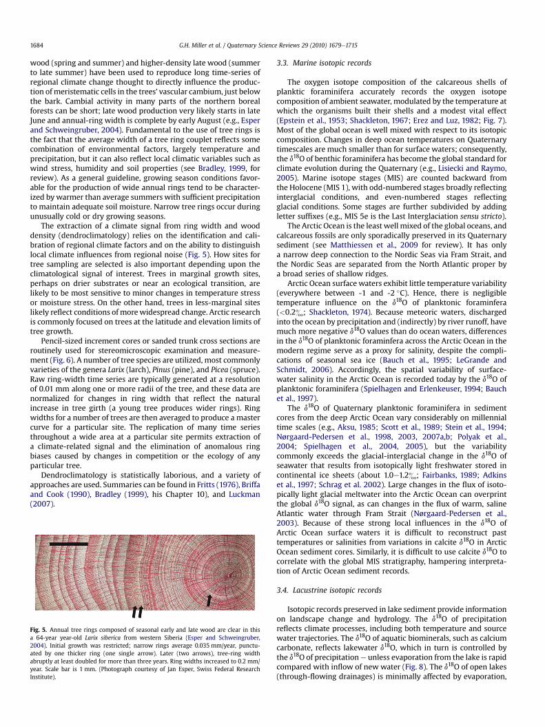
The extraction of a climate signal from ring width and wooddensity (dendroclimatology) relies on the identification and cali-bration of regional climate factors and on the ability to distinguishlocal climate influences from regional noise (Fig. 5). How sites fortree sampling are selected is also important depending upon theclimatological signal of interest. Trees in marginal growth sites,perhaps on drier substrates or near an ecological transition, arelikely to be most sensitive to minor changes in temperature stressor moisture stress. On the other hand, trees in less-marginal siteslikely reflect conditions of morewidespread change. Arctic researchis commonly focused on trees at the latitude and elevation limits oftree growth.
Pencil-sized increment cores or sanded trunk cross sections areroutinely used for stereomicroscopic examination and measure-ment (Fig. 6). A number of tree species are utilized, most commonlyvarieties of the genera Larix (larch), Pinus (pine), and Picea (spruce).Raw ring-width time series are typically generated at a resolutionof 0.01 mm along one or more radii of the tree, and these data arenormalized for changes in ring width that reflect the naturalincrease in tree girth (a young tree produces wider rings). Ringwidths for a number of trees are then averaged to produce a mastercurve for a particular site. The replication of many time seriesthroughout a wide area at a particular site permits extraction ofa climate-related signal and the elimination of anomalous ringbiases caused by changes in competition or the ecology of anyparticular tree.
Dendroclimatology is statistically laborious, and a variety ofapproaches are used. Summaries can be found in Fritts (1976), Briffaand Cook (1990), Bradley (1999), his Chapter 10), and Luckman(2007).
Fig. 5. Annual tree rings composed of seasonal early and late wood are clear in thisa 64-year year-old Larix siberica from western Siberia (Esper and Schweingruber,2004). Initial growth was restricted; narrow rings average 0.035 mm/year, punctu-ated by one thicker ring (one single arrow). Later (two arrows), tree-ring widthabruptly at least doubled for more than three years. Ring widths increased to 0.2 mm/year. Scale bar is 1 mm. (Photograph courtesy of Jan Esper, Swiss Federal ResearchInstitute).
3.3. Marine isotopic records
The oxygen isotope composition of the calcareous shells ofplanktic foraminifera accurately records the oxygen isotopecomposition of ambient seawater, modulated by the temperature atwhich the organisms built their shells and a modest vital effect(Epstein et al., 1953; Shackleton, 1967; Erez and Luz, 1982; Fig. 7).Most of the global ocean is well mixed with respect to its isotopiccomposition. Changes in deep ocean temperatures on Quaternarytimescales are much smaller than for surface waters; consequently,the d18O of benthic foraminifera has become the global standard forclimate evolution during the Quaternary (e.g., Lisiecki and Raymo,2005). Marine isotope stages (MIS) are counted backward fromthe Holocene (MIS 1), with odd-numbered stages broadly reflectinginterglacial conditions, and even-numbered stages reflectingglacial conditions. Some stages are further subdivided by addingletter suffixes (e.g., MIS 5e is the Last Interglaciation sensu stricto).
The Arctic Ocean is the least well mixed of the global oceans, andcalcareous fossils are only sporadically preserved in its Quaternarysediment (see Matthiessen et al., 2009 for review). It has onlya narrow deep connection to the Nordic Seas via Fram Strait, andthe Nordic Seas are separated from the North Atlantic proper bya broad series of shallow ridges.
Arctic Ocean surface waters exhibit little temperature variability(everywhere between -1 and -2 �C). Hence, there is negligibletemperature influence on the d18O of planktonic foraminfera(<0.2&; Shackleton, 1974). Because meteoric waters, dischargedinto the ocean by precipitation and (indirectly) by river runoff, havemuch more negative d18O values than do ocean waters, differencesin the d18O of planktonic foraminfera across the Arctic Ocean in themodern regime serve as a proxy for salinity, despite the compli-cations of seasonal sea ice (Bauch et al., 1995; LeGrande andSchmidt, 2006). Accordingly, the spatial variability of surface-water salinity in the Arctic Ocean is recorded today by the d18O ofplanktonic foraminifera (Spielhagen and Erlenkeuser, 1994; Bauchet al., 1997).
The d18O of Quaternary planktonic foraminifera in sedimentcores from the deep Arctic Ocean vary considerably on millennialtime scales (e.g., Aksu, 1985; Scott et al., 1989; Stein et al., 1994;Nørgaard-Pedersen et al., 1998, 2003, 2007a,b; Polyak et al.,2004; Spielhagen et al., 2004, 2005), but the variabilitycommonly exceeds the glacial-interglacial change in the d18O ofseawater that results from isotopically light freshwater stored incontinental ice sheets (about 1.0e1.2&; Fairbanks, 1989; Adkinset al., 1997; Schrag et al. 2002). Large changes in the flux of isoto-pically light glacial meltwater into the Arctic Ocean can overprintthe global d18O signal, as can changes in the flux of warm, salineAtlantic water through Fram Strait (Nørgaard-Pedersen et al.,2003). Because of these strong local influences in the d18O ofArctic Ocean surface waters it is difficult to reconstruct pasttemperatures or salinities from variations in calcite d18O in ArcticOcean sediment cores. Similarly, it is difficult to use calcite d18O tocorrelate with the global MIS stratigraphy, hampering interpreta-tion of Arctic Ocean sediment records.
3.4. Lacustrine isotopic records
Isotopic records preserved in lake sediment provide informationon landscape change and hydrology. The d18O of precipitationreflects climate processes, including both temperature and sourcewater trajectories. The d18O of aquatic biominerals, such as calciumcarbonate, reflects lakewater d18O, which in turn is controlled bythe d18O of precipitatione unless evaporation from the lake is rapidcompared with inflow of new water (Fig. 8). The d18O of open lakes(through-flowing drainages) is minimally affected by evaporation,

Fig. 6. Typical tree ring samples. (A) Increment cores taken from trees with a small small-bore hollow drill. They can be easily stored and transported in plastic soda straws foranalysis in the laboratory. (B) Alternatively, cross sections or disks can be sanded for study. A cross section of Larix decidua root shows differing wood thickness within single rings,caused by exposure. (Photographs courtesy of Jan Esper and Holger Gärtner, Swiss Federal Research Institute, respectively).
G.H. Miller et al. / Quaternary Science Reviews 29 (2010) 1679e1715 1685
as is d18O in some lakes supplied only by water flow through theground (closed lakes). However, the d18O of closed lakes is at least inpart controlled by lake hydrology. Unless independent evidence oflake hydrology is available, quantitative interpretation of d18O isdifficult. Consequently, d18O is normally combined with additionalclimate proxies to constrain other variables and strengthen inter-pretations. For example, in rare cases, ice core records that arelocated near lakes can provide a d18O record that can aid inter-pretation of the relative contributions of temperature andmoisturesource to the lakewater d18O (Fisher et al., 2004; Anderson and leng,2004; Anderson et al., 2006; Fig. 9). In addition to d18O in carbonateshells, d18O has been measured in diatom silica (Wolfe et al., 1996;Leng andMarshall, 2004; Leng and Barker, 2005; Schiff et al., 2008),and in organic cellulose (Sauer et al., 2001). The isotopic compo-sition of bulk organic matter in lake sediments is complicated bythe possibility of both within-lake and in-washed terrestrial sour-ces. Recent advances in isolating biomarkers unique to aquatic and/or terrestrial sources in sufficient concentration for isotopic anal-yses may circumvent this problem (Huang et al., 2002).
Fig. 7. Microscopic marine plankton known as (foraminiferaifers (see inset) growa shell of calcium carbonate (CaCO3) in or near isotopic equilibrium with ambient seawater. The oxygen isotope ratio measured in these shells can be used to determine thetemperature of the surrounding waters. (The oxygeneisotope ratio is expressed in d18Oparts per million (ppm) ¼ 103[(Rsample/Rstandard)� 1], where Rx¼ (18O)/(16O) is the ratioof isotopic composition of a sample compared to that of an established standard, suchas ocean water. However, factors other than temperature can influence the ratio of 18Oto 16O. Warmer seasonal temperatures, glacial meltwater, and river runoff withdepleted values all will produce a more negative (lighter) d18O ratio. On the other hand,cooler temperatures or higher salinity waters will drive the ratio up, making it heavier,or more positive. The growth of large continental ice sheets selectively removes thelighter isotope (16O), leaving the ocean enriched in the heavier isotope (18O).
3.5. Ice cores
The most common way to deduce temperature from ice cores(Figs. 10 and 11) is through the isotopic content their water, d18Oand dD. Pioneering studies (Dansgaard, 1964) showed that at highnorthern latitudes both d18O and dD are generally considered torepresent themean annual temperature at the core site, and the useof both measures together offers additional information aboutconditions at the source of the water vapor (e.g., Dansgaard et al.,1989). Spatial surveys (Johnsen et al., 1989) and models enabledwith water isotopes (e.g., Hoffmann et al., 1998; Mathieu et al.,2002) show that there exists a strong spatial relationshipbetween temperature and water isotope ratios. The relationship is
d ¼ aT þ b
where T is mean annual surface temperature, and d is annual meand18O or dD value in Arctic precipitation, and the slope, a, has valuestypically around 0.6 for Greenland d18O.
Fig. 8. Lake El’gygytgyn in the Arctic Far East of Russia. Open and closed lake systemsin the Arctic differ hydrologically according to the balance between inflow, outflow,and the ratio of precipitation to evaporation. These parameters are the dominantinfluence on lake stable stable-isotopic chemistry and on the depositional character ofthe sediments and organic matter. Lake El’gygytgyn is annually open and flows to theBering Sea during July and August, but the outlet closes by early September as lakelevel drops and storms move beach gravels that choke the outlet. (Photograph byJ. Brigham-Grette).
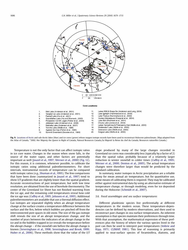
Fig. 9. Locations of Arctic and sub-Arctic lakes (blue) and ice cores (green) whose oxygen isotope records have been used to reconstruct Holocene paleoclimate. (Map adapted fromthe Atlas of Canada, �2002. Her Majesty the Queen in Right of Canada, Natural Resources Canada./Sa Majesté la Reine du chef du Canada, Resources naturelles Canada.)
G.H. Miller et al. / Quaternary Science Reviews 29 (2010) 1679e17151686
Temperature is not the only factor that can affect isotopic ratiosin ice core water. Changes in the season when snow falls, in thesource of the water vapor, and other factors are potentiallyimportant as well (Jouzel et al., 1997; Werner et al., 2000) (Fig. 12).For this reason, it is common, whenever possible, to calibrate theisotopic ratios using additional paleothermometers. For shortintervals, instrumental records of temperature can be comparedwith isotopic ratios (e.g., Shuman et al., 1995). The few comparisonsthat have been done (summarized in Jouzel et al., 1997) tend toshow d/T gradients that are slightly lower than the spatial gradient.Accurate reconstructions of past temperature, but with low timeresolution, are obtained from the use of borehole thermometry. Thecenter of the Greenland Ice Sheet has not finished warming fromthe ice age, and the remaining cold temperatures reveal how coldthe ice age was (Cuffey et al., 1995; Johnsen et al., 1995). Additionalpaleothermometers are available that use a thermal diffusion effect.Gas isotopes are separated slightly when an abrupt temperaturechange at the surface creates a temperature difference between thesurface and the firn, below which bubbles are pinched off from theinterconnected pore spaces in old snow. The size of the gas-isotopeshift reveals the size of an abrupt temperature change, and thenumber of years between the indicators of an abrupt change in theice and in the bubbles trapped in ice reveals the temperature beforethe abrupt change e if the snowfall rate before the abrupt change isknown (Severinghaus et al., 1998; Severinghaus and Brook, 1999;Huber et al., 2006). These methods show that the value of the d/T
slope produced by many of the large changes recorded inGreenland ice cores was considerably less (typically by a factor of 2)than the spatial value, probably because of a relatively largerreduction in winter snowfall in colder times (Cuffey et al., 1995;Werner et al., 2000; Denton et al., 2005). The actual temperaturechanges were therefore larger than would be predicted by thestandard calibration.
In summary, water isotopes in Arctic precipitation are a reliableproxy for mean annual air temperature, but for quantitative use,somemeans of calibrating them is required. They may be calibratedeither against instrumental data by using an alternative estimate oftemperature change, or through modeling, even for ice depositedduring the Holocene (Schmidt et al., 2007).
3.6. Fossil assemblages and sea surface temperatures
Different planktonic species live preferentially at differenttemperatures in the modern ocean. These temperature-depen-dencies can be defined by modern observations, and then used toreconstruct past changes in sea-surface temperatures. An inherentassumption is that speciesmaintain their preferences through time.With that assumption, the mathematical expression of these pref-erences plus the history of where the various species lived in thepast can then be used to interpret past temperatures (Imbrie andKipp, 1971; CLIMAP, 1981). This line of reasoning is primarilyapplied to near-surface species of foraminifera, diatoms, and

Fig. 10. (a) One-meter section of Greenland Ice Core Project-2 core from 1837 m depth showing annual layers. (Photograph courtesy of Eric Cravens, Assistant Curator, U.S. NationalIce Core Laboratory). (b) Field site of Summit Station on top of the Greenland Ice Sheet (Photograph by Michael Morrison, GISP2 SMO, University of New Hampshire; NOAAPaleoslide Set)
G.H. Miller et al. / Quaternary Science Reviews 29 (2010) 1679e1715 1687
dinoflagellates. Such methods are now commonly supported bysea-surface temperature estimates using emerging biomarkertechniques outlined below.
3.7. Biogeochemistry
Within the past decade two new organic proxies have emergedthat can be used to reconstruct past ocean surface temperatures.Both measurements are based on quantifying the proportions ofbiomarkersdmolecules produced by restricted groups of organ-ismsdpreserved in sediments. In the case of the “Uk0
37 index”(Brassell et al.,1986;Prahl et al.,1988), a fewclosely related speciesofcoccolithophorid algae are entirely responsible for producing the37-carbon ketones (alkenones) used in the paleotemperature index,whereas crenarcheota (archea) produce the tetra-ether lipids thatmake up the TEX86 index (Wuchter et al., 2004). Although thespecific function that the alkenones and glycerol dialkyl tetraethersserve for these organisms is unclear, the relationship of thebiomarker Uk0
37 index to temperature has been confirmed experi-mentally in the laboratory (Prahl et al., 1988) and by extensivecalibrations ofmodern surface sediments to overlying surface oceantemperatures (Muller et al., 1998; Wuchter et al., 2004; Conte et al.,
2006). Biomarker compounds appear to be stable over the fullQuaternary (Prahl et al., 1989; Grice et al., 1998; Teece et al., 1998;Herbert, 2003; Schouten et al., 2004). The TEX86 proxy has beenapplied to marine sediments 70e100 million years old.
Biomarker reconstructions have several advantages for recon-structing sea surface conditions in the Arctic. First, in contrast tod18O analyses of marine carbonates (outlined above), the con-founding effects of salinity and ice volume do not compromise theutility of biomarkers as paleotemperature proxies. Both the Uk0
37and TEX86 proxies can be measured reproducibly to high precision(analytical errors correspond to about 0.1 �C for Uk0
37 and 0.5 �C forTEX86), and sediment extractions and gas or liquid chromato-graphic detections can be automated for high sampling rates. Theabundances of biomarkers also provide insights into the composi-tion of past ecosystems, so that links between the physical ocean-ography of the high latitudes and carbon cycling can be assessed.And lastly, organic biomarkers can usually be recovered from Arcticsediments that do not preserve carbonate or siliceous microfossils.It should be noted, however, that the organisms producing thealkenone and tetraethers may have been excluded from the Arcticduring extreme cold periods; thus, continuous records cannot beguaranteed.

Fig. 11. Relation between isotopic composition of precipitation and temperature in theparts of the world where ice sheets exist. Sources of data as follows: InternationalAtomic Energy Agency (IAEA) network (Fricke and O’Neil, 1999; calculated as themeans of summer and winter data of their Table 1 for all sites with complete data).Open squares, poleward of 60� latitude (but with no inland ice-sheet sites); opencircles, 45e60� latitude; filled circles, equatorward of 45� latitude. x, data fromGreenland (Johnsen et al., 1989); þ, data from Antarctica (Dahe et al., 1994). About 71%of Earth’s surface area is equatorward of 45� , where dependence of d18O on temper-ature is weak to nonexistent. Only 16% of Earth’s surface falls in the 45�e60� band, andonly 13% is poleward of 60� . The linear array is clearly dominated by data from the icesheets. (Source: Alley and Cuffey, 2001) [Reproduced by permission MineralogicalSociety of America.]
Fig. 12. Paleotemperature estimates of site and source waters from on Greenland: GRIP andand source (bottom) temperatures derived from GRIP and NorthGRIP d18O and deuterium exline provide an estimate of uncertainties due to the tuning of the isotopic model and the anthe borehole-temperature profile (Dahl-Jensen et al., 1998). [Copyright 2005 American Geo
G.H. Miller et al. / Quaternary Science Reviews 29 (2010) 1679e17151688
The principal caveats in using biomarkers for paleotemperaturereconstructions come from ecological and evolutionary consider-ations. Alkenones are produced by algae that are restricted to thephotic zone, so paleotemperature estimates based on them apply tothis layer, which approximates the sea-surface temperature. In thevast majority of the ocean, the alkenone signal recorded by sedi-ments closely correlates with mean annual sea-surface tempera-ture (Muller et al., 1998; Conte et al., 2006; Fig. 13). However, in thecase of highly seasonal high-latitude oceans, where coccolitho-phorid blooms typically occur during the summer months, thetemperatures inferred from the alkenone Uk0
37 index more closelyapproximates summer, rather than mean-annual sea-surfacetemperatures. A possible complication in past climate states is thatthe season of production may have been highly focused towarda short summer or to a more diffuse late springeearly fallproductive season.
A survey of modern surface sediments in the North Atlantic andNordic Seas (Rosell-Mele et al., 1995) shows that at colder watertemperatures the original unsaturation ratio as defined by Brassellet al. (1986) most reliably estimates surface water temperaturesbecause it includes the Uk0
37:4 alkenone type, which is common inthe Nordic Seas although it is rare or absent in most of the worldocean including the Antarctic. The Brassell et al. (1986) unsatura-tion ratio provides reliable surface water temperature estimates aslow as 6 �C, but errors increase at lower temperatures (Bendle andRosell-Melé, 2004).
Although the marine crenarcheota that produce the tetraethermembrane lipids used in the TEX86 index can range widely throughthewater column, the chemical basis for the TEX86 proxy is fixed by
NorthGrip (Masson-Delmotte et al., 2005). GRIP (left) and NorthGRIP (right) site (top)cess corrected for seawater d18O (until 6000 BP). Shaded lines in gray behind the blackalytical precision. Solid line (in part above zigzag line), GRIP temperature derived fromphysical Union, reproduced by permission of American Geophysical Union.]

Fig. 13. Biomarker alkenone. U37K0
versus measured water temperature for ocean surface mixed layer (0e30 m) samples. (A) Atlantic region. Empirical 3rd-order polynomialregression for samples collected in >4 �C waters is U37
K0 ¼ �1.004�10�4 T3þ 5.744�10�3 T2� 6.207� 10�2 Tþ 0.407 (r2¼ 0.98, n¼ 413) (Outlier data from the southwest Atlanticmargin and northeast Atlantic upwelling regime is excluded.) (B) Pacific, Indian, and Southern Ocean regions: the empirical linear regression of Pacific samples isU37K0 ¼ 0.0391 T� 0.1364 (r2¼ 0.97, n¼ 131). Pacific regression does not include the Indian and Southern Ocean data. (C) Global data: the empirical 3rd order polynomial regression,
excluding anomalous southwest Atlantic margin data, is U37K0 ¼ �5.256�10�5 T3þ 2.884�10�3 T2� 8.4933�10�3 Tþ 9.898 (r2¼ 0.97, n¼ 588). þ¼ sample excluded from
regressions (Conte et al., 2006). [Copyright 2006 American Geophysical Union, reproduced by permission of American Geophysical Union.]
G.H. Miller et al. / Quaternary Science Reviews 29 (2010) 1679e1715 1689

G.H. Miller et al. / Quaternary Science Reviews 29 (2010) 1679e17151690
processes in the photic zone, so that the sedimentary signal origi-nates near the sea surface (Wuchter et al., 2005), just as for the Uk0
37proxy. In situ analyses of particles suspended in the water columnshow that the tetraether lipids are most abundant in winter andspring months in many ocean provinces (Wuchter et al., 2005).
3.8. Biological proxies in lakes
Lakes and ponds are common in most Arctic regions and a widerange of biological climate proxies are preserved in their sediment(Smol and Cumming, 2000; Cohen, 2003; Pienitz et al., 2004;Schindler and Smol, 2006; Smol 2008). Diatom frustules (Douglaset al., 2004) and remains of non-biting flies (chironomid headcapsules; Bennike et al., 2004) are among the biological indicatorsmost commonly used to reconstruct past Arctic climates (Fig. 14).The calibration procedures and statistical treatments are similar tothose described for other proxy indicators (e.g., Birks, 1998). Theresulting mathematical relations are then used to reconstruct theenvironmental variables of interest on the basis of the distributionof indicator assemblages preserved in dated sediment cores (Smol,2008). Where well-calibrated transfer functions are not available,such as for some parts of the Arctic, less-precise climate recon-structions are commonly based on the known ecological and life-history characteristics of the organisms.
3.9. Insect proxies
Insects are common and typically are preserved well in Arcticsediment, primarily in peat. Because many insect types live onlywithin narrow ranges of temperature or other environmental
Fig. 14. Diatom assemblages are determined by a variety of environmental conditions in Aronmental controls such as light, nutrient availability, water chemistry, or temperature. Showwestern Spitsbergen, Svalbard. (A) An abrupt transition from laminated silts to organic sedrainage catchment since end of the Little Ice Age. Recent assemblages (B) are characterizeddiatom assemblages were less diverse and primarily bottom dwelling during the early 20th calgae) (D). Across the Arctic, small diatoms of the Family Fragilariaceae (E) are common inindicate stable limnological conditions for several millennia.
conditions, the remains of particular insects in dated sedimentaccumulations provides useful information on past climates. Cali-brating the observed insect data to climate involves extensivemodern and recent collections, together with careful statisticalanalyses. For example, fossil beetles are typically related totemperature using what is known as the Mutual Climatic Rangemethod (Elias et al., 1999; Bray et al., 2006). This method quanti-tatively assesses the relation between the modern geographicalranges of selected beetle species and modern meteorological data.A “climate envelope” is determined, within which a species canthrive. When used with paleodata, the method allows for thereconstruction of several parameters such as mean temperatures ofthe warmest and coldest months of the year.
3.10. Vegetation-derived precipitation estimates
Different plants live in wet and dry places, so indications of pastvegetation may provide estimates of past wetness. Plants do notrespond primarily to rainfall but instead to moisture availability,the difference between precipitation and evaporation, althoughsome soils carry water downward so efficiently that dryness occurseven without much evaporation.
Where precipitation exceeds evaporation and growing condi-tions are moist, modern tundra vegetation is dominated by speciessuch as Sphagnum (bog moss), Eriophorum (cotton-grass), andRubus chamaemorus (cloudberry). In contrast, grasses dominate drytundra and polar semi-desert. Such differences are evident today(Oswald et al., 2003) and can be also reconstructed from pollen andplant macrofossils preserved in sediments (e.g., Colinvaux, 1964;Ager and Brubaker, 1985; Lozhkin et al., 1993; Goetcheus and
rctic lake systems. Changes from one assemblage to another reflect changes in envi-n here is the upper 20 cm of a sediment core from Kongressvatnet, a deep polar lake ondiments at w9 cm dated to 1880 A.D. records the retreat of glaciers from the lake’sby abundant and diverse free-floating diatoms such as Cyclotella spp. (C). In contrast,
entury with a greater abundance of the silica remains of Chysophytes (flagellate goldensediments pre-dating the 20th Century, forming communities that, in many instances,

Fig. 15. Unnamed, hydrologically closed lake in the Yukon Flats Wildlife Refuge,Alaska. Concentric rings of vegetation developed progressively inward as water levelfell, owing to a negative change in the lake’s overall water balance. Historic Landsatimagery and air photographs indicate that these shorelines formed during within thelast 40 years or so. (Photograph by Lesleigh Anderson.)
G.H. Miller et al. / Quaternary Science Reviews 29 (2010) 1679e1715 1691
Birks, 2001, Zazula et al., 2003). Some regions of Alaska and Siberiaretain sand dunes that formed during the Last Glacial Maximum,and which reflect aridity and sparse vegetation cover; they arelargely inactive today as moisture levels are sufficient to supportdense vegetation cover in most areas.
In Arctic regions, deep snow cover very likely allows thepersistence of shrubs that would be killed if exposed during theharsh winter cold and wind. For example, dwarf willow can surviveif snow depths exceed 50 cm (Kaplan et al., 2003). Siberian stonepine (Pinus pumila) requires considerable snow to weigh down andbury its branches (Lozhkin et al., 2007). The presence of thesespecies indicates certain minimum levels of winter snowfall.
Moisture levels can also be estimated quantitatively from pollenassemblages by means of formal techniques such as inverse andforward modeling, following techniques also used to estimate pasttemperatures. Moisture-related transfer functions have beendeveloped, in Scandinavia for example (Seppä and Hammarlund,2000). Kaplan et al. (2003) compared pollen-derived vegetationwith vegetation derived from model simulations for the presentand key times in the past. The pollen data indicated that modelsimulations for the Last Glacial Maximum tended to be “toomoist”dthe simulations generated shrub-dominated biomeswhereas the pollen data indicated drier tundra dominated bygrasses.
3.11. Lake-level derived precipitation estimates
Some lakes act as natural rain gauges. If precipitation increasesrelative to evaporation, lakes levels rise; such records provideinformation about moisture availability. Most of the water reachinga lake first soaked into the ground and flowed through spaces asgroundwater, before it either seeped directly into the lake or elsecame back to the surface in a stream that flowed into the lake.Smaller amounts of water fall directly on the lake or flow over theland surface to the lake without first soaking in (e.g., MacDonaldet al., 2000b). Lakes lose water to outflowing streams, ground-water, and by evaporation. If lake levels rise, the surface area willincrease, increasing evaporative water loss, the area through whichgroundwater may leave and the hydraulic head that drivesgroundwater flow, as well as potentially opening new outlets.Because either an increase in precipitation or a reduction in evap-oration will cause a lake level to rise, an independent estimate ofeither precipitation or evaporation is required before one canestimate the other on the basis of a history of lake levels (Barberand Finney, 2000). In some cases, where both long-term observa-tional and paleolimnological data are available, the causativefactors related to declining lake and pond water levels, includingtotal desiccation of previously permanent water bodies, can beidentified (Smol and Douglas, 2007a).
Former lake levels can be identified by deposits such as fossilshorelines (Fig. 15). Sometimes old shorelines are preserved underwater and can be recognized in sonar surveys or other data, andthese deposits can usually be dated. Furthermore, the sediments ofthe lake may retain a signature of lake-level fluctuations; coarse-grained material generally lies near the shore and finer grainedmaterials offshore (Digerfeldt, 1988), and these too can be identi-fied, sampled, and dated (Abbott et al., 2000).
For a given lake, modern values of the major inputs and outputscan be obtained empirically, and a model can then be constructedthat simulates lake-level changes in response to changing precipi-tation and evaporation. Allowable pairs of precipitation and evap-oration can then be estimated for any past lake level. Particularly incases where precipitation is the primary control of water depth, it ispossible to model lake level responses to past changes in precipi-tation (e.g., Vassiljev, 1998; Vassiljev et al., 1998). For interior
Alaska, this technique suggested that precipitation at the LastGlacial Maximum was half the present value (Barber and Finney,2000).
Biological groups living within lakes also leave fossil assem-blages that can be interpreted in terms of lake level by comparingthem with modern assemblages. In all cases, factors other thanwater depth (e.g., conductivity and salinity) may also influence theassemblages (MacDonald et al., 2000b), but these factors arethemselves likely to be indirectly related to water depth. Aquaticplants, which are represented by pollen and macrofossils, tend todominate from nearshore to moderate depths, and shifts in theabundance of pollen or seeds in one or more sediment profiles canindicate relative water-level changes (Hannon and Gaillard, 1997;Edwards et al., 2000). Diatom and chironomid (midge) assem-blages may also be related quantitatively to lake depth by means ofinverse modeling and the transfer functions used to reconstructpast lake levels (Korhola et al., 2000; Ilyashuk et al., 2005). For casestudies, see, for example, Hannon and Gaillard (1997), Abbott et al.(2000), Edwards et al. (2000), Korhola et al. (2000) Pienitz et al.(2000), Anderson et al. (2005), and Ilyashuk et al. (2005).
3.12. Precipitation estimates from ice cores
Ice cores provide a direct way of recording the net precipitationrate at the core site. The initial thickness of an annual layer in an icecore (after mathematically accounting for the amount of air trappedin the ice) is the annual accumulation. Most ice cores are drilled incold regions that produce little meltwater or runoff. Furthermore,sublimation, condensation and snowdrift generally are minimizedso that the annual layer is a close approximation of the annualprecipitation (Box et al., 2006). The thickness of layers deeper in thecore must be corrected for the thinning produced as the ice sheetspreads under its ownweight, but for most samples this correctioncan bemade accurately with ice-flowmodels (e.g., Alley et al., 1993;Cuffey and Clow, 1997).
The annual-layer thickness also can be recorded usinga component that varies regularly with a defined seasonal cycle.Suitable components include visible layering (e.g. Fig. 10a), whichresponds to changes in snow density or impurities (Alley et al.,1997), the seasonal cycle of water isotopes (Vinther et al., 2006),
G.H. Miller et al. / Quaternary Science Reviews 29 (2010) 1679e17151692
and seasonal cycles in different chemical species (e.g. Rasmussenet al., 2006). Using more than one component gives extra securityto the combined output of counted years and layer thicknesses.
Although the correction for strain (layer thinning) increases theuncertainty in estimates of absolute precipitation rate deeper in icecores, estimates of changes in relative accumulation rate oversubsections of the record along an ice core are more reliable (e.g.,Kapsner et al., 1995). Because the accumulation rate combines withthe temperature to control the rate at which snow is transformed toice, and because the isotopic composition of the trapped air(Sowers et al., 1989) and the number of trapped bubbles in a sample(Spencer et al., 2006) record the results of that transformation, thenaccumulation rates can also be estimated from measurements ofthese parameters plus independent estimation of past temperatureusing techniques described above.
4. Early Cenozoic Warm Times
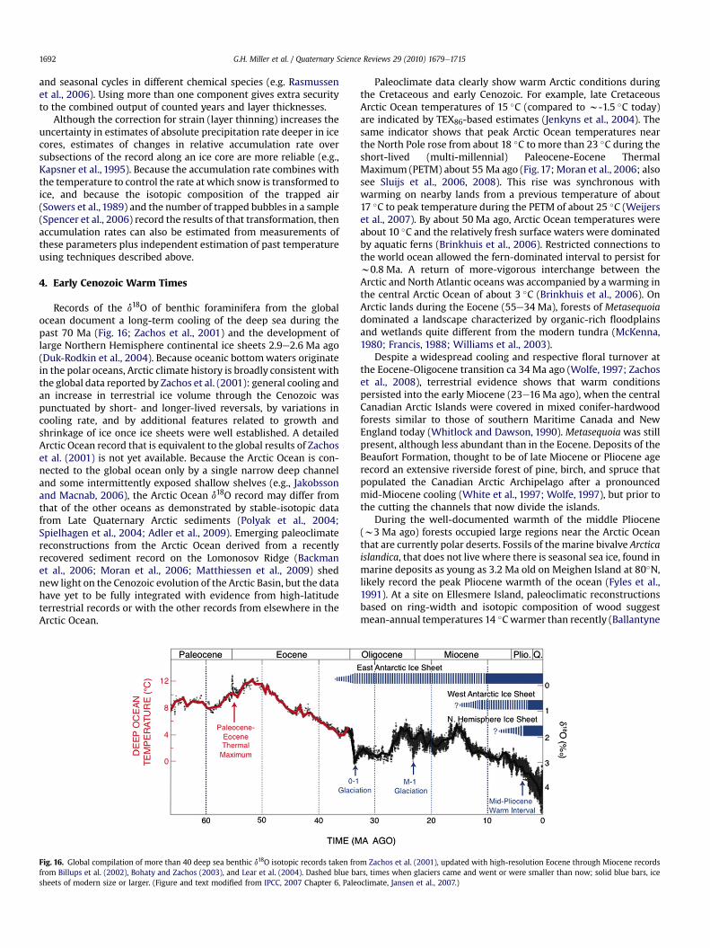
Records of the d18O of benthic foraminifera from the globalocean document a long-term cooling of the deep sea during thepast 70 Ma (Fig. 16; Zachos et al., 2001) and the development oflarge Northern Hemisphere continental ice sheets 2.9e2.6 Ma ago(Duk-Rodkin et al., 2004). Because oceanic bottomwaters originatein the polar oceans, Arctic climate history is broadly consistent withthe global data reported by Zachos et al. (2001): general cooling andan increase in terrestrial ice volume through the Cenozoic waspunctuated by short- and longer-lived reversals, by variations incooling rate, and by additional features related to growth andshrinkage of ice once ice sheets were well established. A detailedArctic Ocean record that is equivalent to the global results of Zachoset al. (2001) is not yet available. Because the Arctic Ocean is con-nected to the global ocean only by a single narrow deep channeland some intermittently exposed shallow shelves (e.g., Jakobssonand Macnab, 2006), the Arctic Ocean d18O record may differ fromthat of the other oceans as demonstrated by stable-isotopic datafrom Late Quaternary Arctic sediments (Polyak et al., 2004;Spielhagen et al., 2004; Adler et al., 2009). Emerging paleoclimatereconstructions from the Arctic Ocean derived from a recentlyrecovered sediment record on the Lomonosov Ridge (Backmanet al., 2006; Moran et al., 2006; Matthiessen et al., 2009) shednew light on the Cenozoic evolution of the Arctic Basin, but the datahave yet to be fully integrated with evidence from high-latitudeterrestrial records or with the other records from elsewhere in theArctic Ocean.
Fig. 16. Global compilation of more than 40 deep sea benthic d18O isotopic records taken frofrom Billups et al. (2002), Bohaty and Zachos (2003), and Lear et al. (2004). Dashed blue basheets of modern size or larger. (Figure and text modified from IPCC, 2007 Chapter 6, Pale
Paleoclimate data clearly show warm Arctic conditions duringthe Cretaceous and early Cenozoic. For example, late CretaceousArctic Ocean temperatures of 15 �C (compared to w-1.5 �C today)are indicated by TEX86-based estimates (Jenkyns et al., 2004). Thesame indicator shows that peak Arctic Ocean temperatures nearthe North Pole rose from about 18 �C to more than 23 �C during theshort-lived (multi-millennial) Paleocene-Eocene ThermalMaximum (PETM) about 55 Ma ago (Fig. 17; Moran et al., 2006; alsosee Sluijs et al., 2006, 2008). This rise was synchronous withwarming on nearby lands from a previous temperature of about17 �C to peak temperature during the PETM of about 25 �C (Weijerset al., 2007). By about 50 Ma ago, Arctic Ocean temperatures wereabout 10 �C and the relatively fresh surface waters were dominatedby aquatic ferns (Brinkhuis et al., 2006). Restricted connections tothe world ocean allowed the fern-dominated interval to persist forw0.8 Ma. A return of more-vigorous interchange between theArctic and North Atlantic oceans was accompanied by a warming inthe central Arctic Ocean of about 3 �C (Brinkhuis et al., 2006). OnArctic lands during the Eocene (55e34 Ma), forests of Metasequoiadominated a landscape characterized by organic-rich floodplainsand wetlands quite different from the modern tundra (McKenna,1980; Francis, 1988; Williams et al., 2003).
Despite a widespread cooling and respective floral turnover atthe Eocene-Oligocene transition ca 34 Ma ago (Wolfe, 1997; Zachoset al., 2008), terrestrial evidence shows that warm conditionspersisted into the early Miocene (23e16 Ma ago), when the centralCanadian Arctic Islands were covered in mixed conifer-hardwoodforests similar to those of southern Maritime Canada and NewEngland today (Whitlock and Dawson, 1990). Metasequoia was stillpresent, although less abundant than in the Eocene. Deposits of theBeaufort Formation, thought to be of late Miocene or Pliocene agerecord an extensive riverside forest of pine, birch, and spruce thatpopulated the Canadian Arctic Archipelago after a pronouncedmid-Miocene cooling (White et al., 1997; Wolfe, 1997), but prior tothe cutting the channels that now divide the islands.
During the well-documented warmth of the middle Pliocene(w3 Ma ago) forests occupied large regions near the Arctic Oceanthat are currently polar deserts. Fossils of the marine bivalve Arcticaislandica, that does not live where there is seasonal sea ice, found inmarine deposits as young as 3.2 Ma old on Meighen Island at 80�N,likely record the peak Pliocene warmth of the ocean (Fyles et al.,1991). At a site on Ellesmere Island, paleoclimatic reconstructionsbased on ring-width and isotopic composition of wood suggestmean-annual temperatures 14 �Cwarmer than recently (Ballantyne
m Zachos et al. (2001), updated with high-resolution Eocene through Miocene recordsrs, times when glaciers came and went or were smaller than now; solid blue bars, iceoclimate, Jansen et al., 2007.)
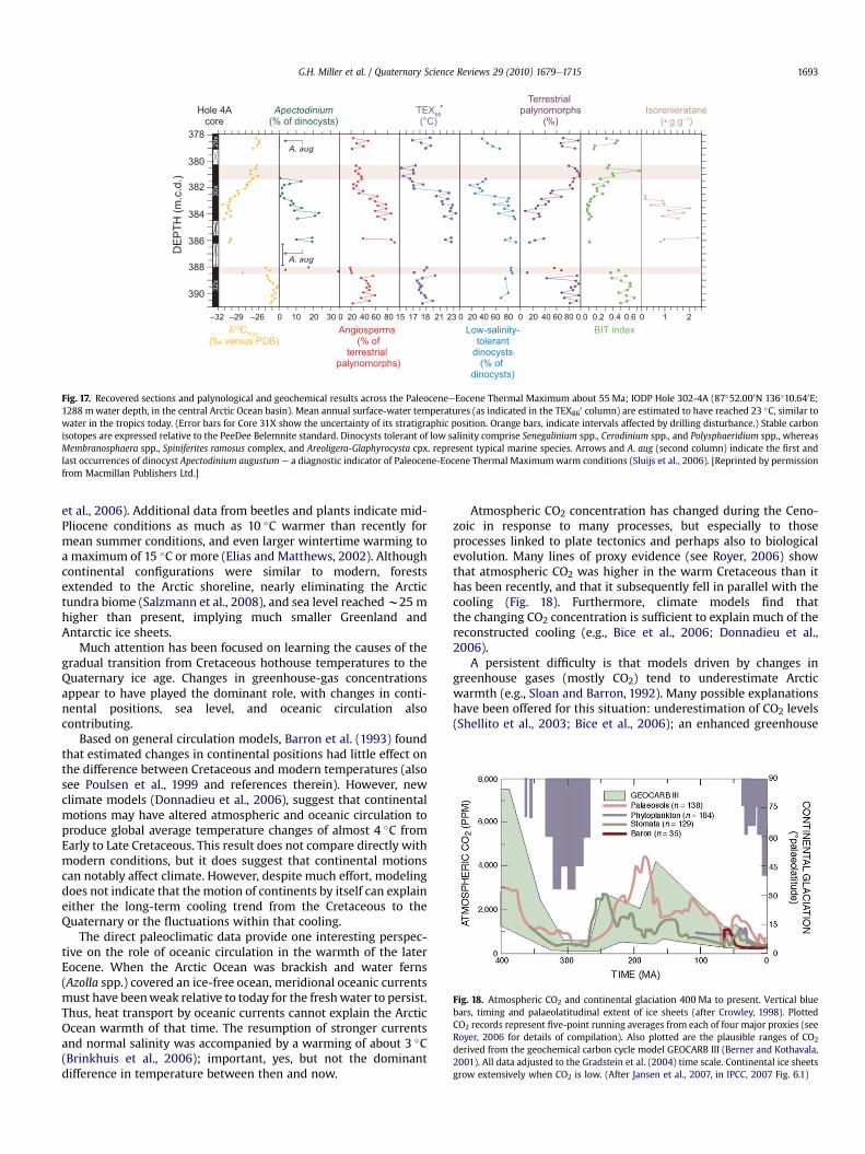
Fig. 17. Recovered sections and palynological and geochemical results across the PaleoceneeEocene Thermal Maximum about 55 Ma; IODP Hole 302-4A (87�52.000N 136�10.640E;1288 mwater depth, in the central Arctic Ocean basin). Mean annual surface-water temperatures (as indicated in the TEX86
0 column) are estimated to have reached 23 �C, similar towater in the tropics today. (Error bars for Core 31X show the uncertainty of its stratigraphic position. Orange bars, indicate intervals affected by drilling disturbance.) Stable carbonisotopes are expressed relative to the PeeDee Belemnite standard. Dinocysts tolerant of low salinity comprise Senegalinium spp., Cerodinium spp., and Polysphaeridium spp., whereasMembranosphaera spp., Spiniferites ramosus complex, and Areoligera-Glaphyrocysta cpx. represent typical marine species. Arrows and A. aug (second column) indicate the first andlast occurrences of dinocyst Apectodinium augustum e a diagnostic indicator of Paleocene-Eocene Thermal Maximumwarm conditions (Sluijs et al., 2006). [Reprinted by permissionfrom Macmillan Publishers Ltd.]
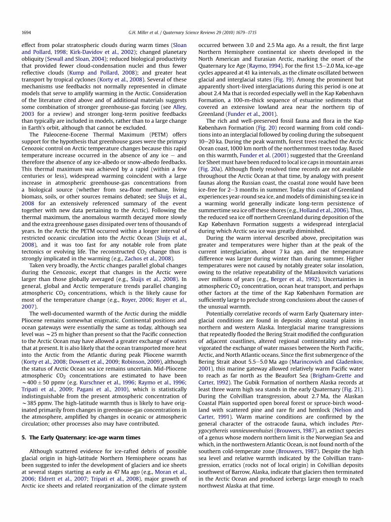
Fig. 18. Atmospheric CO2 and continental glaciation 400 Ma to present. Vertical bluebars, timing and palaeolatitudinal extent of ice sheets (after Crowley, 1998). PlottedCO2 records represent five-point running averages from each of four major proxies (seeRoyer, 2006 for details of compilation). Also plotted are the plausible ranges of CO2
derived from the geochemical carbon cycle model GEOCARB III (Berner and Kothavala,2001). All data adjusted to the Gradstein et al. (2004) time scale. Continental ice sheetsgrow extensively when CO2 is low. (After Jansen et al., 2007, in IPCC, 2007 Fig. 6.1)
G.H. Miller et al. / Quaternary Science Reviews 29 (2010) 1679e1715 1693
et al., 2006). Additional data from beetles and plants indicate mid-Pliocene conditions as much as 10 �C warmer than recently formean summer conditions, and even larger wintertime warming toa maximum of 15 �C or more (Elias and Matthews, 2002). Althoughcontinental configurations were similar to modern, forestsextended to the Arctic shoreline, nearly eliminating the Arctictundra biome (Salzmann et al., 2008), and sea level reachedw25 mhigher than present, implying much smaller Greenland andAntarctic ice sheets.
Much attention has been focused on learning the causes of thegradual transition from Cretaceous hothouse temperatures to theQuaternary ice age. Changes in greenhouse-gas concentrationsappear to have played the dominant role, with changes in conti-nental positions, sea level, and oceanic circulation alsocontributing.
Based on general circulation models, Barron et al. (1993) foundthat estimated changes in continental positions had little effect onthe difference between Cretaceous and modern temperatures (alsosee Poulsen et al., 1999 and references therein). However, newclimate models (Donnadieu et al., 2006), suggest that continentalmotions may have altered atmospheric and oceanic circulation toproduce global average temperature changes of almost 4 �C fromEarly to Late Cretaceous. This result does not compare directly withmodern conditions, but it does suggest that continental motionscan notably affect climate. However, despite much effort, modelingdoes not indicate that the motion of continents by itself can explaineither the long-term cooling trend from the Cretaceous to theQuaternary or the fluctuations within that cooling.
The direct paleoclimatic data provide one interesting perspec-tive on the role of oceanic circulation in the warmth of the laterEocene. When the Arctic Ocean was brackish and water ferns(Azolla spp.) covered an ice-free ocean, meridional oceanic currentsmust have beenweak relative to today for the freshwater to persist.Thus, heat transport by oceanic currents cannot explain the ArcticOcean warmth of that time. The resumption of stronger currentsand normal salinity was accompanied by a warming of about 3 �C(Brinkhuis et al., 2006); important, yes, but not the dominantdifference in temperature between then and now.
Atmospheric CO2 concentration has changed during the Ceno-zoic in response to many processes, but especially to thoseprocesses linked to plate tectonics and perhaps also to biologicalevolution. Many lines of proxy evidence (see Royer, 2006) showthat atmospheric CO2 was higher in the warm Cretaceous than ithas been recently, and that it subsequently fell in parallel with thecooling (Fig. 18). Furthermore, climate models find thatthe changing CO2 concentration is sufficient to explain much of thereconstructed cooling (e.g., Bice et al., 2006; Donnadieu et al.,2006).
A persistent difficulty is that models driven by changes ingreenhouse gases (mostly CO2) tend to underestimate Arcticwarmth (e.g., Sloan and Barron, 1992). Many possible explanationshave been offered for this situation: underestimation of CO2 levels(Shellito et al., 2003; Bice et al., 2006); an enhanced greenhouse
G.H. Miller et al. / Quaternary Science Reviews 29 (2010) 1679e17151694
effect from polar stratospheric clouds during warm times (Sloanand Pollard, 1998; Kirk-Davidov et al., 2002); changed planetaryobliquity (Sewall and Sloan, 2004); reduced biological productivitythat provided fewer cloud-condensation nuclei and thus fewerreflective clouds (Kump and Pollard, 2008); and greater heattransport by tropical cyclones (Korty et al., 2008). Several of thesemechanisms use feedbacks not normally represented in climatemodels that serve to amplify warming in the Arctic. Considerationof the literature cited above and of additional materials suggestssome combination of stronger greenhouse-gas forcing (see Alley,2003 for a review) and stronger long-term positive feedbacksthan typically are included in models, rather than to a large changein Earth’s orbit, although that cannot be excluded.
The Paleocene-Eocene Thermal Maximum (PETM) offerssupport for the hypothesis that greenhouse gases were the primaryCenozoic control on Arctic temperature changes because this rapidtemperature increase occurred in the absence of any ice e andtherefore the absence of any ice-albedo or snow-albedo feedbacks.This thermal maximum was achieved by a rapid (within a fewcenturies or less), widespread warming coincident with a largeincrease in atmospheric greenhouse-gas concentrations froma biological source (whether from sea-floor methane, livingbiomass, soils, or other sources remains debated; see Sluijs et al.,2008 for an extensively referenced summary of the eventtogether with new data pertaining to the Arctic). Following thethermal maximum, the anomalous warmth decayed more slowlyand the extra greenhouse gases dissipated over tens of thousands ofyears. In the Arctic the PETM occurred within a longer interval ofrestricted oceanic circulation into the Arctic Ocean (Sluijs et al.,2008), and it was too fast for any notable role from platetectonics or evolving life. The reconstructed CO2 change thus isstrongly implicated in the warming (e.g., Zachos et al., 2008).
Taken very broadly, the Arctic changes parallel global changesduring the Cenozoic, except that changes in the Arctic werelarger than those globally averaged (e.g., Sluijs et al., 2008). Ingeneral, global and Arctic temperature trends parallel changingatmospheric CO2 concentrations, which is the likely cause formost of the temperature change (e.g., Royer, 2006; Royer et al.,2007).
The well-documented warmth of the Arctic during the middlePliocene remains somewhat enigmatic. Continental positions andocean gateways were essentially the same as today, although sealevel wasw25 m higher than present so that the Pacific connectionto the Arctic Ocean may have allowed a greater exchange of watersthat at present. It is also likely that the ocean transportedmore heatinto the Arctic from the Atlantic during peak Pliocene warmth(Korty et al., 2008; Dowsett et al., 2009; Robinson, 2009), althoughthe status of Arctic Ocean sea ice remains uncertain. Mid-Plioceneatmospheric CO2 concentrations are estimated to have beenw400� 50 ppmv (e.g. Kurschner et al., 1996; Raymo et al., 1996;Tripati et al., 2009; Pagani et al., 2010), which is statisticallyindistinguishable from the present atmospheric concentration ofw385 ppmv. The high-latitude warmth thus is likely to have orig-inated primarily from changes in greenhouse-gas concentrations inthe atmosphere, amplified by changes in oceanic or atmosphericcirculation; other processes also may have contributed.
5. The Early Quaternary: ice-age warm times
Although scattered evidence for ice-rafted debris of possibleglacial origin in high-latitude Northern Hemisphere oceans hasbeen suggested to infer the development of glaciers and ice sheetsat several stages starting as early as 47 Ma ago (e.g., Moran et al.,2006; Eldrett et al., 2007; Tripati et al., 2008), major growth ofArctic ice sheets and related reorganization of the climate system
occurred between 3.0 and 2.5 Ma ago. As a result, the first largeNorthern Hemisphere continental ice sheets developed in theNorth American and Eurasian Arctic, marking the onset of theQuaternary Ice Age (Raymo, 1994). For the first 1.5e2.0 Ma, ice-agecycles appeared at 41 ka intervals, as the climate oscillated betweenglacial and interglacial states (Fig. 19). Among the prominent butapparently short-lived interglaciations during this period is one atabout 2.4 Ma that is recorded especially well in the Kap KøbenhavnFormation, a 100-m-thick sequence of estuarine sediments thatcovered an extensive lowland area near the northern tip ofGreenland (Funder et al., 2001).
The rich and well-preserved fossil fauna and flora in the KapKøbenhavn Formation (Fig. 20) record warming from cold condi-tions into an interglacial followed by cooling during the subsequent10e20 ka. During the peak warmth, forest trees reached the ArcticOcean coast, 1000 km north of the northernmost trees today. Basedon this warmth, Funder et al. (2001) suggested that the GreenlandIce Sheetmust havebeen reduced to local ice caps inmountain areas(Fig. 20a). Although finely resolved time records are not availablethroughout the Arctic Ocean at that time, by analogy with presentfaunas along the Russian coast, the coastal zone would have beenice-free for 2e3 months in summer. Today this coast of Greenlandexperiences year-round sea ice, andmodels of diminishing sea ice ina warming world generally indicate long-term persistence ofsummertime sea ice off these shores (e.g., Holland et al., 2006). Thus,the reduced sea ice off northern Greenland during deposition of theKap København Formation suggests a widespread interglacialduring which Arctic sea ice was greatly diminished.
During the warm interval described above, precipitation wasgreater and temperatures were higher than at the peak of thecurrent interglaciation, about 7 ka ago, and the temperaturedifference was larger during winter than during summer. Highertemperatures were not caused by notably greater solar insolation,owing to the relative repeatability of the Milankovitch variationsover millions of years (e.g., Berger et al., 1992). Uncertainties inatmospheric CO2 concentration, ocean heat transport, and perhapsother factors at the time of the Kap København Formation aresufficiently large to preclude strong conclusions about the causes ofthe unusual warmth.
Potentially correlative records of warm Early Quaternary inter-glacial conditions are found in deposits along coastal plains innorthern and western Alaska. Interglacial marine transgressionsthat repeatedly flooded the Bering Straitmodified the configurationof adjacent coastlines, altered regional continentality and rein-vigorated the exchange of water masses between the North Pacific,Arctic, and North Atlantic oceans. Since the first submergence of theBering Strait about 5.5e5.0 Ma ago (Marincovich and Gladenkov,2001), this marine gateway allowed relatively warm Pacific waterto reach as far north as the Beaufort Sea (Brigham-Grette andCarter, 1992). The Gubik Formation of northern Alaska records atleast three warm high sea stands in the early Quaternary (Fig. 21).During the Colvillian transgression, about 2.7 Ma, the AlaskanCoastal Plain supported open boreal forest or spruce-birch wood-land with scattered pine and rare fir and hemlock (Nelson andCarter, 1991). Warm marine conditions are confirmed by thegeneral character of the ostracode fauna, which includes Pter-ygocythereis vannieuwenhuisei (Brouwers, 1987), an extinct speciesof a genus whose modern northern limit is the Norwegian Sea andwhich, in the northwestern Atlantic Ocean, is not found north of thesouthern cold-temperate zone (Brouwers, 1987). Despite the highsea level and relative warmth indicated by the Colvillian trans-gression, erratics (rocks not of local origin) in Colvillian depositssouthwest of Barrow, Alaska, indicate that glaciers then terminatedin the Arctic Ocean and produced icebergs large enough to reachnorthwest Alaska at that time.

Fig. 19. The average isotopic composition (d18O) of bottom-dwelling foraminifera from a globally distributed set of 57 sediment cores that record the last 5.3 Ma (modified fromLisiecki and Raymo, 2005). The d18O is controlled primarily by global ice volume and deep-ocean temperature, with less ice or warmer temperatures (or both) upward in the core.The influence of Milankovitch frequencies of Earth’s orbital variation are present throughout, but glaciation increased about 2.7 Ma ago concurrently with establishment of a strong41 ka variability linked to Earth’s obliquity (changes in tilt of Earth’s spin axis), and the additional increase in glaciation about 1.2e0.7 Ma parallels a shift to stronger 100 kavariability. Dashed lines are used because the changes seem to have been gradual. The general trend toward higher d18O that runs through this series reflects the long-term drifttoward a colder Earth that began in the early Cenozoic (see Fig. 16). http://lorraine-lisiecki.com/stack.html
G.H. Miller et al. / Quaternary Science Reviews 29 (2010) 1679e1715 1695
The subsequent Bigbendian transgression (about 2.5 Ma ago),characterized by rich molluscan faunas including the gastropodLittorina squalida and the bivalve Clinocardium californiense (Carteret al., 1986), indicates renewed warmth along northern Alaska. Themodern northern limit of both of these mollusk species is well tothe south (Norton Sound, Alaska). The presence of sea otter bonessuggests that the limit of seasonal ice on the Beaufort Sea wasrestricted during the Bigbendian interval to positions north of theColville River and thus well north of typical 20th-century positions(Carter et al., 1986); modern sea otters cannot tolerate severeseasonal sea-ice conditions (Schneider and Faro, 1975).
The Fishcreekian transgression (about 2.4e2.1 Ma ago) has beencorrelated with the Kap København Formation on Greenland(Brigham-Grette and Carter, 1992). However, age control is impre-cise, and Brigham (1985) and Goodfriend et al. (1996) suggestedthat the Fishcreekian could be as young as 1.4 Ma. This depositcontains several mollusk species that currently are found onlysouth of the winter sea ice margin. Moreover, sea otter remains andthe intertidal gastropod Littorina squalida at Fish Creek suggest thatperennial sea ice was absent or severely restricted during theFishcreekian transgression (Carter et al., 1986). Correlative depositsrich in mollusk species that currently live only well to the south are
Fig. 20. (A) Greenland without ice for the last time? Dark green, boreal forest; light greentemperature gradient is constructed from a comparison between North Greenland and norassumed to retain the Holocene pattern. Topographical base, from model by Letreguilly et alKap København Formation, North Greenland. The sand was deposited in an estuary about(Figure and Photograph of by S.V. Funder.).
reported from the coastal plain at Nome, Alaska (Kaufman andBrigham-Grette, 1993).
The available data clearly indicate episodes of relatively warmconditions that correlate with high sea levels and reduced sea ice inthe early Quaternary. The high sea levels suggest the melting ofland ice. Thus the correlation of warmth with diminished ice onland and at sea is analogous to features of contemporary change, asindicated by recent instrumental observations, model results, anddata from other time intervals.
6. The Mid-Pleistocene Transition (MPT): 41 ka and 100 kaworlds
Throughout the Quaternary the cyclical waxing and waning ofcontinental ice sheets has dominated global climate variability inresponse to variations in solar insolation caused by features ofEarth’s orbit. After the onset of glaciation in North America about2.7 Ma ago (Raymo, 1994), ice grew and shrank as Earth’s obliquity(tilt) varied in its 41 ka cycle. But between 1.2 and 0.7 Ma, thevariations in ice volume became larger and slower, and anapproximately 100-ka period has dominated during the last 700 kaor so (Fig. 19). Although Earth’s eccentricity varies with an
, deciduous forest; brown, tundra and alpine heaths; white, ice caps. The north-souththwest European temperatures, using standard lapse rate; distribution of precipitation. (1991) of Greenland’s sub-ice topography after isostatic recovery. (B) Upper part of the2.4 Ma; it contains abundant well-preserved leaves, seeds, twigs, and insect remains.

Fig. 21. The largely marine Gubik Formation, North Slope of Alaska, contains three superposed lower units that record relative sea level as high þ30 to þ40 m. Pollen in thesedeposits suggests that borderland vegetation at each of these times was less forested; boreal forests or spruce-birch woodlands at 2.7 Ma gave way to larch and spruce forests atabout 2.6 Ma and to open tundra by about 2.4 Ma (see photographs by Robert Nelson, Colby College, who analyzed the pollen; oldest at top). Isotopic reference time series of Lisieckiand Raymo (2005) suggests best as assignments for these sea level events (Brigham-Grette and Carter, 1992). [Reprinted by permission Arctic Institute of North America.]
G.H. Miller et al. / Quaternary Science Reviews 29 (2010) 1679e17151696
approximately 100 ka period, this variation does not cause as muchchange in solar insolation in the key regions of ice growth as doprecession and obliquity cycles, so eccentricity in unlikely to be thecause of this change; the reason for the dominant 100 ka period inice volume remains obscure.
The MPT is of particular interest because it does not seem tohave been caused by any major change in Earth’s orbital behavior,and so the transition likely reflects a fundamental threshold withinthe climate system. Models for the 100 ka variability commonlyassign a major role to the ice sheets themselves and especially tothe Laurentide Ice Sheet, which dominated the total global changein ice volume (e.g., Marchant and Denton, 1996). Roe and Allen(1999) assessed six different explanations of this behavior andfound that all fit the data rather well; no one model has superiorityover another.
A key observation that must be satisfied in any explanation forthis change is that the ice sheets of the last 700 ka were larger involume but smaller in area thanwere earlier ice sheets (Boellstorff,1978; Balco et al., 2005a,b; Clark et al., 2006). Clark and Pollard(1998) used this observation to argue that the early LaurentideIce Sheets must have had a substantially lower surface elevationthan in the late Pleistocene, possibly by as much as 1 km. Theyargued that at the onset of the Quaternary, ice sheets advanced overeasily deformed water-saturated weathered terrain. The low basal
shear strength allowed fast ice flow, producing aerial extensive, butrelatively thin ice sheets. Successive glacial cycles gradually erodedthe regolith, eventually exposing irregular bedrock in the centralregion. With increased resistance to basal sliding, the ice sheetseventually became thicker with a steeper surface profile, but notquite as extensive aerially as the early Quaternary ice sheets,despite their greater ice volume.
Other hypotheses emphasize the gradual global cooling thatbegan in the early Cenozoic (Raymo et al., 1997, 2006; Ruddiman,2003). If, for example, the 100-ka cycle requires that the Lauren-tide Ice Sheet grow sufficiently large and thick to trap enough ofEarth’s internal heat that thaws the ice-sheet bed, then long-termcooling may have reached the threshold at which the ice sheetbecame thick enough. Marshall and Clark (2002) modeled thegrowth and decay of the Laurentide Ice Sheet and found that duringgrowth the ice was frozen to its bed, decreasing flow velocities.After many tens of thousands of years, the modeled ice had thick-ened sufficiently to trap enough geothermal heat to thaw the bed,which allowed faster flow. Faster flow of the ice sheet lowered thesurface gradient, which allowed warming and melting. Behaviorsuch as that described could cause the main variations of icevolume to be slower than the orbitally driven variations in insola-tion. Alternative hypotheses require interactions in the SouthernOcean between the ocean and sea ice and between the ocean and

G.H. Miller et al. / Quaternary Science Reviews 29 (2010) 1679e1715 1697
the atmosphere (Gildor et al., 2002). For example, Toggweiler(2008) suggested that because of the close connection betweenthe southern westerly winds and meridional overturning circula-tion in the Southern Ocean, shifts in wind fields could control theexchange of CO2 between the ocean and the atmosphere. Carbonmodels support the notion that weathering and the burial ofcarbonate can be perturbed in ways that alter deep ocean carbonstorage and result in 100 ka CO2 cycles. Others have suggested that100 ka cycles and CO2might be controlled by variability in obliquitycycles (i.e., two or three 41 ka cycles Huybers, 2006) or by variableprecession cycles (altering the 19 ka and 23 ka cycles; Raymo,1997). Ruddiman (2006) recently furthered these ideas but sug-gested that since 900 ka ago, CO2-amplified ice growth continuedat the 41 ka intervals but that polar cooling dampened ice ablation.His CO2-feedback hypothesis suggests a mechanism that combinesthe control of 100 ka cycles with precession cycles (19 ka and 23 ka)and with tilt cycles (41 ka).
Other hypotheses also exist for these changes. A completeexplanation of the onset of extensive glaciation on North Americaand Eurasia as well as Greenland about 2.8 Ma ago, or of the tran-sition from 41 ka to 100 ka ice-age cycles, remains the object ofongoing investigations.
7. A link between ice volume, air temperature andgreenhouse gases
The globally averaged temperature decrease during the 100-kaice-age cycles was about 5e6 �C (Jansen et al., 2007). Largerdecreases are calculated for the Arctic and close to the ice sheets,with a decrease of w22 �C atop the Greenland Ice Sheet at the lastglacial maximum (Cuffey et al., 1995). The total change in solarradiation reaching the planet during these cycles was near zero, butorbital features served primarily to change insolation seasonallyand geographically.
Many factors probably contributed to this large temperaturechange despite the small global change in total insolation (Jansenet al., 2007). Cooling produced growth of reflective ice thatincreased the planetary albedo, while the great height of the icesheets on its own reduced Arctic temperatures as well. Complexchanges, especially in the ocean, reduced atmospheric carbondioxide concentrations, and both oceanic and terrestrial changesreduced atmospheric water vapor, methane and nitrous oxide, allof which are greenhouse gases; changes in water vapor and carbondioxide were most important. Increasing aridity in some areas andglacial outwash in others produced additional dust that reducedthe flux of insolation reaching the planet’s surface (e.g., Mahowaldet al., 2006). Cooling caused regions formerly forested to give wayto grasslands, tundra or dune fields, further increasing theplanetary albedo. While Earth’s orbital features paced the ice-age cycles, strong positive feedbacks are required to providequantitatively accurate explanations of the observed glacial andinterglacial changes.
The relation between climate and carbon dioxide has beenstrongly correlated for at least the past 800 ka (Siegenthaler et al.,2005, Fig. 22, Lüthi et al., 2008), and the growth and shrinkage ofice, cooling and warming of the globe, and other changes haverepeated along similar, although not identical paths. Differencesbetween some successive cycles that are of interest are discussednext.
8. Marine Isotopic Stage 11 e a long interglaciation
Following the mid-Pleistocene transition, the growth and decayof ice sheets followed a 100 ka cycle: brief, warm interglaciationslasted 10 to about 40 ka, after which ice progressively increased in
volume to a maximum, before ice volumes decreased rapidly andthe planet transitioned into the next interglaciation (e.g., Kellogg,1977; Ruddiman et al., 1986; Jansen et al., 1988; Heinrich andBaumann, 1994; Bauch and Erlenkeuser, 2003). As discussedabove, this 100 ka cycle is unlikely to be linked to the changes in theeccentricity of Earth’s orbit about the Sun because the 100 kaeccentricity cycle produces so little change in solar isolationreaching the Earth.
The eccentricity exhibits an additional cycle ofw400 ka; Earth’sorbit goes from almost round to more eccentric to almost round inabout 100 ka, but the maximum eccentricity reached in these 100-ka cycles increases and decreases within a 400-ka cycle (Berger andLoutre,1991; Loutre, 2003).When the orbit is almost round, there islittle effect from Earth’s precession. But, about 400 ka ago, duringmarine isotope stage (MIS) 11, the 400-ka cycle caused a nearlyround orbit to persist. The MIS 11 interglaciation lasted longer thanprevious or subsequent interglaciations (see Droxler et al., 2003and references therein; Kandiano and Bauch, 2007; Jouzel et al.,2007), perhaps because the summer insolation at high northernlatitudes did not become low enough at the end of the first 10 kaprecession hemicycle to allow ice growth in the Arctic. WhenEarth’s orbit is nearly round, there is little change in insolationduring a precession cycle (Fig. 23).
Mid- and low-latitude paleoclimate records show that MIS 11lasted w30 ka, rather than the typical 10 ka duration, but sedi-ments containing MIS 11 are rare in the Arctic (cf. Kaufman andBrigham-Grette, 1993) and their temperature signals are incon-clusive (see Stanton-Frazee et al., 1999; Bauch et al., 2000; Droxlerand Farrell, 2000; Helmke and Bauch, 2003). Sea level during MIS11 was higher than at any time since (cf. Olson and Hearty, 2009),and data from Greenland are consistent with notable shrinkage orloss of the ice sheet accompanying the long warmth, although thedating is poorly constrained (Willerslev et al., 2007).
9. Marine Isotopic Stage 5e: The Last Interglaciation
The warmest millennia of at least the past 250,000 yearsoccurred during MIS 5, and especially during the warmest part ofthat interglaciation, MIS 5e (McManus et al., 1994; Fronval andJansen, 1997; Bauch et al., 1999; Kukla, 2000). At that time globalice volumes were smaller than they are today, and Earth’s orbitalparameters aligned to produce a strong positive anomaly in solarradiation during summer throughout the Northern Hemisphere(Berger and Loutre, 1991). Between 130 and 127 ka, the averagesolar radiation during the key summermonths (May, June, and July)was about 11% greater than solar radiation at present throughoutthe Northern Hemisphere, and a slightly greater anomaly, 13%,existed over the Arctic. Greater solar energy in summer, melting ofthe large Northern Hemisphere ice sheets, and intensification of theNorth Atlantic Drift (Chapman et al., 2000; Bauch and Kandiano,2007) combined to reduce Arctic Ocean sea ice, allow expansionof boreal forest to the Arctic Ocean shore throughout large regions,reduce permafrost, and melt almost all glaciers in the NorthernHemisphere (CAPE Last Interglacial Project Members, 2006).
High solar radiation in summer during MIS 5e, amplified by keyboundary-condition feedbacks (especially sea ice, seasonal snowcover, and atmospheric water vapor), collectively producedsummer temperature anomalies 4e5 �C above present over mostArctic lands (CAPE Last Interglacial Project Members, 2006),substantially above the average Northern Hemisphere summertemperature anomaly (1�1 �C above present; CLIMAP ProjectMembers, 1984; Bauch and Erlenkeuser, 2003). MIS 5e demon-strates the strength of positive feedbacks on Arctic warming (CAPELast Interglacial Project Members, 2006; Otto-Bliesner et al., 2006).

180
200
220
240
260
280
300O
C2
).v.m.p.p(
8007006005004003002001000Age (kyr BP)
–12
–8
–4
0
4 )C°(
ylamona
erutarepmeT
15.515.1 17 19
20
181614
13
11
10
9
8
7
6
5
3
MIS 2
Holocene
4 12
TI TII TIII TIV TV TVI TVII TVIII TIX
Fig. 22. Compilation of CO2 records and EPICA Dome C temperature anomaly over the past 800 ka from Lüthi et al. (2008). The Dome C temperature anomaly record with respect tothe mean temperature of the last millennium (based on original deuterium data interpolated to a 500-year resolution), plotted on the EDC3 timescale, is given as a black step curve.Data for CO2 are from Dome C (solid circles in purple, blue, black: this work, measured at Bern; red open circles: this work, measured at Grenoble), Taylor Dome (brown) and Vostok(green). All CO2 values are on the EDC3_gas_a age scale. Horizontal lines are the mean values of temperature and CO2 for the time periods 799e650, 650e450, 450e270 and270e50 ka BP. Glacial terminations are indicated using Roman numerals in subscript (for example TI); Marine Isotope Stages (MIS) are given in italic Arabic numerals. [Copyright2008, reprinted with permission from Nature Publishing Group]
G.H. Miller et al. / Quaternary Science Reviews 29 (2010) 1679e17151698
9.1. Terrestrial MIS 5e records
Summers throughout the Arctic were warmer during MIS 5ethan at present, but the magnitude of warming differed spatially(Fig. 24). Positive summer temperature anomalies were largestaround the Atlantic sector, where summer warming was typically4e6 �C. This anomaly extended into Siberia, but it decreased fromSiberia westward to the European sector (0e2 �C), and eastwardtoward Beringia (2e4 �C). The Arctic coast of Alaska had sea-surfacetemperatures 3 �C above recent values and considerably lesssummer sea ice than recently, but much of interior Alaska hadsmaller anomalies (0e2 �C) that probably extended into westernCanada. In contrast, northeastern Canada and parts of Greenlandhad summer temperature anomalies of about 5 �C, and perhapsmore. A stratified lacustrine sequence from the eastern CanadianArctic the captures the penultimate interglacial, as well as MIS 5eand the Holocene suggests that for at least this portion of the Arctic,only full interglacials were warm enough for lakes to be ice-free insummers long enough for the preservation of biotic-bearing sedi-ment; the record also suggested that 20th Century warmingrepresents a no-analogue situation for the lake (Axford et al., 2009).
Precipitation and winter temperatures are more difficult toreconstruct for MIS 5e than are summer temperatures. In north-eastern Europe, the latter part of MIS 5e was characterized bya marked increase in winter temperatures. A large positive wintertemperature anomaly also occurred in Russia and western Siberia,although the timing is not as well constrained (Troitsky, 1964;Gudina et al., 1983; Funder et al., 2002). Qualitative precipitationestimates for most other sectors indicate wetter conditions than inthe Holocene.
9.2. Marine MIS 5e records
Low sedimentation rates in the central Arctic Ocean and the rarepreservation of carbonate fossils limit the number of sites at whichMIS 5e can be reliably identified in sediment cores. Peak concen-trations of a foraminifer species that usually dwells in subpolarwaters were found in MIS 5e zones and interpreted to indicaterelatively warm interglacial conditions and much reduced sea-ice
cover in the interior Arctic Ocean (Nørgaard-Pedersen et al., 2007a,b; Adler et al., 2009). Interpretation of these and other proxies iscomplicated by the strong vertical stratification in the Arctic Ocean;today, warm Atlantic water (>1 �C) is in most areas isolated fromthe atmosphere by a relatively thin layer of cold (<-1 �C) low-salinity surface layer, limiting the transfer of heat to the atmo-sphere. It is not always possible to determine whether subpolarforaminifera found in Arctic Ocean sediment cores lived in warmwaters that remained isolated from the atmosphere below the coldsurface layer, or whether thewarmAtlantic water had displaced thecold surface layer and was interacting with the atmosphere andaffecting its energy balance.
Landforms and fossils from the western Arctic and Bering Straitindicate vastly reduced sea ice during MIS 5 (Fig. 25). The wintersea-ice limit is estimated to have been as much as 800 km farthernorth than its average 20th-century position, and summer sea icewas likely to have been much reduced relative to present(Brigham-Grette and Hopkins, 1995). These reconstructions areconsistent with the northward migration of treeline by hundredsof kilometers throughout much of Alaska and the expansion oftreeline to the Arctic Ocean coast in the Far East of Russia (Lozhkinand Anderson, 1995).
10. Marine Isotopic Stage 3 Warm Intervals
The Arctic temperature and precipitation history through MIS 3(about 70e30 ka ago) is difficult to reconstruct because of thepaucity of continuous records and the difficulty in providinga secure time frame. The d18O record of temperature change overthe Greenland Ice Sheet and other ice-core data show that theNorth Atlantic region experienced repeated episodes of rapid, high-magnitude climate change, when temperatures rapidly increasedby as much as 15 �C (reviewed by Alley, 2007 and referencestherein), and that eachwarm period lasted several hundred to a fewthousand years. These brief climate excursions are found not onlyin the Greenland Ice Sheet but are also recorded in cave sedimentsin China and Yemen (Wang et al., 2001; Burns et al., 2003; Dykoskiet al., 2005), in high-resolution marine records off California (Behland Kennett, 1996), and sediment cores from the Cariaco Basin

Fig. 23. Glacial cycles of the past 800 ka derived from marine-sediment and ice cores (McManus, 2004). The history of deep-ocean temperatures and global ice volume inferredfrom d18O measured in bottom-dwelling foraminifera shells preserved in Atlantic Ocean sediments. Air temperatures over Antarctica inferred from the ratio of deuterium tohydrogen in ice from central Antarctica (EPICA, 2004). Marine isotope stage 11 (MIS 11) is an interglacial whose orbital parameters were similar to those of the Holocene, yet it lastedabout twice as long as most interglacials. Note the smaller magnitude and less-pronounced interglacial warmth of the glacial cycles that preceded MIS 11. Interglaciations older thanMIS 11 were less warm than subsequent integlaciations. [Reprinted by permission from Macmillan Publishers Ltd.]
G.H. Miller et al. / Quaternary Science Reviews 29 (2010) 1679e1715 1699
(Hughen et al., 1996.), the Arabian Sea (Schulz et al., 1998) and theSea of Okhotsk (Nürnberg and Tiedemann, 2004), among manyother sites. Proxies in Greenland ice cores reflect climate change indistant as well as local regions. For example, most of the methanetrapped in ice-core bubbles was produced in tropical wetlands;none was produced on Greenland (Severinghaus et al., 1998). Theseice-core records demonstrate clearly that climate changes werebroadly synchronous across wide areas, and that the timing of thesechanges agrees within the stated uncertainties. Rapid climatechanges within MIS 3 were thus hemispheric to global in nature(see review by Alley, 2007) and are considered a sign of large-scalecoupling between the crysophere, ocean, and atmosphere (Bard,2002). The cause of these events is still debated. However,Broecker and Hemming (2001) and Bard (2002) among otherssuggested that they were likely the result of major and abruptreorganizations of the ocean’s thermohaline circulation, probablyrelated to ice sheet instabilities that introduced large quantities offresh water and icebergs into the North Atlantic (Alley, 2007). Such
large and abrupt oscillations were linked to changes in NorthAtlantic surface conditions and probably to large-scale oceaniccirculation. Such abrupt changes, persisted into the Holocene (MIS1), although still linked to an ice-age cause. The youngest was onlyabout 8.2 ka ago when a large lake dammed by the receding Lau-rentide Ice Sheet flooded catastrophically when the ice-dam failed(Barber et al., 1999; Alley and Ágústsdóttir, 2005).
DuringMIS 3 ice sheets were somewhat reduced comparedwithice volumes during MIS 2 and MIS 4, and sea level was slightlyhigher, but the coastline was still well offshore in most places, andthe increased continentality very likely contributed to relativelyhigh summer temperatures that presumably were offset by colderwinters. For example, on the New Siberian Islands in the EastSiberian Sea, Andreev et al. (2001) documented the existence ofgraminoid-rich tundra covering wide areas of the emergent shelfduring MIS 3, with summer temperatures possibly 2 �C higher thanduring the 20th century. At Elikchan 4 Lake in the upper Kolymadrainage, the sediment record contains at least three MIS 3
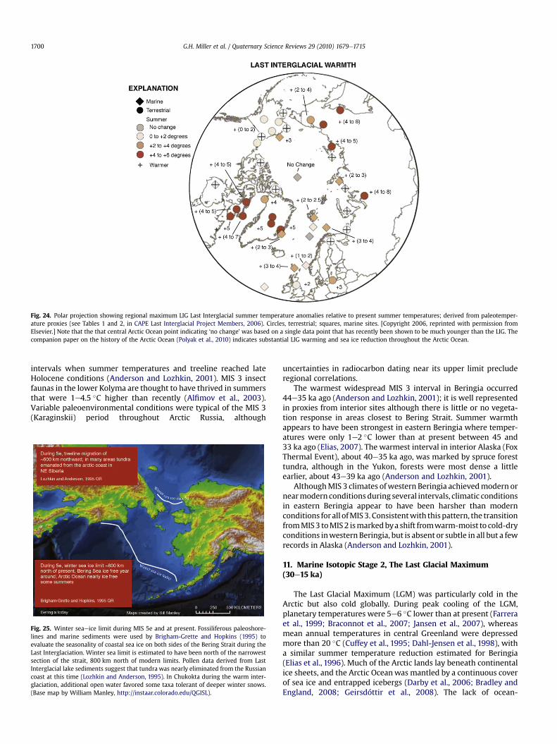
Fig. 24. Polar projection showing regional maximum LIG Last Interglacial summer temperature anomalies relative to present summer temperatures; derived from paleotemper-ature proxies (see Tables 1 and 2, in CAPE Last Interglacial Project Members, 2006). Circles, terrestrial; squares, marine sites. [Copyright 2006, reprinted with permission fromElsevier.] Note that the that central Arctic Ocean point indicating ‘no change’ was based on a single data point that has recently been shown to be much younger than the LIG. Thecompanion paper on the history of the Arctic Ocean (Polyak et al., 2010) indicates substantial LIG warming and sea ice reduction throughout the Arctic Ocean.
G.H. Miller et al. / Quaternary Science Reviews 29 (2010) 1679e17151700
intervals when summer temperatures and treeline reached lateHolocene conditions (Anderson and Lozhkin, 2001). MIS 3 insectfaunas in the lower Kolyma are thought to have thrived in summersthat were 1e4.5 �C higher than recently (Alfimov et al., 2003).Variable paleoenvironmental conditions were typical of the MIS 3(Karaginskii) period throughout Arctic Russia, although
Fig. 25. Winter seaeice limit during MIS 5e and at present. Fossiliferous paleoshore-lines and marine sediments were used by Brigham-Grette and Hopkins (1995) toevaluate the seasonality of coastal sea ice on both sides of the Bering Strait during theLast Interglaciation. Winter sea limit is estimated to have been north of the narrowestsection of the strait, 800 km north of modern limits. Pollen data derived from LastInterglacial lake sediments suggest that tundra was nearly eliminated from the Russiancoast at this time (Lozhkin and Anderson, 1995). In Chukokta during the warm inter-glaciation, additional open water favored some taxa tolerant of deeper winter snows.(Base map by William Manley, http://instaar.colorado.edu/QGISL).
uncertainties in radiocarbon dating near its upper limit precluderegional correlations.
The warmest widespread MIS 3 interval in Beringia occurred44e35 ka ago (Anderson and Lozhkin, 2001); it is well representedin proxies from interior sites although there is little or no vegeta-tion response in areas closest to Bering Strait. Summer warmthappears to have been strongest in eastern Beringia where temper-atures were only 1e2 �C lower than at present between 45 and33 ka ago (Elias, 2007). The warmest interval in interior Alaska (FoxThermal Event), about 40e35 ka ago, was marked by spruce foresttundra, although in the Yukon, forests were most dense a littleearlier, about 43e39 ka ago (Anderson and Lozhkin, 2001).
AlthoughMIS 3 climates ofwestern Beringia achievedmodern ornearmodern conditions during several intervals, climatic conditionsin eastern Beringia appear to have been harsher than modernconditions forall ofMIS3. Consistentwith thispattern, the transitionfromMIS3 toMIS2 ismarkedbya shift fromwarm-moist to cold-dryconditions inwesternBeringia, but is absent or subtle in all but a fewrecords in Alaska (Anderson and Lozhkin, 2001).
11. Marine Isotopic Stage 2, The Last Glacial Maximum(30e15 ka)
The Last Glacial Maximum (LGM) was particularly cold in theArctic but also cold globally. During peak cooling of the LGM,planetary temperatures were 5e6 �C lower than at present (Farreraet al., 1999; Braconnot et al., 2007; Jansen et al., 2007), whereasmean annual temperatures in central Greenland were depressedmore than 20 �C (Cuffey et al., 1995; Dahl-Jensen et al., 1998), witha similar summer temperature reduction estimated for Beringia(Elias et al., 1996). Much of the Arctic lands lay beneath continentalice sheets, and the Arctic Oceanwas mantled by a continuous coverof sea ice and entrapped icebergs (Darby et al., 2006; Bradley andEngland, 2008; Geirsdóttir et al., 2008). The lack of ocean-

G.H. Miller et al. / Quaternary Science Reviews 29 (2010) 1679e1715 1701
atmosphere transfer of heat during winter months would result inexceptionally cold winters, not only over the Arctic Ocean proper,but also across adjacent lands. These factors together limit thedirect records of LGM climate across most of the Arctic. The avail-able evidence for terrestrial ecosystems suggests that low- andhigh-shrub tundra were extremely restricted during the LGM, andlargely replaced by polar desert or graminoid and forb tundra andan intergradation of steppe and tundra in the north Eurasianinterior (Bigelow et al., 2003), ecosystem changes consistent withcold, dry climates with little snow cover.
Global ice volumes peaked about 21 ka ago. Rising solar inso-lation across the Northern Hemisphere in summer due to orbitalfeatures and rising greenhouse gases caused Northern Hemisphereice sheets to begin to recede from near their maxima shortly after20 ka ago, with the rate of recession increasing noticeably afterabout 16 ka ago (see, e.g., Alley et al., 2002; Dyke et al., 2003; Clarket al., 2004). Most coastlines became ice-free before 12 ka ago, andice continued to melt rapidly as summer insolation reached a peak(about 9% above modern insolation) about 11 ka ago. An extensiveliterature addresses the patterns of deglaciation, and for the NorthAtlantic in particular, the climatic fluctuations that occurred withinthe deglacial period.
12. Marine Isotopic Stage 1, The Holocene
The transition fromMIS 2 to MIS 1, which marks the start of theHolocene, is commonly placed at the abrupt termination of theYounger Dryas cold event, about 11.7 ka ago (Rasmussen et al.,2006). By 6 ka ago, sea level and ice volumes were close to thoseobserved more recently, and greenhouse gases in the atmospherediffered little from pre-industrial conditions (e.g., Jansen et al.,2007). A wide variety of evidence from terrestrial and marinearchives indicates that peak MIS 1 Arctic summertime warmth wasachieved during the early Holocene, when most regions of theArctic experienced sustained summer temperatures that exceededobserved 20th century values. This period of peak warmth, which is
Fig. 26. The Arctic Holocene Thermal Maximum. Items compared, top to bottom: seasonaltemperature from the GISP2 drilling project (Taylor et al., 1997; Alley, 2000); age distributtreeline (MacDonald et al., 2008); and the frequency of Western Arctic sites that experienc
geographically variable in its timing (Kaufman et al., 2004), isgenerally referred to as the Holocene Thermal Maximum (HTM).The ultimate driver of the warming was orbital forcing, whichproduced increased summer solar radiation across the NorthernHemisphere. At 70 �N June insolation about 4 ka was about 15Wm�2 larger than present, and June insolation 11 ka ago was about45Wm�2 larger than present, for a total change of about 9% (Fig. 26;Berger and Loutre, 1991). January insolation did not change becausethere is no insolation that far north in January.
High-resolution (decades to centuries) archives containingmultiple climate proxies are available for most of the Holocenethroughout the Arctic. Consequently, the Holocene record allowsevaluation of the range of natural climate variability and of themagnitude of climate change in response to relatively smallchanges in forcings.
12.1. Holocene Thermal Maximum
Most Arctic paleoenvironmental records for the HTM recordprimarily summer temperatures. Many different proxies have beenexploited to derive these reconstructions, including biologicalproxies such as pollen, diatoms, chironomids, dinoflagellate cysts,and other microfossils; elemental and isotopic geochemical indicesfrom lacustrine and marine sediments, and ice cores; boreholetemperatures; age distributions of radiocarbon-dated tree stumpsnorth of (or above) current treeline, and the distributions of ther-mophilous marine mollusks and whales (Fig. 27).
A recent synthesis of 140 Arctic paleoclimatic and paleoenvir-onmental records extending from Beringia westward to Iceland(Kaufman et al., 2004) outlines the nature of the HTM in thewestern Arctic (Fig. 28a). Of the sites included in the synthesis 85%contain evidence of the HTM, with an average duration of 2.1 ka inBeringia to 3.5 ka in Greenland. The interval from 10 to 4 ka agocontains the greatest number of sites recording HTM conditionsand the greatest spatial extent of those conditions in the westernArctic (Fig. 28c). The HTM thermal maximum began first in
insolation patterns at 70�N (Berger and Loutre, 1991), and reconstructed Greenland airion of radiocarbon-dated fossil remains of various tree genera from north of presented Holocene Thermal Maximum conditions (Kaufman et al., 2004).

G.H. Miller et al. / Quaternary Science Reviews 29 (2010) 1679e17151702
Beringia, where warmer-than-present summers became estab-lished 14e13 ka ago. Intermediate ages for HTM initiation (10e8 kaago) are apparent in the Canadian Arctic Archipelago and in centralGreenland. The HTM on Iceland occurred a bit later, 8e6 ka ago,whereas the onset on Svalbard was earlier, by 10.8 ka ago(Svendsen and Mangerud, 1997). The latest general HTM onset(7e4 ka ago) was in the continental portions of central and easternCanada (Fig. 28b). Similarly, the earliest termination of the HTMoccurred in Beringia. Most regions registered summer cooling by5 ka ago. The average summer temperature anomaly during theHTM across the western Arctic was 1.65 �C, although they rangedfrom 0.5 to 3.0 �C, with the largest changes in the North Atlanticsector and the smallest over North Pacific sector.
Much of the pattern of the onset of the HTM can be explained inpart by regional proximity to the continental ice sheets, whichdepressed temperatures nearby until the ice melted back, and tochanges in freshwater delivery to the North Atlantic. Milankovitchcycling has also been suggested to explain the spatial variability ofthe Holocene Thermal Maximum (Maximova and Romanovsky,1988).
Records for sea-ice conditions in the Arctic Ocean and adjacentchannels have been developed by radiocarbon-dating indicatorsincluding the remains of open-water proxies such as whales and
Fig. 27. Arctic temperature reconstructions. Upper panel: Holocene summer melting on thecore section that contains evidence of melting (from Koerner and Fisher, 1990). Middle pane14C- dated sub-fossil pine wood samples (Pinus sylvestris L.) in the Scandes Mountains, centrupper limit of pine growth is indicated by the dashed line. Changes in temperature estimatecollected by L. Kullman and by G. and J. Lundqvist). Lower panel: Paleotemperature reconstfrom a cave atMo i Rana, northern Norway. Growth ceased around A.D. 1750 (from Lauritzenvalues for each variable. Figure from Bradley (2000). [Copyright 2000, reproduced with pe
walrus, warm-water marine mollusks, changes in the microfaunapreserved in marine sediments, and more recently in biomarkersdiagnostic of sea-ice or sea-ice-free organisms (see Polyak et al.,2010, for a complete treatment of the history of Arctic Ocean seaice). These reconstructions parallel the terrestrial record for themost part. They demonstrate that an increased mass of warmAtlantic water moved into the Arctic Ocean at about the beginningof the Holocene. Dates on the first appearance of the obligateAtlantic water taxon Mytilus edulis on northern Svalbard are ca10.6 ka (Salvigsen et al., 1992; Salvigsen, 2002), with peak pene-tration of Atlantic water reflected the occurrence of Modiolismodiolis by ca 9.3 ka and a strong Atlantic water presence in theArctic Ocean until 8 ka (Salvigsen, 2002). Most thermophilousmollusks disappear from Svalbard by about 5 ka, about the sametime that the first evidence of Neoglaciation appears around thenorthern North Atlantic. Dates on the flooding of Bering Strait rangefrom w12 ka ago (Keigwin et al., 2006) to slightly before 13 ka ago(England and Furze, 2008), although precise dating remainsdependent on knowledge of the marine reservoir age at that time.The influx of Pacific water to the Arctic Ocean peaked about 9e5 ka,then diminishing through the late Holocene. The extra ocean heatfrom both Atlantic and Pacific sources, coupled with increasedsummer insolation, decreased the area of perennial sea-ice cover
Agassiz Ice Cap, northern Ellesmere Island, Canada. “Melt” indicates the fraction of eachl: Estimated summer temperature anomalies in central Sweden. Black bars, elevation ofal Sweden, relative to temperatures at the modern pine limit in the region. Dashed line,d by assuming a lapse rate of 6 �C km�1 (from Dahl and Nesje, 1996, based on samplesruction from oxygen isotopes in calcite sampled along the growth axis of a stalagmite1996; Lauritzen and Lundberg 1999). Horizontal lines indicate the average 20th Centuryrmission from Elsevier.]

Fig. 28. The timing of initiation and termination of the Holocene Thermal Maximum in the western Arctic (Kaufman et al., 2004). (A) Regions reviewed in Kaufman et al., 2004. (B)Initiation of the Holocene Thermal Maximum in the western Arctic. Longitudinal distribution (left) and frequency distribution (right). (C) Spatial-temporal pattern of the HoloceneThermal Maximum in the western Arctic. Upper panel, initiation; lower panel, termination. Dot colors bracket ages of the Holocene Thermal Maximum; ages contoured using thesame color scheme. Gray dots, equivocal evidence for the Holocene Thermal Maximum. [Copyright 2004, reprinted with permission from Elsevier.]
G.H. Miller et al. / Quaternary Science Reviews 29 (2010) 1679e1715 1703
during the early Holocene. Decreased sea-ice cover in the westernArctic during the early Holocene also may be indicated by changesin concentrations of sea-salt sodium in the Penny Ice Cap (easternCanadian Arctic; Fisher et al., 1998) and the Greenland Ice Sheet(Mayewski et al., 1997). In most regions, perennial sea ice increasedin the late Holocene, although it has been suggested that sea icedeclined in the Chukchi Sea (de Vernal et al., 2005), possibly inresponse to changing rates of Atlantic water inflow in Fram Strait.
As summer temperatures increased through the early Holocene,North American treeline expanded northward into regionsformerly mantled by tundra, although the northward extentappears to have been limited to perhaps a few tens of kilometersbeyond its recent position (Seppä et al., 2003; Gajewski andMacDonald, 2004). In contrast, some treeline species expandedwell beyond their current limits in the Eurasian Arctic. Datedmacrofossils indicate that individuals of the tree genera Betula(birch) and Larix (larch) lived far north of the modern treelineacross most of northern Eurasia between 11 and 10 ka ago(Kremenetski et al., 1998; MacDonald et al., 2000a,b, 2008), andLarix extended beyond its modern limits as early 13e12 ka ago ineastern Siberia (Binney et al., 2009). In the Taimyr Peninsula ofSiberia and nearby regions the most northerly limit reached bytrees during the Holocene was more than 200 km north of thecurrent treeline (Fig. 29). Spruce (Picea) advanced slightly later thanthe other two genera. Interestingly, pine (Pinus), which now formsthe conifer treeline in Fennoscandinavia and the Kola Peninsula ofRussia, does not appear to have established appreciable forest coverat or beyond the present treeline in the Kola Peninsula until around7 ka ago (MacDonald et al., 2000a). However, quantitative recon-structions of temperature suggest that summer temperatures wereabove modern by 9 ka ago (Seppä and Birks, 2001, 2002;Hammarlund et al., 2002; Solovieva et al., 2005), and the devel-opment of extensive pine cover at and north of the present treelineappears to have been delayed relative to this warming. Treelinebegan to retreat southward across northern Eurasia 3-4 ka ago(Binney et al., 2009).
The timing of the HTM in the Eurasian Arctic overlaps thewidestexpression of the HTM in the western Arctic (Fig. 28), but it differsin two respects. The timing of onset and termination in Eurasiashows much less variability than in North America, and themagnitude of the treeline expansion and retreat is far greater in theEurasian Arctic. Fossil pollen and other indicators of vegetation ortemperature from the northern Eurasian margin also support thecontention of a prolonged warming and northern extension oftreeline during the early and middle Holocene (Fig. 28; Hyvärinen,1976; Seppä, 1996; Clayden et al., 1997; Velichko et al., 1997;
Kaakinen and Eronen, 2000; Pisaric et al., 2001; Seppä and Birks,2001, 2002; Gervais et al., 2002; Hammarlund et al., 2002;Solovieva et al., 2005).
Changes in landforms suggest that permafrost in Siberiadegraded during the HTM. A synthesis of Russian data by Astakhov(1995) indicates that melting permafrost was apparent north of theArctic Circle only in the European North, not in Siberia. In theSiberian North, permafrost partially thawed only locally, andthawing was almost entirely confined to areas under thermokarstlakes that actively formed there during the HTM. Areas south of theArctic Circle appear to have experienced deep thawing (100e200 mdepth) through the HTM, followed by renewed permafrost expan-sion after 3 ka. The deep thawing and subsequent renewal ofsurface permafrost in these regions produced an extensive thawedlayer sandwiched between shallow (20e80 m deep) more recentlyfrozen ground and deeper Pleistocene permafrost throughoutmuch of northwestern Siberia.
Quantitative estimates of HTM summer temperature anoma-lies along the northern margins of Eurasia and adjacent islandsrange from 1 to 3 �C. The geographic position of northern treelineacross Eurasia is largely controlled by summer temperature andthe length of the growing season (MacDonald et al., 2008), and insome areas the magnitude of treeline displacement theresuggests a summer warming equivalent of 2.5e7.0 �C (see forexample Birks, 1991; Wohlfarth et al., 1995; MacDonald et al.,2000a; Seppä and Birks, 2001, 2002; Hammarlund et al., 2002;Solovieva et al., 2005). Sea-surface temperature anomaliesduring the HTM were as much as 4e5 �C for the eastern NorthAtlantic sector and adjacent Arctic Ocean (Salvigsen et al., 1992;Koç et al., 1993). HTM Summer temperature anomalies in thewestern Arctic ranged from 0.5 to 3 �C, with the largest anoma-lies in the North Atlantic sector (Kerwin et al., 1999; Kaufmanet al., 2004; Flowers et al., 2008).
12.2. Neoglaciation
Many climate proxies are available to characterize the overallpattern of Late Holocene climate change. Following the HTM, mostproxy summer temperature records from the Arctic indicate anoverall cooling trend through the late Holocene. Cooling is firstrecognized between 6 and 3 ka ago, depending on the threshold forchange of each particular proxy. Records that exhibit a shift by6e5 ka ago typically also reflect intensified summer cooling about3 ka (Fig. 27).
Mostmountain glaciers and ice caps around the Arctic expandedin the second half of the Holocene. The term “Neoglaciation” is

Fig. 29. The northward extension of larch (Larix) treeline across the Eurasian Arctic.Treeline today compared with treeline during the Holocene Thermal Maximum andwith anticipated northern forest limits (ACIA, 2005b) due to climate warming(MacDonald et al., 2008).
G.H. Miller et al. / Quaternary Science Reviews 29 (2010) 1679e17151704
widely applied to this episode of glacier growth (or in some casesre-formation), following the maximum glacial retreat during theHTM (Porter and Denton, 1967). During the Holocene, glacier massbalance has been dominantly controlled by summer temperature(Koerner, 2005), and the expansion of glaciers throughout theArctic is interpreted to reflect a decrease in summer temperatures.
The former extent of glaciers is inferred from dated morainesand proglacial sediments deposited in lakes and marine settings.For example, ice-rafted debris (Andrews et al., 1997) and the glacialgeologic record (Funder, 1989) indicate that outlet glaciers of theGreenland Ice Sheet readvanced between 6 and 4 ka ago. Multi-proxy records from 10 glaciers or glaciated areas in Norway showevidence for increased activity by 5 ka ago (Nesje et al., 2001, 2008).Major advances of outlet glaciers from northern Icelandic ice capsbegan by 5 ka (Stötter et al., 1999; Geirsdóttir et al., 2009b). In theEuropean Arctic, glaciers expanded on Franz Josef Land (Lubinskiet al., 1999) and Svalbard (Svendsen and Mangerud, 1997) by 5 kaago, although sustained growth primarily began around 3 ka ago.
An early Neoglacial advance of mountain glaciers is registered inAlaska, most prominently in the Brooks Range (Ellis and Calkin,1984; Calkin, 1988). In southwest Alaska, mountain glaciers in theAhklun Mountains did not reform until about 3 ka ago (Levy et al.,2003). Neoglacial advances began in Arctic Canada by 5 ka ago,with additional expansion about 2.5 ka ago (Miller et al., 2005)
Neoglacial summer cooling is supported by several other lines ofevidence: a reduction in melt layers in the Agassiz Ice Cap (Koernerand Fisher, 1990) and in Greenland (Alley and Anandakrishnan,1995); the decrease in d18O values in Devon Island (Fisher, 1979)and Greenland (Vinther et al., 2008) ice cores, and indications fromborehole thermometry (Cuffey et al., 1995); the retreat of largemarine mammals and warm-water-dependent mollusks from theCanadian Arctic (Dyke and Savelle, 2001); the southward migrationof the northern treeline across central Canada (MacDonald et al.,1993), Eurasia (MacDonald et al., 2000b), and Scandinavia(Barnekow and Sandgren, 2001); the expansion of sea-ice coveralong the shores of the Arctic Ocean on Ellesmere Island (Englandet al., 2008), in Baffin Bay (Levac et al., 2001), and in the BeringSea (Cockford and Frederick, 2007); and the shift in vegetationcommunities inferred from plant macrofossils and pollen aroundthe Arctic, including Wrangel Island (Lozhkin et al., 2001; Bigelowet al., 2003). The assemblage of microfossils and the stable isotoperatios of foraminifera indicate a shift toward colder, lower salinitysea-surface conditions about 5 ka along the East Greenland Shelf(Jennings et al., 2002) and the western Nordic seas (Koç and Jansen,1994), suggesting increased influx of sea ice from the Arctic Ocean.Where quantitative estimates of temperature change are available,they generally indicate that summer temperature decreased by1e2 �C during this initial phase of cooling.
The general pattern of an early- to middle-Holocene thermalmaximum followed by Neoglacial cooling forms a multi-millennialtrend that, in most places, culminated in the 19th century. Super-posed on the long-term cooling trend were many centennial-scalewarmer and colder summer intervals, which are expressed toa varying extent and are interpreted with various levels of confi-dence in different proxy records. The most intensively studiedcentennial-scale climate oscillations are those of the past 2 ka(Kaufman et al., 2009).
12.3. Medieval Warm Period (MWP)
The Medieval Warm Period (MWP; also referred to as theMedieval Climate Anomaly or MCA) was initially recognized on thebasis of several lines of evidence inWestern Europe, but the term iscommonly applied to other regions to refer to any of the relativelywarm intervals of various magnitudes and at various timesbetween about 950 and 1200 AD (Lamb, 1977) (Fig. 30). In theArctic, evidence for climate variability, such as relative warmth,during this interval is based on changes in glacier length, marinesediments, speleothems, ice cores, borehole temperatures, treerings, and archaeology. The most consistent records of the MWPcome from the North Atlantic sector of the Arctic. WesternGreenland (Crowley and Lowery, 2000), the Greenland Ice Sheetsummit (Dahl-Jensen et al., 1998), Swedish Lapland (Grudd et al.,2002), northern Siberia (Naurzbaev et al., 2002), Arctic Canada(Anderson et al., 2008), and Iceland (Geirsdóttir et al., 2009a) wereall relatively warm around 1000 AD. During Medieval time, Inuitpopulations moved out of Alaska into the eastern Canadian Arcticand hunted whale from skin boats in regions perennially ice-covered in the 20th century (McGhee, 2004).
The evidence for Medieval warmth throughout the rest of theArctic is less clear (Kaufman, 2009). However, some indications ofMedieval warmth include the general retreat of glaciers in south-eastern Alaska (Reyes et al., 2006; Wiles et al., 2008) and the wider

Fig. 30. Updated composite proxy-data reconstruction of Northern Hemisphere temperatures for most of the last 2000 years, compared with other published reconstructions.Estimated confidence limits, 95%. All series have been smoothed with a 40-year low-pass filter. The Medieval Warm Period (MWP) (aka Medieval Climate Anomaly) occurs about950e1200 AD. The array of reconstructions demonstrate that the warming documented by instrumental data during the past few decades exceeds that of any warm interval of thepast 2000 years, including that estimated for the MWP. All reconstructions are based on climate proxies, with the exception of the two reconstructions of the instrumental record(HAD and CRU). (Figure from Mann et al., 2008). CPS, composite plus scale methodology; CRU, East Anglia Climate Research unit, a source of instrumental data; EIV, error-in-variables; HAD, Hadley Climate Center. [Reprinted with permission National Academy of Sciences.]
G.H. Miller et al. / Quaternary Science Reviews 29 (2010) 1679e1715 1705
tree rings in some high-latitude tree-ring records from Asia andNorth America (D’Arrigo et al., 2006). However, D’Arrigo et al.(2006) emphasized the uncertainties involved in estimatingMedieval warmth relative to that of the 20th century, owing in partto the sparse geographic distribution of proxy data as well as to theless coherent variability of tree growth temperature estimates.Hughes and Diaz (1994) argued that the Arctic as a whole was notanomalously warm throughout Medieval time (also see Bradleyet al., 2003b, and National Research Council, 2006). Medievalwarmth is generally ascribed to reduction in sulfate aerosols fromexplosive volcanism (Crowley, 2000; Goosse et al., 2005; also seeJansen et al., 2007). Warming around the North Atlantic and adja-cent regionsmay have been linked to changes in oceanic circulationas well (Broecker, 2001).
12.4. Climate of the past millennium and the Little Ice Age
Given the importance of understanding climate in the mostrecent past and the richness of the available evidence, intensivescientific effort has resulted in numerous temperature
reconstructions for the past millennium (Jones et al., 1998; Mannet al., 1998; Briffa et al., 2001; Esper et al., 2002; Crowley et al.,2003; Mann and Jones, 2003; Moberg et al., 2005; NationalResearch Council, 2006; Jansen et al., 2007), and especially thelast 500 years (Bradley and Jones, 1992; Overpeck et al., 1997). Mostof these reconstructions are based on annually resolved proxyrecords, primarily tree rings, and they attempt to extract a record ofair-temperature change over large regions or entire hemispheres.Data from Greenland ice cores and a few annually laminated lakesediment records are also included in these compilations. Recently,multi-decadally averaged temperature records have been exploredfor comparison (e.g., Kaufman, 2009 and references therein). Ingeneral, the temperature records are broadly similar: they showmodest summer warmth during Medieval times, a variable, butcolder climate from about 1250e1850 AD, followed by warming asshown by both paleoclimate proxies and the instrumental record.Less is known about changes in precipitation, which is spatially andtemporally more variable than temperature.
The trend toward colder summers after about 1250 AD coincideswith the onset of the Little Ice Age (LIA), which persisted until about

G.H. Miller et al. / Quaternary Science Reviews 29 (2010) 1679e17151706
1850 AD, although the timing and magnitude of specific coldintervals were different in different places. Proxy climate records,both glacial and non-glacial from around the Arctic and for theNorthern Hemisphere as a whole, show that the coldest interval ofthe Holocene was sustained sometime between about 1500 and1900 AD (Bradley et al., 2003a) and during this interval glacierlengths reached their Neoglacial maxima. Recent evidence from theCanadian Arctic indicates that, following substantial recession inMedieval times, glaciers and ice caps began to expand againbetween 1250 and 1300 AD. Expansionwas further amplified about1450 AD after which ice caps only receded to their pre-LIA marginsin recent decades (Anderson et al., 2008).
Glacier mass balances throughout most of the Northern Hemi-sphere during the Holocene are closely correlated with summertemperature (Koerner, 2005), and the widespread evidence ofglacier re-advances across the Arctic during the LIA is consistentwith estimates of summer cooling based on tree rings. The climatehistory of the LIA has been extensively studied in natural andhistorical archives, and it is well documented in Europe and NorthAmerica (Grove, 1988). Historical evidence from the Arctic is rela-tively sparse, but it generally agrees with historical records fromnorthwest Europe (Grove, 1988). Icelandic written records indicatethat the duration and extent of sea ice in the Nordic Seas werehigher during the LIA than during Medieval times or the pastcentury (Ogilvie and Jónsson, 2001).
The average temperature of the Northern Hemisphere duringthe LIA was less than 1 �C lower than in the late 20th century(Bradley and Jones, 1992; Hughes and Diaz, 1994; Crowley andLowery, 2000), but regional temperature anomalies varied. LIAcooling appears to have been stronger in the Atlantic sector of theArctic than in the Pacific (Kaufman et al., 2004), perhaps becausechanges in ocean circulation promoted the development of sea icein the North Atlantic, which further amplified LIA cooling there(Broecker, 2001; Miller et al., 2005).
The LIA also shows evidence of multi-decadal climatic vari-ability, such as widespread warming during the middle throughlate 18th century (e.g., Cronin et al., 2003). Although the initiationof the LIA and the structure of climate fluctuations during thismulti-centennial interval vary around the Arctic, most recordsshow warming beginning in the late 19th century (Overpeck et al.,1997; Smol et al., 2005; Smol and Douglas, 2007b). The end of theLIA was apparently more uniform both spatially and temporallythan its initiation (Overpeck et al., 1997).
The climate change that led to the LIA is manifested in proxyrecords other than those that reflect temperature. For example, itwas associated with a positive shift in transport of dust and otherchemicals to the summit of Greenland (O’Brien et al., 1995), perhapsrelated to deepening of the Icelandic low-pressure system (Meekerand Mayewski, 2002). According to modeling studies, the negativephase [see http://www.ldeo.columbia.edu/res/pi/NAO] of the NorthAtlantic Oscillation could have been amplified during the LIA(Shindell et al., 2001) whereas, in the North Pacific, either theAleutian Low was significantly weakened or atmospheric circula-tion patterns were altered to produce a stronger zonal flow, duringthe LIA (Fisher et al., 2004; Anderson et al., 2005).
Seasonal cooling into the LIA was in part a consequence of theHolocene-long decrease in Northern Hemisphere summer insola-tion due to the orbital changes described earlier, intensified byincreased explosive volcanism. This transition was probably aidedby decreased solar luminosity, as recorded by sunspot numbers asfar back as 1600 AD (Renssen et al., 2005; Ammann et al., 2007;Jansen et al., 2007), and amplified by strong positive feedbacks,especially expanded Arctic Ocean sea ice and terrestrial snow cover,possibly enhanced by a weakening of the meridional circulation inthe northern North Atlantic.
13. Placing 20th century Arctic warming in a millennialperspective
Much scientific effort has been devoted to learning how 20thand 21st century warmth compares with warmth during earliertimes (e.g., National Research Council, 2006; Jansen et al., 2007).Owing to the orbital changes affecting midsummer insolation(a drop in June insolation of about 1Wm�2 at 75 �N. and 2Wm�2 at90 �N during the last millennium; Berger and Loutre, 1991), addi-tional forcing was needed in the 20th century to give the samesummertime temperatures as achieved in the Medieval WarmPeriod.
Thin, cold ice caps in the eastern Canadian Arctic preserve intactvegetation beneath them that was killed by the expanding ice. Asthese ice caps melt, they expose this dead vegetation, which can bedated by radiocarbon with a precision of a few decades. A recentcompilation of more than 50 radiocarbon dates on dead vegetationemerging from beneath thin ice caps on northern Baffin Islandshows that some ice caps formed more than 1600 years ago andpersisted through Medieval times before melting early in the 21stcentury (Anderson et al., 2008).
Records of the melting from ice caps offer another view bywhich 20th century warmth can be placed in a millennialperspective. The most detailed record comes from the Agassiz IceCap in the Canadian High Arctic, for which the percentage ofsummer melting of each season’s snowfall is reconstructed for thepast 10 ka (Fisher and Koerner, 2003). The percent of melt followsthe general trend of decreasing summer insolation from orbitalchanges, but some brief departures are substantial. Of particularnote is the significant increase in melt percentage during the pastcentury; current percentages are greater than any other meltintensity since at least 1700 years ago, and melting is greater thanin any sustained interval since 5e4 ka ago.
As reviewed by Smol and Douglas (2007b), changes in lakesediments and their biota record climatic and other changes in thelakes. Extensive changes especially in the post-1850 interval aremost easily interpreted in terms of warming above the Medievalwarmth on Ellesmere Island and probably in other regions,although explanations have been debated and explored (also seeDouglas et al., 1994; Douglas, 2007; Smol et al., 2005; Smol andDouglas, 2007a,b). D’Arrigo et al. (2006) show tree-ring evidencefrom a few North American and Eurasian sites that imply thatsummers were cooler in the Medieval Warm Period than in the late20th century, although the statistical confidence is weak. Tree-ringand treeline studies in western Siberia (Esper and Schweingruber,2004) and Alaska (Jacoby and RD’Arrigo, 1995) suggest thatwarming since 1970 has been optimal for tree growth and followsa circumpolar trend. Hantemirov and Shiyatov (2002) have recordsfrom the Yamal Peninsula, Russia, well north of the Arctic Circle,that show how summer temperatures of recent decades are themost favorable for tree growth within the past 4 ka.
The National Research Council (2006; p. 3) evaluated theavailable published data on globally and hemispherically averagedtemperatures for the last millennium, and found that “Presentlyavailable proxy evidence indicates that temperatures at many, butnot all, individual locations were higher during the past 25 yearsthan during any period of comparable length since A.D. 900”.Greater uncertainties for hemispheric or global reconstructionswere identified in assessing older comparisons.
Although high-resolution records of the past millennium in theArctic are rare, 14 new Arctic lake-sediment records were recentlypublished in a dedicated issue of the Journal of Paleolimnology(2009, v.41-1). Six of these records extend back at least 1 ka atdecadal resolution. These six records were combined with anadditional 17 published records from lakes, ice, and trees to
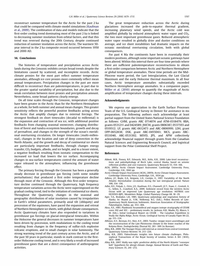
G.H. Miller et al. / Quaternary Science Reviews 29 (2010) 1679e1715 1707
reconstruct summer temperature for the Arctic for the past 2 kathat could be compared with climate-model simulations (Kaufmanet al., 2009). The combination of data and models indicate that thefirst-order cooling trend dominating most of the past 2 ka is linkedto decreasing summer insolation from orbital factors, and that thistrend was reversed during the 20th Century, despite continuedreduction of summer insolation across the Arctic. The warmest 50-year interval in the 2 ka composite record occurred between 1950and 2000 AD.
14. Conclusions
The histories of temperature and precipitation across Arcticlands during the Cenozoic exhibits certain broad trends despite thelimitations caused by scattered, and incomplete records. Arcticclimate proxies for the most part reflect summer temperatureanomalies, although ice core proxies more commonly reflect meanannual temperatures. Precipitation changes in the past are moredifficult to reconstruct than are paleotemperatures, in part due tothe greater spatial variability of precipitation, but also due to theweak correlation between most proxies and precipitation amount.Nevertheless, some broad patterns clearly emerge.
On all time scales through the Cenozoic, temperature changeshave been greater in the Arctic than for the Northern Hemisphereas awhole, for both summer and annualmean changes. This greatersensitivity reflects the powerful positive feedbacks acting acrossthe Arctic that amplify changes due to external forcings. Thestrongest feedback on short timescales (decadal to millennial) isthe expansion and contraction of sea ice, with additional positivefeedbacks from changing seasonal snowcover, changing distribu-tion of forest and tundra ecosystem boundaries, growth and decayof permafrost, and changes in the strength of the ocean’s meridi-onal overturning circulation. On longer timescales (multi-millen-nial), changes in the location and rate of deep convection in theNorth Atlantic, and the growth and decay of continental ice sheetsare particularly important feedbacks, through changes energytransfer, CO2 budgets, albedo, and ice height, and to a lesser extent,a negative feedback resulting from isostatic compensation to theincreased ice load that lowers the ice surface. Accompanyingchanges in sea-surface temperatures control the amount of watervapor released to the atmosphere, influencing the greenhouseeffect.
The primary forcing through the Cenozoic has been a generallysteady decrease in greenhouse gas forcing (with some notableperturbations) that produced a first order temperature declinethrough most of the Cenozoic. Although this first-order tempera-ture decline continued through the Quaternary, high frequencytemperature variations across the Arctic were superimposed on thegradual cooling trend, tied to the initiation of continental ice sheets.Throughout the Quaternary, changes in the seasonal andgeographic distribution of solar insolation caused by irregularitiesin Earth’s orbital parameters, primarily axial tilt (obliquity) andprecession of the equinoxes, have paced the expansion and retreatof Northern Hemisphere ice sheets, with global climate consequences.Arctic Quaternary climates have also responded to variations ingreenhouse gas forcings on glacial-interglacial timescales. Withinthe Holocene the general decreases in summer temperatures havebeen driven by precession, with modulations to the cooling trendresulting from changes in the frequency of sulfur-rich explosivevolcanic eruptions, and to small changes in solar luminosity. Thestrong warming trend of the past century across the Arctic, and ofthe past 50 years in particular, stands in stark contrast to the first-order Holocene cooling trend, and is very likely a result of increasedgreenhouse gases that are a direct consequence of anthropogenicactivities.
The great temperature reduction across the Arctic duringglaciations increased the pole-to-equator thermal gradient,increasing planetary wind speeds, and the Arctic cold wasamplified globally by reduced atmospheric water vapor and CO2,the two most important greenhouse gases. Reduced atmosphericwater vapor resulted in globally drier and dustier conditions onaverage, and ice sheet instabilities had dramatic impacts on theoceanic meridional overturning circulation, both with globalconsequences.
For past 4 Ma the continents have been in essentially theirmodern positions, although some important oceanic gateways havebeen altered.Within this interval there are four time periods wherethere are sufficient paleotemperature reconstructions to obtaina first-order comparison between Arctic and Northern Hemisphereor global temperature anomalies. These time periods are the Mid-Pliocene warm period, the Last Interglaciation, the Last GlacialMaximum and the early Holocene thermal maximum. In all fourcases, Arctic temperature anomalies substantially exceededNorthern Hemisphere average anomalies. In a companion paper,Miller et al. (2010) attempt to quantify the magnitude of Arcticamplification of temperature changes during these intervals.
Acknowledgments
We express our appreciation to the Earth Surface ProcessesTeam of the U.S. Geological Survey in Denver for assistance in mspreparation. The following authors each acknowledge at leastpartial support from the United States National Science Foundationas follows: GHM, grants ARC 0714074 and ATM-0318479; RBA,grants 0531211 and 0424589; JWCW, grants 0806387, 0537593 and0519512; LP, grants ARC-0612473 and ARC-0806999; LDH, grantOPP-0652838; DSK, grant ARC-0455043; MCS, grants ARC-0531040, ARC-0531302. MSVD, JPS, and APW collectivelyacknowledge financial support through grants from the CanadianNatural Sciences and Engineering Research Council, and logisticalsupport from the Polar Continental Shelf Project.
References
Abbott, M.B., Finney, B.P., Edwards, M.E., Kelts, K.R., 2000. Lake-level reconstruc-tions and paleohydrology of Birch Lake, central Alaska, based on seismicreflection profiles and core transects. Quaternary Research 53, 154e166.
ACIA, 2005a. Arctic Climate Impact Assessment. Cambridge University Press,Cambridge, U.K., 1042 pp.
Arctic Climate Impact Assessment (ACIA), 2005b. Arctic Climate Impact Assessment.Cambridge University Press, Cambridge, U.K., 1024 pp.
Adkins, J.F., Boyle, E.A., Keigwin, L.D., Cortijio, E., 1997. Variability of the NorthAtlantic thermohaline circulation during the last interglacial period. Nature390, 154e156.
Adler, R.E., Polyak, L., Ortiz, J.D., Kaufman, D.S., Channell, J.E.T., Xuan, C., Grottoli, A.G., Sellen, E., Crawford, K.A., 2009. Sediment record from the western ArcticOcean with an improved Late Quaternary age resolution: HOTRAX coreHLY0503-8JPC, Mendeleev Ridge. Global Planetary Change 68, 18e29.
Ager, T.A., Brubaker, L.B., 1985. Quaternary palynology and vegetation history ofAlaska. In: Bryant Jr., V.M., Holloway, R.G. (Eds.), Pollen Records of Late-Quaternary North American Sediments. American Association of StratigraphicPalynologists, Dallas, pp. 353e384.
Aksu, A.E., 1985. Planktonic foraminiferal and oxygen isotope stratigraphy of CESARcores 102 and 103 e preliminary results. In: Jackson, H.R., Mudie, P.J., Blasco, S.M. (Eds.), Initial Geological Report on CESAR e The Canadian Expedition toStudy the Alpha Ridge, Arctic Ocean. Geological Survey of Canada Paper 84-22,pp. 115e124.
Alfimov, A.V., Berman, D.I., Sher, A.V., 2003. Tundraesteppe insect assemblages andthe reconstruction of the Late Pleistocene climate in the lower reaches of theKolyma River. Zoologicheskiy Zhurnal 82, 281e300 (in Russian).
Alley, R.B., 2000. The Younger Dryas cold interval as viewed from central Greenland.Quaternary Science Reviews 19, 213e226.
Alley, R.B., 2003. Paleoclimatic insights into future climate challenges. Philo-sophical Transactions of the Royal Society of London, Series A 361 (1810),1831e1849.
Alley, R.B., 2007. Wally was right: predictive ability of the North Atlantic “conveyorbelt” hypothesis for abrupt climate change. Annual Review of Earth and Plan-etary Sciences 35, 241e272.

G.H. Miller et al. / Quaternary Science Reviews 29 (2010) 1679e17151708
Alley, R.B., Ágústsdóttir, A.M., 2005. The 8 k event: cause and consequences ofa major Holocene abrupt climate change. Quaternary Science Reviews 24,1123e1149.
Alley, R.B., Anandakrishnan, S., 1995. Variations in melt-layer frequency in the GISP2ice core: implications for Holocene summer temperatures in central Greenland.Annals of Glaciology 21, 64e70.
Alley, R.B., Cuffey, K.M., 2001. Oxygen- and hydrogen-isotopic ratios of water inprecipitation: beyond paleothermometry. In: Valley, J.W., Cole, D. (Eds.), StableIsotope Geochemistry. Mineralogical Society of America Reviews in Mineralogyand Geochemistry 43, 527e553.
Alley, R.B., Meese, D.A., Shuman, C.A., Gow, A.J., Taylor, K.C., Grootes, P.M., White, J.W.C., Ram, M., Waddington, E.D., Mayewski, P.A., Zielinski, G.A., 1993. Abruptincrease in snow accumulation at the end of the Younger Dryas event. Nature362, 527e529.
Alley, R.B., Shuman, C.A., Meese, D.A., Gow, A.J., Taylor, K.C., Cuffey, K.M.,Fitzpatrick, J.J., Grootes, P.M., Zielinski, G.A., Ram, M., Spinelli, G., Elder, B., 1997.Visual-stratigraphic dating of the GISP2 ice core e basis, reproducibility, andapplication. Journal of Geophysical Research 102, 26,367e26,381.
Alley, R.B., Brook, E.J., Anandakrishnan, S., 2002. A northern lead in the orbital band:northesouth phasing of ice-age events. Quaternary Science Reviews 21 (1e3),431e441.
Alley, R.B., Andrews, J.T., Brigham-Grette, J., Clarke, G.K.C., Cuffey, K.M., Fitzpatrick, J.J., Funder, S., Marshall, S.J., Miller, G.H., Mitrovica, J.X., Muhs, D.R., Otto-Bleisner, B., Polyak, L., White, J.W.C., 2010. History of the Greenland Ice Sheet:Paleoclimatic Insights. Quaternary Science Reviews 29, 1728e1756.
Ammann, C.M., Joos, F., Schimel, D.S., Otto-Bliesner, B.L., Tomas, R.A., 2007. Solarinfluence on climate during the past millennium e results from transientsimulations with the NCAR Climate System Model. Proceedings of the NationalAcademy of Sciences 104 (10), 3713e3718.
Anderson, N.J., Leng, M.J., 2004. Increased aridity during the early Holocene in WestGreenland inferred from stable isotopes in laminated-lake sediments. Quater-nary Science Reviews 23, 841e849.
Anderson, P.M., Lozhkin, A.V., 2001. The stage 3 interstadial complex (Karginskii/middle Wisconsinan interval) of Beringia: variations in paleoenvironments andimplications for paleoclimatic interpretations. Quaternary Science Reviews 20,93e125.
Anderson, P.M., Bartlein, P.J., Brubaker, L.B., Gajewski, K., Ritchie, J.C., 1989. Modernanalogues of late Quaternary pollen spectra from the western interior of NorthAmerica. Journal of Biogeography 16, 573e596.
Anderson, P.M., Bartlein, P.J., Brubaker, L.B., Gajewski, K., Ritchie, J.C., 1991. Vege-tationepolleneclimate relationships for the arcto-boreal region of NorthAmerica and Greenland. Journal of Biogeography 18, 565e582.
Anderson, L., Abbott, M.B., Finney, B.P., 2001. Holocene climate inferred from oxygenisotope ratios in lake sediments, central Brooks Range, Alaska. QuaternaryResearch 55, 313e321.
Anderson, L., Abbott, M.B., Finney, B.P., Edwards, M.E., 2005. Palaeohydrology of theSouthwest Yukon Territory, Canada, based on multiproxy analyses of lakesediment cores from a depth transect. The Holocene 15, 1172e1183.
Anderson, L., Abbott, M.B., Finney, B.P., Burns, S.J., 2006. Erratum to “Regionalatmospheric circulation change in the North Pacific during the Holoceneinferred from lacustrine carbonate oxygen isotopes, Yukon Territory,Canada [Quaternary Research 64 (2005) 21e35]”. Quaternary Research 65,350e351.
Anderson, L., Abbott, M.B., Finney, B.P., Burns, S.J., 2007. Late Holocene moisturebalance variability in the southwest Yukon Territory, Canada. QuaternaryScience Reviews 26, 130e141.
Anderson, R.K., Miller, G.H., Briner, J.P., Lifton, N.A., DeVogel, S.B., 2008. A millennialperspective on Arctic warming from 14C in quartz and plants emerging frombeneath ice caps. Geophysical Research Letters 35, L01502. doi:10.1029/2007GL032057.
Andreev, A.A., Peteet, D.M., Tarasov, P.E., Romanenko, F.A., Filimonova, L.V.,Sulerzhitsky, L.D., 2001. Late Pleistocene interstadial environment on Fad-deyevskiy Island, East-Siberian Sea, Russia. Arctic, Antarctic, and AlpineResearch 33, 28e35.
Andrews, J.T., Smith, L.M., Preston, R., Cooper, T., Jennings, A.E., 1997. Spatial andtemporal patterns of iceberg rafting (IRD) along the East Greenland margin, ca68 N, over the last 14 cal ka. Journal of Quaternary Science 12, 1e13.
Astakhov, V.I., 1995. The mode of degradation of Pleistocene permafrost in WestSiberia. Quaternary International 28, 119e121.
Axford, Y., Briner, J.P., Cooke, C.A., Francis, D.R., Michelutti, N., Miller, G.H., Smol, J.P.,Thomas, E.K., Wilson, C.R., Wolfe, A.P., 2009. Recent changes in a remote Arcticlake are unique within the past 200,000 years. Proceedings of the NationalAcademy of Science. doi:10.1073/pnas.0907094106.
Backman, J., Moran, K., McInroy, D.B., Mayer, L.A., 2006. Expedition 302 scientists.Proceedings of IODP 302. doi:10.2204/iodp.proc.302.2006 Edinburgh (Inte-grated Ocean Drilling Program Management International, Inc.).
Balco, G., Rovey, C.W., Stone, O.H., 2005a. The First Glacial Maximum in NorthAmerica. Science 307, 222.
Balco, G., Stone, O.H., Jennings, C., 2005b. Dating Plio-Pleistocene glacial sedimentsusing the cosmic-ray-produced radionuclides 10Be and 26Al. American Journalof Science 305, 1e41.
Ballantyne, A.P., Rybczynski, N.L., Baker, P.A., Harington, C.R., White, D., 2006.Pliocene Arctic temperature constraints from the growth rings and isotopiccomposition of fossil larch. Palaeogeography, Palaeoclimatology, Palaeoecology242, 188e200.
Barber, V.A., Finney, B.P., 2000. Lake Quaternary paleoclimatic reconstructions forinterior Alaska based on paleolake-level data and hydrologic models. Journal ofPaleolimnology 24, 29e41.
Barber, D.C., Dyke, A., Hillaire-Marcel, C., Jennings, A.E., Andrews, J.T., Kerwin, M.W.,Bilodeau, G., McNeely, R., Southon, J., Morehead, M.D., Gagnon, J.-M., 1999.Forcing of the cold event of 8200 years ago by catastrophic drainage of Lau-rentide lakes. Nature 400, 344e348.
Bard, E., December 2002. Climate shocks e abrupt changes over millennial timescales. Physics Today, 32e38.
Barnekow, L., Sandgren, P., 2001. Palaeoclimate and tree-line changes during theHolocene based on pollen and plant macrofossil records from six lakes atdifferent altitudes in northern Sweden. Review of Palaeobotany and Palynology117, 109e118.
Barron, E.J., Fawcett, P.J., Pollard, D., Thompson, S., 1993. Model simulations ofCretaceous climates e the role of geography and carbon-dioxide. PhilosophicalTransactions of the Royal Society of London Series B-Biological Sciences 341(1297), 307e315.
Bauch, D., Schlosser, P., Fairbanks, R.G., 1995. Freshwater balance and the sources ofdeep and bottom waters in the Arctic Ocean inferred from the distribution ofH218O. Progress in Oceanography 35, 53e80.
Bauch, D., Carstens, J., Wefer, G., 1997. Oxygen isotope composition of living Neo-globoquadrina pachyderma (sin.) in the Arctic Ocean. Earth and PlanetaryScience Letters 146, 47e58.
Bauch, H.A., Erlenkeuser, H., 2003. Interpreting glacial-1nterglacial changes in icevolume and climate from subarctic deep-water foraminiferal d18O. In:Droxler, A.W., Poore, R.Z., Burckle, L.H. (Eds.), Earth’s Climate and OrbitalEccentricity: The Marine Isotope Stage 11 Question. American GeophysicalUnion Geophysical Monograph Series 137, 87e102.
Bauch, H.A., Kandiano, E.S., 2007. Evidence for early warming and cooling in NorthAtlantic surface waters during the last interglacial. Paleoceanography 22,PA1201. doi:10.1029/2005PA001252.
Bauch, H.A., Erlenkeuser, H., Fahl, K., Spielhagen, R.F., Weinelt, M.S., Andruleit, H.,Henrich, R., 1999. Evidence for a steeper Eemian than Holocene sea surfacetemperature gradient between Arctic and sub-Arctic regions. Palaeogeography,Palaeoclimatology, Palaeoecology 145, 95e117.
Bauch, H.A., Erlenkeuser, H., Helmke, J.P., Struck, U., 2000. A paleoclimatic evalua-tion of marine oxygen isotope stage 11 in the high-northern Atlantic (Nordicseas). Global and Planetary Change 24, 27e39.
Behl, R.J., Kennett, J.P., 1996. Brief interstadial events in the Santa Barbara Basin, NEPacific, during the past 60 kyr. Nature 379, 243e246.
Bendle, J.A., Rosell-Melé, A., 2004. Distributions of Uk37 and Uk
37 in the surfacewaters and sediments of the Nordic Seas: implications for paleoceanography.Geochemistry, Geophysics, Geosystems 5, 3589e3600. doi:10.1029/2004GC000741. Q11013.
Bennike, O., Brodersen, K.P., Jeppesen, E., Walker, I.R., 2004. Aquatic invertebratesand high latitude paleolimnology. In: Pienitz, R., Douglas, M.S.V., Smol, J.P.(Eds.), Long-Term Environmental Change in Arctic and Antarctic Lakes. Springer,Dordrecht, pp. 159e186.
Berger, A., Loutre, M.F., 1991. Insolation values for the climate of the last 10 millionyears. Quaternary Science Reviews 10, 297e317.
Berger, A., Loutre, M.F., Laskar, J., 1992. Stability of the astronomical frequenciesover the Earth’s history for paleoclimate studies. Science 255 (5044),560e566.
Berner, R.A., Kothavala, Z., 2001. GEOCARB III: a revised model of atmospheric CO2over Phanerozoic time. American Journal of Science 301 (2), 182e204.
Bice, K.L., Birgel, D., Meyers, P.A., Dahl, K.A., Hinrichs, K.U., Norris, R.D., 2006.A multiple proxy and model study of Cretaceous upper ocean temperatures andatmospheric CO2 concentrations. Paleoceanography 21 (2), PA2002.
Bigelow, N., Brubaker, L.B., Edwards, M.E., Harrison, S.P., Prentice, I.C., Anderson, P.M., Andreev, A.A., Bartlein, P.J., Christensen, T.R., Cramer, W., Kaplan, J.O.,Lozhkin, A.V., Matveyeva, N.V., Murrary, D.F., McGuire, A.D., Razzhivin, V.Y.,Ritchie, J.C., Smith, B., Walker, D.A., Gajewski, K., Wolf, V., Holmqvist, B.H.,Igarashi, Y., Kremenetskii, K., Paus, A., Pisaric, M.F.J., Volkova, V.S., 2003. Climatechange and Arctic ecosystems e 1. Vegetation changes north of 55�N betweenthe last glacial maximum, mid-Holocene, and present. Journal of GeophysicalResearch 108 (D19), 8170. doi:10.1029/2002JD002558.
Billups, K., Channell, J.E.T., Zachos, J., 2002. Late Oligocene to early Miocenegeochronology and paleoceanography from the subantarctic South Atlantic.Paleoceanography 17 (1), 1004. doi:10.1029/2000PA000568.
Binney, H.A., Willis, K.J., Edwards, M.E., Bhagwat, S.A., Anderson, P., Andreev, A.A.,Blaauw, M., Damblon, F., Haesaerts, P., Kienast, F., Kremenetski, K.V.,Krivonogov, S.K., Lozhkin, A.V., Macdonald, G.M., Novenko, E.Y., Oksanen, P.,Sapelko, T.V., Valiranta, M., Vazhenina, L., 2009. The distribution of LateQuaternary woody taxa in Eurasia: evidence from a new macrofossil database.Quaternary Science Reviews 28, 2445e2464.
Birks, H.H., 1991. Holocene vegetational history and climatic change in westSpitzbergen e plant macrofossils from Skardtjorna, an arctic lake. The Holocene1, 209e218.
Birks, H.J.B., 1998. Numerical tools in palaeolimnology e progress, potentialities,and problems. Journal of Paleolimnology 20, 307e332.
Boellstorff, J., 1978. North American Pleistocene stages reconsidered in light ofprobably PlioceneePleistocene continental glaciation. Science 202 (2004365),305e307.
Bohaty, S.M., Zachos, J.C., 2003. Significant Southern Ocean warming event in thelate middle Eocene. Geology 31, 1017e1020. doi:10.1130/G19800.1.

G.H. Miller et al. / Quaternary Science Reviews 29 (2010) 1679e1715 1709
Box, J.E., Bromwich, D.H., Veenhuis, B.A., Bai, L.-S., Stroeve, J.C., Rogers, J.C.,Steffen, K., Haran, T., Wang, S.-H., 2006. Greenland ice-sheet surface massbalance variability (1988e2004) from calibrated Polar MM5 output. Journal ofClimate 19 (12), 2783e2800.
Braconnot, P., Otto-Bliesner, B., Harrison, S., Joussaume, F.S., Peterchmitt, J.-Y., Abe-Ouchi, A., Crucifix, M., Driesschaert, E., Fichefet, T., Hewitt, C.D., Kageyama, M.,Kitoh, A., Laine, A., Loutre, M.-F., Marti, O., Merkel, U., Ramstein, G., Valdes, P.,Weber, S.L., Yu, Y., Zhao, Y., 2007. Results of PMIP2 coupled simulations of theMid-Holocene and Last Glacial Maximum e part 1: experiments and large-scalefeatures. Climates of the Past 3, 261e277.
Bradley, R.S., 1999. Paleoclimatology: Reconstructing Climates of the Quaternary,second ed. Academic Press, New York, 613 pp.
Bradley, R.S., 2000. Past global changes and their significance for the future.Quaternary Science Reviews 19, 391e402.
Bradley, R.S., England, J.H., 2008. The Younger Dryas and the Sea of Ancient Ice.Quaternary Research 70, 1e10.
Bradley, R.S., Jones, P.D. (Eds.), 1992. Climate Since AD 1500. Routlege, London, 677pp.
Bradley, R.S., Briffa, K.R., Cole, J., Osborn, T.J., 2003a. The climate of the lastmillennium. In: Alverson, K.D., Bradley, R.S., Pedersen, T.F. (Eds.), Paleoclimate,Global Change and the Future. Springer, Berlin, pp. 105e141.
Bradley, R.S., Hughes, M.K., Diaz, H.F., 2003b. Climate in Medieval time. Science 302,404e405. doi:10.1126/science.1090372.
Brassell, S.C., Eglinton, G., Marlowe, I.T., Pflaumann, U., Sarnthein, M., 1986.Molecular stratigraphy e a new tool for climatic assessment. Nature 320,129e133.
Bray, P.J., Blockey, S.P.E., Coope, G.R., Dadswell, L.F., Elias, S.A., Lowe, J.J., Pollard, A.M.,2006. Refining mutual climatic range (MCR) quantitative estimates of paleo-temperature using ubiquity analysis. Quaternary Science Reviews 25 (15e16),1865e1876.
Briffa, K., Cook, E., 1990. Methods of response function analysis. In: Cook, E.R.,Kairiukstis, L.A. (Eds.), Methods of Dendrochronology. Kluwer, Dordrecht, TheNetherlands, pp. 165e178.
Briffa, K.R., Osborn, T.J., Schweingruber, F.H., Harris, I.C., Jones, P.D., Shiyatov, S.G., Vaganov, E.A., 2001. Low-frequency temperature variations froma northern tree ring density network. Journal of Geophysical Research 106,2929e2941.
Brigham, J.K., 1985. Marine stratigraphy and amino acid geochronology of theGubik Formation, western Arctic Coastal Plain, Alaska. Doctoral dissertation,University of Colorado, Boulder. U.S. Geological Survey Open-File Report 85-381, 21 pp.
Brigham-Grette, J., Carter, L.D., 1992. Pliocene marine transgressions of northernAlaska e circumarctic correlations and paleoclimate. Arctic 43 (4), 74e89.
Brigham-Grette, J., Hopkins, D.M., 1995. Emergent-marine record and paleoclimateof the last interglaciation along the northwest Alaskan coast. QuaternaryResearch 43, 154e173.
Brigham-Grette, J., Lozhkin, A.V., Anderson, P.M., Glushkova, O.Y., 2004. Paleo-environmental conditions in western Beringia before and during the LastGlacial Maximum. In: Madsen, D.B. (Ed.), Entering America: Northeast Asia andBeringia Before the Last Glacial Maximum. University of Utah Press, pp. 29e61(Chapter 2).
Brinkhuis, H., Schouten, S., Collinson, M.E., Sluijs, A., Damsfte, J.S.S., Dickens, G.R.,Huber, M., Cronin, T.M., Onodera, J., Takahashi, K., Bujak, J.P., Stein, R., van derBurgh, J., Eldrett, J.S., Harding, I.C., Lotter, A.F., Sangiorgi, F., Cittert, H.V.V., deLeeuw, J.W., Matthiessen, J., Backman, J., Moran, K., Expedition 302 Scientists,2006. Episodic fresh surface waters in the Eocene Arctic Ocean. Nature 441(7093), 606e609.
Broecker, W.S., 2001. Was the Medieval warm period global? Science 291 (5508),1497e1499. doi:10.1126/science.291.5508.1497.
Broecker, W.S., Hemming, S., 2001. Climate swings come into focus. Nature 294(5550), 2308e2309.
Brouwers, E.M., 1987. On Prerygocythereis vunnieuwenhuisei Brouwers sp.nov. In:Bate, R.H., Home, D.J., Neale, J.W., Siveter, D.J. (Eds.), A Stereo-atlas of Ostra-code Shells Part 1. British Micropaleontological Society, London, vol. 14, pp.17e20.
Burns, S.J., Fleitmann, D., Matter, D., Kramers, J., Al-Subbary, A.A., 2003. IndianOcean climate and an absolute chronology over Dansgaard/Oeschger Events 9to 13. Science 301, 1365e1377.
Calkin, P.E., 1988. Holocene glaciation of Alaska (and adjoining Yukon Territory,Canada). Quaternary Science Reviews 7, 159e184.
CircumArctic PaleoEnvironments (CAPE) e Last Interglacial Project Members(Anderson, P., Bennike, O., Bigelow, N., Brigham-Grette, J., Duvall, M., Edwards,M., Frechette, B., Funder, S., Johnsen, S., Knies, J., Koerner, R., Lozhkin, A.,Marshall, S., Matthiessen, J., Macdonald, G., Miller, G., Montoya, M., Muhs, D.,Otto-Bliesner, B., Overpeck, J., Reeh, N., Sejrup, H.P., Spielhagen, R., Turner C.,Velichko, A., 2006. Last Interglacial Arctic warmth confirms polar amplificationof climate change. Quaternary Science Reviews 25, 1383e1400.
Carter, L.D., Brigham-Grette, J., Marincovich Jr., L., Pease, V.L., Hillhouse, U.S., 1986.Late Cenozoic Arctic Ocean sea ice and terrestrial paleoclimate. Geology 14,675e678.
Chapin III, F.S., Sturm, M., Serreze, M.C., Mcfadden, J.P., Key, J.R., Lloyd, A.H., Rupp, T.S., Lynch, A.H., Schimel, J.P., Beringer, J., Chapman, W.L., Epstein, H.E.,Euskirchen, E.S., Hinzman, L.D., Jia, G., Ping, C.L., Tape, K.D., Thompson, C.D.C.,Walker, D.A., Welker, J.M., 2005. Role of land-surface changes in Arctic summerwarming. Science 310, 657e660.
Chapman, M.R., Shackleton, N.J., Duplessy, J.-C., 2000. Sea surface temperaturevariability during the last glacial-interglacial cycle eAssessing the magnitudeand pattern of climate change in the North Atlantic. Palaeogeography, Palae-oclimatology, Palaeoecology 157, 1e25.
Clark, P.U., Pollard, D., 1998. Origin of the Middle Pleistocene transition by ice sheeterosion of regolith. Paleoceanography 13, 1e9.
Clark, P.U., McCabe, A.M., Mix, A.C., Weaver, A.J., 2004. Rapid rise of sea level 19,000years ago and its global implications. Science 304, 1141e1144.
Clark, P.U., Archer, D., Pollard, D., Blum, J.D., Rial, J.A., Brovkin, V., Mix, A.C., Pisias, N.G., Roy, M., 2006. The middle Pleistocene transition: characteristics, mecha-nisms, and implications for long-term changes in atmospheric pCO2. Quater-nary Science Reviews 25, 3150e3184.
Clayden, S.L., Cwynar, L.C., MacDonald, G.M., Velichko, A.A., 1997. Holocene pollenand stomates from a forest-tundra site on the Taimyr Peninsula, Siberia. Arcticand Alpine Research 29, 327e333.
Climate Long-Range Investigation Mapping and Prediction (CLIMAP) ProjectMembers, 1981. Seasonal reconstructions of the Earth’s surface at the last glacialmaximum. In: Map and Chart Series MC-36. Geological Society of America.1e18.
Climate Long-Range Investigation Mapping and Prediction (CLIMAP) ProjectMembers, 1984. The last interglacial ocean. Quaternary Research 21, 123e224.
Cockford, S.J., Frederick, S.G., 2007. Sea ice expansion in the Bering Sea during theNeoglacial e evidence from archeozoology. The Holocene 17, 699e706.
Cohen, A.S., 2003. Paleolimnology e the History and Evolution of Lake Systems.Oxford University Press, Oxford, U.K., 528 pp.
Colinvaux, P.A., 1964. The environment of the Bering Land Bridge. EcologicalMonographs 34, 297e329.
Conte, M.H., Sicre, M., Rühlemann, C., Weber, J.C., Schulte, S., Schulz-Bull, D.,Blanz, T., 2006. Global temperature calibration of the alkenone unsaturationindex (U370K ) in surface waters and comparison with surface sediments.Geochemistry, Geophysics, Geosystems 7, Q02005. doi:10.1029/2005GC001054.
Cronin, T.M., Dwyer, G.S., Kamiyac, T., Schwedea, S., Willarda, D.A., 2003. MedievalWarm Period, Little Ice Age and 20th century temperature variability fromChesapeake Bay. Global and Planetary Change 36, 17e29.
Crowley, T.J., 1998. Significance of tectonic boundary conditions for paleoclimatesimulations. In: Crowley, T.J., Burke, K.C. (Eds.), Tectonic Boundary Conditionsfor Climate Reconstructions. Oxford University Press, New York, pp. 3e17.
Crowley, T.J., 2000. Causes of climate change over the past 1000 years. Science 289,270e277.
Crowley, T.J., Lowery, T., 2000. How warm was the Medieval warm period? Ambio29, 51e54.
Crowley, T.J., Baum, S.K., Kim, K.Y., Hegerl, G.C., Hyde, W.T., 2003. Modeling oceanheat content changes during the last millennium. Geophysical Research Letters30, 1932. doi:10.1029/2003GL017801.
Cuffey, K.M., Clow, G.D., 1997. Temperature, accumulation, and ice sheet elevation incentral Greenland through the last deglacial transition. Journal of GeophysicalResearch 102 (C12), 26,383e26,396.
Cuffey, K.M., Clow, G.D., Alley, R.B., Stuiver, M., Waddington, E.D., Saltus, R.W., 1995.Large arctic temperature change at the WisconsineHolocene glacial transition.Science 270 (5235), 455e458.
D’Arrigo, R., Wilson, R., Jacoby, G., 2006. On the long-term context for late twentiethcentury warming. Journal of Geophysical Research 111, D03103. doi:10.1029/2005JD006352.
Dahe, Q., Petit, J.R., Jouzel, J., Stievenard, M., 1994. Distribution of stable isotopes insurface snow along the route of the 1990 International Trans-Antarctic Expe-dition. Journal of Glaciology 40, 107e118.
Dahl, S.O., Nesje, A., 1996. A new approach to calculating Holocene winter precip-itation by combining glacier equilibrium-line altitudes and pine-tree limits:a case study from Hardangerjokulen, central southern Norway. The Holocene 6(4), 381e398. doi:10.1177/095968369600600401.
Dahl-Jensen, D., Mosegaard, K., Gundestrup, N., Clow, G.D., Johnsen, S.J., Hansen, A.W., Balling, N., 1998. Past temperatures directly from the Greenland Ice Sheet.Science 282, 268e271.
Dansgaard, W., 1964. Stable isotopes in precipitation. Tellus 16, 436e468.Dansgaard, W., White, J.W.C., Johnsen, S.J., 1989. The abrupt termination of the
Younger Dryas climate event. Nature 339, 532e534.Darby, D.A., Polyak, L., Bauch, H., 2006. Past glacial and interglacial conditions in the
Arctic Ocean and marginal seas e a review. In: Wassman, P. (Ed.), Structure andFunction of Contemporary Food Webs on Arctic Shelves e a Pan-ArcticComparison. Progress in Oceanography 71, 129e144.
Delworth, T.L., Knutson, T.R., 2000. Simulation of early 20th century global warm-ing. Science 287, 2246.
de Vernal, A., Hillaire-Marcel, C., Darby, D.A., 2005. Variability of sea ice cover in theChukchi Sea (western Arctic Ocean) during the Holocene. Paleoceanography 20,PA4018. doi:10.1029/2005PA001157.
Denton, G.H., Alley, R.B., Comer, G.C., Broecker, W.S., 2005. The role of seasonality inabrupt climate change. Quaternary Science Reviews 24, 1159e1182.
Digerfeldt, G., 1988. Reconstruction and regional correlation of Holocene lake-levelfluctuations in Lake Bysjön, South Sweden. Boreas 17, 237e263.
Donnadieu, Y., Pierrehumbert, R., Jacob, R., Fluteau, F., 2006. Modelling the primarycontrol of paleogeography on Cretaceous climate. Earth and Planetary ScienceLetters 248, 426e437.
Douglas, M.S.V., 2007. Environmental change at high latitudes. In: Starratt, S.W.(Ed.), Geological and Environmental Applications of the Diatom e Pond Scum toCarbon Sink. The Paleontological Society Papers, vol. 13, pp. 169e179.

G.H. Miller et al. / Quaternary Science Reviews 29 (2010) 1679e17151710
Douglas, M.S.V., Smol, J.P., Blake Jr., W., 1994. Marked post-18th century environ-mental change in high Arctic ecosystems. Science 266, 416e419.
Douglas, M.S.V., Smol, J.P., Pienitz, R., Hamilton, P., 2004. Algal indicators of envi-ronmental change in arctic and antarctic lakes and ponds. In: Pienitz, R.,Douglas, M.S.V., Smol, J.P. (Eds.), Long-Term Environmental Change in Arctic andAntarctic Lakes. Springer, Dordrecht, pp. 117e157.
Dowsett, H.J., Chandler, M.A., Robinson, M.M., 2009. Surface temperatures of theMid-Pliocene North Atlantic Ocean: implications for future climate. Philo-sophical Transactions of the Royal Society of London A 367, 69e84.
Droxler, A.W., Farrell, J.W., 2000. Marine isotope stage 11 (MIS11): new insights fora warm future. Global and Planetary Change 24 (1), 1e5.
Droxler, A.W., Alley, R.B., Howard, W.R., Poore, R.Z., Burckle, L.H., 2003. Unique andexceptionally long interglacial marine isotope stage 11 e window into Earthfuture climate. In: Droxler, A.W., Poore, R.Z., Burckle, L.H. (Eds.), Earth’s Climateand Orbital Eccentricity e The Marine Isotope Stage 11 Question. GeophysicalMonograph 137. American Geophysical Union, pp. 1e14.
Duk-Rodkin, A., Barendregt, R.W., Froese, D.G., Weber, F., Enkin, R.J., Smith, I.R.,Zazula, G.D., Waters, P., Klassen, R., 2004. Timing and Extent of Plio-Pleistoceneglaciations in North-Western Canada and East-Central Alaska. In: Ehlers, J.,Gibbard, P.L. (Eds.), Quaternary Glaciations-Extent and Chronology, Part II,North America. Elsevier, New York, pp. 313e345.
Dyke, A.S., Savelle, J.M., 2001. Holocene history of the Bering Sea bowheadwhale (Balaena mysticetus) in its Beaufort Sea summer grounds offsouthwestern Victoria Island, western Canadian Arctic. QuaternaryResearch 55, 371e379.
Dyke, A.S., Moore, A., Robertson, L., 2003. Deglaciation of North America. GeologicalSurvey of Canada. Open File 1574. (published on CD-ROM).
Dykoski, C.A., Edwards, R.L., Cheng, H., Yuan, D., Cai, Y., Zhang, M., Lin, Y., Qing, J.,An, Z., Revenaugh, J., 2005. A high-resolution, absolute-dated Holocene anddeglacial Asian monsoon record from Dongge Cave, China. Earth and PlanetaryScience Letters 233, 71e86.
Edwards, M.E., Bigelow, N.H., Finney, B.P., Eisner, W.R., 2000. Records of aquaticpollen and sediment properties as indicators of late-Quaternary Alaskan lakelevels. Journal of Paleolimnology 24, 55e68.
Eldrett, J.S., Harding, I.C., Wilson, P.A., Butler, E., Roberts, A.P., 2007. Continental icein Greenland during the Eocene and Oligocene. Nature 446, 176e179.
Elias, S.A., 2007. Beetle records e Late Pleistocene North America. In: Elias, S.A.(Ed.), Encyclopedia of Quaternary Science. Elsevier, Amsterdam, pp.222e236.
Elias, S.A., Anderson, K., Andrews, J.T., 1996. Late Wisconsin climate in the north-eastern United States and southeastern Canada, reconstructed from fossil beetleassemblages. Journal of Quaternary Science 11, 417e421.
Elias, S.A., Andrews, J.T., Anderson, K.H., 1999. New insights on the climaticconstraints on the beetle fauna of coastal Alaska derived from the mutualclimatic range method of paleoclimate reconstruction. Arctic, Antarctic, andAlpine Research 31, 94e98.
Elias, S.A., Matthews Jr., J.V., 2002. Arctic North American seasonal temperatures inthe Pliocene and Early Pleistocene, based on mutual climatic range analysis offossil beetle assemblages. Canadian Journal of Earth Sciences 39, 911e920.
Ellis, J.M., Calkin, P.E., 1984. Chronology of Holocene glaciation, central BrooksRange, Alaska. Geological Society of America Bulletin 95, 897e912.
England, J.H., Furze, M.F.A., 2008. New evidence from the western Canadian ArcticArchipelago for the resubmergence of Bering Strait. Quaternary Research 70,60e67.
England, J.H., Lakeman, T.R., Lemmen, D.S., Bednarski, J.M., Stewart, T.G., Evans, D.J.A., 2008. A millennial-scale record of Arctic Ocean sea ice variability and thedemise of the Ellesmere Island ice shelves. Geophysical Research Letters 35,L19502. doi:10.1029/2008GL034470.
EPICA Community Members, 2004. Eight glacial cycles from an Antarctic ice core.Nature 429, 623e628.
Epstein, S., Buchsbaum, H., Lowenstam, H., Urey, H.C., 1953. Revised carbonate-water isotopic temperature scale. Geological Society of America Bulletin 64,1315e1325.
Erez, J., Luz, B., 1982. Temperature control of oxygen-isotope fractionation ofcultured planktonic foraminifera. Nature 297, 220e222.
Esper, J., Cook, E.R., Schweingruber, F.H., 2002. Low-frequency signals in long tree-ring chronologies for reconstructing past temperature variability. Science 295,2250e2253.
Esper, J., Schweingruber, F.H., 2004. Large-scale treeline changes recorded in Siberia.Geophysical Research Letters 31, L06202. doi:10.1029/2003GL019178.
Fairbanks, R.G., 1989. A 17,000-year glacio-eustatic sea level record e influence ofglacial melting rates on the Younger Dryas event and deep-ocean circulation.Nature 343, 612e616.
Farrera, I., Harrison, S.P., Prentice, I.C., Ramstein, G., Guiot, J., Bartlein, P.J.,Bonnelle, R., Bush, M., Cramer, W., von Grafenstein, U., Holmgren, K.,Hooghiemstra, H., Hope, G., Jolly, D., Lauritzen, S.-E., Ono, Y., Pinot, S., Stute, M.,Yu, G., 1999. Tropical climates at the Last Glacial Maximum: a new synthesis ofterrestrial palaeoclimate data. I. Vegetation, lake-levels and geochemistry.Climate Dynamics 15, 823e856.
Fisher, D.A., 1979. Comparison of 100,000 years of oxygen isotope and insolubleimpurity profiles from the Devon Island and Camp Century ice cores. Quater-nary Research 11, 299e304.
Fisher, D.A., Koerner, R.M., 2003. Holocene ice core climate history, a multi-variableapproach. In: Mackay, A., Battarbee, R., Birks, J., Oldfield, F. (Eds.), Global Changein the Holocene. Arnold, London, pp. 281e293.
Fisher, D., Koerner, R.M., Reeh, N., 1995. Holocene climatic records from Agassiz IceCap, Ellesmere Island, NWT, Canada. The Holocene 5, 19e24.
Fisher, D.A., Koerner, R.M., Bourgeois, J.C., Zielinski, G., Wake, C., Hammer, C.U.,Clausen, H.B., Gundestrup, N., Johnsen, S., Goto-Azuma, K., Hondoh, T., Blake, E.,Gerasimoff, M., 1998. Penny Ice Cap cores, Baffin Island, Canada, and the Wis-consinan Foxe Dome connection e two states of Hudson Bay ice cover. Science279, 692e695.
Fisher, D.A., Wake, C., Kreutz, K., Yalcin, K., Steig, E., Mayewski, P., Anderson, L.,Aheng, J., Rupper, S., Zdanowicz, C., Demuth, M., Waskiewicz, M., Dahl-Jensen, D., Goto-Azuma, K., Bourgeois, J.B., Koerner, R.M., Sekerka, J.,Osterberg, E., Abbott, M.B., Finney, B.P., Burns, S.J., 2004. Stable isotope recordsfrom Mount Logan, eclipse ice cores and nearby Jellybean Lake. Water cycle ofthe North Pacific over 2000 years and over five vertical kilometers e suddenshift and tropical connections. Geographie Physique et Quaternaire 58,9033e9048.
Flowers, G.E., Björnsson, H., Geirsdóttir, Á., Miller, G.H., Black, J.L., Clarke, G.K.C.,2008. Holocene climate conditions and glacier variation in central Iceland fromphysical modelling and empirical evidence. Quaternary Science Reviews 27,797e813.
Francis, J.E., 1988. A 50-million-year-old fossil forest from Strathcona Fiord, Elles-mere Island, Arctic Canada e evidence for a warm polar climate. Arctic 41 (4),314e318.
Fricke, H.C., O’Neil, J.R., 1999. The correlation between 18O/16O ratios of meteoricwater and surface temperature: its use in investigating terrestrial climatechange over geologic time. Earth and Planetary Science Letters 170, 181e196.
Fritts, H.C., 1976. Tree Rings and Climate. London Academic Press, London, U.K., 576pp.
Fronval, T., Jansen, E., 1997. Eemian and early Weichselian (140e60 ka) paleo-ceanography and paleoclimate in the Nordic seas with comparisons to Holo-cene conditions. Paleoceanography 12, 443e462.
Funder, S., 1989. Quaternary geology of East Greenland. In: Fulton, R.J. (Ed.),Quaternary Geology of Canada and Greenland, Geological Society of AmericaDecade of North American Geology K1, pp. 756e763.
Funder, S., Bennike, O., Böcher, J., Israelson, C., Petersen, K.S., Simonarson, L.A., 2001.Late Pliocene Greenland e the Kap København formation in North Greenland.Bulletin of the Geological Society of Denmark 48, 177e184.
Funder, S., Demidov, I., Yelovicheva, Y., 2002. Hydrography and mollusc faunas ofthe Baltic and the White Sea-North Sea seaway in the Eemian. Palaeogeography,Palaeoclimatology, Palaeoecology 184, 275e304.
Fyles, J.G., Marincovich Jr., L., Mathews Jr., J.V., Barendregt, R., 1991. Unique molluscfind in the Beaufort Formation (Pliocene) Meighen Island, Arctic Canada. In:Current Research, Part B. Geological Survey of Canada, pp. 461e468. Paper 91-1B.
Gajewski, K., MacDonald, G.M., 2004. Palynology of North American Arctic Lakes. In:Pienitz, R., Douglas, M.S.V., Smol, J.P. (Eds.), Long Term Environmental Change inArctic and Antarctic Lakes. Springer, Netherlands, pp. 89e116.
Geirsdóttir, A., Miller, G.H., Wattrus, N.J., Björnsson, H., Thors, K., 2008. Stabili-zation of glaciers terminating in closed water bodies: evidence and broaderimplications. Geophysical Research Letters 35, L17502. doi:10.1029/2008GL034432.
Geirsdóttir, A., Miller, G.H., Thordarson, T., Olafsdottir, K., 2009a. A 2000 year recordof climate variations reconstructed from Haukadalsvatn, West Iceland. Journalof Paleolimnology 41, 95e115. doi:10.1007/s10933-008-9253-z.
Geirsdóttir, Á., Miller, G.H., Axford, Y., Ólafsdóttir, S., 2009b. Holocene glacier andclimate history of Iceland. Quaternary Science Reviews 28, 2107e2118.
Gervais, B.R., MacDonald, G.M., Snyder, J.A., Kremenetski, C.V., 2002. Pinus sylvestristreeline development and movement on the Kola Peninsula of Russia e pollenand stomate evidence. Journal of Ecology 90, 627e638.
Gildor, H., Tziperman, E., Toggweiler, J.R., 2002. Sea ice switch mechanism andglacialeinterglacial CO2 variations. Global Biogeochemical Cycles 16.doi:10.1029/2001GB001446.
Goetcheus, V.G., Birks, H.H., 2001. Full-glacial upland tundra vegetation preservedunder tephra in the Beringia National Park, Seward Peninsula, Alaska. Quater-nary Science Reviews 20 (1e3), 135e147.
Goodfriend, G.A., Brigham-Grette, J., Miller, G.H., 1996. Enhanced age resolution ofthe marine quaternary record in the Arctic using aspartic acid racemizationdating of bivalve shells. Quaternary Research 45, 176e187.
Goosse, H., Renssen, H., Timmermann, A., Bradley, R.A., 2005. Internal and forcedclimate variability during the last millennium e a model-data comparisonusing ensemble simulations. Quaternary Science Reviews 24, 1345e1360.
Gradstein, F.M., Ogg, J.G., Smith, A.G. (Eds.), 2004. A Geologic Time Scale. CambridgeUniversity Press, Cambridge, 589 pp.
Grice, K., Klein Breteler, W.C.M., Schoten, S., Grossi, V., de Leeuw, J.W., SinningeDamste, J.S., 1998. Effects of zooplankton herbivory on biomarker proxy records.Paleoceanography 13, 686e693.
Grove, J.M., 1988. The Little Ice Age. Methuen, London, 498 pp.Grootes, P.M., Stuiver, M., White, J.W.C., Johnsen, S., Jouzel, J., 1993. Comparison of
oxygen isotope records from the GISP2 and GRIP Greenland ice cores. Nature366, 552e554. doi:10.1038/366552a0.
Grudd, H., Briffa, K.R., Karlén, W., Bartholin, T.S., Jones, P.D., Kromer, B., 2002.A 7400-year tree-ring chronology in northern Swedish Lapland e naturalclimatic variability expressed on annual to millennial timescales. The Holocene12, 657e666.
Gudina, V.I., Kryukov, V.D., Levchuk, L.K., Sudakov, L.A., 1983. Upper-Pleistocenesediments in north-eastern Taimyr. Bulletin of Commission on QuaternaryResearches 52, 90e97 (in Russian).
G.H. Miller et al. / Quaternary Science Reviews 29 (2010) 1679e1715 1711
Hammarlund, D., Barnekow, L., Birks, H.J.B., Buchardt, B., Edwards, T.W.D., 2002.Holocene changes in atmospheric circulation recorded in the oxygen-isotopestratigraphy of lacustrine carbonates from northern Sweden. The Holocene 12,339e351.
Hammarlund, D., Björck, S., Buchardt, B., Israelson, C., Thomsen, C.T., 2003. Rapidhydrological changes during the Holocene revealed by stable isotope records oflacustrine carbonates from Lake Igelsjön, southern Sweden. Quaternary ScienceReviews 22, 353e370.
Hannon, G.E., Gaillard, M.J., 1997. The plant-macrofossil record of past lake-levelchanges. Journal of Paleolimnology 18, 15e28.
Hantemirov, R.M., Shiyatov, S.G., 2002. A continuous multi-millennial ring-widthchronology in Yamal, northwestern Siberia. The Holocene 12 (6), 717e726.
Helmke, J.P., Bauch, H.A., 2003. Comparison of glacial and interglacial conditionsbetween the polar and subpolar North Atlantic region over the last five climaticcycles. Paleoceanography 18 (2), 1036. doi:10.1029/2002PA000794.
Heinrich, R., Baumann, K.-H., 1994. Evolution of the Norwegian current and theScandinavian ice sheets during the past 2.6 m.y.: evidence from ODP Leg 104biogenic carbonate and terrigenous records. Palaeogeography, Palae-oclimatology, Palaeoecology 108, 75e94.
Herbert, T.D., 2003. Alkenone paleotemperature determinations. In: Elderfield, H.,Turekian, K.K. (Eds.), Treatise in Marine Geochemistry. Elsevier, Amsterdam, pp.391e432.
Hoffmann, G., Werner, M., Heimann, M., 1998. Water isotope module of the ECHAMatmospheric general circulation model e a study on timescales from days toseveral years. Journal of Geophysical Research 103, 16,871e16,896.
Holland, M.H., Bitz, C.M., Tremblay, B., 2006. Future abrupt reductions in thesummer Arctic sea ice. Geophysical Research Letters 33, L23503. doi:10.1029/2006GL028024.
Hu, F.S., Shemesh, A., 2003. A biogenic-silica d18O record of climatic change duringthe last glacialeinterglacial transition in southwestern Alaska. QuaternaryResearch 59, 379e385.
Hu, F.S., Ito, E., Brown, T.A., Curry, B.B., Engstrom, D.R., 2001. Pronounced climaticvariations in Alaska during the last two millennia. Proceedings of the NationalAcademy of Science 98, 10552e10556.
Huang, Y., Shuman, B., Wang, Y., Webb III, T., 2002. Hydrogen isotope ratios ofpalmitic acid in lacustrine sediments record late Quaternary climate variations.Geology 30, 1103e1106.
Huber, C., Leuenberger, M., Spahni, R., Flückiger, J., Schwander, J., Stocker, T.F.,Johnsen, S., Landais, A., Jouzel, J., 2006. Isotope calibrated Greenland tempera-ture record over Marine Isotope Stage 3 and its relation to CH4. Earth andPlanetary Science Letters 243 (3e4), 504e519.
Hughen, K., Overpeck, J., Anderson, R.F., Williams, K.M., 1996. The potential forpalaeoclimate records from varved Arctic lake sediments: Baffin Island, EasternCanadian Arctic. In: Kemp, A.E.S. (Ed.), Lacustrine Environments. Palae-oclimatology and Palaeoceanography from Laminated Sediments. GeologicalSociety of London, Special Publications, vol. 116, pp. 57e71.
Hughes, M.K., Diaz, H.F., 1994. Was there a ‘Medieval Warm Period’ and if so, whereand when? Journal of Climatic Change 265, 109e142.
Huybers, P., 2006. Early Pleistocene glacial cycles and the integrated summerinsolation forcing. Science 313, 508e511.
Hyvärinen, H., 1976. Flandrian pollen deposition rates and tree-line history innorthern Fennoscandia. Boreas 5 (3), 163e175.
Ilyashuk, E.A., Ilyashuk, B.P., Hammarlund, D., Larocque, I., 2005. Holocene climaticand environmental changes inferred from midge records (Diptera: Chirono-midae, Chaoboridae, Ceratopogonidae) at Lake Berkut, southern Kola Peninsula,Russia. Holocene 15, 897e914.
Imbrie, J., Kipp, N.G., 1971. A new micropaleontological method for QuantitativePaleoclimatology: application to a late Pleistocene Caribbean Core. In: Tur-ekian, K.K. (Ed.), The Late Cenozoic Glacial Age. Yale Univeristy Press, NewHaven, CT, pp. 71e181.
Intergovernmental Panel on Climate Change (IPCC), 2007. Summary for policy-makers. Contribution of Working Group I to the Fourth Assessment Report ofthe Intergovernmental Panel on Climate Change. In: Solomon, S., Qin, D.,Manning, M., Chen, Z., Marquis, M., Averyt, K.B., Tignor, M., Miller, H.L. (Eds.),Climate Change 2007 e The Physical Science Basis. Cambridge University Press,Cambridge and New York, p. 18.
Iversen, J., 1944. Viscum, Hedera and Ilex as climatic indicators. A contribution tothe study of past-glacial temperature climate. Geologiska Foreningens For-handlingar 66, 463e483.
Jacoby, G.C., RD’Arrigo, D., 1995. Tree ring width and density evidence of climaticand potential forest change in Alaska. Global Biogeochemical Cycles 9 (2),227e234.
Jakobsson, M., Macnab, R., 2006. A comparison between GEBCO sheet 5.17 and theInternational Bathymetric Chart of the Arctic Ocean (IBCAO) version 1.0. MarineGeophysical Researches 27 (1), 35e48.
Jansen, E., Bleil, E., Henrich, R., Kringstad, L., Slettemark, B., 1988. Paleoenvir-onmental changes in the Norwegian Sea and the northeast atlantic during thelast 2.8 m.y.: deep sea drilling project/ocean drilling program sites 610, 642, 643and 644. Paleoceanography 3, 563e581.
Jansen, E., Overpeck, J., Briffa, K.R., Duplessy, J.-C., Joos, F., Masson-Delmotte, V.,Olago, D., Otto-Bliesner, B., Peltier, W.R., Rahmstorf, S., Ramesh, R., Raynaud, D.,Rind, D., Solomina, O., Villalba, R., Zhang, D., 2007. Palaeoclimate. Contributionof Working Group I to the Fourth Assessment Report of the IntergovernmentalPanel on Climate Change. In: Solomon, S., Qin, D., Manning, M., Chen, Z.,Marquis, M., Averyt, K.B., Tignor, M., Miller, H.L. (Eds.), Climate Change 2007 e
The Physical Science Basis. Cambridge University Press, Cambridge, UnitedKingdom and New York, pp. 434e497.
Jenkyns, H.C., Forster, A., Schouten, S., Sinninghe Damsté, J.S., 2004. High temper-atures in the Late Cretaceous Arctic Ocean. Nature 432 (7019), 888e892.
Jennings, A.E., Knudsen, K.L., Hald, M., Hansen, C.V., Andrews, J.T., 2002. A mid-Holocene shift in Arctic sea ice variability on the East Greenland shelf. TheHolocene 12, 49e58.
Johnsen, S.J., Dansgaard, W., White, J.W.C., 1989. The origin of Arctic precipitationunder present and glacial conditions. Tellus 41B, 452e468.
Johnsen, S.J., Dahl-Jensen, D., Dansgaard, W., Gundestrup, N., 1995. Greenlandpalaeotemperatures derived from GRIP bore hole temperature and ice coreisotope profiles. Tellus 47B, 624e629.
Jones, P.D., Briffa, K.R., Barnett, T.P., Tett, S.F.B., 1998. High-resolution palaeoclimaticrecords for the last millennium: interpretation, integration and comparisonwith General Circulation Model control-run temperatures. Holocene 8,455e471.
Jouzel, J., Masson-Delmotte, V., Cattani, O., Dreyfus, G., Falourd, S., Hoffmann, G.,Minster, B., Nouet, J., Barnola, J.M., Chappellaz, J., Fischer, H., Gallet, J.C.,Johnsen, S., Leuenberger, M., Loulergue, L., Luethi, D., Oerter, H., Parrenin, F.,Raisbeck, G., Raynaud, D., Schilt, A., Schwander, J., Selmo, E., Souchez, R.,Spahni, R., Stauffer, B., Steffensen, J.P., Stenni, B., Stocker, T.F., Tison, J.L.,Werner, M., Wolff, E.W., 2007. Orbital and millennial Antarctic climate vari-ability over the past 800,000 Years. Science 317, 793e796. doi:10.1126/science.1141038.
Jouzel, J., Alley, R.B., Cuffey, K.M., Dansgaard, W., Grootes, P., Hoffmann, G.,Johnsen, S.J., Koster, R.D., Peel, D., Shuman, C.A., Stievenard, M., Stuiver, M.,White, J., 1997. Validity of the temperature reconstruction from water isotopesin ice cores. Journal of Geophysical Research 102 (C12), 26,471e26,487.
Kaakinen, A., Eronen, M., 2000. Holocene pollen stratigraphy indicating climaticand tree-line changes derived from a peat section at Ortino, in the Pechoralowland, northern Russia. The Holocene 10, 611e620.
Kandiano, E.S., Bauch, H.A., 2007. Phase relationship and surface water mass changein the Northeast Atlantic during Marine Isotope Stage 11 (MIS11). QuaternaryResearch 68 (3), 445e455.
Kaplan, J.O., Bigelow, N.H., Bartlein, P.J., Christiansen, T.R., Cramer, W., Harrison, S.P.,Matveyeva, N.V., McGuire, A.D., Murray, D.F., Prentice, I.C., Razzhivin, V.Y.,Smith, B., Walker, D.A., Anderson, P.M., Andreev, A.A., Brubaker, L.B.,Edwards, M.E., Lozhkin, A.V., Ritchie, J.C., 2003. Climate change and arcticecosystems II e modeling paleodata-model comparisons, and future projec-tions. Journal of Geophysical Research 108 (D19), 8171. doi:10.1029/2002JD002559.
Kapsner, W.R., Alley, R.B., Shuman, C.A., Anandakrishnan, S., Grootes, P.M., 1995.Dominant control of atmospheric circulation on snow accumulation in centralGreenland. Nature 37, 52e54.
Kaufman, D.S., 2009. An overview of late Holocene climate and environmentalchange inferred from Arctic lake sediment. Journal of Paleolimnology 41, 1e6.doi:10.1007/s10933-008-9259-6.
Kaufman, D.S., Brigham-Grette, J., 1993. Aminostratigraphic correlations and pale-otemperature implications, Pliocene-Pleistocene high sea level deposits,northwestern Alaska. Quaternary Science Reviews 12, 21e33.
Kaufman, D.S., Ager, T.A., Anderson, N.J., Anderson, P.M., Andrews, J.T., Bartlein, P.J.,Brubaker, L.B., Coats, L.L., Cwynar, L.C., Duvall, M.L., Dyke, A.S., Edwards, M.E.,Eisner, W.R., Gajewski, K., Geirsdóttir, A., Hu, F.S., Jennings, A.E., Kaplan, M.R.,Kerwin, M.W., Lozhkin, A.V., MacDonald, G.M., Miller, G.H., Mock, C.J.,Oswald, W.W., Otto-Bliesner, B.L., Porinchu, D.F., Ruüland, K., Smol, J.P., Steig, E.J., Wolfe, B.B., 2004. Holocene thermal maximum in the western Arctic(0e180�W). Quaternary Science Reviews 23, 529e560.
Kaufman, D.S., Schneider, D.P., McKay, N.P., Ammann, C.M., Bradley, R.S., Briffa, K.R.,Miller, G.H., Otto-Bliesner, B.L., Overpeck, J.T., Vinther, B.M., Arctic Lakes 2 kProject Members, 2009. Recent warming reverses long-term Arctic cooling.Science 235, 1236e1239.
Keigwin, L.D., Donnelly, J.P., Cook, M.E., Driscoll, N.W., Brigham-Grette, J., 2006.Rapid sea-level rise and Holocene climate in the Chukchi Sea. Geology 34,861e864.
Kellogg, T.B., 1977. Paleoclimatology and paleo-oceanography of the Norwegian andGreenland seas: the last 450,000 years. Marine Micropaleontology 2, 235e249.
Kerwin, M., Overpeck, J.T., Webb, R.S., DeVernal, A., Rin, D.H., Healy, R.J., 1999. Therole of oceanic forcing in mid-Holocene northern hemisphere climatic change.Paleoceanography 14, 200e210.
Kirk-Davidov, D.B., Schrag, D.P., Anderson, J.G., 2002. On the feedback of strato-spheric clouds on polar climate. Geophysical Research Letters 29 (11), 1556.
Knutson, T.R., Delworth, T.L., Dixon, K.W., Held, I.M., Lu, J., Ramaswamy, V.,Schwarzkopf, M.D., Stenchikov, G., Stouffer, R.J., 2006. Assessment of twentieth-century regional surface temperature trends using the GFDL CM2 coupledmodels. Journal of Climate 19 (9), 1624e1651.
Koç, N., Jansen, E., 1994. Response of the high-latitude Northern Hemisphere toorbital climate forcing e evidence from the Nordic Seas. Geology 22,523e526.
Koç, N., Jansen, E., Haflidason, H., 1993. Paleooceanographic reconstruction ofsurface ocean conditions in the Greenland, Iceland and Norwegian Seas throughthe last 14 ka based on diatoms. Quaternary Science Reviews 12, 115e140.
Koerner, R.M., 2005. Mass balance of glaciers in the Queen Elizabeth Islands,Nunavut, Canada. Annals of Glaciology 42 (1), 417e423.
Koerner, R.M., Fisher, D.A., 1990. A record of Holocene summer climate froma Canadian high-Arctic ice core. Nature 343, 630e631.

G.H. Miller et al. / Quaternary Science Reviews 29 (2010) 1679e17151712
Korhola, A., Olander, H., Blom, T., 2000. Cladoceran and chironomid assemblages asquantitative indicators of water depth in sub-Arctic Fennoscandian lakes.Journal of Paleolimnology 24, 43e54.
Korty, R.L., Emanuel, K.A., Scott, J.R., 2008. Tropical cyclone-induced upper-oceanmixing and climate: application to equable climates. Journal of Climate 21 (4),638e654.
Kremenetski, C.V., Sulerzhitsky, L.D., Hantemirov, R., 1998. Holocene history of thenorthern range limits of some trees and shrubs in Russia. Arctic and AlpineResearch 30, 317e333.
Kukla, G.J., 2000. The last interglacial. Science 287, 987e988.Kump, L.R., Pollard, D., 2008. Amplification of Cretaceous warmth by biological
cloud feedbacks. Science 11 (5873), 195. doi:10.1126/science.1153883.Kurschner, W.M., van der Burgh, J., Visscher, H., Dilcher, D.L., 1996. Oak leaves as
biosensors of late Neogene and early Pleistocene paleoatmospheric CO2concentrations. Marine Micropaleontology 27, 299e312.
Lamb, H.H., 1977. Climate History and the Future. Climate e Past, Present andFuture, vol. 2. Metheun, London. 835pp.
Lambeck, K., Yokoyama, Y., Purcell, T., 2002. Into and out of the Last GlacialMaximum: sea-level change during oxygen isotope stages 3 and 2. QuaternaryScience Reviews 21, 343e360.
Lauritzen, S.-E., 1996. Calibration of speleothem stable isotopes against historicalrecords: a Holocene temperature curve for north Norway? In: Lauritzen, S.-E.(Ed.), Climatic Change: the Karst Record Karst Waters Institute Special Publi-cation, vol. 2, pp. 78e80. Charles Town, West Virginia.
Lauritzen, S.-R., Lundberg, J., 1999. Calibration of the speleothem delta function: anabsolute temperature record for the Holocene in northern Norway. The Holo-cene 9, 659e669. doi:10.1191/095968399667823929.
Lear, C.H., Rosenthal, Y., Coxall, H.K., Wilson, P.A., 2004. Late Eocene to earlyMiocene ice sheet dynamics and the global carbon cycle. Paleoceanography 19,PA4015. doi:10.1029/2004PA001039.
LeGrande, A.N., Schmidt, G.A., 2006. Global gridded data set of the oxygen isotopiccomposition in seawater. Geophysical Research Letters 33, L12604. doi:10.1029/2006GL026011.
Lemke, P., Ren, J., Alley, R.B., Allison, I., Carrasco, J., Flato, G., Fujii, Y., Kaser, G.,Mote, P., Thomas, R.H., Zhang, T., 2007. Observations: changes in snow, ice andfrozen ground. Contribution of Working Group I to the Fourth AssessmentReport of the Intergovernmental Panel on Climate Change. In: Solomon, S.,Qin, D., Manning, M., Chen, Z., Marquis, M., Averyt, K.B., Tignor, M., Miller, H.L.(Eds.), Climate Change 2007: The Physical Science Basis. Cambridge UniversityPress, Cambridge and New York, p. 996.
Leng, M.J., Barker, P.A., 2005. A review of the oxygen isotope composition oflacustrine diatom silica for palaeoclimate reconstruction. Earth Science Reviews75, 5e27. doi:10.1016/j.earscirev.2005.10.001.
Leng, M.J., Marshall, J.D., 2004. Palaeoclimate interpretation of stable isotope datafrom lake sediment archives. Quaternary Science Reviews 23, 811e831.
Letreguilly, A., Reeh, N., Huybrechts, P., 1991. The Greenland ice sheet through theLast GlacialeInterglacial cycle. Global and Planetary Change 4 (4), 385e394.
Levac, E., de Vernal, A., Blake, W.J., 2001. Sea-surface conditions in northernmostBaffin Bay during the Holocene e palynological evidence. Journal of QuaternaryScience 16, 353e363.
Levy, L.B., Kaufman, D.S., Werner, A., 2003. Holocene glacier fluctuations, WaskeyLake, northeastern Ahklun Mountains, southwestern Alaska. Holocene 14,185e193.
Lisiecki, L.E., Raymo, M.E., 2005. A Pliocene-Pleistocene stack of 57 globallydistributed benthic d18O records. Paleoceanography 20, PA1003. doi:10.1029/2004PA001071.
Loutre, M.F., 2003. Clues from MIS 11 to predict the future climate e a modelingpoint of view. Earth and Planetary Science Letters 212 (1e2), 213e224.
Lozhkin, A.V., Anderson, P.M., 1995. The last interglaciation of northeast Siberia.Quaternary Research 43, 147e158.
Lozhkin, A.V., Anderson, P.M., 1996. A late Quaternary pollen record from Elikchan 4Lake, northeast Siberia. Geology of the Pacific Ocean 12, 609e616.
Lozhkin, A.V., Anderson, P.M., Eisner, W.R., Ravako, L.G., Hopkins, D.M., Brubaker, L.B., Colinvaux, P.A., Miller, M.C., 1993. Late Quaternary lacustrine pollen recordsfrom southwestern Beringia. Quaternary Research 9, 314e324.
Lozhkin, A.V., Anderson, P.M., Vartanyan, S.L., Brown, T.A., Belaya, B.V., Kotov, A.N.,2001. Late Quaternary paleoenvironments and modern pollen data fromWrangel Island (Northern Chukotka). Quaternary Science Reviews 20, 217e233.
Lozhkin, A.V., Anderson, P.M., Matrosova, T.V., Minyuk, P.S., 2007. The pollen recordfrom El’gygytgyn Lake: implications for vegetation and climate histories ofnorthern Chukotka since the late middle Pleistocene. Journal of Paleolimnology37 (1), 135e153.
Lubinski, D.J., Forman, S.L., Miller, G.H.,1999. Holocene glacier and climate fluctuationson Franz Josef Land, Arctic Russia, 80�N. Quaternary Science Reviews 18, 85e108.
Luckman, B.H., 2007. Dendroclimatology. In: Elias, S. (Ed.), Encyclopedia ofQuaternary Science, 1, pp. 465e475.
Lüthi, D., Le Floch, M., Bereiter, B., Blunier, T., Barnola, J.-M., Siegenthaler, U.,Raynaud, D., Jouzel, J., Fischer, H., Kawamura, K., Stocker, T.F., 2008. High-resolution carbon dioxide concentration record 650,000e800,000 years beforepresent. Nature 453, 379e382.
MacDonald, G.M., Edwards, T., Moser, K., Pienitz, R., 1993. Rapid response of treelinevegetation and lakes to past climate warming. Nature 361, 243e246.
MacDonald, G.M., Gervais, B.R., Snyder, J.A., Tarasov, G.A., Borisova, O.K., 2000a.Radiocarbon dated Pinus sylvestris L. wood from beyond treeline on the KolaPeninsula, Russia. The Holocene 10, 143e147.
MacDonald, G.M., Velichko, A.A., Kremenetski, C.V., Borisova, O.K., Goleva, A.A.,Andreev, A.A., Cwynar, L.C., Riding, R.T., Forman, S.L., Edwards, T.W.D.,Aravena, R., Hammarlund, D., Szeicz, J.M., Gattaulin, V.N., 2000b. Holocenetreeline history and climate change across northern Eurasia. QuaternaryResearch 53, 302e311.
MacDonald, G.M., Kremenetski, K.V., Beilman, D.W., 2008. Climate change and thenorthern Russian treeline zone. Philosophical Transactions of the Royal SocietyB 363, 2283e2299. doi:10.1098/rstb.2007.2200.
Mahowald, N.M., Muhs, D.R., Levis, S., Rasch, P.J., Yoshioka, M., Zender, C.S., Luo, C.,2006. Change in atmospheric mineral aerosols in response to climate: Lastglacial period, preindustrial, modern, and doubled carbon dioxide climates.Journal of Geophysical Research 111, D10202. doi:10.1029/2005JD006653.
Mann, M.E., Jones, P.D., 2003. Global surface temperatures over the past twomillennia. Geophysical Research Letters 30 (15), 1820. doi:10.1029/2003GL017814.
Mann, M.E., Bradley, R.S., Hughes, M.K., 1998. Global-scale temperature patternsand climate forcing over the past six centuries. Nature 392, 779e787.
Mann, M.E., Zhang, A., Hughes, M.K., Bradley, R.S., Miller, S.K., Rutherford, S., Ni, F.,2008. Proxy-based reconstructions of hemispheric and global surface temper-ature variations over the past two millennia. Proceedings of the NationalAcademy of Sciences 105, 13252e13257.
Marchant, D.R., Denton, G.H., 1996. Miocene and Pliocene paleoclimate of the DryValleys region, southern Victoria Land: A geomorphological approach. MarineMicropaleontology 27, 253e271.
Marincovich Jr., L., Gladenkov, A.Y., 2001. New evidence for the age of Bering Strait.Quaternary Science Reviews 20 (1e3), 329e335.
Marshall, S.J., Clark, P.U., 2002. Basal temperature evolution of North American icesheets and implications for the 100-kyr cycle. Geophysical Research Letters 29(24), 2214.
Masson-Delmotte, V., Jouzel, J., Landais, A., Stievenard, M., Johnsen, S.J., White, J.W.C., Werner, M.A., Sveinbjornsdottir, A., Fuhrer, K., 2005. GRIP deuterium excessreveals rapid and orbital-scale changes in Greenland moisture origin. Science309, 118e121.
Mathieu, R., Pollard, D., Cole, J.E., White, J.W.C., Webb, R.S., Thompson, S.L., 2002.Simulation of stable water isotope variations by the GENESIS GCM for modernconditions. Journal of Geophysical Research 107 (D4), 4037. doi:10.1029/2001JD900255.
Matthews Jr., J.V., Schweger, C.E., Janssens, J., 1990. The last (Koy-Yukon) intergla-ciation in the northern Yukon e evidence from unit 4 at Chijee’s Bluff, BluefishBasin. Geographie physique et Quaternaire 44, 341e362.
Matthiessen, J., Knies, J., Vogt, C., Stein, R., 2009. Pliocene palaeoceanography of theArctic Ocean and subarctic seas. Philosophical Transactions of the Royal Societyof London, Series A 367, 21.
Mayewski, P.A., Meeker, L.D., Twickler, M.S., Whitlow, S.I., Yang, Q., Lyons, W.B.,Prentice, M., 1997. Major features and forcing of high-latitude NorthernHemisphere atmospheric circulation using a 110,000-year-long glaciochemicalseries. Journal of Geophysical Research 102, 26,345e26,366.
Maximova, L.N., Romanovsky, V.E., 1988. A hypothesis of the Holocene permafrostevolution. In: Proceedings of the Fifth International Conference on Permafrost,Norwegian Institute of Technology, Trondheim, Norway, 102e106.
McGhee, R., 2004. The Last Imaginary Place: a Human History of the Arctic World.Key Porter, Ontario, 296 pp.
McKenna, M.C., 1980. Eocene paleolatitude, climate and mammals of EllesmereIsland. Paleogeography, Paleoclimatology and Paleoecology 30, 349e362.
McManus, J.F., Bond, G.C., Broecker, W.S., Johnsen, S., Labeyrie, L., Higgins, S., 1994.High-resolution climate records from the North Atlantic during the last inter-glacial. Nature 371, 326e327.
McManus, J.F., 2004. A great grand-daddy of ice cores. Nature 429, 611e612.Meeker, L.D., Mayewski, P.A., 2002. A 1400-year high-resolution record of atmo-
spheric circulation over the North Atlantic and Asia. Holocene 12, 257e266.Miller, G.H., Alley, R.B., Brigham-Grette, J., Fitzpatrick, J.J., Polyak, L., Serreze, M.,
White, J.W.C., 2010. Arctic Amplification: can the past constrain the future?Quaternary Science Reviews 29, 1779e1790.
Miller, G.H., Wolfe, A.P., Briner, J.P., Sauer, P.E., Nesje, A., 2005. Holocene glaciationand climate evolution of Baffin Island, Arctic Canada. Quaternary ScienceReviews 24, 1703e1721.
Moberg, A., Sonechkin, D.M., Holmgren, K., Datsenko, N.M., Karlen, W., 2005. Highlyvariable northern hemisphere temperatures reconstructed from low- and high-resolution proxy data. Nature 433, 613e617.
Moran, K., Backman, J., Brinkhuis, H., Clemens, S.C., Cronin, T., Dickens, G.R.,Eynaud, F., Gattacceca, J., Jakobsson, M., Jordan, R.W., Kaminski, M., King, J.,Koç, N., Krylov, A., Martinez, N., Matthiessen, J., McInroy, D., Moore, T.C.,Onodera, J., O’Regan, A.M., Pälike, H., Rea, B., Rio, D., Sakamoto, T., Smith, D.C.,Stein, R., St. John, K., Suto, I., Suzuki, N., Takahashi, K., Watanabe, M.,Yamamoto, M., Farrell, J., Frank, M., Kubik, P., Jokat, W., Kristoffersen, Y., 2006.The Cenozoic palaeoenvironment of the Arctic Ocean. Nature 441, 601e605.
Muller, P.J., Kirst, G., Ruhland, G., von Storch, I., Rossell-Mele, A., 1998. Calibration ofthe alkenone paleotemperature index U37
k based on core-tops from the easternSouth Atlantic and the global ocean (60�Ne60�S). Geochimica et CosmochimicaActa 62, 1757e1772.
National Research Council, 2006. Surface Temperature Reconstructions for the Last2,000 Years. National Academic Press, Washington, DC. 160pp.
Naurzbaev, M.M., Vaganov, E.A., Sidorova, O.V., Schweingruber, F.H., 2002. Summertemperatures in eastern Taimyr inferred from a 2427-year late-Holocene tree-ring chronology and earlier floating series. The Holocene 12, 727e736.
G.H. Miller et al. / Quaternary Science Reviews 29 (2010) 1679e1715 1713
Nelson, R.E., Carter, L.D., 1991. Preliminary interpretation of vegetation and paleo-climate in northern Alaska during the late Pliocene Colvillian marine trans-gression. In: Bradley, D.C., Ford, A.B. (Eds.), Geologic Studies in Alaska, U.S.Geological Survey Bulletin 1999, pp. 219e222.
Nesje, A., Matthews, J.A., Dahl, S.O., Berrisford, M.S., Andersson, C., 2001. Holoceneglacier fluctuations of Flatebreen and winter precipitation changes in the Jos-tedalsbreen region, western Norway, based on glaciolacustrine records. TheHolocene 11, 267e280.
Nesje, A., Bakke, J., Dahl, S.O., Lie, O., Matthews, J.A., 2008. Norwegian mountainglaciers in the past, present and future. Global and Planetary Change 60,10e27.
Nørgaard-Pedersen, N., Spielhagen, R.F., Thiede, J., Kassens, H., 1998. Central Arcticsurface ocean environment during the past 80,000 years. Paleoceanography 13,193e204.
Nørgaard-Pedersen, N., Spielhagen, R.F., Erlenkeuser, H., Grootes, P.M.,Heinemeier, J., Knies, J., 2003. The Arctic Ocean during the Last GlacialMaximum e Atlantic and polar domains of surface water mass distribution andice cover. Paleoceanography 18, 8-1e8-19.
Nørgaard-Pedersen, N., Mikkelsen, N., Kristoffersen, Y., 2007a. Arctic Ocean recordof last two glacial-interglacial cycles off North Greenland/Ellesmere Island e
implications for glacial history. Marine Geology 244, 93e108.Nørgaard-Pedersen, N., Mikkelsen, N., Lassen, S.J., Kristoffersen, Y., Sheldon, E.,
2007b. Reduced sea ice concentrations in the Arctic Ocean during the lastinterglacial period revealed by sediment cores off northern Greenland. Paleo-ceanography 22, PA1218. doi:10.1029/2006PA001283.
Nürnberg, D., Tiedemann, R., 2004. Environmental changes in the Sea of Okhotskduring the last 1.1 million years. Paleoceanography 19, PA4011.
O’Brien, S.R., Mayewski, P.A., Meeker, L.D., Meese, D.A., Twickler, M.S., Whitlow, S.I.,1995. Complexity of Holocene climate as reconstructed from a Greenland icecore. Science 270, 1962e1964.
Ogilvie, A.E.J., Jónsson, T., 2001. “Little Ice Age” research: a perspective from Iceland.Climate Change 48, 9e52.
Olson, S.L., Hearty, P.J., 2009. A sustained þ21 m sea-level highstand during MIS 11(400ka): direct fossil and sedimentary evidence from Bermuda. QuaternaryScience Reviews 28, 271e285.
Oswald, W.W., Brubaker, L.B., Hu, F.S., Kling, G.W., 2003. Holocene pollen recordsfrom the central Arctic Foothills, northern Alaska e testing the role of substratein the response of tundra to climate change. Journal of Ecology 91, 1034e1048.
Otto-Bliesner, B.L., Marshall, S.J., Overpeck, J.T., Miller, G.H., Hu, A., CAPE LastInterglacial Project members, 2006. Simulating Arctic climate warmth andicefield retreat in the Last Interglaciation. Science 311, 1751e1753. doi:10.1126/science.1120808.
Overpeck, J., Hughen, K., Hardy, D., Bradley, R., Case, R., Douglas, M., Finney, B.,Gajewski, K., Jacoby, G., Jennings, A., Lamoureux, S., Lasca, A., MacDonald, G.,Moore, J., Retelle, M., Smith, S., Wolfe, A., Zielinski, G., 1997. Arctic environ-mental changes of the last four centuries. Science 278, 1251e1256.
Pagani, M., Liu, Z., LaRiviere, J., Ravelo, A.C., 2010. High Earth-system climatesensitivity determined from Pliocene carbon dioxide concentrations. NatureGeoscience 3, 27e30.
Pienitz, R., Smol, J.P., Last, W.M., Leavitt, P.R., Cumming, B.F., 2000. Multi-proxyHolocene palaeoclimatic record from a saline lake in the Canadian Subarctic.The Holocene 10 (6), 673e686. doi:10.1191/09596830094935.
Pienitz, R., Douglas, M.S.V., Smol, J.P. (Eds.), 2004. Long-Term Environmental Changein Arctic and Antarctic Lakes. Springer, Dordrecht, Germany, p. 579.
Peixoto, J.P., Oort, A.H., 1992. Physics of Climate. American Institute of Physics, NewYork, 520 pp.
Pisaric, M.F.J., MacDonald, G.M., Velichko, A.A., Cwynar, L.C., 2001. The late-glacialand post-glacial vegetation history of the northwestern limits of Beringia, frompollen, stomates and tree stump evidence. Quaternary Science Reviews 20,235e245.
Polyak, L., Alley, R.B., Andrews, J.T., Brigham-Grette, J., Darby, D., Dyke, A.,Fitzpatrick, J.J., Funder, S., Holland, M., Jennings, A., Miller, G.H., Savelle, J.,Serreze, M., White, J.W.C., Wolff, E., 2010. History of Sea Ice in the Arctic.Quaternary Science Reviews 29, 1757e1778.
Polyak, L., Curry, W.B., Darby, D.A., Bischof, J., Cronin, T.M., 2004. Contrasting glacial/interglacial regimes in the western Arctic Ocean as exemplified by a sedimen-tary record from the Mendeleev Ridge. Paleogeography, Paleoclimatology andPaleoecology 203, 73e93.
Porter, S.C., Denton, G.H., 1967. Chronology of neoglaciation. American Journal ofScience 165, 177e210.
Poulsen, C.J., Barron, E.J., Peterson, W.H., Wilson, P.A., 1999. A reinterpretation ofmid-Cretaceous shallow marine temperatures through model-data comparison.Paleoceanography 14 (6), 679e697.
Prahl, F.G., Muelhausen, L.A., Zahnle, D.L., 1988. Further evaluation of long-chainalkenones as indicators of paleoceanographic conditions. Geochimica et Cos-mochimica Acta 52, 2303e2310.
Prahl, F.G., de Lange, G.J., Lyle, M., Sparrow, M.A., 1989. Post-depositional stability oflong-chain alkenones under contrasting redox conditions. Nature 341, 434e437.
Prentice, I.C., Webb III, T., 1998. BIOME 6000 e reconstructing global mid-Holocenevegetation patterns from palaeoecological records. Journal of Biogeography 25,997e1005.
Rasmussen, S.O., Andersen, K.K., Svensson, A.M., Steffensen, J.P., Vinther, B.M.,Clausen, H.B., Siggaard-Andersen, M.-L., Johnsen, S.J., Larsen, L.B., Dahl-Jensen, D., Bigler, M., Röthlisberger, R., Fischer, H., Goto-Azuma, K., Hansson, M.E., Ruth, U., 2006. A new Greenland ice core chronology for the last glacial
termination. Journal of Geophysical Research 111, D06102. doi:10.1029/2005JD006079.
Raymo, M.E., 1994. The initiation of northern hemisphere glaciation. Annual Reviewof Earth and Planetary Sciences 22, 353e383. doi:10.1146/annurev.ea.22.050194.002033.
Raymo, M.E., 1997. The timing of major climate terminations. Paleoceanography 12,577e585.
Raymo, M.E., Oppo, D.W., Curry, W., 1997. The mid-Pleistocene climate transition:a deep sea carbon isotopic perspective. Paleoceanography 12, 546e559.
Raymo, M.E., Lisiecki, L.E., Nisancioglu, K.H., 2006. Plio-Pleistocene ice volume,Antarctic climate, and the global d18O record. Science 313, 492e495.
Raymo, M.E., Grant, B., Horowitz, M., Rau, G.H., 1996. Mid-Pliocene warmth: strongergreenhouse and stronger conveyor. Marine Micropaleontology 27, 313e326.
Renssen, H., Goosse, H., Fichefet, T., Brovkin, V., Dresschaert, E., Wolk, F., 2005.Simulating the Holocene climate evolution at northern high latitudes usinga coupled atmosphereesea iceeoceanevegetation model. Climate Dynamics24, 23e43.
Reyes, A.V., Wiles, G.C., Smith, D.J., Barclay, D.J., Allen, S., Jackson, S., Larocque, S.,Laxton, S., Lewis, D., Calkin, P.E., Clauge, J.J., 2006. Expansion of alpine glaciers inPacific North America in the first millennium A.D. Geology 34, 57e60.
Ritchie, J.C., Cwynar, L.C., Spear, R.W., 1983. Evidence from northwest Canada for anearly Holocene Milankovitch thermal maximum. Nature 305, 126e128.
Robinson, M.M., 2009. New quantitative evidence of extreme warmth in the Plio-cene Arctic. Stratigraphy 6, 265e275.
Roe, G.H., Allen, M.R., 1999. A comparison of competing explanations for the100,000-yr ice age cycle. Geophysical Research Letters 26 (15), 2259e2262.
Rosell-Mele, A., Eglinton, G., Pflaumann, U., Sarnthein, M., 1995. Atlantic core topcalibration of the U37
k index as a sea-surface temperature indicator. Geochimicaet Cosmochimica Acta 59, 3099e3107.
Royer, D.L., 2006. CO2-forced climate thresholds during the Phanerozoic. Geo-chimica et Cosmochimica Acta 70 (23), 5665e5675.
Royer, D.L., Berner, R.A., Park, J., 2007. Climate sensitivity constrained by CO2concentrations over the past 420 million years. Nature 446, 530e532.
Ruddiman, W.F., 2003. Insolation, ice sheets and greenhouse gases. QuaternaryScience Reviews 22, 1597.
Ruddiman, W.F., 2006. Ice-driven CO2 feedback on ice volume. Climate of the Past 2,43e55.
Ruddiman, W.F., Shackleton, N.J., McIntyre, A., 1986. North Atlantic sea-surfacetemperatures for the last 1.1 million years. In: Summerhayes, C.P., Shackleton, N.J. (Eds.), North Atlantic Paleoceanography. Geological Society of London, SpecialPublication, vol. 21, pp. 155e173.
Salvigsen, O., 2002. Radiocarbon-dated Mytilus edulis and Modiolus modiolus fromnorthern Svalbard: climatic implications. Norsk Geografisk Tidsskrift 56, 56e61.
Salvigsen, O., Forman, S.L., Miller, G.H., 1992. Thermophilous mollusks on Svalbardduring the Holocene and their paleoclimatic implications. Polar Research 11,1e10.
Salzmann, U., Haywood, A.M., Lunt, D.J., Valdes, P.J., Hill, D.J., 2008. A new globalbiome reconstruction and data-model comparison for the Middle Pliocene.Global Ecology and Biogeography 17, 432e447.
Sauer, P.E., Miller, G.H., Overpeck, J.T., 2001. Oxygen isotope ratios of organic matterin Arctic lakes as a paleoclimate proxy e field and laboratory investigations.Journal of Paleolimnology 25, 43e64.
Schiff, C.J., Kaufman, D.S., Wolfe, A.P., Dodd, J., Sharp, Z., 2008. Late Holocene storm-trajectory changes inferred from the oxygen isotope composition of lake dia-toms, south Alaska. Journal of Paleolimnology 41, 189e208.
Schindler, D.W., Smol, J.P., 2006. Cumulative effects of climate warming and otherhuman activities on freshwaters of Arctic and subarctic North America. Ambio35, 160e168.
Schmidt, G.A., LeGrande, A.N., Hoffman, G., 2007. Water isotope expressions ofintrinsic and forced variability in a coupled oceaneatmosphere model. Journalof Geophysical Research 112, D10103. doi:10.1029/2006JD007781.
Schneider, K.B., Faro, B., 1975. Effects of sea ice on sea otters (Enhydra lutris). Journalof Mammalogy 56, 91e101.
Schouten, S., Hopmans, E.C., Damsté, J.S.S., 2004. The effect of maturity and depo-sitional redox conditions on archaeal tetraether lipid palaeothermometry.Organic Geochemistry 35 (5), 567e571.
Schrag, D.P., Adkins, J.F., McIntyre, K., Alexander, J.L., Hodell, D.A., Charles, C.D.,JMcManus, F., 2002. The oxygen isotopic composition of seawater during theLast Glacial Maximum. Quaternary Science Reviews 21 (1e3), 331e342.
Schulz, H., von Rad, U., Erlenkeuser, H., 1998. Correlation between Arabian Sea andGreenland climate oscillations of the past 110,000 years. Nature 393, 54e57.
Scott, D.B., Mudie, P.J., Baki, V., MacKinnon, K.D., Cole, F.E., 1989. Biostratigraphy andlate Cenozoic paleoceanography of the Arctic Ocean e foraminiferal, lithos-tratigraphic, and isotopic evidence. Geological Society of America Bulletin 101,260e277.
Seppä, H., 1996. Post-glacial dynamics of vegetation and tree-lines in the far northof Fennoscandia. Fennia 174, 1e96.
Seppä, H., Birks, H.J.B., 2001. July mean temperature and annual precipitation trendsduring the Holocene in the Fennoscandian tree-line area e pollen-basedclimate reconstructions. The Holocene 11, 527e539.
Seppä, H., Birks, H.J.B., 2002. Holocene climate reconstructions from the Fenno-scandian tree-line area based on pollen data from Toskaljavri. QuaternaryResearch 57, 191e199.
Seppä, H., Hammarlund, D., 2000. Pollen-stratigraphical evidence of Holocenehydrological change in northern Fennoscandia supported by independentisotopic data. Journal of Paleolimnology 24 (1), 69e79.
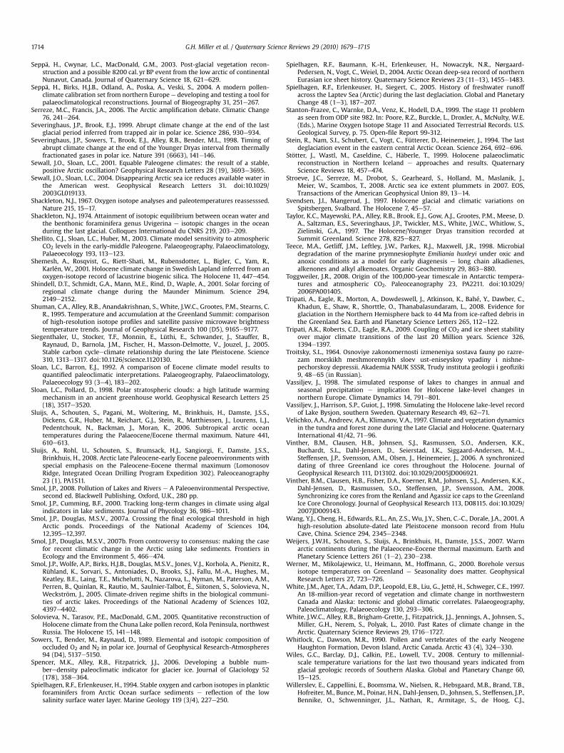
G.H. Miller et al. / Quaternary Science Reviews 29 (2010) 1679e17151714
Seppä, H., Cwynar, L.C., MacDonald, G.M., 2003. Post-glacial vegetation recon-struction and a possible 8200 cal. yr BP event from the low arctic of continentalNunavut, Canada. Journal of Quaternary Science 18, 621e629.
Seppä, H., Birks, H.J.B., Odland, A., Poska, A., Veski, S., 2004. A modern pollen-climate calibration set from northern Europe e developing and testing a tool forpalaeoclimatological reconstructions. Journal of Biogeography 31, 251e267.
Serreze, M.C., Francis, J.A., 2006. The Arctic amplification debate. Climatic Change76, 241e264.
Severinghaus, J.P., Brook, E.J., 1999. Abrupt climate change at the end of the lastglacial period inferred from trapped air in polar ice. Science 286, 930e934.
Severinghaus, J.P., Sowers, T., Brook, E.J., Alley, R.B., Bender, M.L., 1998. Timing ofabrupt climate change at the end of the Younger Dryas interval from thermallyfractionated gases in polar ice. Nature 391 (6663), 141e146.
Sewall, J.O., Sloan, L.C., 2001. Equable Paleogene climates: the result of a stable,positive Arctic oscillation? Geophysical Research Letters 28 (19), 3693e3695.
Sewall, J.O., Sloan, L.C., 2004. Disappearing Arctic sea ice reduces available water inthe American west. Geophysical Research Letters 31. doi:10.1029/2003GL019133.
Shackleton, N.J., 1967. Oxygen isotope analyses and paleotemperatures reassesssed.Nature 215, 15e17.
Shackleton, N.J., 1974. Attainment of isotopic equilibrium between ocean water andthe benthonic foraminifera genus Uvigerina e isotopic changes in the oceanduring the last glacial. Colloques International du CNRS 219, 203e209.
Shellito, C.J., Sloan, L.C., Huber, M., 2003. Climate model sensitivity to atmosphericCO2 levels in the early-middle Paleogene. Palaeogeography, Palaeoclimatology,Palaeoecology 193, 113e123.
Shemesh, A., Rosqvist, G., Riett-Shati, M., Rubensdotter, L., Bigler, C., Yam, R.,Karlén, W., 2001. Holocene climate change in Swedish Lapland inferred from anoxygen-isotope record of lacustrine biogenic silica. The Holocene 11, 447e454.
Shindell, D.T., Schmidt, G.A., Mann, M.E., Rind, D., Waple, A., 2001. Solar forcing ofregional climate change during the Maunder Minimum. Science 294,2149e2152.
Shuman, C.A., Alley, R.B., Anandakrishnan, S., White, J.W.C., Grootes, P.M., Stearns, C.R., 1995. Temperature and accumulation at the Greenland Summit: comparisonof high-resolution isotope profiles and satellite passive microwave brightnesstemperature trends. Journal of Geophysical Research 100 (D5), 9165e9177.
Siegenthaler, U., Stocker, T.F., Monnin, E., Lüthi, E., Schwander, J., Stauffer, B.,Raynaud, D., Barnola, J.M., Fischer, H., Masson-Delmotte, V., Jouzel, J., 2005.Stable carbon cycleeclimate relationship during the late Pleistocene. Science310, 1313e1317. doi:10.1126/science.1120130.
Sloan, L.C., Barron, E.J., 1992. A comparison of Eocene climate model results toquantified paleoclimatic interpretations. Palaeogeography, Palaeoclimatology,Palaeoecology 93 (3e4), 183e202.
Sloan, L.C., Pollard, D., 1998. Polar stratospheric clouds: a high latitude warmingmechanism in an ancient greenhouse world. Geophysical Research Letters 25(18), 3517e3520.
Sluijs, A., Schouten, S., Pagani, M., Woltering, M., Brinkhuis, H., Damste, J.S.S.,Dickens, G.R., Huber, M., Reichart, G.J., Stein, R., Matthiessen, J., Lourens, L.J.,Pedentchouk, N., Backman, J., Moran, K., 2006. Subtropical arctic oceantemperatures during the Palaeocene/Eocene thermal maximum. Nature 441,610e613.
Sluijs, A., Rohl, U., Schouten, S., Brumsack, H.J., Sangiorgi, F., Damste, J.S.S.,Brinkhuis, H., 2008. Arctic late Paleocene-early Eocene paleoenvironments withspecial emphasis on the Paleocene-Eocene thermal maximum (LomonosovRidge, Integrated Ocean Drilling Program Expedition 302). Paleoceanography23 (1), PA1S11.
Smol, J.P., 2008. Pollution of Lakes and Rivers e A Paleoenvironmental Perspective,second ed. Blackwell Publishing, Oxford, U.K., 280 pp.
Smol, J.P., Cumming, B.F., 2000. Tracking long-term changes in climate using algalindicators in lake sediments. Journal of Phycology 36, 986e1011.
Smol, J.P., Douglas, M.S.V., 2007a. Crossing the final ecological threshold in highArctic ponds. Proceedings of the National Academy of Sciences 104,12,395e12,397.
Smol, J.P., Douglas, M.S.V., 2007b. From controversy to consensus: making the casefor recent climatic change in the Arctic using lake sediments. Frontiers inEcology and the Environment 5, 466e474.
Smol, J.P., Wolfe, A.P., Birks, H.J.B., Douglas, M.S.V., Jones, V.J., Korhola, A., Pienitz, R.,Rühland, K., Sorvari, S., Antoniades, D., Brooks, S.J., Fallu, M.-A., Hughes, M.,Keatley, B.E., Laing, T.E., Michelutti, N., Nazarova, L., Nyman, M., Paterson, A.M.,Perren, B., Quinlan, R., Rautio, M., Saulnier-Talbot, É., Siitonen, S., Solovieva, N.,Weckström, J., 2005. Climate-driven regime shifts in the biological communi-ties of arctic lakes. Proceedings of the National Academy of Sciences 102,4397e4402.
Solovieva, N., Tarasov, P.E., MacDonald, G.M., 2005. Quantitative reconstruction ofHolocene climate from the Chuna Lake pollen record, Kola Peninsula, northwestRussia. The Holocene 15, 141e148.
Sowers, T., Bender, M., Raynaud, D., 1989. Elemental and isotopic composition ofoccluded O2 and N2 in polar ice. Journal of Geophysical Research-Atmospheres94 (D4), 5137e5150.
Spencer, M.K., Alley, R.B., Fitzpatrick, J.J., 2006. Developing a bubble num-beredensity paleoclimatic indicator for glacier ice. Journal of Glaciology 52(178), 358e364.
Spielhagen, R.F., Erlenkeuser, H., 1994. Stable oxygen and carbon isotopes in plankticforaminifers from Arctic Ocean surface sediments e reflection of the lowsalinity surface water layer. Marine Geology 119 (3/4), 227e250.
Spielhagen, R.F., Baumann, K.-H., Erlenkeuser, H., Nowaczyk, N.R., Nørgaard-Pedersen, N., Vogt, C., Weiel, D., 2004. Arctic Ocean deep-sea record of northernEurasian ice sheet history. Quaternary Science Reviews 23 (11e13), 1455e1483.
Spielhagen, R.F., Erlenkeuser, H., Siegert, C., 2005. History of freshwater runoffacross the Laptev Sea (Arctic) during the last deglaciation. Global and PlanetaryChange 48 (1e3), 187e207.
Stanton-Frazee, C., Warnke, D.A., Venz, K., Hodell, D.A., 1999. The stage 11 problemas seen from ODP site 982. In: Poore, R.Z., Burckle, L., Droxler, A., McNulty, W.E.(Eds.), Marine Oxygen Isotope Stage 11 and Associated Terrestrial Records. U.S.Geological Survey, p. 75. Open-file Report 99-312.
Stein, R., Nam, S.I., Schubert, C., Vogt, C., Fütterer, D., Heinemeier, J., 1994. The lastdeglaciation event in the eastern central Arctic Ocean. Science 264, 692e696.
Stötter, J., Wastl, M., Caseldine, C., Häberle, T., 1999. Holocene palaeoclimaticreconstruction in Northern Iceland e approaches and results. QuaternaryScience Reviews 18, 457e474.
Stroeve, J.C., Serreze, M., Drobot, S., Gearheard, S., Holland, M., Maslanik, J.,Meier, W., Scambos, T., 2008. Arctic sea ice extent plummets in 2007. EOS,Transactions of the American Geophysical Union 89, 13e14.
Svendsen, J.I., Mangerud, J., 1997. Holocene glacial and climatic variations onSpitsbergen, Svalbard. The Holocene 7, 45e57.
Taylor, K.C., Mayewski, P.A., Alley, R.B., Brook, E.J., Gow, A.J., Grootes, P.M., Meese, D.A., Saltzman, E.S., Severinghaus, J.P., Twickler, M.S., White, J.W.C., Whitlow, S.,Zielinski, G.A., 1997. The Holocene/Younger Dryas transition recorded atSummit Greenland. Science 278, 825e827.
Teece, M.A., Getliff, J.M., Leftley, J.W., Parkes, R.J., Maxwell, J.R., 1998. Microbialdegradation of the marine prymnesiophyte Emiliania huxleyi under oxic andanoxic conditions as a model for early diagenesis e long chain alkadienes,alkenones and alkyl alkenoates. Organic Geochemistry 29, 863e880.
Toggweiler, J.R., 2008. Origin of the 100,000-year timescale in Antarctic tempera-tures and atmospheric CO2. Paleoceanography 23, PA2211. doi:10.1029/2006PA001405.
Tripati, A., Eagle, R., Morton, A., Dowdeswell, J., Atkinson, K., Bahé, Y., Dawber, C.,Khadun, E., Shaw, R., Shorttle, O., Thanabalasundaram, L., 2008. Evidence forglaciation in the Northern Hemisphere back to 44 Ma from ice-rafted debris inthe Greenland Sea. Earth and Planetary Science Letters 265, 112e122.
Tripati, A.K., Roberts, C.D., Eagle, R.A., 2009. Coupling of CO2 and ice sheet stabilityover major climate transitions of the last 20 Million years. Science 326,1394e1397.
Troitsky, S.L., 1964. Osnoviye zakonomernosti izmeneniya sostava fauny po razre-zam morskikh meshmorennykh sloev ust-eniseyskoy vpadiny i nishne-pechorskoy depressii. Akademia NAUK SSSR, Trudy instituta geologii i geofiziki9, 48e65 (in Russian).
Vassiljev, J., 1998. The simulated response of lakes to changes in annual andseasonal precipitation e implication for Holocene lake-level changes innorthern Europe. Climate Dynamics 14, 791e801.
Vassiljev, J., Harrison, S.P., Guiot, J., 1998. Simulating the Holocene lake-level recordof Lake Bysjon, southern Sweden. Quaternary Research 49, 62e71.
Velichko, A.A., Andreev, A.A., Klimanov, V.A., 1997. Climate and vegetation dynamicsin the tundra and forest zone during the Late Glacial and Holocene. QuaternaryInternational 41/42, 71e96.
Vinther, B.M., Clausen, H.B., Johnsen, S.J., Rasmussen, S.O., Andersen, K.K.,Buchardt, S.L., Dahl-Jensen, D., Seierstad, I.K., Siggaard-Andersen, M.-L.,Steffensen, J.P., Svensson, A.M., Olsen, J., Heinemeier, J., 2006. A synchronizeddating of three Greenland ice cores throughout the Holocene. Journal ofGeophysical Research 111, D13102. doi:10.1029/2005JD006921.
Vinther, B.M., Clausen, H.B., Fisher, D.A., Koerner, R.M., Johnsen, S.J., Andersen, K.K.,Dahl-Jensen, D., Rasmussen, S.O., Steffensen, J.P., Svensson, A.M., 2008.Synchronizing ice cores from the Renland and Agassiz ice caps to the GreenlandIce Core Chronology. Journal of Geophysical Research 113, D08115. doi:10.1029/2007JD009143.
Wang, Y.J., Cheng, H., Edwards, R.L., An, Z.S., Wu, J.Y., Shen, C.-C., Dorale, J.A., 2001. Ahigh-resolution absolute-dated late Pleistocene monsoon record from HuluCave, China. Science 294, 2345e2348.
Weijers, J.W.H., Schouten, S., Sluijs, A., Brinkhuis, H., Damste, J.S.S., 2007. Warmarctic continents during the Palaeocene-Eocene thermal maximum. Earth andPlanetary Science Letters 261 (1e2), 230e238.
Werner, M., Mikolajewicz, U., Heimann, M., Hoffmann, G., 2000. Borehole versusisotope temperatures on Greenland e Seasonality does matter. GeophysicalResearch Letters 27, 723e726.
White, J.M., Ager, T.A., Adam, D.P., Leopold, E.B., Liu, G., Jetté, H., Schweger, C.E., 1997.An 18-million-year record of vegetation and climate change in northwesternCanada and Alaska: tectonic and global climatic correlates. Palaeogeography,Paleoclimatology, Palaeoecology 130, 293e306.
White, J.W.C., Alley, R.B., Brigham-Grette, J., Fitzpatrick, J.J., Jennings, A., Johnsen, S.,Miller, G.H., Nerem, S., Polyak, L., 2010. Past Rates of climate change in theArctic. Quaternary Science Reviews 29, 1716e1727.
Whitlock, C., Dawson, M.R., 1990. Pollen and vertebrates of the early NeogeneHaughton Formation, Devon Island, Arctic Canada. Arctic 43 (4), 324e330.
Wiles, G.C., Barclay, D.J., Calkin, P.E., Lowell, T.V., 2008. Century to millennial-scale temperature variations for the last two thousand years indicated fromglacial geologic records of Southern Alaska. Global and Planetary Change 60,15e125.
Willerslev, E., Cappellini, E., Boomsma, W., Nielsen, R., Hebsgaard, M.B., Brand, T.B.,Hofreiter, M., Bunce, M., Poinar, H.N., Dahl-Jensen, D., Johnsen, S., Steffensen, J.P.,Bennike, O., Schwenninger, J.L., Nathan, R., Armitage, S., de Hoog, C.J.,
G.H. Miller et al. / Quaternary Science Reviews 29 (2010) 1679e1715 1715
Alfimov, V., Christi, M., Beer, J., Muscheler, R., Barker, J., Sharp, M., Penkman, K.E.H., Haile, J., Taberlet, P., Bilbert, M.T.P., Casoli, A., Campani, E., Collins, M.J., 2007.Ancient biomolecules from deep ice cores reveal a forested SouthernGreenland. Science 317, 111e114.
Williams, C.J., Johnson, A.H., LePage, B.A., Vann, D.R., Sweda, T., 2003. Reconstruc-tion of tertiary metasequoia forests II. Structure, biomass and productivity ofEocene floodplain forests in the Canadian Arctic. Paleobiology 29 (2), 271e292.
Wohlfarth, B., Lemdahl, G., Olsson, S., Persson, T., Snowball, I., Ising, J., Jones, V.,1995. Early Holocene environment on Bjornoya (Svalbard) inferred frommultidisciplinary lake sediment studies. Polar Research 14, 253e275.
Wohlfahrt, J., Harrison, S.P., Braconnot, P., 2004. Synergistic feedbacks betweenocean and vegetation on mid- and high-latitude climates during the Holocene.Climate Dynamics 22, 223e238.
Wolfe, B.B., Edwards, T.W.D., Aravena, R., MacDonald, G., 1996. Rapid Holocenehydrologic change along boreal tree-line revealed by d13C and d18O in organiclake sediments, Northwest Territories, Canada. Journal of Paleolimnology 15,171e181.
Wolfe, B.B., Edwards, T.W.D., Aravena, R., Forman, S.L., Warner, B.G., Velichko, A.A.,MacDonald, G., 2000. Holocene paleohydrology and paleoclimate at treeline,north-central Russia, inferred from oxygen isotope records in lake sedimentcellulose. Quaternary Research 53, 319e329.
Wolfe, J.A., 1997. Relations of environmental change to angiosperm evolution duringthe Late Cretaceous and Tertiary. In: Iwatsuki, K., Raven, P.H. (Eds.), Evolutionand Diversification of Land Plants. Springer-Verlag, Tokyo, pp. 269e290.
Wuchter, C., Schouten, S., Coolen, M.J.L., Damsté, J.S.S., 2004. Temperature-depen-dent variation in the distribution of tetraether membrane lipids of marineCrenarchaeota e implications for TEX86 paleothermometry. Paleoceanography19 (4), PA4028.
Wuchter, W., Schouten, S., Wakeham, S.G., Sinninghe Damsté, J.S., 2005. Temporaland spatial variation in tetraether membrane lipids of marine Crenarchaeota inparticulate organic matter: implications for TEX86 paleothermometry. Paleo-ceanography 20, PA3013.
Zachos, J., Pagani, M., Sloan, L., Thomas, E., Billups, K., 2001. Trends, rhythms,and aberrations in global climate 65 Ma to present. Science 292 (5517),686e693.
Zachos, J.C., Dickens, G.R., Zeebe, R.E., 2008. An early Cenozoic perspective ongreenhouse warming and carbon-cycle dynamics. Nature 451 (7176),279e283.
Zazula, G.D., Froese, D.G., Schweger, C.E., Mathewes, R.W., Beaudoin, A.B., Telka, A.M., Harington, C.R., Westgate, J.A., 2003. Ice-age steppe vegetation in eastBeringia e tiny plant fossils indicate how this frozen region once sustainedhuge herds of mammals. Nature 423, 603e613.