technology selection and architecture optimization of in-situ
TRANSCRIPT

Technology Selection and Architecture Optimization of In-Situ Resource Utilization Systems
by
Ariane Chepko
B.S., Purdue University, 2006
Submitted to the Department of Aeronautics and Astronautics in partial fulfillment of the requirements for the degree of
Master of Science in Aeronautical and Astronautical Engineering
at the
MASSACHUSETTS INSTITUTE OF TECHNOLOGY
June, 2009
© Massachusetts Institute of Technology 2009. All rights reserved.
Signature of Author:………………………………………………………………………
Department of Aeronautics and Astronautics May 22, 2009
Certified by:………………………………………………………………………………...
Olivier de Weck Associate Professor of Aeronautics and Astronautics
and Engineering Systems Thesis Supervisor
Accepted by: ……………………………………………………………………………….
David L. Darmofal Associate Professor of Aeronautics and Astronautics
Associate Department Head Chair, Committee on Graduate Students
1
Technology Selection and Architecture Optimization of In-Situ Resource Utilization Systems
by
Ariane Chepko
Submitted to the Department of Aeronautics and Astronautics on May 22, 2009 in Partial Fulfillment of the Requirements
for the Degree of Master of Science in Aeronautical and Astronautical Engineering
Abstract
This paper discusses an approach to exploring the conceptual design space of large-scale, complex electromechanical systems that are technologically immature. A modeling framework that addresses the fluctuating architectural landscape (an inherent feature of developing technology systems) is applied to the design of a lunar in-situ resource utilization (ISRU) oxygen plant. Four optimization methods using genetic algorithms are compared on both a quadratic-based test function and the ISRU plant design with the goal of balancing the resources spent on exploiting individual architectures and exploring a broad selection of architectures. These include two dual-level approaches that address the discrete architecture design space differently from the continuous sizing design space and two combinatorial approaches that address both the discrete and continuous simultaneously. It was found that the single-level, combinatorial approaches worked better on the real-world ISRU case study, providing a balance between computation time spent on optimizing sizing and performance of each architecture and time spent searching a large number of architectures. For the ISRU architecture search, the single-level approaches on average covered ~300 architectures with ~5000 function evaluations. A heuristic-based dual-level approach covered ~266 architectures with ~5,500 function evaluations. A nested dual-level approach with gradient-based optimization of internal continuous variables nested within a heuristic search of discrete architecture variables would have required on the order of 300,000 function evaluations.
The ISRU plant architecture search found that a 300 kg mass ISRU oxygen plant can produce around 1500 kg O2/year, which is about the amount needed to sustain a crew of four for one year on the lunar surface. These preliminary results also indicate that ISRU plants exhibit an economy of scale of .78, implying that fewer, larger plants would be less costly than many smaller plants in building up a high production capacity. Thesis Supervisor: Olivier de Weck Title: Associate Professor of Aeronautics and Astronautics and Engineering Systems
2

Acknowledgements
In nearing the end of this long, thesis-writing process, there are a few people that deserve recognition and appreciation. I would like to thank my adviser, Olivier de Weck, for always letting me run off on whatever tangents to my research fancied me, and for supporting and encouraging me to work on the things I was interested in. I have learned much from him in the last two years. I would like to thank everyone on the NASA ISRU team, especially Kristopher Lee, Tom Simon, Edgardo Santiago-Maldonado, and Diane Linne. Kris put up with all my ups and downs and many detailed conversations about programming during my time at NASA, and I will forever appreciate his patience, encouragement, and support. Tom is a constant source of excitement and ideas, and I thank him for that. Eddie and Diane have provided many critiques, comments, and answers to my many questions over the last two years that have been invaluable in getting this project together. I would also like to thank Professor Crossley at Purdue for initiating the idea that this research is based on, providing feedback and advice from afar, and the support he has given me throughout my education. Thank you to Brendan Flynn for putting up with me for the last few months and for being you. Thank you also to all of my friends at MIT for making my graduate experience memorable and enjoyable, and to my friends far away who keep me motivated and remind me that our passion for space exploration will always burn strong. Lastly, I’d like to thank my parents and brothers for their love and un-ending support of all my endeavors. I’ll keep sailing on, Mom and Dad.
3
Table of Contents
Abstract ………………………………………………………………………………………. 2
Acknowledgements ……………………………………………………………………………3
Chapter 1: Introduction...............................................................................................................9
1.1 Motivation .........................................................................................................................9
1.2 Literature Review............................................................................................................13
1.2.1 Multidisciplinary Design Optimization ....................................................................13
1.2.2 Architecture Selection...............................................................................................14
1.2.3 Combinatorial Search Methods ................................................................................15
1.3 Gap Analysis ...................................................................................................................18
1.4 Summary .........................................................................................................................19
Chapter 2: The Architecture Search Problem...........................................................................20
2.1 System Modeling Framework Requirements..................................................................20
2.2 Functional Decomposition and Stable Interfaces............................................................21
2.3 Architecture Selection and Optimization ........................................................................23
2.3.1 Test Problem.............................................................................................................25
2.3.2 Full Enumeration ......................................................................................................27
2.3.3 GA Chromosome Representations and Single-Level Search Methods ....................29
2.3.4 Split-level Search Methods.......................................................................................32
2.3.5 Comparison of Results..............................................................................................34
Chapter 3: ISRU Lunar Oxygen Production ............................................................................41
3.1 ISRU Oxygen Production Processes...............................................................................41
3.1.1 Hydrogen Reduction .................................................................................................43
3.1.2 Carbothermal Reduction ...........................................................................................44
3.1.3 Molten Salt Electrolysis (Electrowinning) ...............................................................45
3.2 ISRU Architecture Trade Space......................................................................................45
Chapter 4: Applying Modeling Framework to the ISRU System Model .................................48
4.1 Functional Breakdown of ISRU Oxygen Plant...............................................................48
4.2 Implementation of ISRU System Architecture model ....................................................50
4.3 Application of Architecture Optimization ......................................................................52
4
4.3.1 Full Enumeration Attempts.......................................................................................54
4.3.2 Genetic Algorithm Methods .....................................................................................58
4.4 ISRU Architecture Search Results ..................................................................................63
4.4.1 GA Convergence History..........................................................................................63
4.4.2 Performance Comparison of Search Methods ..........................................................64
4.4.3 Architecture Search Across ISRU O2 Production Levels ........................................68
Chapter 5: Conclusions and Future Work ................................................................................72
5.1 Summary and Conclusions..............................................................................................72
5.2 Future Work ....................................................................................................................75
References…………………………………………………………………………………….77
Appendix…………………………………………………………………………………...…79
List of Figures………………………………………………………………………………….6
List of Tables…………………………………………………………………………………..7
Nomenclature ………………………………………………………………………………….8
5
List of Figures
Figure 1.1: Partial representation of system architecture discrete design…………………...10
Figure 1.2: Life cycle cost committed versus cost incurred per program phase ……….......11
Figure 1.3: Simple example of sGA chromosome structure………………………………..16
Figure 2.4: General functional decomposition showing AND/OR structure of system……21
Figure 2.5: Example illustrating model OR repositories and AND placeholders…………..23
Figure 2.6: Quadratic test function description……………………………………………..26
Figure 2.7: Design space of Quadratic Tree test problem…………………………………..27
Figure 2.8: Zoomed-in view of Quadratic Tree minimum fitness area……………………..28
Figure 2.9: Quadratic Tree optimal architecture……………………………………………29
Figure 2.10: Example of Nested-GA search coverage……………………………………...36
Figure 2.11: Example of Dual-Agent GA-ANT search coverage…………………………..37
Figure 2.12: Example of sGA architecture search coverage…………………………………37
Figure 2.13: Example of SLI GA architecture search coverage…………………………….38
Figure 2.14: Exploration vs Exploitation.................................................................................38
Figure 3.15: Hydrogen reduction schematic………………………………………………...43
Figure 3.16: Carbothermal reduction schematic…………………………………………….44
Figure 3.17: ISRU System Model Input/Output Structure………………………………….46
Figure 4.18: ISRU Oxygen System functional breakdown ………………………………...49
Figure 4.19: ModelCenter: top level of model ……………………………………………..51
Figure 4.20: ModelCenter: “OR” Level model repository of O2 Production Options……...51
Figure 4.21: Discrete architecture space of ISRU system included in optimization………..53
Figure 4.22: Example convergence history…………………………………………………64
Figure 4.23: ISRU Production Curve……………………………………………………….71
Figure 5.1: Time investment in architecture search with different modeling approaches…73
Figure A.1: ISRU SLI-GA architecture search coverage example……………………… ...79
Figure A.2: ISRU sGA architecture search coverage example……………………… …….80
Figure A.3: ISRU GAANT architecture search coverage example……………………… ..80
6

List of Tables
Table 1.1: Gap Analysis of Literature Review for Architecture Search Problem....................19
Table 2.1: Optimal choice in Quadratic Tree Problem.............................................................28
Table 2.2: Modified sGA Chromosome (real number representation).....................................30
Table 2.3: Compact Sex-Limited Inheritance sGA Chromosome............................................32
Table 2.4: GA Search Performance Averaged Over 40 and 100 Runs ....................................36
Table 3.1: Lunar Base Crew Oxygen Consumption.................................................................42
Table 4.1: Comparison of initial and final points in gradient optimizer runs……………...…55
Table 4.2: Computation Time Comparison ..............................................................................59
Table 4.3: sGA Chromosome for ISRU Architecture ..............................................................59
Table 4.4: SLI-GA Chromosome for ISRU Architecture Search.............................................60
Table 4.5: SLI-GA Run 3 Last Generation Diversity...............................................................64
Table 4.6: Overall Performance Comparison of GA methods .................................................65
Table 4.7 Results of ISRU Architecture Search for all Runs of SLI-GA.................................66
Table 4.8: Results of ISRU Architecture Search for all Runs of sGA .....................................66
Table 4.9: Results of ISRU Architecture Search for all Runs of GA-ANT .............................67
Table 4.10: Frequency of Variable Assignments for Top-Performing Architectures O2 = 1000
kg / yr .................................................................................................................................68
Table A.1: Table of Pareto Front Oxygen Plants .....................................................................79
7
Nomenclature
α = economy of scale C = investment cost f = objective function gi = inequality constraint k = scaling coefficient N = production quantity per unit time rp = penalty multiplier xi = design variable xLB = design variable lower bounds xUB = design variable upper bounds ECLSS = Environmental Control and Life Support Systems GA = Genetic Algorithm sGA = Structured Genetic Algorithm GA-ANT = Genetic Algorithm Ant Colony search ISRU = In-Situ Resource Utilization PEM = Proton Exchange Membrane (electrolysis system) SA = Simulated Annealing SLI = Sex-Limited Inheritance SO = Solid Oxide SQP = Sequential Quadratic Programming
8
Chapter 1: Introduction
1.1 Motivation
In any large-scale engineering system, the early stages of design involve making
numerous decisions that ultimately define the architecture of the system. These decisions
include technology selection for various subsystems and components, operational modes, and
configurations. For example, in the design of a spacecraft, there are propulsion technology
choices (liquid bi-propellant, electric, etc), power production technology choices (solar
panels, radio-isotope generators, etc.), and thermal control operational modes (active,
passive). Such alternatives can be expanded for almost every subsystem on the spacecraft. In
addition, each subsystem selection can also have a degree of variation involving technology
alternatives of the components within a subsytem (ex. hypergolic or cryogenic liquid
propellants, types of compressors) that further compound the decision space. Selections must
be made at every layer of the system in order to define an initial design for further analysis.
These selections form an architecture design space of discrete variables.
Compatibility constraints may exist between selections: choosing an electric
propulsion system may preclude certain power technologies because the combination would
be infeasible. Such constraints may help reduce the design space and are important to capture
correctly when initializing the problem. Figure 1.24 provides a partial representation of a
general system architecture space.
9
Figure 1.24 Partial representation of system architecture discrete design
Despite the presence of compatibility constraints, the initial design space of potential
system architectures is usually enormous. Common industry practice is to assess only a
handful of alternatives before down-selecting to a single choice to carry into detailed analysis
and subsequent development. Decisions are based on a set of requirements, engineering
judgment, historical background, and a limited number of initial trade studies (usually fewer
than ten architectures due to time and cost constraints [Mosher '99]). Subsystems are
designed concurrently and separately, with system engineers trying to piece them together to
make a feasible system. Any optimization usually occurs at the subsystem level or below;
however, because of interdependencies between subsystems, combining optimized
subsystems does not ensure an optimal overall system. If technical problems arise with the
chosen architecture later in the process, design changes are often difficult and expensive to
implement. Researchers agree that 50-80% of the total cost of a system is committed in the
first stages of design when there is the least amount of knowledge of the design (see Figure
1.25.) [Nadir '05]. This provides motivation for employing methods that can provide a wider
search of the design space at a moderate time and cost.
10
Figure 1.25 Life cycle cost committed versus cost incurred per program phase [Nadir '05].
For systems that incorporate new, immature technologies, there is little to no historical
background to draw from, and the information upon which base initial decisions is even more
limited. In these cases, analysis models of the new technologies need to be generated to help
assess and guide the design. This creates a two-pronged approach throughout the system-
level conceptual design process: analysis model development and hardware development.
Initial analyses guide the direction of early decisions, but as hardware tests and technology
development efforts progress, the fidelity of the analysis models is improved, providing better
information for system decisions. Depending on how the progress of development goes,
alternatives and options in the architecture decision space may be added or taken away. Thus
the design space landscape can fluctuate throughout the early design process.
As NASA prepares for a return to the Moon, a new set of technologies is being
developed that may help create a more sustainable approach to space exploration. Termed in-
situ resource utilization (ISRU), this concept involves using any resources available in the
lunar or space environment that would help reduce the quantity of supplies that must be
launched from Earth [Sanders '00]. Oxygen is a consumable resource used to supply crew air
and oxidizer in rocket propellant that can be extracted from the lunar regolith. Several
chemical processes can be used to produce oxygen from the metal oxides and glasses present
in lunar soil, but because there is no historical data to draw from in the design of these
11

systems, a detailed set of engineering models has been constructed to help assess the system-
level trades of some of these processes.
This presents the need for a way to explore large design spaces of architectures for
systems that incorporate immature technologies. Using Figure 1.24 as a guide, the problem
structure for exploring the architectural design space is determined. There are four main
aspects to this problem that must be addressed:
1. The hierarchical dependence of decisions.
2. Interdependencies of subsystems.
3. Compatibility constraints between selections of different branches.
4. Fluctuating architecture landscape due to developing technology options.
The hierarchical dependence of decisions is a natural feature that emerges from the
common engineering practice of decomposing a design problem into subsystems and
components. Here, subsystems can be considered blocks or modules that perform a certain
function for the system. They may require input from other subsystems in order to operate
(propulsion subsystem requires power from the power subsystem), but they provide specific
functionality that is not achieved by the other subsystems. In turn, subsystems can be broken
down into components that are combined to achieve the subsystem function. Components
will be the lowest level considered in the architecture design space. Hierarchical dependency
comes into play in that a choice for a particular component is only meaningful if its parent
subsystem technology option is also selected. Compatibility constraints are different from
hierarchical constraints in that they exist between options that have different parent branches.
Efficient enforcement of compatibility constraints precludes certain architectures from being
chosen, helping to avoid unnecessary analysis.
A particular system architecture is constructed by making allowed selections at each
decision point in the tree. Each subsystem must have a technology option selected. Analysis
models are then used to assess the ability of the architecture to meet the desired requirements
at a system level. Relevant sizing parameters may be optimized with tools that consider the
interdependencies of subsystems to provide the best possible performance estimate of each
particular architecture. An automated method of exploring the large design space is sought.
12
Because genetic algorithms excel at searching large, combinatorial design spaces, this study
will focus on ways to apply a genetic algorithm to this specific problem structure [Goldberg
'89].
1.2 Literature Review
1.2.1 Multidisciplinary Design Optimization
With the advancement of computing capabilities, there has been a growing effort both
from academia and some industries (mainly automotive and aerospace industries) to explore
more of the conceptual design space by using system modeling and optimization tools. This
enhanced exploration can help designers identify well-performing regions of the design space
that may otherwise be missed, allowing for more informed decision-making. Generally,
system models involve tying together models of individual subsystems or disciplines to
capture system-level trade-offs and interactions. A system model for an aircraft may involve
linking the analysis of the structures to an aerodynamics model and a propulsion model. The
resulting tool allows a designer to optimize the system as a whole and understand the effects
of one subsystem on another. This approach is known as Multidisciplinary Design
Optimization (MDO), and has been employed in engineering fields for the last twenty years,
with its usage increasing as computational power developed.
Numerous examples of system modeling and optimization exist in the literature,
including design of a blended-wing-body aircraft [Wakayama '00], communications satellites
[Hassan '03], and diesel engine exhaust treatment systems [Graff C. '06]. Most applications
of MDO tools focus on optimizing the performance of a single system architecture, such as
Wakayama’s optimization of a blended-wing body aircraft where a particular system
architecture is chosen, and the size and shape of the wing, angle of attack, etc are the design
variables.
As in the case of Wakayama’s application, many similar system models become very
complex both in terms of the individual analysis tools and their software construction and
integration. The NASA ISRU engineering models that are under development have seen
several design iterations [Steffen '07]. The original form of this system model consisted of
several versions of tightly integrated Excel Visual Basic analysis models. Each version of the
model captured one instantiation of a major system architecture (where major architectures
13
are the different combinations of high-impact alternatives at the higher levels of the
hierarchy).
This software framework approach is tedious when trying to explore an architecture
design space because each architecture is run manually, and a limited number of model
versions can be created. Additionally, problems arise in modeling systems that use sections
of analysis that are under constant revision. As one analysis component is updated, changes
often ripple through the rest of the system model, requiring extensive editing and time-
consuming maintenance by the model design experts. Depending on the original model
construction, updating a system or building a new architecture can take anywhere from
several hours to weeks worth of non-recurring engineering time. While some lower-level
alternative selections may be imbedded in a major architecture model, exploring these trade
studies manually can take up to an hour each for model set-up and internal optimization run-
times.
1.2.2 Architecture Selection
Other approaches do consider the discrete architecture space of conceptual design.
Graff and de Weck use a state-vector approach to model the effect of different component
technologies in diesel exhaust after-treatment systems [Graff C. '06]. However, in this
approach, only three architectures are considered and the component technologies are
arranged in a linear fashion along the exhaust stream: there is no hierarchical dependence.
Each architecture is individually optimized for performance according to system sizing
characteristics, and reconfiguration and comparison between different architectures is done
manually. For architecture spaces that are very large and complex, manual reconfiguration of
models is time consuming and allows room for human error. Even with computer
automation, the number of possible architectures can easily explode and make full
enumeration infeasible, generating the need for a heuristic search technique like genetic
algorithms.
Mosher automates the search through large architecture spaces for spacecraft design
with the SCOUT tool [Mosher '99]. This systems engineering tool uses parametric
relationships to model the various spacecraft subsystems. It then employs a genetic algorithm
to search through and optimize a set of discrete technology option variables. Only the
14

discrete selection variables are included in the optimization. Because the models use
parametric relationships, continuous sizing parameters (such as solar array area) are not
included in the analysis. This limits the fidelity of analysis but does allow for faster
computation times. The major drawback to the use of parametric models for the purposes of
this paper is that these models are based on historical data. New systems require more
detailed analysis models to characterize performance.
Some issues are encountered with SCOUT in handling compatibility constraints. One
compatibility constraint exists in the trade space and when met by the genetic algorithm, a
repair technique is used to try modifying the infeasible solution and force it into feasibility.
This approach is found to be difficult and computationally expensive, but the author notes that
no clear alternative approach is apparent. SCOUT also does not handle decision variables that
are hierarchically connected.
Simmons developed a system architecting strategy called Architecture Decision
Graphs (ADG) [Simmons '08]. This strategy aids planners in defining the initial architecture
space and then searching for sets of feasible architectures. It helps in understanding how high
level decisions are connected, but it is enumerative, does not explicitly model hierarchical
decisions, and does not involve the detail of analysis necessary for system optimization. This
approach is more applicable to even earlier stages of the system design than this paper is
addressing.
1.2.3 Combinatorial Search Methods
Two studies have been found that address optimization and selection of architectures
with hierarchical decisions spaces. Rafiq, Mattews, and Bullock applied a structured genetic
algorithm (sGA) to conceptual design of office building structures [Rafiq '03]. The problem
creates a hierarchical breakdown of the building load-bearing system alternatives to map into
the sGA chromosome. Optimization is carried out with discrete decision variables that define
types of building frame, floor systems, and material selections and continuous variables that
further describe each option: grid dimensions, spans, and building dimensions.
While there is a hierarchical connection between discrete variables (ex. one set of
floor systems is only relevant to one type of frame), there is no subsystem interdependence.
The problem is structured as an OR tree, where a distinct configuration follows one branch
15
down the tree, only spreading into multiple paths at the “leaves” which represent relevant
continuous variables. The representation of architectures that exhibit subsystem
interdependence follows an AND/xOR tree, where multiple branches corresponding to
subsystems must be followed for each architecture with exclusive OR choices made for each
subsystem.
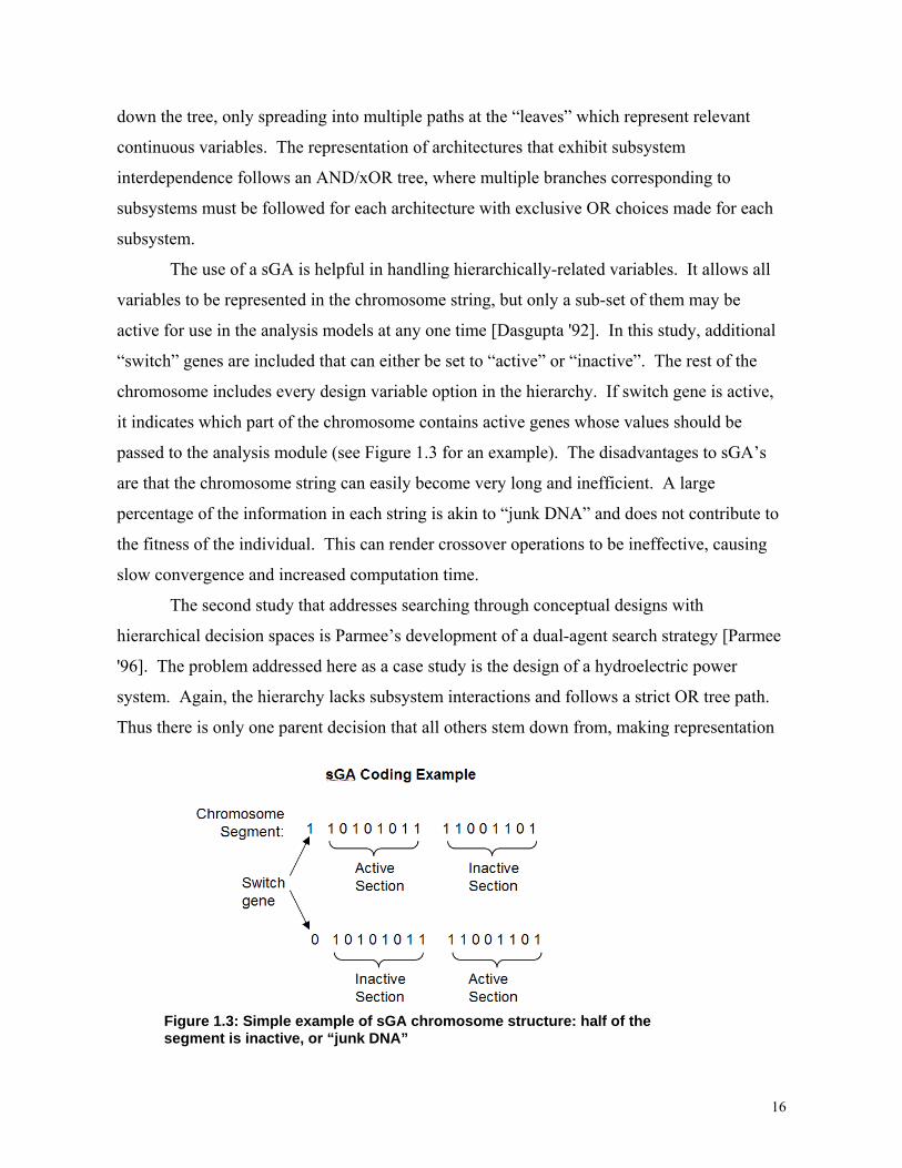
The use of a sGA is helpful in handling hierarchically-related variables. It allows all
variables to be represented in the chromosome string, but only a sub-set of them may be
active for use in the analysis models at any one time [Dasgupta '92]. In this study, additional
“switch” genes are included that can either be set to “active” or “inactive”. The rest of the
chromosome includes every design variable option in the hierarchy. If switch gene is active,
it indicates which part of the chromosome contains active genes whose values should be
passed to the analysis module (see Figure 1.3 for an example). The disadvantages to sGA’s
are that the chromosome string can easily become very long and inefficient. A large
percentage of the information in each string is akin to “junk DNA” and does not contribute to
the fitness of the individual. This can render crossover operations to be ineffective, causing
slow convergence and increased computation time.
The second study that addresses searching through conceptual designs with
hierarchical decision spaces is Parmee’s development of a dual-agent search strategy [Parmee
'96]. The problem addressed here as a case study is the design of a hydroelectric power
system. Again, the hierarchy lacks subsystem interactions and follows a strict OR tree path.
Thus there is only one parent decision that all others stem down from, making representation
Figure 1.3: Simple example of sGA chromosome structure: half of the segment is inactive, or “junk DNA”
16
in an algorithm simpler, reducing the size of the decision space, and not addressing cross-
subsystem compatibility constraints. The problem includes a set of continuous variables for
each architecture option that are also part of the optimization. This helps to ensure fair
comparison between architectures by searching for the best sizing configuration for each.
The goal of this study is to find a method that samples across a wide enough range of
the hierarchy to identify high-performance regions. If an algorithm settles too early on one
architecture, it will spend a larger percentage of time on optimizing the continuous variables
of that combination instead of searching through the broader architecture space. Two search
methods are compared in this study: a sGA that employs a different mutation rate for the
discrete parameters and the continuous parameters, and a dual-agent approach that combines
aspects of a simple GA and aspects of an Ant Colony search.
The main premise behind each method is to separate how the discrete, architecture
variables are evolved from the evolution of the continuous, architecture-specific sizing
variables. This prevents the loss of “good DNA” for sizing parameters during crossover
between discrete configurations; a set of high-fitness sizing parameters for one architecture
may be poor for a different architecture, so if the two “types” of DNA are mixed in crossover,
information may be lost.
As in the case of Rafiq, the problem formulation for the sGA method includes as a
variable every option in the hierarchy, along with repeated sets of continuous variables for
each type of architecture (ex. in the hydropower plant case study, all architectures have a
sizing parameter “dam height”, but instead of being modeled in the chromosome as a single
variable, there is a “dam height” variable for every architecture possibility—almost twenty
different “dam height” genes). This approach is the solution to handling hierarchical
compatibility constraints for both the Parmee and the Rafiq studies. It leads to the main
disadvantage of structured GA’s in that for more complex hierarchies, the chromosome string
grows exponentially.
The dual-agent GA-ANT colony technique allows a simpler parameter representation
by fully separating the evolutionary operations that are applied to the two sets of variables.
The results reported are promising for applications to searching architecture hierarchies.
However, this approach does not address subsystem interdependence or the existence of
compatibility constraints.
17
An approach that is applicable to compatibility constraints is the concept of “sex-
limited inheritance” proposed by Crossley. This method draws an analogue to the sex-limited
inheritance effect in biological systems, a familiar example being male-pattern baldness
[Crossley '95]. The gene that causes baldness in men can be carried by women, but is
generally not expressed. It requires the presence of the sex gene activated as male to express
the baldness gene. This is similar to the sGA representation, but the difference lies in the
chromosome implementation. Here, the assignment of a previous gene changes how the sex-
limited gene is expressed. This in effect dynamically changes the domain of the variable.
The implementation requires more intelligence in the decoding process, but in the case
of cross-branch compatibility constraints it will prevent the creation and evaluation of
infeasible architectures without added computation time.
1.3 Gap Analysis
The literature review reveals that various aspects of the AND/xOR hierarchical
architecture search problem have been addressed, but no approach tackles all aspects of the
problem. MDO system modeling techniques handle integrating multiple subsystems, but
none of the studies reviewed look at the hierarchical architecture space. Methods that
incorporate hierarchies of discrete variables lack the subsystem integration. Compatibility
constraint methods have been effectively used for rotorcraft optimization, but have not been
applied to a hierarchical problem. None of the studies address the issues specific to
developing technologies of modeling a varying architecture landscape.
18
Table 1.1: Gap Analysis of Literature Review for Architecture Search Problem
Previous Work: Hierarchical Dependence
Subsystem Interdependence
Compatibility Constraints
Fluctuating Architecture Design Space (New Technologies)
MDO System Modeling ([Wakayama '00], [Wilcox '03])
NO YES NO NO
Diesel Exhaust Systems [Graff C. '06] NO YES NO NO
Spacecraft Concept Selection and Design- SCOUT tool [Mosher '99]
NO YES YES NO
Conceptual Building Design [Rafiq '03] YES NO NO NO
Dual-Agent Search in Hydroelectric Power Systems [Parmee '96]
YES NO NO NO
Sex-Limited Inheritance [Crossley '95] NO YES YES NO
1.4 Summary
The remainder of this paper discusses the development of a system modeling
framework that enables searching through a large architecture design space for optimization
of sizing parameters and system technology options. This framework is discussed in Chapter
2 and applied to a simplified test problem. It captures the hierarchical nature of the
technology selection problem as well as subsystem interactions. Compatibility constraints are
accounted for, and the framework is designed specifically to accommodate the modeling
efforts of developing technologies. Four architecture search and optimization methods are
presented, and their performance is compared on the test problem. Chapter 3 provides an
overview of ISRU technologies and ISRU model development, and Chapter 4 presents the
application of the modeling framework and optimization methods to ISRU lunar oxygen plant
design.
19
Chapter 2: The Architecture Search Problem
2.1 System Modeling Framework Requirements
In order to explore the architecture space of a system that uses immature technologies,
a system model must be built that captures all the relevant subsystem and component
technology alternatives. Because technology alternatives for any given subsystem are often
very different from each other, each one can be considered as a separate analysis model. The
main issue that is encountered with system models of developing technologies is that the
models themselves are frequently changing. When these analyses are included as a part of a
tightly connected, unstructured system model, updates to the analysis models also usually
require extensive updates to the rest of the system model or manual re-connection processes
that leave room for human error. In large, complex system models, such errors may never be
found.
To avoid these issues and allow for searching through the architecture design space, a
modeling framework has been developed that provides the necessary structure to the system
model. The goal of the framework is to build a system model that exhibits the following
features:
1. Reconfigurability: to enable easy transitioning of the system model between technology
alternatives to represent different system architectures.
2. Flexibility: to allow for future expansion of the model and addition of new technology
alternatives or updating of old analysis models.
3. Optimization: methods that examine both the parameters specific to single system or
subsystem designs as well as the effects of different combinations of technologies.
The system model must be constructed in a manner that allows access to the sizing and
performance parameters that are internal to each technology model as well as control over
which technology model is plugged into the rest of the system. In this way, the models
themselves become variables in the architecture search of the system model. This structure
will enable both the assessment of point designs and a wide architecture search.
20

2.2 Functional Decomposition and Stable Interfaces
The key to the system modeling framework is to follow a functional decomposition of
the system. Breaking a system down in this manner can be somewhat intuitive, but the
primary result is that it allows the modeler to define the stable interfaces and basic functions
that must always be present to comprise the particular type of system being analyzed. Figure
2.1 illustrates a general functional decomposition, following the same concept presented in
Chapter 1.
Decomposing the system into its constituent elements reveals a pattern in the levels of
the hierarchy. Each alternating level consists of either subsystems whose functions must be
combined together to create their parent function (“AND” levels), or a set of choices from
which only one is needed to achieve its parent function (“OR” levels- which act as the
Boolean exclusive, xOR).
The system model is structured according to this decomposition with constant
interfaces defined for each block. Each block can be represented by a standalone analysis
model. The “xOR” levels act as repositories for the different model alternatives that perform
Figure 2.1: General functional decomposition showing AND/OR structure of system.
21
the function described by the parent block (ex. all technology alternatives for Subsystem 1 are
contained in its xOR repository). The “AND” levels act as placeholders, defining the basic
inputs and outputs needed for each AND function. By defining the stable interfaces
throughout the entire system, a “black box” approach to the analysis models can be adopted,
creating a “plug and play” model architecture at multiple levels.
If a new option for Component 1 has been developed, it can be plugged in and tested
in the system framework, or, on a higher level, a complete Subsystem 1 option model can be
added to the framework (the options at xOR1 do not necessarily have to be expanded into
components). The internal analysis of the Component 1 option designs may be very different
as long as they each provide the same basic required inputs and outputs to the system model
that define the parent function according to its stable interface.
With these repositories and knowledge of compatibility constraints, the system model
contains all potential system configurations. The inputs and outputs of the models are linked
together, choosing one option at each “OR” level, to form an end-to-end system model
configuration. Because the inputs and outputs of each subsystem and component function are
defined in a stable interface, the “plugging-in” of different model options can be automated:
the computer can be told what variables to look for, and where to send that information. This
is what creates a reconfigurable, flexible framework. Because the analysis path can be
directed by selecting OR options, the hierarchical constraints of the technology selections are
automatically handled: an option for a component will only have meaning if its parent
subsystem option is also selected to tie in to the model. If a different subsystem is selected,
that option and its subsequent component selections will be the models included in the
analysis path. In this manner, the hierarchical constraints flow from the top down.
While links at OR levels are made and broken for every architecture of the system, the
ties between AND level placeholders remain constant. These ties pass information about
subsystem interdependence. If a spacecraft propulsion subsystem is modeled with a power
subsystem, the propulsion subsystem may have an electric propulsion option and a liquid
propellant option. Regardless of how the analysis for each option proceeds, they both must
provide as outputs power requirements and propulsion performance. The selected option
connects this information to the Propulsion subsystem placeholder. The AND level
connections between power and propulsion then include 1. the power requirement of the
22
propulsion system (passed to the power subsystem placeholder), and 2. the mass of the power
system is returned to the propulsion system (which may require iteration between the two to
resolve). Thus, various options can be included in the analysis path, but the basic interactions
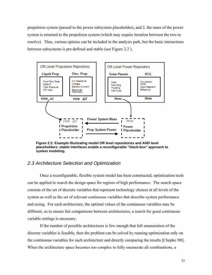
between subsystems is pre-defined and stable (see Figure 2.2 ).
Figure 2.2: Example illustrating model OR level repositories and AND level placeholders: stable interfaces enable a reconfigurable “black-box” approach to system modeling.
2.3 Architecture Selection and Optimization
Once a reconfigurable, flexible system model has been constructed, optimization tools
can be applied to search the design space for regions of high performance. The search space
consists of the set of discrete variables that represent technology choices at all levels of the
system as well as the set of relevant continuous variables that describe system performance
and sizing. For each architecture, the optimal values of the continuous variables may be
different, so to ensure fair comparisons between architectures, a search for good continuous
variable settings is necessary.
If the number of possible architectures is few enough that full enumeration of the
discrete variables is feasible, then the problem can be solved by running optimization only on
the continuous variables for each architecture and directly comparing the results [Chepko '08].
When the architecture space becomes too complex to fully enumerate all combinations, a
23
search technique must be employed that can find good architectures. The optimization tools
then need to handle a mix of continuous and discrete variables, compatibility constraints
between technology selections, and the potential of non-linear design spaces.
The first approach considered for this search problem was to treat it as a dual-level,
nested optimization problem where the continuous variables would be handled by an inner-
level optimization routine (using gradient-based, non-linear optimization tools), and the outer-
level would optimize only the discrete, architecture variables. With this approach, every
architecture assessed by the outer-level routine would run an inner-level sizing optimization
to find the best set of continuous parameters for that architecture. To handle the discrete
variables, a genetic algorithm was selected. This split-level approach may help the discrete-
space search by ensuring good architecture comparisons, but if the continuous space search is
computationally expensive, it may result in the whole search being too slow.
Another split-level approach that separates the discrete and continuous variables stems
from the work of Parmee discussed in Chapter 1. With this method, continuous variables are
searched independently in an inner-level optimization problem but not necessarily to
completion or optimality with each search. This intends to move the continuous design space
towards better designs without spending too much computation time chasing optimality at
each evaluation of an architecture. Over the course of the whole search, both the discrete and
continuous sets improve together.
The second main type of search is to consider the discrete and continuous variables
together in one combinatorial optimization problem formulation. This results in a single-level
search with a space the size of the combined discrete and continuous search spaces. Initial
intuition with this approach senses that it may be difficult to find sets of well-performing
continuous variables in such a wide design space. Two genetic algorithm chromosome
representations were tested with this single-level approach and compared with the two split-
level approaches.
A genetic algorithm was chosen for the discrete and combinatorial search in each of
the four methods because it provides a global search method that does not require gradients
for convergence and can handle both discrete and continuous variables. Genetic algorithms
are evolutionary search techniques that mimic Darwin’s Theory of Natural Selection
[Goldberg '89]. The design variables are coded as a string of binary numbers, creating a
24
chromosome that is used to obtain one function evaluation. A population of chromosomes is
generated and designs are competed against one another using their function evaluations as
criteria. Concepts like inheritance, selection, crossover, and mutation are incorporated into
the execution of the genetic algorithm, with mutation providing a probabilistic trigger that
keeps the search from settling on local minima and helps the search sample the entire design
space.
In designing a GA representation to handle the architecture search problem, it must
accommodate the hierarchically-connected discrete variables, compatibility constraints
between discrete variables, and the AND-OR structure of the architecture space. Two GA
chromosome representations have been developed to address these various aspects. The
performance of the two single-level and the two split-level GA methods is compared on a
simplified test problem.
2.3.1 Test Problem
2.3.1.a Designing a test function
Developing a test function for a genetic algorithm is not a straightforward task. It must
be easily solved via another method to determine and compare GA performance, but it must
also exhibit the difficult traits of a problem that usually warrant use of a GA. Watson et al
discuss constructing hierarchical test functions for genetic algorithms that are designed to test
the building block theory of how GA’s work [Watson '98]. These functions carry several
analogues to the architecture search problem, and their construction rules were used in
designing the architecture test problem. The functions consist entirely of binary variables and
are defined to be hierarchically decomposable into smaller sub-problems that are non-
separable. Non-separable sub-problems imply that the optimal solution of one sub-problem is
dependent upon the solution of another: there is interdependency between sub-problems. This
is built into the binary test functions by incorporating logic that sets a good fitness to a set of
sub-problems only if the assignment of all sub-problems are equal to 1 or all equal to 0. Thus
individual assignment of 0 or 1 may both be good, depending on how neighboring variables
are set. This concept ripples recursively through the hierarchy, with fitness values of sub-
problems being combined to create higher-level fitnesses, until it reaches the top level.
25
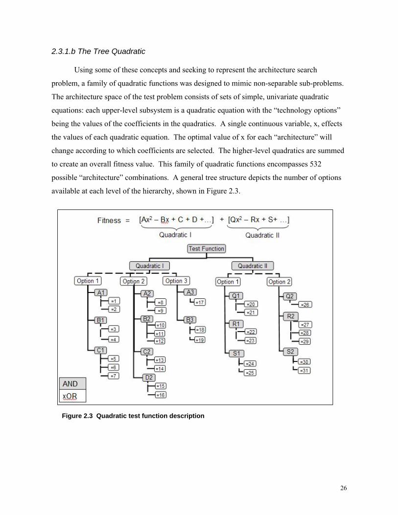
2.3.1.b The Tree Quadratic
Using some of these concepts and seeking to represent the architecture search
problem, a family of quadratic functions was designed to mimic non-separable sub-problems.
The architecture space of the test problem consists of sets of simple, univariate quadratic
equations: each upper-level subsystem is a quadratic equation with the “technology options”
being the values of the coefficients in the quadratics. A single continuous variable, x, effects
the values of each quadratic equation. The optimal value of x for each “architecture” will
change according to which coefficients are selected. The higher-level quadratics are summed
to create an overall fitness value. This family of quadratic functions encompasses 532
possible “architecture” combinations. A general tree structure depicts the number of options
available at each level of the hierarchy, shown in Figure 2.3.
Figure 2.3 Quadratic test function description
26
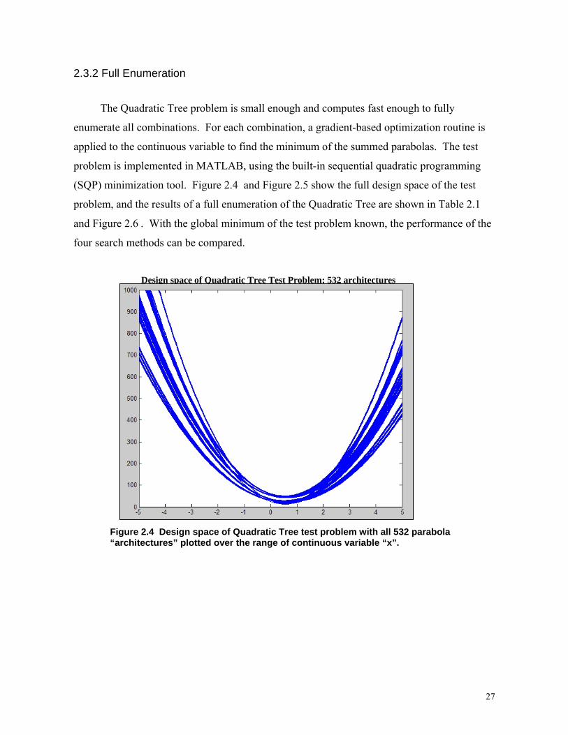
2.3.2 Full Enumeration
The Quadratic Tree problem is small enough and computes fast enough to fully
enumerate all combinations. For each combination, a gradient-based optimization routine is
applied to the continuous variable to find the minimum of the summed parabolas. The test
problem is implemented in MATLAB, using the built-in sequential quadratic programming
(SQP) minimization tool. Figure 2.4 and Figure 2.5 show the full design space of the test
problem, and the results of a full enumeration of the Quadratic Tree are shown in Table 2.1
and Figure 2.6 . With the global minimum of the test problem known, the performance of the
four search methods can be compared.
Design space of Quadratic Tree Test Problem: 532 architectures
Figure 2.4 Design space of Quadratic Tree test problem with all 532 parabola “architectures” plotted over the range of continuous variable “x”.
27
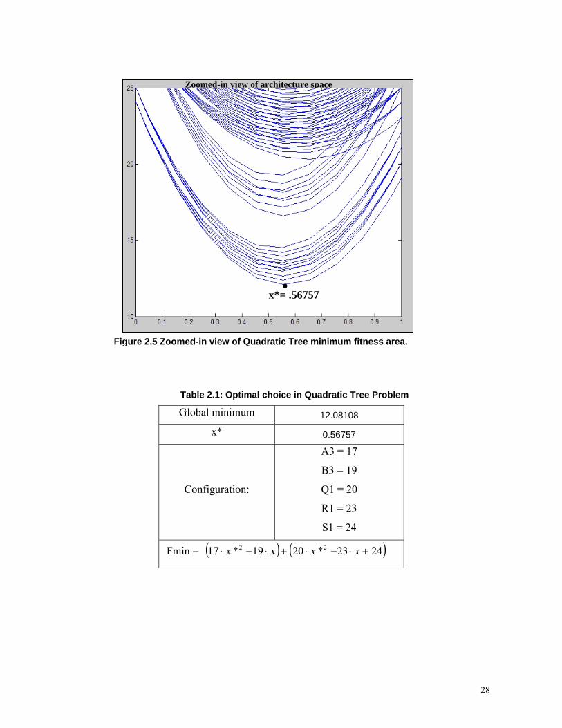
Zoomed-in view of architecture space
x*= .56757 •
Figure 2.5 Zoomed-in view of Quadratic Tree minimum fitness area.
Table 2.1: Optimal choice in Quadratic Tree Problem
Global minimum 12.08108
x* 0.56757
Configuration:
A3 = 17
B3 = 19
Q1 = 20
R1 = 23
S1 = 24
Fmin = ( ) ( )2423*2019*17 22 +⋅−⋅+⋅−⋅ xxxx
28
e
2.3.3 GA
2.3.3.a M
The
GA. In th
chromoso
continuou
from the s
used to re
gene for e
continuou
four extra
gene has 1
problem,
cumberso
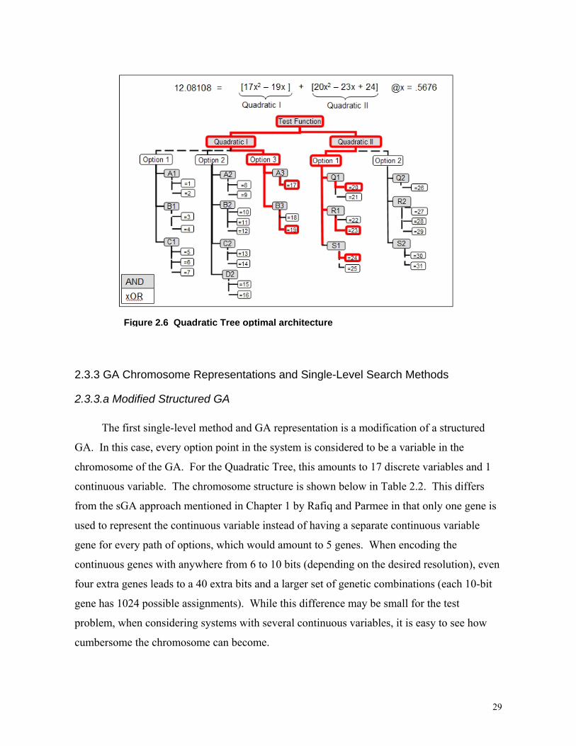
Figure 2.6 Quadratic Tree optimal architectur
Chromosome Representations and Single-Level Search Methods
odified Structured GA
first single-level method and GA representation is a modification of a structured
is case, every option point in the system is considered to be a variable in the
me of the GA. For the Quadratic Tree, this amounts to 17 discrete variables and 1
s variable. The chromosome structure is shown below in Table 2.2. This differs
GA approach mentioned in Chapter 1 by Rafiq and Parmee in that only one gene is
present the continuous variable instead of having a separate continuous variable
very path of options, which would amount to 5 genes. When encoding the
s genes with anywhere from 6 to 10 bits (depending on the desired resolution), even
genes leads to a 40 extra bits and a larger set of genetic combinations (each 10-bit
024 possible assignments). While this difference may be small for the test
when considering systems with several continuous variables, it is easy to see how
me the chromosome can become.
29
Table 2.2: Modified sGA Chromosome (real number representation)
Genes: Option A1 B1 C1 A2 B2 C2 D2 A3 B3 Option Q1 R1 S1 Q2 R2 S2 x#
choices 3 2 2 3 2 3 2 2 1 2 2 2 2 2 1 3 2 1024
Cont. Var.
Quadratic II Quadratic I
2.3.3.b Subsystem Interdependence and Compatibility Constraints
All GA implementations for this problem include subsystem interdependence by
concatenating strings of hierarchically-related genes. In the function evaluation process, the
chromosome is decoded by checking the setting of the “Option” genes to determine which
proceeding genes to activate. One path for each “Subsystem” is activated and included in the
analysis path.
Compatibility constraints are handled at the same point in the decoding process by
dynamically limiting the domain of the constrained variable. Compatibility constraints as
considered in this problem are by definition bi-directional. For example, if a choice of C1=5
is deemed incompatible with a choice of Q1=20, then choosing C1=5 will only allow
selection of Q1=21. Reversing the order of assignment, selecting Q1=20 allows only C1=6 or
C1=7. These two implementations of the constraint are equivalent, thus only one direction
needs to be checked in the decoding process to ensure feasibility and coverage of all
allowable combinations.
During decoding, if a gene is flagged to have a compatibility constraint, a check is
performed to test if its constraint-pair variable has already been assigned earlier in the
decoding process. If it has, the domain of the gene assignment is constrained to feasible
solutions, and the gene assignment is mapped into the allowed domain. For example, at gene
Q1, the original domain size is equal to 2, the domain being [20, 21]. If C1 has been set to 5
earlier in the chromosome, the new domain size of Q1 is equal to 1, the limited domain being
[21]. If the value assigned by the sGA to Q1 equals 2, this is now outside of the allowed
domain and is mapped back in via the following logic:
30
if gene assignment > new domain
value = gene assignment – (old domain – new domain)
else
value = gene assignment
end
2.3.3.c Integer Binary Decoding: Extra-Choices for Odd-Valued Domains
Another issue that must be handled in the discrete variable decoding process involves
variables that have odd-numbered domain sizes. Because all discrete variables are integer
valued, the resolution for binary encoding must be set to 1. Binary encoding always has an
even number of options equal to 2bits. A domain size of 3 then requires 2 bits (equal to 4
options) to fully cover, leaving one “extra bit”. This must be shuffled back into the allowable
domain by “double-assigning” some values in the gene. Thus, for the gene representing C1, if
the gene = 1, 2 or 3, C1 = 5, 6, or 7. If the gene is set to 4, this is mapped back to C1=7. This
approach to handling extra binary-induced choices causes some assignments to have a higher
probability of assignment, but this is a factor that the GA navigates through with the selection
operator.
2.3.3.d Compact sGA: Sex-Limited Inheritance (SLI) approach
The second single-level search method and GA chromosome representation
incorporates the concept of sex-limited inheritance discussed in Chapter 1. In this approach,
the chromosome is compacted by having a genotype that can express multiple phenotypes for
each subsystem. The chromosome section for Subsystem I consists of one gene that
represents the subsystem option choice followed by a number of genes that is equal to the
maximum number of components for any of the subsystem options. In the Quadratic Tree
problem, for the Quadratic I subsystem, there is a maximum of 4 components, which in the
problem are coefficient choices. Thus, in the compact SLI encoding, the subsystem can be
represented with 5 genes.
The component genes can be expressed three different ways, depending on which value
is selected for the option gene. If Option 1 is selected, the B gene maps to B1 with a domain
size equal to 2. If Option 2 is selected, B2 is activated with a domain size of 3. Domain sizes
31

may be different across options, so the upper bound of the gene is set to the maximum domain
size of the options. This requires active domain limiting and gene value mapping which is
handled with the same process as the compatibility constraints and extra binary choices, as
described in Section 2.3.4. There may still be completely inactive genes due to differences in
numbers of components for options of a particular subsystem. In Quadratic I, Option 2 has 4
components while Options 1 and 3 have fewer. In the cases when the Option gene is set to 1
or 3, the D or C and D genes will not be expressed in the phenotype (these are sex-limited,
dictated by the Option gene).
With the SLI approach, the entire problem can be represented with 10 genes rather than
the 18 genes of the normal sGA. This difference will grow with more complex system
hierarchies. Table 2.3 depicts the SLI chromosome representation.
Table 2.3: Compact Sex-Limited Inheritance sGA Chromosome
Gene: Option A B C D Option Q R S xMax #
choices 3 2 3 3 2 2 2 3 2 1024
Min # - 1 2 2 1 0 - 2 2 choices -
2.3.4 Split-level Search Methods
2.3.4.a Nested GA-Gradient-Based Hybrid
The most intuitive approach to the architecture search problem involves applying a GA
to the outer-level discrete, architecture variables with a classic, gradient-based method
operating on the continuous variables for each function evaluation of the outer-level GA. In
this approach, the compact SLI chromosome representation structure from Section 2.3.3.d is
employed on the outer level, and the same SQP algorithm used in the full enumeration runs is
applied to the inner level.
Quadratic I Cont. Var. Quadratic II
32

2.3.4.b Dual-Agent GA
2.3.4.b.i Exploration versus Exploitation
The second split-level approach is based on the work of Parmee’s dual-agent GAANT
algorithm [Parmee '96]. This method diverges from the simple GA operators by splitting
genetic operators applied to the continuous variables from operators applied to the discrete
architecture variables. The goal is to maintain diversity in the search through architectures to
try to find several architectures that have good fitnesses, rather than spending the majority of
computation time on tweaking the continuous variables of one, best-performing architecture.
In conceptual design development, this hits on the competing ideas of exploration and
exploitation. A high degree of exploration of the design space is desirable to search for
different types of solutions, but this is always countered by the degree of exploitation (depth
or fidelity of analysis) invested in each solution [March '91]. One can perform a fast search
across many design configurations using very low-fidelity analysis models, but the utility of
the results are then questionable if the level of analysis is too course. Investing in higher-
fidelity models usually reduces the amount of exploration achievable due to computation
times. This paper is directed at balancing these two forces.
2.3.4.b.ii Dual-Agent Algorithm
The dual-agent algorithm uses the same compacted chromosome coding scheme as the
SLI-sGA method. The theory behind the approach is that in a simple GA, crossover occurring
across the entire chromosome may cause good genetic information in the continuous variables
to be lost if crossed to an architecture that performs poorly at those settings. If simple GA
operators (selection, crossover, and mutation) are only applied to continuous variables within
a “species” or related family of architectures, the high-fitness combinations can be found
without disruption. This develops an architecture to its fitness potential—exploitation.
Exploration across species is achieved with another agent, in this case an adaptation of
Ant Colony Search operations [Parmee '96]. Continuous variables are modified with the
simple GA for a set number of generations, n, while the discrete architecture paths are held
constant. Then, the performance of each species over the last cycle of n generations is
averaged and compared to the last generation average fitness. The best species are copied
straight to the next generation of architectures, the worst species are eliminated, and the
33
average-performing species undergo mutation. The evaluation of “best”, “worst”, and
“average” differ in this paper from Parmee’s approach. Here, relative fitness of the species is
determined by Eqn 2.1 below.
)_()__(__
lastgenfitallspeciesmeangensnspeciesfitmeanfitrelativespecies = (2.1)
Where:
species_relative_fit = relative fitness of each species. speciesfit_n_gens = mean fitness of each species for each of n generations. allspeciesfit_lastgen = fitnesses of entire last generation of cycle.
If the species fitness is less than 10% of the last generation mean, it is copied into the
“best” pool. If the species fitness is more than 200% of the last generation mean, the species
is eliminated. Species in-between the two cut-off points are mutated with a probability of .07.
If the population size is reduced by the elimination of species, new species are randomly
generated to fill the population. Between the fill-in and mutation, adequate diversity can be
maintained while the fitness thresholds provide selection pressure.
2.3.5 Comparison of Results
The four architecture search methods were applied to the Quadratic Tree test problem,
and the results were averaged over 40 separate GA runs for the dual-level methods and over
100 runs for the single-level methods. After 40 runs each, a clear distinction emerged
between the dual and single level approaches, but the differences between the sGA and the
SLI-GA approaches were close enough to warrant additional runs for a better sampling. The
measures of comparison include total number of function evaluations, the breadth of the
exploration of the discrete space, ability to find the global minimum, and ability to find the
top performing architectures. For simplicity of the example comparison, no compatibility
constraints were included in the Quadratic Problem. Examples of including these constraints
will be shown in the Chapter 4 case study of ISRU oxygen plants.
Table 2.4 shows a full comparison of the search methods. From the full enumeration
search, there are 8 designs (excluding the global minimum) with fitness values within 90% of
the best fitness.
34

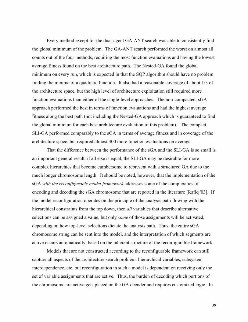
Figures 2.8-2.11 provide a visual representation of search coverage and the resources
spent seeking optimal architectures. Each line on the figure represents an architecture with
the minimum fitness found for that architecture plotted on the vertical axis and the percentage
of function evaluations spent on that architecture plotted on the horizontal axis. The two
dual-level approaches apportion more equal fractions of computation resources to all
architectures, noted in the smaller degree of spread of the lines: most architectures get
between 1 and 5 percent of evaluation resources. With these two, the best architecture (the
line that goes up to 1.0), is not necessarily the one that receives the most function calls. With
the two single-level approaches, the convergence to a best path can be seen in the
apportioning of the most function calls to it. A large percentage of calls is spent on only a
few architectures, while the rest get between .1 and 2 percent of all evaluations. This may
indicate the algorithm is spending a larger percentage of resources trying to improve one or a
few architectures. While it is not as visible in the scaling of the plot axes, for each method
there are many architectures that only receive a small percentage of the total calls: these lines
are all clustered against the y-axis.
The tension between exploration and exploitation is better portrayed in Figure 2.7.
For each run of the algorithms, the number of calls to each explored architecture is averaged.
This serves as an indication of the computing resources that are spent exploiting architectures.
This is compared with the quantity of architectures explored by each algorithm as a
percentage of the total possible architectures in the system. With this representation, it is
clear that the dual-level methods achieve a higher degree of exploitation, spending more calls
for every architecture than do the single-level approaches. The single-level methods have a
low degree of exploitation, but a higher degree of exploration. In balancing these two
objectives, it appears that the GA-ANT method would be a good selection. However, the
performance of the GA-ANT approach is the poorest of the four methods, shown in Table 2.4.
Both single-level approaches achieve larger levels of exploration and on average still identify
all of the top 8 of architectures, indicating adequate exploitation.
35
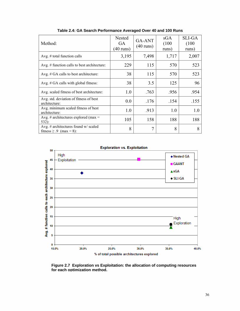
Table 2.4: GA Search Performance Averaged Over 40 and 100 Runs
Method: Nested
GA (40 runs)
GA-ANT (40 runs)
sGA (100 runs)
SLI-GA (100 runs)
Avg. # total function calls 3,195 7,498 1,717 2,007
Avg. # function calls to best architecture: 229 115 570 523
Avg. # GA calls to best architecture: 38 115 570 523
Avg. # GA calls with global fitness: 38 3.5 125 96
Avg. scaled fitness of best architecture: 1.0 .763 .956 .954Avg. std. deviation of fitness of best architecture: 0.0 .176 .154 .155Avg. minimum scaled fitness of best architecture: 1.0 .913 1.0 1.0Avg. # architectures explored (max = 532): 105 158 188 188Avg. # architectures found w/ scaled fitness ≥ .9 (max = 8): 8 7 8 8
Figure 2.7 Exploration vs Exploitation: the allocation of computing resources for each optimization method.
36
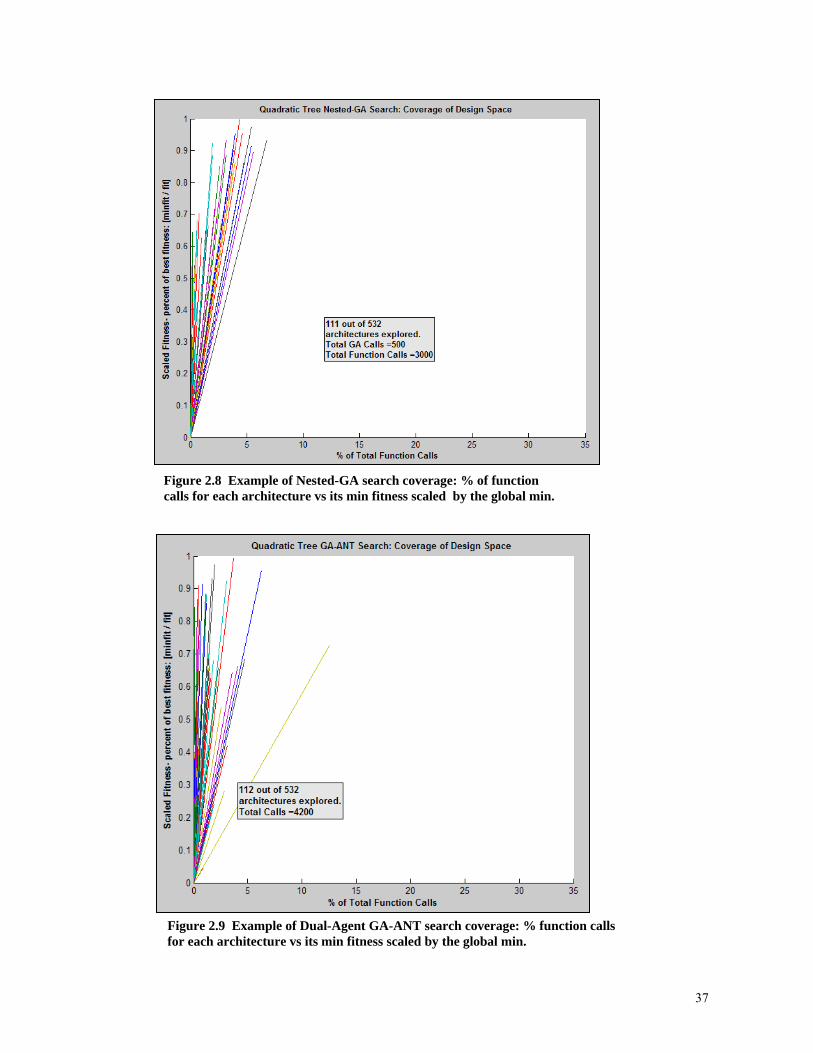
Figure 2.8 Example of Nested-GA search coverage: % of function calls for each architecture vs its min fitness scaled by the global min.
GA-ANT search coverage: % function calls for each architecture vs its min fitness scaled by the global min. Figure 2.9 Example of Dual-Agent
37
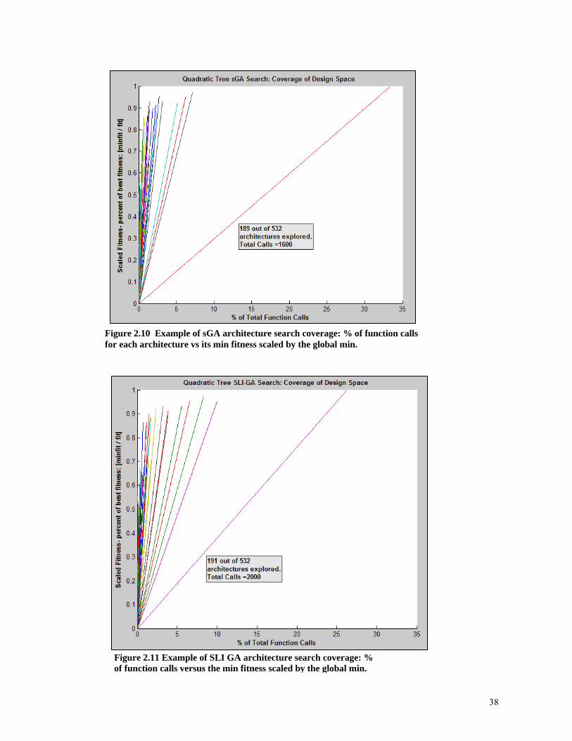
Figure 2.10 Example of sGA architecture search coverage: % of function calls for
Fo
each architecture vs its min fitness scaled by the global min.
igure 2.11 Example of SLI GA architecture search coverage: % f function calls versus the min fitness scaled by the global min.
38
39
ost all
mini
ore
acted, sGA
e of the
d the SLI-GA is so small is
an important general result: if all else is equal, the SLI-GA may be desirable for more
com
entation of the
sGA
03]. If
the m
chrom ents are
activ ework.
ework can still
the c res customized logic. In
Every method except for the dual-agent GA-ANT search was able to consistently find
the global minimum of the problem. The GA-ANT search performed the worst on alm
counts out of the four methods, requiring the most function evaluations and having the lowest
average fitness found on the best architecture path. The Nested-GA found the global
mum on every run, which is expected in that the SQP algorithm should have no problem
finding the minima of a quadratic function. It also had a reasonable coverage of about 1/5 of
the architecture space, but the high level of architecture exploitation still required m
function evaluations than either of the single-level approaches. The non-comp
approach performed the best in terms of function evaluations and had the highest average
fitness along the best path (not including the Nested-GA approach which is guaranteed to find
the global minimum for each best architecture evaluation of this problem). The compact
SLI-GA performed comparably to the sGA in terms of average fitness and in coverag
architecture space, but required almost 300 more function evaluations on average.
That the difference between the performance of the sGA an
plex hierarchies that become cumbersome to represent with a structured GA due to the
much longer chromosome length. It should be noted, however, that the implem
with the reconfigurable model framework addresses some of the complexities of
encoding and decoding the sGA chromosome that are reported in the literature [Rafiq '
odel reconfiguration operates on the principle of the analysis path flowing with the
hierarchical constraints from the top down, then all variables that describe alternative
selections can be assigned a value, but only some of those assignments will be activated,
depending on how top-level selections dictate the analysis path. Thus, the entire sGA
osome string can be sent into the model, and the interpretation of which segm
e occurs automatically, based on the inherent structure of the reconfigurable fram
Models that are not constructed according to the reconfigurable fram
capture all aspects of the architecture search problem: hierarchical variables, subsystem
interdependence, etc, but reconfiguration in such a model is dependent on receiving only the
set of variable assignments that are active. Thus, the burden of decoding which portions of
hromosome are active gets placed on the GA decoder and requi
39
this case, the logic needed to decode the SLI-GA is simpler than that of the sGA because the
sGA st
lligent
rld
ring is based on every selection variable in the model. When hundreds of variables are
included, this essentially leads to hundreds of “if then” statements in the decoder. The SLI-
GA implementation for both the Quadratic Tree problem and the ISRU case study uses
custom logic for decoding because the genes can have multiple expressions: more inte
interpretation is required. With the reconfigurable model framework a generalized, flexible
decoder similar to the sGA is possible, but requires development that was not pursued to
completion in this work.
From the results of the Quadratic Tree architecture search, the single-level search
methods seem to perform the best. The Nested-GA approach provides high-confidence
results, but this is tempered by the simplicity of the continuous design space in the Quadratic
Tree. These approaches will be considered and further assessed in the context of a real-wo
case study, ISRU lunar oxygen production.
40
Chapter 3: ISRU Lunar Oxygen Production
3.1 ISRU Oxygen Production Processes
As NASA prepares for a return to the Moon, an opportunity is unfolding to extend the
in
e
ustainable exploration, higher scientific returns,
lower mission costs. The concept of In-Situ Resource Utilization (ISRU) is simply using
sources that can be found at a present location. Because of NASA’s lunar plans, lunar-
erived resources have the most relevant interest in the short to medium term (2010-2030).
Studies of ISRU and its mission benefits have been performed for decades, but until
cently, most work has been confined to paper studies and a few bench-test experiments of
dividual ISRU components, such as chemical reactors, electrolyzers, or cryocoolers
anders '00]. The Eagle Engineering report of 1988 [Eagle Engineering '88] is one of the
ost comprehensive studies performed, reviewing thirteen chemical processes for lunar
xygen production and developing conceptual designs of pilot oxygen production plants.
hey focused on very large production rates (144-1500 Mt O2/yr) that would support oxygen
se as spacecraft propellant oxidizer. Other ISRU modeling to date has incorporated
reviously reported data and analyses of ISRU chemical processes with economic models to
rovide a higher-level ISRU scenario analysis tool [Belachgar '06].
NASA’s current ISRU program is developing test versions of several different types
f oxygen production systems [Sanders '00]. In conjunction with the hardware development,
ASA has generated a set of detailed engineering models of the major subsystems and
omponents that comprise oxygen production plants [Steffen '07]. Because the technology is
ill in the development stage, the goal of the modeling effort is to answer questions about the
frontier of space exploration beyond the quick forays of the past and create a new paradigm
our approach to space mission planning. Almost every aspect of space mission sustenanc
relies entirely upon materials and supplies carried from Earth including propellants,
pressurants, crew consumables, and tools. Shifting this Earth-based dependence to consider
utilizing in-situ resources may enable more s
and
re
d
re
in
[S
m
o
T
u
p
p
o
N
c
st
41

trade-offs between different technology approaches and the scalability of the systems. Initial
nalyses are assessing production levels in the range of .5 metric tons to 10,000 metric tons
of oxygen per year—quantities that would be applicable to crew air supply [Chepko '08].
living
n the lunar surface for one year. The analysis, performed using a space logistics planning
and simulation tool called SpaceNet, assumes a 90% environmental life-support system
s (extra-vehicular activities: spacewalks)
a
Table 3.1 provides an example breakdown of the oxygen needs for a four-person crew
o
closure and an average of five, eight-hour long EVA’
performed per week [de Weck O.L. '07; Armar '08].
Table 3.1: Lunar Base Crew Oxygen Consumption
Oxygen Usage Quantity Consumed [kg/yr]
Habitat (90% ECLSS closure) 1132.7
Leakage and Venting 6.2
EVA O2 373.4
EVA airlock 34.4
Total: 1546.7
Lunar oxygen extraction can be accomplished via several different chemical
processes. Three of these are receiving primary focus for development: hydrogen reduction
carbothermal reduction, and electrowinning. Of these three, only hydrogen and carbother
reduction have currently been modeled sufficiently to incorporate into an ISRU system
architecture search. An oxygen plant system design consists of a reactor that uses one of
these chemical processes and the supporting hardware necessary to operate the reactor
condition the reaction products such that the result is stored liquid oxygen of a specified
purity.
,
mal
and
42

3.1.1 Hydrogen Reduction
Lunar regolith is comprised of about 42% oxygen by mass that exists in the form of
glasses (mostly SiO
e
s of
orm water. Water vapor is removed
from the reactor and electrolyzed to form oxygen that is sent to storage and hydrogen that is
recycled to the reactor. ture reaction
chambers, a hy system, water se s, along with
mechanisms to system and the separate gas streams. A
schematic of hydrogen reduction is shown in Figure 3.1.
Hydrogen Reduction: FeO.TiO2(s) + H2(g ) → Fe(s ) + TiO2(s) + H2O
Electrol 2O(g) + electricity → H2(g) + 1/2 O2(g) (3.2)
2) and metal oxides. The hydrogen reduction processes targets the iron
oxide (FeO) in the glasses and metal oxides such as ilmenite, FeOTiO2, (Eqn. 3.1-3.2) [Hegd
'08]. Hydrogen reduction is a reaction capable of extracting between 1% and 5% by mas
oxygen-to-regolith. Regolith is heated to between 700°C and 1000°C and exposed to
hydrogen that reacts with weakly bonded oxygen to f
Hydrogen reduction systems require high-tempera
drogen gas flow paration and electrolysis system
handle regolith into and out of the
(g ) (3.1)
ysis: H
Regolith Feed
ReactorSeparation
& Electrolysis
Liquefaction & Storage
H2 Feed & Supply
H2 + H2O
fresh regolith
H2
O2
H2
spent regolith
H2 Recycling System
Regolith Feed
ReactorSeparation
& Electrolysis
Liquefaction & Storage
H2 Feed & Supply
H2 + H2O
fresh regolith
H2
O2
H2
spent regolith
H2 Recycling System
Figure 3.1 Hydrogen reduction schematic.
43
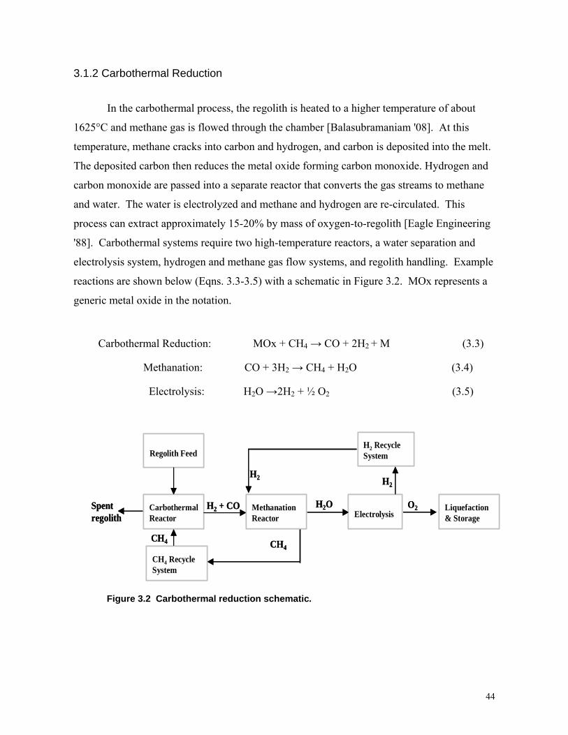
3.1.2 Carbothermal Reduction
thane
d
a
Carbothermal Reduction: MOx + CH → CO + 2H + M (3.3)
Methanation: CO + 3H2 → CH4 + H2O (3.4)
Electrolysis: H2O →2H2 + ½ O2 (3.5)
In the carbothermal process, the regolith is heated to a higher temperature of about
1625°C and methane gas is flowed through the chamber [Balasubramaniam '08]. At this
temperature, methane cracks into carbon and hydrogen, and carbon is deposited into the melt.
The deposited carbon then reduces the metal oxide forming carbon monoxide. Hydrogen and
carbon monoxide are passed into a separate reactor that converts the gas streams to me
and water. The water is electrolyzed and methane and hydrogen are re-circulated. This
process can extract approximately 15-20% by mass of oxygen-to-regolith [Eagle Engineering
'88]. Carbothermal systems require two high-temperature reactors, a water separation an
electrolysis system, hydrogen and methane gas flow systems, and regolith handling. Example
reactions are shown below (Eqns. 3.3-3.5) with a schematic in Figure 3.2. MOx represents
generic metal oxide in the notation.
4 2
CarbothermalReactor
Regolith Feed
MethanationReactor Electrolysis
Liquefaction & Storage
CH4 Recycle System
H2 Recycle System
H2 + CO H2O
CH4CH4
H2H2
O2Spent regolith
CarbothermalReactorCarbothermalReactor
Regolith FeedRegolith Feed
MethanationReactorMethanationReactor ElectrolysisElectrolysis
Liquefaction & StorageLiquefaction & Storage
CH4 Recycle SystemCH4 Recycle System
H2 Recycle SystemH2 Recycle System
H2 + CO H2O
CH4CH4
H2H2
O2Spent regolith
Figure 3.2 Carbothermal reduction schematic.
44
3.1.3 Molten Salt Electrolysis (Electrowinning)
olten Salt Electrolysis: Fe2+ + 2e- → Fe , Si4+ + 4e- → Si Cathode (3.6)
The key challenge in selecting a particular process for lunar oxygen production is that
the processes with higher yields of oxygen are also more complex and power intensive. The
basic question then is what is better: low-yield plants with less complexity, or high-yield
plants with higher complexity? The baseline oxygen plant design is for the above processes
to occur in batch fashion, i.e. discrete quantities of fresh regolith are deposited to and
removed from the reactor, rather than allowing for continuous flow of regolith and reactants.
Aside from reaction efficiency, the overall production rate of liquid oxygen depends mainly
on the number of reactors, the size of each reactor, and the speed of reaction. Speed of
reaction is affected by the time required to bring regolith batches up to reaction temperatures
and have different power requirements: a
larger reactor requires a more thermal energy to raise regolith from lunar ambient
temperatures of ~300K to reaction temperatures. The current designs plan on solar
Electrowinning differs from the previous two methods. This is an electrochemical
reaction generally used to extract metals from their ores. The regolith metal oxides are
immersed in a liquid electrolyte or liquefied with a molten salt and used as the cathode. Upon
application of electricity, oxygen is evolved at the anode. This process requires higher
temperatures to fully melt the regolith, but extracts almost all of the oxygen in the regolith—
42%. The technique is less developed than other methods, with challenges to be met in
increasing the reaction rates, but offers the potential of a higher yield. Electrowinning
systems require a high-temperature electrolysis cell, a form of electrolyte, a way to capture
slag and clear electrodes for new batches, and regolith and oxygen handling mechanisms. An
example reaction using molten salt is shown below.
M
4(SiO-) = 2(Si-O-Si) + O2 + 4e- Anode (3.7)
3.2 ISRU Architecture Trade Space
by the reactant gas flow rates. These factors each
45
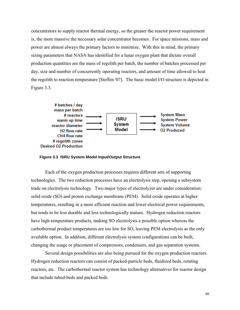
concentrators to supply reactor thermal energy, so the greater the reactor power requirement
, the m nd
y
d per
ted in
Each of the oxygen production processes requires different sets of supporting
technol
ors
.
tating
r design
that include tubed-beds and packed beds.
is ore massive the necessary solar concentrator becomes. For space missions, mass a
power are almost always the primary factors to minimize. With this in mind, the primar
sizing parameters that NASA has identified for a lunar oxygen plant that dictate overall
production quantities are the mass of regolith per batch, the number of batches processe
day, size and number of concurrently operating reactors, and amount of time allowed to heat
the regolith to reaction temperature [Steffen '07]. The basic model I/O structure is depic
Figure 3.3.
ogies. The two reduction processes have an electrolysis step, opening a subsystem
trade on electrolysis technology. Two major types of electrolyzer are under consideration:
solid oxide (SO) and proton exchange membrane (PEM). Solid oxide operates at higher
temperatures, resulting in a more efficient reaction and lower electrical power requirements,
but tends to be less durable and less technologically mature. Hydrogen reduction react
have high-temperature products, making SO electrolysis a possible option whereas the
carbothermal product temperatures are too low for SO, leaving PEM electrolysis as the only
available option. In addition, different electrolysis system configurations can be built,
changing the usage or placement of compressors, condensers, and gas separation systems.
Several design possibilities are also being pursued for the oxygen production reactors
Hydrogen reduction reactors can consist of packed-particle beds, fluidized beds, ro
reactors, etc. The carbothermal reactor system has technology alternatives for reacto
Figure 3.3 ISRU System Model Input/Output Structure
46
NASA’s growing library of analysis models capture many of these subsystem and
component options, even including options for insulation and construction materials. These
models are connected together in various combinations to form NASA’s ISRU System Mo
for a steady-state, system-level analysis [Sanders '00; Steffen '07]. In the current version
the ISRU System Model, each of the major architectures is constructed in a standalone,
separate piece of software. These include hydrogen reduction with SO electrolyzer, hydrogen
reduction with PEM electrolyzer, and carbothermal reduction with PEM electrolyzer. A
molten salt e
del
of
lectrolysis model is under development. Trade studies and architecture
comparisons are assessed on a point-to-point basis via manual exploration of the architecture
variables between the several system model versions. Component model updates require
editing of complex system model files, and incorporation of new oxygen production processes
require construction of a new standalone system model version.
Because the ISRU program is considering a large, hierarchical architecture space of a
complex system that incorporates developing technologies, it is an ideal case study for the
flexible modeling framework and architecture search tools developed in Chapter 2. By
applying the modeling framework to the existing ISRU System Model, issues with model
updates and architecture additions can be addressed, and a deeper understanding and wider
search of the architecture possibilities can be explored [Chepko '08].
47
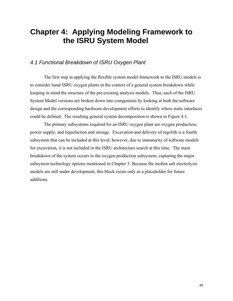
Chapter 4: Applying Modeling Framework to the ISRU System Model
4.1 Functional Breakdown of ISRU Oxygen Plant
The first step in applying the flexible system model framework to the ISRU mode
to consider lunar ISRU oxygen plants in the context of a general system breakdown w
keeping in mind the structure of the pre-existing analysis models. Thus, each of the ISRU
System Model versions are broken down into components by looking at both the software
design and the corresponding hardware development efforts to identify where static interfaces
could be defined. The resulting general system decomposition is s
ls is
hile
hown in Figure 4.1.
els
lten salt electrolysis
odels are still under development, this block exists only as a placeholder for future
dditions.
The primary subsystems required for an ISRU oxygen plant are oxygen production,
power supply, and liquefaction and storage. Excavation and delivery of regolith is a fourth
subsystem that can be included at this level; however, due to immaturity of software mod
for excavation, it is not included in the ISRU architecture search at this time. The main
breakdown of the system occurs in the oxygen production subsystem, capturing the major
subsystem technology options mentioned in Chapter 3. Because the mo
m
a
48
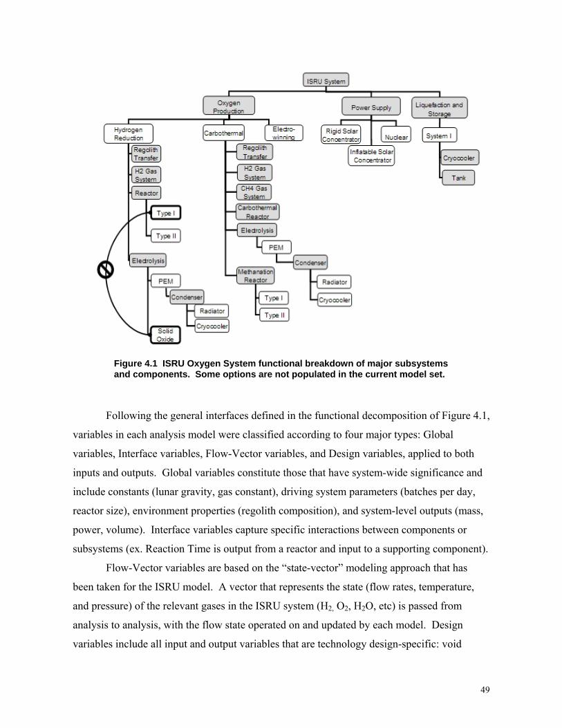
Following the general interfaces defined in the functional decomposition of Fi
variables in e
gure 4.1,
ach analysis model were classified according to four major types: Global
variables, Interface variables, Flow-Vector variables, and Design variables, applied to both
inputs and outputs. Global variables constitute those that have system-wide significance and
include constants (lunar gravity, gas constant), driving system parameters (batches per day,
reactor size), environment properties (regolith composition), and system-level outputs (mass,
power, volume). Interface variables capture specific interactions between components or
subsystems (ex. Reaction Time is output from a reactor and input to a supporting component).
Flow-Vector variables are based on the “state-vector” modeling approach that has
been taken for the ISRU model. A vector that represents the state (flow rates, temperature,
and pressure) of the relevant gases in the ISRU system (H2, O2, H2O, etc) is passed from
analysis to analysis, with the flow state operated on and updated by each model. Design
variables include all input and output variables that are technology design-specific: void
Figure 4.1 ISRU Oxygen System functional breakdown of major subsystems and components. Some options are not populated in the current model set.
49

fraction of a packed-bed reactor, calculated thickness of insulation, etc. These are the
variables that are unique to each analysis model that effect or describe the specific design.
These four classifications help the modelers to identify the stable interface points
between modules and organize the vast number of variables into a structure that is easier to
navigate and peruse. In addition, grouping the interface variables together provides a flag
point for an automated software tool to identify the correct variables to link into the analysis
path. The software does not need to “know” what every variable in every analysis module is:
it can simply look for the group classified as “Interface” and pass whatever is contained in the
group to the rest of the system model.
4.2 Implementation of ISRU System Architecture model
The new structure for the ISRU System Architecture Model is implemented using
Phoenix Integration’s ModelCenter, a tool that enables data flow between separate models.
ModelCenter has a graphical interface that shows variable linkages and allows control and
execution of all models tied into the environment. The ISRU System Model is built following
the system decomposition with model repositories at each “OR” level in the structure. The
existing Excel-based subsystem and component models are used to populate the structure and
define subsystem interactions. A linking tool was created to enable simple, programmatic re-
linking betw
e
een “OR” level options based on values assigned to a set of “option” variables.
When selected, a particular “OR” level model is tied in to the system model by finding its
Global, Interface, and Flow-Vector variables and linking them to the “placeholder” modules
that contain the relevant variable interfaces. The placeholders help create a break-point where
the analysis path can be switched from one model to another. Figure 4.2 and 4.3 illustrate th
implementation of the ISRU System Model.
50
Figure 4.2. ModelCenter: top level of model showing O2 production, Power, and Liquefacsubsystems. Connecting lines represent data flow of subsystem interdependence. An exploretree on the left displays all variables and their values, and allows manual changes to input variables.
tion r
Figure 4.3. ModelCenter: “OR” Level model repository of O2 Production Options. Only one option is tied into analysis path (represented by the connecting arrows) at a time. “Input” and “Output” modules are the placeholders defining the stable interfaces.
51
52 52
With the stable interfaces and repository points, the ISRU System Model can be
expanded to include future options or updated with newer versions of existing models by
simply loading the new model into the proper repository. If the interface variables have been
defined correctly, automatic linking into the system can be accomplished. Thus, in a
simplified explanation, any oxygen production process can be added as long as it operates on
a quantity of regolith and outputs a quantity of oxygen. Similarly, at a lower level, any
hydrogen reduction reactor can be included in the system as long as it receives a quantity of
regolith and hydrogen and outputs a quantity of water vapor. These basic functional
definitions serve as the static model framework. Additional detailed and model-specific
inputs can be changed throughout the model, but preserving the static interfaces enables a
flexible, reconfigurable system model.
4.3 Application of Architecture Optimization
ap r
system-level trade-offs and impacts were selected to define the architecture space. At this
stage of model development, the primary technology choices lie within the oxygen production
subsystem. Several of the existing components and subsystems do not have more than one
technology option represented in the model (ex. the regolith transfer component and gas feed
systems each have only one option in their repository). Thus the tree in Figure 4.4 represents
only the current discrete variable space that is included in the architecture optimization
problem. There are 522 possible architecture combinations, accounting for the single
compatibility constraint between hydrogen reduction reactors that cool exit gases and the
high-temperature SO electrolyzer.
With the reconfigurable structure in place, architecture optimization tools can be
plied the ISRU System Model. The technology variables that exhibit the most potential fo
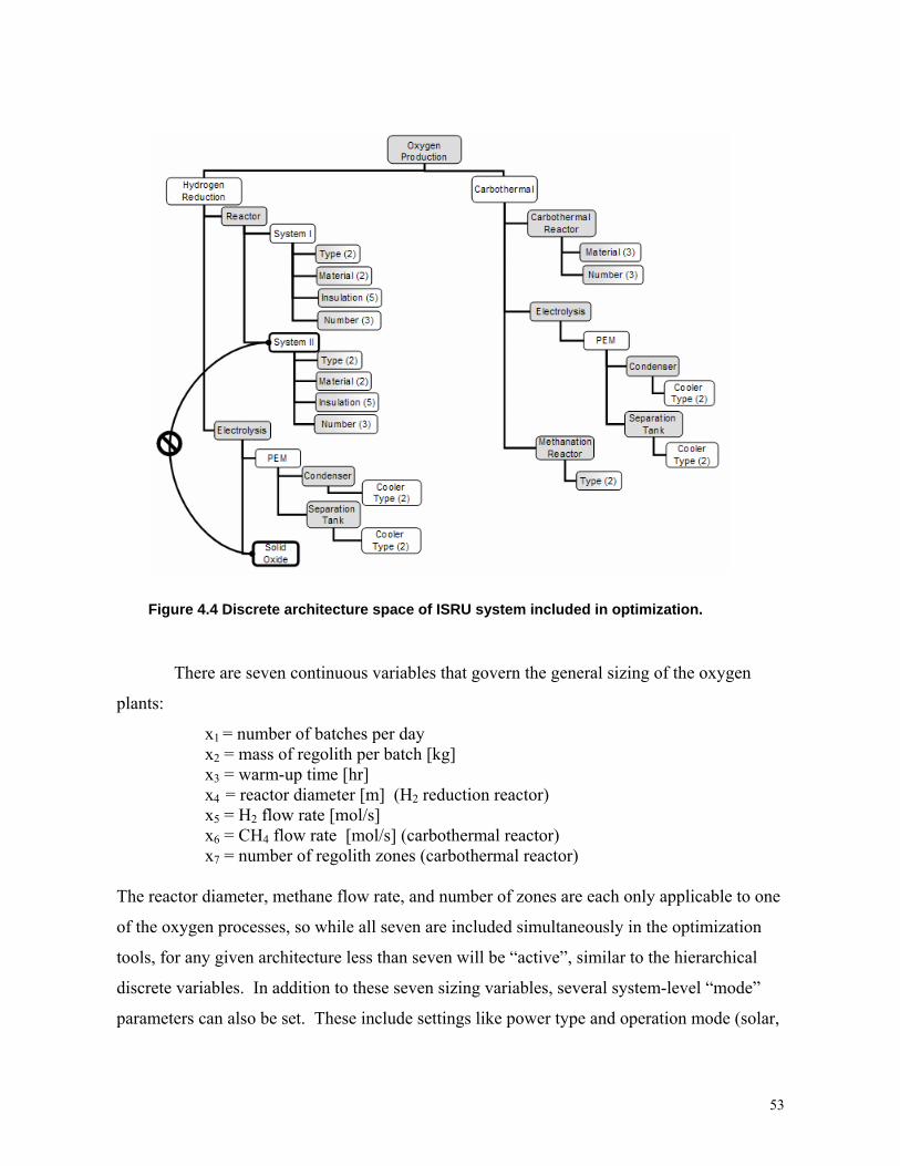
There are seven continuous variables that govern the general sizing of the oxygen
plants:
x1 = number of batches per day x2 = mass of regolith per batch [kg] x3 = warm-up time [hr] x4 = reactor diameter [m] (H2 reduction reactor) x5 = H2 flow rate [mol/s] x6 = CH4 flow rate [mol/s] (carbotherm x
al reactor) zones (carbothermal reactor)
The reactor diameter, methane flow rate, and number of zones are each only applicable to one
of the oxygen processes, so while all seven are included simultaneously in the optimization
tools, for any given architecture less than seven will be “active”, similar to the hierarchical
discrete variables. In addition to these seven sizing variables, several system-level “mode”
parameters can also be set. These include settings like power type and operation mode (solar,
7 = number of regolith
Figure 4.4 Discrete architecture space of ISRU system included in optimization.
53

radioisotope generators, etc); the location of the power system (dictates the amount of time
force
ters.
per lunar day that solar power is available); and desired annual oxygen production rate.
For the purposes of this case study, all optimization runs are based on a system using
only solar power and located near the Shackleton Rim, which has shorter lunar nights. A
range of oxygen production rates are analyzed to determine if the high-performing
architectures for low production rates are the same configurations as for high production rates.
To evaluate a particular architecture, the model is linked according to the discrete variable
settings and executed with the values set for the continuous parameters. The resulting outputs
indicate the achievable quantity of oxygen produced per year (based on input batch rate, size,
and reaction rates), a system mass, and power usage. For all optimization methods, the
objective is to minimize system mass subject to a few constraints. These constraints en
the production rate to within a small range of the input desired rate and ensure feasibility of
timing (the end-to-end, calculated batch processing time must be less than the time dictated by
the input batches per day). In addition, bounds are placed on the continuous input parame
Equations 4.1-4.3 present the mathematical formulation of the constraints.
0O -1 g 21 ≤=
produced
O2desired (4.1)
( ) 01____
2 ≤−24
++=
transferregolithTimewarmupTimereactionTimeg (4.2) hPerDayNumberBatc
x iiLB xxiub≤≤ (4.3)
Ad tm aneous processing when multiple reactors are
be g u
4.3 1 F
e
minimum, attempts made using different initial points resulted in different convergence
jus ents are made to g2 to account for simult
in sed.
. ull Enumeration Attempts
The same enumeration scheme used on the Quadratic Tree problem was applied
to the ISRU system using ModelCenter’s built-in SQP optimizer. Problems arose, however,
in that the continuous design space of the ISRU system is more complex than the simple
quadratics assessed earlier, and the optimizer often had difficulties finding minima, or in som
cases even feasible solutions. Even for the architectures that the SQP converged on a
54
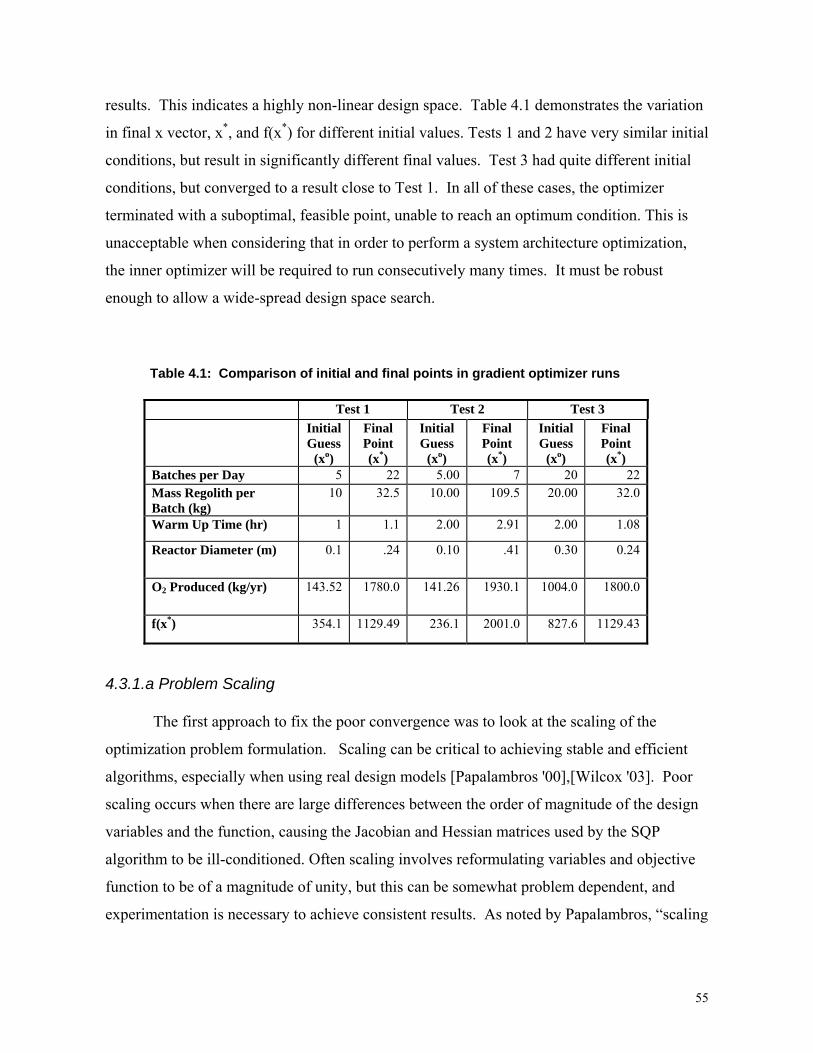
results. This indicates a highly non-linear design space. Table 4.1 demonstrates the variatio
in final x vector, x
n
nitial
conditi
This is
*, and f(x*) for different initial values. Tests 1 and 2 have very similar i
ons, but result in significantly different final values. Test 3 had quite different initial
conditions, but converged to a result close to Test 1. In all of these cases, the optimizer
terminated with a suboptimal, feasible point, unable to reach an optimum condition.
unacceptable when considering that in order to perform a system architecture optimization,
the inner optimizer will be required to run consecutively many times. It must be robust
enough to allow a wide-spread design space search.
Table 4.1: Comparison of initial and final points in gradient optimizer runs
Test 1 Test 2 Test 3 Initial
Guess (xo)
Final Point (x*)
Initial Guess
(xo)
Final Point (x*)
Initial Guess
(xo)
Final Point (x*)
Batches per Day 5 22 5.00 7 20 22 Mass Regolith per 10 32.5 10.00 109.5 20.00 Batch (kg)
32.0
Warm Up Time (hr) 1 1.1 2.00 2.91 2.00 1.08
Reactor Diameter (m) 0.30 4 0.1 .24 0.10 .41 0.2
O2 Produced (kg/yr) 143.52 1780.0 141.26 1930.1 1004.0 1800.0
f(x*) 354.1 1129.49 236.1 2001.0 827.6 1129.43
rst approach to fix the poor convergence was to look at the scaling of the
caling can be critical to achieving stable and efficient
lgorithms, especially when using real design models [Papalambros '00],[Wilcox '03]. Poor
scaling sign
ive
scaling
4.3.1.a Problem Scaling
The fi
optimization problem formulation. S
a
occurs when there are large differences between the order of magnitude of the de
variables and the function, causing the Jacobian and Hessian matrices used by the SQP
algorithm to be ill-conditioned. Often scaling involves reformulating variables and object
function to be of a magnitude of unity, but this can be somewhat problem dependent, and
experimentation is necessary to achieve consistent results. As noted by Papalambros, “
55
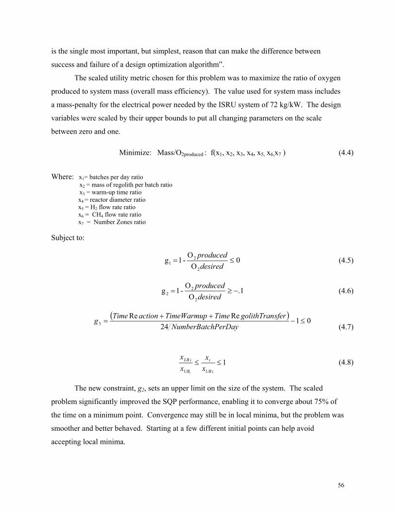
is the single most important, but simplest, reason that can make the difference between
success and failure of a design optimization algorithm”.
The scaled utility metric chosen for this problem was to maximize the ratio of oxygen
produced to system mass (overall mass efficiency). The value used for system mass incl
a mass-penalty for the electrical power needed by the ISRU system of 72 kg/kW. The design
variables were scaled by their upper bounds to put all changing parameters on the scale
between zero and one.
udes
Minimize: Mass/O2produced : f(x1, x2, x3, x4, x5, x6,x7 ) (4.4)
Where:
x3 = warm-up time ratio
x4 = reactor diameter ratio 5 = H2 flow rate ratio x6 = CH4 flow rate ratio x7 = Number Zones ratio
Subjec
x1= batches per day ratio x2 = mass of regolith per batch ratio
x
t to:
0O
O2 -1 2
1 ≤=des
produced
gired
(4.5)
1. (4.6) O
2 −≥=desiredro
( )
O-1 2 pg2
duced
01243 ≤−
ReRe ++=
hPerDayNumberBatcg sfergolithTranTimeTimeWarmupactionTime
(4.7)
1≤≤iUB
i
UB
iLB
xx
xx
i
The new constraint, g
(4.8)
of
s
2, sets an upper limit on the size of the system. The scaled
problem significantly improved the SQP performance, enabling it to converge about 75%
the time on a minimum point. Convergence may still be in local minima, but the problem wa
smoother and better behaved. Starting at a few different initial points can help avoid
accepting local minima.
56
4.3.1.b Simulated Annealing To improve confidence in the SQP results and aim for a global minimum, for each
architec
search, but instead use probabilistic operators that direct a random
arch through the de
of molecular energy states as hot metal cools and freezes to a minimum-energy crystalline
n, a perturbing function changes the design variables,
and the subsequent function evaluation is accepted if it is better than the last. If the objective
va ious objective, it may still be accepted with some probability,
based on a “temperature” value. This probability decreases as the algorithm progresses,
perature cooling in the metal annealing process. Simulated annealing is a
owerful tool to apply to highly non-linear systems because i
local minima.
A MATLAB-based simulated annealing algorithm was modified for the ISRU
. Constraints were handled using a quadratic exterior pe
objective function will have a penalty added to it when constraints are violated. The
agnitude of the penalty changes with the square of the constraint violation. Simul
annealing is computationally expensive and can take hundreds to thousands of function
evaluations to converge on a global optimum. For the ISRU System Model, to balance
etween time and fidelity of the results, an additional ter
search after 100 evaluations without finding a new, better point. This will usually result in
termina
.
00-300
n evaluation took around 10 seconds, depending on the system
architecture configuration. Because of the computational time required for simulated
ture the SQP algorithm was run three times from different initial points. For the
instances when SQP still could not find a minimum at all, a tool was created to switch the
problem to use a heuristic technique, simulated annealing (SA), to search the continuous
space. Heuristic search algorithms such as simulated annealing do not use gradient
information to guide the
se sign space. Simulated annealing is a process modeled after the behavior
state [Kirkpatrick '83].
A random starting point is chose
lue is not better than the prev
mimicking the tem
p t can overcome being trapped in
problem nalty method, thus the
m ated
b mination criteria was set to end the
tion without an optimum design, but it still provides a good answer for system
comparisons and can be used as a starting point for finer-tuned further optimization if needed
From trial runs with varying architecture options, simulated annealing took between
200 and 700 iterations to terminate, compared to SQP which was generally between 1
evaluations. Each functio
57
annealing, it was only used in the ISRU System Model optimization tool after two or more
itial s
an
ility
erate the ISRU architecture space required at least 1566 separate
ptimiz
es are based on a single 3.0 GHz processor. Clearly, this is unreasonable for
an arly as
r for
A
less
still lon
in tarting points with the SQP gradient method failed. If a feasible point could not be
found, the optimization tool switched to simulated annealing. A drawback to simulated
annealing aside from computation time is that constraint handling via the penalty method c
still result in infeasible designs. Simulated annealing results need to be checked for feasib
after termination.
4.3.1.c The Cost of Full Enumeration
Because the SQP-SA optimization tool required at least three optimization runs per
architecture, to fully enum
o ation runs. Even if each run averaged needing only 200 function evaluations to
converge, this amounts to 313,200 function evaluations needed to fully enumerate the
architecture space within internal optimization. This would require about 30 days to
accomplish with the current runtimes seen with the ISRU System Model. Even if the
confidence factor of executing each architecture from three different initial points was
reduced to one, full enumeration would still take on the order of 10 days to complete. These
computation tim
e -stage design study. With this realization, attempts at full enumeration as well
application of the Nested-GA approach were abandoned. Executing a gradient optimize
every architecture evaluation is too computationally expensive. However, the SQP-S
method can be reserved for “fine tuning” of designs that have been identified by other means.
4.3.2 Genetic Algorithm Methods
With enumeration and the Nested-GA ruled out, the sGA, SLI-GA, and GA-ANT
approaches were applied to the ISRU System Model. Limiting population size to be either
100 or 70 and using a maximum generation limit of 80 reduces the possible runtimes to
than two days. Most runs ended up requiring between 8 and 12 hours to converge, which is
g, but at least within the realm of feasibility to generate useful results.
58

Table 4.2: Computation Time Comparison Optimization Method Estimated Run Time
Full Enumeration 10 - 30 days
Nested GA ~10 days
sGA, SLI-GA, GA-ANT 8 – 12 hrs
4.3.2.a Chromosome Representations
ion did not change much from the Quadratic Tree,
s the architecture sizes were about the same in each problem. 16 variable genes were needed
d 8
256 8256 8
80
Carb. Reac. Material
H2 Red. PEM Condenserk
CH4 Flow Rate# Regolith Zones
Con
t
Total Chromosome Length:
The sGA chromosome representat
a
for the discrete space of the structured GA. With the 7 continuous variables, the real-valued
chromosome length was 23 genes. Continuous variables were discretized with resolutions
ranging from .004 to .01 (all variables were scaled to be between 0 and 1), which require
bits and 256 choices for each. Table 4.3 shows the sGA chromosome.
Table 4.3: sGA Chromosome for ISRU Architecture # choices # Bits
2 12 12 13 42 12 15 32 12 15 3
Gene:O2 OptionH2_Red. Reactor SystemH2 Red Elec. Type # ReactorsH2_Red Reac. 1, MaterialH2_Red. Reac. 1, Reactor TypeH2_Red. Reac. 1, InsulationH2_Red. Reac. 2, MaterialH2_Red. Reac. 2, Reactor TypeH2_Red. Reac. 2, Insulation
Subs
yste
m I
2 12 13 22 12 12 1
256 8256 8256 8256 8256 8
Carb. Reactor TypeCarb. PEM CondenserCarb. Seperation Tank
inuo
us
Varia
bles
# Batches per DayMass Reg. per BatchWarm Up TimeReactor Diameter
Subs
yste
m
II
H2 Flow Rate
H2 Red PEM Seperation Tan
59

The SLI-GA chrom nes, totaling a full length
of 15 genes, shown in Table 4.4. W representation, the expression of all discrete
genes except the num ent of the O2 Option gene. The
dynamic domain ma discussed in Chapter 2 is used to ensure feasible gene
assignments for all c
Table 4.4: SLI-GA Chromosome for ISRU Architecture Search
256 8256 8256 8256 8
67
Reactor DiameterH2 Flow RateCH4 Flow Rate# Regolith ZonesTotal Chomsome Length
# Batches per Day
osome is reduced to 8 discrete variable ge
ith the SLI
ber of reactors depends on the assignm
pping method
ombinations.
# choices # Bits3 22 12 12 12 15 32 12 1
Electrolysis Condeser TypeElectrolysis Seperation TankReactor Type
Gene:
O2 OptionElectrolysis Type
# Reactors
Reactor InsulationReactor Material
256 8256 8256 8
Mass Reg. per BatchWarm Up Time
4.3.2.b Compatibility Constraints in the ISRU System Model
The single compatibility constraint in the ISRU System Model exists between
assignment of a hydrogen reduction reactor system and the electrolysis option. When PEM
electrolysis is selected, a reactor system must be selected that conditions the high-temperature
products to the low-temperature maximum threshold of the PEM electrolyzer. Conversely,
when the Solid Oxide electrolyzer is chosen, the reactor system accompanying it must output
high-temperature products that are above the SO electrolyzer’s minimum temperature
threshold. This constraint is handled in the chromosome decoding process with the dynamic
domain limiting methods that handle the hierarchical constraints.
For the sGA, in the initial problem set-up, a user defines the compatibility constraint.
This field is checked by the GA during decoding, and when a gene is flagged with a
compatibility constraint, the GA matches the assigned value of the constrained variable with
60
the domain limitations implied by the assignment. Thus, when a H2 Reduction PEM
electrolyzer is selected, the allowed domain of the reactor system is limited to the system
including a heat exchanger that properly conditions the gas stream.
The strength in the sGA implementation of constraint handling is that the logic can
generalized, allowing any new constr
be
aint to be applied based on a user-edited input file. This
eneralization requires some redundancy of variables: “Reactor System” must be included as
a switch variable at include
Material, Insulation, and Reactor Type. The nuance of the sGA decoding implementation
with the reconfigurable model framework is that all discrete variables in the system model are
assigned, passed into the model, and values set. It is the reconfiguration of the model via the
linking tool that controls the analysis path: even though the Carbothermal Reactor Type gene
gets set in the model to “packed-bed”, if the O2 Option gene is set to “H2 Reduction”, when
re-linking occurs, only the H2 Reduction gene assignments have impact on the analysis.
This is different from the SLI-GA decoding implementation. Due to the dual-nature
of the genotype, a “smarter” decoder is required to determine which variables to set in the
model. The burden of controlling the analysis path is placed on the GA’s interpretation of the
genes and not the model’s reconfiguration. This requires more custom logic, but results in
fewer genes in the chromosome. In this case, the compatibility constraints re built into the
logic; through a series of “if-then” statements, the GA checks the O2 Option gene, and
the H2 Reduction path or
the Carbotherm
e
ethods.
g
to properly direct the analysis path for its “child” variables th
a
depending on its value, either interprets the following genes to be in
al path. If H2 Reduction PEM electrolysis is assigned, the compatibility
constraint automatically assigns Reactor System to the heat exchanger version because the
domain is limited to one option. The following Reactor System “child” genes are assigned
accordingly on the heat exchanger analysis path. Because of the custom logic, the Reactor
System variable is unnecessary to include in the chromosome. The strength of this approach
is that is allows an even more compact representation and eliminates duplicate chromosom
strings. The main disadvantage is that it requires custom logic to be built into the decoder.
This may be possible to address with more advanced programming m
61
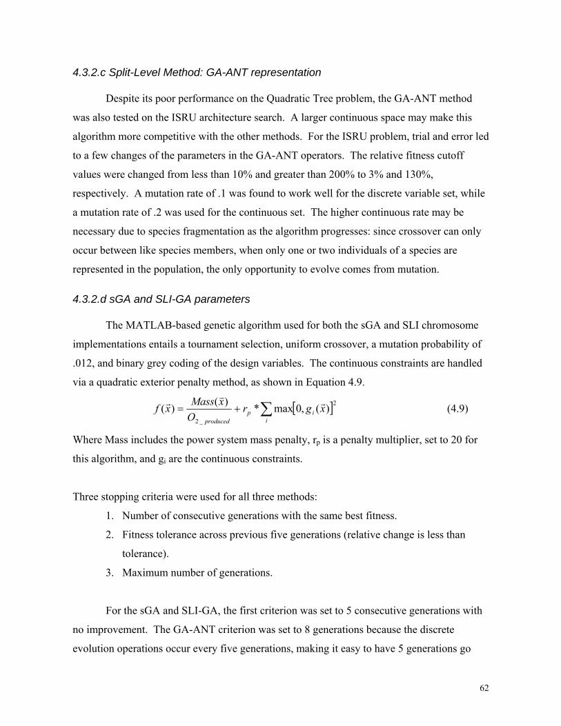
4.3.2.c Split-Level Method: GA-ANT representation
Despite its poor performance on the Quadratic Tree problem, the GA-ANT method
was also tested on the ISRU architecture search. A larger continuous
space may make this
algorith
hile
f
m more competitive with the other methods. For the ISRU problem, trial and error led
to a few changes of the parameters in the GA-ANT operators. The relative fitness cutoff
values were changed from less than 10% and greater than 200% to 3% and 130%,
respectively. A mutation rate of .1 was found to work well for the discrete variable set, w
a mutation rate of .2 was used for the continuous set. The higher continuous rate may be
necessary due to species fragmentation as the algorithm progresses: since crossover can only
occur between like species members, when only one or two individuals of a species are
represented in the population, the only opportunity to evolve comes from mutation.
4.3.2.d sGA and SLI-GA parameters
The MATLAB-based genetic algorithm used for both the sGA and SLI chromosome
implementations entails a tournament selection, uniform crossover, a mutation probability o
.012, and binary grey coding of the design variables. The continuous constraints are handled
via a quadratic exterior penalty method, as shown in Equation 4.9.
[ ]2_2
)(,0max*)()( ∑+=i
ipproduced
xgrO
xMassxf rv
r (4
Where Mass includes the power system mass penalty, r
.9)
or the sGA and SLI-GA, the first criterion was set to 5 consecutive generations with
no improvement. The GA-ANT criterion was set to 8 generations because the discrete
evolution operations occur every five generations, making it easy to have 5 generations go
p is a penalty multiplier, set to 20 for
this algorithm, and gi are the continuous constraints.
Three stopping criteria were used for all three methods:
1. Number of consecutive generations with the same best fitness.
2. Fitness tolerance across previous five generations (relative change is less than
tolerance).
3. Maximum number of generations.
F
62
without overall fitness improvement. The fitness tolerance for sGA and SLI-GA was set to
e-4. T
hown in
Figure 4.5. The key points to note are the multiple sections of “hill-climbing” (these moves to
id becoming trapped in local minima) and the
lower
adient information, there
is no way to guarantee optimality.
ation of the last generation of the run repr ented n Figu e 4.5,
s
s, search is occurring mostly within the
ontinuous variable set. Table 4.5 shows the variance of the last generation: only eight
, and of these, only four variations
among n”, “Electrolyzer
Type”,
all but 1 architecture had settled to “Hydrogen Reduction, SO Electrolyzer, and Loosely-
Packed tors” variable and the lower-level variables
ere the main source of variance in the discrete variable set. This indicates that a faster
architec
1 his criteria was not used for the GA-ANT method. Throughout the trial runs, the
maximum generations ranged from 50 to 80, depending on each algorithms relative speed of
convergence.
4.4 ISRU Architecture Search Results
4.4.1 GA Convergence History
For performance comparison, each of the three GA methods was run four times for an
oxygen plant with a production quantity of 1000 kg/yr. For every run, optimization
terminated on the maximum generation criteria. An example convergence history is s
worse-fitness points enable the GA to avo
s rate of improvement for the later generations. This slower rate can mean either that
the GA has become trapped in a minima without enough diversity in the population to
overcome it, or that it has settled near a global minimum and further progress is only in “fine-
tuning” the continuous values. Because the GA operates without gr
On examin es i r there is
very little variation in the architectures of the population and more variation in the continuou
parameters, so it is assumed that in the later generation
c
distinct architectures were present in the final generation
the primary discrete variables were present. Considering “O2 Optio
“Reactor Type”, and “Number of Reactors” to be the primary architecture variables,
Reactor Type”. The “Number of Reac
w
ture search could be performed by decreasing the maximum generation criteria. Once
the GA converges on one or a few architectures, further optimization of the continuous
63
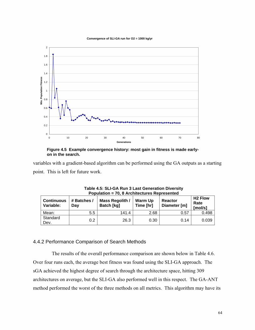
Convergence of SLI-GA run for O2 = 1000 kg/yr
1.8
2
0
0.2
0.4
0.6
0 10 20 30 40 50 60 70 80
Generations
0.8
1.2
1.6
Min
. Po
Fitn
es
1
pula
tion
1.4
s
variables with a gradient-based algorithm can be performed using the GA outputs as a starting
point. This is left for future work.
Table 4.5: SLI-GA Run 3 Last Generation Diversity Population = 70, 8 Architectures Represented
Continuous Variable:
# Batches / Day
Mass Regolith / Batch [kg]
Warm Up Time [hr]
Reactor Diameter [m]
H2 Flow Rate [mol/s]
Mean: 5.5 141.4 2.68 0.57 0.498Standard Dev. 0.2 26.3 0.30 0.14 0.039
4.4.2 Performance Comparison of Search Methods
The results of the overall performance comparison are shown below in Table 4.6.
Over four runs each, the average best fitness was found using the SLI-GA approach. The
sGA achieved the highest degree of search through the architecture space, hitting 309
architectures on average, but the SLI-GA also performed well in this respect. The GA-ANT
method performed the worst of the three methods on all metrics. This algorithm may have its
Figure 4.5 Example convergence history: most gain in fitness is made early-on in the search.
64
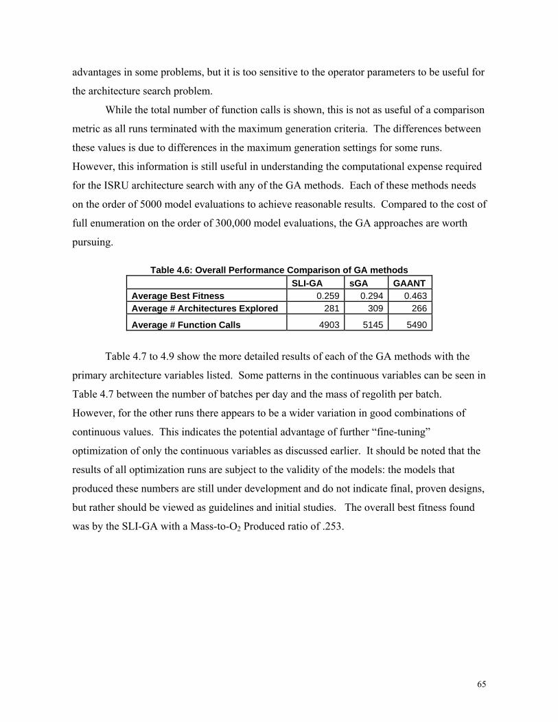
advantages in some problems, but it is too sensitive to the operator parameters to be useful for
the architecture search problem.
While the total number of function calls is shown, this is not as useful of a comp
metric as all runs terminated with the maximum generation criteria. The differences between
these values is due to differences in the maximum generation settings for some runs.
However, this information is still useful in understanding the computational expense required
for the ISRU architecture search with any of the GA methods. Each of these methods needs
on the order of 5000 model evaluations to achieve reasonable results. Compared to the cost of
full enumeration on the order of 300,000 model evaluations, the GA approaches are worth
pursuing.
Table 4.6: Overall Performance Comparison of GA methods SLI-GA sGA GAANT
arison
Average Best Fitness 0.259 0.294 0.463 Average # Architectures Explored 281 309 266
Average # Function Calls 4903 5145 5490
. Some patterns in the continuous variables can be seen in
4.7 between the number of batches per day and the mass of regolith per batch.
However, for the other ru mbinations of
continuous values. This indi tunin
optim onl continuo s as di rlie t the
results of all optimization ru e subject to the validity o odels: th els
produced these numbers are under deve nt and d indicate final, proven designs,
initial studies. The overall best fitness found
253.
Table 4.7 to 4.9 show the more detailed results of each of the GA methods with the
primary architecture variables listed
Table
ns there appears to be a wider variation in good co
cates the potential advantag
y the
e of
scussed ea
furt -her “fine
r. It should be
g”
noted thaization of us variable
ns ar f the m e mod that
still lopme o not
but rather should be viewed as guidelines and
was by the SLI-GA with a Mass-to-O2 Produced ratio of .
65
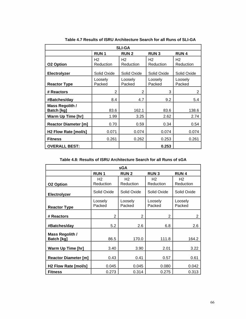
Table 4.7 Results of ISRU Architecture Search for all Runs of SLI-GA
SLI-GA RUN 1 RUN 2 RUN 3 RUN 4
O2 Option H2 Reduction
H2 Reduction
H2 Reduction
H2 Reduction
Electrolyzer Solid Oxide Solid Oxide Solid Oxide Solid Oxide
Reactor Type Loosely Packed
Loosely Packed
Loosely Packed
Loosely Packed
# Reactors 2 2 3 2
#Batches/day 8.4 4.7 9.2 5.4MasBatch [k
s Regolith / g] 83.6 162.1 83.6 138.6
Warm Up 2.74 Time [hr] 1.99 3.25 2.62
Reac meter [m] 0.70 0.54tor Dia 0.59 0.34
H2 Fl 0.071 0.0ow Rate [mol/s] 74 0.074 0.074
Fitne 0.26ss 0.261 2 0.253 0.261
OVERALL BEST: 0.253
Table 4.8: Results of ISRU Architecture Search for all Runs of sGA
sGA RUN 1 RUN 2 RUN 3 RUN 4
O2 Option H2
Reduction H2
Reduction H2
Reduction H2
Reduction
Electrolyzer Solid Oxide Solid Oxide Solid Oxide Solid Oxide
Reactor Type Loosely Packed
Loosely Packed
Loosely Packed
Loosely Packed
# Reactors 2 2 2 2
#Batches/day 5.2 2.6 6.8 2.6
Mass Regolith / Batch [kg] 86.5 170.0 111.8 164.2
Warm Up Time [hr] 3.40 3.90 2.01 3.22
Reactor Diameter [m] 0.43 0.41 0.57 0.61
H2 Flow Rate [mol/s] 0.045 0.045 0.080 0.042Fitness 0.273 0.314 0.275 0.313
66
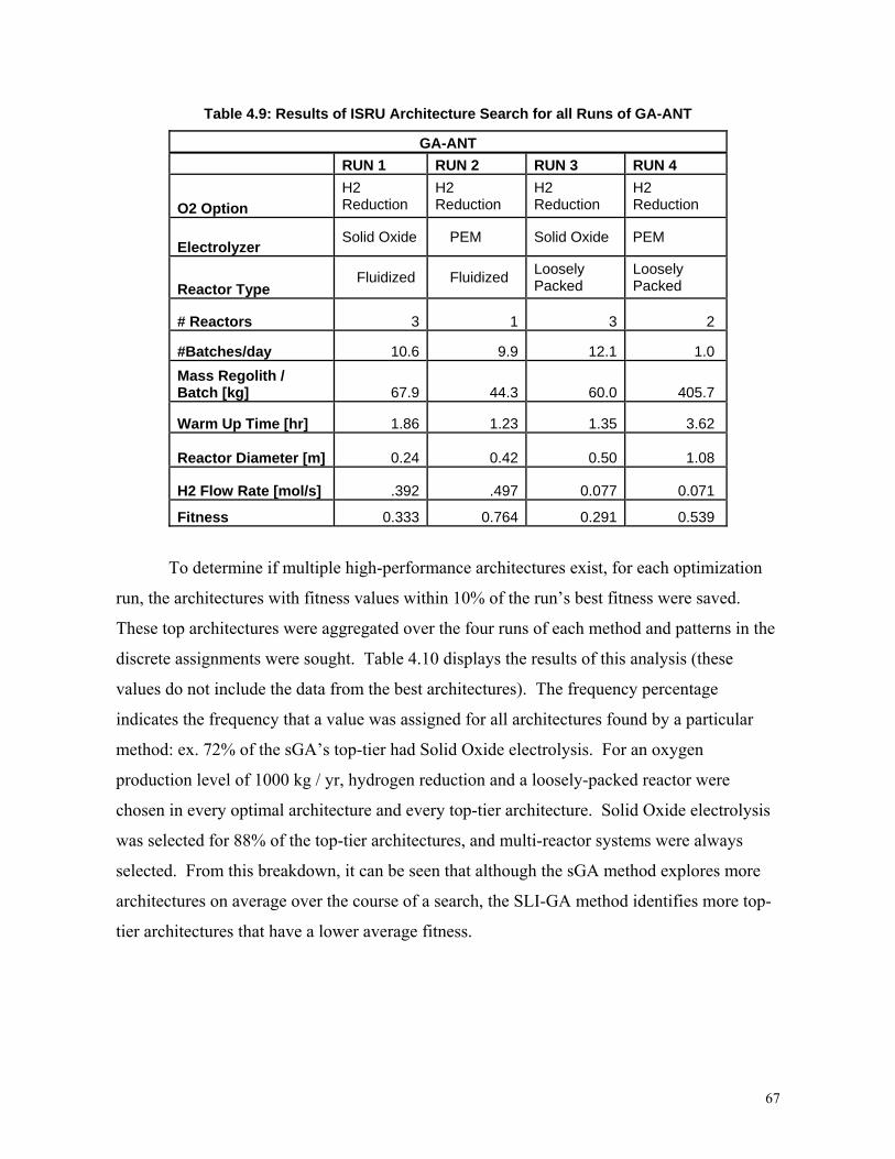
Table 4.9: Results of ISRU Architecture Search for all Runs of GA-ANT
GA-ANT RUN 1 RUN 3 RUN 4 RUN 2
O2 Option n HR n
HR n
HR n
H2 Reductio
2 eductio
2 eductio
2 eductio
Electrolyzer Solid Oxide S PPEM olid Oxide EM
Reactor Type LP
LPFluidized Fluidized oosely
acked oosely acked
# Reactors 3 1 3 2
#Batches/day 10 9 12 1.6 .9 .1 .0 Mass Regolith /
Batch [kg] 6 6 47.9 44.3 0.0 05.7
Warm Up Time [hr] 1 1 1 3.86 .23 .35 .62
Reactor Diameter [m] 0 0 0 1.24 .42 .50 .08
H2 Flow Rate [mol/s] .392 .497 0.077 0.071
Fitness 0.333 0.764 0.291 0.539
To determ timization
run, the architectures with fitness values within
These to architectures were ag d over runs method and patterns in the
discrete assignm ts were soug .10 e r is a ese
values do not include the data f architectures). The frequency percentage
indicates the frequency that a value was assigned for all architectures found by a particular
method: ex. 72% of the sGA’s top-tier had Solid Oxide electrolysis. For an oxygen
production level of 1000 kg / yr, hydrogen reduction and a loosely-packed reactor were
chosen p-tier hitecture. id Oxide e olysis
was selec tier architectures, and multi-reactor systems were always
selected breakdown, it can b n that a h the sG thod explores more
architectures on average over the course of a search, the SLI-GA m identifie re top-
tier arch wer average fitness.
ine if multiple high-performance architectures exist, for each op
10% of the run’s best fitness were saved.
p gregate the four of each
en ht. Table 4 displays th esults of th nalysis (th
rom the best
in every optimal architecture and every to arc Sol lectr
ted for 88% of the top-
. From this e see lthoug A me
ethod s mo
itectures that have a lo
67
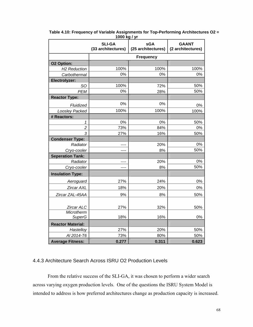
Tab tures O2 = 1000 kg /
A (33 cture
sG archite
GAANT (2 ar res)
le 4.10: Frequency of Variable Assignments for Top-Performing Architecyr
SLI-G archite
s) (25
A ctures) chitectu
Frequency O2 Option:
H2 Reduction 0% 100% 10 100%Carbothermal 0% 0% 0%
Electrolyzer: SO 100% 72% 50%
PEM 0% 28% 50% Reactor Type:
Fluidized 0% 0% 0% Loosley Packed 100% 100% 100%
# Reactors: 1 0% 0% 50% 2 73% 84% 0% 3 27% 16% 50%
Condenser Type: Radiator ---- 20% 0%
Cryo-cooler ---- 8% 50% Seperation Tank:
Radiator ---- 20% 0% Cryo-cooler ---- 8% 50%
Insulation Type:
Aeroguard 27% 24% 0% Zircar AXL 18% 20% 0%
Zircar ZAL-45AA 9% 8% 50%
Zircar ALC 27% 32% 50% Microtherm
SuperG 18% 16% 0%
Reactor Material: Hastelloy 27% 20% 50%
Al 2014-T6 73% 80% 50% Average Fitness: 0.277 0.311 0.623
4.4.3 Architecture Search Across ISRU O2 Production Levels
the relative success of the SLI-GA, it was chosen to perform a wider search
across varying oxygen production levels. One of the questions the ISRU System Model is
intended to address is how preferred architectures change as production capacity is increased.
From
68
Optimiz
The best architectures out of each o run along with the top-tier arch
shown in Figure 4.6 as a production curve. The s d power
factor) is plotted against the actual production rate of each architecture. The best architectures
forming o n as red d ds with a power-law curve fit. Several points
can be taken f : 1. solid oxide trolysis seems o to trade well a
production levels of near 1000 kg/yr; 2. production levels above 2000 kg/yr almo have 3
reactors (first number in the legend labels), ere may be an economy of scale with ISRU
plants.
For p above 5000 2 ction
constraint. The 6000, 7000, and 8000 runs all maxed out around 5 00 kg/yr, with th
exception of the only Carbothermal archite
large jump in system mass. This implies e penalty incu for violation of the O2
constraint is better than the performance of architectures that do satisfy the constraint. The
system may have a phase-shift point above uction levels of 0 kg/yr to a s r slope.
To try to fil on of the curve out more, three ad al runs were p rmed
with the O constraint violation penalty increased. This forced constraint to b
the best results of these runs at O2 = 6500 kg/yr are included on
Because of the ± s on the O2 co int, the actual O els are around 0 kg/yr.
While all th s additional pen were able to m 2 constraint, only one
run resulted in feasible designs: the rest violated one of the time constraints. Curiously, for all
previous runs, higher production levels caused a shift to only use of three reactors, indicating
that more reactors operating in tandem are preferable. However, the best and top-tier
architectures for th al 6500 kg/yr ad a mix of one and two reactors
Further exploration of this region should be performed to ascertain the im of
reactor numbers, with more runs including the larger penalties for violation of the O2
constraint. Further development of the models may also be necessary to better capture the
e search can not only
inform designers on specific ar
ation runs with the SLI-GA were performed for rates from 1000 kg/yr to 8000 kg/yr.
ptimization itectures are
ing the electrical ystem mass (exclu
a Pareto front are sh w iamon
rom this figure elec nly t lower
st all
3. th
roduction levels kg/yr, the GA could not satisfy the O Produ
5 e
cture selected in the 7000 run, which shows the
that th rred
prod 500 teepe
l this regi dition erfo
2 the e met, and
the plot in Figure 4.6.
10% bound nstra 2 lev 680
ree runs with thi alty eet the O
e addition run h .
pacts
multi-reactor system effects. In this way, the preliminary architectur
chitectures to investigate with more detailed design, but can
also be used to guide the system model development and point to interesting areas of the trade
space.
69
From the initial search results, to satisfy the ~1500 kg / yr crew oxygen requirement
for a lunar base, a 1500 kg/yr plant would cost approximately 300 kg of system mass. This
appears very attractive, but does not include the electrical power system or the excavation
rovers needed to deliver regolith to the plant. However, these additions are also components
that may serve dual purposes with other lunar base systems: rovers may be designed to build
up a stockpile of regolith once a week, and spend the rest of their operation time performin
non-ISRU tasks. Similarly, the electrical power system may piggy-back off of the lunar cargo
lander vehicle. Because these higher-level mission architecture options are not yet decided
upon, the
g
multi-use nature of some ISRU components is difficult to assess. These initial
analyse
or capa
)
(4.11)
y of scale, as there is always some fixed-cost of
producing a plant. It is the value of α that is important, as it indicates how the cost-increase
s do indicate that inclusion of ISRU could “pay-off” within less than one year of
operation, provided system reliability is high.
The set of Pareto front designs were fit with a power-law equation to determine if an
economy of scale is present. Economy of scale is a concept generally considered when
planning the rate and quantity of capacity addition to existing systems such as power plants
and chemical production plants. It exists when the per-unit-cost of a plant decreases as output
city increases [Lieberman '87]. A commonly used model to quantify this is shown in
Eqn 4.10, with the empirically fit coefficients from Figure 4.6 shown in Eqn 4.11.
αNkC ∗= (4.10
Where:
C = investment cost
k = scaling constant
N = production quantity per unit time
α = scale coefficient
Pareto front production-cost function: 782.869. NC ∗=
Values of α with 0 ≤ α < 1 exhibit economy of scale. It should be noted that this
model allows investment cost to approach zero as capacity approaches zero. In practice, there
is an operational range for applying econom
70
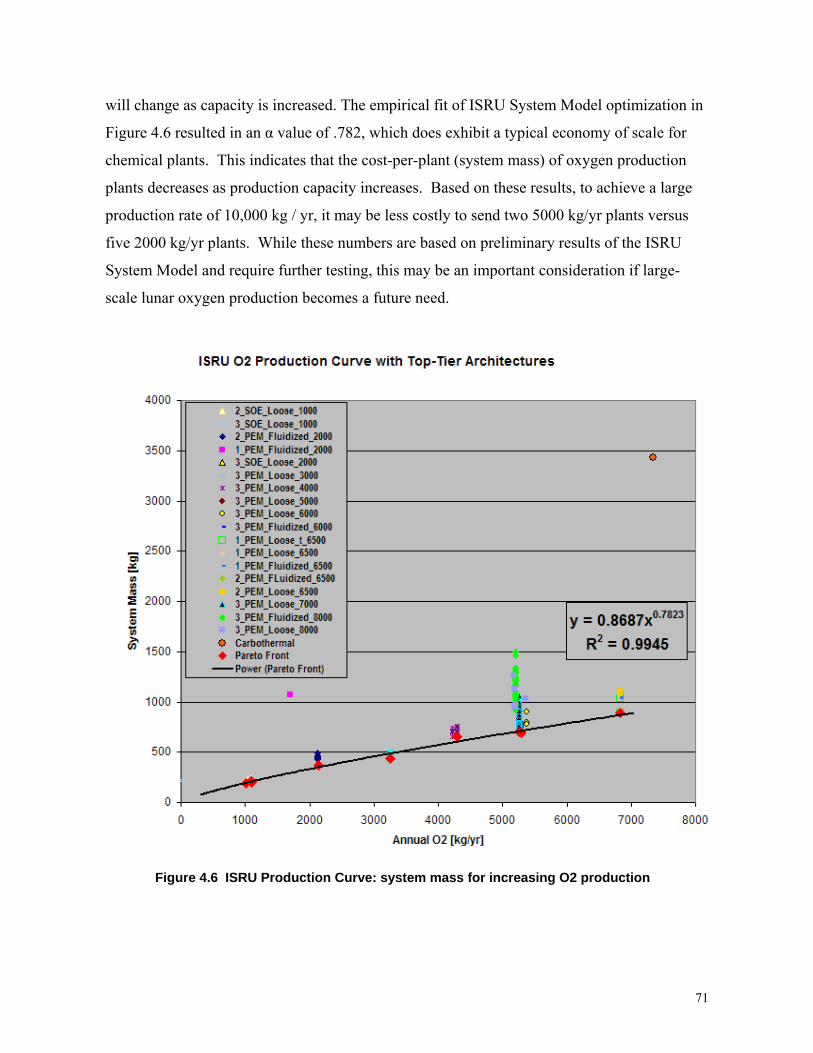
will ch
ange as capacity is increased. The empirical fit of ISRU System Model optimization in
Figure 4.6 resulted in an α value of .782, which does exhibit a typical economy of scale for
chemical plants. This indicates that the cost-per-plant (system mass) of oxygen production
plants decreases as production capacity increases. Based on these results, to achieve a large
production rate of 10,000 kg / yr, it may be less costly to send two 5000 kg/yr plants versus
five 2000 kg/yr plants. While these numbers are based on preliminary results of the ISRU
System Model and require further testing, this may be an important consideration if large-
scale lunar oxygen production becomes a future need.
Figure 4.6 ISRU Production Curve: system mass for increasing O2 production
71
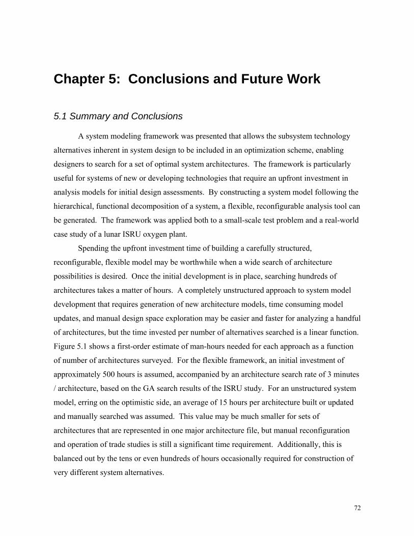
Chapter 5: Conclusions and Future Work
5.1 Summary and Conclusions
A system modeling framework was presented that allows the subsystem technology
alternatives inherent in system design to be included in a
n optimization scheme, enabling
designers to search for a set of optimal system architectures. The framework is particularly
is
balanced out by the tens or even hundreds of hours occasionally required for construction of
very different system alternatives.
useful for systems of new or developing technologies that require an upfront investment in
analysis models for initial design assessments. By constructing a system model following the
hierarchical, functional decomposition of a system, a flexible, reconfigurable analysis tool can
be generated. The framework was applied both to a small-scale test problem and a real-world
case study of a lunar ISRU oxygen plant.
Spending the upfront investment time of building a carefully structured,
reconfigurable, flexible model may be worthwhile when a wide search of architecture
possibilities is desired. Once the initial development is in place, searching hundreds of
architectures takes a matter of hours. A completely unstructured approach to system model
development that requires generation of new architecture models, time consuming model
updates, and manual design space exploration may be easier and faster for analyzing a handful
of architectures, but the time invested per number of alternatives searched is a linear function.
Figure 5.1 shows a first-order estimate of man-hours needed for each approach as a function
of number of architectures surveyed. For the flexible framework, an initial investment of
approximately 500 hours is assumed, accompanied by an architecture search rate of 3 minutes
/ architecture, based on the GA search results of the ISRU study. For an unstructured system
model, erring on the optimistic side, an average of 15 hours per architecture built or updated
and manually searched was assumed. This value may be much smaller for sets of
architectures that are represented in one major architecture file, but manual reconfiguration
and operation of trade studies is still a significant time requirement. Additionally, this
72
Four system architecture optimization methods that addressed both the discrete
architecture design space and the architecture-specific continuous sizing parameters were
tested on the Quadratic Tree test problem and NASA’s ISRU System Model. The
optimization methods each handled compatibility constraints, hierarchical constraints between
technology selections, and subsystem interdependencies. For systems with well-characteri
continuous design spaces and low-complexity architecture hierarchies, the Nested-GA and
full enumeration are feasible and perform with high-confidence in finding a global minimum.
These performed well on the Quadratic Tree test problem. However, on a more complex,
real-world design problem, these two approaches were found to be too computation
expensive to use.
The two single-level GA chromosome representations, sGA and SLI-GA, perform
consistently well on both problems. The sGA performed slightly better on the Quadratic Tree
problem, but the SLI-GA was able to f
zed
ally
ed
ind lower fitness architectures in the ISRU case study.
Figure 5.1: Time investment in architecture search with different modeling approaches.
73
Based on the results of the ISRU architecture search, in terms of performance, the SLI-GA
representation is preferable. The main disadvantage of this method is the custom logic needed
to handle compatibility constraints.
The sGA performs well, but for more complex hierarchies and larger continuous
spaces, the chromosome string becomes exceptionally long, leaving a majority of “junk
DNA”. There is a greater percentage of inactive genes with deeper hierarchies compared to
broader hierarchies. The number of “OR” levels, and choices in each “OR” level dictate the
number of inactive genes. While some authors argue that this better mimics biological
systems, the sGA performance on the ISRU problem indicates that finding good architectures
is more difficult with larger percentages of inactive genes. The sGA can, however, be
flexibly programmed with compatibility constraints, so for changing systems incorporating
many compatibility constraints, the sGA is a preferable method to use.
The dual-agent GA-ANT method performed poorly on both test problems. It was
found that the algorithm’s performance was sensitive to settings of the fitness cut-off values
and mutation rates. More testing may extract better performance from this approach, but
because the other methods already performed well, further work on the GA-ANT method was
limited.
The architecture search of the ISRU System Model yielded a few results of interest,
althoug
sis, while
aint
nalties. This may mean one of a few things: that the bounds on the
model
h all results and values presented in this paper are based only on preliminary
component models and require further validation. It was found that lower production rates
favor architectures with hydrogen reduction, two reactors, and solid oxide electroly
PEM electrolysis was selected more often at production levels over 1000 kg/yr. Multi-reactor
systems tended to be favored at higher production levels, though a few single-reactor systems
traded well at 6500 kg/yr with the reinforced O2 constraint. A power-law fit to the Pareto
front of the architecture production curve indicated that an economy of scale of around .78
may exist for ISRU plants, a level typical of terrestrial chemical plants.
Production rates larger than 5000 kg/yr could not satisfy the O2 production constr
without additional pe
input variables need changing—perhaps allowing a greater number of reactors would
enable more feasible systems; a different approach to handling all continuous constraints may
enforce feasibility better; or that at higher production levels a phase shift in the architecture
74
space may exist. Stronger enforcement of the O2 constraint yielded results that followed the
power-law economy of scale trend of the lower production levels, so there is promise that low
mass-ratio architectures can be found
at higher production rates. Only one architecture to use
the Car at
ugh
un
anging design
environ
e analyzed in greater detail.
this
chromosome formulations. Deeper trees would have a greater proportion of “unused DNA”
bothermal process was selected in any of the final output of the runs, and this was
higher production levels. It was the only architecture to reach feasibility without the
additional O2 constraint. Further testing is needed to determine if Carbothermal trades better
in this region of the production curve.
The ISRU case study demonstrated that a single-level, combinatorial search thro
the architecture and continuous design space is feasible and can provide meaningful results
that designers may otherwise miss when performing trade studies by hand. While the r
times for the GAs take several hours, even with a handful of runs it was shown that
information about the architecture space can be gathered. In a rapidly-ch
ment, there is always a trade-off between time invested in generating analyses and
quality of the results. The GA architecture search methods provide a compromise between
these drivers, assessing over 250 different architectures within the ISRU trade space in one
run. These tools can be used to identify high-performance regions of the design space that
can then b
5.2 Future Work
Future work on the modeling framework and architecture search methods includes
experimenting on test problems with different tree structures. Each of the problems tested in
this paper had only three layers in the hierarchy. This was chosen because for engineering
systems analysis, a hierarchy deeper than three layers does not make much sense for an early-
stage analysis. At deeper layers, smaller-impact variables come under consideration that are
more efficiently explored by first exploring the broader architecture space. From
exploration, a few promising designs can be selected and more detailed analysis and
optimization can focus on the deeper layers.
In terms of hierarchical problem representations in GA’s, however, it would be an
interesting study to determine if the larger segmentation in the chromosome that comes with
more layers of “switch” genes, or hierarchical constraints, would be more difficult for some
75
in each chromosome, potentially making it take longer to converge. Broader trees may have
more difficulty arriving at good continuous variable combinations due to increased subsystem
interaction, but the chromosome representation is more straightforward for the simple GA
operations to have an effect on.
Further testing of the GA-ANT approach should also be performed. Refining
operator parameters may help performance. One issue noted with the GA-ANT convergence
was that with a large number of possible
the
architectures, only one or a limited number of each
architec
er requirements, excavation, crew maintenance and
spare parts mass. Review and verification of the ISRU System Model construction as well as
ates is also necessary for future analysis.
ture species may be present in a population. Enforcing set quantities of species types
to exist in each population may enable a more directed search through continuous space:
without like-species in the population to crossover with, random mutation is the only active
operator.
Future work with the ISRU case study includes a more detailed analysis of the
production curve with more optimization runs at each production level, including the
additional penalty on the O2 constraint to force compliance. Further analysis can be done on
the impacts of ISRU at the mission campaign level by integrating the ISRU architecture
search with SpaceNet for mission-level logistics analysis. This kind of analysis will also
require accounting for ISRU system pow
component model upd
76
References
Armar, N., Siddiqi, A., de Weck, O., Lee, G., Jordan, E., Shishko, R. (2008). “Design of Experiments in Campaign Logistics Analysis”. AIAA Space 2008 Conference & Exposition. San Diego, California, 9-11 Sep. 2008.
Balasubramaniam, R., Hegde, U., Gokoglu, S. (2008). “Carbothermal Processing of Lunar Regolith Using Methane”. Space Technology and Applications International Forum-STAIF 2008, American InstituPhysics.
Belachgar, H., Labib, M., et all (2006). “FERTILE Moon: Feasibility of Extraction of Resources and Toolkit for In-Situ Lunar Exploration”, International Space University, Strasbourg, FR.
Chepko, A., de Weck, O., Linne, D., Santiago-Maldonado, E., Crossley, W. (2008). Architecture Modeling of In-Situ Oxygen Production and its Impacts on Lunar Campaigns.
te of
AIAA Space 2008 Conference & Exposition. San Diego, California, 9-11 Sep. 2008.
Crossley, W. (1995). Using Genetic Algorithms as an Automated Methedology for Conceptual Design of Rotorcraft, Arizona State University. PhD: 31-43.
Dasgupta, D., McGragor, D. (1992). A Structured Genetic Algorithm. R. R. IKBS-2-91, University of Strathc
de Weck O.L., S.-Llyde, UK.
. D., Shishko R., Ahn J., Gralla E., Klabjan D., Mellein J., Shull A., Siddiqi A., Bairstow B,
Eagle En dy: Lee G. (2007). SpaceNet v1.3 User’s Guide, NASA/TP-2007-214725. gineering, I. (1988). Conceptual Design of a Lunar Oxygen Pilot Plant: Lunar Base Systems StuNASA-CR-172082.
Goldberg, D. (1989). Genetic Algorithms in Search Optimization and Machine Learning. Boston, Addison-Wesley Longman.
Graff C., d. W. O. (2006). “A Modular State-Vector Based Modeling Architecture for Diesel Exhaust System Design, Analysis and Optimization”. 11th AIAA/ISSMO Multidisciplinary Analysis and OptimizConference, Portsmouth, Virginia, AIAA-2006-7068.
Hassan, R., Crossley, W. (2003). "“Multi-Objective Optimization of Communication Satellites with Two-BrTournament Genetic Algorithm”."
ation
anch AIAA Journal of Spacecraft and Rockets Vol 40(No 2).
Hegde, U., Balasubramaniam, R., Gokoglu, S. (2008). “Analysis of Thermal and Reaction Times for Hydrogen Reduction of Lunar Regolith”, Space Technology and Applications International Forum-STAIF 2008, American Institute of Physics.
Kirkpatrick, S., C. G. Jr., and M. Vecchi (1983). "Optimization by Simulated Annealing." Science Vol. 220(No
Lieberm , M. (1987). "Market Growth, Economies of Scale, and Plant Size in the Chemical Processing stries." Journal of Industrial Economics
4598): pp. 671-680. anIndu Vol 36(No. 2): pp 175-191.
March, J. 1991). "Exploration and Exploitation in Organizational Learning." Organization Science ( Vol 2(No 1): 1-87.
Mosher, T. (1999). "Conceptual spacecraft design using a genetic algorithm trade selection process." Journal of 7
Aircraft Vol 36(No 1): 200-208. Nadir, W. (2005). Multidisciplinaty Structural Design and Optimization for Performance, Cost, and Flexibility.
eronautics and AstronauticsA . Cambridge, MIT. Masters of Science: 34-37. Papalambros, P., Wilde, D. (2000). Principals of Optimal Design Modeling and Computation. New York,
ambridge University. Parmee, I. C. (1996). The development of a dual-agent strategy for efficient search across whole system
C
engineering design hierarchy. 4th Int. Conf. on Parallel Problem Solving from Nature. Rafiq, M Y. M., J. D., Bullock, G. N. (2003). "Conceptual Building Design-- Evolutionary Approach." Journal .
of Computing in Civil Engineering Vol 17(No 3): 150-158. Sanders, G. (2000). ISRU: An overview of NASA's current development activities and long-term goals. 38th
Aerospace Sciences Meeting & Exhibit, AIAA 2000-1062. Simmon W. (2008). A Framework for Decision Support in Systems Architecting. Aeronautics and s,
Astronautics. Cambridge, MIT. PhD. Steffen, Freeh, J., Linne, D., Faykus, E., Gallo, C., Green, R. (2007). “System Modeling of Lunar Oxygen
roduction: Mass and Power Requirements”. Proceedings of Space Nuclear Conference 2007C., P . Boston,
aper 2049. P
77

Wakayama, S. (2000). “Blended-Wing-Body et-up”. 8th AIAA/USAF/NASA/ISSMO Optimization Problem SSymposium on Multidisciplinary Analysis and Optimization, AIAA-2000-4740.
Watson, ., Hornby, G., Pollack, J. (1998). Modelling Building-Block Interdependency R . Parallel Problem
Solving from Nature- PPSN V, Springer.
Wilcox, K., Wakayama, S. (2003). "Simultaneous Optimization of a Multiple-Aircraft Family." AIAA Journal ofAircraft Vol 40 (No 4).
78
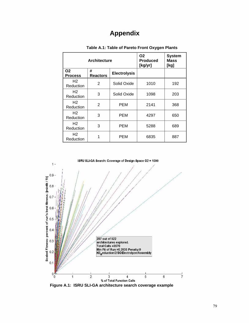
Appendix
Table A.1: Table of Pareto Front Oxygen Plants
Architecture O2 Produced [kg/yr]
System Mass [kg]
O2 Process
# Reactors Electrolysis
H2 Reduction 2 Solid Oxide 1010 192
H2 Reduction 3 Solid Oxide 1098 203
H2 Reduction 2 PEM 2141 368
H2 Reduction 3 PEM 4297 650
H2 Reduction 3 PEM 5288 689
H2 Reduction 1 PEM 6835 887
Figure A.1: ISRU SLI-GA architecture h coverage example searc
79
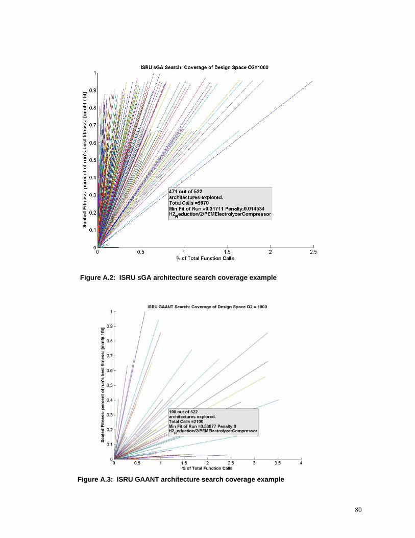
Figure A.2: ISRU sGA architecture search coverage example
Figure A.3: ISRU GAANT architecture search coverage example
80