technology of ehis (stamping) applied to production of ... · technology of ehis (stamping) applied...

Churilova Maria Saint-Petersburg State Polytechnical University

Department of Applied Mathematics

Technology of EHIS (stamping) applied to production of automotive parts

The problem described in this report originated from the joint project of General Motors, USA and the Laboratory of Pulsed Power Energy, and the Laboratory of Applied Mathematics and Mechanics, Saint Petersburg State Polytechnical University, Russia. The project is in progress. Motivation

An application of the discharge in water with the aim of metal forming was firstly described in 40s of the 20th century and then examined experimentally and theoretically since the end of 50s in the Soviet Union and the USA. Since that time this technology has been developed mostly in our country for the purpose to produce small series of items. Nowadays, GM is interested in industrial application of Electro Hydraulic Impulse Stamping (EHIS) to put out small automotive parts.

It is planned to construct a laboratory bench for stamping of small fragments of the automotive parts. An experimental research of the EHIS process is conducted on this bench. A numerical methodology for complex simulation of such process is developed and validated on the basis of experimental data.

The analysis of the previous publications and the available experience give evidence that the electric discharge in water can be effectively used for stamping of the flat-pattern parts. There is a great number of publications with description of the specific technological processes.

An additional investigation is needed including research of the physics of EHIS process, measuring parameters that determine the deformation process (energy, pressure field, material deformation rate, etc.), development of a theoretical model that can interpret the obtained experimental results and relate them to the power supply parameters.

The project is aimed at:

1. Development and validation of numerical methodology, which is capable to simulate the EHIS process. The developed mathematical model of the process should describe the plastic deformation of the plate stock under the action of expanding water. For simulation of the EHIS process it is planned to implement LS-DYNA code.

2. Testing the EHIS process with model hydro-pulse laboratory benches. It is planned to

perform experimental investigations of the process of pressure field forming at the electrical discharge. Moreover, it is necessary to find similarity conditions of EHIS processes for possible scaling of the process.

3. Development of an EHIS technological model for a given object (part). Verification of the

numerical model and similarity conditions at realization of full scale technological process. Description of the technological process

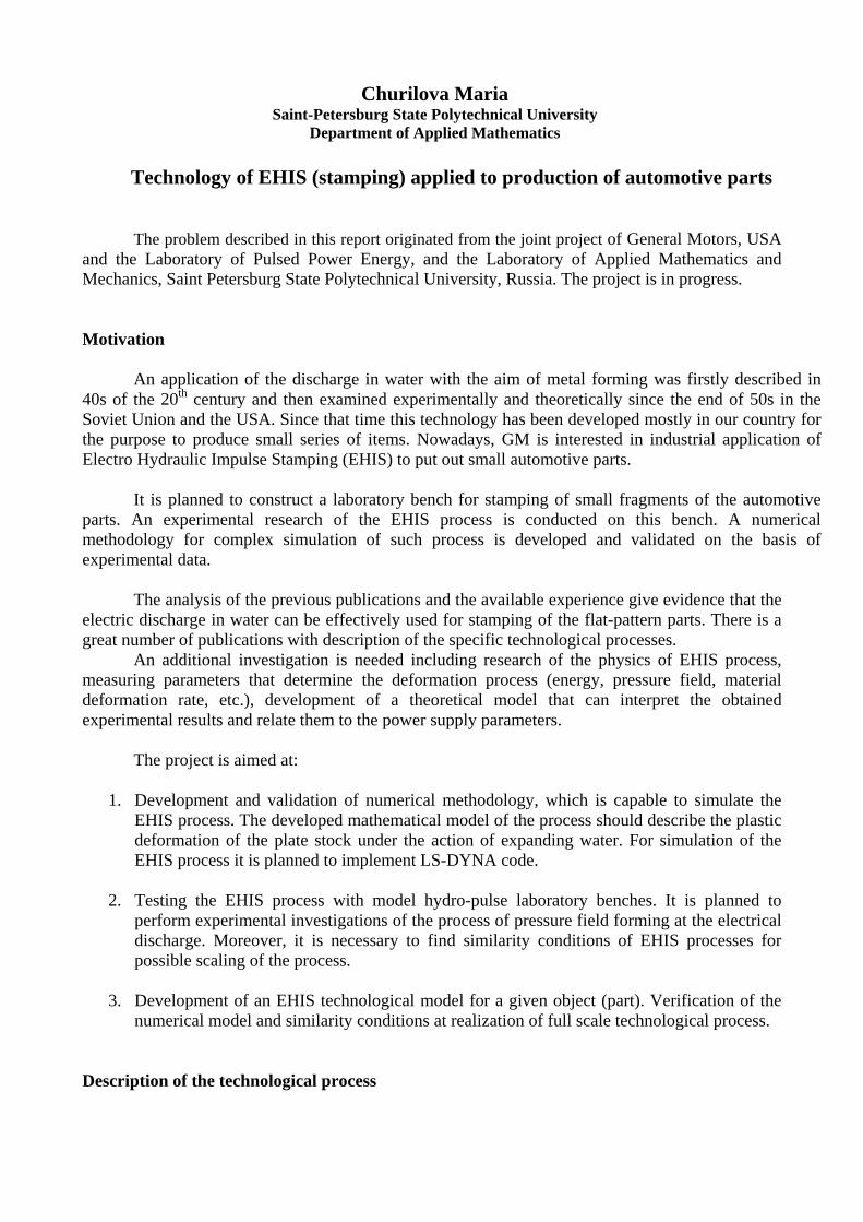
A conventional scheme of the spark discharge experiment in the water is shown in Fig. 1. After closing switch S, the voltage from the charged capacitor C is applied to electrodes 2 located in the discharge chamber 1. The chamber is filled with water. The discharge causes development of a gas bubble and water expansion. The time of discharge development is determined by the characteristics of the discharge gap. Usually, it is from to seconds. 510− 410−

Fig. 1. Experimental plant

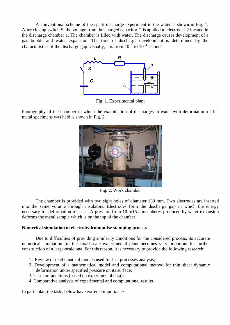
Photography of the chamber in which the examination of discharges in water with deformation of flat metal specimens was held is shown in Fig. 2.

Fig. 2. Work chamber

The chamber is provided with two sight holes of diameter 130 mm. Two electrodes are inserted

into the same volume through insulators. Electrodes form the discharge gap in which the energy necessary for deformation releases. A pressure from 10 to15 atmospheres produced by water expansion deforms the metal sample which is on the top of the chamber. Numerical simulation of electrohydroimpulse stamping process

Due to difficulties of providing similarity conditions for the considered process, its accurate numerical simulation for the small-scale experimental plant becomes very important for further construction of a large-scale one. For this reason, it is necessary to provide the following research:

1. Review of mathematical models used for fast processes analysis; 2. Development of a mathematical model and computational method for thin sheet dynamic

deformation under specified pressure on its surface; 3. Test computations (based on experimental data); 4. Comparative analysis of experimental and computational results.

In particular, the tasks below have extreme importance

1. Determination of constitutive relationships for the materials to be used; 2. Adaptation of a computational model in accordance to the specific material characteristics; 3. Estimation of influence of possible inaccuracy in model parameters on the difference

between computational and experimental results. Research method

The electrohydroimpulse stamping of metals is a complicated process, which is characterized by development of several physical phenomena and their interaction in time. An additional complexity in simulation of such process is related to the fact that the deformation of a blank may lead to significant changes in the model geometry.

Elaboration of any stamping technology requires some estimation for stamping process parameters and development of corresponding mathematical models, which are able to represent real-life physical phenomena adequately.

Capabilities of modern engineering software (ANSYS, LS-DYNA, etc.) for providing accurate and adequate simulations to the process of elastoplastic metal deformation are wide. It is well known, that LS-DYNA is able to provide accurate results for simulation of a fast metal stamping process, but there are only a few articles where such an approach is described in application to electrohydroimpulse forming of metals. In our opinion, usage of LS-DYNA for all stages of simulation (such as selection of a material model, loading, solution, and post processing of the results) based on comparison to experimental data is a right way of constructing methods for mathematical modeling of EHIS. Physical phenomena of metal deformation, which are necessary to take into account For successful stamping, it is necessary to achieve a high level of plastic deformations, therefore a model of plasticity becomes very important. This model should be suitable for simulation of plastic behavior of a metal as well as for simulation of a hardening. Governing system of equations for description of a blank motion is the following:

divu fρ σ ρ= +&& , where u is the displacement vector, ρ is the current density (a function of spatial coordinates only), σ is the Cauchy stress tensor, and is the body force density. For any model, this system should be completed by boundary conditions for tractions and displacements, and by a constitutive relationship of the form

f

( )σ σ ε= , where ε is the total strain tensor, which is the sum of elastic and plastic parts, i.e.

.e pε ε ε= + For example, for a linear elastic material the constitutive relationship has the form

, eDσ ε ε ε= = , where D is the tensor of elastic moduli. Plasticity

A well-known type of tests to analyze the behavior of a material is the tension of a rod (see Fig. 1). The result of such test is represented by plotting the ratio of tensile stress to the initial cross-sectional area, against some measure of the total strain.

If the length of a tensile specimen is increased from to l the amount of deformation is measured as

0l)/ln( 0ll=ε (called logarithmic or natural strain) or as 00 /)( lll −=ε (engineering or

conventional strain); they are approximately identical when the change in length is small, but as the strain increases natural strain becomes progressively less than engineering strain.

Fig. 3. Tension of a rod

Most common engineering materials exhibit a linear stress-strain relationship up to a stress level known as the proportional limit (Point A). Beyond this limit, the material behavior becomes nonlinear, but not necessarily inelastic. Plastic behavior begins when stresses exceed the material's yield point (i.e., the stress level corresponding to Point B).

Fig. 4. Typical stress-strain relationships for metals

(a) – soft metal (copper), (b) – hard metal (steel)

A – proportional limit B – yield point C – point where hardening starts DE – unloading, EF – repeated loading Because there is usually a small difference between the yield point and the proportional limit, it is typically assumed that these two points are coincident in plasticity analyses. From Point B up to Point C the stress remains stable and only deformation increases (see diagram (a)).

For some metals there is no curve interval BC and after Point B the hardening of a material starts immediately (see diagram (b)). It is called “hardening” because after unloading and repeated loading yielding limit increases. Processes of unloading and repeated loading are also shown in both diagrams (curves DE and EF, respectively). For simplified mathematical models of plasticity it is usually assumed that these curves are parallel to the starting linear curve OA. Yield criterion

The yield criterion determines the stress level at which yielding begins. For multi-component stresses, it is represented through the definition of the yield function )(σF of the stress tensor σ .

For many cases, this function is interpreted as a function of the equivalent (von Mises)

stress23

2D

Eσ σ= . Here is the deviator of the tensor D Pσ σ= + Ι σ , where Ι is the identity

tensor, tr3

P σ= − is the pressure and D D D

ij ijσ σ σ= . When the equivalent stress is equal to a

material yield parameter Yσ , the material will develop plastic strains. If Eσ is less than Yσ , the material is elastic, and stresses develop according to the elastic stress-strain relationship.

Fig. 5. Stress-strain relations for the simplest mathematical models of plasticity

Case (a) corresponds to the perfect plasticity (no hardening), and Case (b) represents behavior with linear hardening where there are two linear parts of the stress-strain curve. Yield surface

In case of a complicated stress state for description of a yielding start conditions it is necessary to input yield function . Stress is considered to be acceptable ifF ) ≤(σF 0 . That surfaces, for which 0)( =σF , are called yield surfaces. Any stress state corresponding to the point inside yield surface can be reached purely with elastic deformations. Plastic deformations occur only if

0)( =σF((on the yield surface). In case of a perfect plasticity yield surface remains constant. Area

where 0) <σF is called the elastic area, and area where 0)( =σF is called the plastic one. A material element is said to be in an elastic state if )( 0<σF , and in a plastic state

when 0)( =σF . For plastic yielding, the element needs to be in a plastic state ( ), and to

remain in a plastic state ( ); otherwise the plastic strain rate

0=F

0 p=F& pijp

ijε ε ε& &=&

0pε

vanishes (in common plasticity theory time is not taken into account, but it is used as a parameter which controls the loading process, then dot means the time derivative). Hence =& for or (0<F 0=F and

); otherwise there is a yielding. The first condition corresponds to the case when element is in an elastic state, second – to the case when element passes from a plastic state to an elastic state (unloading). For metal under not very high pressure yield function depend not on stress tensor but on its deviator. In this case, yield surface can be defined with equation (von Mises criterion)

0<F&

221( ) 02 3

D YF σσ σ= − = .

In principal stress space 32 ,1 , yield surface will look like a cylinder with axis 31σ σσ 2σ σσ == which is perpendicular to the deviatoric plane (where tr 0σ = ). In projection on a deviatoric plane, yield surface looks like a circle with center in the origin.

Fig. 6. Yield surface for von Mises criterion

Hardening

For metals under plastic deformations, yield limit increases with deformation growth. It means that the value of the parameter Yσ increases. Metal gains additional elastic properties, and loses ability to deform plastically. This phenomenon is called hardening. The hardening rule describes how the yield surface changes with progressive yielding, so that the conditions (i.e. stress states) for subsequent yielding can be established.

In work hardening, the yield surface remains centered about its initial centerline and expand in size as the plastic strains develop (see Fig. 7 where the projection of the yield surface to the deviatoric plane is shown). This option is preferable for our analysis due to the necessity to include large strains into a model.

Fig. 7. Yield surface expansion in the model with isotropic hardening

ANSYS LS-DYNA plasticity models Bilinear Isotropic Model (BISO)

This classical strain rate independent bilinear isotropic (work) hardening model uses two slopes (elastic and plastic) to represent the stress-strain behavior of a material (see Fig. 5(b)). Stress-strain behavior can be specified at only one temperature (a temperature dependent bilinear isotropic model is also available). Input elastic parameters are elastic modulus E (the tangent slope to the first part of the stress-strain curve in Fig. 5(b)), Poisson’s ratio, and density of a material. The program calculates the bulk modulus using the elastic modulus and Poisson’s ratio values. Input parameters for the simulation of a plastic behavior are the initial yield limit 0Yσ and the tangent slope Etan to the second (plastic) part of the stress-strain curve in Fig. 5(b). A material anisotropy is not supported for this model.

The constitutive relationships for this model are given for rates (or small increments) of displacements, stresses and strains. The von Mises criterion of yielding is used. The system of corresponding relations have the form

( )1 ,2

( ),

,

e p T

p

pD

d d d du du

d D d dFd

ε ε ε

σ ε ε

ε λσ

= + = ∇ +∇

= −∂

=∂

where λ is a plastic multiplier which vanishes for elastic state and unloading. For any iteration of the solution process, using the so-called plastic tangent modulus

tan

tanP

EEEE E

=−

,

ANSYS LS-DYNA calculates the current value of the hardening parameter as 0( )p p

Y eff Y p effEσ ε σ ε= + ,

where 0

tp

eff effd pε ε= ∫ is the current value of the effective plastic strain (which is also called the

equivalent plastic strain), and the effective plastic strain increment is given by the formula 23

p peff ij ijd d pdε ε ε= .

From two formulas above follows, that during the calculation process it is necessary to save into memory the time history only for the effective plastic strain. The value of λ for every small substep of loading comes from the plastic yielding condition

0ij

DYD

ìj Y

F FdF d dσ σσ σ∂ ∂⎛ ⎞= +⎜ ⎟∂ ∂⎝ ⎠

= ,

where

,D pY p eD

F d E d ffσ σ εσ∂

= =∂

.

The last relation is also used for calculation of increment for hardening parameter. Taking into account the above-mentioned explicit form of the function F and the relation

: :D D D D Dij ijd d dσ σ σ σ σ= = σ ,

we arrive at the expression

( )2 2: :3 3

D p D pY p eff Y p effd E d D d d E dσ σ σ ε σ ε ε σ ε− = − − 0p =

or 22 2: :

3 3D D D

Y pDd D Eσ ε λ σ σ σ σ⎛ ⎞

= +⎜ ⎟⎜ ⎟⎝ ⎠

D .

Therefore

2

:2 2:3 3

D

D D DY p

Dd

D E

σ ελσ σ σ σ

=+

.

Johnson-Cook model

This model, also called the viscoplastic model, is a strain-rate and adiabatic (heat conduction is neglected) temperature-dependent plasticity model. This model is suitable for problems where strain rates vary over a large range.

Johnson and Cook express the yielding limit as

( )( )*

0

( ( ) ) 1 ln 1p

meffp ny effA B c T

εσ ε

ε⎛ ⎞

= + + +⎜ ⎟⎜ ⎟⎝ ⎠

&

& , roommelt

room

TTTT

T−−

=* ,

where are material constants, meltTmncBA ,,,,,0

peffεε&

&is the dimensionless plastic strain rate, 0ε& –

the initial strain rate (usually is treated as 1.0 s-1). Input parameters for the simulation are the elastic modulus, Poisson’s ratio, density of a material and all above-mentioned material constants. There is also a part of the model for fracture, but in our case, no fracture was detected. Temperature dependence is neglected due to experimental data that show no heating of a metal after deformation (it is also often neglected because of insufficient experimental material data). Equation of state (EOS)

In the case of the Johnson-Cook model, an equation of state describes relationship between

the pressure P , the specific internal energy E and the relative volume 0V ρρ

= , where 0ρ is the initial

density. If V and E are independent thermodynamic functions it is sufficient to write this equation of state using only one function

),( EVPP = .

There are two suitable types of equations in ANSYS LS-DYNA. They are called “linear polynomial” and “Gruneisen”.

The linear polynomial equation of state has the form ECCCCP )( 4321 μμμ +++= ,

where 10

−=ρρμ is a dimensionless parameter. For expansion process ( 0<μ ), term is set to

zero and equation transforms into

22μC

ECCCP )( 431 μμ ++= . Gruneisen equation of state is used for high pressures. For compressed materials it has the following form:

2 200

022 3

1 2 3 2

1 (1 )2 2 ( )

1 ( 1)1 ( 1)

acP a

S S S

γρ μ μ μEγ μ

μ μμμ μ

⎡ ⎤+ − −⎢ ⎥⎣ ⎦= +⎡ ⎤− − − −⎢ ⎥+ +⎣ ⎦

+ ,

where 0γ is the Gruneisen gamma, and – material constants. For expanded materials the equation becomes

acSSS ,,,, 321

EaCP )( 02

0 μγμρ ++= . If the parameter μ is small, linear polynomial and Gruneisen equations of state are almost identical to each other. It is known from the literature that to achieve the value of μ = 0.2 it is necessary to provide a pressure about 30 GPa, which is much higher than the range of pressures in our experiments. Therefore, the difference between these two models is insignificant (that is approved by computations).

Below we present some results of numerical simulation for copper stamping at three regimes of pressure distributions in time. We also compare numerical results with experimental results obtained on the small-scale plant. Required data for simulation 1. Geometrical model; 2. Material model; 3. Material properties for a selected material model (density, Poisson’s ratio, elastic modulus, plastic properties and other material constants); 4. Finite Element model based on a selected type of element; 5. Boundary conditions; 6. Loading as a function of time and spatial coordinates; 7. The termination time for simulation; Geometrical and finite element model The model consists of tree parts: the deformable metal blank (cyan), rigid holder (blue) and rigid die (red), 1/4th symmetry was used to reduce the amount of calculations. Blank size: thickness 0.5 mm radius 20 mm The SOLID164 element is used

ANSYS 11.0 APR 8 200915:48:57

1

COMPONENTSSet 1 of 1 _PART1 (Elems)_PART2 (Elems)_PART3 (Elems)

XY

Z

Mesh Near the die edge mesh was refined for accurate computations in area where plastic deformations mostly occur Mesh: 59 349 nodes 50 528 elements

ANSYS 11.0 APR 8 200915:49:59

1

COMPONENTSSet 1 of 1 _PART1 (Elems)_PART2 (Elems)_PART3 (Elems)

Mesh refinement Pressure on the deformable metal blank was measured experimentally and then approximated via sharp or smooth curves. Results of such an approximation are depicted below. Loading (1) Maximum pressure: 1.4 MPa

ANSYS 11.0 APR 8 200915:51:14 mics

1

0

200

400

600

800

1000

1200

1400

1600

1800

2000

(x10**3)

PAR2

0.8

1.62.4

3.24

4.85.6

6.47.2

8

PAR1

(x10**-3)

Plot Explicit Dynamics Curve 4

PAR2

ZV =1 *DIST=.75 *XF =.5 *YF =.5 *ZF =.5 Z-BUFFER

loading curve

Fig. 8. Experimental pressure curve (left), ANSYS LS-DYNA pressure curve (right) The pressure via time curve has tooth-saw peeks. Loading begins not from the zero time but from time about 1.7 milliseconds, but we begin loading from zero. Loading (2) Maximum pressure: 2.5 MPa

ANSYS 11.0 APR 8 200915:52:00 mics

1

0

250

500

750

1000

1250

1500

1750

2000

2250

2500

(x10**3)

PAR2

0.4

.81.2

1.62

2.42.8

3.23.6

4

PAR1

(x10**-3)


PAR2

ZV =1 DIST=.75 XF =.5 YF =.5 ZF =.5 Z-BUFFER

loading curve

Fig. 9. Experimental pressure curve (left), ANSYS LS-DYNA pressure curve (right) Curve was approximated smoothly because of its complex structure. Loading (3) Maximum pressure: 3.3 MPa

ANSYS 11.0 APR 8 200915:52:34 mics

1

0

400

800

1200

1600

2000

2400

2800

3200

3600

4000

(x10**3)

PAR2

0.4

.81.2

1.62

2.42.8

3.23.6

4

PAR1

(x10**-3)


PAR2

ZV =1 DIST=.75 XF =.5 YF =.5 ZF =.5 Z-BUFFER

loading curve

Fig. 10. Experimental pressure curve (left), ANSYS LS-DYNA pressure curve (right)

Material constants for copper Elastic modulus 120.0e9 N/m2

Poisson’s ratio 0.343 Density 8930 kg/m3

Constants for BISO model Yielding limit 70.0e6 N/m2 Tangent slope 2.0e9 N/m2 Constants for Johnson-Cook model Room temperature 27 °C Melt temperature 1083 °C Initial strain rate 1.0 Specific heat 385 Joule / kg °C A 89.63e6 N/m2 B 291.64e6 N/m2 n 0.31 c 0.025 Constants for EOS C1 140e9 N/m2 C2 2.8e9 N/m2 C3 1.96 C4 0.47 Results Maximum deflection for copper blank: max pressure, MPa Experiment, mm BISO, mm Accuracy, % Johnson-Cook, mm 1.4 1.60 1.48 7.5 0.78 2.5 3.00 2.85 5.0 3.3 3.50 3.40 2.9 Time of a typical computation – about 15 hours (AMD Athlon(tm) 64x2 Dual Core Processor 6000+ 3.00 GHz, 3 Gb RAM) Average accuracy for BISO model – 5.1% Johnson-Cook model provides unsatisfactory results. Let consider the last examples in more details.

ANSYS 11.0 APR 9 200912:10:20 NODAL SOLUTIONSTEP=1 SUB =5 TIME=.660E-04 USUM (AVG) RSYS=0PowerGraphicsEFACET=1AVRES=MatDMX =.132E-03 SMX =.132E-03

1

MN

MXXY

Z

0 .147E-04 .293E-04 .440E-04 .586E-04 .733E-04 .879E-04 .103E-03 .117E-03 .132E-03

USUM for the material and set specified

ANSYS 11.0 APR 9 200912:10:39 NODAL SOLUTIONSTEP=1 SUB =10 TIME=.148E-03 USUM (AVG) RSYS=0PowerGraphicsEFACET=1AVRES=MatDMX =.001688 SMX =.001688

1

MN

MX

XY

Z

0 .188E-03 .375E-03 .563E-03 .750E-03 .938E-03 .001125 .001313 .001501 .001688

USUM for the material and set specified Step 5 Time 0.660e-4 sec Step 10 Time 0.148e-3 sec


1

MN

MX

XY

Z

0 .333E-03 .666E-03 .999E-03 .001332 .001665 .001998 .002331 .002664 .002997



1

MN

MX

XY

Z

0 .386E-03 .772E-03 .001159 .001545 .001931 .002317 .002703 .00309 .003476



1

MN

MX

XY

Z

0 .381E-03 .762E-03 .001144 .001525 .001906 .002287 .002669 .00305 .003431



1

MN

MX

XY

Z

0 .382E-03 .765E-03 .001147 .001529 .001911 .002294 .002676 .003058 .003441


Fig. 11. Total displacement via time

On the Fig. 11 we can see how the total displacement changes in time. From these pictures, it follows that the deformation mostly grows up in the period of 1—16 time steps, but the termination time for calculations corresponds to the set number 200. Analyzing the results, we conclude, that from the time step 20 (0.313e-3 sec) only elastic damped oscillations are present. But the amplitude of such oscillations is small enough and we leave them out of account. The accuracy of calculation of the final total displacement is about 3% that is good for engineering purposes.

ANSYS 11.0 APR 9 200912:18:20 NODAL SOLUTIONSTEP=1 SUB =5 TIME=.660E-04 EPPLEQV (AVG) PowerGraphicsEFACET=1AVRES=MatDMX =.132E-03 SMN =.161E-04 SMX =.003247

1

MN

MXXY

Z

.161E-04

.375E-03

.734E-03

.001093

.001452

.001811

.00217

.002529

.002888

.003247

Von Mises plastic strain

ANSYS 11.0 APR 9 200912:18:37 NODAL SOLUTIONSTEP=1 SUB =10 TIME=.148E-03 EPPLEQV (AVG) PowerGraphicsEFACET=1AVRES=MatDMX =.001688 SMN =.563E-03 SMX =.091645

1

MN

MX

XY

Z

.563E-03

.010683

.020803

.030923

.041044

.051164

.061284

.071404

.081524

.091645

Von Mises plastic strain Step 5 Time 0.660e-4 sec Step 10 Time 0.148e-3 sec

ANSYS 11.0 APR 9 200912:19:02 NODAL SOLUTIONSTEP=1 SUB =13 TIME=.198E-03 EPPLEQV (AVG) PowerGraphicsEFACET=1AVRES=MatDMX =.002997 SMN =.001609 SMX =.179163

1

MN

MXXY

Z

.001609

.021337

.041066

.060794

.080522

.10025

.119979

.139707

.159435

.179163



1

MN

MXXY

Z

.003887

.026804

.049721

.072638

.095555

.118473

.14139

.164307

.187224

.210141



1

MN

MXXY

Z

.003141

.026067

.048992

.071918

.094844

.117769

.140695

.163621

.186547

.209472



1

MN

MXXY

Z

.003411

.026291

.049172

.072052

.094932

.117813

.140693

.163574

.186454

.209334


Fig. 12. Von Mises plastic strain via time

The same situation occurs for plastic deformations. They are stable beginning from the time step 20 (0.313e-3 sec). Up to this moment, the total level of plastic deformations is achieved. Conclusions 1. BISO model is more adequate for description of “slow” processes with a moderate pressure. 2. Mean error of the computations with BISO model is about 5%. Plastic deformations occur

where they were expected theoretically. 3. Deformation of a blank in small-scale experimental plant is well simulated by BISO model. 4. Johnson-Cook model is a more complicated and, in our case, it provides worse correlation

with experimental results. Acknowledgments Finally, I wish to thank the head of the Laboratory of Pulsed Power Energy Prof. German Shneerson and his colleagues, and also Assoc. Prof. Sergey Lupuleac and Assoc. Prof. Maxim Frolov, who provided continuous guidance of the present research work.

technology of ehis (stamping) applied to production of ... · technology of ehis (stamping) applied...

Documents