technology learning curve (foak k to o noak) ) library/research/energy analysis... · an aggregate...

August 2013

QQUUAALLIITTYY GGUUIIDDEELLIINNEESS FFOORR EENNEERRGGYY SSYYSSTTEEMM SSTTUUDDIIEESS

TTeecchhnnoollooggyy LLeeaarrnniinngg CCuurrvvee ((FFOOAAKK ttoo NNOOAAKK))

DOE/NETL‐2010/????DOE/NETL‐341/081213

National Energy Technology Laboratory Office of Program Planning and Analysis

1

Technology Learning Curve (FOAK to NOAK) Quality Guidelines for Energy System Studies

August 2013

Disclaimer

This report was prepared as an account of work sponsored by an agency of the United States Government. Neither the United States Government nor any agency thereof, nor any of their employees, makes any warranty, express or implied, or assumes any legal liability or responsibility for the accuracy, completeness, or usefulness of any information, apparatus, product, or process disclosed, or represents that its use would not infringe privately owned rights. Reference therein to any specific commercial product, process, or service by trade name, trademark, manufacturer, or otherwise does not necessarily constitute or imply its endorsement, recommendation, or favoring by the United States Government or any agency thereof. The views and opinions of authors expressed therein do not necessarily state or reflect those of the United States Government or any agency thereof.


2


August 2013

1 Introduction This paper summarizes costing methodologies employed by the National Energy Technology Laboratory (NETL) for estimating future costs of mature commercial Nth-of-a-kind (NOAK) power plants from initial first-of-a-kind (FOAK) estimates for use in costing models and reports. Further, it defines the specific steps and factors that can be used in such estimations. This methodology is based on treating major plant components for various subsystems and obtaining an aggregate learning curve unique to the plant type assessed. Though these guidelines are tailored for power-producing plants, they can also be applied to a variety of different revenue-generating plants (e.g., coal-to-liquids, syngas generation, or hydrogen).

As new technologies are developed and deployed, it is important that decision-makers have a reliable, or at the very least consistent, method of projecting future costs. History shows that subsequent installations will normally cost less than the first plant. Along with lower capital costs, efficiency and reliability will also tend to improve; the latter two elements are not addressed here. However, to some level, when costs, efficiency, and reliability show little or no improvement from one plant to the next, the technology is considered to be mature.

1.1 Definition of Terms

Care is needed in defining FOAK and NOAK. For major new facilities, the number of installations is largely applicable to a specific supplier’s technology. For example, although the gasification technologies are similar, it is unlikely that one vendor will share sufficient experience to benefit rivals such that learning will occur. For example, the ConocoPhillips E-Gas integrated gasification combined cycle (IGCC) system to be installed as part of the Excelsior project is a second-of-a-kind IGCC based on the Wabash project experience, since little or no benefit from other existing plants, such as the Pinon Pine (Kellogg-Rust Westinghouse [KRW]) project, Polk (General Electric Energy [GEE]) project, Buggenum and Puertollano (Shell gas [Shell]) projects, is available to ConocoPhillips in sufficient detail.

Some projects are clearly FOAK based on a new technology. The transport gasifier to be demonstrated in Southern Company’s Clean Coal Power Initiative (CCPI) project falls into this category. Projects that use Nth plant technology in some of the plant, but use large, new, critical subsystems elsewhere should also be considered FOAK. An example of this would be if a gasification technology vendor achieves Nth plant status for IGCC systems and decides to use membrane technology for the air separation unit (ASU) or a solids feed pump for coal delivery in the Nth plus one plant. Not only would these technologies be new, but integration issues may occur and, as such, NOAK may not apply.

An additional issue to consider is that cost reductions do not always begin with the second plant. Here the methods to estimate Nth plant costs (discussed below) tacitly assume that the first plant operates reasonably well and that the main reason for higher FOAK plant costs is a conservative design, fundamentally different from the next installation. In some cases the FOAK plant experience also leads to unpredictable problems and the realization that more components or more expensive components are needed, resulting in the next installation again being fundamentally different. In these cases, the costs may actually increase for the first few installations; here we define the learning responsible for increasing the installation costs as


3


August 2013

mentioned to be due to developmental requirements, as opposed to “learning by doing” which is specifically what this document addresses. This developmental learning is demonstrated by the data presented for selective catalytic reduction (SCR) and flue gas desulfurization (FGD) in Reference 1. When this situation occurs, the FOAK plant may need to be considered as the one where costs reach a maximum. Since these problems are unforeseen, it is impossible to know beforehand when costs will escalate in this manner and so is difficult to treat systematically unless the most expensive installation is considered FOAK.

The definition of the NOAK plant is somewhat arbitrary as well, although it is often taken as the fifth or higher plant. When experience has only a minor effect on further reducing costs, that plant is considered an NOAK plant, where the term “minor” may be specific to the type of installation and relevant market being assessed. Furthermore, there is a point at which minimum plant cost is reached based on the costs of raw materials and components. It should be pointed out that even FOAK plants use mostly NOAK components (e.g., cryogenic ASUs in IGCC).

The impact of time and experience on capital costs is illustrated in Exhibit 1-1. The curves were generated by combining the two methodologies discussed below. The initial upward curve reflects the Engineering-Economic Design Method discussed in Section 2 including contingencies recommended by the Association for the Advancement of Cost Engineering (AACE) International guidelines. [2, 3] The decreasing curve after commercialization reflects the Learning Curve Method described in Section 3. The shaded area surrounding the curve qualitatively reflects the typical level of accuracy associated with design estimates based on the AACE guidelines. [4, 3]

Exhibit 1-1 Typical Impact of Experience on Power Plant Costs

Source: NETL


4


August 2013

1.2 Methodologies

Essentially, there are two approaches to estimating future costs. The first is a traditional engineering-economic design approach based on engineering process models, databases containing previous and current vendor data, standardized factors and indices, and projections by experts in various fields regarding potential improvements in key process and economic parameters. The second is an equation-based approach using mathematical learning or experience curves developed from historical data for similar technologies in similar systems. Both methodologies are described in the following sections.


5


August 2013

2 Engineering-Economic Design Method Costs often decline after a new technology is commercialized as improved versions are built. When the technology is well established and being produced by many vendors in competition with each other, the technology is referred to as “mature.”

Actual capital and operating and maintenance (O&M) cost estimates for specific power generation process equipment and technologies are generated based on detailed design parameters, engineering process models, databases containing previous and current vendor data, standardized factors and indices, and projections by experts in various fields regarding potential improvements in key process and economic parameters. Conceptual cost estimates used in techno-economic studies are typically factored from previous estimation data and are not as accurate as actual detailed estimates. Databases, indices, and conceptual estimating models are maintained as part of plant design bases of experience for similar equipment in power and process projects. The initial values are scaled and modified based on capacity, operating conditions, and application to generate final capital cost estimates for specific installations. Adjustment of costs for capacity and design conditions is a well-established technique and is highly accurate when properly done. [5] NOAK plant costs can be estimated from FOAK costs by applying the expected NOAK design parameter factors and indices along with sound engineering and estimating judgment.

Most techno-economic studies completed by NETL feature cost estimates carrying an accuracy of -15 percent/+30 percent, consistent with a “feasibility study” (AACE Class 4) level of design engineering applied to the various cases. [3, 6, 4] The reader is cautioned that the values generated for many techno-economic studies have been developed for the specific purpose of comparing the relative cost of differing technologies. They are not intended to represent a definitive point cost nor are they generally FOAK values.

Process contingencies are included in estimates to account for “expected but undefined costs” as well as project contingencies which represent costs that are unforeseen due to a lack of complete project definition and engineering. Contingencies are added because experience has shown that such costs are likely, and expected, to be incurred even though they cannot be explicitly determined at the time the estimate is prepared. As technologies mature and estimates progress to more complete design levels, the contingencies are reduced in favor of more defined cost breakdowns. [4]

Many factors can impact the cost of future technology installations even after the technology is commercially mature [7] and this approach takes them into account. Some of the factors are as follows:

Market factors: If demand for a specific technology is high or there is a shortage of materials or manufacturing capacity, costs tend to increase for that technology or its components. If the demand is weak or supply is abundant, costs tend to fall. An “equilibrium” market condition exists in between these two extremes where small changes in demand do not impact costs significantly. [7] Competition, both foreign and domestic, also impacts costs.

Manufacturing factors: Costs for technology components manufactured in large facilities or at large production rates are usually lower than those for limited production versions. Modular


6


August 2013

components such as fuel cells, combustion turbines, and batteries can be expected to be mass-produced. [7]

Scale factors (Typically referred to as economy of scale): Larger equipment tends to cost less per unit of capacity when compared to smaller units. As technologies mature and installed capacity increases, the individual units tend to be larger. [7]

Material price factors: Increases and decreases in costs and availability of raw materials and feedstocks used to manufacture equipment as well as operation and maintenance costs impact the overall costs for a technology or plant. [7]

Inflation factors: Previous cost estimates can be updated to today’s dollars by using cost indices such as Gross Domestic Product (GDP) [8] and Chemical Engineering Plant Cost Index (CEPCI) [9] or other similar factors.

Location factors: Costs for land, labor, transportation, equipment installation, design, and construction (including contractor fees) vary significantly between locations. [7] Installation/construction costs are included in capital estimates and influenced by seismic zone, accessibility, excessive rock, piles, laydown space, etc. Design variations due to elevation, water availability, weather, seismic conditions, etc. also impact estimated cost projections. [6]

Regulatory factors: Taxes, permitting requirements, licensing fees, and government incentives can impact capital cost estimates as well as operating and maintenance estimates. Current and potential future regulation of air, water, and solid waste discharges also impact equipment selection and availability and, therefore, impact demand and final cost values. [7]

Capital costs are dependent on the accuracy and completeness of designs. The most definitive of the estimate techniques are detailed, unit-cost, or activity-based cost estimates that use information down to the lowest level of detail available. [10] Conceptual/factored estimates are dependent on the accuracy of the original estimates. Many of these external factors change from plant to plant, regardless of the maturity level of the technologies. Care should be taken to insure the accuracy of any FOAK estimates and to include all applicable influences when projecting the values to NOAK installation cost values.


7


August 2013

3 Learning-Curve Method The equation approach is based on using mathematical learning or experience curves developed from historical data for similar technologies in similar systems. Learning curves or experience curves are used to predict costs of manufactured products after some experience is gained in their production. They are also applicable to estimating plant costs for subsequent plants using the same technology. These curves are the standard methodology for projecting production costs or constant dollar capital costs based on the first unit or plant costs and are therefore the focus of this paper. While several attempts have been made to develop multi-factored curves, the most commonly used type of curve is based on the premise that some reduction in costs will take place each time the cumulative production is doubled. [11, 12, 13, 14]

This concept is represented mathematically by:

Y=AX-b (1)

Where Y = time or cost to produce Xth unit

A = time or cost to produce the first-of-a-kind unit

X = cumulative number of units, capacity, or ratio of capacities

b = learning rate exponent

The learning rate equation is defined as:

R = (1 – 2-b) (2)

Where R is the learning rate and 2-b is defined as the progress ratio

Solving the learning rate equation for the learning rate exponent results in:

b = - log(1-R) / log(2) (3)

Note - learning rates and progress ratios are reported in literature (as fractions or percentages) or can be derived from historical data. [14, 15]

Exhibit 3-1 graphically demonstrates the rate at which the benefits of experience decline for a number of different learning rates.

The value of R varies from industry to industry, company to company, and can vary from plant to plant within a company. Likewise this value will vary from technology to technology. Thus the learning rate for IGCC will differ from that of fuel cells and the learning rate for E-Gas will possibly differ from that of the GEE gasifier, although one would expect learning rates to be closer for similar technologies. The value assigned for R to a given technology can be based on the experience of estimators within the energy industry.

Complex systems such as power generation facilities consist of many technologies. Each of the technologies can be at a different maturity level. The results of a literature search conducted on power generation process technology cost estimation data yielded two lists of learning rate recommendations shown in Exhibit 3-2 and Exhibit 3-3. [14, 15]


8


August 2013

Exhibit 3-1 Learning Curves for Various Learning Rates

Source: NETL

Exhibit 3-2 Typical R-values Versus Maturity Level

Level of Maturity R - Value

Experimental (FOAK) 0.06

Promising, 2nd 0.05

Growing, 3rd & 4th 0.04

Proven, 5th to 8th 0.03

Successful, 9th to 16th 0.02

Mature, 17th & more 0.01

‐

200

400

600

800

1,000

1,200

‐ 5 10 15 20 25 30 35 40 45 50

Cost of Unit

Units of Installation

R=0.01

R=0.02

R=0.04

R=0.06

R=0.08

R=0.10

R=0.12


9


August 2013

Exhibit 3-3 Recommended R-values for Various Technologies

Cost Category/Technology Type R Value Cost Category/Technology Type R Value

Category 1 Category 5 (cont’d)

Coal Delivery and Handling 0.01 CO2 Capture, Recovery, & Compression 0.03

Category 2 CO2 Transport & Sequestration 0.05

Coal Prep and Feed 0.01 - 0.04* Fuel Cells 0.02 - 0.06**

Category 3 H2 Production 0.02

Feed Water/Misc. BOP 0.01 – 0.05* Direct Liquefaction Process 0.06**

Category 4 0.01 – 0.04 CH4 From Hydrates 0.06**

Boiler Equipment & Aux. 0.01 Category 6 0.01 – 0.05

Gasifier Systems 0.04 - 0.06* Advanced Comb. Turbines 0.04

Syngas Cooling 0.04 Syngas Comb. Turbines 0.05

Air Separation Units 0.03 Hydrogen Comb. Turbines 0.05

O2 Membrane -- N. G. Combustion Turbines 0.01

Category 5 0.02 – 0.05 Category 7

Syngas Cleanup Heat Recovery Systems 0.01

Acid Gas Removal 0.03 Category 8 0.01 - 0.04

Particulate Removal 0.03 Steam Turbines 0.01

Mercury Removal 0.03 Advanced Steam Turbines 0.04

HAPs Removal -- Category 9

Warm Gas Cleanup 0.03 – 0.04* Cooling Towers/Systems 0.01

Sulfur Recovery 0.03 Category 10

Flue Gas Cleanup 0.02 – 0.03 Ash/Slag/Spent Sorbent Handling 0.02

SO2 Removal 0.02 Category 11

NOx Removal 0.02 Power Distribution System 0.01

Particulate Removal 0.02 Category 12

Mercury Removal 0.03 Instruments & Controls 0.01

Haps Removal -- Category 13

Syngas Conversion 0.03 – 0.05 Site Preparation 0.01

Fischer Tropsch Synthesis 0.05 Category 14

Methanol & Ethanol Production 0.03 Buildings & Structures 0.01

Methanation/SNG Production --


10


August 2013

Estimating the Nth plant cost can be done by either applying the learning curve to major components or a plant-wide basis. [14] If it is done on a plant-wide basis, the value selected for R should reflect the mix of mature and immature technologies and the anticipated learning rate for those immature technologies. Thus, a plant consisting largely of immature technologies would normally have a higher value for R than a plant with only a small portion of immature technologies. The difficulty in weighting the various R values for different components can be overcome by estimating each major subsection separately to arrive at a total cost for the Nth plant. The historical data that were analyzed represent past experience and provide some guidance in selecting R value ranges in the final methodology. For the technologies that are represented in typical power plants, the bulk of the learning rates are for technologies that are now NOAK.

This learning-curve methodology is used extensively for applying currently available information to long-term projections based on national and global generation capacities such as those made to study global energy costs for policy-making decisions. [16, 17, 18]


11


August 2013

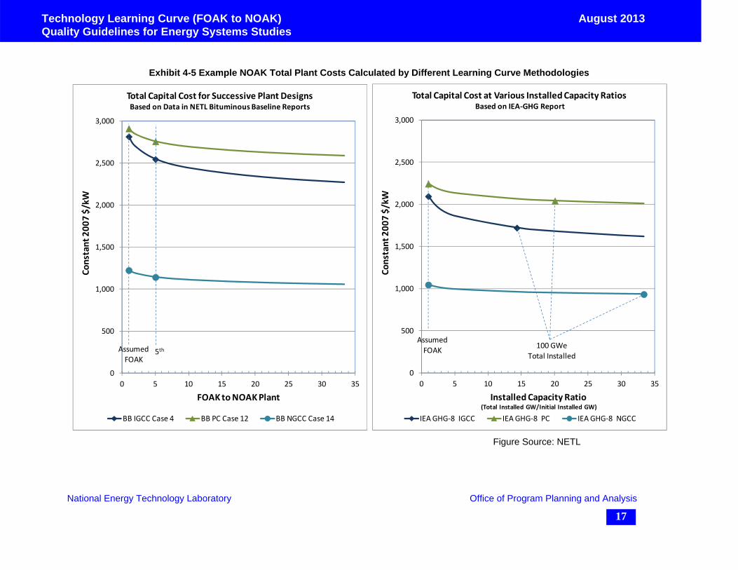
4 Learning Curve Example Calculations The results of three example calculations using the learning curve method are presented in Exhibit 4-1, Exhibit 4-2, and Exhibit 4-3 for IGCC, super-critical pulverized coal (PC), and natural gas combined cycle (NGCC) plants with CO2 capture. The base values were obtained from the Department of Energy (DOE)/NETL Bituminous Baseline Report [6] and assumed as the FOAK plant values for each account. The values for each plant type were estimated (using Equation 1) for the 5th plant, which is typically considered to be the NOAK plant. In reality, each cost account may contain multiple technologies with varying numbers of commercial installations; however this approach assumes that the number of installations represents a weighted average of the technologies in the account. The calculation approach assumes that knowledge is shared with each successive plant installation resulting in improved designs and lowered costs. The overall total plant cost (TPC) for each plant was estimated as the sum of the values for each account.

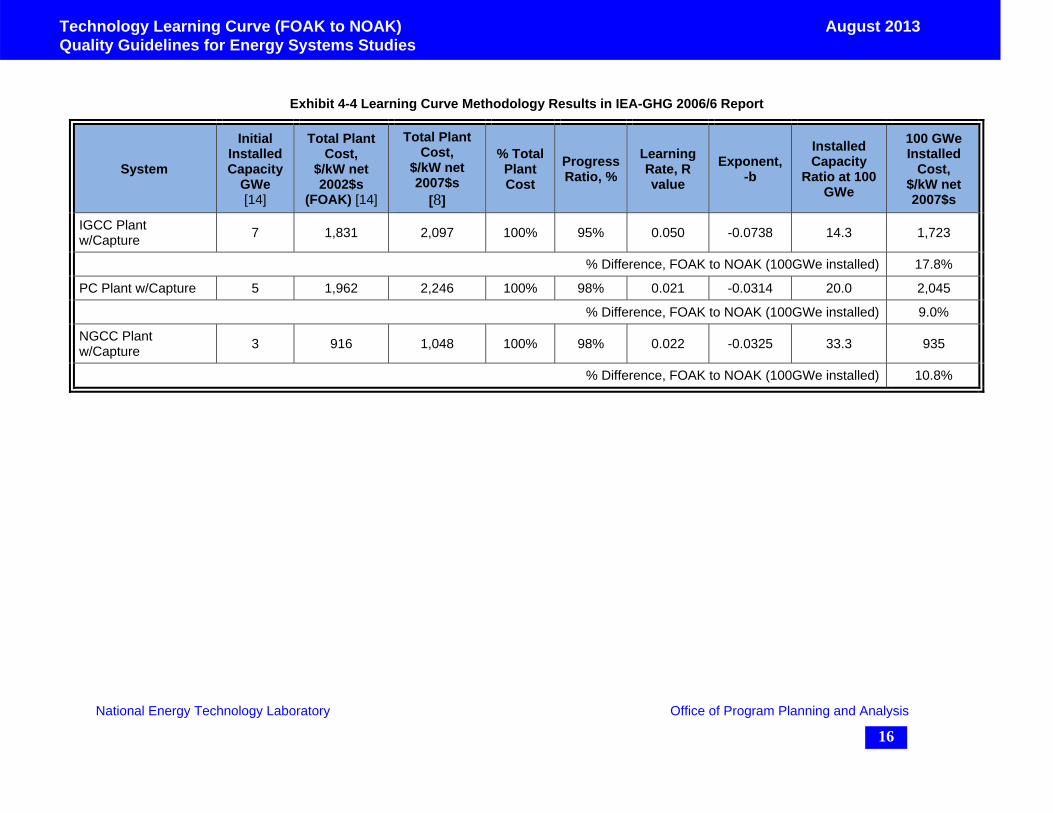
Values for similar type plants (IGCC, PC, and NGCC) from the International Energy Agency (IEA) Greenhouse Gas (GHG) Report 2006/6 [14] were converted to 2007 dollars (shown in Exhibit 4-4) and included for comparison. These values were estimated by using the installed capacity ratio (total installed capacity divided by initial installed capacity) for TPC calculations. The NOAK values were estimated at 100 GWe installed capacity. The installed capacity ratios assumed for the IEA 100 GWe estimates are significantly higher than the 5th plant assumed as NOAK in the other examples resulting in a larger percentage decrease between the FOAK and NOAK costs.

The overall TPC for the example cases are illustrated in Exhibit 4-5. The chart on the left was generated by plotting the TPC for each successive plant design (N = 1 through 33) estimated as the sum of the TPC values (TPCN=TPC1*N-b) for each account listed in Exhibit 4-1, Exhibit 4-2, and Exhibit 4-3. The chart on the right was generated by plotting the estimated TPC values from the IEA-GHG Report [14] converted to 2007 dollars (shown in Exhibit 4-4) at various installed capacity ratios (ICR = 1 through 33) where TPCR=TPC1*ICR-b. The two methodologies are compared because there are often differing opinions on whether installed capacity or number of installations better predict learning. Conceptually, the two charts are similar, with one scaling cost based on installations and the other scaling cost based on installed capacity. However, the bases are chosen such that both can be used in the same learning curve formula presented here. While there are different FOAK costs assumed in both studies, it can be seen that the trends in each of the curves are generally similar for the same power generation platforms.

The results shown here are for example purposes only. The base estimate values used in these examples are conceptual only and not intended to be definitive FOAK values. It is important to stress that learning due to research and development is not included in the scope of the learning analysis here. The FOAK plant is defined to be the first plant installed after all developmental R&D has been completed and is fundamentally the most expensive installation in the analysis timeline. FOAK costs for a specific system or plant decrease with subsequent plants due to experience gained on how to improve factors such as, but not limited to, the following: more efficient installations, startups, engineering improvements, & process streamlining.


12


August 2013

Use of this estimating procedure should be based on actual FOAK costs from historical data and not conceptually factored estimates.


13

Technology Learning Curve (FOAK to NOAK) Quality Guidelines for Energy Systems Studies

August 2013

Exhibit 4-1 Learning Curve Methodology Applied to IGCC (BB Case 4)

System Total Plant

Cost, $x1000

Total Plant Cost, $/kW net

(assumed FOAK)*

% Total Plant Cost

Progress Ratio, %

Learning Rate, R value

Exponent, -b

5th Plant Cost, $/kW net

(assumed NOAK)

Coal Handling 36,529 71 2.5% 99% 0.01 -0.0145 69

Coal Prep & Feed System 56,648 110 3.9% 98% 0.02 -0.0291 105

Feedwater/Misc. BOP 37,858 74 2.6% 96% 0.04 -0.0589 67

Gasifier & Accessories 316,648 617 21.9% 94% 0.06 -0.0893 534

ASU/Oxidant Compression 224,461 437 15.5% 94% 0.06 -0.0893 379

Gas cleanup 256,707 500 17.7% 95% 0.05 -0.0740 444

CO2 Removal/Compression 38,916 76 2.7% 97% 0.03 -0.0439 71

Combustion Turbine & Generator 132,015 257 9.1% 95% 0.05 -0.0740 228

HRSG/Ductwork/Stack 57,628 112 4.0% 99% 0.01 -0.0145 110

Steam Turbine/Generator 60,222 117 4.2% 96% 0.04 -0.0589 107

Cooling Water System 37,852 74 2.6% 99% 0.01 -0.0145 72

Ash/ Spent Sorbent Handling 37,536 73 2.6% 98% 0.02 -0.0291 70

Accessory Electric Plant 88,801 173 6.1% 99% 0.01 -0.0145 169

Instrumentation and Control 27,142 53 1.9% 99% 0.01 -0.0145 52

Site Preparation 19,796 39 1.4% 99% 0.01 -0.0145 38

Buildings and Structures 18,136 35 1.3% 99% 0.01 -0.0145 34

Total Cost 1,446,895 2,817 100% 96% 0.043 -0.0629 2,547

% Difference, FOAK to NOAK (5th plant) 9.6%

All costs in 2007$s *Costs presented in this table are conceptual values used in example calculations only and do not represent actual FOAK data.


14


August 2013

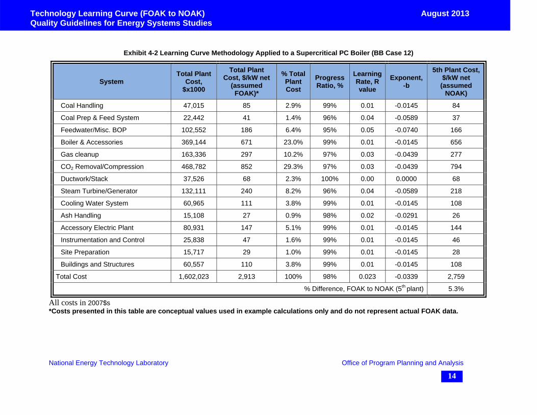
Exhibit 4-2 Learning Curve Methodology Applied to a Supercritical PC Boiler (BB Case 12)

System Total Plant

Cost, $x1000


(assumed FOAK)*

% Total Plant Cost

Progress Ratio, %


Exponent, -b


(assumed NOAK)

Coal Handling 47,015 85 2.9% 99% 0.01 -0.0145 84

Coal Prep & Feed System 22,442 41 1.4% 96% 0.04 -0.0589 37


Boiler & Accessories 369,144 671 23.0% 99% 0.01 -0.0145 656

Gas cleanup 163,336 297 10.2% 97% 0.03 -0.0439 277


Ductwork/Stack 37,526 68 2.3% 100% 0.00 0.0000 68



Ash Handling 15,108 27 0.9% 98% 0.02 -0.0291 26





Total Cost 1,602,023 2,913 100% 98% 0.023 -0.0339 2,759




15


August 2013

Exhibit 4-3 Learning Curve Methodology Applied to NGCC (BB Case 14)

System Total Plant

Cost, $x1000


(assumed FOAK)*

% Total Plant Cost

Progress Ratio, %


Exponent, -b


(assumed NOAK)



Combustion Turbine & Generator 97,490 206 16.8% 95% 0.05 -0.0740 183

HRSG/Ductwork/Stack 48,624 103 8.4% 99% 0.01 -0.0145 100







Total Cost 580,701 1,226 100.0% 97% 0.030 -0.0433 1,144




16


August 2013

Exhibit 4-4 Learning Curve Methodology Results in IEA-GHG 2006/6 Report

System

Initial Installed Capacity

GWe [14]

Total Plant Cost,

$/kW net 2002$s

(FOAK) [14]

Total Plant Cost,

$/kW net 2007$s

[8]

% Total Plant Cost

Progress Ratio, %


Exponent, -b

Installed Capacity

Ratio at 100 GWe

100 GWe Installed

Cost, $/kW net 2007$s

IGCC Plant w/Capture

7 1,831 2,097 100% 95% 0.050 -0.0738 14.3 1,723

% Difference, FOAK to NOAK (100GWe installed) 17.8%

PC Plant w/Capture 5 1,962 2,246 100% 98% 0.021 -0.0314 20.0 2,045


NGCC Plant w/Capture

3 916 1,048 100% 98% 0.022 -0.0325 33.3 935



17


August 2013

Exhibit 4-5 Example NOAK Total Plant Costs Calculated by Different Learning Curve Methodologies

Figure Source: NETL

0

500

1,000

1,500

2,000

2,500

3,000

0 5 10 15 20 25 30 35

Constant 2007 $/kW

FOAK to NOAK Plant

Total Capital Cost for Successive Plant DesignsBased on Data in NETL Bituminous Baseline Reports

BB IGCC Case 4 BB PC Case 12 BB NGCC Case 14

AssumedFOAK

5th

0

500

1,000

1,500

2,000

2,500

3,000

0 5 10 15 20 25 30 35Constant 2007 $/kW

Installed Capacity Ratio(Total Installed GW/Initial Installed GW)

Total Capital Cost at Various Installed Capacity RatiosBased on IEA‐GHG Report

IEA GHG‐8 IGCC IEA GHG‐8 PC IEA GHG‐8 NGCC

100 GWeTotal Installed

AssumedFOAK


18

August 2013 Technology Learning Curve (FOAK to NOAK) Quality Guidelines for Energy Systems Studies

5 Limitations and Caveats While learning curves have become a common tool for forecasting the costs of new energy technologies as they penetrate the marketplace, there are uncertainties involved in the use of them. For instance, the traditional learning-curve equation produces a straight line on a log-log plot; however, as mentioned earlier, the costs may increase for the first few plants in other contexts, which are just as valid as that presented here. Yeh and Rubin [19] have pointed out that no large-scale models have incorporated such cost increases, and they express concern about the modeling community’s reliance on log-linear experience curves.

Another commonly observed non-linear learning curve is one in which little or no learning occurs at the beginning, and it is not until several units have been deployed before learning begins to substantially reduce costs. Two examples are shown in Exhibit 5-1.

Exhibit 5-1. Non-Linear Learning Behavior for Power Plant Emission Control Technologies. [20]

Purchased from Elsevier [21]


19


Often this type of curve levels off over time, forming an S-shape. Yeh and Rubin [19] point out that using an S-shaped learning curve, instead of the traditional log-linear learning curve, might be more realistic, but it would give a substantially different forecast for future costs of a new technology:

Using an S-shaped EC [experience curve] for new technologies—especially environmental technologies like carbon capture and storage systems, whose deployment depends mainly on regulatory requirements—would send very different policy signals in contrast to the more “optimistic” cost reduction profiles represented by the prevailing log-linear shape. An S-shaped curve suggests that a technology could be “locked-out” of the longer-term picture if it requires a longer lead time to mature before riding down the traditional EC. In such cases, more aggressive policies such as targeted research and development (R&D) investments and early adoption incentives would be needed to alter the flat shape of the EC in its early stage. [19]

However, the difficulty with using a non-linear learning curve is that there are no non-linear learning curve equations or models available that can be used to make reliable learning forecasts.

Finally, it is important to note that learning curves were developed as an empirical measurement of learning-by-doing in manufacturing, not as a predictive tool for estimating future costs. [22]


20


6 Summary Based on the sample calculations, the proposed learning curve methodology generates reasonable predictions of NOAK plant costs from FOAK values when historical data are used to establish learning rates, capacity estimates, and FOAK cost values. The R-Values presented in this report can be used with the equations provided when detailed design information is insufficient for traditional cost estimation.

The following steps for applying the learning curve methodology are recommended and outlined in the IEA-GHG Report [14]:

Step 1: Break each plant design into major technology sub-sections

Step 2: Estimate current plant costs and contributions of each sub-section

Step 3: Select an appropriate learning rate for each sub-section/component

Step 4: Estimate the current capacity of major plant components

Step 5: Set the start of learning (FOAK) and ending (NOAK) period

Step 6: Perform a sensitivity analysis

Final values can be adjusted using more traditional economic and engineering design indices if necessary.

Users are reminded that typical techno-economic cost estimates done at NETL are conceptual feasibility studies and not definitive cost values and therefore have an associated uncertainty that is larger than the magnitude of savings due to experience. NOAK plant cost projections will have the same level of uncertainty as the FOAK plant cost estimate and, in reality, will represent a mid-point in a band of possible costs.

While valid alternate methodologies exist, NETL has elected to use this learning curve method as the way of standardizing the comparison of next-generational technologies that in some cases still have yet to be subject to a rigorous RD&D effort.


21


7 References

1 Rubin, Edward S.; Taylor, Margaret R.; Yeh, Sonia; Hounshell, David A. (2004). “Learning Curves for Environmental Technology and Their Importance for Climate Policy Analysis,” Energy (29) 1551–1559, (2004). Retrieved on April 8, 2011 from http://gsppi.berkeley.edu/faculty/mtaylor/taylor_energy29-9-10.pdf

2 Advancement of Cost Engineering (AACE) International. (2003) Conducting Technical and Economic Evaluations – as Applied for the Process and Utility Industries TCM Framework: 3.2 – Asset Planning, 3.3 – Investment Decision Making, AACE International Recommended Practice No. 16R-90, 2003. Retrieved on July 11, 2013 from http://www.aacei.org/non/rps/16R-90.pdf

3 National Energy Technology Laboratory (NETL). (2011). QGESS: Cost Estimation Methodology for NETL Assessments of Power Plant Performance, Prepared for US DOE/NETL, Pittsburgh, PA, Report No. DOE/NETL-2011/1455, April 2011, Retrieved on April 16, 2011 from http://www.netl.doe.gov/energy-analyses/pubs/QGESSNETLCostEstMethod.pdf

4 Advancement of Cost Engineering (AACE) International. (2005) Cost Estimate Classification System – As Applied in Engineering, Procurement, and Construction for the Process Industries; TCM Framework 7.3 – Cost Estimating and Budgeting, AACE International Recommended Practice No. 18R-97, 2005, Rev. November 29, 2011 Retrieved on July 11, 2013 from http://www.aacei.org/non/rps/18R-97.pdf

5 Humphreys, Kenneth and Wellman, Paul. Basic Cost Engineering, 3rd edition, Marcel Dekker, Inc., New York, pp. 10-18

6 National Energy Technology Laboratory (NETL). (2010). Cost and Performance Baseline for Fossil Energy Plants: Volume 1: Bituminous Coal and Natural Gas to Electricity, Prepared for US DOE/NETL, Pittsburgh, PA, Report No. DOE/NETL-2010/1397, Revision 2, November 2010, Retrieved on April 8, 2011 from http://www.netl.doe.gov/energy-analyses/pubs/BitBase_FinRep_Rev2.pdf

7 Electric Power Research Institute (EPRI). (2009). Technical Assessment Guide (TAG®) – Power Generation and Storage Technology Options, Electric Power Research Institute (EPRI), EPRI Product ID No. 1017465, December 12, 2009. Retrieved on April 8, 2011 from http://tag.epri.com/tag/

8 Bureau of Economic Analysis (BEA). (2011). National Economic Accounts Gross Domestic Product (GDP) U.S. Department of Commerce, Office of Management, Bureau


22


of Economic Analysis Retrieved on April 16, 2011 from http://www.bea.gov/national/index.htm#gdp

9 Chemical Engineering Plant Cost Index (CEPCI) Chemical Engineering Magazine Retrieved on April 16, 2011 from http://www.che.com/pci/

10 Department of Energy (DOE). (2004). Cost Estimate Guide for Program and Project Management, U.S. Department of Energy, Office of Management, Budget and Evaluation, April 2004 Retrieved on April 8, 2011 from http://www.emcbc.doe.gov/files/dept/CE&A/Draft%20DOE%20G%20430-1-1X_%20April%202004.pdf

11 Wright, T. (1936). “Factors Affecting the Cost of Airplanes”. Journal of Aeronautical Science Vol. 4 No. 4, pp. 122-128 (Original citing from multiple references).

12 Learning Curve Calculator, NASA Cost Estimating Website Retrieved on April 8, 2011 from http://cost.jsc.nasa.gov/learn.html

13 Learning Curve Calculator, FAS Retrieved on April 8, 2011 from http://www.fas.org/news/reference/calc/learn.htm

14 Rubin, Edward S.; Antes, Matt; Berkenpas, Michael; Yeh, Sonia. (2005). Estimating future Trends in the Cost of CO2 Capture Technologies, International Energy Agency Greenhouse Gas R&D Programme (IEA-GHG), December 2005 Retrieved on April 8, 2011 from http://steps.ucdavis.edu/People/slyeh/syeh-resources/IEA%202006-6%20Cost%20trends.pdf

15 National Energy Technology Laboratory (NETL). (2006). Nth-of-a-Kind Cost Estimation Methodology, Prepared for US DOE/NETL, Pittsburgh, PA, Final Draft Report RDS 401.01.04.004, April 2006.

16 Energy Information Administration (EIA). (2006). The Electricity Market Module of the National Energy Modeling System (NEMS) Model Documentation Report, US Energy Information Administration Report #:DOE/EIA-M068(2006), May 2009 Retrieved on April 8, 2011 from http://tonto.eia.doe.gov/ftproot/modeldoc/m068(2009).pdf

17 Energy Information Administration (EIA). (2010). Assumptions to the Annual Energy Outlook 2010 (AEO). DOE/EIA-0554(2010). Retrieved on April 8, 2011, from http://www.eia.doe.gov/oiaf/aeo/assumption/pdf/0554(2010).pdf

18 Energy Research and Investment Strategy Model (ERIS) (2006). International Institute for Applied Systems Analysis (IIASA), March 2006


23


Retrieved on April 8, 2011 from http://www.iiasa.ac.at/Research/ECS/docs/models.html#ERIS

19 Yeh, S. and Rubin, E.S. (2011). “A Review of Uncertainties in Technology Experience Curves”. Energy Economics. Prepublication version. ENEECO-02215.

20 Yeh, S.; Rubin, E.S.; Hounshell, D.A.; Taylor, M.R. (2007). “Technology Innovations and Experience Curves for NOx Control Technologies”. J. Air Waste Manage. Assoc. 55, 1827–1838.

21 Elsevier. (2012). “A Review of Uncertainties in Technology Experience Curves.” Energy Economics 34 (3) 762-771, 2012.

22 Jamasb, T. and Kohler, J. (2007). Learning Curves for Energy Technology: A Critical Assessment. Delivering a Low Carbon Energy System: Technologies, Economics and Policy, Ed: Grubb, Jamasb and Pollitt, Cambridge University Press.

technology learning curve (foak k to o noak) ) library/research/energy analysis... · an aggregate...

Documents