1

007-0217

Technological Level of Enterprises in Some Brazilian Industrial Sectors

Maria Aparecida Gouvêa

University of São Paulo, Brazil

Av. Prof. Luciano Gualberto, 908 Cidade Universitária Sala – E110

ZIP CODE 05508-900 SP

e-mail: magouvea@usp.br Phone: 55 11 30916044

Vicente Lentini Plantullo

University of São Paulo, Brazil

Av. Prof. Luciano Gualberto, 908 Cidade Universitária Sala – E110

ZIP CODE 05508-900 SP

e-mail: vplentini@uol.com.br Phone: 55 11 30916044

POMS 18th Annual Conference

Dallas, Texas, U.S.A.

May 4 to May 7, 2007

2

Abstract

The objective of this study was to verify the technological level of enterprises from different

industrial sectors in the State of São Paulo, Brazil.

A quantitative research with 165 executives from domestic and multinational companies was

conducted between July 2004 and July 2006. A list of technological techniques or tools was presented

to the interviewees for them to grade these from 1 to 7 in terms of the implementation of each one of

these aspects at their company.

The technique of factor analysis was applied and an index of technological degree was obtained, as

the weighted average of factor scores with weights that corresponded to the percentage of variance

accounted for each factor. The ensuing ranking of companies provided the relative position of each one

in terms of technological advance.

Keywords:

Technological level, Industrial sectors, Multivariate data analysis

1. INTRODUCTION

The technological level of companies reflects to what extent they have accompanied the evolution of

methods, techniques and equipment over the years in various activity sectors. The available literature

gives a most varied range of technological alternatives, although there are few texts that consider the

technological level of companies (PLANTULLO, 2006). From what we have observed the texts

pertinent technological level are not conclusive, and sometimes confused even the concept’s technical

terms. It is not uncommon to find texts that indiscriminately use, among others, terms like science,

technology, technological platform, level of software implementation and hardware. There is also the

problem that a technological advance very much above the average is expected when buying

sophisticated equipment, and without the necessary training and development of qualified

professionals.

3

In another strand we see a great number of texts linked to training and development models for

industrial company employees, which are all very interesting at the theoretical level. However,

generally speaking, they are of no practical application. A possible reason for the under-use of these

models is the concern with short and medium-term results, without evaluating the long-term nature of

the business (HENDRICKSEN, 1977).

This study was motivated to respond to the following questions:

a) What variables are most used for the technological development of industrial companies?

b) What level of technology do these industrial companies have?

c) What is the position of industrial companies on a ranking of technological development?

The central objective of this article is to present the variables that reflect the technological level of

companies, by applying statistical techniques.

In a widely globalized economy that is immersed in the digital-neural era (PLANTULLO, 2006),

knowledge of the advance of companies in the technological context and the position of each of them

relative to other companies from the same sector allows us to reflect on the competitive differential of

the ranking leaders and the need for adjustments to be made by those occupying positions in

disadvantageous conditions when it comes to strengthening themselves and facing up to the constant

challenges of the business environment.

2. THEORETICAL FOUNDATIONS

We need to explain here the differences between science and technology. Science is understood to be

acquired knowledge, although not all knowledge is considered scientific. Scientific knowledge goes

through a methodical and systematic preparation process, in such a way that its statements and

proposals may be accepted as true. Science can be understood as a set of individual pieces of scientific

knowledge, or as the systematic and ordered activity needed to obtain this knowledge. Longo (1979: 3-

4

19) defines science as “the organized set of pieces of knowledge relative to the objective universe,

involving its natural, environmental and behavioral phenomena”. For Sábato, however after Barbieri

(1983: 27), “it is the human activity, the objective of which is the search for knowledge about nature

through the application of the set of rules that constitutes the scientific method”. This said, science can

be basic (pure and/or fundamental research), or applied, according to one of the countless classification

criteria. Both use the scientific method, but in basic science or research, the search for knowledge is not

linked to practical objectives, as it is in applied science or research (RUSSELL, 1963). According to

Bunge (1980: 28), while in basic science researchers study the problems they are interested in, for

specific motives, in applied science they study problems that are of possible social interest. It is worth

highlighting that what both have in common is the fact that their objective is the search for knowledge

that might explain the reality and the methods for obtaining it. By technology we understand the

knowledge of techniques or arts, recognized as meaning skills or functions. The basic characteristic of

technology is to be essentially useful. For Schon (1967:1), technology is any tool or technique,

production or process, equipment or manufacturing method that extends human capacity. Figueiredo

(1972: 60) defines it as the “sum of pieces of knowledge of a scientific or technical nature that are

required to introduce a given industrial activity and make it function”. A more all-embracing

understanding is supplied by Longo (1979: 4): “technology is an ordered set of all the knowledge —

scientific, empirical or intuitive — used in the production and commercialization of goods and

services”. Sábato, after Barbieri (1983:5) observes that “the set of suggested pieces of knowledge that

defines a certain technology must be ordered, organized and articulated”. Technology, as “an ordered,

organized and articulated set of pieces of knowledge”, may, or may not be incorporated into the

physical or tangible goods. In the first case, implicit, or incorporated technology, this knowledge

materializes in the shape of physical capital assets and production inputs. On the other hand, in explicit,

or non-incorporated technology, the knowledge is contained in documents and people with their skills,

experiences and professional capabilities.

5

In short, the resources pertinent to the new product research and development area, articles, processes,

services and information must be sub-divided into a few items, namely: resources destined for pure and

applied research and for actual development.

The resources destined for pure research involve large sums of money and are included in what is

known as sunk costs (HENDRIKSEN, 1977); maturity times are extremely long because of the

uncertainties that exist in the environment. Pure research is a function, within research and

development (R & D) that seeks the immediate application of concepts, methodologies, philosophies

and theories developed at the global level and that must be adapted to the capitalist industrial company.

However, in the majority of industrial, commercial, service provider and information companies it still

leaves a lot to be (ROUSSEL et al., 1992).

With regard to applied research, it is necessary to spend a considerable amount of money, but the

application and maturity timescale is considerably shorter, which makes applications of an industrial

nature feasible.

With regard to the development function we need to understand that it is applied in manufacturing

process inputs, with the help of engineering, machinery and equipment maintenance, purchases and

supplies, on and off-line quality control and training and development. This function starts with small

batches being made, with a view to the final tests before its introduction in global markets (SUZAKI,

1993). Results are quantifiable in the short term and essentially practical. The relationship of this

function with the others is discrete, but very far below what is desirable for process optimization.

Various pieces of work deal with aspects linked to technology and the planning of technological

development in companies. In the light of these publications some variables were selected to reflect

the technological level of industrial companies. The variables we researched in this work with a group

of companies will be presented in the section referring to methodological aspects.

In selecting the variables relating to the technological level we focused on some of the aspects found in

the works of authors that have dedicated themselves to the theme of technology. Table 1 gives a

6

summary of the aspects and respective authors:

Table 1: Technology Aspects Aspects Authors Intelligent information technology - Q1a

Castelltort (1988), Scheer (1993), Rich and Knight (1994), Meirelles (1995), Kovács (1996), Prigogine (1996), Krajewsky and Ritzman (1999), Nussenzveig (2003) and Plantullo (2006)

Production methodologies - Q1b

Feigenbaum (1951), Goldratt and Cox (1984), Juran (1988), Osada (1989), Taguchi et al. (1990), Suzaki (1993), Deming (1990)

Finance methodologies - Q1c Kaplan and Johnson (1987) and Cogan (2006) Management philosophies - Q1d

Tomasko (1993), Hammer and Champy (1994), Morgan (1996), Santos (2005)

Level of integration - Q1e Ansoff (2001) and Hamel and Prahalad (2005) Strategic planning - Q1f

Roussel et al. (1992), Porter (2001), Ansoff (2001) and Hamel and Prahalad (2005)

3. METHODOLOGICAL ASPECTS

For the focus on variables corresponding to technological development, we arrived at the aspects

presented in Table 2 below.

7

Table 2: Names of Variables Names of the Variables

Theoretical support – Aspects of Table 1

V1. Small Group Activities (SGAs) Q1b V2. Quality Control Circles (QCCs) Q1b V3. Computer - aided Design (CAD) Q1a V4. Computer - aided Engineering (CAE) Q1a V5. Computer - aided Information Technology (CAIT) Q1a V6. Computer - aided Instruction (CAI) Q1a V7. Computer - aided Manufacturing (CAM) Q1a V8. Computer - aided Process Planning (CAPP) Q1a V9. Computer - aided Technology (CAT) Q1a V10. Computer - aided Testing (CATE) Q1a V11. Computer - integrated Manufacturing (CIM) Q1a V12. Connectivity Among Systems (CAS) Q1a V13. Statistical Quality Control (SQC) Q1b V14. Total Quality Control (TQC) Q1b V15. Activity-based Costing (ABC) Q1c V16. Downsizing (DW) Q1d V17. Integrated Process and/or Manufacturing Strategy (IPMS) Q1f V18. Integrated Information Technology Strategy (IITS) Q1f V19. Taguchi Functions (TF) Q1b V20. Activity-based Management (ABM) Q1c V21. Total Quality Management (TQM) Q1b V22. Global Sourcing (GS) Q1b V23. Just-in-Case (JIC) Q1b V24. Just-in-Time (JIT) Q1b V25. Total Productive Maintenance (TPM) Q1b V26. Organizational Change – Transversal Organizations (OC-TOs) Q1d, Q1f V27. Knowledge-network Organizations (KNOs) Q1d V28. Outplacement (OP) Q1d, Q1f V29. Reverse Strategic Planning (RSP) Q1f V30. Traditional Strategic Planning (TSP) Q1f V31. Re-engineering (RE) Q1d V32. Rightsizing (RS) Q1d, Q1f V33. Specialist Systems integrated with Artificial Intelligence

(SSIAI) Q1a

V34. Group Technology (GT) Q1b V35. Flexibility Theory (FLEXT) Q1b V36. Artificial Intelligence Theory (AIT) Q1a V37. Resilience Theory (REST) Q1b V38. Neural Networks Theory (NNT) Q1a V39. Theory of Constraints (Goldratt) (TC) Q1b V40. Chaos Theory (CHT) Q1a V41. Finite Elements Theory (FET) Q1b V42. Complex Systems Theory (CST) Q1a

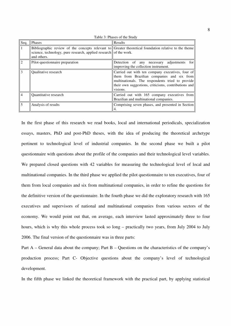
Table 3 shows the study’s planning and development phases, and the main results obtained:

8

Table 3: Phases of the Study Seq. Phases Results 1

Bibliographic review of the concepts relevant to science, technology, pure research, applied research and others.

Greater theoretical foundation relative to the theme of the work.

2 Pilot-questionnaire preparation Detection of any necessary adjustments for improving the collection instrument.

3 Qualitative research Carried out with ten company executives, four of them from Brazilian companies and six from multinationals. The respondents tried to provide their own suggestions, criticisms, contributions and visions.

4 Quantitative research Carried out with 165 company executives from Brazilian and multinational companies.

5 Analysis of results Comprising seven phases, and presented in Section 4.

In the first phase of this research we read books, local and international periodicals, specialization

essays, masters, PhD and post-PhD theses, with the idea of producing the theoretical archetype

pertinent to technological level of industrial companies. In the second phase we built a pilot

questionnaire with questions about the profile of the companies and their technological level variables.

We prepared closed questions with 42 variables for measuring the technological level of local and

multinational companies. In the third phase we applied the pilot questionnaire to ten executives, four of

them from local companies and six from multinational companies, in order to refine the questions for

the definitive version of the questionnaire. In the fourth phase we did the exploratory research with 165

executives and supervisors of national and multinational companies from various sectors of the

economy. We would point out that, on average, each interview lasted approximately three to four

hours, which is why this whole process took so long – practically two years, from July 2004 to July

2006. The final version of the questionnaire was in three parts:

Part A – General data about the company; Part B – Questions on the characteristics of the company’s

production process; Part C- Objective questions about the company’s level of technological

development.

In the fifth phase we linked the theoretical framework with the practical part, by applying statistical

9

techniques.

The population we focused on in this study is made up of companies mentioned in Exame magazine’s

Biggest and Best survey of the 500 largest companies in Brazil in the period from July 1994 to July

2006 (SANTOS; CARVALHO, 2006). We also focused on some small companies in order to obtain a

possible contrast in terms of technological performance. We researched 23 companies, each one having

more than one respondent. We interviewed 165 executives, in all. The companies researched were: 3M,

Alcoa, Bunge, Colgate-Palmolive, Daimler-Chrysler, DASA, Engemix, Festo, Galvanoplastia Mauá

Lanxess, Magneti Marelli-Cofap, Makita, Microsiga, Multibrás, Pichinin, Romi, Sanches-Blanes,

Semasa, Siemens, Sig-Simonazzi, Usimac, Votoran Cimentos and Votorantim Metais.

4. RESULTS ANALYSIS

Table 4 synthesizes the statistical techniques used and their respective objectives.

Table 4: Statistical Techniques Employed Technique Objective Frequency distribution of missing values

To find out about the distribution of each variable and decide on the variables to be maintained.

Mahalanobis’ Distance (D2) To identify outliers. Kolmogorov-Smirnov Test and asymmetry and kurtosis measures

To test univariate normality.

Descriptive statistics To obtain measures of central tendency and dispersion. Cronbach’s alpha coefficient To test the reliability of the measurement of the technological

variables’ dimension Factor analysis To find the factor scores and reduce the number of variables. Weighted average of the factor scores To measure the technological level of the companies.

4.1 MISSING VALUES ANALYSIS

The missing values frequency is generally of the order of 10%. There are some variables to eliminate

because they have a missing values rate greater than 10%, a number considered excessive in day to day

practice, although Hair et al. (2005) do not mention a particular percentage, in other words, each case

10

should be treated individually (HAIR et al., 2005: 50-51, 58-60). We eliminated the variables: V2, V15

to V16, V19 to V20, V23, V26 to V28, V33, V36 to V38 and V40 to V42. In addition, we eliminated

the variables V1, V12, V16, V24, V26 to V28 because they were not highly representative of the

Technological Level of the companies we researched, and they also had a lot of synergy with the

Essential Human Talents and Competencies (EHTC) area, the former Human Resources (HR) process.

4.2 OUTLIERS ANALYSIS

According to Hair et al. (2005: 72-73), it is necessary to check whether so-called points beyond

observation, or outliers are present, or not. This being so it is important to calculate the distance of each

observation relative to some common point. To do this we need to obtain the so-called Mahalanobis

Distance in a multidimensional space for each observation relative to the mean center of observations,

which would supply a common measure for multidimensional centrality. Hair et al. (2005) suggest a

level of 0.001, or 0.1%, to indicate an atypical observation.

The identification of outliers was done for the variables that were maintained after analysis of the

missing values.

Calculating Mahalanobis Distance (D2) relative to the number of degrees of liberty of all 23 variables,

we saw that the highest value was 2.820, with the critical value being 3.768, in other words, the highest

value is smaller than the critical value. This result proves there are no outliers in the responses,

indicating, to a certain extent, the stability of the study.

4.3 NORMALITY TEST

To test the normality of a particular variable we can use the Kolmogorov-Smirnov (K-S) Test. This test

measures the degree of concordance between the distribution of a set of sample values (observed) and a

particular theoretical distribution, thereby determining if the sample values can be reasonably

considered as coming from a population with that distribution. This test considers the following

11

hypotheses:

H0: the data come from a normally distributed population

H1: the data don’t come from a normally distributed population

We noticed that the variables do not follow a normal distribution. According to Hair et al. (2005: 76),

non-compliance with normality may be less relevant in the case of large samples. In addition, certain

statistical techniques have no normality pre-requisite for variables. Given these two provisos, the non-

normality in this study was not considered to be a concern.

4.4. DESCRIPTIVE STATISTICS

In this section we studied the main descriptive statistics of the variables maintained after analysis of the

missing values. These were: Average, Median, Mode, Standard Deviation, Variance, Variation

Coefficient, Asymmetry, Kurtosis, Range, Minimum and Maximum Value of the Variable.

Table 5 shows these statistics for the variables, using the following keys:

- AVE: Average, MD: Median, MOD: Mode, SDEV: Standard deviation, VAR: Variance, VC:

Variation coefficient, ASS: Asymmetry, KUR: Kurtosis, RAN: Range, MINV: Minimum value and

MAXV: Maximum value.

12

Table 5: Descriptive Statistics VAR AVE MD MOD SDEV VAR VC ASS KUR RAN MINV MAXV

V3 5.44 6 6 1.66 2.75 30.5 -1.35 1.10 6 1 7

V4 5.19 6 7 1.84 3.40 35.5 -0.96 -0.03 6 1 7

V5 4.79 5 7 1.90 3.60 39.7 -0.52 -0.86 6 1 7

V6 4.66 5 6 1.84 3.40 39.5 -0.48 -0.98 6 1 7

V7 5.03 6 6 1.89 3.57 37.6 -1.04 -0.07 6 1 7

V8 5.21 6 6 1.85 3.42 35.5 -1.00 -0.14 6 1 7

V9 4.73 5 6 1.84 3.38 38.9 -0.90 -0.27 6 1 7

V10 4.65 5 6 1.89 3.56 40.6 -0.70 -0.68 6 1 7

V11 4.75 6 6 2.04 4.16 42.9 -0.75 -0.78 6 1 7

V13 5.45 6 6 1.47 2.17 27.0 -1.08 0.71 6 1 7

V14 5.52 6 7 1.50 2.24 27.2 -1.03 0.63 6 1 7

V17 4.8 5 6 1.55 2.39 32.3 -0.65 -0.29 6 1 7

V18 4.92 5 6 1.62 2.63 32.9 -0.90 0.10 6 1 7

V21 5.32 6 6 1.50 2.24 28.2 -1.07 0.62 6 1 7

V22 5.11 6 6 1.69 2.86 33.1 -1.04 0.34 6 1 7

V25 5.15 5 6 1.46 2.13 28.3 -0.84 0.06 6 1 7

V29 4.33 5 6 2.01 4.05 46.4 -0.31 -1.15 6 1 7

V30 4.83 5 6 1.89 3.58 39.1 -0.67 -0.67 6 1 7

V31 4.34 4 6 1.74 3.01 40.1 -0.32 -0.80 6 1 7

V32 4.11 4 5 1.55 2.42 37.7 -0.5 -0.60 6 1 7

V34 4.23 4 4 1.78 3.18 42.1 -0.16 -0.95 6 1 7

V35 4.32 4 6 1.64 2.68 38.0 -0.29 -0.84 6 1 7

V39 3.19 3 1 2.04 4.14 63.9 0.35 -1.36 6 1 7

We need to point out that the values of the variation coefficients in percentage terms varied from 27%

(V13) to 63.9% (V39). These results are evidence that there is a myriad of different responses.

Furthermore, we saw that the variable V14 presented the greatest mean value: 5.52. On the other hand

the variables V3, V4, V7 to V8, V11, V13 to V14, V21 to V22 had the greatest median values, while

the greatest mode values were found in variables: V4 to V5 and V14.

4.5. CRONBACH’S ALPHA COEFFICIENT

According to Peter (1979), after Sobreira (2006, p. 115), the reliability of a measuring instrument is

the extent to which its measures have minimum random errors; in other words, whether an instrument

13

is capable of producing consistent results when repeated measurements are taken.

According to Hair et al. (2005, p.90), reliability is the degree by which a variable, or set of variables,

proves to be consistent with what one intends to measure. This said, to analyze reliability we used

Cronbach’s alpha coefficient, which is capable of revealing the degree to which the items of an

instrument are homogenous and reflect a certain implicit construct. According to Hair et al. (2005, p.

89-91), Cronbach’s alpha coefficient is a measure of the reliability of sample data that varies between

0.00 and 1.00, with values between 0.60 and 0.70 being considered to be the lower limit of

acceptability. This analysis will also make it possible to evaluate the sensitivity of this coefficient, by

repeatedly calculating it, excluding each aspect of the dimension and comparing the results.

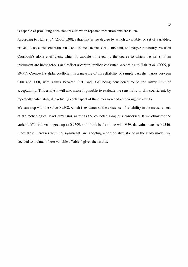
We came up with the value 0.9508, which is evidence of the existence of reliability in the measurement

of the technological level dimension as far as the collected sample is concerned. If we eliminate the

variable V34 this value goes up to 0.9509, and if this is also done with V39, the value reaches 0.9540.

Since these increases were not significant, and adopting a conservative stance in the study model, we

decided to maintain these variables. Table 6 gives the results:

14

Table 6: Cronbach’s Alpha Test Variables Scale mean if a

variable is deleted

Scale variance if an item is

deleted

Total correlation

Multiple correlation to the

square

Cronbach's alpha value if a variable is

deleted V3 105.7596 762.8446 0.7025 0.8268 0.9481 V4 105.7981 751.1530 0.7885 0.8936 0.9470 V5 106.1538 760.5975 0.6686 0.7616 0.9486 V6 106.5288 761.4943 0.6771 0.6667 0.9484 V7 106.0288 743.0380 0.8236 0.8959 0.9464 V8 105.9038 745.9907 0.7854 0.7754 0.9470 V9 106.1923 752.4093 0.7564 0.8182 0.9474

V10 106.2500 750.1893 0.8017 0.7959 0.9468 V11 106.2308 736.8394 0.8230 0.8506 0.9464 V13 105.4519 764.9103 0.8104 0.8171 0.9472 V14 105.4231 771.0426 0.7267 0.7512 0.9480 V17 106.2404 783.9902 0.5551 0.5634 0.9498 V18 106.0096 772.3397 0.6799 0.7676 0.9485 V21 105.5962 779.4081 0.6384 0.7425 0.9490 V22 105.8654 755.6516 0.7634 0.7955 0.9473 V25 105.8077 778.3316 0.6527 0.6674 0.9488 V29 106.7308 768.2375 0.5478 0.6572 0.9503 V30 106.0673 778.0634 0.5385 0.7849 0.9501 V31 106.6058 772.3771 0.6193 0.7387 0.9491 V32 106.8942 775.5324 0.6568 0.7213 0.9487 V34 106.6923 784.8753 0.4743 0.6830 0.9509 V35 106.7788 784.5040 0.4944 0.6834 0.9506 V39 108.0481 800.4928 0.2713 0.6882 0.9540

The high values of Cronbach’s coefficients signal that the variables that comprised the technological

development construct were selected appropriately.

4.6. FACTOR ANALYSIS

When working with variable data that are to be analyzed using Factor Analysis (FA), Hair et al. (2005,

p. 94) teach us that there are basic numbers for carrying out certain multivariate data analysis

techniques. This being so, in this practical case we can see that the mathematical relationship between

the number of valid observations, considering at the same time the variables maintained after analysis

of the missing values, for the total number of variables involved, is 104/23, which gives us the number

15

4.52, which is very good and close to the 5.00 required by eminent researchers. The ideal is that there

should be ten observations (HAIR et al., 2005, p. 98) per variable, but this rarely happens in practice,

above all in exploratory research, which involves obtaining primary numbers by means of interviews

with managers and directors, either from Brazilian companies or from multinational/transnational

companies.

The basic hypothesis of this technique lies in the existence of correlations between the variables, the

cause of which arises from the common factors shared between them. With this technique we analyze

the interdependence between the variables from the correlation matrix. This technique makes it

possible to capture factors that are not directly observable from the known variables taken from the

field data collected. Johnson and Wichern (1992, p. 396) explain that in common factor analysis the

variables are grouped as a function of their correlations, signifying that the variables that go to make up

a particular factor must be highly correlated between themselves and weakly correlated with the

variables that comprise the other factor.

Correlation matrix – to be pertinent the use of factor analysis it is needed to establish the existence of

significant correlations between pairs of variables, thus justifying the premiss that they do, in fact, have

factors in common.

Table 7 gives the correlations of the variables in the study.

16

Table 7: Correlations Var. V3 V4 V5 V6 V7 V8 V9 V10 V11 V13 V14 V17 V18 V21 V22 V25 V29 V30 V31 V32 V34 V35 V39

V3 1.00 0.80 0.51 0.54 0.65 0.68 0.60 0.68 0.59 0.62 0.47 0.34 0.51 0.36 0.69 0.30 0.27 0.27 0.36 0.48 0.46 0.37 0.14

V4 0.80 1.00 0.64 0.58 0.86 0.76 0.69 0.73 0.67 0.61 0.53 0.41 0.50 0.47 0.69 0.48 0.41 0.31 0.50 0.46 0.39 0.31 0.11

V5 0.51 0.64 1.00 0.64 0.67 0.56 0.71 0.62 0.68 0.64 0.55 0.39 0.50 0.37 0.43 0.38 0.53 0.30 0.48 0.29 0.15 0.17 -

0.04 V6 0.54 0.58 0.64 1.00 0.66 0.56 0.56 0.56 0.64 0.66 0.59 0.37 0.47 0.41 0.43 0.42 0.52 0.38 0.49 0.33 0.25 0.24 0.04

V7 0.65 0.86 0.67 0.66 1.00 0.77 0.79 0.74 0.73 0.66 0.57 0.44 0.45 0.57 0.60 0.48 0.41 0.36 0.43 0.53 0.42 0.41 0.22

V8 0.68 0.76 0.56 0.56 0.77 1.00 0.75 0.78 0.73 0.64 0.56 0.34 0.51 0.50 0.65 0.53 0.33 0.37 0.43 0.52 0.34 0.47 0.13

V9 0.60 0.69 0.71 0.56 0.79 0.75 1.00 0.73 0.73 0.63 0.57 0.46 0.45 0.45 0.62 0.47 0.35 0.30 0.39 0.49 0.22 0.41 0.10

V10 0.68 0.73 0.62 0.56 0.74 0.78 0.73 1.00 0.79 0.69 0.57 0.39 0.55 0.41 0.70 0.58 0.41 0.36 0.45 0.51 0.36 0.42 0.11

V11 0.59 0.67 0.68 0.64 0.73 0.73 0.73 0.79 1.00 0.63 0.54 0.51 0.59 0.34 0.59 0.56 0.49 0.37 0.57 0.57 0.40 0.50 0.22

V13 0.62 0.61 0.64 0.66 0.66 0.64 0.63 0.69 0.63 1.00 0.80 0.44 0.67 0.61 0.66 0.58 0.45 0.52 0.47 0.48 0.34 0.40 0.18

V14 0.47 0.53 0.55 0.59 0.57 0.56 0.57 0.57 0.54 0.80 1.00 0.41 0.53 0.70 0.58 0.54 0.48 0.49 0.46 0.45 0.28 0.37 0.15

V17 0.34 0.41 0.39 0.37 0.44 0.34 0.46 0.39 0.51 0.44 0.41 1.00 0.45 0.39 0.45 0.29 0.50 0.20 0.37 0.42 0.35 0.33 0.29

V18 0.51 0.50 0.50 0.47 0.45 0.51 0.45 0.55 0.59 0.67 0.53 0.45 1.00 0.45 0.65 0.54 0.43 0.56 0.61 0.45 0.21 0.36 0.03

V21 0.36 0.47 0.37 0.41 0.57 0.50 0.45 0.41 0.34 0.61 0.70 0.39 0.45 1.00 0.57 0.52 0.37 0.53 0.37 0.52 0.34 0.39 0.28

V22 0.69 0.69 0.43 0.43 0.60 0.65 0.62 0.70 0.59 0.66 0.58 0.45 0.65 0.57 1.00 0.57 0.47 0.40 0.51 0.51 0.37 0.41 0.15

V25 0.30 0.48 0.38 0.42 0.48 0.53 0.47 0.58 0.56 0.58 0.54 0.29 0.54 0.52 0.57 1.00 0.43 0.55 0.54 0.39 0.30 0.37 0.21

V29 0.27 0.41 0.53 0.52 0.41 0.33 0.35 0.41 0.49 0.45 0.48 0.50 0.43 0.37 0.47 0.43 1.00 0.38 0.63 0.24 0.24 0.10 0.06

V30 0.27 0.31 0.30 0.38 0.36 0.37 0.30 0.36 0.37 0.52 0.49 0.20 0.56 0.53 0.40 0.55 0.38 1.00 0.62 0.61 0.13 0.13 0.32

V31 0.36 0.50 0.48 0.49 0.43 0.43 0.39 0.45 0.57 0.47 0.46 0.37 0.61 0.37 0.51 0.54 0.63 0.62 1.00 0.46 0.23 0.05 0.10

V32 0.48 0.46 0.29 0.33 0.53 0.52 0.49 0.51 0.57 0.48 0.45 0.42 0.45 0.52 0.51 0.39 0.24 0.61 0.46 1.00 0.39 0.49 0.49

V34 0.46 0.39 0.15 0.25 0.42 0.34 0.22 0.36 0.40 0.34 0.28 0.35 0.21 0.34 0.37 0.30 0.24 0.13 0.23 0.39 1.00 0.52 0.63

V35 0.37 0.31 0.17 0.24 0.41 0.47 0.41 0.42 0.50 0.40 0.37 0.33 0.36 0.39 0.41 0.37 0.10 0.13 0.05 0.49 0.52 1.00 0.46

V39 0.14 0.11 -0.04 0.04 0.22 0.13 0.10 0.11 0.22 0.18 0.15 0.29 0.03 0.28 0.15 0.21 0.06 0.32 0.10 0.49 0.63 0.46 1.00

Table 7 reveals the existence of various pairs of variables with high correlation. This fact reinforces the

premiss of the existence of factors shared by the variables and the pertinence of applying factor

analysis.

Kaiser - Meyer - Olkin (KMO) Measure – this index compares the total number of correlations between

pairs of variables, with the partial correlations between them. The closer this measure is to 1, the

greater the quality of the factor analysis. KAISER (1974) classifies bands of this measure as: equal to

or greater than 0.9 – excellent; equal to, or greater than 0.8, and less than 0.9 – reliable; equal to or

greater than 0.7, and less than 0.8 – regular; equal to, or greater than 0.6, and less than 0.7 – mediocre;

equal to, or greater than 0.5, and less than 0.6 – worthless; and less than 0.5 – unacceptable.

17

Bartlett’s sphericity test – this allows the following hypothesis to be tested:

H0: the correlation matrix is an identity matrix

This hypothesis should be rejected in order to reinforce the appropriate nature of the use of factor

analysis.

Table 8 shows the KMO measure and Bartlett’s test.

Table 8: KMO Measure and Bartlett’s Test Measure of the adequacy of the sample, according to Kaiser-Meyer-Olkin (K-M-O) criteria 0.869

Approx Chi-squared. 2082.049 DF (degrees of freedom) 253

Bartlett’s sphericity test

Significance level 0.000

The KMO measure proved to be suitable. As expected the hypothesis formulated in Bartlett’s test was

rejected, thus endorsing the existence of factors underlying the variables.

Communalities – each of the original variables has an associated variance that reflects the differences

between the sample elements. The communality of each variable corresponds to the percentage of its

variance, which is accounted for the factors obtained from the factor analysis.

It is obtained by the sum of the squares of the factor loadings for each variable. The greater the value of

the communality, the more satisfactory was the substitution of a certain variable by the set of factors.

Table 9 shows the communalities we obtained. The results are satisfactory. The biggest and smallest

results relate to variables V30 and V25, respectively.

18

Eigenvalues – correspond to the total variance accounted in each factor. Eigenvalues reflect the %

variance that each factor is capable of explaining in relation to the variance of the original variables.

They allow us to establish stopping rules in accordance with their levels, in the definition of the number

of factors for the technique.

Table 9: Communalities

V3 0.688

V4 0.783

V5 0.734

V6 0.617

V7 0.798

V8 0.797

V9 0.750

V10 0.777

V11 0.765

V13 0.739

V14 0.645

V17 0.620

V18 0.620

V21 0.619

V22 0.654

V25 0.591

V29 0.785

V30 0.805

V31 0.731

V32 0.653

V34 0.733

V35 0.661

V39 0.804

19

Percentage variance accounted for each factor (before and after factor rotation) and total variance

accounted for the factors – the percentage of variance accounted for each factor is a synthesis

measurement, indicating how much of the total variance of the original variables the factor represents.

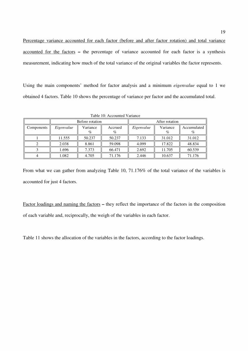
Using the main components’ method for factor analysis and a minimum eigenvalue equal to 1 we

obtained 4 factors. Table 10 shows the percentage of variance per factor and the accumulated total.

Table 10: Accounted Variance Before rotation After rotation

Components Eigenvalue Variance %

Accrued %

Eigenvalue Variance %

Accumulated %

1 11.555 50.237 50.237 7.133 31.012 31.012 2 2.038 8.861 59.098 4.099 17.822 48.834 3 1.696 7.373 66.471 2.692 11.705 60.539 4 1.082 4.705 71.176 2.446 10.637 71.176

From what we can gather from analyzing Table 10, 71.176% of the total variance of the variables is

accounted for just 4 factors.

Factor loadings and naming the factors – they reflect the importance of the factors in the composition

of each variable and, reciprocally, the weigh of the variables in each factor.

Table 11 shows the allocation of the variables in the factors, according to the factor loadings.

20

Naming the factors:

a) Intelligent Information Technology Factor (IITF), which covers the variables V3 to V11, V13 and

V22, because this factor has components that essentially have to do with computing, such as

technology, information, collection, data storage, transforming data into information and, above all,

the relationship between technology, information and telecommunications, the heart of the digital

era. It is a significant competitive differential.

Table 11: Matrix of Rotated Components

Variables Factors

1 2 3 4 V3 0.781 0.151 0.225 7.335E-02

V4 0.821 0.204 0.137 0.219

V5 0.685 0.173 -0.127 0.467

V6 0.595 0.260 -0.014 0.442

V7 0.802 0.232 0.234 0.214

V8 0.817 0.319 0.163 3.219E-02

V9 0.817 0.214 0.102 0.165

V10 0.803 0.297 0.142 0.155

V11 0.705 0.240 0.253 0.382

V13 0.615 0.545 0.125 0.219

V14 0.491 0.588 9.765E-02 0.220

V17 0.287 9.478E-02 0.402 0.606

V18 0.418 0.601 2.950E-02 0.290

V21 0.318 0.662 0.274 6.408E-02

V22 0.612 0.460 0.203 0.165

V25 0.342 0.649 0.144 0.179

V29 0.217 0.285 2.065E-02 0.811

V30 5.763E-02 0.872 9.242E-02 0.182

V31 0.222 0.560 -0.010 0.607

V32 0.325 0.536 0.508 5.196E-02

V34 0.245 2.760E-02 0.797 0.192

V35 0.400 0.172 0.670 -0.151

V39 -0.102 0.182 0.870 5.898E-02

21

b) Internal Strategic and Productive Factor (ISPF), which covers the variable V14, V18, V21, V25,

V30 and V32, because it involves the internal strategic positioning of the organization, coupled with

methods, tools and methodologies for maximizing the productivity of the machinery and equipment,

as a whole.

c) Momentary-structural Factor (MSF), which covers the variables V34, V35 and V39, in which the

need to focus on a particular problem or problems in a masterful way predominates, in addition to

modifying the structure of companies, making them lighter, more agile, in such a way as to be able

to face up to global competition.

d) External Strategic Factor (ESF), which covers the variables V17, V29 and V31, not only as far as

the traditional strategic plan, proposed by Ansoff and others, is concerned, but also reverse strategic

planning, with paradigm change, as proposed by C. K. Prahalad.

4.7. TECHNOLOGICAL LEVEL

In this section we intend to determine the technological level of industrial companies. This is a theme,

the solution of which is complex, because we have to analyze, among other considerations, the amount

of fixed assets the companies have, if the machinery and/or equipment is accompanying global

technological development, if there is a relationship between fixed assets and total capital, here

understood as being the sum of the fixed assets plus variable assets, if the company has a certain level

of product launches in the market and if it trains and develops its employees well.

To calculate the Technological Level and subsequent classification of the companies we applied the

following formula (FACHEL, 1976, p. 76-77):

22

�=

=4

1jjiji P.FI

Formula 1

where:

Ii = Global Technological Level Index, according to the ith person interviewed, i varies from 1 to

104

Fij = Factorial score for the ith person interviewed and the jth factor;

Pj = Percentage of Variance Accounted for Factor j before and after rotation, without dividing by

100.

We calculated the average of the index for each company, based on the factorial scores after rotation of

the axes using the Varimax method. The data were then standardized by dividing each average by the

maximum observed value. The maximum average obtained was 37.96, relative to Siemens.

Table 12 gives the indices of the calculated technological level for the companies we researched.

23

Table 12: Technological Level Index

3M 18.17

Alcoa 6.22

Bunge -95.30

Colgate-Palmolive 79.37

Daimler-Chrysler 43.91

Diagnósticos das Américas 44.09

Engemix -303.08

Festo -12.14

Galvanoplastia Mauá -170.07

Lanxess 0.79

Magnetti-Marelli -12.18

Makita 0.00

Microsiga -99.92

Multibrás 60.37

Pichinin 0.00

Romi 27.71

Sanches-Blanes -176.38

Siemens 100.00

Sig-Simonazzi -6.07

Usimac 58.86

Votoran - Cimentos -118.96

Votorantim Metais 0.00

As can be seen in Table 12, Siemens, Colgate-Palmolive, Multibrás, Usimac, Diagnósticos das

Américas and Daimler-Chrysler stand out as far as their technological level is concerned.

5. CONCLUSION

In the light of the theoretical point of reference presented, in this work we selected those variables in

which we were interested. Furthermore, from the results presented important information can be

highlighted:

24

a) The variables most used regarding the technological development of industrial companies, according

to the arithmetic mean, are: V14. Total Quality Control (TQC), V13. Statistical Quality Control (SQC),

V3. Computer - Aided Design (CAD), V21. Total Quality Management (TQM), V8. Computer - Aided

Process Planning (CAPP), V4. Computer - Aided Engineering (CAE), V23. Just-in-Case (JIC), V22.

Global Sourcing (GS) and V7. Computer - Aided Manufacturing (CAM).

b) From the calculations using Cronbach’s alpha coefficient, we can see that the dimension relative to

technological level is reliable, in other words, the model adapted for this study proved to be consistent

in this dimension.

The high levels of reliability reveal the consistency of the construct and that the right variables were

selected.

c) Finally, this study presented the technological level of the companies we researched and indicated

that some companies in the industrial sector are lagging behind in their actions as far as technological

development is concerned, and this aspect is extremely important in an increasingly competitive

scenario.

REFERENCES

ANSOFF, H. I.. A nova estratégia empresarial. São Paulo: Atlas, 2001.

BARBIERI, J. C.. Incentivos à produção de tecnologia no Brasil. (Dissertation submitted in the

Postgraduate Course of EAESP/FGV – Field of Concentration: Management of Production and

Industrial Operations, as a prerequisite for a Master’s Degree in Business Administration), São Paulo,

1983.

BUNGE, M.. Ciência e Desenvolvimento. Belo Horizonte, Itatiaia and São Paulo: Universidade de São

Paulo, 1980 (Coleção O Homem e A Ciência, 11).

25

CASTELLTORT, X.. CAD CAM: metodologia e aplicações práticas. São Paulo: McGraw-Hill, 1988.

COGAN, S.. Modelo de custeio baseado em atividades aplicado a decisões de produção de curto prazo.

Contabilidade Vista & Revista, v.17, p.29-46, 2006.

DEMING, W.E. Qualidade: a revolução da administração. Rio de Janeiro: Marques Saraiva, 1990.

FACHEL, J. M. G. Análise fatorial. 1976. Dissertação (Mestrado em Estatística) Instituto de

Matemática e Estatística da Universidade de São Paulo, São Paulo.

FEIGENBAUM, A. V. Quality Control. New York, USA: McGraw-Hill Book Company Inc., 1951.

FIGUEIREDO, N. F.. A transferência de tecnologia do desenvolvimento industrial do Brasil. Rio de

Janeiro: IPEA, 1972.

GOLDRATT, E. M.; COX, J.. A meta: um processo de melhoria contínua. São Paulo: Nobel, 1984.

HAIR JUNIOR, J. F.; ANDERSON, R.E.; TATHAM, R. L.; BLACK, W. C. Análise Multivariada de

Dados. 5.ed. Porto Alegre: Artmed/Bookman, 2005. 593p.

HAMEL, G.; PRAHALAD, C. K. Strategic Intent. Harvard Business Review Article, July 01, 2005.

HAMMER, M.; CHAMPY, J. Reengenharia: revolucionando a empresa em função dos clientes, da

concorrência e das grandes mudanças da gerência. 13.ed. Rio de Janeiro: Campus, 1994.

HENDRICKSEN, E. S. Accounting theory. United States: R. D. Irwin, 1977.

JOHNSON, R. A.; WICHERN, D. W. Applied multivariate statistical analysis. 3. ed. Englewood

Cliffs: Prentice Hall, 1992.

JURAN, J. M. (Editor-in-Chief), GRYNA, F. M. (Associate Editor). Juran’s quality control handbook.

4.ed. Singapore: McGraw-Hill, 1988. (Industrial Quality Series).

KAISER, H. F. An index of factorial simplicity. Psychometrika, Richmond: The Psychometric Society,

v. 39, p. 31-36, 1974.

KAPLAN, R. S.; JOHNSON, T. H. Relevance lost: the rise and fall of management accounting. USA:

Harvard School Business Press, 1987.

KOVÁCS, Z. L. Redes neurais artificiais – fundamentos e aplicações: um texto básico. São Paulo:

26

Edição Acadêmica, 1996

KRAJEWSKI, L. J.; RITZMAN, L. P. Operations Management. USA: Addison Wesley, 1999.

LONGO, W. P.. Informativo do INT . v. 3, no. 23, p.3-19. (Set./Dec. 1979)

MARRAS, J. P.. Gestão de Pessoas em empresas inovadoras. São Paulo: Futura, 2005.

MEIRELLES, F. de S. Teaching notes for the discipline of Management of Information Technology

Resources, taught as part of the master’s degree program in the São Paulo School of Business

Administration of Fundação Getulio Vargas (EASP/FGV), 1995. N.t.n.

MORGAN, G. Imagens da organização. São Paulo: Atlas, 1996.

NUSSENZVEIG, H. M. (Organização). Complexidade & caos. 2.ed. Rio de Janeiro: UFRJ/COPEA,

2003. 276p.

OSADA, T.. Housekeeping: 5’s: Seiri, Seiton, Seiso, Seiketsu, Shitsuke. Cinco pontos-chave para o

ambiente da qualidade. São Paulo: IMAM, 1989.

PLANTULLO, V. L. Um estudo empírico do grau tecnológico e dos modelos de treinamento e

desenvolvimento de empresas industriais. 2006. 346 f. Post doctoral thesis in Business Administration.

School of Economics, Business Administration and Accounting of the University of São Paulo –

FEA/USP, São Paulo.

PORTER, M.. Strategy and Internet. Harvard Business Review, 2001.

PRIGOGINE, I.. O fim das certezas: tempo, caos e as leis da natureza. São Paulo: Fundação Editora da

UNESP (FEU), 1996.

RICH, E.; KNIGHT, K.. Inteligência Artificial. 2.ed. São Paulo: Makron Books, 1994.

ROUSSEL, P.; SAAD, K. N.; BOHLIN, N. Pesquisa & Desenvolvimento: como integrar P&D ao

plano estratégico e operacional das empresas como fator de produtividade e competitividade. São

Paulo: Makron Books/Arthur D. Little, 1992.

RUSSELL, B.. Knowledge by Acquaintance and Knowledge by Description. Proceedings of the

Aristotelian Society, v. 11, pages 108-128. In: Mysticism and Logic. London: Allen and Unwin, 1963.

27

SANTOS, A. D; CARVALHO, N.. Revista Exame Melhores e Maiores: as 500 maiores empresas do

Brasil. p.58-62 e p.68-87. (Jul. 2006).

SANTOS, S. A. D. (Organizador). Empreendedorismo de base tecnológica: evolução e trajetória. 2.ed.

Maringá, Paraná: UNICORPORE Educação e comunicação corporativas, 2005.

SCHEER, A.-W.. CIM: evoluindo para a fábrica do futuro. 2.ed. Rio de Janeiro: Qualitymark, 1993

SCHON, D. A. The process of invention. In: Technology and change. New York, Seymour Lawrence

Book, Delacorte Press, 1967.

SOBREIRA NETTO, F. Medição e desempenho no gerenciamento de processos de negócios – BPM no

PNAFE: uma proposta de modelo. 2006. Tese (Doutorado em Administração) Faculdade de Economia,

Administração e Contabilidade da Universidade de São Paulo, São Paulo.

SUZAKI, K.. The new shop floor management: empowering people for continuous improvement. New

York, NY, USA: The Free Press, 1993.

TAGUCHI, G.; ELSAYED, E. A.; HSIANG, T.. Taguchi - Engenharia da Qualidade em Sistemas de

Produção. São Paulo: Mc-Graw Hill, 1990.

TOMASKO, R. M. Rethinking: repensando as corporações. Reengenharia e gestão de mudanças. São

Paulo: McGraw-Hill, 1993.