Technological Innovation, Resource

Allocation,

and Growth∗

Leonid Kogan, Dimitris Papanikolaou,

Amit Seru and Noah Stoffman

Abstract

We explore the role of technological innovation as a source of economic growth by

constructing direct measures of innovation at the firm level. We combine patent data

for US firms from 1926 to 2010 with the stock market response to news about patents

to assess the economic importance of each innovation. Our innovation measure predicts

productivity and output at the firm, industry and aggregate level. Furthermore, capital

and labor flow away from non-innovating firms towards innovating firms within an

industry. There exists a similar, though weaker, pattern across industries. Cross-

industry differences in technological innovation are strongly related to subsequent

differences in industry output growth.

JEL classifications: G14, E32, O3, O4

∗We thank Hal Varian for helping us in extracting information on Patents from Google Patents database.

We are grateful to Nick Bloom, John Cochrane, Iain Cockburn, Martin Eichenbaum, Carola Frydman, Yuriy

Gorodnichenko, John Heaton, Josh Lerner, Gustavo Manso, Petra Moser, Tom Nicholas, Stavros Panageas,

Jonathan Parker, and Monika Piazzesi for detailed comments. We also thank seminar participants at Columbia

Business School, Duke/UNC Asset Pricing Conference, International Conference, NBER Asset Pricing, NBER

Productivity, Northwestern, NYU, and SITE for helpful discussions. We are grateful to Tom Nicholas for shar-

ing his patent citations data. The authors thank the Fama-Miller Center at University of Chicago, the Zell Cen-

ter and the Jerome Kenney Fund for financial assistance. Leonid Kogan is from MIT Sloan (lkogan@mit.edu),

Dimitris Papanikolaou is from Kellogg School of Management (d-papanikolaou@kellogg.northwestern.edu),

Amit Seru is from University of Chicago (amit.seru@chicagobooth.edu) and Noah Stoffman is from Kelly

School of Business (nstoffma@indiana.edu).

Introduction

Economists since Schumpeter have argued that technological innovation combined with

resource reallocation is the driver of long-term economic growth. However, the impact of

technical change on economic growth and business cycle fluctuations remains difficult to

quantify mainly due to the scarcity of directly observable measures of innovation. Similarly,

while technology shocks play a central role in macroeconomic real business cycle models,

there is little consensus on whether the measured shocks represent actual technological

improvements, or are reduced-form representations of other economic forces.1 The primary

reason for these ambiguities is the difficulty in measuring technological innovation in the data.

This paper aims to fill this gap.

We construct a novel economic measure of innovation that combines information from

a patent dataset with stock market data over the period 1926 to 2010.2 Patents provide

useful direct information about technological innovation going as far back as the eighteenth

century. However, since patents are highly heterogeneous in their economic value, an increase

in the number of patents granted need not coincide with greater technological innovation.

Thus, constructing an empirical measure of technological innovation using patent data poses

a significant challenge.

Our central idea is to use the stock market reaction around the day each patent is granted

to appropriately weigh its information content. We interpret the stock price reaction to

patent grants using a model along the lines of Romer (1990), which models innovation as

a shock embodied in new products.3 In particular, we assume that patents are valuable

because they restrict competition among producers of new products. On the day of an

announcement of a successful patent application, the prior uncertainty about the applying

firm’s ability to extract monopoly rents going forward is resolved, resulting in the firm’s stock

price appreciation. Because patents on economically valuable new products or technologies

have higher market value, they tend to result in a larger stock market reaction. We thus use

this change in the stock market value to infer the economic value of the patent. We then

aggregate these stock market responses to patent grants to construct measures of innovation

at the firm, industry and economy level.

Our approach to measuring patent quality has several advantages over the existing

approach that relies on patent citations. While citations are informative about the intrinsic

quality of patents,4 their use as a measure of innovation is subject to two significant limitations.

1See, for instance, Cochrane (1994).2Several new studies exploit the same source of patent data (Google Patents) as we do in our paper. For

instance, see Moser and Voena (2012), Moser, Voena, and Waldinger (2012) and Lampe and Moser (2011).3Not all innovation is patentable. However, innovation that is embodied in new products is more easily

patentable (see for example Comin, 2008, for a discussion on patentable innovation). Hence, when we aremeasuring innovation through patents we are capturing technological change embodied in new products.

4See, for example, Harhoff, Narin, Scherer, and Vopel (1999), Hall, Jaffe, and Trajtenberg (2005) andMoser, Ohmstedt, and Rhode (2011).

1

First, counting the number of future citations to each patent requires information over the

entire sample. In many economic applications – such as exploring the short- and medium-run

response of investment or hiring decisions to innovation – it is desirable to use a measure

based on the contemporaneous assessment of the value of a patent, as is the case with our

measure. Second, the patent citation data is reliably available only in the later part of our

sample.5 This lack of information creates problems in assessing the quality of earlier patents,

since patents often tend to cite only the most recent ones (Caballero and Jaffe, 1993).6 In

contrast, our measure is reliably available over a long time period.

Despite these two drawbacks, patent citations provide a valuable independent measure

of the realized value of a patent. We therefore use patent citations as a validation of our

procedure. We find that the firm’s stock market reaction to the patent grant is a strong

predictor of the number of citations the patent receives in the future.

Our measure of technological innovation captures known periods of high technological

progress as well as firms participating in these waves (e.g., technologically progressive 1960s

and early 1970s, see Laitner and Stolyarov (2003)). In addition, the empirical distribution of

our firm-level innovation measure is extremely fat-tailed, since a few large firms contribute

disproportionately to the aggregate rate of innovation in the economy. The identity of these

firms varies by decade. This finding is consistent with past research describing the nature

of radical innovations (Harhoff, Scherer, and Vopel (1997)). Furthermore, we find that

characteristics of innovating firms using our measure match those of innovators as described

by Baumol (2002), Griliches (1990) and Scherer (1983).

In the second part of the paper we relate innovation to economic growth and resource

allocation. One of the benefits of our measure is that it allows us to study the relation between

innovation and subsequent changes in productivity, output and allocation of resources at

the micro level. We show that our measure of innovation is strongly related to changes in

productivity of capital and labor, both at the firm and at the industry level. Specifically, firms

and industries that innovate experience a surge in productivity and output. Furthermore, we

find that innovating firms and industries increase their use of capital and labor inputs. As a

result, we find that innovation is strongly positively related to subsequent output growth

both at the industry and firm level.

We observe several empirical patterns consistent with Schumpeter’s notion of “creative

destruction.” First, innovation activity of competing firms is negatively related to firm

productivity in the short run. Second, firms that do not innovate when their competitors do

5Moser and Nicholas (2004) and Nicholas (2008) discuss issues in extracting citations data from patentdocuments before 1975. In addition, even in the post-1975 period citation outcomes are affected by theidentity of the patent examiner (Cockburn, Kortum, and Stern, 2002).

6The first year that patent citations are officially included on patent documents is 1947. Since patentsare likely to cite only the latest patents, earlier patents will have lower citation counts. For instance, thetelephone patent by Alexander Graham Bell (patent number 174,465) has only one citation in the GooglePatent database.

2

reduce their use of capital and labor inputs. We find similar patterns of reallocation across

industries. Last, an increase in industry innovation is associated with an increase in the rate

of firm exit, consistent with the view that innovation leads to industry shakeouts.

Next, we relate our direct measure of technological change to medium-run fluctuations

in aggregate variables. We find that aggregate innovation activity is strongly positively

correlated with changes in aggregate total factor productivity (TFP) and output. In addition,

we find that aggregate consumption has a U-shaped response to the innovation shocks. This

property of our measure, and the fact that the innovation shock is associated with a decline in

the aggregate Tobin’s Q, are characteristic of embodied technology shocks (see e.g. Jovanovic

and Rousseau, 2005).

Last, we show that our measure of innovation contains additional information relative to

using the raw number of patents. We repeat our firm-level analysis measuring innovation

by the number of patent grants. The results are qualitatively similar, but the economic

magnitudes are smaller by a factor of two to three. At the aggregate level, we confirm

the findings of Shea (1999) that the relation between the number of patents and aggregate

variables is weak.

Our paper is connected to several strands of the literature. Our work is closely related to

the literature in macroeconomics that aims to measure technological innovation. Broadly, there

are three main approaches to identify technology shocks. First, researchers have measured

technological change through Solow residuals, after accounting for non-technological effects

such as imperfect competition and varying utilization (see e.g. Basu, Fernald, and Kimball,

2006). Second, researchers have imposed long-run restrictions on vector auto-regressions

(VARs) to identify technology shocks. Both of these approaches measure technology indirectly.

The resulting technology series are highly dependent on specific identification assumptions.

Our approach falls into the third category, which constructs direct measures of technological

innovation using micro data. Shea (1999) constructs direct measures of technology innovation

using patents and R&D spending and finds a weak relationship between TFP and technology

shocks. Our contrasting results suggest that this weak link is likely the result of assuming

that all patents are of equal value. Indeed, Kortum and Lerner (1998) show that there is

wide heterogeneity in the economic value of patents. Furthermore, fluctuations in the number

of patents granted are often the result of changes in patent regulation, or the quantity of

resources available to the US patent office (see e.g. Griliches, 1990; Hall and Ziedonis, 2001).

As a result, a larger number of patents does not necessarily imply greater technological

innovation. Using R&D spending to measure innovation overcomes some of these issues, but

doing so measures innovation indirectly. The link between inputs and output may vary as the

efficiency of the research sector varies over time or due to other economic forces. For instance,

Kortum (1993) documents that the patent-to-R&D ratio has shown a secular decline in the

US. The measure proposed by Alexopoulos (2011) based on books published in the field of

3

technology overcomes many of these shortcomings. However, this measure is only available

at the aggregate level, and does not directly capture the economic value of innovation. In

contrast, our measure is available at the firm level, which allows us to evaluate reallocation

and growth dynamics across firms and sectors.

Our paper is not the first to link firm patenting activity and stock market value (Pakes,

1985; Austin, 1993; Hall et al., 2005; Nicholas, 2008). In particular, Pakes (1985) examines

the relation between patents and the stock market rate of return in a sample of 120 firms

during the 1968–1975 period. His estimates imply that, on average, an unexpected arrival

of one patent is associated with an increase in the firm’s market value of $810,000. The

ultimate objective of these papers is to measure the economic value of patents; in contrast,

we use the stock market reaction as a means to an end—to construct appropriate weights

for an innovation measure which we employ to study reallocation and growth dynamics.

Our paper is also related to work that examines whether technological innovation leads to

positive knowledge spillovers or business stealing. Related to our paper is the work of Bloom,

Schankerman, and Van Reenen (2010), who disentangle the externalities generated by R&D

expenditures on firms competing in the product and technology space. We contribute to

this literature by proposing a measure of patent quality based on stock market reaction and

assessing within- as well as between-industry reallocation and growth dynamics after bursts

of innovative activity.

Our work is also related to literature on endogenous growth and creative destruction (see

Acemoglu, 2009, for a textbook treatment). We follow the spirit of the growth literature

that emphasizes the role of technological progress in promoting growth at the aggregate level

(see e.g. Aghion and Howitt, 1997) while abstracting away from the role of contracts and

inner workings of the firms in developing innovation (e.g. Gorodnichenko and Schnitzer, 2010;

Manso, 2011; Seru, 2012). Related to our work are the papers that explore the impact of

innovation on firm productivity and growth (Caballero and Jaffe, 1993; Akcigit and Kerr,

2010; Acemoglu, Akcigit, Bloom, and William, 2011). Finally, our paper is related to work

that explores the micro-foundations of aggregate economic shocks. In particular, Gabaix

(2011) proposes that if the distribution of firm size is sufficiently fat-tailed, as is the case

in the US and in most of the world, firm-specific shocks can have substantial effects on

aggregate quantities due to the failure of the law of large numbers. Consistent with this view,

the empirical distribution of firm-level innovation measure is fat-tailed, suggesting that the

innovative activity of a few large firms can have a large aggregate impact.

The remainder of the paper is organized as follows. In Section I we describe the construction

of our innovation measure. In Section II we provide external validation for our measure by

relating stock market reaction to a patent to the number of subsequent citations it receives.

Section III studies the response of individual firms and industries on our innovation measure

4

and documents patterns of reallocation. Section IV explores the response of aggregate

variables on our innovation measure. Section V concludes.

I Construction of our innovation measure

Here, we discuss the construction of our innovation measure. We start by developing a

tractable general equilibrium model that links innovative activity of a firm to its stock market

value. Using the model as a guide, we proceed to construct a measure of innovation that uses

the stock market’s response to news about patents to assess the economic importance of each

innovation.

I.A The model

We represent innovation as expanding the variety of intermediate products, borrowing several

key elements from models with endogenous growth (see e.g. Romer, 1990). To conserve space,

we relegate all derivations to the Online Appendix.

Setup

There is a competitive representative firm producing a single consumption good (numeraire)

from a variety of intermediate goods indexed by j according to the production function

Yt = Zt(LFt)1−α

∫ Ht

0

θ1−αj qαjtdj, (1)

where Zt is a disembodied productivity shock; Ht is an embodied shock representing the

current frontier state of technology; θj represents the quality of intermediate good j; qjt

represents the produced quantity of intermediate good j, whose production has a unit labor

cost; and LFt denotes the labor input used by the final-good producer. Here, note that Z

affects the productivity of all intermediate goods equally. In contrast, innovation is embodied

in new intermediate products, as it reduces the cost of producing them from infinity to one.

Hence, an increase in H only benefits the producers of the new intermediate goods. We

assume that the shocks ∆ lnZt and ∆ lnHt ≥ 0 are IID over time and independent from each

other.

There is a fixed set of firms f ∈ [0, 1] that produce intermediate goods. Each new

intermediate good created during period t is assigned a measure [(Ht −Ht−1) /χ] dj on the

interval (Ht−1, Ht]. Thus, each firm is assigned a single new intermediate good with probability

χ. If a firm receives an intermediate good, it immediately files for patent protection. The

probability that a patent is granted, pj, is itself random with an IID distribution across the

intermediate goods.

5

If the patent for good j is granted to the firm, the firm becomes a monopolist in good j

in perpetuity.7 It maximizes its intra-period profits

maxpjt

(pjt − wt) qjt (pjt) , (2)

where pjt is the spot price of good j, wt is the market wage, and qjt (pjt) is the demand

curve for good j. If the patent application for the intermediate good j is denied, all firms

have access to this innovation. In this case, the market for good j is perfectly competitive,

pjt = wt, and producing firms make zero profits from good j. After the outcome of the patent

application is decided, period-t production takes place.

Last, there is an infinitely-lived representative household that supplies a unit of labor

inelastically. The household faces a complete set of state-contingent securities and trades in

financial markets to maximize life-time utility of consumption. The household’s preferences

are

E0

[∞∑t=0

ρtc1−γt

1− γ

]. (3)

Equilibrium

If a patent for good j is granted to a firm, the firm acts as a monopolist.8 The equilibrium

level of profits from producing good j at time t equals

πjt = B3 χ−1(Hτ(j) −Hτ(j)−1

)θj ZtH

−αt , (4)

where τ(j) denotes the time good j is introduced and B3 is a constant defined in the Online

Appendix. Hence, the stock market value of the firm increases by the present value of these

profits (4), discounted using the equilibrium stochastic discount factor. Conversely, if the

patent application is declined, production of this good is competitive, hence all firms make

zero profits.

We focus on the stock market reaction to the following two information events. First,

after the market learns that firm f has applied for a patent for good j in period t, but prior

to the patent decision being made, the market value of the firm increases by

∆Vft = pj B5 χ−1 (Ht −Ht−1) θj ZtH

−αt (5)

7We could generalize the model by allowing the patent protection to expire with a constant probabilityeach period. Doing so has no qualitative impact on our results.

8There is a continuum of intermediate products in this economy, and each firm produces only a finitenumber of such products. Hence, each firm takes prices of all intermediate goods it does not produce as given.Moreover, the firm’s choice of the price for a particular good does not interact with its choices of prices forthe rest of the goods it produces. As a result, each firm chooses the spot price for each intermediate good itproduces to maximize the resulting profits, taking the demand curve for each good as given.

6

relative to the other firms.Second, if the patent application for good j is successful, the firm’s

market value increases by an additional amount

∆Vft = (1− pj) B5 χ−1 (Ht −Ht−1) θj ZtH

−αt , (6)

where B5 is a constant defined in the Online Appendix.

Aggregating the gain in market value (6) across firms with successful patent applications

in period t yields

∆Vt = B5 (1− E [pjθj]) ZtH1−αt

(1− e−∆ lnHt

). (7)

Normalizing (7) by the period-t aggregate market price Pt yields

∆VtPt

= B7 (1− E [pjθj])(1− e−∆ lnHt

)≈ B7 (1− E [pjθj]) ∆ lnHt, (8)

where the approximation is valid for small values of ∆ lnH, and B7 is a constant defined in

the Online Appendix.

The growth rate of aggregate output is determined by the disembodied shock ∆ lnZt and

changes in the frontier level of technology ∆ lnHt

∆ lnYt = (1− α) ∆ lnHt + ∆ lnZt. (9)

Discussion

The economy we consider features two aggregate shocks: the disembodied shock ∆ lnZ

and the embodied shock ∆ lnH. Our model allows us to map the stock market reaction

to successful patent grants to the innovation shock ∆ lnH.9 In the process, it provides a

number of insights.

First, the market value reaction to a successful patent application (6) is increasing in

the good-specific quality index θj and the frontier level of technology Ht. This equation

understates the total impact of the patent on the firm value because the information about

the patent allocation is known to the market before the patent application is resolved. In

particular, the total market value of a patent is given by the sum of (5) and (6).10

Second, the change in the normalized aggregate market value observed upon patent

awards (7) is increasing in the embodied technology shock ∆ lnHt. The aggregated market

9In the remainder of our analysis we will use the terms innovation and embodied shock interchangeably.To be more precise, by innovation we are explicitly referring to patentable innovation, which is embodied innew goods or processes.

10We have so far assumed that the value of the patent θj is perfectly observable to market participantsbefore the patent is granted. We show how relaxing this assumption affects our results in Section II.C.

7

reaction is informative about the average level of embodied technological progress because of

patent protection. Even though patents serve only to restrict competition and limit output,

in the absence of patent protection firms would make zero profits. Thus, the existence of

patent protection allows us to infer the value of new innovations from stock market reactions.

Third, the aggregated change in stock market value around patent grants (8) is also a

function of the contemporaneous disembodied shock ∆ lnZt. Normalizing by the end-of-period

market value (8) isolates the embodied technology shock ∆ lnHt.

Fourth, even though the firm-level market response to a successful patent grant (6)

underestimates the value of a patent θj , the effect of this bias at the aggregate level in (8) is

a constant scaling factor. Hence, the total stock market reaction across patenting firms is

increasing in the embodied shock ∆ lnH regardless of the joint distribution of pj and θj.

I.B Patents and the stock market

Our model highlights the central idea in this paper, that is, to identify the value of a patent

from the stock price reaction around the days when the market learns that a patent has been

granted to the firm. In our analysis, we use patent data from Google Patents and financial

data from CRSP. See the Online Appendix (Sections A-C) for details.

In order to examine stock market reactions, we need to define what constitutes an

information event. The USPTO’s publication, Official Gazette, which is published every

Tuesday, lists patents that are granted that day and reports details of the patent. Prior

to 2000, patent application filings were not publicized (see e.g. Austin (1993)). However,

subsequent to the American Inventors Protection Act, which became effective on November

30, 2000, the USPTO began publishing applications 18 months after filing, even if the patents

had not yet been granted. Publication of these applications occurs on Thursday of each

week. Hence, when application publication dates are available, we combine the stock market

reaction around both information events to construct our innovation measure.

To isolate market movements we focus on the firm’s idiosyncratic return, rft, defined as the

firm’s return minus the return on the market portfolio. By using this ‘market-adjusted-return

model’ (Campbell, Lo, and MacKinlay, 1997), we avoid the need to estimate the firm’s stock

market beta, therefore removing one source of measurement error. As a robustness check,

we construct the idiosyncratic return as the firm’s stock return minus the return on the

beta-matched portfolio (CRSP: bxret). This has the advantage that it relaxes the assumption

that all firms have the same amount of systematic risk, but is only available for a smaller

sample of firms. Our results are quantitatively similar when using this alternative definition.

8

Information in stock-price responses

We start by assessing if information is revealed on patent grant dates by investigating whether

stock prices behave differently on days patents are granted than when they are not. First,

in Table 1, we document that trading volume increases around the days that patents are

granted (or their applications are published). In particular, we regress a firm’s share turnover

x (trading volume divided by shares outstanding) on an announcement day dummy variable

Ifd,

xfd+k = a0 + aft + bd + b(k) Ifd + ufd, (10)

controlling for firm-year aft and day-of-week bd fixed effects. The results show that, as we vary

k from −1 to 5, there is a statistically significant increase in share turnover around the day

that the firm is granted a patent or its application is publicized. Specifically, volume increases

on the day of the announcement, and remains temporarily higher for the next two days.

We find that the total turnover in the first three days after the announcement increases by

0.16%. Given that the daily median turnover rate is 1.29%, this is an economically significant

increase in trading volume, and supports the view that patent issuance conveys important

information to the market.11 To conserve space, we report other variants of this specification

in the Online Appendix (Table 1).

Second, we find that the distribution of stock returns for patenting firms differs on days

when the firm is granted a patent relative to when the firm does not patent. In particular, we

use the subsample of patenting firms and compare the distribution of idiosyncratic returns

rft during the three day window [t, t+ 2] around patent-grant days with the distribution of

three day returns on days that no patent is granted to the firm. A Kolmogorov Smirnov test

rejects the hypothesis that the two distributions are the same at the 1 percent level.

Some illustrative case-studies

Before turning to our main results, we provide some illustrative case studies to highlight the

success of our method in identifying valuable patents. For these examples we performed an

extensive search of online and print news sources to confirm that no other news events could

account for the return around the patent dates.

The first example is patent 4,946,778, titled “Single Polypeptide Chain Binding Molecules”,

which was granted to Genex Corporation on August 7, 1990. As shown in Panel A of Figure 1,

the stock price increased 67 percent (in excess of market returns) in the three days following

the patent announcement. Investors clearly believed the patent was valuable, and news of

the patent was reported in the media. For example, on August 8 Business Wire quoted the

biotechnology head of a Washington-based patent law firm as saying “The claims issued to

11Though prices can adjust to new information absent any trading, the fact that stock turnover increasesfollowing a patent grant or publication is consistent with the view that some information is released to themarket, and not all agents share the same beliefs.

9

Genex will dominate the whole industry. Companies wishing to make, use or sell genetically

engineered SCA proteins will have to negotiate with Genex for the rights to do so.”

The patent has subsequently proved to be important on other dimensions as well. The

research that developed the patent, Bird, Hardman, Jacobson, Johnson, Kaufman, Lee, Lee,

Pope, Riordan, and Whitlow (1988), was published in Science and has since been cited over

1300 times,12 while the patent itself has been subsequently cited by 775 patents. Genex was

acquired in 1991 by another biotechnology firm, Enzon. News reports at the time indicate that

the acquisition was made in particular to give Enzon access to Genex’s protein technology.

Another example from the biotechnology industry is patent 5,585,089, granted to Protein

Design Labs on December 17, 1996. The stock rose 22 percent in the next two days on

especially high trading volume (Panel B of Figure 1). On December 20, the New York Times

reported that the patent “could affect as much as a fourth of all biotechnology drugs currently

in clinical trials.”

Finally, consider the case of patent 6,317,722 granted to Amazon.com on November 13,

2001 for the “use of electronic shopping carts to generate personal recommendations”. When

Amazon filed this patent in September 1998, online commerce was in its infancy. Amazon

alone has grown from a market capitalization of approximately $6 billion to over $100 billion

today. The importance of a patent that staked out a claim on a key part of encouraging

consumers to buy more – the now-pervasive “customers also bought” suggestions– was not

missed by investors: the stock rose 34 percent in the two days after the announcement, adding

$900 million in market capitalization (see Panel C of Figure 1).

Other patents associated with large returns include an inkjet technology granted to Canon

in 1982 (Panel D of Figure 1), and a digital storage device granted to Sperry Rand in 1959.

These examples, and a number of others we carefully investigated, indicate that our method

of identifying important patents by looking at stock returns appears to work well.

I.C Measuring innovation

We now detail the construction of our measure of innovation. We use the stock market reaction

around the day that a patent has been granted to the firm, or its application publicized, to

infer the value of each patent. Since the stock price of innovating firms may fluctuate for

reasons unrelated to innovation during the announcement window, we construct a measure of

innovation that explicitly accounts for measurement error.13 In particular, we decompose the

idiosyncratic stock return r around the time that patent j is announced as

rlj = xj + εjl, (11)

12Google Scholar citation count.13We are grateful to John Cochrane for this suggestion.

10

where xj denotes the value of patent j as a fraction of the firm’s market capitalization;

l denotes the length of the event window we use to compute returns and εjl denotes the

component of the firm’s stock return that is unrelated to the patent.

We construct the conditional expectation of the dollar value of patent j as

Aj =1

NE[xj|rljd] Sjd−1, (12)

where Sjd−1 is the market capitalization of the firm owning patent j on the day prior to the

announcement. If multiple patents N are issued to the same firm on the same day, we assign

each patent a fraction 1/N of the total value.

To recover the value of the patent, we need to make assumptions about the joint distri-

bution of x and ε. Following our model (equations (5)-(6)), the value of the patent x is a

positive random variable. Hence, we assume that x is distributed according to a Gaussian

N (0, σ2vj) truncated at zero. Further, we assume that the noise term is normally distributed,

εjl ∼ N (0, σ2ξj). Last, there is strong evidence that idiosyncratic return volatility varies

both in the time-series and the cross-section. Hence, we allow both σ2ξj and σ2

vj to vary across

firms and across time, but in constant proportions. We do this in order to reduce the number

of parameters we estimate.14

The filtered value of xj as a function of the stock return is equal to

E[xj|rlj] = δj rlj +√δj σξj

φ(Rj)

1− Φ(Rj), (13)

where φ and Φ are the standard normal pdf and cdf, respectively, and R and δ are the

normalized return and the signal-to-noise ratio respectively,

Rj = −√δj

rljσξj

, δj =σ2vj

σ2vj + σ2

ξj

. (14)

The conditional value of a patent in equation (13) is an increasing and convex function of the

daily firm return.

The next step is to choose the length of the announcement window, l. Varying the length

of the window trades off potentially omitting useful information versus potentially adding

noise to our estimates. We choose a three-day window (l = 2) and as a robustness test extend

the window to five days (l = 4).

Our assumption that σ2ξj and σ2

vj vary in constant proportions implies that the signal-to-

noise ratio is constant across firms and time, δj = δ. To estimate δ, we compute the increase

in the volatility of firm returns around patent announcement days. Specifically, we regress

14Our specification of the distribution of xj relaxes the assumption that θj is identically distributed amongintermediate goods we made in Section I.A. Doing so simplifies the empirical analysis but does not alter themain implications of the model.

11

log squared returns on a patent announcement-day dummy variable, Ifd,

ln(rlfd)2

= a0 + aft + bd + γIfd + ufd, (15)

where rlfd refers to the idiosyncratic return of firm f centered on day d with window of length

l. We control for firm-year (aft) and day-of-week (bd) fixed effects. Taking into account the

adjustment for the variance of the truncated normal, the signal-to-noise estimate can be

recovered from our estimate γ by

δ = 1−

1 +1

1−(

φ(0)1−Φ(0)

)2 (eγ − 1)

−1

. (16)

We estimate (15) using a three-day (l = 2) and a five-day (l = 4) return announcement

window. Our estimates imply δ ≈ 0.04 in both cases, so we use this as our benchmark value.15

Last, we estimate the variance of the measurement error σ2ξj. For every firm f and

year t we estimate its idiosyncratic variance, σ2ft, from daily returns. This variance is

estimated over both announcement and non-announcement days, so it is a mongrel of

both σ2v and σ2

ξ . Given the estimate of the daily variance σ2ft, the fraction of trading days

that are announcement days, µ, and our estimate γ, we recover the measurement error by

σ2ξft = σ2

ft (1 + l)(

1 + µft(1 + l) γ1−γ

)−1

.

In Table 2 we report the distribution of number of patents granted per day, idiosyncratic

firm returns rf , filtered values E[xj|rf ] and dollar values A in 1982 dollars across our sample

of 1,915,031 patents. To conserve space, we focus only on patent grant dates and a window

of 3 days. We see that distribution of firm returns is rightly skewed, and positive roughly 55

percent of the time. Our measure implies that the median value of a patent is $2.2 million,

which is comparable to the findings of Harhoff, Scherer, and Vopel (2003) and Giuri et al.

(2007) who report the distribution of valuations for small samples of European patents based

on survey responses.

Equation (13) implies that negative returns are interpreted as small values for the patent,

while positive returns are interpreted as larger positive values. This convex behavior stems

from our assumption that the value of a patent xj in equation (11) is non-negative, which

follows from equations (5)-(6) in our model. One worry is that because Aj is a convex function

of the idiosyncratic return rljd, it is influenced by the firm’s volatility. Hence, as a robustness

check, we include the firm’s idiosyncratic volatility as a control throughout our empirical

analysis. Last, to assess the benefit of explicitly recognizing the non-negativity of xj in our

estimation of the patent value, we estimate an alternative measure where we assume that

xj ∼ N (0, σ2vj), with no truncation at zero. We then follow equation (12) and construct a

15As a robustness test, we estimate equation (15) allowing the signal-to-noise ratio δ to vary across firmsize or volatility quintiles. We find no meaningful differences in the estimates of δ across quintiles.

12

second measure of patent values A, which now is equal to the total dollar change in stock

market value around the issue of patent j multiplied by our estimate of γ.

II Evidence validating our innovation measure

Prior to using our measure for empirical work, we provide evidence that it is correlated with

a measure of the realized value of a patent. In particular, we follow the literature studying

innovation that concludes that the number of times that patents are cited in the future is

correlated with the quality of the patent (Harhoff et al., 1999; Hall et al., 2005; Moser et al.,

2011). Accordingly, this section uses the number of citations a patent receives in the future

as a measure of its realized value.

II.A Patent citations

We examine whether the total number of citations the patent receives in the future Nj is

related to our innovation measure Aj using the specification

ln(1 +Nj) = a+ b ln Aj + c Zj + uj. (17)

We include a vector of controls Z that includes grant-year (or publication-year) fixed effects

because older patents have had more time to accumulate citations; the firm’s log idiosyncratic

volatility to control for its possible effect on our innovation measure; the firm’s log market

capitalization, as larger firms may produce more influential patents; the log number of patents

N granted on the same day, since it mechanically affects our measure; firm fixed effects to

control for the presence of unobservable firm effects on citations and our innovation measure;

and technology class-year fixed effects, since citation numbers may vary by industry. Since

patent applications were only publicized after 2000, we analyze the information content of

days when a patent is issued versus the firm’s application publicized separately. Initially, we

consider three-day (l = 2) announcement day windows. We cluster the standard errors by

grant or publication year and present the results with different versions of controls in Table 3.

Columns one to four of Panel I show the results of our benchmark specification – focusing

on grant dates only – with different controls. We see that our innovation measure A is

related to the number of future citations across specifications. The economic magnitudes are

substantial. The median number of citations a patent receives is 5. Our point estimates imply

that an increase from the median to the 90th percentile in terms of our innovation measure

A – corresponding to an increase of approximately 23 million 1982 US dollars – is associated

with a 9 to 54 percent proportional increase in the number of future citations.16 Columns

16Note that small changes in citations generated by a patent can be associated with large value implicationsfor the firm producing the patent. For instance, Hall et al. (2005) show that 1 more citation per patent

13

five to eight of Panel I show the corresponding estimates when we focus only on dates that

the patent application becomes public following the American Inventors Protection Act of

2000. We find that the economic magnitudes are smaller, ranging from 4 to 11 percent per

90th to 50th percentile change in A and not statistically significant if we include firm effects

in the specification.

We perform several robustness tests to our specification (17). First, we estimate a semi-log

specification, replacing log(1 + N) with N . As we see in Table 3, our point estimates are

statistically significant across specifications. An increase in A from the median to the 90th

percentile is associated with 1.3 to 6.1 (0.5 to 0.9) more citations focusing only on the

grant-day (publication day). Second, we replace log A with A. In this case, our results are

similar using patent grant days, whereas there is no consistent pattern when using publication

dates. In addition, the economic magnitudes are smaller, as an increase in A from the median

to the 90th percentile is associated with 0.2 to 0.6 more citations. Given the skewness in our

innovation measure A, we conclude that a log specification is preferable. Third, we repeat

the exercise extending the announcement window to five-days (l = 4). In this case our results

are quantitatively similar, and we provide the details in the Online Appendix (Table 5).

Last, we document the relation between our measure of the raw change in stock market

value A and the future number of citations in Table 4. Regardless of whether we use a

linear or a semi-log specification, even though the point estimates are positive, there is no

statistically significant relation between the raw change in stock market value A and the

number of citations the patent receives in the future. We interpret this finding as evidence

that the stock market reaction contains significant noise, and that our assumption that the

value of a patent is weakly positive is crucial in disentangling the information contained in

returns from components unrelated to the value of the patent.

II.B Placebo tests

Our findings in Section II.A could be influenced by unobservable, time-varying effects at the

firm level, that affect both the movements in the stock price of the firm as well as the number

of citations that patents assigned to it receives. To address this concern, we perform a series

of placebo tests to illustrate that the relation between stock market reaction to a particular

patent and the number of citations received by that patent in the future is not spurious.

In each placebo experiment, we randomly generate a different issue date for each patent

within the same year the patent is granted to the firm. We reconstruct our measure using

the placebo grant dates and estimate (17). We repeat this exercise 500 times. To conserve

space, we report the results of placebo tests corresponding only to the specification in the

first row, fourth column of Table 3.

(around the median cites per patent) is associated with 3 percent higher market value for the firm thatproduces the patent.

14

Figure 2 reports the distribution of estimate b across the placebo tests. The coefficient b

ranges from -0.01 to 0.001 across replications, substantially different from our point estimate

of 0.054. This analysis suggests that the relation between the stock market response to a

patent being granted and the number of citations the patent receives in the future is unlikely

to be spurious.

II.C Effect of imperfect information about patents

Our operating assumption so far has been that the market does not revise its beliefs about

the value of the patent at the time the patent is granted. This is because, in our model, the

information content of the patent is perfectly anticipated by the market.17 This assumption

is valid post-2000, when the American Inventors Protection Act required that patent applica-

tions be publicly available before the patent is granted. In contrast, prior to 2000, patent

applications were only disclosed to the public at the time the patent is granted to the firm.

Hence, during this period, it is possible that the market did not know the full value of the

patent prior to the patent being granted.

We now explore how the effect of imperfect information about patent quality impacts our

empirical procedure. We introduce a small modification to the model in Section I.A, allowing

for patent quality to be only imperfectly observable to the market prior to the patent being

granted. Specifically, let

s = θ + e, (18)

where e is a mean-zero random variable. The variable s is an imperfect but unbiased estimate

of patent quality that is already incorporated into the firm’s market value prior to the patent

being granted. At the time of the patent grant, the true quality of the patent θ is revealed

to the market. In this case, following a successful patent grant, the stock price of the firm

changes by

∆Vft = (1− pj) B5 χ−1 (Ht −Ht−1) θj ZtH

−αt − pj B5 χ

−1 (Ht −Ht−1)ZtH−αt ej. (19)

Examining equation (19), the stock market reaction to the patent grant contains two

components. The first part is positive, reflects the true value of the patent, and is the same

as in the baseline model. The second part is proportional to the mean-zero random variable

e that reflects the revision of market beliefs about the value of the patent.

The problem of extracting the value of the patent with imperfect information fits into

the framework of equation (11) with one modification. Specifically, the noise term ε in

equation (11) now includes movements in stock returns unrelated to the value of the patent

plus the revision in market expectations e. Hence, we might need to revisit our estimation

17Alternatively, the assumption is consistent with information about the patent being fully unanticipated.

15

of the signal-to-noise ratio δ, since we may no longer be able to use the difference in the

volatility of firm returns on patenting versus non-patenting days to infer the variance of noise.

We address this issue by assessing the nature of information about the quality of the

patent released on grant days. Specifically, we exploit the change in information disclosure

policy by the American Inventors Protection Act (AIPA) that applied to all patents filed

after November 30th. For the patents that were filed after November 30th 2000, the market

had full knowledge of their quality at the time these patents were granted. On the other

hand, for the patents filed before November 30th, it is possible that on the grant day the

stock market reaction indeed contains news about θj. We thus compare estimates of the

signal-to-noise ratio across the two sets of patents: patents that were filed just before the act,

that is in the month of November 2000; and patents that were filed immediately after the

act, that is in December 2000.

We first establish that these patents are similar in terms of quality, by comparing the

distribution of patent citations across the two groups. The Kolmogorov-Smirnov test fails

to reject the null that the two distributions are the same at the 10 percent level. Next, we

estimate the signal-to-noise ratio δ across these two sets of patents, allowing the coefficient

on the grant in equation (15) to vary across the two groups. Even though the point estimate

is 0.005 smaller for the patents filed in December 2000, the difference is not statistically

significant (p-value is 0.29). As further supporting evidence that the market was already

informed about the quality of the patents prior to the AIPA, we estimate equation (10)

separately for each group of patents, and find no evidence that the response of trading volume

on grant dates is systematically different across the two groups.

Overall, our results suggest that, prior to the enactment of AIPA, the market was as well

informed about the value of the patent before the grant date as post-2000, when the patent

document was in the public domain. These findings suggests that the variance of e may be

small and as a result we do not have to alter the estimation of the signal-to-noise ratio from

equation (11).18

III Innovation, productivity and reallocation

In this section, we study the general relation between our measure of innovation and economic

activity. We focus on the idea that resources in an economy need to be allocated to the most

productive firms and industries to maximize its overall level of production – a cornerstone of

18Nevertheless, we also investigate the robustness of our results to different values of δ. In particular,in the presence of imperfect information about the patent, equation (19) shows that our estimate of thesignal-to-noise ratio δ based on patenting versus non-patenting days might underestimate the amount ofnoise. We repeat our analysis relating patent citations to our innovation measure constructed using smallerestimates of δ (δ = 0.03 and δ = 0.015). Our results relating our measure of innovation to the number ofcitations a patent receives in the future remain very similar.

16

many models of economic growth.19 In particular, we analyze this mechanism on two broad

fronts. First, we document the link between innovation and productivity. Second, we show

that, consistent with economic optimization, productive resources flow into the innovating

firm away from firms that do not innovate.20 We perform our analysis both within and across

industries.

Before we conduct our analysis, a caveat is in order. When constructing our innovation

measure, we only use information on patents by publicly-traded firms. Hence, one worry is

that we do not include private companies, several of which might be responsible for large and

more important technology shocks.21 This omission is likely to bias our findings toward zero.

The magnitude of any bias, however, is likely to be small for two reasons. First, Bloom et al.

(2010) show that public firms in Compustat account for most of the R&D expenditures in the

United States. Second, Baumol (2002) notes that while several independent and private firms

might provide initial innovation, large publicly traded firms conduct most of the refinements

that lead to large improvements in welfare.

III.A Firm-level evidence

We start by describing how we construct our firm-level measure of innovation. We then

document the relation between our measure of innovation and capital and labor productivity,

reallocation of inputs across firms within an industry and output growth. We also discuss

these results when using other measures of innovation.

Construction of firm-level measure

We construct our dollar measure of innovation at the firm level by aggregating the dollar

values across all patents granted, or its application published (after 2000), to firm f in year t,

Avft =∑j∈P g

ft

Agj +∑j∈P p

ft

Apj , (20)

where P gft and P p

ft denote the sets of patents granted and published applications, respectively,

to firm f in year t. For most of our sample period, patent applications were kept secret until

the patent was granted, hence when constructing our firm measure we only use the stock

market reaction on the grant date. After 2000, patent applications where publicized, hence

19There exists a large literature on the importance of resource allocation for economic growth (see, e.g.Restuccia and Rogerson (2008); Hsieh and Klenow (2009); Jones (2011); Acemoglu et al. (2011)).

20Some of the economic variables we consider in this analysis are not an explicit part of our basic model.For instance, we do not introduce physical capital in our model, hence reallocation is explicitly defined onlyin terms of labor inputs. However, it is natural to consider physical capital in our empirical analysis.

21Kortum and Lerner (2000) find that venture capital, which accounts for 3 percent of total R%Dexpenditures, is responsible of 15 percent of industrial innovations.

17

following equations (5)-(6) we add the filtered dollar reaction during the patent publication

window Apj to the dollar reaction during the grant window Agj .

To avoid scale effects, we divide the dollar value of innovation Av by the end-of-year firm

market capitalization, S, in year t:

Aft =AvftSft

. (21)

Hence, our firm-level innovation measures can be interpreted as the fraction of firm f ’s value

that can be attributed to innovation in year t.

As we see in Table 5, the distribution of our firm-level measure Aft is skewed to the

right, similarly to the distribution of number of patents or patent citations at the firm level.

In addition, the distribution of our firm-level measures of innovation Af has fat tails. In

particular, restricting attention to the top 10 percent of the distribution, the relation between

the log complementary empirical cdf, log(1−F (A)), and the log innovation measure, logA is

close to linear, with a slope coefficient of −1.9 (see Figure 2 in Online Appendix). Hence, the

tail behavior of A can be well approximated by a power law.

Next, we relate our firm-level measure of innovation to firm characteristics, in particular

Tobin’s Q, firm size, K, and R&D expenditures to total assets

Aft = a0 + a1 logQt−1 + a2 logKt−1 + a3 logRDt−1 + ρAft−1 + uft. (22)

We estimate equation (22) using the entire sample of Compustat firms from 1950 to 2010

using a Tobit model.22 We include industry dummies to account for industry-level time

invariant characteristics; and time dummies to account for changing state of the business

cycle as well as changes in patent law or changes in the efficiency and resources of the USPTO

(see e.g. Griliches (1989)) during our sample period. We cluster the errors by firm.

We find that firms that are large, have higher Tobin’sQ, and have higher R&D expenditures

are more likely to innovate. These findings are similar to those discussed in Baumol (2002),

Griliches (1990), Scherer (1965) and Scherer (1983) on the characteristics of firms that have

conducted radical innovation and have been responsible for technical change in the U.S. See

the Online Appendix (Table 4) for the full set of results.

Methodology

We begin by exploring the productivity and reallocation dynamics subsequent to innovative

activity within an industry. In particular, we examine the response of productivity, Tobin’s

Q and factor demand to a firm’s own innovation activity, Af , and also to the innovation

output of its competitors. We construct our measure of innovation of a firm’s competitors,

AIf , as the average innovative activity of all firms in the same industry excluding firm f ,

22Note that information on R&D expenditure is reliably reported in Compustat only from 1975 onwards.As a result our sample period for regressions that use R&D spending is restricted to 1975–2010.

18

weighted by market capitalization S:

AIft =∑

h∈JIt\{f}

Avht

/ ∑h∈JIt\{f}

Sht, (23)

where JIt denotes the set of firms in industry I, defined according to 3-digit SIC codes.23

We explore the effect of innovation of a firm and its competitors on various firm outcome

variables, x, by estimating the regression

xft+1 = a0 + a1Aft + a2AIft + b Zft + uft+1. (24)

We include a vector of controls Z that includes lags of the dependent variable; industry fixed

effects; year fixed effects; firm idiosyncratic volatility σft to account for its possible effect on

our innovation measure; and firm and industry stock returns, to control for the possibility

that our innovation measure is inadvertently capturing changes in valuations unrelated to

innovation. In addition, we control for a number of firm characteristics that may cause the

dependent variable while being correlated with our innovation measure. Hence, we include

controls for firm size and Tobin’s Q, since large firms and growth firms innovate more; and

firm profitability, since firms experiencing a shock to profitability – for instance due to a

positive demand shock to their product – may have higher propensity to innovate. We present

results with and without these controls, and cluster the standard errors by firm.

We are interested in the estimates of a1 and a2, which capture the impact of innovation

by the firm and its competitors. A firm’s innovative output, Af , is highly skewed so we focus

on inter-decile movements in firm-level innovation to explore the economic magnitude of

a1. Our prior is that the coefficient a1 is positive, since increased innovation should have

a positive effect on firm outcomes. In contrast, the coefficient a2 can be either positive or

negative, depending on whether the innovation of other firms has a positive or a negative

effect on a firm’s outcome variables. An increase in the innovative output of competing firms

can have a positive effect on the firm because of knowledge spill-overs. However, innovation

of competitors can also have a negative effect due to business stealing or an increase in factor

prices. We should note that the presence of unobserved variables that drive the common

propensity of firms to innovate are likely to bias our estimate a2 upwards. For instance,

common productivity shocks could impact many firms in the same industry – thereby creating

a positive correlation between innovative activity of a firm’s competitors and a firm’s own

productivity.

23We obtain quantitatively similar results when we define industries according to their 4-digit SIC.

19

Productivity

First, we examine whether firms have higher productivity subsequent to innovative activity.

We consider both capital- and labor-productivity (zkft and zlft), defined as the log ratio of firm

output – total sales plus change in inventories – divided by capital or number of employees,

respectively.24 We evaluate the relation between subsequent productivity of capital and labor

and innovation by a firm Af or its competitors AI by estimating (24) with xft = [zkft, zlft].

Depending on whether we focus on the productivity of capital or labor, we measure firm size

as the stock of physical capital or number of employees respectively to ensure that our effects

are not driven by differences in the denominator of the dependent variable.

We report the results in Panel A of Table 6. We find a substantial increase in firm-

level productivity subsequent to an innovation. Our estimates of a1 imply that an increase

in innovation by the firm from the 50th to the 90th percentile leads to an 0.7% to 1.3%

increase in the productivity of capital and a 1.7% to 2.1% increase in the productivity of

labor. Furthermore, we find some evidence that the business-stealing effect dominates, as

the estimated coefficient a2 is negative and statistically significant across specifications. In

particular, a one-standard deviation increase in the amount of innovation by the firm’s

competitors is associated with a 1% to 1.7% decline in the productivity of capital and a

1.1-1.7% decline in the productivity of labor.25

Our estimates imply that the business-stealing effect is substantial. However, this finding

may be an artifact of the short horizon considered in our analysis if the business-stealing

effect and positive spillovers operate at different frequencies. In particular, positive spillovers

may affect firms with a lag, so in the medium run, the response of productivity may be

different. To explore this possibility, we estimate a dynamic version of equation (24) with

k-year ahead productivity xft+k as the regressand. We consider horizons of one to five years

k = [1..5]. To conserve space, we present results with only size, lagged productivity and

volatility controls. Including additional controls leads to quantitatively similar findings.

As we see in Figure 4, the negative effect of competitor innovation, AIf , on productivity

is stronger in the short run. As we increase the horizon k, the estimated coefficients a2(k)

increase, becoming zero or positive after 5 years. In contrast, the positive effect of firm

innovation on productivity increases with the horizon k. After 5 years, the response of

productivity of capital is between 37 to 50 percent higher than on impact. Labor productivity

displays a similar, though quantitatively stronger response. The positive effect of firm

innovation on labor productivity increases with the horizon by 65 percent.

In summary, our findings are consistent with the view that positive spillovers and business

stealing operate at different horizons. In the short run, firms that do not innovate when

24As is often the case, our measures of firm productivity may partly reflect changes in output prices.25We also explore the additional information contained in our innovation measure relative to using the

number of patents that were granted to the firm in year t; the number of citation-weighted patents; and ourraw stock market reaction A in the Online Appendix (Table 9).

20

their competitors do experience a decline in their productivity. However, in the medium

run, the innovation of other competitors has either a zero or a positive effect. This positive

effect can arise because competitor innovations affect the firm either directly, for instance

through knowledge spillovers, or indirectly, by spurring future firm innovation. Last, another

possibility, which we explore below, is that the firm scales down operations in response to

innovation by competitors and therefore operates at a higher marginal product of capital and

labor.

Tobin’s Q

Next, we explore the effect of innovation on the firm’s average Tobin’s Q. We estimate

equation (24) with xft+1 = [logQft], so that Tobin’s Q enters contemporaneously with our

innovation measure. We present the results in Panel B of Table 6.

We find that Tobin’s Q is positively related to the firm’s own innovation activity, provided

we control for its own stock return during the period. Our estimate of a1 implies that an

increase in innovation by the firm from the 50th to the 90th percentile leads to an 0.7%

increase in the firm’s Tobin’s Q. These magnitudes are in line with those reported in Hall

et al. (2005). In addition, a one standard deviation increase in the innovation activity of

other firms in the industry is associated with a 0.7% to 2.1% decline in Tobin’s Q, again

consistent with business stealing.

Reallocation

In this section we explore the reallocation dynamics subsequent to innovation by a firm. In

particular, we explore how our innovation measures are related to reallocation of physical

capital and labor. We focus on the firm’s investment and hiring rate. In addition, since

adjusting a firm’s capital and labor input often involves upfront costs, we explore the allocation

of financial resources. We focus on the net financial inflows to the firm, defined as new

issuance of equity and debt minus payouts to stock- and bond-holders.

We estimate equation (24), using firm investment, i, net hiring rate, h, and net financial

inflows, b, as outcome variables xft = [ift, hft, bft]. As before, our main estimates of interest

are a1 and a2, which capture the change in factor inputs and financial inflows following

innovation by the firm and its competitors, respectively.

In Panel A of Table 7 we examine how physical capital gets reallocated subsequent to

innovation by a firm or by its competitors. Subsequent to an innovation by a firm, there

is a substantial increase in its investment rate – defined as capital expenditures divided by

physical capital. In particular, our estimates imply that an increase in innovation by the

firm from the 50th to the 90th percentile leads to an increase in the firm’s investment rate

by 0.5% to 0.7%. This increase is statistically but also economically significant given that

the median firm investment rate is 11 percent in our sample. Furthermore, we find evidence

21

that new capital flows more towards firms that innovate than towards those that do not.

Specifically, if the firm does not innovate but its competitors do, then its investment rate is

substantially lower. A one-standard deviation increase in the level of innovation by the firm’s

competitors leads to a decline in the firm’s investment rate of 0.8-1.4%.

Next, we examine the reallocation of labor. Panel B of Table 7 shows that subsequent to

an innovation by a firm, there is a substantial increase in its employment. As before, the

economic magnitudes are significant. Our estimates imply that an increase in innovation by

the firm from the 50th to the 90th percentile leads to an increase in employment by 0.2%

to 0.5%, compared to the median firm-level hiring rate of 2.7%. In addition, labor declines

when a firm does not innovate but its competitors in the same industry do. A one-standard

deviation increase in the average innovation of the firm’s competitors leads to a reduction of

0.7% to 1.2% in the firm’s hiring rate.

Last, we examine the reallocation of net financial inflows – defined as net security issuance

minus net payout divided by book assets – subsequent to innovation by a firm. We present

the results in Panel C of Table 7. Following an innovation by a firm, there is a substantial

increase in its financial inflows. Our estimates imply that an increase in innovation by a firm

from the 50th to the 90th percentile leads to an increase of capital inflows to book assets of

0.3% to 0.6%, compared to the median level of zero capital flows. We also find that a firm is

more likely to increase payout and decrease new issuance when it does not innovate but its

competitors do. In particular, a one-standard deviation increase in the average innovation of

the firm’s competitors is associated with a reduction of up to 0.3% in net financial capital

flows to the firm, though the effect is not statistically significant across specifications.

In summary, our results in this section suggest that, consistent with economic optimization,

resources are reallocated to innovating firms and away from firms that fail to innovate when

their competitors do. In addition, we find that relative to their median value, new hiring

exhibits a quantitatively stronger response than capital, both in terms of inflow and outflow.

This increased reallocation response of labor relative to firm capital within industries is

consistent with the view that capital is more firm-specific than labor.

Output growth

The results of the previous sections imply that innovation is followed by increased productivity

of capital and labor, as well as reallocation of resources towards innovating firms. These

findings suggest that own innovation should be followed by increased output growth. In

contrast, the long-run response of output to innovation by other firms is ambiguous. It

depends on whether productivity increases in the long run, as well as whether the patterns

of reallocation we document are reversed in the long run. To answer these questions, we

estimate the dynamic response of output – measured as firm sales plus change in inventories –

22

to the firm’s own innovation Af and innovation by its competitors AIf

log yft+k = a0 + a1Aft + a2AIft + b Zft + uft+k. (25)

Our vector of controls includes firm and industry stock returns; firm idiosyncratic volatility;

firm size (capital); two lags of the dependent variable; industry and time fixed effects. We

cluster the standard errors by firm. We again examine horizons of k = 1 to k = 5 years. We

plot the estimated coefficients a1(k) and a2(k) in Panels (a) and (b) of Figure 5, along with

90 percent confidence intervals.

We find that firm output displays a positive and statistically significant response to an

own-innovation shock. A firm that experiences an innovation shock from the median to the

90th percentile experiences a 1.5% increase in output over a period of 5 years. In contrast, a

positive one-standard-deviation shock to innovation by other firms in the same industry is

associated with a decline in output by 2.5% to 3.5%. Here, we should note that since we do

not have access to firm-level price data, we cannot distinguish an increase in market share

from an increase in the quantity of output.

Comparison to other measures

Here, we explore the additional information contained in our innovation measure relative

to using the number of patents that were granted to the firm in year t; the number of

citation-weighted patents; and our raw stock market reaction A. For brevity, we summarize

the results here and refer the reader to the Online Appendix (Tables 6-8) for more details.

First, we measure innovation Aft as the number of patents granted to firm f in year t,

and construct AIft as the average number of patents granted to the firm’s competitors in

the same year. We estimate equation (24) for capital and labor productivity; investment;

labor hiring; and financial flows. We find qualitatively similar results as our innovation

measure, but the magnitudes are smaller by a factor of 2 to 3. Second, we repeat the same

exercise replacing patent counts with citation-weighted counts. In contrast to our measure,

citations contain information not available to economic actors at the time that production

and allocation decisions are made. In this case, our results are qualitatively similar, slightly

stronger than using patents alone but smaller in magnitude by a factor of 2 compared to

our benchmark measure. Third, we repeat this exercise using the raw stock market reaction

A. In this case our results are mostly qualitatively similar, though not always statistically

significant across specifications. Furthermore, the economic magnitudes are smaller than our

baseline results by a factor of 5. This provides further evidence that the raw stock market

reaction contains significant noise and that our identification assumption in equation (11)

– that the value of a patent x is positive – improves upon the raw measure by parsing out

information contained in returns that are unrelated to the value of the patent.

23

III.B Industry-level evidence

So far we have focused on the dynamics of productivity and reallocation within an industry.

We now conduct a similar exercise examining the response of productivity and reallocation of

inputs at the sector level. To do so, we use the KLEMS industry-level output data provided by

Dale Jorgenson. First, we document the dynamic response of capital and labor productivity,

defined as the ratio of the quantity of output to the quantity of capital and labor services,

respectively. Second, we focus on the reallocation of inputs, namely the growth rate in the

quantity of capital and labor services. Last, we relate the rate of establishment exit to our

innovation measures, using information on establishment exit rates at the industry level from

the US Census tables on Business Dynamics Statistics (BDS).

Construction of industry measures of innovation

We construct industry-level measures of innovation by aggregating our firm-level dollar

measures of innovation across the set JIt of firms in industry I

AvIt =∑f∈JIt

Avft. (26)

Our dollar measure Av will be mechanically affected by economic forces that affect the level

of stock prices but are likely to be unrelated to innovation, such as disembodied productivity

shocks or changes in discount rates. Hence, following equation (8), we scale our dollar measure

AvI by the total market capitalization of the industry SI

AIt =AvItSIt

, (27)

where St =∑

f∈JIt Sft. Thus, our industry-level measure, AIt, is the value-weighted average

of our firm-level innovation measure Aft across all firms in the industry.

Methodology

We estimate specifications similar to (24), but at the industry level:

xIt+1 = a0 + a1AIt + a2AMIt + b Zt + uIt+1. (28)

Here, AI is our measure of innovation at the industry, and AMI is the average level of

innovation in the economy, excluding industry I constructed in a manner similar to (23).

In analogy to the firm-level regressions, we include a vector of controls Z which includes:

industry stock returns; the average idiosyncratic volatility in the industry; time effects; and

lagged values of the dependent variable. In the presence of time dummies, the interpretation

24

of the coefficient a2 is unclear, so we only include one of the two. We cluster the standard

errors by industry.

Productivity

First, we explore the dynamic response of industry productivity to its own innovation AI and

the innovation of the other industries AMI . We are interested in the coefficients a1 and a2,

which measure the response of productivity to an industry and economy-wide (excluding the

given industry) innovation shock respectively. The coefficient a1 is informative as to whether

innovation creates net value or is a zero-sum game that merely affects the distribution of rents

within an industry. We estimate (28) with k-period ahead productivity as the regressand,

xft+1 = [log zkft+k, log zlft+k]. We consider horizons of one to five years k = [1..5]. We plot the

results in Figure 6, controlling for lagged productivity and volatility. Controlling for firm- or

industry-level stock returns leads to similar results.

We find that both labor and capital productivity increase in response to own industry

innovation. A one-standard-deviation AI shock is associated with a 2.5% increase in the

productivity of capital and labor, after a period of 5 years. By contrast, capital and labor

productivity show no statistically significant response to the innovation activity of other

industries.

Reallocation and creative destruction

Next, we examine the response of capital and labor to an industry innovation shock, as well

as to the innovation of other industries. We estimate equation (28), using as the outcome

variable the growth rate in the quantity of capital and labor services xIt = [iIt, hIt]. As before,

the main estimates of interest in this specification are a1 and a2, which capture the change in

the quantity of factor inputs in response to innovation in the industry and the rest of the

economy respectively. We show our results in Table 8.

We find that an increase in the amount of industry innovation increases the quantity of

capital and labor services used by the industry, though in some specifications the effect is not

statistically different from zero. As before, we find that the response of labor is greater than

the response of capital. An increase in industry innovation is associated with a 0.2% to 0.4%

increase in capital services and a 0.3% to 0.7% increase in labor services. These magnitudes

are economically significant, given that the median annual growth rate in capital and labor

services equals 3.1% and 0.7% respectively.

Our results suggest that increases in economy-wide innovation lead to cross-industry

reallocation of labor and capital. In particular, a one-standard-deviation increase in the

economy-wide innovation measure is associated with a 0.5% to 1.0% decline in the growth of

capital services and a 1.4% to 2.2% decline in the growth of labor services.

25

Next, we examine patterns of firm turnover at the industry level. Our measure captures

the innovation of existing firms, since we do not observe the firm’s innovation activity prior

to entry. Hence, we relate firm exit to innovation by incumbent firms. If industry innovation

spurs creative destruction, we expect to find a positive relation between the rate of firm

exit and the level of industry innovation. We estimate specifications similar to (28), but we

replace the outcome variable with the rate of firm exit and examine the response of this

variable to own industry innovation AI and innovation of other industries AMI . Table 9

presents the results.

Industry innovation is accompanied by an increase in firm exit. The estimated coefficient

a1 is positive and statistically significant across specifications. Innovation accounts for an

economically significant fraction of the variation in firm exit rates. A one standard deviation

increase in industry innovation is associated with an increase in the firm exit rate by 0.2%

to 0.4%, while the unconditional volatility of exit rates is equal to 2.1%. Economy-wide

innovation AMI has no statistically significant effect on firm exit.

Output growth

Last, we explore the dynamic response of the quantity of industry output to industry

innovation AI and innovation of other industries AIM , by estimating a specification similar

to (25)

log yIt+k = a0 + a1AIt + a2AMIt + b ZIt + uIt+k, (29)

where our vector of controls Z includes industry stock returns; the cross-sectional average

idiosyncratic volatility; and two lags of the dependent variable. We again examine horizons

of k = 1 to k = 5 years. We plot the estimated coefficients a1(k) and a2(k) in Panels (c) and

(d) of Figure 7, along with 90 percent confidence intervals.

Innovation is associated with substantial subsequent increases in output. In particular,

the response of output at the industry level is qualitatively similar to the firm-level responses,

though the magnitudes are stronger. A one standard deviation shock to industry innovation

is associated with a 5 percent output growth over a period of 5 years. In contrast, a positive

innovation by other industries, is associated with a 3.5% to 6.8% decline in output. In

contrast to our firm-level output results, industry output is deflated by price, hence our

results correspond to real increases in output rather than market share.

The results of this section can be summarized by examining the relation between industry

innovation in the first half of the sample (1960–1982) and subsequent output growth in the

second half of the sample (1983–2006). In Figure 8 we plot the industry innovation measure

AI averaged over the first half of the sample (1960–1982) on the X axis and the corresponding

output growth of the industry in the second half of the sample (1983–2006) on the Y axis.

26

The correlation between the two series is 41 percent with a robust t-statistic of 2.6. Industries

which experienced high technological innovation in the first half of the sample were also

the ones whose growth rate was subsequently higher in the second half of the sample. For

example, industries such as Electrical Machinery, Automotive and Communication, which are

in the highest quartile of innovation during the first half of the sample, had an annualized

growth rate of more than 4 percent over the second part of the sample. Similar correlation is

found for low-innovative industries such as Textile and Utilities.26

IV Innovation and aggregate dynamics

Our results in the previous section show that innovation is positively related to subsequent

changes in industry-level productivity and output growth, especially in the medium term. In

this section, we analyze the effect of innovation at the level of the U.S. economy.

IV.A Construction of aggregate measures of innovation

We construct economy-wide measures of innovation by aggregating our firm-level measure

across the set Jt of firms across the entire economy

Avt =∑f∈Jt

Avft. (30)

As before, we scale our dollar measure Av by the total market capitalization

At =AvtSt, (31)

where St =∑

f∈Jt Sft is the total market capitalization of all firms in our sample.

Examining the composition of our aggregate innovation measure A, we find that a few

large firms account for a significant fraction of the aggregate rate of innovation in the economy.

The identity of these firms varies by decade. In the 1930s and 1940s, AT&T and GM are

responsible for a large share of innovative activity. In the 1950s and 1960s, du Pont and Kodak

take a leading role. In 1970s and 1980s, a large share of innovation takes place in Exxon, GE,

3M and IBM. Finally, in the 1990s and 2000s, “new economy” firms are responsible for a

large share of innovation, namely Sun, Oracle, Microsoft, Intel, Cisco, Dell, and Apple.

26One source of concern with our analysis could be that the relation between innovation and output growthis driven by omitted variables. To alleviate these concerns we generate exogenous changes in R&D activityacross industries by employing the Bloom et al. (2010) instrument for firm-level R&D activity. As discussedin Bloom et al. (2010), the firm-level tax price of R&D can be decomposed into a component that is relativelyexogenous since it is based solely on federal rules. In unreported tests we use the Bloom et al. (2010) firm-levelR&D instrument and construct its industry counterpart by taking the average of this tax price across firmsin a given industry. We find qualitatively similar results to those reported in the table when we instrumentthe endogenous innovation variable (A).

27

We compare our measure of aggregate innovation with three aggregate measures proposed

in the literature: the log number of total patents granted; the log R&D expenditures from

the BEA; and the log number of technology books published from Alexopoulos (2011). Some

of these measures show a secular time trend, so we remove a deterministic time-trend from

all measures. We plot these series in Figure 3.

Our measure of innovative activity lines up well with the three major waves of technological

innovation in the U.S. First, our measure suggests high values of technological innovation in

the 1930s, consistent with the views expressed in Field (2003). When we dissect our measures

we find that firms that primarily contribute to technological developments during the thirties

are in the automobiles (such as General Motors) and telecommunication (such as AT&T)

sectors. This description is consistent with studies that have examined which sectors and

firms led to technological developments and progress in the 1930s (Smiley, 1994).

Second, our measure suggests higher innovative activity during 1960s and early 1970s –

a period commonly recognized as a period of high innovation in the U.S (see Laitner and

Stolyarov (2003)). As has been noted, this was a period that saw development in chemicals,

oil and computing/electronics – the same sectors we find to be contributing the most to our

measure with major innovators being firms such as IBM, GE, 3M, Exxon, Eastman Kodak,

du Pont and Xerox.

Third, developments in computing and telecommunication have brought about the lat-

est wave of technological progress in the 1990s and 2000s, which coincides with the high

values of our measure. In particular, it is argued that this is a period when innovations

in telecommunications and computer networking spawned a vast computer hardware and

software industry and revolutionized the way many industries operate. We find that firms

that are main contributors to our measure belong to these sectors with firms such as Sun

Microsystems, Oracle, EMC, Dell, Intel, IBM, AT&T, Cisco, Microsoft and Apple being

the leaders of the pack. We next turn to providing firm level evidence that lends additional

support to validity of our measures.

Comparing the aggregate innovation series, we note three important points. First, our

measure displays different behavior than the total number of patents, especially in the

beginning and towards the end of the sample. The correlation between At and the log number

of patents is equal to 0.42 in levels and 0.11 in first differences. Second, our innovation

measure captures similar low-frequency movements to R&D spending and the number of

technology books published in the Library of Congress, in particular the rise in innovative

activity during the 1960s and early 1970s. Finally, our innovation measure displays substantial

high-frequency variability relative to either the stock of R&D or the number of technology

books. Some of this variability comes from variation in the number of patents granted, but a

significant part comes from changes in the average response of the stock market on these

28

patent grant dates. In contrast, the stock of R&D capital and the number of technology

books display mostly low-frequency variation.

IV.B Evidence

In this section, we examine the extent to which our innovation measures account for short-

and medium-run fluctuations in aggregate economic quantities. We start by exploring the

relation between measures of innovation and quantities of interest using VARs and VECMs.

Then, we explore whether our results are sensitive to the details of the specification.

Methodology

We estimate bivariate VARs of the form Z = [logX, logA]′, where X is our variable of

interest and A is our measure of innovation. In addition, we also compute responses using

a vector-error-correction model (VECM), including a deterministic trend. The number of

cointegrating relations are selected using the Johansen test, which suggests the presence

of one cointegrating relation in all systems. The number of lags are selected using the

Akaike-Information Criterion, which advocates a lag length of one to two years for each of

the systems. We plot the impulse-response functions in Figures 9 and 10, along with 90

percent confidence intervals. Standard errors are computed by a bootstrap simulation of 500

samples. The impulse responses are computed by ordering the innovation shock A last, so

the technology shock affects the variables of interest only with a lag.

Total Factor Productivity and Output

First, we focus on aggregate productivity and output, with productivity measured using

utilization-adjusted TFP from Basu et al. (2006) and output measured as the real per capita

gross domestic product. We find that TFP increases by 1 to 2 percent over 8 years following

a one-standard deviation increase in innovation output, depending on whether we use the

VAR or the VECM specification. The forecast error variance attributed to our innovation

measure ranges from 36 to 70 percent at the 8-year horizon, depending on the specification.

Our findings are comparable to the results in Alexopoulos (2011), but in contrast to Shea

(1999) who uses only information on patents and finds a negative relation.

Aggregate output displays a delayed positive response. In the first two years, the response

of output to a one-standard deviation shock is slightly negative at -0.2% but statistically

insignificant. However, output increases in the long run by a substantial amount: a one-

standard deviation innovation shock results in a net 2.5% to 4.2% increase in aggregate

output after 8 years. The share of 8-year forecast-error variance attributed to our innovation

measure ranges from 5 to 13 percent .

29

We perform several robustness tests. For brevity, we summarize the results here and

refer the reader to the Online Appendix for the full set of results. First, we include the

cross-sectional average of idiosyncratic volatility σ to ensure that our innovation measure

does not pick up movements in firm-level volatility. We order volatility second, so now

Z = [logX, log σ, logA]′. The magnitudes of the impulse responses are similar in this

specification (see Figure 3 in the Online Appendix).

Second, we explore whether our measure of innovation contains incremental information to

stock prices. Following Beaudry and Portier (2006), we include the level of the stock market

in our VAR, scaled by the consumption deflator and population.27 This helps us evaluate the

extent to which our results are driven by variation in the denominator of A (the stock market

capitalization). We order the level of stock prices second, so now Z = [logX, logM, logA]′.

Our results are qualitatively similar in terms of statistical significance, but the economic

magnitudes are somewhat smaller for TFP (see Figure 4 in the Online Appendix). Productivity

and output increase by 0.5 and 2.6% respectively at the peak following a one-standard

deviation shock in our technological innovation measure. In contrast, the response of output

to a one-standard deviation shock in logM is not statistically significant beyond the one-year

horizon. Furthermore, the innovation shock accounts for a comparable fraction of the variance

of productivity (13.9%) and output (10.5%) relative to the stock market shock (13.4% and

4%, respectively). Hence, our innovation shock contains incremental information about future

productivity and output to the level of the stock market.

Last, we repeat the analysis using k-period OLS regressions of T -period ahead growth

rates of output and TFP on first differences in our innovation measure. Doing so verifies that

our findings are not driven by specification of the VAR/VECM. We find similar results: an

increase in innovation has a permanent positive effect on the level of TFP. In the short run,

output exhibits slightly negative response, and it increases in the long run (see Table 10 in

the Online Appendix).

Comparison to number of patents and R&D spending

We also explore whether our measure of innovation contributes information relative to other

commonly employed measures of technological innovation: R&D spending, and the log number

of patents. We estimate bivariate VARs for productivity and output, with the log number

of patents or R&D spending series ordered last. The number of patents has some ability to

predict TFP, but the results are quantitatively weaker. A one-standard deviation shock to

the log number of patents is associated with a 0.4% increase in TFP, and the patent shock

accounts for 13.1% of the forecast error variance. Output shows no statistically significant

response to number of patents. In contrast, R&D Expenditure has some ability to predict

27We depart from Beaudry and Portier (2006) in that we include the level of the CRSP value-weightedrather the level of the S&P 500 index, since the former includes all stocks traded on the three major exchanges.

30

output, but not productivity. Output drops in the short run by 0.4%. At the eight-year

horizon output displays a statistically significant increase of 0.3%.28

Consumption

Next, we analyze the impulse response of aggregate consumption to our innovation measure.

The response of consumption is informative about whether our innovation measure is an

example of an embodied or disembodied shock. If technological innovation represents a

disembodied shock, we expect that consumption should increase immediately. Due to the

positive wealth effect, agents anticipating an increase in future consumption would like to

increase their consumption today. In contrast, if innovation is embodied in new vintages of

capital, then consumption may only increase in the long run. In the short run, agents will

divert resources away from consumption towards adopting new innovations.

We analyze the response of real per capita consumption of non-durables and services using

VARs and VECMs, as in Section IV.B. We plot the impulse-response functions in Figure 11,

along with 90 percent confidence intervals. We find that consumption displays a U-shaped

response to innovation. In the first two years consumption displays a statistically significant

drop of 0.5% to 0.6%. Subsequently, consumption increases, leading to a 0.3% to 0.6% net

increase after 8 years. The innovation shock accounts for 5 to 7 percent of the forecast-error

variance of consumption growth after 8 years.

The short-run decline in consumption is consistent with the delayed response of output in

Section IV.B. Innovation affects output with a lag, so the positive response of consumption is

necessarily delayed. This evidence suggests that our innovation measure at least partially

captures an embodied – rather than a disembodied – technology shock.

Innovation and Tobin’s Q

We conclude our analysis by examining the relationship between our measures of innovation

and Tobin’s Q at the aggregate level. The theoretical relation between innovation and Tobin’s

Q is ambiguous. If innovation represents an increase in TFP that costlessly affects all firms

– a disembodied shock – then standard models will imply that average Tobin’s Q should

rise (see, e.g. Hayashi (1982)). However, it is also possible that innovation renders part of

the capital stock obsolete (see e.g. Laitner and Stolyarov (2003)) or a reduction in profits

for incumbent firms (e.g. Greenwood and Jovanovic (1999); Hobijn and Jovanovic (2001);

Garleanu, Kogan, and Panageas (2012)). In these cases technological innovation represents

28We also explore if our measure of innovation is predictable by output or productivity. If the measurecaptures fundamental shocks we expect to find limited evidence of predictability. In addition, we explorewhether our measure of innovation is predictable by other measures of technological growth in the literature,for instance the book-based measures of Alexopoulos (2011) and the stock of R&D capital. In unreportedtests we find that output and TFP do not Granger-cause our measure of innovation. Further, our measure ofinnovation is distinct from the measures of Alexopoulos (2011), in that neither causes the other. Finally, ourmeasure is also not Granger-caused by either the number of patents or R&D spending.

31

an embodied shock, and thus the relationship between innovation and average Tobin’s Q

could be negative.

We estimate the contemporaneous response of Tobin’s Q to our innovation measures

∆ logQt = a+ b∆ logAt + c Zt + ut, (32)

where the vector of controls includes lagged values of Q, our innovation measure A and

changes in the cross-sectional average of idiosyncratic volatility, ∆ log σ.

We show the results in Panel A of Table 10. We find that our innovation measure is

negatively correlated with average Q. This negative correlation is statistically and economi-

cally significant. A one standard deviation increase in innovation is associated with a 8.1%

to 12% contemporaneous drop in aggregate Tobin’s Q. Our findings echo the stylized facts

reported in Greenwood and Jovanovic (1999), Hobijn and Jovanovic (2001) and Laitner and

Stolyarov (2003), who argue that Tobin’s Q was too low in the 1960s and 1970s, despite the

technological advances taking place.

One source of concern is that our aggregate innovation measure A may be mechanically

negatively related to average Q due to our choice of scaling by the market capitalization

of all firms S. As a robustness test, we scale our aggregate innovation measure by the

market capitalization of innovating firms, SIt =∑

f∈NtSft1Aft>0. Thus, this alternative

normalization ameliorates somewhat the concern that this finding is mechanical. As we show

in Panel B of Table 10, we obtain similar results using this alternative normalization.

V Conclusion

We explore the role of technological innovation as a source of economic growth by constructing

direct measures of innovation at the micro level. We combine patent data for US firms from

1926 to 2010 with the stock market response to news about patents to identify the economic

importance of each innovation. Our measure allows us to uniquely identify the reallocation

and growth dynamics within- and across industry after bursts of innovative activity.

We document a strong link between innovation and productivity at the firm and industry

level. Our evidence suggests that innovation is accompanied by creative destruction in

the form of resource reallocation – both within and between sectors – as well as firm exit.

Resources flow to innovating firms and sectors, away from firms and sectors that do not

innovate. There are stronger patterns of reallocation for labor than for capital, consistent

with the view that capital is more specific than labor (Ramey and Shapiro, 2001).

Technological innovation is significantly related to movements in aggregate measured TFP.

In addition, several of the relations between our innovation measure and aggregate variables

are consistent with this innovation measure representing an embodied technological shock.

In particular, our innovation measure has a delayed positive effect on aggregate output and a

32

U-shaped effect on consumption growth. This pattern is typical of models with embodied

technology shocks (see, e.g. Papanikolaou, 2011), as resources get reallocated away from

consumption in the short run towards the implementation of innovation. Finally, we find that

an increase in innovative activity leads to a fall in aggregate Tobin’s Q, as in the models of

Greenwood and Jovanovic (1999), Laitner and Stolyarov (2003), and Garleanu et al. (2012).

33

References

Acemoglu, D. (2009). Introduction to modern economic growth. Princeton University Press.

Acemoglu, D., U. Akcigit, N. Bloom, and K. William (2011). Innovation, reallocation andgrowth. Working paper, Stanford University.

Aghion, P. and P. Howitt (1997). Endogenous Growth Theory. The MIT Press.

Akcigit, U. and W. R. Kerr (2010). Growth through heterogeneous innovations. Technicalreport.

Alexopoulos, M. (2011). Read all about it!! What happens following a technology shock?American Economic Review 101 (4), 1144–79.

Austin, D. H. (1993). An event-study approach to measuring innovative output: The case ofbiotechnology. American Economic Review 83 (2), 253–58.

Basu, S., J. G. Fernald, and M. S. Kimball (2006). Are technology improvements contrac-tionary? American Economic Review 96 (5), 1418–1448.

Baumol, W. (2002). The free-market innovation machine: analyzing the growth miracle ofcapitalism. Princeton University Press.

Beaudry, P. and F. Portier (2006). Stock prices, news, and economic fluctuations. AmericanEconomic Review 96 (4), 1293–1307.

Bird, R., K. Hardman, J. Jacobson, S. Johnson, B. Kaufman, S. Lee, T. Lee, S. Pope, G. Ri-ordan, and M. Whitlow (1988). Single-chain antigen-binding proteins. Science 242 (4877),423–426.

Bloom, N., M. Schankerman, and J. Van Reenen (2010). Identifying technology spilloversand product market rivalry. Working paper, Stanford University.

Caballero, R. J. and A. B. Jaffe (1993). How high are the giants’ shoulders: An empiricalassessment of knowledge spillovers and creative destruction in a model of economic growth.In NBER Macroeconomics Annual 1993, Volume 8. National Bureau of Economic Research,Inc.

Campbell, J., A. Lo, and A. MacKinlay (1997). The econometrics of financial markets.Princeton University Press.

Cochrane, J. H. (1994). Shocks. Carnegie-Rochester Conference Series on Public Policy 41 (1),295–364.

Cockburn, I. M., S. Kortum, and S. Stern (2002). Are all patent examiners equal? Theimpact of examiner characteristics. Technical report.

Comin, D. (2008). total factor productivity. In S. N. Durlauf and L. E. Blume (Eds.), TheNew Palgrave Dictionary of Economics. Basingstoke: Palgrave Macmillan.

Field, A. J. (2003). The most technologically progressive decade of the century. AmericanEconomic Review 93 (4), 1399–1413.

34

Gabaix, X. (2011). The granular origins of aggregate fluctuations. Econometrica 79, 733–772.

Garleanu, N., L. Kogan, and S. Panageas (2012). Displacement risk and asset returns. Journalof Financial Economics forthcoming.

Giuri, P., M. Mariani, S. Brusoni, G. Crespi, D. Francoz, A. Gambardella, W. Garcia-Fontes,A. Geuna, R. Gonzales, D. Harhoff, and K. Hoisl (2007, October). Inventors and inventionprocesses in europe: Results from the patval-eu survey. Research Policy 36 (8), 1107–1127.

Gorodnichenko, Y. and M. Schnitzer (2010). Financial constraints and innovation: Why poorcountries don’t catch up. Technical report.

Greenwood, J. and B. Jovanovic (1999). The information-technology revolution and the stockmarket. American Economic Review 89 (2).

Griliches, Z. (1989). Patents: Recent trends and puzzles. Brookings Papers on EconomicActivity. Microeconomics , 291–330.

Griliches, Z. (1990). Patent statistics as economic indicators: A survey. Journal of EconomicLiterature 28 (4), 1661–1707.

Hall, B. and R. Ziedonis (2001). The patent paradox revisited: An empirical study of patentingin the U.S. semiconductor industry, 1979-1995. The RAND Journal of Economics 32 (1),101–128.

Hall, B. H., A. B. Jaffe, and M. Trajtenberg (2005). Market value and patent citations. TheRAND Journal of Economics 36 (1), pp. 16–38.

Harhoff, D., F. Narin, F. M. Scherer, and K. Vopel (1999). Citation frequency and the valueof patented inventions. The Review of Economics and Statistics 81 (3), 511–515.

Harhoff, D., F. M. Scherer, and K. Vopel (1997). Exploring the tail of patented inventionvalue distributions. Technical report.

Harhoff, D., F. M. Scherer, and K. Vopel (2003, September). Citations, family size, oppositionand the value of patent rights. Research Policy 32 (8), 1343–1363.

Hayashi, F. (1982). Tobin’s marginal Q and average Q: A neoclassical interpretation.Econometrica 50 (1), pp. 213–224.

Hobijn, B. and B. Jovanovic (2001). The information-technology revolution and the stockmarket: Evidence. American Economic Review 91 (5), 1203–1220.

Hsieh, C.-T. and P. J. Klenow (2009). Misallocation and manufacturing tfp in China andIndia. The Quarterly Journal of Economics 124 (4), 1403–1448.

Jones, C. I. (2011). Misallocation, economic growth, and input-output economics. Workingpaper, Stanford University.

Jorgenson, D. W. and K. J. Stiroh (2000). U.S. economic growth at the industry level.American Economic Review 90 (2), 161–167.

Jovanovic, B. and P. L. Rousseau (2005). Chapter 18 general purpose technologies. Volume1, Part 2 of Handbook of Economic Growth, pp. 1181 – 1224. Elsevier.

35

Kortum, S. (1993). Equilibrium R&D and the patent-R&D ratio: U.S. evidence. AmericanEconomic Review 83 (2), 450–57.

Kortum, S. and J. Lerner (1998). Stronger protection or technological revolution: what isbehind the recent surge in patenting? Carnegie-Rochester Conference Series on PublicPolicy 48 (1), 247–304.

Kortum, S. and J. Lerner (2000). Assessing the contribution of venture capital to innovation.RAND Journal of Economics 31 (4), 674–692.

Laitner, J. and D. Stolyarov (2003). Technological change and the stock market. TheAmerican Economic Review 93 (4), pp. 1240–1267.

Lampe, R. and P. Moser (2011). Do patent pools encourage innovation? Evidence from 20industries in the 1930s.

Manso, G. (2011). Motivating innovation. The Journal of Finance 66 (5), 1823–1860.

Moser, P. and T. Nicholas (2004). Was electricity a general purpose technology? Evidence fromhistorical patent citations. The American Economic Review, Papers and Proceedings 94 (2),388–394.

Moser, P., J. Ohmstedt, and P. Rhode (2011). Patents, citations, and inventive output -evidence from hybrid corn.

Moser, P. and A. Voena (2012). Compulsory licensing: Evidence from the trading with theenemy act. The American Economic Review 102 (1), 396–427.

Moser, P., A. Voena, and F. Waldinger (2012). German-Jewish emigres and U.S. invention.

Nicholas, T. (2008). Does innovation cause stock market runups? Evidence from the greatcrash. American Economic Review 98 (4), 1370–96.

Pakes, A. (1985). On patents, r&d, and the stock market rate of return. Journal of PoliticalEconomy 93 (2), 390–409.

Papanikolaou, D. (2011). Investment shocks and asset prices. Journal of Political Economy,forthcoming .

Ramey, V. A. and M. D. Shapiro (2001). Displaced capital: A study of aerospace plantclosings. Journal of Political Economy 109 (5), 958–992.

Restuccia, D. and R. Rogerson (2008). Policy distortions and aggregate productivity withheterogeneous plants. Review of Economic Dynamics 11 (4), 707–720.

Romer, P. M. (1990, October). Endogenous technological change. Journal of PoliticalEconomy 98 (5), S71–102.

Scherer, F. M. (1965). Firm size, market structure, opportunity, and the output of patentedinventions. The American Economic Review 55 (5), pp. 1097–1125.

Scherer, F. M. (1983). The propensity to patent. International Journal of IndustrialOrganization 1 (1), 107–128.

36

Seru, A. (2012). Firm boundaries matter: Evidence from conglomerates and r&d activity.Journal of Financial Economics forthcoming.

Shea, J. (1999). What do technology shocks do? In NBER Macroeconomics Annual 1998,volume 13. National Bureau of Economic Research, Inc.

Smiley, G. (1994). The American economy in the twentieth century. College Division,South-Western Pub. Co.

37

Tables

Table 1: Stock turnover around patent announcement days

Event k = −1 k = 0 k = 1 k = 2 k = 3 k = 4I. Turnover

A. Patent grant -0.147 -0.008 0.0502 0.0588 0.0487 -0.074(-5.27) (-0.68) (3.63) (3.22) (1.78) (-4.65)

B. Patent publication 0.152 0.255 -0.194 -0.385 0.114 -0.205(4.02) (5.51) (-3.03) (-4.17) (3.08) (-3.07)

II. Relative turnoverA. Patent grant -0.156 -0.006 0.055 0.061 0.047 -0.091

(-6.74) (-0.57) (5.19) (4.24) (3.76) (-6.71)B. Patent publication 0.130 0.182 -0.015 -0.335 0.085 -0.191

(4.33) (7.25) (-0.37) (-8.41) (2.73) (-5.75)

Table shows the output of the regression of share turnover (xt+k = volt/shroutt) in Section I and share

turnover relative to the market average (vol/shrout− vol/shrout) in Section II on a dummy variable taking

the value 1 if a patent was granted to the firm on day t (Panel A), or the USPTO publicized the grant

application of the firm on day t (Panel B). Each column in the two panels represents a regression. We

include firm-year and day-of-week fixed effects. We cluster standard errors by year and report t-statistics in

parenthesis. We restrict the sample to firms that have been granted at least one patent.

38

Table 2: Distributions of event returns (3-day) and innovation measure

Moment P N rf E[xj|rf ] A($m, 1982)

Mean 12.6 10.2 0.15 0.46 7.9Std. Dev. 18.8 20.1 5.41 0.28 23.0Percentiles1% 1 0 -9.60 0.17 0.015% 1 0 -5.05 0.22 0.0310% 1 0 -3.51 0.26 0.0825% 2 1 -1.65 0.31 0.5050% 6 5 0.07 0.39 2.2075% 15 11 1.67 0.59 7.2390% 33 24 3.92 0.73 17.0795% 50 38 5.89 1.11 29.3199% 88 90 12.05 1.71 89.47

Table reports the distribution at the patent level of the following variables: the number of patents granted to

the same firm per day P ; the number of citations N ; the market-adjusted firm returns rf on the 3-day window

of patent grant dates; the filtered component of returns E[xj |rf ] related to innovation, using equation (13);

and the filtered value of innovation Aj using equation (12).

39

Table 3: Number of future citations and filtered value of patent

Grant Day Publication Day(1) (2) (3) (4) (5) (6) (7) (8)

log(1 +N) I. Log number of citations plus one

log A 0.037 0.193 0.104 0.054 0.030 0.047 0.036 0.014(8.99) (5.76) (5.70) (5.34) (5.74) (5.75) (4.39) (1.26)

R2 0.289 0.296 0.401 0.426 0.245 0.250 0.318 0.355

A 1.568 0.449 0.110 0.358 0.274 -0.632 -0.423 -0.195(8.49) (2.12) (1.85) (4.42) (1.74) (-3.99) (-2.01) (-1.14)

R2 0.285 0.293 0.400 0.426 0.240 0.249 0.318 0.355N II. Number of citations

log A 0.675 3.176 1.768 1.069 0.249 0.384 0.280 0.221(7.74) (4.49) (4.66) (4.18) (3.94) (4.40) (4.35) (2.27)

R2 0.097 0.104 0.221 0.262 0.105 0.109 0.186 0.233

A 45.875 25.104 11.780 17.810 6.068 0.472 2.096 2.220(6.47) (3.74) (2.68) (4.04) (1.99) (0.25) (1.18) (1.11)

R2 0.095 0.103 0.221 0.26 0.100 0.107 0.184 0.232Observations 1776458 1776458 1776458 1776458 405691 405691 405691 405691ControlsVolatility - Y Y Y - Y Y YFirm Size - Y Y Y - Y Y Y# patents - Y Y Y - Y Y Ygranted same dayFixed Effects T T TxC TxC,F T T TxC TxC,F

Table shows output of the regressions of number of future citations N on the filtered value of innovation A

(see equation (12) in text), using the three day (t, t+ 2) stock market reaction around the patent grant day

(columns 1-4) or the day the application is publicized by the USPTO (columns 5-8). We construct the filtered

dollar value of innovation A using equation (12), expressed in 1982 US dollars (billion). We report log-log,

semi-log and linear specifications. Depending on the specification we include grant- or publication-year T fixed

effects; firm F fixed effects; USPTO 3-digit technology classification C interacted with year T fixed effects;

firm idiosyncratic volatility; firm size, measured as market capitalization; and the number of patents granted

in the same day. We cluster standard errors by announcement year and report t-statistics in parenthesis.

40

Table 4: Number of future citations and announcement day return, raw dollar reaction

Grant Day Publication Day(1) (2) (3) (4) (5) (6) (7) (8)

log(1 +N) I. Log number of citations plus oneA 0.003 0.005 0.001 -0.002 0.003 0.008 0.005 0.003

(0.17) (0.30) (0.13) (-0.50) (0.44) (1.03) (0.77) (0.43)R2 0.284 0.293 0.400 0.426 0.242 0.248 0.318 0.356N II. Number of citationsA 0.129 0.165 0.090 0.085 0.068 0.103 0.098 0.082

(0.32) (0.44) (0.38) (0.43) (0.33) (0.49) (0.47) (0.39)R2 0.092 0.103 0.221 0.265 0.101 0.108 0.185 0.233Observations 1776458 1776458 1776458 1776458 405691 405691 405691 405691ControlsVolatility - Y Y Y - Y Y YSize - Y Y Y - Y Y Y# patents - Y Y Y - Y Y Ygranted same dayFixed Effects T T TxC TxC,F T T TxC TxC,F

Table shows output of the regressions of number of future citations N on the raw three day (t, t+ 2) stock

market reaction around the patent grant day (columns 1-4) or the day the application is publicized by the

USPTO (columns 5-8). We construct the dollar value of innovation A using the raw stock market reaction

multiplied by our estimate of γ, expressed in 1982 US dollars (billion). Since this measure takes negative

values, we cannot run the log-log specification. We report the results from a linear specification. Depending

on the specification we include grant- or publication-year T fixed effects; firm F fixed effects; USPTO

3-digit technology classification C interacted with year T fixed effects; firm idiosyncratic volatility; firm size,

measured as market capitalization; and the number of patents granted in the same day. We cluster standard

errors by announcement year and report t-statistics in parenthesis.

41

Table 5: Descriptive statistics on firm-level innovation variables

statistic Aft Aft # Patents # Cites(1000’s) (1000’s)

Mean 0.044 0.000 0.007 0.072St. Dev. 0.129 0.003 0.028 0.303Percentiles5 0.000 -0.003 0.000 0.00010 0.000 -0.001 0.000 0.00025 0.000 0.000 0.000 0.00050 0.000 0.000 0.000 0.00075 0.027 0.000 0.001 0.00990 0.149 0.001 0.010 0.10995 0.289 0.003 0.031 0.327

Table presents descriptive statistics for our firm-level annual innovation measures A; the raw stock market

reaction to patent grants A, aggregated at the firm level, scaled by firm market capitalization; the number of

patents granted to the firm that year; and the number of citations received by patents granted to the firm

that year.

42

Table 6: Firm-level productivity and Tobin’s Q

zkt+1, zlt+1

I. Productivityqt

II. Tobin’s Q1. Capital 2. Labor

(1) (2) (3) (4) (5) (6)

AIt -0.087 -0.049 -0.084 -0.056 AIt -0.106 -0.037(-6.27) (-3.56) (-6.72) (-6.47) (-8.83) (-3.76)

Aft 0.053 0.102 0.132 0.163 Aft -0.014 0.057(3.70) (7.02) (10.41) (12.58) (-0.99) (4.81)

R2 0.844 0.847 0.847 0.850 R2 0.693 0.797Observations 125678 125678 120020 120020 Observations 123540 123540Controls ControlsSize, Lag Y Y Y Y Size, Lag Y YRf , RI , q, σ - Y - Y R, RI , y/k, σ - YFixed Effects I,T I,T I,T I,T Fixed Effects I,T I,T

Table shows output of regressing firm output-capital ratio zk (Panel I.1), output-labor ratio zl (Panel I.2) and

Tobin’s Q q (Panel II) on our firm-level measure of innovation Af (see equation (21) in text) and the average

level of innovation of other firms in the same 3-digit SIC industry AIf (see equation (23) in text). Depending

on the specification, we control for lagged values of the dependent variable (Lag); firm size (log capital or

number of employees); firm (Rf ) and industry (RI) stock returns; firm volatility (σ); and industry (I) or time

(T) fixed effects. Standard errors are clustered by firm. All variables are winsorized by year at the 1% level.

43

Table 7: Firm-level reallocation

it+1 I. Investment(1) (2) (3) (4) (5)

AIt -0.061 -0.060 -0.051 -0.036 -0.035(-12.27) (-12.24) (-13.52) (-9.84) (-9.48)

Aft 0.035 0.044 0.038 0.044 0.045(7.10) (8.91) (10.31) (11.88) (12.33)

R2 0.085 0.093 0.221 0.260 0.261nt+1 II. Labor hiring

(1) (2) (3) (4) (5)

AIt -0.054 -0.054 -0.055 -0.035 -0.031(-7.65) (-7.78) (-8.18) (-5.23) (-4.78)

Aft -0.007 0.002 0.012 0.018 0.021(-0.96) (0.26) (1.83) (2.71) (3.22)

R2 0.039 0.044 0.053 0.086 0.088et+1 III. Financial inflows

(1) (2) (3) (4) (5)

AIt -0.015 -0.015 -0.015 -0.005 -0.015(-2.32) (-2.36) (-2.71) (-0.86) (-2.85)

Aft 0.045 0.038 0.035 0.033 0.019(6.03) (5.21) (5.53) (5.03) (3.09)

R2 0.114 0.117 0.155 0.185 0.219Observations 126727 126727 126727 126727 126727ControlsSize Y Y Y Y Yσt - Y Y Y Yit/nt/et - - Y Y YRft, RIt, Qt - - - Y YROAt - - - - YFixed Effects I,T I,T I,T I,T I,T

Table shows output of regressing firm investment (Panel I), change in number of employees (Panel II) and

financial inflows (Panel III) on our firm-level measure of innovation Af (see equation (21) in text) and the

average level of innovation of other firms in the same 3-digit SIC industry AIf (see equation (23) in text).

Depending on the specification, we control for lagged values of log Tobin’s Q; firm size (log capital or number

of employees); earnings to assets (ROA); firm (Rf ) and industry (RI) stock returns; firm volatility (σ); lagged

values of the dependent variable; and industry (I) or time (T) fixed effects. Standard errors are clustered by

firm. All variables are winsorized by year at the 1% level.

44

Table 8: Industry reallocation

xt+1 I. Quantity of capital services II. Quantity of labor services

AIt 0.023 0.015 0.032 0.027 0.021 0.036 0.029 0.043(1.99) (1.39) (2.83) (2.24) (0.94) (1.73) (1.34) (2.09)

AMIt -0.153 -0.126 -0.263 -0.239(-8.77) (-4.31) (-6.35) (-5.49)

R2 0.048 0.094 0.164 0.184 0.033 0.072 0.163 0.183

Observations 1395 1395 1395 1395 1395 1395 1395 1395ControlsR, σ, xt - Y - Y - Y - YTime Effects - - Y Y - - Y Y

Table reports results from a regression of the quantity [k, n] of capital and labor services on the amount

of innovation at the industry level [AI ] – see equation 27 in the text – and on the amount of innovation

of all other industries [AMI ]. We control for time effects (T); industry stock return RI ; industry volatility

σI ; and one lag of the dependent variable. Data is from Dale Jorgenson’s 35-sector KLEM, described in

Jorgenson and Stiroh (2000). Sample is 1960-2005 and covers 31 industries after excluding the finance, utilities

and government enterprises sector. We report t-statistics in parenthesis, with standard errors clustered by

industry.

45

Table 9: Innovation and Firm Exit

xt+1 Rate of establishment exit

AIt 1.313 1.322 2.227 2.171(2.14) (2.20) (3.31) (2.94)

AMIt -4.691 -4.745(-1.32) (-1.38)

R2 0.509 0.510 0.732 0.735

Observations 231 231 231 231ControlsR, σ - Y - YTime Effects - - Y Y

Table reports results from a regression of the rate of establishment exit on the amount of innovation at the

industry level [AI ] – see equation 27 in the text – and on the amount of innovation of all other industries

[AMI ]. We include industry fixed effects throughout. Depending on the specification, we include time effects

(T); industry stock return RI ; and industry volatility σI . Data is from the tables of Business Dynamics

Statistics at the US Census, and cover 7 industries, after dropping the finance sector and utilities, over

the period 1977 to 2009. Industries correspond to the one-digit SIC code level. We report t-statistics in

parenthesis, with standard errors clustered by year.

46

Table 10: Innovation and Tobin’s Q

∆ logQt I. Benchmark Measure II. Alt. Normalization

∆ log At -0.185 -0.223 -0.218 -0.196 -0.188 -0.143(-3.87) (-4.17) (-3.91) (-3.83) (-3.67) (-2.66)

R2 0.188 0.266 0.268 0.186 0.223 0.225

Observations 58 58 58 58 58 58ControlslogAt−1 - Y Y - Y YlogQt−1 - Y Y - Y Y∆ log σt - - Y - - Y

Table shows output of a regression of changes in log Tobin’s Q at the aggregate level on our aggregate

measure of innovation – see equation (31) in text. Depending on the specification, we control for changes

in the cross-sectional average of idiosyncratic volatility σ; lagged value of Q; and one lag of our innovation

measure. Sample is 1952-2008. The aggregate measure of Tobin’s Q is constructed using data from the flow

of funds. Standard errors are computed using Newey-West.

47

Figure 1: Some illustrative examples

0

1

2

3

4

5

6

7

8

9

10

70

80

90

100

110

120

130

140

150

160

-4 -3 -2 -1 0 1 2 3 4 5 6 70

0.5

1

1.5

2

2.5

3

3.5

4

80

90

100

110

120

130

140

150

160

-4 -3 -2 -1 0 1 2 3 4 5 6 7

Trading Days Trading Days

(a) Patent 4,946,778 granted to Genex on Aug, 7 1990, “SinglePolypeptide Chain Binding Molecules.”

(b) Patent 5,585,089 granted to Protein Design on Dec 17, 1996,“Humanized Immunoglobulins.”

0

1

2

3

4

5

6

7

8

9

85

90

95

100

105

110

115

120

125

130

-4 -3 -2 -1 0 1 2 3 4 5 6 794

96

98

100

102

104

106

108

-4 -3 -2 -1 0 1 2 3 4 5 6 7

Trading Days Trading Days

(c) Patent 6,317,722 granted to Amazon.com on Nov 13, 2001,“Use Of Electronic Shopping Carts To Generate Personal Recom-mendations.”

(d) Patent 4,345,262 granted to Canon on Aug 17, 1982, “Ink JetRecording Method.”

Figure plots cumulative abnormal returns (left axis) and turnover (right axis) around the date the patent is

granted for illustrative examples discussed in the text. Volume data is not available for Canon. Note that

Canon reported a 6% fall in pre-tax profits on Aug 19 (two days subsequent to the patent grant).

48

Figure 2: Relation between stock market reaction and number of citations across placebo experiments

−12 −10 −8 −6 −4 −2 0 2

x 10−3

0

10

20

30

40

50

60

70

b

Figure plots distribution of estimated coefficients b across 500 placebo experiments, corresponding to the

specification in column (4), row (1) of Table 3.

49

Figure 3: Aggregate measures of innovation

(a) Innovation At (b) Number of patents

1920 1940 1960 1980 2000−1

−0.5

0

0.5

1

year

log

At

1920 1940 1960 1980 2000−0.8

−0.6

−0.4

−0.2

0

0.2

0.4

0.6

year

log

Nt

(c) R&D Stock (d) New technology books (Library of Congress)

1920 1940 1960 1980 2000−0.5

−0.4

−0.3

−0.2

−0.1

0

0.1

0.2

0.3

year

log

R &

Dt

1920 1940 1960 1980 2000−0.3

−0.2

−0.1

0

0.1

0.2

year

log

Bt

Figure plots log values of a) our measure of innovation A; b) total number of patents granted; c) R&D

Capital stock (from BEA); d) number of new technology books in the Library of Congress (from Alexopoulos

(2011)).

50

Figure 4: Firm productivity – Dynamic response

(a) Capital productivity to own innovation Af (b) Capital productivity to competitor innovation AI

1 1.5 2 2.5 3 3.5 4 4.5 50.002

0.004

0.006

0.008

0.01

0.012

0.014

0.016

0.018

0.02

0.022

Years1 1.5 2 2.5 3 3.5 4 4.5 5

−0.03

−0.02

−0.01

0

0.01

0.02

0.03

0.04

Years

(c) Labor productivity to own innovation Af (d) Labor productivity to competitor innovation AI

1 1.5 2 2.5 3 3.5 4 4.5 50.015

0.02

0.025

0.03

0.035

0.04

Years1 1.5 2 2.5 3 3.5 4 4.5 5

−0.025

−0.02

−0.015

−0.01

−0.005

0

0.005

Years

Figure plots coefficients a1(k) and a2(k) (and 90% confidence intervals) of a regression of k-period ahead

capital (Panels a and b) or labor (Panels c and d) firm-level productivity on innovation of firm (Af ) and

competitors (AI), using the specification (24) in main text. We control for lagged values of firm size (log

capital or number of employees); log Tobin’s Q; firm stock return (R); firm volatility (σ); one lag of the

dependent variable; and industry (I) and time (T) fixed effects. We cluster the standard errors at the firm

level.

51

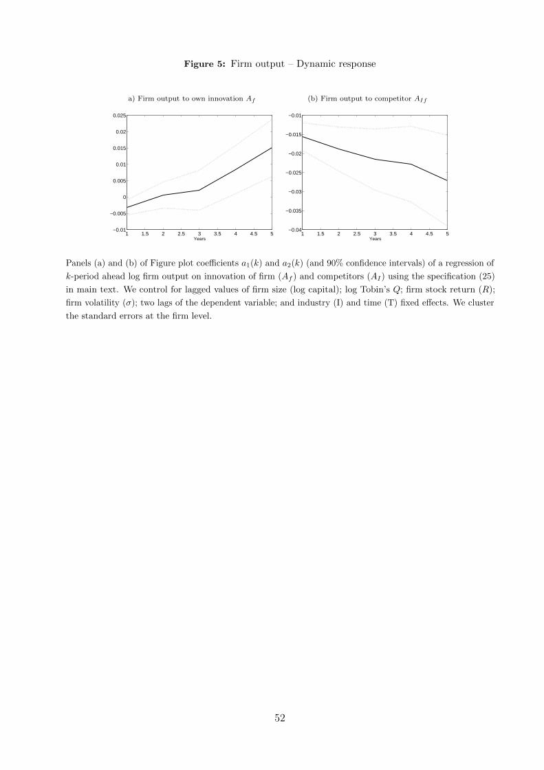
Figure 5: Firm output – Dynamic response

a) Firm output to own innovation Af (b) Firm output to competitor AIf

1 1.5 2 2.5 3 3.5 4 4.5 5−0.01

−0.005

0

0.005

0.01

0.015

0.02

0.025

Years1 1.5 2 2.5 3 3.5 4 4.5 5

−0.04

−0.035

−0.03

−0.025

−0.02

−0.015

−0.01

Years

Panels (a) and (b) of Figure plot coefficients a1(k) and a2(k) (and 90% confidence intervals) of a regression of

k-period ahead log firm output on innovation of firm (Af ) and competitors (AI) using the specification (25)

in main text. We control for lagged values of firm size (log capital); log Tobin’s Q; firm stock return (R);

firm volatility (σ); two lags of the dependent variable; and industry (I) and time (T) fixed effects. We cluster

the standard errors at the firm level.

52

Figure 6: Industry productivity – Dynamic response

(a) Capital productivity to own innovation AI (b) Capital productivity to aggregate AM

1 2 3 4 5 60

0.01

0.02

0.03

0.04

0.05

0.06

Years1 2 3 4 5 6

−0.09

−0.08

−0.07

−0.06

−0.05

−0.04

−0.03

−0.02

−0.01

0

0.01

Years

(c) Labor productivity to own innovation AI (d) Labor productivity to aggregate AM

1 1.5 2 2.5 3 3.5 4 4.5 5−0.01

0

0.01

0.02

0.03

0.04

0.05

0.06

Years1 1.5 2 2.5 3 3.5 4 4.5 5

−0.06

−0.05

−0.04

−0.03

−0.02

−0.01

0

0.01

0.02

Years

Figure plots coefficients a1(k) and a2(k) (and 90% confidence intervals) from a regression of k-period log

capital (panels a and b) and labor productivity (panels c and d) on amount of innovation AI at the industry

level, and the aggregate amount of innovation excluding that industry AM , using the specification (28) in

main text. We control for industry stock returns; the cross-sectional average of idiosyncratic volatility σ at

the industry level; and one lag of the dependent variable. Data is from Dale Jorgenson’s 35-sector KLEM.

We compute standard errors clustered by industry.

53

Figure 7: Industry output – Dynamic response

(a) Industry output to own innovation AI (b) Industry output to other industry innovation AIM

1 1.5 2 2.5 3 3.5 4 4.5 50

0.01

0.02

0.03

0.04

0.05

0.06

0.07

0.08

0.09

Years1 1.5 2 2.5 3 3.5 4 4.5 5

−0.1

−0.09

−0.08

−0.07

−0.06

−0.05

−0.04

−0.03

−0.02

−0.01

0

Years

Figure plots coefficients a1(k) and a2(k) (and 90% confidence intervals) of a regression of k-period ahead log

firm output on innovation of industry (AI) and innovation of other industries (AMI) using the specification

in equation 29. We control for industry stock return; the cross-sectional average of idiosyncratic volatility σ

at the industry level; and two lags of the dependent variable. Data is from Dale Jorgenson’s 35-sector KLEM.

Output is measured as value added in constant prices. We compute standard errors clustered by industry.

54

Figure 8: Innovation and Industry Growth

0 0.05 0.1 0.15 0.2 0.25

−0.04

−0.02

0

0.02

0.04

0.06

0.08

A, average (1960-1982)

∆lnY,average(1983-2005)

AgricMetalMine

Coal

Oil

MineConst

Food

Smoke

Txtile

Clothes

Wood

Furniture

PaperPrintChem

Refine

Rubber

Leather

Stone

MetalFabr

Mach

Elec. Mach

Auto

Trans. Equip.

InstrMisc Manuf

Trans

Comm

Elec Utilities

Gas Utilities

TradeFinance

Bus. Services

Figure plots the average output growth rate of 34 industries during the 1983-2006 period, versus the amount

of innovation in 1960-1982. We use our innovation measure adjusted for measurement error A. Data is from

Dale Jorgenson’s website. Output is measured as value added in constant prices.

55

Figure 9: Impulse responses, Productivity

0 1 2 3 4 5 6 7 80

0.002

0.004

0.006

0.008

0.01

0.012

0.014

0.016

0.018

Years0 1 2 3 4 5 6 7 8

0

0.005

0.01

0.015

0.02

0.025

0.03

Years

(a) VAR (b) VECM

Figure shows impulse response of productivity from a bi-variate VAR (left) or VECM (right) containing total

factor productivity and our aggregate innovation measure constructed using equation (31) in the main text.

We obtain impulse responses by ordering our innovation measure last. We include a deterministic trend in

the VECM. We select lag length based on the AIC criterion. Dotted lines represent 90% confidence intervals

using standard errors are computed using 500 bootstrap simulations.

56

Figure 10: Impulse responses, Output

0 1 2 3 4 5 6 7 8−0.02

−0.01

0

0.01

0.02

0.03

0.04

0.05

0.06

Years0 1 2 3 4 5 6 7 8

−0.01

0

0.01

0.02

0.03

0.04

0.05

0.06

0.07

0.08

0.09

Years

(a) VAR (b) VECM

Figure shows impulse response of aggregate output from a bi-variate VAR (left) or VECM (right) containing

output and our aggregate innovation measure constructed using equation (31) in the main text. We obtain

impulse responses by ordering our innovation measure last. We include a deterministic trend in the VECM.

We select lag length based on the AIC criterion. Dotted lines represent 90% confidence intervals using

standard errors are computed using 500 bootstrap simulations.

57

Figure 11: Impulse responses, Consumption

0 1 2 3 4 5 6 7 8−0.015

−0.01

−0.005

0

0.005

0.01

0.015

0.02

Years0 1 2 3 4 5 6 7 8

−0.01

−0.005

0

0.005

0.01

0.015

0.02

Years

(a) VAR (b) VECM

Figure shows impulse response of consumption from a bi-variate VAR (left) or VECM (right) containing

consumption and our aggregate innovation measure constructed using equation (31) in the main text. We

obtain impulse responses by ordering our innovation measure last. We include a deterministic trend in the

VECM. We select lag length based on the AIC criterion. Dotted lines represent 90% confidence intervals

using standard errors are computed using 500 bootstrap simulations.

58

Data Appendix

Patent Data

We download the entire history of U.S. patent documents from Google Patents. Using textanalysis algorithms, we match all patents in the Google data to corporations whose returnsare in the CRSP database. In addition, we extract the USPTO technology classes and numberof forward citations from the document. We merge our extracted citations data to dataprovided by Tom Nicholas. See the Online Appendix for more details.

Stock Market and Financial Data

The return data used to assess the stock market response to news about patents are fromCRSP over the period 1926–2010. In several of our analyses we use financial and accountingdata that are from Compustat. The sample in these cases is determined by the availability ofCompustat data (available from 1951 onwards). As is standard, we omit financial firms andutilities from our analysis.

Business-cycle data

Productivity is utilization-adjusted TFP from Basu et al. (2006). Populations is from theU.S. Census Bureau (http://www.census.gov/popest/national/national.html). Output andconsumption are from the Bureau of Economic Analysis. Output is gross domestic product(NIPA Table 1.1.5) divided by the consumption price index (St Louis Fed, CPIAUCNS).Consumption is consumption of non-durables plus services, deflated by the price index of non-durables and services respectively (NIPA Tables 1.1.5, 2.3.4). To get hours worked, we mergeseries CEU0500000007 and EEU00500005 from the BLS, times total private employment(BLS,CEU0500000001) divided by population. The aggregate Tobin’s Q is computed using NIPAand FRB Flow of Funds Data as in Laitner and Stolyarov (2003). Finally, the time seriesinformation on R&D expenditure spending in the US is obtained from the NSF website.

Industry Data

The industry-level data is from the KLEMS dataset of Dale Jorgenson. We use industryvalue added (constant prices) as measure of industry output.

Firm-level data

We define the investment rate as capital expenditures (Compustat: capx) divided by laggedgross property, plant and equipment (ppegt); labor hiring as the percentage change in thenumber of employees (emp); financial capital inflows as debt issuance plus equity issuanceminus payout (Compustat sstk + dltis - prstkc-dv-dltr) normalized by assets (at); return onassets as operating income (ib) plus depreciation divided by lagged gross property, plant andequipment; Tobin’s Q as the sum of the market value of common equity (CRSP Decembermarket capitalization), the book value of debt (dltt), the book value of preferred stock(pstkrv), minus the book value of inventories (invt) and deferred taxes (txdb), divided bygross property, plant and equipment (ppegt); productivity of capital as sales (sale) pluschange in inventories (invt) over gross property, plant and equipment (ppegt); productivityof labor as sales (sale) plus change in inventories (invt) over number of employees (emp).

59

Online Appendix to “Technological Innovation,

Resource Allocation and Growth”

Leonid Kogan, Dimitris Papanikolaou,

Amit Seru and Noah Stoffman

A Patent Data

Our measure of innovation relies on using information on patents that a firm creates and the stock

market response to news about these patents. We now discuss the data that we employ in our

analysis.

Patents in the United States are granted by the United States Patent and Trademark Office

(USPTO). We download the entire history of U.S. patent documents from Google Patents.1 Each of

about 7.8 million patent files was downloaded using an automation script.2

To construct our measure of innovation, we match all patents in the Google data to corporations

whose returns are in the CRSP database. Patent regulations require that only an individual, not a

corporation, can be an inventor. However, the inventor can assign the granted property rights to a

corporation or another person. Therefore, when patents are granted they always have an inventor,

and sometimes an “assignee”, that is, one or more corporations or persons.

For most patents, Google provides a text version of the patent document, created using OCR

software. We use this text version of the document to extract the names of corporations to

which patents are assigned. However, OCR technology is imperfect, and many of the downloaded

documents include a great deal of garbled text. We therefore make use of a number of text analysis

algorithms to extract relevant information from the documents.

Our sample covers patents granted between 1926 and 2010 matched to firms with returns in

CRSP database. Since we merge our patent data with data on stock returns, we are limited to the

period after 1926, when the CRSP database begins.

1http://www.google.com/patents

2Google also makes available for downloading bulk patent data files from the USPTO. The bulk data does not haveall of the additional “meta” information including classification codes and citation information that Google includes inthe individual patent files. Moreover, the quality of the text generated from Optical Character Recognition (OCR)procedures implemented by Google is better in the individual files than in the bulk files provided by the USPTO. Asexplained below, this is crucial for identifying patent assignees.

Matching patents to firms

Here, we briefly discuss the steps our matching procedure followed, and provide extensive details

Section C. We search the document for the words “assignee” or “assigned” and extract the text that

immediately follows. This text is either a company name, or the name of an individual to whom the

patent is assigned. We then count the number of times each assignee name appears across all patent

documents. We compare each assignee name to more common names, and if a given name is “close”,

in the sense of the Levenshtein distance, to a much more common name, we substitute the common

name for the uncommon name.3 For example, one of the most common names is “General Electric

Company”, which is associated with over 43,000 patents. We substitute this name for the far less

common, but quite similar, names “General Electbic Oohpany”, “General Electbic Cqhpany”, and

“Genebal Electbic Compakt”.

At this point, we have an assignee name for each patent. These names must be matched to

a company identifier such as the CRSP permco. This is accomplished in two steps. We begin by

looking only at patents that are also in the NBER database. For each assignee name identified

in the steps above, we count how many different permcos are matched to patents in the NBER

database. For example, all of the patents with an assignee name “General Electric Company” are

matched to one permco in the NBER database. We can therefore safely assume that all of the

patents assigned to the General Electric Company can be matched to that permco, even for patents

not included in the NBER data. Remaining assignee names are matched to CRSP firm names using

a name matching algorithm.4 The algorithm uses a score based on the inverse word frequency to

match assignee names to possible company names. For example, the word “American” is quite

common in company names, and so contributes little to name matching; the word “Bausch” is quite

uncommon, so it is given much more weight. Visual inspection of the matched names confirms very

few mistakes in the matching.

Extracting patent citations

We extract patent citations from three sources. First, all citations for patents granted between 1976

and 2011 are contained in text files available for bulk downloading from Google. These citations

are simple to extract and likely to be free of errors, as they are official USPTO data. Second, for

patents granted before 1976, we extract citations from the OCR text generated from the patent files.

We search the text of each patent for any 6- or 7-digit numbers, which could be patent numbers.

We then check if these potential patent numbers are followed closely by the corresponding grant

date for that patent; if the correct date appears, then we can be certain that we have identified

a patent citation. Since we require the date to appear near any potential patent number, it is

3The Levenshtein distance is the number of edits required to make one string match another string, where an editis inserting, deleting, or substituting one character.

4The algorithm is based on code written by Jim Bessen, available at http://goo.gl/m4AdZ.

2

unlikely that we would incorrectly record a patent citation – it is far more likely that we would fail

to record a citation than record one that isn’t there. Third, we complement our citation data with

the hand-collected reference data of Nicholas (2008). See Section C of this Appendix for a detailed

explanation of this process.

Summary statistics

We now provide some statistics that lend credence to our method for extracting patent information.

Table 1 shows the number of patents we match to companies. Of the 6.2 million patents granted in

or after 1926, we find the presence of an assignee in 4.4 million. The matching procedure provides

us with a database of 1.9 million matched patents, of which 523,301 (27%) are not included in the

NBER data. Figure 1 graphs the total number of patents matched by the year the patent was

granted. Patents included in the NBER data, which is the most comprehensive database previously

available, are shown in light shading. Patents unique to our database are presented in dark shading.

Note that the two sets of data appear to fit together fairly smoothly, and that even during the

period covered by the NBER data, our database adds an average of 2,187 patents to the NBER

data.5

Table 2 provides additional summary statistics. Overall, our data provides a matched permco

for 66% of all patents with an assignee, or 31% of all granted patents. By comparison, the NBER

patent project provides a match for 32% of all patents from 1976–2006, so our matching technique

works quite well, even using only data extracted from OCR documents for the period before the

NBER data. Another point of comparison is Nicholas (2008), who uses hand-collected patent data

covering 1910 to 1939. From 1926–1929, he matches 9,707 patents, while our database includes

8,858 patents; from 1930–1939 he has 32,778 patents while our database includes 47,036 matches

during this period.

B Other Data

Stock Market and Financial Data

The return data used to assess the stock market response to news about patents are from CRSP

over the period 1926–2010. In several of our analyses we use financial and accounting data that

are from Compustat. The sample in these cases is determined by the availability of Compustat

data (available from 1951 onwards). As is standard, we omit financial firms and utilities from our

analysis.

5We use information on the patent-assignee match in the NBER data to assist with our matching, so the matchduring the overlapping period is mostly the same, by construction. An exception is for cases where there is apparentlya mistake in the NBER match and our patent-assignee frequency-based matching system corrects an error.

3

Business-cycle data

Productivity is utilization-adjusted TFP from Basu, Fernald, and Kimball (2006). Populations is

from the U.S. Census Bureau (http://www.census.gov/popest/national/national.html). Output and

consumption are from the Bureau of Economic Analysis. Output is gross domestic product (NIPA

Table 1.1.5) divided by the consumption price index (St Louis Fed, CPIAUCNS). Consumption is

consumption of non-durables plus services, deflated by the price index of non-durables and services

respectively (NIPA Tables 1.1.5, 2.3.4). To get hours worked, we merge series CEU0500000007 and

EEU00500005 from the BLS, times total private employment(BLS, CEU0500000001) divided by

population. The aggregate Tobin’s Q is computed using NIPA and FRB Flow of Funds Data as in

Laitner and Stolyarov (2003). Finally, the time series information on R&D expenditure spending in

the US is obtained from the NSF website.

Industry Data

The industry-level data is from the KLEMS dataset of Dale Jorgenson. We use industry value added

(constant prices) as measure of industry output.

Firm-level data

We define the investment rate as capital expenditures (Compustat: capx) divided by lagged gross

property, plant and equipment (ppegt); labor hiring as the percentage change in the number of

employees (emp); financial capital inflows as debt issuance plus equity issuance minus payout

(Compustat sstk + dltis - prstkc-dv-dltr) normalized by assets (at); return on assets as operating

income (ib) plus depreciation divided by lagged gross property, plant and equipment; Tobin’s Q

as the sum of the market value of common equity (CRSP December market capitalization), the

book value of debt (dltt), the book value of preferred stock (pstkrv), minus the book value of

inventories (invt) and deferred taxes (txdb), divided by gross property, plant and equipment (ppegt);

productivity of capital as sales (sale) plus change in inventories (invt) over gross property, plant

and equipment (ppegt); productivity of labor as sales (sale) plus change in inventories (invt) over

number of employees (emp).

4

C Patent Data Construction – Details

In this section we explain in detail how we constructed our new patent data set. The raw data are

very large and not very well structured, and thus required a great deal of effort to clean. We used a

number of techniques to extract, clean, and match assignees from patents. As with any such project

there is a trade-off between type-I and type-II errors (in this case, failing to match an assignee to

CRSP or incorrectly matching an assignee to CRSP). Our approach was to be as conservative as

possible, attempting to minimize mismatches while at the same time extracting as many correct

matches as possible.

C.1 Data sources

We use three sources of data to construct the new patent database:

1. Details of patents granted from 1976–2010 is available in high-quality text files available for

bulk downloading from Google, through a special data-hosting arrangement with the United

States Patent and Trademark Office (USPTO). The text files use one of two data structures

that allows relatively straightforward data extraction: files for 2001–present use XML, while

files for 1976–2000 use a fixed-width data structure with labeled fields.

2. Patents granted prior to 1976 are also stored on Google, but only in individual web pages

(one per patent). Information during this period is drawn from Optical Character Recognition

(OCR) of original patent documents, and is of highly-variable quality. There is very limited, if

any, structure to these files.

3. We use the NBER patent data (Hall and Trajtenberg, 2001), which covers the period 1976–2006,

to help with the matching and to validate our other data extraction methods.

Due to varying data sources and quality over time, it worth stressing that from 1976–2010 we

use the official records of the USPTO. As we discuss below, we are able to provide some additions

and corrections to the NBER data during the period of overlap with our data. Prior to 1976 the

data are more difficult to work with, but we have implemented a number of sophisticated text

analysis algorithms to create a very high-quality database.

Downloading individual patent files

We downloaded individual patent data from Google. The URL for each patent’s summary page is of

the form http://www.google.com/patents/?id=RD0yAAAAEBAJ, where RD0y is a 4-character code

used by Google to identify each patent. The IDs use any of the characters {a, . . . , z, A, . . . , Z, 0,

. . . , 9, , -}. There are 644 = 16.8 million possible IDs, but only about 8 million patents. However,

5

all 16.8 million URLs must be checked, because there is no publicly-available mapping of patent

numbers to the Google ID.

A screen shot of the summary page for the patent with id RD0y, which is patent 4,345,262, is

shown in Figure 1. The main page includes—when available—the title of the patent, the filing and

grant dates, the abstract, inventor(s), original assignee(s), current classifications, and a record of

citations (out-cites) and references (in-cites). The information reported on this page by Google was

gleaned from the OCR analysis of the original patent document, and consequently less information

is reported for older documents, especially patents granted before 1976.

Figure 1: Google summary page for U.S. patent 4,345,262

Using a Perl automation script, we sequentially navigated to each of the 16.8 million patent

summary pages.6 From this page, we stored all available information. The script then loaded the

“Read this patent” link, which loads a PDF version of the patent document. From here, we loaded

the “plain text” version of the document, which is simply the text derived from OCR of the PDF

document. Examples of these pages are shown in Figures 2 and 3. We saved the complete text

of the plain text version of each patent. After compression, the complete archive of text requires

6Google generally blocks users from downloading so many web pages. We are grateful to Hal Varian for hisassistance with arranging permission to access these pages.

6

approximately 56 gigabytes of disk space.

Figure 2: PDF view

Figure 3: Plain text view

Download bulk patent files

As part of a special arrangement with the USPTO, Google also makes available for downloading bulk

patent data files. The bulk data does not have all of the additional “meta” information including

classification codes and citation information that Google includes in the individual patent files.

7

Moreover, the quality of the text generated from OCR procedures implemented by Google is better

in the individual files than in the bulk files provided by the USPTO. We therefore do not use the

bulk download files for data in the pre-NBER period.

For the post-NBER period, however, the bulk data files are of extremely high quality because

they are based on digital patent records as opposed to OCR data drawn from images of patent

documents. These data files are provided either in XML format or in a fixed-width record format.

In both cases, all fields (inventor name, grant date, etc.) are clearly identified. We rely on these

files to construct the database during the post-NBER period (2006–2009) and to make additions

and corrections to the NBER data.

C.2 Identifying assignees

Extracting assignee names

For data during the post-1976 period, we can use the XML files available for bulk download to

identify the assignee with virtually no errors.

During the pre-1976 period, we cannot rely solely on Google’s extraction of the filing and grant

dates or the assignee name because the OCR for patents frequently has errors. As an example,

consider patent 1,131,249, shown in Figure 4.

Figure 4: Title page of patent 1,131,249

It is clear to a human reader that this patent was assigned to the Allis-Chalmers Manufacturing

Company, but the OCR for this patent reads

EASLS B. KNIGHT, OF NORWOOD, OHIO, ASSIGNOR,, BY MESH’S ASSIGN1IBNTS, TO ALUSCHALME&S

MANOTAC/rURING- COMPANY, A COBPOBAT’lOH OF DELAY/ABE.

8

Consequently, Google records the assignee as “BY MESH S ASSIGNIIBNTS”, which is clearly not

accurate.

We therefore rely on a number of textual analysis algorithms to extract the assignee name from

the full text files we saved for each patent. In general, our approach to performing a “fuzzy” match

on a text string is to use the maximum likelihood n-gram approach described by Norvig (2009).

We begin by identifying the text where the assignee, if there is one, will be named. We do this

by searching for words that appear similar to “assign”, “assignor”, or “assignee”. When found near

the beginning of the patent document, this word is typically followed closely by the name of the

assignee, so we extract a text string of 200 characters for further processing. The assignee may be a

person, or a corporation, in which case the name will include a word like “company”, “corporation”

or “incorporated”. If the word “assign” and its variants are not found, we assume the inventor did

not assign the patent to another entity.

Cleaning assignee names

After extracting the string that is likely to contain the assignee name, additional cleaning is necessary.

Because of OCR errors, company names may be garbled. For example, the General Electric Company,

which has more than 43,000 patents in our data, appears as “General Electbic Oohpany”, “General

Electbic Cqhpany”, and “Genebal Electbic Compakt”, among hundreds of other misspellings. To

fix these, we first count how many patents have been granted to each assignee name, regardless of

how the assignee name is spelled. In this example, General Electric Company appears in 42,693

patents, while each of the misspelled variants appears fewer than 5 times.

We then calculate the Levenshtein edit distance7 between each assignee name and all other

names that have more patents. If any assignee name is close to another assignee name that is

associated with many more patents, then the more common assignee name is substituted for the

less common name. This algorithm correctly identifies all of the misspellings noted above as being

General Electric.

After cleaning assignee names, we manually checked which misspelled names were matched to

the 500 assignees with the most patents to confirm that no significant errors were introduced in this

step.

7The Levenshtein distance is the number of edits required to transform one string into another string, whereallowed edits are inserting, deleting, or substituting one character. For example, the Levenshtein distance between“patent” and “parent” is 1, while the distance between “patent” and “apparent” is 3.

9

Matching to CRSP

Having extract a list of assignee names, the next step is to match company names to the CRSP

permco identifier. This is accomplished in three steps.

We begin by looking only at those patents that are included in the NBER patent database.

For each assignee name identified in the steps above, we count how many different permcos are

matched to patents in the NBER database. For example, all of the patents with an assignee name

“General Electric Company” are matched to one permco in the NBER database. We can therefore

safely assume that all of the patents assigned to the General Electric Company can be matched to

that permco, even for patents not included in the NBER data. This step allows us to draw on the

extensive data cleaning and matching project undertaken by Hall and Trajtenberg (2001) while at

the same time identifying some errors in the NBER database. For example, patent 4,994,660 was

assigned to General Electric but is identified in the NBER data as being assigned to Hitachi, Ltd.

Because our algorithm relies on name matching, and the assignee name in that patent is General

Electric, the patent is correctly identified in our data.

The first step only helps us match assignees with patenting activity during the period covered by

the NBER database. We therefore proceed with a second step to match remaining assignee names.

We do this with a name matching algorithm based on code written by Jim Bessen, available at

http://goo.gl/m4AdZ. The algorithm uses a score based on the inverse word frequency to match

assignee names to possible company names. For example, the word “American” is quite common in

company names, and so contributes little to name matching; the word “Bausch” is quite uncommon,

so it is given much more weight. Visual inspection of the matched names confirms very few mistakes

in the matching.

Finally, we identify the top 250 assignees (by patents) with no CRSP matches. We manually

matched these to CRSP whenever possible. Examples of firms requiring manual matching include

research subsidiaries such as 3M Innovative Properties Company, which was not successfully matched

to CRSP because its name differs substantially from its parent. Although we only checked 250

assignees, this manual check allowed us to match an additional 64,000 patents. Firms with high

patenting activity but not matched to CRSP are either private companies or foreign firms that are

not listed on U.S. exchanges, an example of which is Hoffmann-La Roche, the large Swiss drug

company.

10

C.3 Correcting grant dates

The filing and grant dates of the patents are subject to the same sort of OCR errors as the assignee

information. The grant dates are particularly important for our purposes because we use them to

calculate the return around the grant date. Since patent numbers are sequential by grant dates, it

is easy to infer missing or incorrect grant dates by comparing patent dates to the grant dates of

adjacent patents. The same is not true of filing dates, but do not use filing dates in our current

work.

To populate missing patent dates and correct mistakes we identify the 3 non-missing grant dates

immediately preceding and following each patent. For example, if patent k’s grant date is missing

but patents (k − 3,. . . ,k − 1,k + 1,. . . ,k + 3) have grant date D, then we set patent k’s grant date

to D. By applying this procedure iteratively we are able to correct most grant dates, with the

exception of patents whose grant dates are missing and lie at a boundary between two grant dates.

We fill in these missing boundary dates by manually checking their grant dates on the USPTO’s

web site.

While we don’t rely on filing dates in the paper, it is possible to correct large errors in filing

dates by identifying cases where filing dates occur after the grant date, or much earlier than the

filing dates of adjacent patents. These errors often occur only in the year, so we can keep the

recorded month and day the same while setting the year of the patent filing to the median filing

year of a 20-patent window centered on a patent with an apparent error.

C.4 Extracting citations

Extracting patent citations from the patent text documents presents another challenge. The format

of a patent document has changed several times, as has the location and formatting of citations

within the document. For example, Figure 5 shows the references section of patent 2,423,030, granted

in 1947. The format seen here is the first format used after patent citation began in February, 1947.

A human reader has no problem identifying the citations in this patent. But to understand the

considerable challenge faced in automating this identification, consider the OCR for this part of the

patent:

other side. 35 REFERENCES CITED

By this invention I am able satisfactorily and The following references are of record in the

conveniently to effect the drying of’Shaped pot- jjle of tllis patent:

tery or other ceramic articles either in their

11

Figure 5: A patent citation section

moulds or otherwise, in a manner which min- UNITED STATES PATENTS

imises risk of injury by excessively rapid heating 40 Number Name Date

or moisture extraction. The invention is not, 1,767,872 Pox June 24, 1930

however, restricted to the example described as 1^934,904 Barnett et al Nov. 14’, 1933

subordinate details may be modified to suit dif- 2,257,180 Mayer Sept. 30, 1941

ferent requirements. 1,893,963 Russ Jan. 10,1933

Having thus described my invention what I 45

claim as new and desire to secure by Letters Pat- * ("uu-^ f A 1 Jun 11>

entis: Number Country Date

1. Means for drying ceramic ware, comprising 439,577 Great Britain Dec. 10,1935

Our approach is to identify any text that could be a patent number (a 6- or 7-digit number,

perhaps separated by commas, spaces, or other “noise” characters) and is closely followed by the

correct grant date for the cited patent. In particular, for every potential patent number we identify,

we determine its grant date and then search near the possible citation for that date. If the date

appears, we can be very confident that we have correctly identified a citation. For example, for the

patent shown in Figure 5 we extract the patent number 1,767,872 and then confirm that its grant

date—June 24, 1930—appears somewhere nearby in the text. By using this two-step process to

identify citations, our citation extraction is of very high quality—the probability that some random

7-digit number will be followed closely by the correct date is clearly extremely small.

Our citation extraction method provides more citations than what is available on the Google

summary page. For example, the Google summary page for the patent shown in the previous

example provides no citations at all, while our algorithm correctly extracted all four citations. (We

exclude citations to foreign patents, as these patents are not in our database.) In general, Google

does not currently report out-cites from patents granted before 1976, so we use this extraction

method on all patents granted between 1926 and 1975.

12

C.5 Data validation

As previously mentioned, any data extraction project such as this can lead to two types of errors:

matching a patent to a firm that is not the assignee, or failing to match a patent to a any firm when

it does have an assignee. Our strategy makes the first error very unlikely, as a match occurs only

when a name closely resembling a CRSP company name appears around the word “assignee” at the

beginning of patent document. We cannot be sure how many errors of the second type we made,

but we have taken care to ensure that our algorithms allow as flexible matching as possible.

We also did two final checks to check the quality of our matching strategy. First, we visually

inspected a random sample of 500 patents granted between 1926 and 1975 and confirmed that

assignees had been correctly extracted, and correctly matched if the assignee appeared in CRSP.

This is obviously a very small sample of patents, but this careful check confirmed that no serious

errors existed.

Second, we applied the extraction and matching algorithms we used in the pre-1976 period to a

random sample of 25,000 patents granted between 1976 and 1999. We then compared our matches

to the matches in the NBER data. None of our matches was incorrect, and only 3 patents were

incorrectly not matched to an assignee. In other words, applying the techniques we used on pre-1976

data to data from the NBER period yields results that are virtually identical to those in the NBER

database.

13

D Analytical Appendix

Here, we provide the derivation of the theoretical results in Section 2.1. The final-good producer

solves the intra-period profit maximization problem

maxLFt ,{qjt}

Zt(LFt)1−α ∫ Ht

0(θj)

1−α (qjt)α dj −

∫ Ht

0pjtqjtdj − wtLFt .

The associated optimality conditions for intermediate good inputs dictate that the price of interme-

diate goods pj is equal to

Zt(LFt)1−α

(θj)1−α α (qjt)

α−1 = pjt

and therefore

qjt = LFt θj

(pjtαZt

) 1α−1

.

If a good is covered by a patent, the monopolist producer maximizes intra-period profits, taking

production plans for all other goods as given:

maxpjt

(pjt − wt)LFt θj(pjtαZt

) 1α−1

,

which implies the equilibrium spot price

pjt =wtα.

and hence the equilibrium output of an intermediate good covered by a patent is

qjt = LFt θj

(wtα2Zt

) 1α−1

.

The equilibrium output of an intermediate good not covered by a patent is

qjt = LFt θj

(wtαZt

) 1α−1

.

The optimality condition with respect to the labor input in the final-good firm’s problem is

(1− α)Yt = wtLFt .

14

Substituting into this relation the equilibrium output of intermediate goods, we find

wtLFt = (1− α)

(LFt)1−α

Zt

∫ Ht

0 pjθj

(LFt

(wtα2Zt

) 1α−1

)αdj+∫ Ht

0 (1− pj) θj(LFt

(wtαZt

) 1α−1

)αdj

= (1− α)LFt Zt

HtE [pjθj ]

((wtα2Zt

) 1α−1

)α+

Ht (1− E [pjθj ])

((wtαZt

) 1α−1

)α

and therefore the equilibrium wage is given by

wt = (1− α)1−α Zt

{∫ Ht

0pjθjα

2α1−αdj +

∫ Ht

0(1− pjθj)α

α1−αdj

}1−α

= B0Zt (Ht)1−α ,

where

B0 = (1− α)1−α{

E [pjθj ]α−2αα−1 + (1− E [pjθj ])α

−αα−1

}1−α.

The market clearing condition in the labor market that determines the equilibrium allocation of

labor between production of the final good and production of the intermediate goods is

LFt +

∫ Ht

0qjtdj = 1,

hence

LFt

{1 +

(E [pjθj ]α

21−αB

1α−1

0 + (1− E [pjθj ])α1

1−αB1

α−1

0

)}= 1

and

LFt = B1 ≡{

1 +

(E [pjθj ]α

21−αB

1α−1

0 + (1− E [pjθj ])α1

1−αB1

α−1

0

)}−1

In summary, the equilibrium output of an intermediate good covered by a patent is

qjt = B1

(B0α

−2) 1α−1

(θjH

−1t

).

and the equilibrium output of an intermediate good not covered by a patent is

qjt = B1

(B0α

−1) 1α−1

(θjH

−1t

).

15

The equilibrium output of the final consumption good is

Yt = (1− α)−1wtB1 = (1− α)−1B0B1Zt (Ht)1−α = B2Zt (Ht)

1−α ,

where

B2 = (1− α)−1B0B1.

Next, we determine the stock market reaction to a successful patent application. A monopolistic

producer of an intermediate good j generates equilibrium profits equal to

Hτ(j) −Hτ(j)−1

δ(pjt − wt) qjt =

Hτ(j) −Hτ(j)−1

δwt(α−1 − 1

)qjt

=Hτ(j) −Hτ(j)−1

δB0Zt (Ht)

1−α (α−1 − 1)B1

(B0α

−2) 1α−1

(θj (Ht)

−1)

=Hτ(j) −Hτ(j)−1

δB3θjZt (Ht)

−α ,

where

B3 = Bαα−1

0 B1

(α−1 − 1

)α

21−α .

The equilibrium stochastic discount factor, based on the household’s optimality conditions, is

Mt = ρ−t (Yt)−γ = ρ−t

(B2Zt (Ht)

1−α)−γ

.

Therefore, the time-t present value of profits generated by the patent-protected good j (including

the current period) is

B3

Hτ(j) −Hτ(j)−1

δθjEt

[ ∞∑s=0

Zt+s (Ht+s)−α ρ−s

(Zt+sZt

)−γ (Ht+s

Ht

)−γ(1−α)]

= B3

Hτ(j) −Hτ(j)−1

δθjZt (Ht)

−α Et

[1 +

∞∑s=1

ρ−s(Ht+s

Ht

)−γ(1−α)−α(Zt+sZt

)1−γ]

= (B3 +B4)Hτ(j) −Hτ(j)−1

δθjZt (Ht)

−α ,

where

B4 = B3Et

[ ∞∑s=1

ρ−se−(γ(1−α)+α)(∑sn=1 ∆ lnHn)−(γ−1)(

∑sn=1 ∆ lnZn)

].

16

We conclude that the cumulative stock market gain in response to successful patent applications in

period t – the sum of the individual stock firm responses ∆Vft,

∆Vft = (1− pj) (B3 +B4) χ−1 (Ht −Ht−1) θj ZtH−αt ,

is

∆Vt =

∫ Ht

Ht−1

(1− pj) (B3 +B4) θjZt (Ht)−α dj = (B3 +B4) (1− E [pjθj ])Zt (Ht)

−α (Ht −Ht−1)

= B5 (1− E [pjθj ])Zt (Ht)1−α

(1− e−∆ lnHt

),

where B5 = (B3 +B4) .

We normalize the aggregate market reaction by the total (ex-dividend) stock market value at the

end of period t to eliminate the effect of the aggregate disembodied productivity process Zt on the

stock market reaction to patent grants. The time-t stock market value is

Pt = Et

∞∑s=1

∫ Ht+s

0

(B3θjZt+s (Ht+s)

−α)︸ ︷︷ ︸Cash flow

[ρ−s

(Zt+sZt

)−γ (Ht+s

Ht

)−γ(1−α)]

︸ ︷︷ ︸Discount factor

dj

= B3Zt (Ht)

1−α Et

[ ∞∑s=1

ρ−s(Ht+s

Ht

)(1−γ)(1−α)(Zt+sZt

)1−γ]

= B6Zt (Ht)1−α ,

where

B6 = B3Et

[ ∞∑s=1

ρ−se(1−γ)(1−α)(∑sn=1 ∆ lnHn)−(γ−1)(

∑sn=1 ∆Zn)

]

Therefore, the normalized aggregate stock market reaction to patent grants is

∆VtPt

=B5 (1− E [pjθj ])Zt (Ht−1)1−α e−α∆ lnHt

(e∆ lnHt − 1

)B6Zt (Ht)

1−α

= B7 (1− E [pjθj ])(

1− e−∆ lnHt),

where B7 = B5/B6.

For small values of ∆ lnHt, the term(1− e−∆ lnHt

)is approximately equal to ∆ lnHt.

17

The log growth of aggregate output during the same period is

lnYt − lnYt−1 = (1− α) ∆ lnHt + ∆ lnZt.

18

E Additional results and descriptive statistics

Table 1: Number of patents

Data step Number of patents

Total downloaded patents 7,797,506

Granted in 1926 or later 6,272,428

Identified as having an assignee 4,374,524

Matched to CRSP 1,928,123

Of which:

Present in NBER data 1,404,822

New to this paper 523,301

The table provides details on patents in our sample. We begin with all patents downloaded from Google Patents, and

restrict the sample to post-1926. Not all patents have assignees, and among those that do, not all are companies in

CRSP. We are able to match 1,928,123 patents to CRSP firms, of which 523,301 (27%) are new to this study. Further

details are reported in Table 2 and Figure 1.

19

Table 2: Assignee matching by Decade

Number of patents Number of unique

Years Total With assignee Matched to CRSP Matched firms CRSP firms

1926–1929 174,022 48,433 8,858 182 786

1930–1939 442,700 172,925 47,029 355 951

1940–1949 307,499 141,345 60,616 451 1,042

1950–1959 425,953 171,157 82,255 587 1,246

1960–1969 567,599 265,524 165,409 1,175 3,177

1970–1979 690,459 393,661 247,102 2,086 7,204

1980–1989 708,735 579,518 235,525 2,756 11,715

1990–1999 1,109,398 933,705 352,005 3,664 14,882

2000–2010 1,846,063 1,668,256 729,324 4,415 11,900

All years 6,272,428 4,374,524 1,928,123 7,864 26,660

The shows summary statistics for patents in our sample by decade. Column 2 shows the total number of patents, and

column 3 shows how many patents are identified as having an assignee. Column 4 shows how many of those patents

with assignees are matched to a company in CRSP. (The remaining assignees are either individuals, private companies,

or the matching process was unable to identify the correct company.) Columns 5 and 6 show how many unique firms

there are matched to patents or in CRSP.

20

Table 3: Stock turnover around patent announcement days

Event k = −1 k = 0 k = 1 k = 2 k = 3 k = 4

vol/shrout I. Turnover

A. Patent grant -0.147 -0.008 0.0502 0.0588 0.0487 -0.074

(-5.27) (-0.68) (3.63) (3.22) (1.78) (-4.65)

B. Patent publication 0.152 0.255 -0.194 -0.385 0.114 -0.205

(4.02) (5.51) (-3.03) (-4.17) (3.08) (-3.07)

vol/shrout− vol/shrout II. Relative turnover

A. Patent grant -0.156 -0.006 0.055 0.061 0.047 -0.091

(-6.74) (-0.57) (5.19) (4.24) (3.76) (-6.71)

B. Patent publication 0.130 0.182 -0.015 -0.335 0.085 -0.191

(4.33) (7.25) (-0.37) (-8.41) (2.73) (-5.75)

log(a+ vol/shrout) III. Log turnover

A. Patent grant -0.035 -0.004 0.013 0.016 0.021 -0.017

(-12.44) (-1.76) (6.45) (6.57) (7.35) (-7.00)

B. Patent publication 0.001 0.018 -0.019 -0.012 -0.009 -0.002

(0.13) (3.82) (-2.29) (-1.20) (-1.76) (-0.36)

log(a+vol/shrout

a+vol/shrout

)IV. Log relative turnover

A. Patent grant -0.037 -0.005 0.013 0.016 0.020 -0.023

(-16.14) (-2.59) (8.23) (8.12) (8.23) (-12.34)

B. Patent publication 0.016 0.024 0.011 -0.043 0.002 -0.025

(5.94) (9.49) (2.59) (-10.58) (0.49) (-7.45)

Table shows the output of the regression of variants of share turnover (xt+k = volt/shroutt) on a dummy variable

taking the value 1 if a patent was granted to the firm on day t (Panel A), or the USPTO publicized the grant

application of the firm on day t (Panel B). Each column in these panels represents a regression. We include firm-year

and day-of-week fixed effects. We cluster standard errors by year and report t-statistics in parenthesis. We restrict the

sample to firms that have been granted at least one patent.

21

Table 4: Which firms innovate?

Aft (1) (2) (3) (4)

lnKt−1 0.062 0.067 0.076 0.035

(39.55) (40.40) (43.12) (34.17)

lnQt−1 0.035 0.028 0.020

(19.82) (14.96) (20.11)

lnRDt−1 0.068 0.030

(28.38) (23.07)

Af,t−1 0.742

(88.33)

Observations 141695 141695 65234 65058

pseudo R2 0.644 0.671 0.739 1.242

Table shows Tobit regressions of firm-level innovation Aft on firm characteristics: log firm size (Kft, gross PPE), log

Tobin’s Q and log R&D expenditures to book assets lnRD. All specifications include year (T) and industry (I) fixed

effects. Standard errors are clustered by firm.

22

Table 5: Number of future citations and announcement day return: 5-day window

Five-day window – ([t, t+4])

Grant Day Publication Day

(1) (2) (3) (4) (5) (6) (7) (8)

log(1 +N) I. Log number of citations plus one

log A 0.037 0.195 0.106 0.054 0.030 0.048 0.036 0.013

(8.99) (5.79) (5.72) (5.21) (5.77) (5.79) (4.40) (1.17)

R2 0.289 0.295 0.401 0.426 0.244 0.249 0.317 0.355

A 1.543 0.412 0.102 0.361 0.224 -0.642 -0.323 -0.196

(8.49) (2.12) (1.85) (4.42) (1.74) (-3.99) (-1.81) (-1.14)

R2 0.285 0.293 0.400 0.426 0.239 0.248 0.318 0.355

(1) (2) (3) (4) (5) (6) (7) (8)

N II. Number of citations

log A 0.676 3.212 1.802 1.088 0.249 0.385 0.282 0.217

(7.75) (4.54) (4.72) (4.13) (3.96) (4.38) (4.28) (2.17)

R2 0.097 0.104 0.221 0.262 0.322 0.104 0.108 0.186

A 32.377 17.706 8.328 12.581 4.195 -1.764 -1.553 1.003

(6.36) (3.68) (2.66) (3.83) (2.04) (-1.53) (-1.73) (0.82)

R2 0.095 0.103 0.221 0.262 0.099 0.107 0.186 0.233

Controls

Fixed Effects T T TxC TxC,F T T TxC TxC,F

Volatility - Y Y Y - Y Y Y

Firm Size - Y Y Y - Y Y Y

# patents - Y Y Y - Y Y Y

granted same day

Table is the counterpart to Table 3 in the text, but we now use the five day (t, t+ 4) stock market reaction around the

patent grant day (columns 1-4) or the day the application is publicized by the USPTO (columns 5-8).

23

Table 6: Firm-level reallocation: raw stock market reaction

it+1 I. Investment

(1) (2) (3) (4) (5)

AIt 0.500 0.441 0.738 -0.982 -0.990

(2.75) (2.43) (4.29) (-4.53) (-4.56)

Aft 1.073 0.831 0.930 -0.302 -0.323

(7.12) (5.49) (6.37) (-2.08) (-2.23)

R2 0.084 0.091 0.220 0.259 0.260

nt+1 II. Labor hiring

(1) (2) (3) (4) (5)

AIt 2.274 2.210 2.317 0.251 0.226

(7.18) (7.02) (7.32) (0.73) (0.66)

Aft 2.637 2.375 2.198 0.556 0.510

(10.31) (9.32) (8.72) (2.21) (2.03)

R2 0.039 0.044 0.053 0.086 0.088

et+1 III. Financial inflows

(1) (2) (3) (4) (5)

AIt 1.809 1.853 2.017 1.160 1.122

(6.71) (6.88) (7.36) (4.30) (3.97)

Aft -0.020 0.159 0.150 -0.937 -0.808

(-0.07) (0.58) (0.55) (-3.41) (-2.96)

R2 0.114 0.117 0.155 0.184 0.219

Observations 126727 126727 126727 126727 126727

Fixed Effects I,T I,T I,T I,T I,T

(Size) Y Y Y Y Y

(σ) - Y Y Y Y

(xt) - - Y Y Y

(Rf , RI , Q) - - - Y Y

(ROA) - - - - Y

Table is the counterpart to firm level reallocation tables in main text, but we now construct our innovation measure

using the raw stock market reaction A instead of A.

24

Table 7: Firm-level reallocation: number of patents

it+1 I. Investment

(1) (2) (3) (4) (5)

PIt -0.365 -0.399 -0.266 -0.280 -0.281

(-5.63) (-6.05) (-5.68) (-5.99) (-6.02)

Pft 0.243 0.239 0.231 0.197 0.204

(9.63) (9.19) (12.03) (9.81) (10.12)

R2 0.085 0.092 0.220 0.260 0.261

nt+1 II. Labor hiring

(1) (2) (3) (4) (5)

PIt -0.118 -0.163 -0.157 -0.167 -0.166

(-1.42) (-1.96) (-1.98) (-2.13) (-2.14)

Pft 0.166 0.152 0.196 0.142 0.156

(5.52) (5.10) (6.94) (4.65) (5.12)

R2 0.038 0.044 0.053 0.086 0.088

et+1 III. Financial inflows

(1) (2) (3) (4) (5)

PIt -0.432 -0.407 -0.336 -0.380 -0.376

(-5.11) (-4.87) (-4.85) (-5.39) (-6.11)

Pft 0.182 0.184 0.174 0.118 0.054

(5.04) (5.23) (6.12) (3.60) (1.82)

R2 0.114 0.117 0.155 0.182 0.219

Observations 126727 126727 126727 126727 126727

Fixed Effects I,T I,T I,T I,T I,T

(Size) Y Y Y Y Y

(σ) - Y Y Y Y

(xt) - - Y Y Y

(Rf , RI , Q) - - - Y Y

(ROA) - - - - Y

Table is the counterpart to firm level reallocation tables in main text, but we now construct our innovation measure

using the total number of patents P granted to firm f in year t.

25

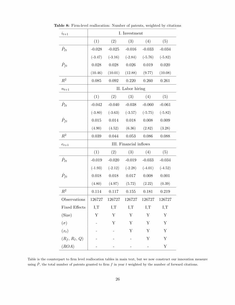
Table 8: Firm-level reallocation: Number of patents, weighted by citations

it+1 I. Investment

(1) (2) (3) (4) (5)

PIt -0.028 -0.025 -0.016 -0.033 -0.034

(-3.47) (-3.16) (-2.84) (-5.76) (-5.82)

Pft 0.028 0.028 0.026 0.019 0.020

(10.46) (10.01) (12.88) (9.77) (10.08)

R2 0.085 0.092 0.220 0.260 0.261

nt+1 II. Labor hiring

(1) (2) (3) (4) (5)

PIt -0.042 -0.040 -0.038 -0.060 -0.061

(-3.80) (-3.63) (-3.57) (-5.75) (-5.82)

Pft 0.015 0.014 0.018 0.008 0.009

(4.90) (4.52) (6.36) (2.82) (3.28)

R2 0.039 0.044 0.053 0.086 0.088

et+1 III. Financial inflows

(1) (2) (3) (4) (5)

PIt -0.019 -0.020 -0.019 -0.033 -0.034

(-1.93) (-2.12) (-2.28) (-4.01) (-4.52)

Pft 0.018 0.018 0.017 0.008 0.001

(4.80) (4.97) (5.72) (2.22) (0.39)

R2 0.114 0.117 0.155 0.181 0.219

Observations 126727 126727 126727 126727 126727

Fixed Effects I,T I,T I,T I,T I,T

(Size) Y Y Y Y Y

(σ) - Y Y Y Y

(xt) - - Y Y Y

(Rf , RI , Q) - - - Y Y

(ROA) - - - - Y

Table is the counterpart to firm level reallocation tables in main text, but we now construct our innovation measure

using P , the total number of patents granted to firm f in year t weighted by the number of forward citations.

26

Table 9: Firm-level productivity

zkt+1, zlt+1

I. Raw Measure

Capital Labor

(1) (2) (3) (4) (5) (6)

AIt 5.923 5.801 2.368 5.860 5.744 3.293

(10.49) (10.36) (3.90) (11.33) (11.17) (6.00)

Aft 3.671 3.205 1.555 2.088 1.700 0.691

(5.76) (5.03) (2.46) (3.55) (2.89) (1.18)

R2 0.844 0.845 0.847 0.847 0.848 0.849

zkt+1, zlt+1

II. Number of patents

Capital Labor

(1) (2) (3) (4) (5) (6)

PIt 0.064 -0.002 0.002 -0.179 -0.239 -0.241

(0.48) (-0.02) (0.02) (-1.53) (-2.04) (-2.04)

Pft 0.629 0.626 0.640 0.726 0.713 0.716

(11.90) (11.45) (11.63) (14.35) (13.76) (13.64)

R2 0.844 0.845 0.847 0.847 0.848 0.850

zkt+1, zlt+1

III. Number of patents, weighted by citations

Capital Labor

(1) (2) (3) (4) (5) (6)

PIt -0.026 -0.020 -0.041 -0.010 -0.004 -0.021

(-1.72) (-1.30) (-2.67) (-0.70) (-0.32) (-1.56)

Pft 0.062 0.062 0.061 0.076 0.075 0.074

(13.17) (12.87) (12.73) (16.49) (16.04) (15.64)

R2 0.844 0.845 0.847 0.848 0.849 0.850

Observations 125678 125678 125678 120020 120020 120020

Fixed Effects I,T I,T I,T I,T I,T I,T

(Size, xt−1) Y Y Y Y Y Y

(σ) - Y Y - Y Y

(Rf , RI , q) - - Y - - Y

Table is the counterpart to productivity regressions in the main text, but we now construct our innovation measure

using a) A, raw stock market reaction; b) P , the total number of patents granted to firm f in year t; c) P , the total

number of patents granted to firm f in year t, weighted by the number of forward citations .27

Table 10: Innovation and aggregate variables, OLS specifications

I. TFP growth

∆xt+T T=1 T=2 T=3 T=4 T=5 T=6

∆ lnAt 0.0027 0.0054 -0.0004 0.0014 0.0004 -0.0015

(2.42) (2.62) (-0.20) (0.56) (0.17) (-0.68)

R2 0.021 0.089 0.000 0.007 0.001 0.007

∆ lnAt 0.0031 0.0045 0.0006 0.0041 0.0010 -0.0005

(2.92) (2.68) (0.34) (4.05) (0.42) (-0.22)

∆xt 0.2334 0.0144 0.1485 0.1964 0.0400 0.0643

(3.33) (0.17) (1.73) (3.04) (0.40) (1.13)

R2 0.074 0.067 0.024 0.079 0.004 0.007

II. Output growth

∆yt+T T=1 T=2 T=3 T=4 T=5 T=6

∆ lnAt -0.0106 -0.0060 -0.0035 0.0066 0.0093 0.0059

(-1.93) (-0.67) (-0.54) (1.81) (2.26) (1.23)

R2 0.038 0.012 0.004 0.016 0.038 0.016

∆ lnAt -0.0058 -0.0027 0.0021 0.0076 0.0042 0.0056

(-1.19) (-0.29) (0.57) (2.02) (1.87) (1.02)

∆yt 0.4550 0.0631 -0.1702 -0.2828 -0.1515 0.0062

(5.34) (0.51) (-2.88) (-3.07) (-2.24) (0.07)

R2 0.234 0.007 0.040 0.139 0.044 0.014

III. Consumption growth

∆ct+T T=1 T=2 T=3 T=4 T=5 T=6

∆ lnAt -0.0081 -0.0043 -0.0024 0.0008 0.0034 0.0031

(-2.75) (-0.98) (-0.74) (0.41) (2.03) (1.96)

R2 0.131 0.037 0.013 0.002 0.040 0.038

∆ lnAt -0.0060 -0.0031 0.0011 0.0021 0.0021 0.0032

(-2.43) (-0.76) (0.77) (1.43) (1.42) (1.55)

∆ct 0.4687 0.1733 -0.0829 -0.2460 -0.0221 -0.0270

(5.82) (1.82) (-1.47) (-2.77) (-0.37) (-0.58)

R2 0.327 0.057 0.015 0.131 0.017 0.039

Table shows regressions of 1-period growth rate in z, T periods from now, ∆zt+T ≡ zt+T − zt+T−1 on log changes

in our innovation aggregate measure A. We show results for log TFP, output and consumption, z ∈ {x, y, c}. We

standardize changes in lnA to unit standard deviation. Standard errors are Newey-West, with automatic lag length

selection. 28

Figure 1: Number of Patents with Matched Assignees

Figure shows the number of patents matched to CRSP firms by year of patent grant. Light shading denotes patents

included in the NBER patent data set, while dark shading denotes patents that are new in our paper.

29

Figure 2: Firm innovation measures – Tail distribution

−2 −1 0 1 2 3 4−12

−11

−10

−9

−8

−7

−6

−5

−4

−3

−2

log A

log(1−

F(A

))

Figure plots the log complementary empirical cdf, log(1 − F (A)), versus the log value of the firm-level innovation

measure, logA, for the top 10 percent of the distribution.

30

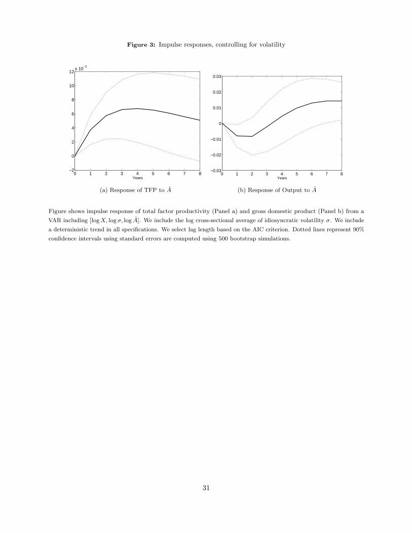
Figure 3: Impulse responses, controlling for volatility

0 1 2 3 4 5 6 7 8−2

0

2

4

6

8

10

12x 10

−3

Years0 1 2 3 4 5 6 7 8

−0.03

−0.02

−0.01

0

0.01

0.02

0.03

Years

(a) Response of TFP to A (b) Response of Output to A

Figure shows impulse response of total factor productivity (Panel a) and gross domestic product (Panel b) from a

VAR including [logX, log σ, log A]. We include the log cross-sectional average of idiosyncratic volatility σ. We include

a deterministic trend in all specifications. We select lag length based on the AIC criterion. Dotted lines represent 90%

confidence intervals using standard errors are computed using 500 bootstrap simulations.

31

Figure 4: Impulse responses, controlling for level of stock prices

0 1 2 3 4 5 6 7 8−4

−2

0

2

4

6

8

10

12

14

16x 10

−3

Years0 1 2 3 4 5 6 7 8

0

1

2

3

4

5

6

7

8x 10

−3

Years

(a) Response of TFP to M (b) Response of TFP to A

0 1 2 3 4 5 6 7 8−0.02

−0.01

0

0.01

0.02

0.03

0.04

0.05

Years0 1 2 3 4 5 6 7 8

0

0.005

0.01

0.015

0.02

0.025

0.03

0.035

0.04

0.045

Years

(c) Response of Output to M (d) Response of Output to A

Figure shows impulse response of total factor productivity (Panels a-b) and gross domestic product (Panels c-d) from

a VAR including [logX, logM, log A], where M is the stock market level deflated by the price deflator and population

growth, following Beaudry and Portier (2006). Right panel shows impulse response to our innovation measures. Left

panel shows response to per-capita real stock market level. We include a deterministic trend in all specifications. We

select lag length based on the AIC criterion. Dotted lines represent 90% confidence intervals using standard errors are

computed using 500 bootstrap simulations.

32

Figure 5: Impulse responses using Number of Patents and R&D Stock

0 1 2 3 4 5 6 7 80

1

2

3

4

5

6

7

8

9x 10

−3

Years0 1 2 3 4 5 6 7 8

−4

−2

0

2

4

6

8x 10

−3

Years

(a) No. patents - Productivity (b) R&D Stock - Productivity

0 1 2 3 4 5 6 7 8−0.02

−0.015

−0.01

−0.005

0

0.005

0.01

0.015

0.02

Years0 1 2 3 4 5 6 7 8

−8

−6

−4

−2

0

2

4

6x 10

−3

Years

(c) No. patents - Output (d) R&D Stock - Output

Left panel shows impulse response of log productivity and output from a bi-variate VAR [logXt, logNt] with a

deterministic trend. Right panel shows impulse response of log productivity and output from a bi-variate VAR

[logXt, logRDt] with a deterministic trend. Dotted lines represent 90% confidence intervals.

33

References

Basu, S., J. G. Fernald, and M. S. Kimball (2006). Are technology improvements contractionary?

American Economic Review 96 (5), 1418–1448.

Beaudry, P. and F. Portier (2006). Stock prices, news, and economic fluctuations. American

Economic Review 96 (4), 1293–1307.

Hall, B., A. J. and M. Trajtenberg (2001). The NBER patent citation data file: Lessons, insights

and methodological tools. Technical report, NBER Working Paper 8498.

Laitner, J. and D. Stolyarov (2003). Technological change and the stock market. The American

Economic Review 93 (4), pp. 1240–1267.

Nicholas, T. (2008). Does innovation cause stock market runups? Evidence from the great crash.

American Economic Review 98 (4), 1370–96.

Norvig, P. (2009). Natural langugage corpus data. In T. Segaran and J. Hammerbacher (Eds.),

Beautiful Data. O’Reilly Media.

34