technological change and depletion in offshore oil...
TRANSCRIPT
DRAFT
Technological Change and Depletion in Offshore Oil and Gas
Shunsuke Managi1, James J. Opaluch1, Di Jin2 and Thomas A. Grigalunas1
1Department of Environmental and Natural Resource EconomicsUniversity of Rhode Island
Kingston, Rhode Island 02881
2Marine Policy CenterWoods Hole Oceanographic Institution
Woods Hole, Massachusetts 02543
This research was funded by the United States Environmental Protection Agency STAR grantprogram (Grant Number Grant Number R826610-01) and the Rhode Island AgriculturalExperiment Station (AES # XXXX), and is Woods Hole Contribution Number 10583. Theresults and conclusions of this paper do not necessary represent the views of the fundingagencies.
December 2001
DRAFT
Technological Change and Depletion in Offshore Oil and Gas
Abstract
A critical concern for continued growth of the world economy is whether technological
progress can mitigate resource depletion. This paper measures depletion effects and
technological change for offshore oil production in the Gulf of Mexico using a unique field-level
data set from 1947-1998. The study supports the hypothesis that technological progress has
mitigated depletion effects over the study period, but the pattern differs from the conventional
wisdom for non-renewable resource industries. Contrary to the usual assumptions of monotonic
changes in productivity or an inverted “U” shaped pattern, we found that productivity declined
for the first 30 years of our study period. But more recently, the rapid pace of technological
change has outpaced depletion and productivity has increased rapidly, particularly in most
recent 5 years of our study period. We also provide a more thorough understanding of different
components of technological change and depletion.
JEL codes: D24, Q32, L71
Key words: technological change, depletion and offshore oil and gas industry
DRAFT
-2-
Technological Change and Depletion in Offshore Oil and Gas
Resource depletion is of critical importance for maintenance of the world economy.
Early studies from Malthus (1826) to the so-called Club of Rome report (Meadows et al, 1972),
have argued that limited resources will of necessity constrain economic growth. Typically, the
conclusions of these studies have been pessimistic with respect to the potential for continued
growth, even in the near term, and have called for a reorientation of policy towards development
of a “spaceship” economy (Boulding, 1966; Daly, 1991). Other more recent studies have
concluded that world production of critical resources such as petroleum will peak in the near
future, followed by an inevitable decline (e.g., Deffeyes, 2001).
However, these studies have been sharply criticized for understating the potential for
technological change to offset resource depletion (e.g., Cole, et al, 1975). These critiques have
argued that, at least in principal, an exponential growth in knowledge could provide a basis for
continued technological innovation that offsets resource depletion, and thereby fuel continued
growth for an indefinite period (e.g., Stiglitz, 1974; Barbier, 1999). Proponents of this latter
perspective have argued that the potential for technological progress to ameliorate resource
scarcity is an empirical issue. Related empirical studies using prices as indicators of resource
scarcity have found mixed results, with some studies supporting diminishing resource scarcity
(e.g., Barnet and Morse, 1963), while others have found the evidence to be mixed or
inconclusive (Slade, 1982; Berck and Roberts, 1996).
Empirical evidence regarding resource scarcity needs to consider more than physical
resource availability, but must also consider the net effects of resource depletion and
DRAFT
-3-
technological change. Hence, thorough conceptual and empirical analyses of technological
change are essential for identifying appropriate policy actions to be undertaken to mitigate
potential negative effects of resource depletion.
This paper uses field level data to measure technological change in offshore oil and gas
production in the Gulf of Mexico, and to test the hypothesis that technological change has
succeeded in offsetting depletion effects in offshore Gulf of Mexico petroleum production over
the past 50 years. This is an important area of application because energy supplies are critically
important resources supporting our economy, and because petroleum and natural gas are among
the most vital energy resources in today’s economy. We apply Data Envelopment Analysis
(DEA) to field level data in order measure changes in productivity in offshore oil operations in
the Gulf of Mexico for the time period from 1947 through 1998. We also separate measures of
productivity change into various component parts to better understand the nature of technological
advance and resource depletion.
II. Background
The Gulf of Mexico was one of the first areas in the world to begin large scale offshore
oil and gas production. Since then, offshore operations in the Gulf of Mexico have played an
important role in production and stabilization of energy supply in United States. Federal offshore
oil and gas production accounted for 26.3 and 24.3 percent of total U.S. production, respectively
(U.S. Department of Interior, 2001), and the offshore fraction of domestic production has been
increasing over time. Oil and gas production in Gulf of Mexico accounted for 88 and 99 percent,
respectively, of total U.S. offshore oil and gas production through 1997 (U.S. Department of
Interior, 2000). From 1954 through 2000, the offshore industry provided for more than $125
DRAFT
-4-
billion in revenue from cash bonuses, rental payments, and royalties (US Minerals Management
Service, 2000). In 2000 alone, more than $5 billion of total federal revenue came from this
source.
There has been a long-standing debate concerning the direction of future oil and gas
production. In a sense, we are always “running out” of oil and gas. Because oil and gas are
nonrenewable resources within the relevant time horizon, each barrel produced brings us one
step closer to ultimate resource depletion. As low cost resources are depleted, new production
must move to more remote, less productive and hence more expensive sources. Simultaneously,
new technologies allow us to capitalize on reserves that were previously uneconomic to discover
and extract. Thus, productivity with respect to non-renewable resources is the net result of two
opposing forces: cumulative depletion of existing resource stocks1 and technological change,
which provides access to new oil and gas resources, thereby augmenting the stock of economic
resources.
Decades of extraction activity in the Gulf of Mexico have resulted in the depletion of the
easily accessible reserves. Indeed, during the 1980’s the Gulf of Mexico was derided by some as
“The Dead Sea” as extraction moved to fields that were remote, deeper, and smaller, and hence
more costly to recover. Thus, in the absence of technological change, the cost of extraction,
development and production will increase over time, with a corresponding decline in economic
reserves. However, contrary to earlier predictions of declining production (Walls, 19942) recent
technological advances have revitalized oil exploration in the Gulf. Principal new technologies
include deepwater technologies, dimensional (3-D) seismology, advances in computer
processing power, horizontal drilling methods and steerable drill head techniques. Principally as
DRAFT
-5-
a consequence of these new technologies, output from the Gulf of Mexico has increased in recent
years (U.S. Department of Interior, 2001).
To date, no consensus exists on whether technological change has prevailed over
depletion effects in U.S. fossil fuel supplies. Cleveland and Kaufmann (1997) concluded that
depletion effects have outweighed technological improvements over the 1943–91 period in the
lower 48 states' gas supply exploration stage using aggregated data. Fagan (1997) concluded that
ongoing technological change has offset ongoing depletion analyzing the cost of oil discovery
using data for 27 large U.S. oil producers over the period from 1977–94 both for onshore and
offshore exploration stage. Cuddington and Moss (2001) have reached the same conclusion
analyzing the cost of finding additional reserves in aggregated data over the period from 1967 to
1990 covering the exploration and development stages. Jin, Kite-Powell and Schumacher (1998)
developed a framework for the estimation of Total Factor Productivity (TFP) in the offshore oil
and gas industry using regional data in Gulf of Mexico, and developed preliminary estimates for
TFP change from 1976 to 1995. Their results suggest that productivity change in the offshore
industry has been remarkable.
We extend the past literature by focusing on field-level data for measuring productivity
change in the production stage of outer continental shelf oil and gas. Traditional aggregate
approaches to modeling the supply of oil and gas have been criticized because aggregation of oil
and gas data across distinctive geologic provinces may obscure the effects of economic and
policy variables on the pattern of exploratory and development activities (e.g., Pindyck, 1978a).
In contrast, modeling exploration and drilling at the micro level of individual fields allows one to
capture not only the petroleum engineering and geological characteristics of petroleum supply

DRAFT
-6-
process, but also the economic and policy incentives motivating producers to search for and
develop petroleum resources.
One focus of this paper is to measure technological change and depletion effects in the
U.S. offshore oil and gas industry in the Gulf of Mexico using data from 933 fields over the
period of from 1947 to 1998. A vintage model is used to examine the historical rate of
technological change to see whether the technological progress has offset the depletion effects
over the study period. A mathematical programming technique called Data Envelopment
Analysis (DEA) is applied for computation (see, for example, Charnes et al, 1978, Färe et al,
1985).
Our hybrid model decomposes the productivity effects into effects associated with
technological change and depletion. We further decompose technological change and depletion
effects to provide a better understanding of the relative importance of various productivity
effects over the study period. This allows us to identify the relative importance of learning by
doing3 and identifiable new technologies in mitigating resource depletion. We also decompose
productivity inhibiting depletion effects into various impacts, such as moving to deeper waters
versus impacts due to extraction from smaller fields. In combination these decompositions will
allow us to understand better the relative role of the different reinforcing and competing
influences in productivity change, and may help contribute to policies that induce investment,
information sharing, industry training, and perhaps the timing and location of lease sales.
III. Measurements of Productivity Change
In recent years, conceptual models and empirical measures of productivity change have
progressed from “confessions of ignorance” (e.g., Arrow, 1962) in which time plays the role as
DRAFT
-7-
the principal explanatory variable of technological progress, to increasingly refined structural
models (e.g., Romer, 1990; Aghion, and Howitt, 1992; Barro and Sala-i-Martin, 1995) and
empirical methods (e.g., Griliches, 1984; Färe et al, 1994). At the same time, the literature on
resource scarcity has evolved from broad aggregate measures, towards increasingly structural
models focusing on more specific issues (e.g., Fagan, 1997; Cleveland and Kaufmann, 1997; Jin,
Kite-Powell and Schumacher, 1998; Cuddington and Moss, 2001). This increasingly focused
research provides a more thorough understanding the constituents of productivity change.
Total factor productivity (TFP) includes all categories of productivity change, which can
be decomposed into technological change, or shifts in the production frontier, and efficiency
change, or movement of inefficient production units relative to the frontier (e.g., Färe et al,
1994). In the endogenous growth theory framework, technological change is decomposed into
two categories: innovation and learning by doing (e.g., Young, 1993)4. This relates to the two
models of technological change—innovation (e.g., Romer, 1990), that focuses on the creation of
distinct new technologies, and learning by doing (e.g., Arrow, 1962), that looks at incremental
improvements with existing technologies. To date, there is no empirical evidence in the
literature that identifies the portion of technological change that is attributed to innovation versus
learning by doing.
Production frontier analysis provides the Malmquist indexes (e.g., Malmquist, 1953;
Caves et al, 1982a, 1982b), which can be used to quantify productivity change and can be
decomposed into various constituents, as described below. Malmquist Total Factor Productivity
(MTFP) is a specific output-based measure of TFP. It measures the TFP change between two
data points by calculating the ratio of two associated distance functions (e.g., Caves et al, 1982a,
1982b). A key advantage of the distance function approach is that it provides a convenient way
DRAFT
-8-
to describe a multi-input, multi-output production technology without the need to specify
functional forms or behavioral objectives, such as cost-minimization or profit-maximization.
Using the distance function specification, our problem can be formulated as follows. Let
x=(x1,...,xM) ∈RM+ , a = (a1,...,aG) ∈RG+, and y=(y1,...,yN) ∈RN+ be the vectors of inputs, attributes
and output, respectively, and define the technology set by:
Pt={(xt, at, yt): (xt, at) can produce yt}.
The distance function is defined at t as
}∈)/( := ttt Pax φφ ttttt
o y,,inf{) , ,(d yax .
We use DEA to calculate distance functions and to construct various productivity
measures described below. DEA a set of nonparametric mathematical programming techniques
for estimating the relative efficiency of production units and for identifying best practice
frontiers. Like the distance function formulation, DEA is not conditioned on the assumption of
optimizing behavior on the part of each individual observation, nor does DEA impose any
particular functional form on production technology. Avoiding these maintained hypotheses may
be an advantage, particularly for micro-level analyses that extend over a long time series, where
assumptions of technological efficiency of every production unit in all time periods might be
suspect.
When analyzing productive efficiency for extraction of non-renewable resources such as
the petroleum industry, one faces challenges not met in typical areas of production of goods and
services. Production from an oil field at some point in time depends upon past production from
the field due to depletion effects, in addition to the technology employed and the characteristics
of the field (e.g., field size, porosity, field depth, etc). Holding inputs constant, output from a
given field follows a well known pattern of initially increasing output, obtaining a peak after
DRAFT
-9-
some years of production, then following a long path of declining output. This implies that, for
purposes of measuring changes in total factor productivity, it is inappropriate to compare
contemporaneous levels of output from a newly producing field to a field discovered some time
ago that has been producing for 10 years and to a field that has been producing for fifty years.
Rather, comparisons across fields should be done holding constant the number of years the fields
have been in operation.
Thus, we measure productivity change by looking at relative productivity across fields of
different vintages. By doing so, we separate productivity effects associated with aging of the
field from effects due to differences in the state of technology. So, for example, the vintage
model compares productivity of a field that was first exploited in 1970 and has been operating
for a given years to productivity of a field that was first exploited in 1980 and has been operating
for the same number of years, thus isolating the field age-related factors from technology status.
The DEA formulation with the vintage model differs from the conventional DEA
formulation, such as that described in Färe, Grosskopf, and Lovell (1985). Our DEA formulation
calculates the Malmquist index by solving the following optimization problem:
subject to
,,...,1,0)(
)(
0''
',' Nnyy i
kjniKk
kJ
jkj
i
njk
jk =≥+− ∑ ∑∈ =
λφ
,,...,1,0)(
)(
0'' Mmxx i
kjmiKk
kJ
jkj
i
mjk =≥− ∑ ∑∈ =
λ
,,...,1,0)(
)(
0'' Ggaa i
kjgiKk
kJ
jkj
i
gjk =≥− ∑ ∑∈ =
λ
,1)(
)(
0
=∑ ∑∈ =iKk
kJ
jkjλ
).(,...,1),(,0 kJjiKkkj =∈≥λ
','1'''''' max)]|,,([ jki
jki
jki
jkio VRSd φ=−yax
DRAFT
-10-
where K(i) includes all fields of vintage i (i.e., discovered in year i) and J(k) is the last
year of production for field k. Our vintage model differs from the conventional DEA
formulation, in that the mixed period distance functions compare fields of different vintages for a
given field year, so that our model compares outputs and inputs holding fixed the number of
years that the fields have been operating. In our study, t = i = 1947-1995; the output (y), input (x)
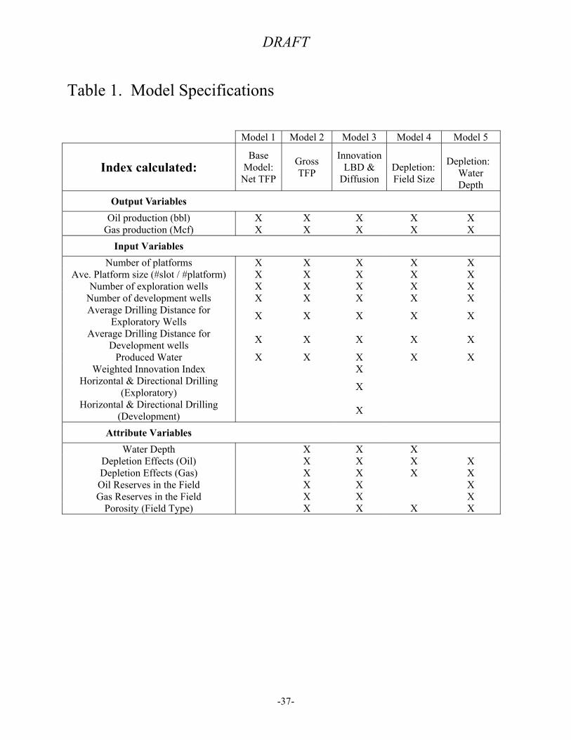
and attribute (a) variables are listed in Table 1. The weighted innovation index at time t is
assigned to vintage group i = t, and hold constant for all field years (j) in that group (i). Besides
the two depletion variables, other attribute variables (e.g., water depth) are constant for each field
(k) in all years. We use cumulative values for inputs (x) and outputs (y), because for the above
technology definition (i.e., x can produce y), it is more appropriate to express the production
relationship on cumulative terms for a nonrenewable industry. For example, for a field, the
production at t is determined by cumulative inputs (e.g., drilling) and outputs (i.e., stock
depletion) up to t-1.
Under Variable Returns to Scale (VRS) following Ray and Desli (1997)5 the Malmquist
index defined above can be decomposed into measures associated with technological change,
efficiency change and scale change:
MTFPVRS = TCVRS · ECVRS · SCVRS.
where TCVRS is technological change under VRS, ECVRS is efficiency change under VRS and
SCVRS is scale change. Technological change measures shifts in the production frontier.
Efficiency change measures changes the position of a production unit relative to the frontier--so-
called “catching up” (Färe et al, 1994). Scale change measures shifts in productivity due to
changes in the scale of operations relative to the optimal scale.
DRAFT
-11-
Each of these measures is indicated in Figure 1. The move from point a to b represents a
change in efficiency, as a production unit moves from an inefficient point, to a point along the
production frontier at time t, Ft(Xt). The associated measure of efficiency change is the ratio of
the distance functions, fb/fa. The movement from point b to point c represents scale change. A
given level of aggregate production can be produced most efficiently if all firms produce at the
optimal scale, where all scale economies are realized but decreasing returns have not yet set in.
This is the point where line for constant returns to scale (CRS), 0g, is tangent to the VRS
production function. The associated measure of scale efficiency is the ratio of distance functions
fg/fb, which is the measure of the scale change for the move from point b to point c, where in
this example scale efficiency is 1 (ec/ec). Finally, technological change is measures shifts in the
production frontier. The measure of technological change associated with a move from point c
to point d is the ratio of the distances ed/ec.
The CRS measure of technological change can be further decomposed into measures of
input biased technological change, output biased technological change and magnitude change:
TCCRS = IBTCCRS · OBTCCRS · MCCRS
where TCCRS is technological change under CRS, IBTCCRS is input-biased technological change
under CRS, OBTCCRS is output-biased technological change under CRS, MCCRS is magnitude
component under CRS, which is the measure of Hicks neutral technological change. Thus, if the
output and input biased measures of technological change are both equal to one, then
technological change is Hicks neutral.
While DEA allows one to quantitatively measure technological change, it does nothing to
alleviate the “confession of ignorance” regarding what constitutes and shapes technological
change. Initially in the innovation literature, data on R&D were used as a proxy for innovation.
DRAFT
-12-
R&D expenditures indicate the effort expended in the search for new technology, and so
provides a measure of inputs to innovation, but R&D expenditures are not a good proxy for
innovation (e.g., Griliches, 1984). Many firms conduct R&D fruitlessly for years, and some
innovative firms create major breakthroughs with little officially recorded R&D. The
measurement issues are especially troublesome for analyses that capitalize on long time series of
data, as the relationship between R&D expenditures and innovation may vary systematically
over time. New innovations may take advantage of past knowledge created (Romer, 1990)
implying an accelerating productivity of R&D expenditures over time. On the other hand, there
may be an ultimate depletion of technological advances over time (Griliches, 1994) implying an
S-shaped relationship between R&D expenditures and innovation. Either of these effects will
impart a bias in R&D expenditure as a measure of technological change with a long time series
of data.
As patent statistics became more rapidly available, patent counts were used as a closer
approximation to innovation (e.g., Schmookler, 1954; Griliches, 1984). However, patent
statistics can be misleading, since many patents never see commercial application, many
innovations are not patented, and some are subdivided into multiple patents, each covering one
or more aspects of the innovation. In response to these issues, refinements of patent counts use
citations as a weight to the patent (see Hall, Jaffe and Trajtenberg, 2001). But changes in patent
policies over time may again make patent counts a misleading measure of innovation,
particularly over long time periods.
Moss (1993) and Cuddington and Moss (2001) provide further refinement of measures of
technological change by counting of the number of innovations each year, as reported in trade
journals. This represents a significant advance, but a simple innovation count treats all
DRAFT
-13-
innovations as having an equivalent impact on productivity. In fact, various new technologies
have different levels of significance, and it is important that these differences are reflected in the
computation of the technology index. A small number of major breakthroughs may have larger
productivity effects than a larger number of incremental innovations. For example, during the
last decade, technologies such as the 3–D seismic modeling have had some of the largest impacts
on productivity and profitability.
Other measures have been taken to identify the importance of innovations, as recognized
by the industry. A study by the National Petroleum Council (NPC) analyzed the needs of the
industry to identify specific advances needed in each technology area and the expected level of
impact of specific technological innovations, both in the short term and the long term (National
Petroleum Council, 1995). The 89 companies who responded to the survey account for about 50
percent of total U.S. reserves. However, the economics literature on technological change has yet
to capitalize on these industry surveys.
We refine available literature on innovations in several ways. First, we modified the
Moss (1993) innovation count index to include production and management technologies, and
updated the index over the full period from 1947–1998. Next, we incorporate the results of the
NPC oil and gas technology surveys with the extended Moss index to construct an importance
weighted innovation index. Details of the methods employed for constructing our refined
technology index are discussed below. We apply these measures within a DEA framework to
measure the impact of identifiable new technologies on productivity change, thereby contributing
to a better understanding of nature of technological change for our application.
DRAFT
-14-
Application of the Model
We measure and decompose productivity change over time in the offshore Gulf of
Mexico oil and gas industry. Production in this nonrenewable resource industry is positively
affected by exploration–development–production efforts, resource stock size and field quality.
As the most easily accessible stocks are depleted, industry must move to fields that are more
remote, smaller and otherwise more expensive to operate. Thus, productivity will decline over
time in the absence of new technologies that ameliorate depletion effects.
Data used in this analysis are obtained from the U.S. Department of the Interior, Minerals
Management Service (MMS), Gulf of Mexico OCS Regional Office. Specifically, we develop
our project database using five MMS data files:
(1) Production data, including monthly oil, gas, and produced water outputs from every well
in the Gulf of Mexico over the period from 1947 to 1998. The data include a total of
5,064,843 observations for 28,946 production wells.
(2) Borehole data describing drilling activity of each of 37,075 wells drilled from 1947 to
1998.
(3) Platform data with information on each of 5,997 platforms, including substructures, from
1947 to 1998.
(4) Field reserve data including oil and gas reserve sizes and discovery year of each of 957
fields from 1947 to 1997.
(5) Reservoir-level porosity information from 1974-2000. This data includes a total of
15,939 porosity measurements from 390 fields.
DRAFT
-15-
Thus, the project database is comprised of well-level data for oil output, gas output,
produced water output, and the quantity of fluid injected, and field-level data for the number of
exploration wells drilled, total drilling depth of exploration wells, total vertical depth of
exploration wells, number of development wells drilled, total drilling distance of development
wells, total vertical distance of development wells, number of platforms, total number of slots,
total number of slots drilled, water depth, oil reserves, gas reserves, original proved oil and gas
combined reserves in BOE, discovery year, and porosity.
Although we have well-level production data, the well level is not a good unit for
measuring technological efficiency due to spillover effects across wells within a given field.
Rather, the field level is a more appropriate unit for measuring technological efficiency. For this
reason, the relevant variables were extracted from these MMS data files and merged by year and
field, so that the final data set was comprised of annual data from 933 fields over a 50-year time
horizon. On average there are 370 fields operating in any particular year, and a total of 18,117
observations.
Output variables in our model are oil production and gas production, while input
variables include number of platforms, platform size, number of development wells, number of
exploration wells, average distance drilled for exploratory wells, average distance drilled for
development wells and untreated produced water6. Field attributes are water depth, initial oil
reserves, initial gas reserves, field porosity, and an aggregate measure of resource depletion,
based on total extraction of oil and gas reserves in the Gulf of Mexico to date for each time
period. Further description of the data is provided in Appendix.
One goal of the study is to measure productivity effects associated with specifically
identifiable new technologies, as compared to productivity effects of less structural means, such
DRAFT
-16-
as learning obtained through experience. Moss (1993) constructs a technology diffusion index
that counts technology diffusion as it is reported in industry trade journals. First, we adapt Moss’
methodology to focus on innovation, rather than diffusion, of technologies and we extend the
index for our full study period, from 1947 to 1998. We modify the Moss index to reflect
innovation by counting only the first time a particular technology is reported, so our index
measures technological innovation rather than diffusion.
Next, we use the impact of needs for each technology in NPC survey as measure of the
significance of different technologies. To do so NPC technologies are allocated to 17 categories
in the simple innovation counts. Technology weights of short and long term significance from
the NPC survey are then used to construct a weighted technology index. The cumulative
weighted technology innovation index at time t is calculated as:
.0 1
,,∑∑= =
×=t
tt
I
iti
NWtit
W InnovwInnov
where InnovWt is the cumulative weighted technology innovation index at time t; wi,t is the
weight for technology in category i at time t; InnovNWi,t is the non-weighted technology
innovation count adapted from Moss in category i at time t.
In addition to this weighted innovation index, one important innovation of the recent
decades is the extent of horizontal and directional drilling. Horizontal drilling refers to the ability
to guide a drillstring to deviate at all angles from vertical, which allows the wellbore to intersect
the reservoir from the side rather from above. This allows a much more efficient extraction of
resources from thin or partly depleted formations. Horizontal drilling is also advantagous for
formations with certain types of natural fractures, low permiability, a gap cap, bottom water, and
for some layered formations. A measure of horizontal & directional drilling7 and our weighted
innovation variable are used in the DEA framework to partition impacts of technological change

DRAFT
-17-
into components associated with specific technological innovations and more routine learning by
doing in the following.
We use several different versions of the model to measure and decompose productivity
changes. First, a base model is used to calculate net productivity change, which measures the net
effect of increases in productivity due to improvements in production technology and declines in
productivity due to depletion. A net technological change index greater than one implies
technological change offsets the depletion effects, while a net technological change index less
than one implies depletion dominates technological change.
Next we decompose net TFP change into decreases in productivity associated with
resource depletion and increases in productivity after accounting for depletion effects:
TFPNet = TFPGross· TFPDepletion,
where TFPNet is the net measure of TFP, which is a measure of the net change in productivity,
including both increases in productivity after accounting for depletion effects (TFPGross) and
decreases in productivity due to depletion (TFPDepletion).
To carry out this decomposition, the second model includes variables that measure
resource depletion: measures of historic resource extraction from the Gulf of Mexico, water
depth, porosity and field size. When these variables are treated as field attributes, DEA calculates
technological change after accounting for changes in these attributes, effectively holding these
depletion variables fixed. The DEA results with this model provide our gross measure of TFP
change, which measures increases in productivity after accounting for depletion effects. The
depletion effect is then calculated as:
TFPDepletion = TFPNet/TFPGross.
DRAFT
-18-
Thus, dividing the net measure of technological change from Model 1 by the gross measure of
technological change from Model 2 provides the measure of the decline in productivity due to
depletion.
Next we decompose the gross measure of technological change into indexes that
represents specific technological innovations and a residual, which we generally term learning by
doing. Thus, the gross index of technological change is decomposed as:
TCGross = TCinnov · TCLBD
where TCGross is the gross index of technological change, TCinnov is the technological change
associated with identifiable new technologies (the weighted innovation index and the measures
of horizontal drilling) and TCLBD is the net index of technological change that cannot be
explained by specifically identifiable new technologies, and includes such factors as learning-by-
doing (Arrow, 1962) and other non-structural factors.
This is accomplished by using the standard DEA decomposition of TFP change into
technological change (TC), or shifts in the production frontier, and efficiency change (EC), or
movements towards (or away from) the frontier. First TFP change from Model 1 is decomposed
into TC and EC using standard DEA methods. This TC component incorporates all forms of
technological change. This is divided by TC, as calculated in Model 3, which includes the
weighted technological innovation index discussed above and the measure of horizontal drilling
treated as “inputs”. Thus, applying DEA to Model 3 calculates an index of technological change
net of specific measurable technological innovations. So Model 3 measures shifts in the
production frontier that cannot be accounted for by specific new innovations, and we generally
term this residual measure of technological change as the result of from learning by doing
(TCLBD). This method allows us to explain a portion of technological change associated with
DRAFT
-19-
specific innovations, and narrow our “confession of ignorance” to the residual effect. Thus, the
fraction of TC associated with specific innovations is:
TCInnov = TCGross/TCLBD
In the same way, we decompose the Efficiency Change (EC) into two indexes. It is
defined ECinnov as Efficiency Change index by DEA with additional input variables InnovWt. EC
as Efficiency Change index without InnovWt. EC is always greater than ECinnov since InnovW
t is
the increasing function of time t. The difference between EC and ECinnov is due to the impact of
InnovWt. Define this effect (EC / ECinnov) as Diffusion index of new technology, DIFF. More
InnovWt explain the efficiency improvement, Diffusion index increases. Diffusion index
measures the catching up effects of inefficient firm or field to the frontier. This implies that more
firms adopt new technologies.
Next, we construct separate measures of the impacts on TFP over time due to reductions
in field size and increases in water depth. Again following methodology described above,
including variable(s) associated with each effect calculates the residual productivity effects after
accounting for changes in the variable(s). The effect of the relevant variable(s) is calculated by
dividing the TFP results of the model excluding the relevant variable(s) by the TFP result of the
model including the variable(s). Model 4 excludes variables that measure field size (initial oil
and gas reserves in the field). So the effect of changes in field size over time is calculated by
dividing the results of the Model 4 by the results of Model 2. Similarly, Model 5 excludes a
variable measuring water depth of the field. So the effect on productivity of changes in water
depth over time is calculated by dividing the results of the Model 5 by the results of Model 2.
Results
DRAFT
-20-
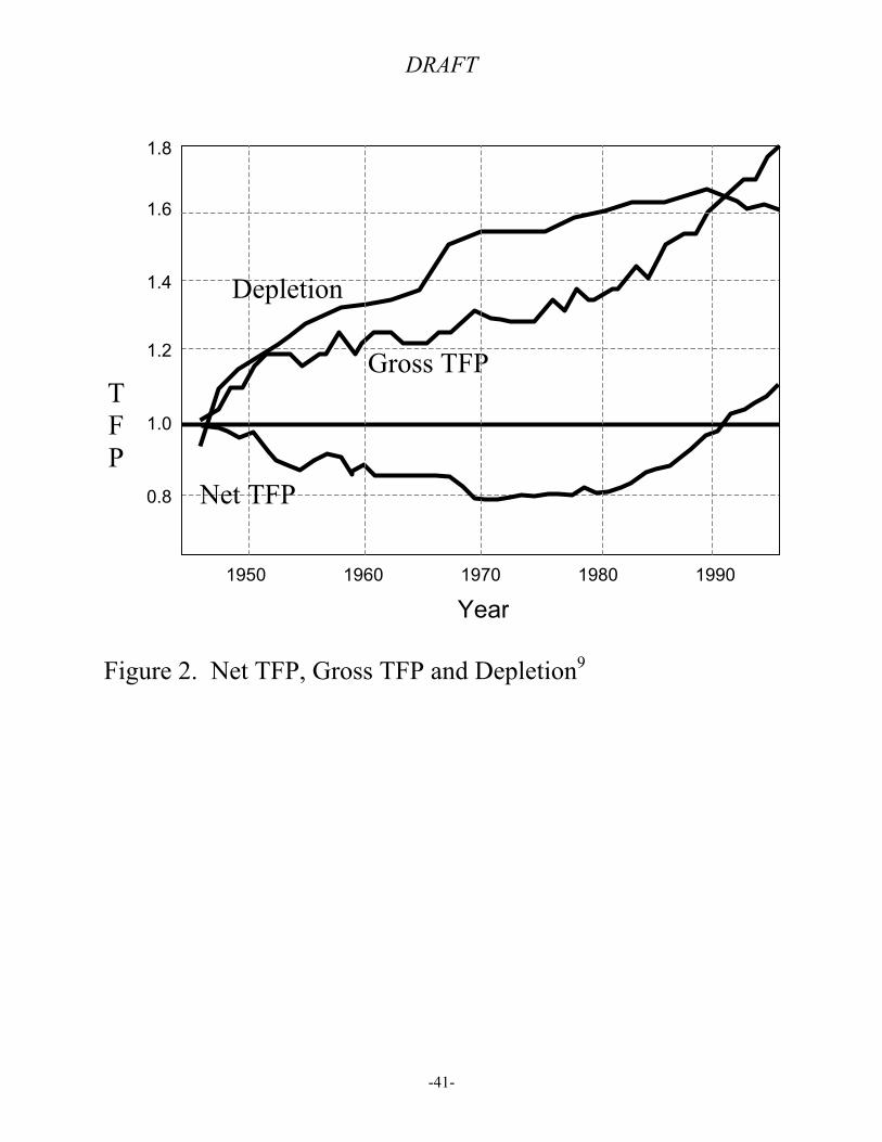
The results for net TFP, gross TFP and depletion effects are presented in Figure 2. Net
TFP declines by about 17 percent from 1947 through 1970, or a rate of about 0.8 percent per
year. Net TFP then remains approximately constant from 1970 through about 1982, increasing
by a total of about 2.5 percent over the period, or about 0.2 percent per year. TFP then increases
by a total of over 33 percent during the remainder of the time horizon, or a geometric average of
about 2.1 percent increase in net TFP per year for the last 15 years of the study period.
Overall, TFP increases by about 10.6 percent over time 50 year study period, for a
geometric mean of about 0.2 percent per year. However, the pattern of TFP change is not
monotonic. Rather, depletion effects initially outweigh productivity enhancing effects of new
technology, but later in the study period technological advance overcomes depletion effects.
This appears contrary to the commonly held notions of uni-directional (increasing or decreasing)
changes in net productivity, or inverted “U” shaped productivity curves (e.g., Slade, 1982),
whereby technology temporarily prevails, eventually to be overwhelmed by physical depletion.
However, the results are consistent with common reports of Gulf of Mexico production,
as discussed above, with the Gulf of Mexico referred to as the “Dead Sea” in the early 1980’s,
and recent reports of technologies that have led to a rapid pace of productivity enhancement
(e.g., Bohi, 1998). This should not, however, be taken as an indication that productivity will
necessarily continue to follow this “U” shaped curve of increasing productivity. Recent years
have seen dramatic improvements in technology that have, to date, offset increasing physical
resource scarcity. It remains to be seen, however, whether we can maintain this pace of
increasing productivity in the near future, or whether recent productivity gains will soon be lost
to depletion, as reserves in deep waters are depleted. Forecasting future trends is always
DRAFT
-21-
dangerous, but it may not be realistic to expect to maintain indefinitely the current accelerating
rate of technological change in offshore production technology.
Fagan (1997) estimated that, holding technology constant, depletion has led to an average
annual increase of 12 percent in the cost of finding new reserves over the period from 1977–94.
Since Fagan estimates that the cost decreasing effects of technological change between 1978 to
1989, depletion effects outweigh the technological change effects over this portion of the study
period. However, Fagan estimates that technological change has outpaced depletion effects in
the period since 1989, so that net TFP increased in the final five years of her study period.
Overall, Fagan finds that TFP is higher in 1994 than it was in 1978.
Together, these results suggest that, after removing effects due to improvements in
technology, both the costs of finding new fields and the cost of producing from fields has been
increasing over time due to depletion effects. But both Fagan’s results on finding costs and our
results on production efficiency show an increasing rate of technological change which offsets
depletion effects over period from 1978 to 1994, and the growth rate in net TFP has been
increasing over time.
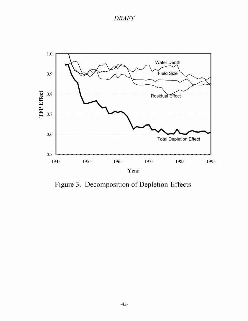
Next we decompose depletion effects into those associated with changes in field size,
water depth, porosity and residual depletion effects, shown in Figure 3. Field size and water
depth appear to have roughly comparable effects on productivity over the study period, but
initially moving to smaller field size appears to have the larger effect, while water depth has a
larger effect on productivity by the end of the study period. This likely has resulted because
production has moved to very great water depths in recent years, with production occurring at
over a mile deep by 1997 and exploratory wells being drilled in nearly 10 thousand feet of water
by 2001. However, deep water production has allowed discovery of larger fields, with recent
DRAFT
-22-
deepwater fields producing at higher rates than has ever been previously achieved in the Gulf of
Mexico. Indeed, by late 1999, more oil was produced by Gulf of Mexico deepwater fields, those
in greater than 1,000 feet of water, than by fields in less than 1,000 feet (U.S. Minerals
Management Service, 2000).
The results of technological change decomposition into output biased technological
change (OBTC), input biased technological change (IBTC) and magnitude change (MC) are
presented in Fig. 4. The magnitude component equals the technological change under joint Hicks
neutrality, when the input biased and output biased components are simultaneously equal to 1
(Färe and Grosskopf, 1996). Our results show that input biased technological change equals 3.60
and output biased technological change equal 2.44, and therefore the biased technological change
index, which is the product of IBTC and OBTC, is 8.78. This bias index is far from one, which is
not consistent with Hicks neutral technological change. Therefore, we reject the assumption of
Hicks neutrality, and technological change is biased both on the input and output sides. The
IBTC is substantially larger than OBTC, reflecting more input efficient use8. In contrast to the
parametric measurement of bias (e.g., Antle and Capalbo 1988), DEA does not provide relative
measures of bias, such as input using or saving with respect to each individual input. Instead
DEA measures the absolute change to assess the extent of input and output biases.
Finally, TFP change in Gulf of Mexico OCS production is decomposed into innovation,
learning by doing and diffusion using the weighted innovation index discussed above. Recall
that we constructed a weighted technology index by extending the Moss innovation-count index
using the NPC survey of importance of technological innovations. In addition, we incorporate a
measure of the use of horizontal drilling technology, as discussed above and in Appendix. Using
these innovation indexes as attributes accounts for the effects of specifically identifiable new

DRAFT
-23-
technologies. The residual component of technological change is then interpreted as a measure
of the non-structural component of technological change, which we generally term “learning-by-
doing” effects.
Figure 5 shows the trends for innovation, learning by doing and diffusion over period
from 1947 through 1995. It shows that the learning-by-doing effect is approximately two times
as large as the affect associated with specific new technological innovations. Over the 49 year
study period, TFP change can be partitioned into 23.9 percent due to innovations, 45.8 percent
due to learning by doing and 46.8 percent due to diffusion. This implies that the contributions to
TFP of learning by doing and diffusion are each approximately double the contribution of
innovation. This implies that although technological innovation is crucial for improving TFP,
there are much more productivity gains from learning by doing and diffusion. Thus shows the
importance of policies that focus on allowing flexibility in operations and that are not overly
restrictive on diffusion of new technologies to other companies.
V. Conclusions
Over time, economists have greatly improved our understanding of the role of
technological change in economic growth and of the constituents of technological change. We
have progressed from “confessions of ignorance” based on mere observations that productivity
increases over time, to an increasingly sophisticated understanding of the mechanisms that drive
technological change and empirical measures of various components of technological change.
This paper contributes to this literature in several ways. First, we use a unique and
extensive micro-level data set to provide a detailed analysis of productivity change at the
production stage of offshore oil and gas. This contributes to our understanding of the extent to

DRAFT
-24-
which technological progress has ameliorated resource depletion in this industry, and thereby the
potential for technological change to fuel continued economic growth in the face of fixed stocks
of non-renewable resources. Our unique data set also allows us to decompose productivity
change into various constituents, which provides a more detailed understanding of the nature of
productivity change for this important industry.
We apply Data Envelopment analysis (DEA) techniques (e.g., Charnes et al, 1978; Färe
et al., 1985) to a unique field-level data set to measure the extent to which technological change
offsets resource depletion effects. Our results show that increases in productivity have offset
depletion effects in the Gulf of Mexico offshore oil and gas industry over 49 year period from
1947-1996. However, the nature of the effect differs significantly from what is typically
assumed for non-renewable resource industries. During the first 30 years of the time horizon, we
found productivity declines in offshore oil and gas production. But in more recent years, net
productivity increased, offsetting depletion effects. Productivity change has been highest in the
past 5 years, indicating that we may still be along the increasing portion of the “S” shaped
technological time path. However, extrapolating trends into the future is risky, especially over
longer time periods. It could well be that the pace of technological advance could slow in the
near future, and depletion effects could lead to rapid declines in productivity in this important
non-renewable resource industry.
We decomposed depletion effects into effects associated with changes in field size, water
depth, porosity and a residual that measures aggregate resource extraction in the Gulf of Mexico.
We found that each of these effects are roughly similar in magnitude, that that interesting shifts
occur over time. For example, initially field size appeared to be more important than water
depth. However, as new technologies allowed us to find larger fields by moving to ever deeper
DRAFT
-25-
waters, water depth tended to have a stronger effect on reducing TFP than did field size. Once
again, it remains to be seen whether this trend will continue, or whether we will quickly deplete
the stock of large, deep water fields.
We also analyzed the contribution of technological change and efficiency change in
sector total factor productivity (TFP). The former comprises technological innovation and
learning by doing, and the latter technology diffusion and other factors. We developed an index
for decomposing technological change into technological innovation and learning by doing, and
we estimated the relative importance of technological innovation, learning by doing and
technology diffusion on TFP. Similarly, we isolated technology diffusion from that the rest of
the factors that impact on efficiency change and subsequently TFP. We compared the relative
impact of these technology indicators on TFP in the industry. The results indicate that both
learning by doing and diffusion of technological had a significantly larger impact on TFP than
technological innovation. This implies that although technological innovation is crucial for
improving TFP, there are even much more productivity gains from learning by doing (experience
of engineers and mangers) and adoption of new technology in the offshore oil and gas industry.
This suggests the importance of developing policies that provide flexibility in implementing
available technologies.
DRAFT
-26-
Appendix: Data
A.1. Data Construction
Data used in this analysis are obtained from the U.S. Department of the Interior,
Minerials Management Service (MMS), Gulf of Mexico OCS Regional Office. We develop our
project database using five MMS data files:
(1) Production data including well-level monthly oil, gas, and produced water outputs from
1947 to 1998. The data include a total of 5,064,843 observations for 28,946 production
wells.
(2) Borehole data describing drilling activity of each of 37,075 wells drilled from 1947 to
1998.
(3) Platform data with information on each of 5,997 platforms, including substructures, from
1947 to 1998.
(4) Field reserve data including oil and gas reserve sizes and discovery year of each of 957
fields from 1947 to 1997.
(5) Maximum efficiency rate data including reservoir-level porosity information from 1974-
2000. The data include porosity information for 390 fields and has a total of 15,939
observations.
Relevant variables are extracted from these MMS data files and merged by year and field. Using
these variables, the Gulf of Mexico regional new resource discovery and depletion over time are
constructed. The variable for horizontal & directional drilling is defined as the ratio of total
drilling distance to vertical drilling depth. Larger values imply a higher ratio of horizontal &
DRAFT
-27-
directional drilling relative to vertical drilling. We take cumulative input value data, as literature in
the oil and gas supply suggest (e.g., Pindyck, 1978b), for well, drilling, horizontal & directional
drilling. Drilling is assumed to affect output starting the following year, since current drilling does
not affect current production. So well inputs in period t are determined by cumulative drilling
through period t-1. At any point in time ultimately recoverable resources are not known. Rather, the
remaining resource is estimated using current economically (not physically) known reserve stock
minus resources produced to date. We also take cumulative value for output variables including oil,
gas production to take account of the technological characteristics.
An aggregate depletion effect is measured using a measure of remaining resource of oil and
gas separately in whole Gulf of Mexico on period t–1. We aggregate the production data both for
oil and gas separately over fields, and we next calculate the cumulative value over time. The
depletion measure is [1– (cumulative until (t–1) period) / (cumulative until 1995)]. This captures the
effect how much resource is extracted already in each period.
DEA requires the data on input usage and on characteristics that determine output. We
created the water depth (in feet) attribute as maximum water depth in the Gulf of Mexico minus
water depth in each field, since production is more difficult in deeper water depth in given
technology. Units of oil and gas production are barrels and thousand cubic feet, respectively.
Platform size is defined as average number of slots per platform for the field. Units of oil and gas
reserves are million barrel and billion cubic feet, respectively. Units of remaining oil and gas
reserves in the Gulf of Mexico, and porosity are measured in percent terms. More precise
description of data is in Managi (2001).

DRAFT
-28-
A.2. Missing Data Estimation
Complete data for porosity is available for 390 fields out of 933 fields. We use two-step
estimation procedure to correct for this omitted variable problem (Heckman 1979; Greene 1981).
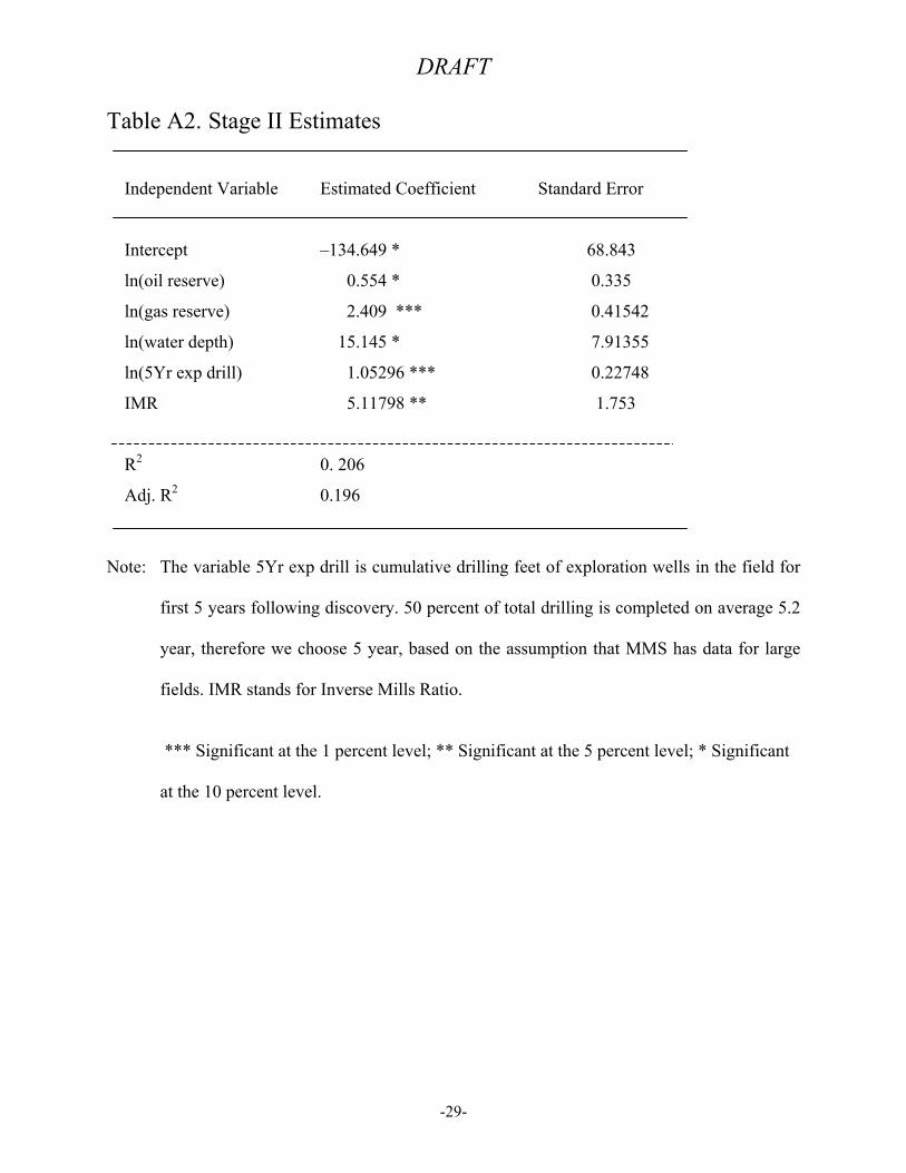
Table A. 1 and A.2 contains estimation results from these regression models. Results for second
step as OLS in Table A.2 imply that higher porosity values tend to be found in larger reservoirs,
in reservoirs in which more drilling occurs and in deeper-water fields.
Table A1. Stage I Probit Estimates
Independent Variable Estimated Coefficient Standard Error
Intercept 811.234 *** 65.866
Discovery Year –106.926 *** 8.679
Log Likelihood –543.8820313
Note: Dependent variable = 1 if porosity observed; 0 otherwise. *** Significant at the 1 percent
level.
DRAFT
-29-
Table A2. Stage II Estimates
Independent Variable Estimated Coefficient Standard Error
Intercept –134.649 * 68.843
ln(oil reserve) 0.554 * 0.335
ln(gas reserve) 2.409 *** 0.41542
ln(water depth) 15.145 * 7.91355
ln(5Yr exp drill) 1.05296 *** 0.22748
IMR 5.11798 ** 1.753
R2 0. 206
Adj. R2 0.196
Note: The variable 5Yr exp drill is cumulative drilling feet of exploration wells in the field for
first 5 years following discovery. 50 percent of total drilling is completed on average 5.2
year, therefore we choose 5 year, based on the assumption that MMS has data for large
fields. IMR stands for Inverse Mills Ratio.
*** Significant at the 1 percent level; ** Significant at the 5 percent level; * Significant
at the 10 percent level.
DRAFT
-30-
References
Aghion, Philippe and Howitt, Peter. 1992, A Model of Growth through Creative Destruction.
Econometrica 60 (2): 323-51.
Alchain, A., 1963, Reliability of Progress Curves in Airframe Production. Econometrica 31:
679-693.
Antle, John M., and Capalbo, Susan M. An Introduction to Recent Developments in Production
Theory and Productivity Measurement, in Capalbo, Susan M.; Antle, John M., eds., 1988,
Agricultural Productivity: Measurement and Explanation. Washington, D.C.: Resources
for the Future; Distributed by the Johns Hopkins University Press.
Arrow, Kenneth J. 1962, The Economic Implications of Learning by Doing. Review of Economic
Studies 29:155-73.
Baumol, W.J., Oates, W.E. 1988, The Theory of Environmental Policy, 2nd edition, Cambridge:
Cambridge University Press.
Barbier, Edward B, 1999, Endogenous Growth and Natural Resource Scarcity, Environmental
and Resource Economics 14 (1): 51-74.
DRAFT
-31-
Barnett, Harold and Morse, Chandler, 1963, Scarcity and Growth, Baltimore: Johns Hopkins
Press.
Barro, R. J. and Sala-i-Martin, X., 1995. Economic Growth. New York, McGraw-Hill.
Berck, Peter and Roberts, Michael, 1996. Natural Resource Prices: Will They Ever Turn Up?
Journal of Environmental Economics and Management 31 (1): 65-78.
Bohi, Douglas R., 1998 Changing Productivity in U.S. Petroleum Exploration and Development.
Resources for the Future, Discussion Paper 98-38.
Boulding, Kenneth E., 1966, The Economics of the Coming Spaceship Earth. in H. Jarrett. eds.,
Environmental Quality in a Growing Economy, pp. 3-14. Baltimore, MD: Resources for
the Future/Johns Hopkins University Press.
Caves, Douglas W, Laurits R. Christensen and W. Erwin Diewert, 1982a. Multilateral
Comparisons of Output, Input and Productivity Using Superlative Index Numbers.
Economic Journal 92 (365): 73-86.
Caves, Douglas W, Laurits R. Christensen and W. Erwin Diewert, 1982b. The Economic Theory
of Index Numbers and the Measurement of Input, Output and Productivity. Econometrica
50(6): 1393-1414.

DRAFT
-32-
Charnes, A., Cooper, W. W. and Rhodes, E., 1978. Measuring the Efficiency of Decision
Making Units. European Journal of Operational Research 2(6): 429-444.
Cleveland, Cutler J; Kaufmann, Robert K, 1997, Natural Gas in the U.S.: How Far Can
Technology Stretch the Resource Base? Energy Journal 18 (2): 89-108.
Cole, H.S.D, Christopher Freeman, Marle Jahoda and K.L.R. Pavitt, 1975. Models of Doom: A
Critique of the Limits to Growth, New York: University Books.
Cropper, Maureen L; Oates, Wallace E, 1992, Environmental Economics: A Survey. Journal of
Economic Literature 30 (2): 675-740.
Cuddington, J.T., and Moss, D. L. 2001. Technical change, depletion and the U.S. petroleum
industry: a new approach to measurement and estimation. American Economic Review
91(4): 1135-1148.
Daly, Herman E., 1991. Steady-State Economics, Island Press: Washington, D.C.
Deffeyes, Kenneth S., 2001. Hubbert’s Peak: The Impending World Oil Shortage. Princeton
University Press.
Fagan, Marie N, 1997. Resource Depletion and Technical Change: Effects on U.S. Crude Oil
Finding Costs from 1977 to 1994. Energy Journal 18 (4): 91-105.
DRAFT
-33-
Färe, R., Grosskopf S., 1996, Intertemporal Production Frontiers, Kluwer-Nijhoff Publishing,
Boston.
Färe, R., Grosskopf, S., and Lovell, C.A. Knox, 1985. The Measurement of Efficiency of
Production. Boston: Kluwer-Nijhoff.
Färe, R., Grosskopf, S., Norris, M., Zhang, Z., 1994. Productivity Growth, Technical Progress,
and Efficiency Change in Industrialized Countries. American Economic Review 84(1):
66–83.
Greene, William. 1981, Sample Selection Bias as a Specification Error: Comment,
Econometrica 49(3) 795-98.
Griliches, Zvi, ed, 1984. R&D, Patents, and Productivity, NBER Conference Report. Chicago
and London: University of Chicago Press.
Griliches, Zvi, 1994. Productivity, R&D and the Data Constraint. American Economic Review
84(1): 1-23.
Hall, Bronwyn H., Jaffe, Adam B., Trajtenberg, M., 2001. The NBER Patent Citations Data File:
Lessons, Insights and Methodological Tools. NBER Working Paper No. W8498.
DRAFT
-34-
Heckman, James. 1979. Sample Selection Bias as a Specification Error. Econometrica 47(1):
153-161.
Jin. D, Kite-Powell, H., and Schumacher, M.. 1998, Total Factor Productivity Change in the
Offshore Oil and Gas Industry. Woods Hole Oceanographic Institution Working Paper.
Malmquist, S. 1953, Index Numbers and Indifference Curves. Trabajos de Estatistica, 4 (1):
209-42.
Malthus, Thomas, 1826. An Essay on Population, London: Ward, Lock and Company.
Managi, Shunsuke, forthcoming. Technological Change, Resource Depletion and Environmental
Policy in Offshore Oil and Gas Industry. Ph.D. dissertation, University of Rhode Island.
Meadows, Donella H., Dennis L. Meadows, Jorgen Randers, and William W. Behrens III, 1972.
The Limits to Growth, New York: Potomac Associates.
Moss D. L. 1993, Measuring Technical Change in the Petroleum Industry: A New Approach to
Assessing its Effect on Exploration and Development. National Economic Research
Associations, Working Paper #20.
National Petroleum Council, 1995. Research Development and Demonstration Needs of the Oil
and Gas Industry. Washington, D.C.
DRAFT
-35-
Pindyck, R.S. 1978a, Higher Energy Prices and the Supply of Natural Gas. Energy Systems and
Policy 2 (2): 177-207.
Pindyck, R.S. 1978b. The Optimal Exploration and Production of Nonrenewable Resources.
Journal of Political Economy 86 (5): 841-861.
Ray, Subhash C; Desli, Evangelia, 1997, Productivity Growth, Technical Progress, and
Efficiency Change in Industrialized Countries: Comment. American Economic Review 87
(5): 1033-39.
Romer, Paul M. 1990: Endogenous Technological Change. Journal of Political Economy 98 (5,
pt. 2): S71-S102.
Schmookler, Jacob, 1954, The Level of Inventive Activity, Review of Economics and Statistics
36(2):183-190.
Slade, M. 1982 Trends in Natural-Resource Commodity Prices: An Analysis of the Time
Domain. Journal of Environmental Economics and Management 9(2): 122-137.
Stiglitz, Joseph E, 1974, Growth with Exhaustible Natural Resources: Efficient and Optimal
Growth Paths, Review of Economic Studies 0, Symposium, 123-37.
DRAFT
-36-
U.S. Department of Interior, 2001. Technical Information Management System (TIMS)
Database, U.S. Mineral Management Service (MMS).
U.S. Minerals Management Service, 2000. Deepwater Gulf of Mexico: America’s Emerging
Frontier. OCS Report 2000-022.
U.S. Minerals Management Service, 2000. Mineral Revenue Collections.
Young, Alwyn, 1993, Invention and Bounded Learning by Doing. Journal of Political Economy
101 (3): 443-72
Walls, M.A. 1994, Using a 'Hybrid' Approach to Model Oil and Gas Supply: A Case Study of the
Gulf of Mexico Outer Continental Shelf. Land Economics 70 (1): 1-19.
Zimmerman, Martin B, 1982, Learning Effects and the Commercialization of New Energy
Technologies: The Case of Nuclear Power. Bell Journal of Economics 13 (2): 297-310.
DRAFT
-37-
Table 1. Model Specifications
Model 1 Model 2 Model 3 Model 4 Model 5
Index calculated:Base
Model:Net TFP
GrossTFP
InnovationLBD &
DiffusionDepletion:Field Size
Depletion:WaterDepth
Output VariablesOil production (bbl) X X X X X
Gas production (Mcf) X X X X XInput Variables
Number of platforms X X X X XAve. Platform size (#slot / #platform) X X X X X
Number of exploration wells X X X X XNumber of development wells X X X X XAverage Drilling Distance for
Exploratory Wells X X X X X
Average Drilling Distance forDevelopment wells X X X X X
Produced Water X X X X XWeighted Innovation Index X
Horizontal & Directional Drilling(Exploratory) X
Horizontal & Directional Drilling(Development) X
Attribute VariablesWater Depth X X X
Depletion Effects (Oil) X X X XDepletion Effects (Gas) X X X XOil Reserves in the Field X X XGas Reserves in the Field X X X
Porosity (Field Type) X X X X

DRAFT
-38-

DRAFT
-39-
Figure 1. Components of Productivity Change withVariable Returns to Scale
f
Ft(X)
Ft+1(X)
a
c
b
d
EfficiencyChange
ScaleChange
TechnologicalChange
Output
Input
0e
g
X

DRAFT
-40-
DRAFT
-41-
Figure 2. Net TFP, Gross TFP and Depletion9
Gross TFP
1.0
0.8
1.2
1.4
19901980197019601950
TFP
Year
1.6
1.8
Net TFP
Depletion
DRAFT
-42-
Figure 3. Decomposition of Depletion Effects
0.5
0.6
0.7
0.8
0.9
1.0
1945 1955 1965 1975 1985 1995
Year
TFP
Eff
ect
Figure 3. Decomposition of Depletion Effects
Total Depletion Effect
Residual Effect
Water Depth
Field Size

DRAFT
-43-
Figure 4. Decomposition of Depletion Effects
0
1
2
3
4
1945 1955 1965 1975 1985 1995
Year
Bia
sed
TC
IBTC
OBTC
MC

DRAFT
-44-
Figure 5. Innovation, Learning by Doing and Diffusion
1
1.1
1.2
1.3
1.4
1.5
1945 1955 1965 1975 1985 1995
DIFF
INNOV
LBD
TC
Year
DRAFT
-45-
Footnotes
1 We define resource depletion broadly to include changes in resource quality (e.g., field size and porosity) and
location (e.g., water depth).
2 Note that Walls’ analysis uses data from 1970 to 1988, with production predicted to decline monotonically over
the forecast period from 1989 though 2000. In actuality, oil production from federal OCS waters increased over
that entire period, and oil production in federal OCS waters in the year 2000 was approximately 2/3rds higher
than in the 1988.
3 Examples of cases where learning by doing has lead to significant cost reductions can be found in Alchain
(1963) and Zimmerman (1982).
4 Although Young (1993) use the word invention instead of innovation, his definition is same as our definition of
innovation.
5 Ray and Desli (1997) argue that MTFP index is equivalent to the ratio of the CRS distance function even if the
technology is not characterized by CRS. Productivity is a long run problem thus it is measured relative to the
CRS technology. In other words, MTFP index under CRS equals the MTFP index under VRS.
6 We follow the usual convention in environmental economics of treating pollution emissions as an input to
production (e.g., Baumol and Oates, 1988; Cropper and Oates, 1992). Thus, a reduction (increase) in untreated
produced water, with all other inputs and outputs held fixed, represents an increase (decrease) in productivity.
7 Appendix A describes the method used for calculating the measure of horizontal and directional drilling.
8 This is consistent with the observation that less wells are drilled from fewer large platforms, resulting from
technological innovations such as 3-D seismology, horizontal drilling, and large deep water platform.
9 Note: The depletion effect is shown in inverted (1/Depletion) in this Figure to more clearly demonstrate the
relative sizes of depletion and gross technological change.