ERIA-DP-2020-09

ERIA Discussion Paper Series

No. 336

Technological Advancement, Import Penetration, and Labour Markets:

Evidence from Thai Manufacturing

Juthathip JONGWANICH,**

Archanun KOHPAIBOON

Faculty of Economics, Thammasat University

Ayako OBASHI

School of International Politics, Economics and Communication

Aoyama Gakuin University

August 2020

Abstract: This paper examines the impacts of advanced technology on a possible change in

workers’ skills, wages, and employment due to such technological advancement. Three proxies

of advanced technologies are used in the study: (i) information and communications

technology, (ii) intensity of robot use, and (iii) value of e-commerce. Our study compares the

effects of technological advancements on labour market outcomes with import penetration,

delineating into raw materials, capital goods, and final products. Our results show that in

Thailand, the impact of advanced technology in pushing workers out of the job market is

limited. Instead, it tends to affect reallocation of workers between skilled and unskilled

positions. The results vary amongst proxies of technology and sectors. It seems that workers

in comparatively capital-intensive industries, including automotive, plastics and chemicals,

and electronics and machinery, are the most affected by advanced technology. Dampened

wage/income is found only in some proxies of technology and sectors. Our results show less

concern of negative impacts induced by imports, particularly imports of capital goods and raw

materials, on employment status and income than technological advancement.

Keywords: Technological advancement, import penetration, labour markets

JEL Classification: F16, O30, O53

Corresponding author. Juthathip Jongwanich, address: Faculty of Economics, Thammasat University, 2 Prachan

Rd., Bangkok 10200 Thailand. ** The authors would like to thank the participants of the first and second workshops on 22 March 2019 and on 9

March 2020 (e-meeting) for their comments. Special thanks are extended to Bin Ni, Fukunari Kimura, Doan Thi

Thanh Ha, Rashesh Shrestha, and Hongyong Zhang. The workshops were arranged in Jakarta, Indonesia by the

Economic Research Institute for ASEAN and East Asia, who also funded the research.

2

1. Introduction

There is a long history of industries being revolutionised by waves of new technology.

Clearly, the world is experiencing the Fourth Industrial Revolution that allows innovation

invented in the three previous industrial revolutions connect to each other. This fourth

revolution has witnessed major advances in technology, which will likely transform the

structure and dynamics of many industries. Industry 4.0 is the next wave of digital and online

transformation as industries are changed through, for example, further automation, artificial

intelligence, robotics, cloud computing, 3D printing, big data analytics, and Internet of Things.

The advancing technologies tend to enable and facilitate a broad range of business activities

related to the storage, processing, distribution, transmission, and reproduction of information.

However, there are concerns about the impacts of advancing technologies on economic

development in both developed and developing countries, especially on labour market

outcome. With such advancing technologies, a wide range of job tasks in many sectors and in

many countries would be fully or partially automated, recently including one considered as

non-routine tasks, e.g. diagnosing disease from X-rays, picking orders in a warehouse, or

driving cars (Bessen et al., 2019). Frey and Osborne (2017) and Ford (2015) argued that the

pace of technological advancements, especially in terms of automation, artificial intelligence,

and robotics, would be accelerating both in developed and developing countries, and the range

of jobs affected by such technologies would be widening. Autor et al. (2003), Acemoglu and

Autor (2011), and Acemoglu and Restrepo (2018b) developed a theoretical model showing

that, with a task-based approach where the central unit of production is task whilst labour and

capital have comparative advantages in different tasks, automation can create displacement

effects resulting in a decline in the demand for labour and wage rate.

Interestingly, so far empirical studies on the impacts of advanced technology on labour

market outcomes, which are mostly based on developed countries, are mixed. On the one hand,

Cirera and Sabetti (2019), Crespi et al. (2019), Hou et al. (2019), Mairesse and Wu (2019),

and Calvino (2019), using outcome measures from technological advancements, showed that,

to some extent, technological advancements help create product innovation and improve

labour market outcomes, including employment and productivity. Bartel et al. (2007), studying

the impacts of new information technologies (IT), revealed that the adoption of new IT

supports skilled workers whilst improving efficiency of all stages of production process. On

the other hand, Arntz et al. (2016), Gaggl and Wright (2017), Acemoglu and Restrepo (2017),

and Bessen et al. (2019) showed threats from technological advancements. Gaggl and Wright

(2017) disclosed that non-routine, cognitive tasks are affected by the adoption of information

and communications technology (ICT); however, there is only modest impact of ICT replacing

3

routine, cognitive work. Acemoglu and Restrepo (2017) showed the negative effects of robots

on employment and wages across commuting zones in the United States (US). Bessen et al.

(2019) pointed out that automation decreases the probability of day works but not wage rate.

With unclear impacts of advanced technology on labour market outcomes, this study

aims to examine such impacts on the labour market of developing countries, like the Thai

labour market during 2012–2017 as a case study. This study contributes to the existing

literature in three ways. First, whilst previous studies analysed the impacts of advanced

technology on labour market outcomes, either employment levels or wage or both, this study

examines a possible change in skills and wages of workers that could be induced by

technological advancements, and the possibility of employed workers becoming unemployed

due to such technological changes. Our analysis used both whole data set of the manufacturing

sector and an individual sector. Autor and Salomons (2018) argued that advanced technology

may only reallocate employment but will not depress overall demand for labour. In addition,

to confirm the effects of technological advancement on wage and income, the wage equation

is applied among workers over time using information of the whole manufacturing sector and

individual sector.

Second, this is different from other studies in the sense that technological advancements

are proxied by three key aspects according to their involvement in supply chains, i.e. inbound

(automated e-sourcing), outbound (e-commerce), and internal production (e.g. factory

automation/robots) (UNCTAD, 2017) to delineate the relative important effects of technology

involvements in supply chains. ICT use and the value of e-commerce in the industry are

utilised to capture possible technological involvements in inbound and outbound activities.

Robots are used in industries to capture the possible impacts of technological advancements

in internal production. Third, since trade, particularly import penetration, is another paramount

force shaping the labour market, this study compares the effects of technological

advancements on labour market outcomes with import penetration. Only a few studies – such

as those of Autor et al. (2015) and Acemoglu and Restrepo (2017) – compared the effects of

two forces, but their works still concentrated only on developed countries. In addition, whilst

previous studies examined the impacts of penetration in terms of total imports, this study

investigates penetration from the perspectives of finished products, capital, and raw materials.

The rest of the paper is structured as follows. Section 2 provides a literature survey on

the impacts of technological advancements on the labour market. Section 3 presents policy

changes towards Industry 4.0 in Thailand and how technology has progressed so far in the

country. Section 4 discusses the empirical model and data sources whilst Section 5 shows the

empirical results. The last section concludes with key findings and provides policy inferences.

4

2. Literature Survey

There is a long history of industries being revolutionised by waves of new technology.

With advancing technologies, there are concerns about their impacts on economic

development in both developed and developing countries, especially on labour market

outcomes. However, studies about such impacts are mixed. On the one hand, some studies

showed that technological advancements, to some extent, help improve labour market

outcomes. For example, Beaudry et al. (2006) examined the impacts of technology adoption

on city-level outcomes, mainly focusing on abundance of skilled labour and wages during

1980–2000. Skilled labour refers to workers who have at least some college education.

Technology adoption is measured by personal computer (PC) intensity, PCs per employee of

each city. Cities that aggressively adopt PCs have a relative abundance of skilled labour and

witness the significant increase in relative wages. Bartel et al. (2007) studied the impacts of

new IT on productivity and worker skills of valve manufacturing during 1999–2003. The

results showed that adoption of new IT supports skilled workers whilst improving efficiency

in all stages of the production process. Meanwhile, the adoption of new IT helps shift from

mass production to more customised valve products.

Cirera and Sabetti (2019) studied the impacts of innovation on employment in 53

developing countries in 2013–2015. Innovation in this study is examined in terms of outcome

measures, i.e. either product, process, or organisation innovation. The study applied that of

Harrison et al. (2014) as a base model where the two types of products – old and new – can

generate demand corresponding to those products. Using a cross-sectional analysis of both

manufacturing and services, they showed that product innovation increases employment, and

the effect is more than job losses due to cannibalisation of old products, particularly in the

high-tech manufacturing sector. The impact of process and organisational innovations on

employment seems negligible. Graetz and Michaels (2018) examined the implications of the

use of robots on labour productivity, total factor productivity, output prices, and employment

in 1993–2007 for 17 countries. The results showed that robot use contributes positively to

labour and factor productivity growth thereby lowering output prices. Robots have

insignificant effects on employment across a panel of countries and industries, but they reduce

the employment share of low-skilled workers. Dauth et al. (2018) found the positive impact of

robotics on wage and no impact on total employment.

Crespi et al. (2019), Hou et al. (2019), and Mairesse and Wu (2019) also applied the

model based on Harrison et al. (2014) in examining the impacts of innovation on employment.

Crespi et al. (2019) used the model for Chile, Uruguay, Costa Rica, and Argentina during

1995–2012 whilst Hou et al. (2019) applied that for the countries of the European Union and

5

China in 1999–2006 and Mairesse and Wu (2019) for China in 1999–2006. Note that Mairesse

and Wu (2019) extended Harrison et al. (2014) by splitting output into domestic and exports,

both of which are decomposed further into new and old products. The results of these three

papers resembled those of Cirera and Sabetti (2019). Calvino (2019) applied different

underlying theories of production and competition for Spain during 2004–2012 in examining

the impact of innovation on employment. As in the previous studies, product innovation

positively affects employment growth of both fast-growing and shrinking firms. However, the

effect of process innovation on employment is insignificant, except in new production methods

or auxiliary processes such as IT, which could stimulate employment growth at the lower end

of its conditional distribution. Barbieri et al. (2019) used different underlying theories of

production and competition for Italy during 1998–2010. However, instead of using outcome

measures for innovation, they used input measures, i.e. research and development and

innovation expenditure, to represent innovation. Innovation tends to have a positive – though

the magnitude is rather small – impact on employment.

On the other hand, several empirical studies found negative impacts of technological

advancements on labour market outcomes. Arntz et al. (2016), for example, followed an

occupation-based approach proposed by Frey and Osborne (2013) but considered the

heterogeneity of workers’ tasks within occupations to determine the risk of automation for

jobs in 21 countries of the Organisation for Economic Co-operation and Development

(OECD). On average, the threat from technological advances seemed to exist but the results

differed across OECD countries. Gaggl and Wright (2017) studied the effect of ICT adoption

on employment and wage distribution. ICT adoption is proxied by the number of workers

using a PC and the number of PCs in the workplace. The result showed that the adoption of

ICT affects non-routine, cognitive tasks whilst it only modestly impacts the replacement of

routine, cognitive work.

Bessen et al. (2019) estimated the impact of automation on individual workers by using

Dutch microdata – and all are in private non-financial industries – in 2000–2016. Direct

measures of automation at the firm level – i.e. automation costs defined as costs of third-party

automation services, including non-activated purchases of custom software and costs of new

software releases – are employed in the study. The paper showed that automation decreases

the probability of day works, which leads to a 5-year cumulative wage income loss of about

8% of 1 year’s earnings, but wage rates are not significantly affected by automation. The

impacts of automation are more gradual and displace far fewer workers than mass layoffs.

Frey and Osborne (2017) examined the impacts of future computerisation on US labour market

outcomes, composed of wages and educational attainment. They applied a Gaussian process

6

to estimate the probability of computerisation for 702 detailed occupations. The author showed

that around 47% of total US jobs has a high probability of being computerised, especially those

in transportation, logistics, and office and administrative support. Wages and educational

attainment exhibit a strong negative relationship with the probability of computerisation.

Acemoglu and Restrepo (2017) examined the impacts of industrial robots on

employment and wages in the US during 1990–2007 on the US local labour market. They used

a model in which robots compete against human labour in producing different tasks. The

results showed that robots negatively affect jobs and wages across commuting zones.

However, the negative impact arising from robots is relatively smaller due to the relatively

few robots in the US economy at that time. Acemoglu and Restrepo (2017) argued that if

robots were used widely in the future, the aggregate implications could be much more sizeable.

Autor et al. (2017) assessed the fall in labour share based on the rise of superstar firms. They

applied US Economic Census data for 3 decades during 1982–2012. The results showed that

industries where concentration rises most tend to have the largest decline in labour share. If

technological changes advantage the most productive firms in each industry, product market

concentration increases from the dominance of superstar firms thereby reducing aggregate

labour share. Autor et al. (2017) showed that the fall in the labour share is driven mainly by

firm reallocation rather than a fall in labour share within firms; this occurs greatly in sectors

with increased market concentration.

However, some studies arguing the impacts of technological advancements on labour

market were unclear, depending on conditions in labour markets and production structure.

Acemoglu and Restrepo (2018a, 2018b, 2019) developed a conceptual framework to

understand how machines replace human labour and how jobs and wages are affected. In such

task-based framework, automation is modelled as the expansion of the set of tasks that can be

performed by capital and can replace labour. In addition to automation, the model introduces

another type of technological change that leads to more complex tasks than existing ones. It is

assumed that labour tends to have more comparative advantage in these new tasks than

automation. In the short run, a displacement effect in which automation can replace labour

could occur thereby depressing demand for labour and wages. However, in the long run, since

labour has a comparative advantage over automation, if the creation of new tasks continues,

employment and labour share can remain stable even in the face of rapid automation.

Acemoglu and Restrepo (2018b) clearly argued that the presence of a displacement effect may

eventually not reduce demand for labour due to three channels, namely, productivity channel,

capital accumulation, and expansion of automation. Yet, Acemoglu and Restrepo (2019)

illustrated productivity improvement in non-automated tasks induced by automation

7

technology, and in which technology creates new tasks reinstating labour into a broader range

of tasks that could counterbalance the displacement effect.

Autor and Salomons (2018) examined the impact of technological progress on aggregate

employment and labour share at the industry-level by considering both direct and indirect

effects. They argued that technological innovations replace workers with machines. But

aggregate labour demand may not be reduced from such capital–labour substitution. Three

countervailing responses could occur to eventually stimulate more demand – including inter-

industry demand linkages and between-industry compositional changes – and increase final

demand. The harmonised cross-country and cross-industry data covering 19 countries of the

Organisation for Economic Co-operation and Development (OECD) during 1970–2007 were

used. They showed that automation directly displaces employment and reduces labour’s share

of value added in the industries. However, there is another effect from inter-industry demand

linkages and final demand countering employment displacement. There is no evidence of

indirect effect in countering the negative impact of the aggregate fall in the labour share. Dauth

et al. (2018), using data from Germany’s labour market in 1994–2014, showed that job losses

induced by robot adoption in the manufacturing sector were offset by gains in the business

service sector. This study also looked at the impacts of robots on individual workers and

showed that risks arising from the displacement effect were minimal for incumbent

manufacturing workers but high for young labour market entrants. The incumbent

manufacturing workers tended to either stay with their original employer or switch occupations

at their original workplace.

Interestingly, few studies – such as Autor et al. (2015) and Acemoglu and Restrepo

(2017) – compared the impacts of technological advancements with those of imports. In fact,

recently both technology and trade were set as two important sources shaping labour markets,

especially in developed countries. For trade, Autor et al. (2015) argued that trade with lower-

wage countries tends to depress wages and employment in industries, occupations, and

regions, exposing import penetration They examined the impacts of technological change

and trade on the US labour market within 722 commuting zones. The results showed that trade

competition, especially from Chinese imports, leads to noticeable declines in manufacturing

jobs in all major occupation groups, including managerial, professional, and technical jobs.

Particularly, workers without a college education are greatly affected. The impact of

technological changes seems to be negligible on overall employment. However, the changes

create substantial shifts in occupational composition within sectors – from routine task–

intensive production and clerical occupations to manual task–intensive occupations.

Acemoglu and Restrepo (2017), as mentioned, also supported the findings of Autor et al.

8

(2015), i.e. the impacts of imports from lower-wage countries, China and Mexico, on

employment and wages are relatively larger than those of technological advancements.

3. Technological Advancements in Thailand

Many countries, including Thailand, have formulated and implemented Industry 4.0

policies. The Thai government has been formulating Industry 4.0 policies since 2016 to

transform the economy into a value-based one. To do so, a policy package is introduced, which

is the combination between picking-up the winner types of industrial policy and economic

corridor framework where economic agents are well connected along a defined geography.

The government selected the 10 newly targeted industries to hopefully serve as new and more

sustainable growth engines. These 10 industries are equally divided into two segments, five S-

curved and five new S-curved industries. The five S-curved industries include new-generation

automotive, smart electronics, affluent medical and wellness tourism, agriculture and

biotechnology, and food for the future. The five new S-curved industries include

manufacturing robotics, medical hub, aviation and logistics, biofuels and biochemicals, and

digital industries. In the latter, the Eastern Economic Corridor (EEC) – the newest special

economic zone – was established in 2017 to achieve industrial transformation under Thailand

4.0. The EEC straddles the three eastern provinces of Thailand – Chonburi, Rayong, and

Chachoengsao –located off the coast of the Gulf of Thailand. It covers a total area of 13,285

square kilometres. The government hopes to complete the EEC by 2021, turning these

provinces into a hub for technological manufacturing and services with strong connectivity to

its ASEAN neighbours by land, sea, and air.1

Incentives through the Board of Investment (BOI) have been granted to support

Thailand moving towards Industry 4.0. The BOI Investment Promotion Plan (2015–2021) was

amended in 2014. Incentives provided by the BOI for the newly targeted industries are a

combination of two sub-incentive schemes: activity-based incentives and merit-based

incentives. For activity-based incentives, the list of activities is divided into seven categories

(A*, A1–A4 and B1–B2) according to their involvement in technology and innovation. A*,

for example, refers to activities classified as support-targeted technology, i.e. nanotech,

1 To enhance connectivity within and to the Eastern Economic Corridor (EEC), the Thai government has invested

heavily on infrastructure to improve connectivity of these three provinces with the rest of the world. Total

infrastructure investment amounting to US$43 billion will be channeled into the EEC by 2021. These investments

will come from state funds, foreign direct investment, and through infrastructure development under a public–

private partnership framework, such as expanding the Laem Chabang seaport (Laem Chabang Phase 3) aimed at

transforming it into a marine hub of Southeast Asia. This could establish sea routes from the eastern provinces of

Thailand to Myanmar’s ongoing Dawei deep-sea port project, Cambodia’s Sihanoukville port, and Viet Nam’s

Vung Tau port (US$2.5 billion).

9

biotech, advanced material, and digital. A1 refers to knowledge-based activities focusing on

research and development (R&D) and design, and A2 represents incentives for infrastructure

activities using advanced technology to create value added. For merit-based incentives,

additional incentives are stipulated when activities add additional value to the economy in

three areas: (i) competitiveness enhancements, (ii) decentralisation, and (iii) industrial area

developments. Incentives for investors are in the form of corporate income tax exemption (the

maximum is up to 13 years)2, exemption of import duties on machinery and raw materials used

in R&D and/or exports, and non-tax incentives such as access to long-term land leases and

working visas. Seemingly, incentives provided by the BOI in Thailand tend to be the most

generous in Southeast Asia.3

ICT adoption is a key factor in harnessing the benefits of Industry 4.0. The first plan

introduced the Thailand National IT Policy (1996–2000) in the mid-1990s to promote the use

of ICT nationwide. Since then, several national plans have been launched, including the

Thailand Information and Communication Technology (ICT) Policy Framework (2001–2010),

the National Broadband Policy (2009), the Information and Communication Technology

Policy Framework (2011–2020), the Universal Service Obligation Master Plan for Provision

of Basic Telecommunication Services (2012–2014), and, more recently, the Digital Thailand

Plan (2016). The plan in 2016 has five main elements, including (i) investing in both hard ICT-

related infrastructure; (ii) e-government services; (iii) soft infrastructure (e.g. cybersecurity,

amendment of existing laws and regulations); (iv) digital economy promotion (e.g. e-

commerce, software industry, digital marketing); and (v) digital society and knowledge. After

the establishment of the EEC in 2017, foreign direct investment increased in Thailand but

mostly in the form of mergers and acquisition, instead of greenfield investment (Jongwanich

and Kohpaiboon, 2020).

So far, Thailand has shown progress in technological advancements along with

manufacturing supply chains, which could be divided into three key areas: (i) inbound

(automated e-sourcing), (ii) outbound (e-commerce), and (iii) internal production (e.g.

industrial robot uses) (UNCTAD, 2017). However, the progress tends to be concentrated in

some industries. To delineate the relative important effects of technology involvements in

supply chains, the uses of ICT and e-commerce in industries are applied to proxy possible

2 Note that under section 24 of the Competitiveness Enhancement Act, corporate income tax exemption for targeted

industries could be extended to 15 years, basing on judgement of the Board of Investment (BOI). 3 In addition to the BOI incentives, the government committed infrastructure investment projects in the EEC area.

This includes launching a third international airport (U-Tapao), expanding the Laem Chabang seaport (Laem

Chabang Phase 3), extending the communications network (high-speed trains, double-track railways, highways) in

the EEC area, representing a total investment of US$43 billion between 2019 and 2025. See Jongwanich and

Kohpaiboon (2019) for a detailed discussion.

10

technological involvements in inbound and outbound activities whilst industrial robot uses in

industries capture the advancements in internal production. Figure 1 shows the picture of ICT

use per worker by industry in Thailand in 2012 and 2017. The figure shows significant use of

ICT in all industries over the past 5 years, except in the automotive sector where ICT use was

relatively stable during this period. However, the use of ICT in which the ratio exceeded 0.25

was revealed in four industries: plastics and chemicals, papers, basic metals, and electronics.

For the automotive sector, it could be due to the nature of the industry where the development

of technology use is more concentrated in internal production so that ICT uses were relatively

stable during 2012–2017.

Figure 1: The Use of ICT, by Industry

Note: The use of ICT is measured by the value of ICT used per worker.

Source: National Statistical Office (NSO) (2012-2017).

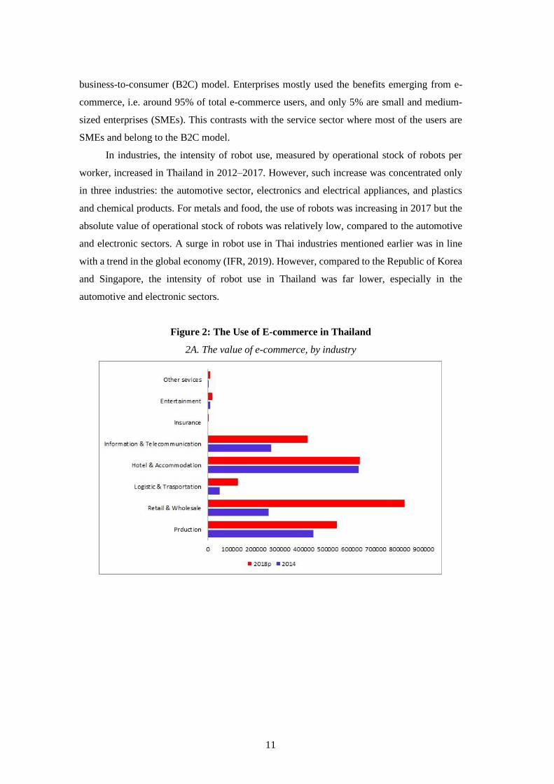
The use of e-commerce in the manufacturing sector expanded in 2014–2017, but its

value was far lower than that in the service sector, especially retail and wholesale and hotel

and accommodation (Figure 2A). In the manufacturing sector, paper, wood and furniture,

plastics, and apparel and textile tended to increasingly use e-commerce over the period 2014–

2017. By contrast, due to the nature of the industry where direct buying is still crucial, the use

of e-commerce in automotive, electronics, and electrical appliances and machines were

relatively low and stable. E-commerce utilised in the manufacturing sector is mostly around

91% in the form of a business-to-business (B2B) model whilst another 9% is in the form of

11

business-to-consumer (B2C) model. Enterprises mostly used the benefits emerging from e-

commerce, i.e. around 95% of total e-commerce users, and only 5% are small and medium-

sized enterprises (SMEs). This contrasts with the service sector where most of the users are

SMEs and belong to the B2C model.

In industries, the intensity of robot use, measured by operational stock of robots per

worker, increased in Thailand in 2012–2017. However, such increase was concentrated only

in three industries: the automotive sector, electronics and electrical appliances, and plastics

and chemical products. For metals and food, the use of robots was increasing in 2017 but the

absolute value of operational stock of robots was relatively low, compared to the automotive

and electronic sectors. A surge in robot use in Thai industries mentioned earlier was in line

with a trend in the global economy (IFR, 2019). However, compared to the Republic of Korea

and Singapore, the intensity of robot use in Thailand was far lower, especially in the

automotive and electronic sectors.

Figure 2: The Use of E-commerce in Thailand

2A. The value of e-commerce, by industry

12

2B. The use of e-commerce adjusted, by gross output

Source: Electronic Transactions Development Agency (ETDA) (2014 and 2018) and Office of the National

Economic and Social Development Council (2014 and 2017).

Figure 3: Intensity of Robot Use in Thailand

3A. Intensity of robot use in Thailand

13

3B. Intensity of robot use in Thailand and other Asian countries in 2017

Note: Figure 3A shows the intensity of robot use in Thailand, measured by operational stock of robots per worker

whilst Figure 3b presents the intensity of robot use in Thailand and other Asian countries in 2017.

Source: International Federation of Robotics (IFR) and National Statistical Office (NSO) (2012 and 2017).

When employment and wage in Thailand are considered, Figure 4 shows that the share of

employment to total employment in the manufacturing sector was relatively stable at around

17% in 2014–2019 whilst that in the service sector had increased to around 52% since 2014,

from around 47% in 2011. For the agriculture sector, the share of employment declined

significantly from 40% in 2013 to around 32% in 2019. The labour force survey, in which

50% of samples at time t-1 are matched exactly with those at time t so that we can construct a

2-year panel data, shows that most workers moving to the service sector are from the

agriculture sector.4 Average wage, measured by baht per month, in the manufacturing and

service sectors increased sharply in 2011–2014 and improved gradually in 2015–2019. Wage

in agriculture by contrast had showed a relatively low and stable rate since 2011. The service

and manufacturing sectors had a wage rate higher than the agriculture sector by around two

times. Agriculture is the only sector in which wage rate in some years, e.g. in 2015 and 2018,

was adjusted lower than headline inflation.

4 Note that, in this study, we consider only workers in the manufacturing sector due to limited data in technological

advancement.

14

Figure 4: Employment and Wage in Thailand, by Industry

4A. Share of employment by sector

4B. Wage (baht per month) by sector

Source: National Statistical Office (2011-2019).

In the manufacturing sector, more than 30% of workers are in food and beverage,

followed by clothing and textile, electronics, and plastics and chemicals. Comparing between

2012 and 2017, employment increased noticeably in the food sector whilst it showed a

declining trend in some sectors, including clothing and textile, automotive, and electronics.

For the other sectors, employment during these two periods was relatively stable. The picture

of wage is different. Sectors, which have a relatively lower share of labour, such as in

automotive, plastics and chemicals, and paper and electronics, tended to offer higher wages.

In the clothing and textile and food sectors, workers receive lower wage (as well as net

income)5 whilst workers in automotive, plastic and chemicals, and paper receive the highest

wage rate. Due to different patterns of wage and employment, this study examines the

reallocation of workers along with wage changes.

5 Note that net income refers to wage and other benefits for workers, including overtime payments and bonus.

15

Figure 5: Employment and Wage in Thai Manufacturing Sector

5A. Share of employment by sector

5B. Wage (baht per month) by sector

Source: Labour force survey, National Statistical Office (2012 and 2017)

16

4. Empirical Model and Data Sources

4.1 Empirical Model

Empirical models applied in this study are based on a framework developed by

Acemoglu and Restrepo (2018b) where the central unit of production is a task, and labour and

capital have comparative advantages in different tasks. An example of a task-based approach

is textile production. It requires many tasks, including production of fibre, production of yarn,

production of fabric, pre-treatment, dyeing and printing, as well as design, marketing, and

retail (see Acemoglu and Restrepo, 2018b). In each task, labour has different comparative

advantages. For example, (skilled) labour tends to have more comparative advantages than

capital in design and marketing. With a task-based framework, automation could substitute

labour in task and reduce demand for labour and wages, the so-called displacement effect. This

is different from applying factor-augmenting technology framework where, in general, labour

demand is expanded along with productivity improvement, except in a case where elasticity

of substitution between capital and labour is small. However, as Acemoglu and Restrepo

(2018b) argued, the demand for labour may eventually not be reduced from the displacement

effect when productivity improvement in a subset of tasks induces more demand for labour in

non-automated tasks, if technology advancements increase capital intensity of production, and

if the deepening of automation leads to intensifying the productive use of machines and

stimulating more demand for labour.

To examine the impacts of technological advancement on job displacement and possible

skill reallocation in the manufacturing sector, an equation examining the probability of being

employed, unemployed, or changing jobs/skills induced by technological advancement is

used. Technological advancements could change employment status – from being employed

to unemployed (and vice versa), from being employed in one task/job to another job – or

maintain the status quo. On changing tasks/jobs, workers can change skills in both directions,

i.e. from skilled to unskilled and vice versa. Whilst there is no guarantee that changing

jobs/tasks results in higher wage/income, this study brings examines the impacts of

technological advancements on wage and income along with skill changes. Eight possible

scenarios could occur from technological advancement when both employment status and

wage/income are considered together, as follows: (1) workers who are employed at the same

task/job and wage/income becomes higher; (2) workers employed at the same task/job, but

wage/income is lower (or unchanged); (3) workers changing skills, from unskilled to skilled

task/job, and wage/income is higher; (4) workers changing skills, from unskilled to skilled

task/job, but wage/income becomes lower (or unchanged); (5) workers changing skills, from

17

skilled to unskilled, but wage/income is higher; (6) workers changing skills, from skilled to

unskilled, and wage/income is lower (unchanged); (7) workers who lose jobs; and (8) workers

who move from unemployed to employed. The eight possible scenarios are constructed from

the Thai Labour Force Survey (National Statistical Office (NSO), 2012–2017), which is

described in detail in section 4.2.

Note that technological advancements in this study are proxied by three key aspects

according to their involvement in the manufacturing supply chains – (i) inbound (automated

e-sourcing), (ii) outbound (e-commerce), and (iii) internal production (e.g. factory automation)

(UNCTAD, 2017) – to delineate the relative important effects of technology involvements in

supply chains in the labour market. As mentioned in the analytical framework, trade is another

important variable, which can shape labour markets. Import penetration, both in terms of

finished, capital, and raw materials, is included in our analysis to compare its effects on

possible skill and wage adjustments. Equation (1) shows variables included in examining the

probability of being employed, unemployed, or changing jobs/skills as follows.

1 1 1, , 0 1 , 1 2 , 1 3 , , 1 , , , ,t t t ti j t j t j t i j t i j t i j tEmployS Technology IMpen IControl − − −− − −= + + + + +

(1)

where , ,ti j tEmployS is the employment status of individual i, sector j at time t. To derive

, ,ti j tEmployS at time t, employment status of individual i is compared between two periods

and see whether at time t workers change skills/tasks from period t-1. To determine workers’

skills/tasks, job position and wage/total income provided in the labour force survey are applied

(see section 4.2). As mentioned, there are eight possible scenarios so that we can identify

change of employment status for individual workers as follows:

, ,ti j tEmployS = 1 for workers who are employed at the same task/job, and wage/income

becomes higher

, ,ti j tEmployS = 2 for workers employed at the same task/job, but wage/income is lower (or

unchanged)

, ,ti j tEmployS = 3 for workers changing skills, from unskilled to skilled task/job, and

wage/income is higher

, ,ti j tEmployS = 4 for workers changing skills, from unskilled to skilled task/job, but

wage/income becomes lower (or unchanged)

18

, ,ti j tEmployS = 5 for workers changing skills, from skilled to unskilled, but wage/income is

higher

, ,ti j tEmployS = 6 for workers changing skills, from skilled to unskilled, and wage/income is

lower (unchanged)

, ,ti j tEmployS = 7 for workers who lose jobs, and

, ,ti j tEmployS = 8 for workers who move from unemployed to employed.

1 , 1tj tTechnology− −

represents technological advancement in industry j at time t-1.

Since changing job position between time t-1 and t would be influenced by

technological advancement at time t-1, we employ lag values of three proxies to represent

technological advancement along the manufacturing supply chains. The three proxies are

composed of

(1) 1 , 1tj tICTUSE− −

= ICT uses per worker in sector jt-1 at time t-1

(2) 1 , 1tj tecommerce− −

= value of e-commerce as percent of GDP in sector jt-1 at time t-1

(3) 1 , 1tj trobot− −

= intensity of industrial robot uses (operational stock of robots per worker)

in sector j at time t-1

Note that once workers move to new tasks at time t, the new tasks might not be in the

same industry as those at time t-1. In other words, industry j and industry jt-1 could be different.

The endogeneity problem is redressed from employing lag values of technological

advancement.

1 , 1tj tIMpen− −

is import penetration in industry jt-1 at time t-1. Import penetration is measured by

the share of import at industry j to GDP.6 Import penetration is further divided into finished

products (1 , 1_

tj tIMpen finish− −

), capital (1 , 1_

tj tIMpen cap− −

) and raw materials

(1 , 1_

tj tIMpen raw− −

).

1 , 1tj tIControl− −

is control variables for individual workers i in industry jt-1 at time t. This

includes age, gender, and education.

6 The results are robust, though we measure import penetration as the share of import at industry jt-1 to total

supply (GDP and imports).

19

, ,i j t is an unobserved industry-specific effect and , ,i j t is the error term.

The impacts of advanced technology and import penetration are examined sector-wise. Five

key sectors in Thailand are examined: (i) food and beverage, (ii) clothing and textile, (iii)

plastics and chemicals, (iv) electronics and machinery, and (v) automotive. To investigate such

impacts, interaction terms between proxies of technology/import penetration and industry-

dummy variables are introduced in the model as in equation (2).

( )

( )1 1 1 1

1 1 1

, , 0 1 , 1 2 , 1 3 , 1 , 1

4 , 1 , 1 5 , , 1 , , , ,

t t t t t

t t t

i j t j t j t j t j t

j t j t i j t i j t i j t

EmployS Technology IMpen Technology DumINDUS

Mpen DumINDUS IControl

− − − −

− − −

− − − −

− − −

= + + +

+ + + +

(2)

where 1 , 1tj tDumINDUS− −

is industry-dummy variables, composed of five key sectors, as

mentioned earlier: (i) food and beverage (dumfood), (ii) clothing and textile (dumcloth), (iii)

plastics and chemicals (dumplas), (iv) electronics and machinery (dumelec), and (v)

automotive (dumauto).

As discussed in section 4.2, due to the process of data collection in the labour force

survey, around half of observations from the survey are used to identify , ,ti j tEmployS . To

ensure the impact of technological advancement on labour outcome, especially on wage/total

income, another equation is introduced to examine the impacts of technological advancement

on individual wage/income by using the whole observations in the manufacturing sector.7

Equation (3) is a wage/income equation, which could be affected by technological

advancement and import penetration.

, , ,, , 0 1 2 , 3 , ,i j ti j t j t j t j t jtw M IConty rolage Technolog I pen = + + + + + (3)

where , ,i j twage is wage (measured by baht per month) of worker i in sector j at time t. Since

we control for year fixed effect, nominal instead of real wage (nominal wage adjusted by

consumer prices) is employed. In this study, we employ both wage and total income, which is

7 We also analysed the impacts of technological advancement on employment also by specifying a dummy variable

equal to 1 if workers are employed, and 0, if not. The results are similar to those in equation (1) when half of the

observations are used. We did not examine the effects of employment at the industry level due to limited data,

especially when we tried to control for industry-specific effects (by including industrial dummy variables) and

using two-stage least squares to redress the endogeneity problem.

20

wage plus overtime payments and bonus. As discussed in section 4.2, we also use lag values

of technology and import penetration to examine such impacts on wage. The results are like

those when current value (time t) of technology and import penetration are employed.

4.2 Data and Methodology

The Thai Labour Force Survey of the NSO, in 2012–2017, was used to construct

employment status (, ,ti j tEmployS ). Although the NSO conducts a labour force survey every

quarter, we conduct our analysis annually due to data collection of our technology variables.8

To avoid overestimation of employment, which arises from temporary workers, in either the

manufacturing or the service sectors, we use information from the third quarter of the labour

force survey, i.e. during a harvest season. The process of data collection in the labour force

survey allows us to examine the status of workers between period t and period t-1. Table 1

shows how observations were included in the Thai Labour Force Survey.

Table 1: Observations Included in the Thai Labour Force Survey

Sampling

Sampling

(40%–

50%)

2012 Q3 1C 2C

2013 Q3

2C 3C

2014 Q3

3C 4C

2015 Q3

4C 5C

2016 Q3

5C 6C

2017 Q3 6C 7C

Source: Authors, adopted from the Thai Labour Force Survey.

From Table 1, the NSO divided samples in the labour force survey into two groups: 1C

and 2C in 2012Q3 and 2C and 3C in 2013Q3. For every year, around 50% of samples in the

labour force survey at time t-1 were matched precisely with those at time t. In 2012Q3, a group

of persons in 2C were the same persons in 2013Q3, and a group of persons in 3C in 2013Q3

were the persons in 2014Q3. Thus, from the survey, we can have a 2-year panel, which can be

used to determine whether a worker changes jobs from skilled to unskilled or vice versa, or

becomes employed to unemployed or vice versa, or maintains the status quo. Along with

8 Note that a sampling method of each quarter is similar to that on an annual basis, i.e. only half of observations

in the current quarter (e.g. second quarter) are matched with the previous quarter (first quarter).

21

changing employment status, we looked at how wage/income is adjusted over the 2-year panel.

Note that in the construction of employment status and wage/income changes, we excluded

workers who are not in the labour force, such as persons who are studying, disabled, older than

75 years, and those who do not specify their wage and other incomes. Due to limited data on

technology variables, our analysis focused only on the manufacturing sector, as classified by

the Thailand Standard of Industrial Classification, (TSIC 10-32), excluding the agriculture and

the service sectors.

To determine workers’ changing position from skilled to unskilled, or vice versa, we

used job position as provided in the labour force survey. Eight principal positions in each

industry were classified in the survey: (1) executive manager, (2) manager, (3) professional,

(4) associate professional, (5) technicians, (6) services and sale workers, (7) clerical support

work, (8) basic job (Table 2). A worker who moves up a position, e.g. from services and sale

worker to technician or to associate professional, is classified as changing from an unskilled

to skilled job. By contrast, a worker changing jobs, say, from associate professional to

technician or to services and sale worker is classified as changing from a skilled to an unskilled

job. As mentioned in the previous section, we used only job position and wage/total income

as criteria to construct , ,ti j tEmployS . Thus, a worker classified as relatively unskilled in one

industry can become more skilled within the same industry or in another industry. Workers

who are employed but do not change position status are classified as employed workers and

status quo, i.e. , ,ti j tEmployS = 1 or 2 depending on wage/income of those workers. By

contrast, if employed workers at time t-1 become unemployed at time t, they are classified as

, ,ti j tEmployS = 7; vice versa, they are classified as , ,ti j tEmployS = 8.

Table 2: Occupation Codes Used to Define Employment Status

Changing

Skills

Occupation

Code

Skilled to

Unskilled

Unskilled to

Skilled

1 Executive manager 1111-1120

2 Manager 1211-1439

3 Professional 2111-2659

4 Associate

professional

3111-3522

5 Technician 6111-8350

6 Service and sale

worker

5111-5419

7 Clerical support

work

4110-4419

8 Basic job 9111-9629

Source: Thai Labour Force Survey (2012–2017).

22

Table 3 shows the frequency of employment status and distribution of workers amongst

eight categories (EmploySi,j,t) during 2012–2017. It seems that EmploySi,j,t = 2 has the highest

frequency, followed by EmploySi,j,t = 1. This shows that in the manufacturing sector, most

workers in the survey were employed at the same occupation position and income level during

the 2-year panel, on average around 50% of total observations. This is not surprising as our

panel is short. In fact, it would be better if we could construct EmploySi,j,t from a long period

of panel data as normally changing occupation positions takes time. However, the technology

involved in moving the country towards Industry 4.0, such as robots/automation, could create

a possible disruption on labour market outcome. Thus, analysing the impacts of such

technological advancements through a short-panel data would probably yield some interesting

findings. In addition, the survey revealed changes in workers’ occupation positions during the

2-year panel. For example, in almost 10% of observations, workers moved from unskilled to

skilled positions, with around 5% of workers receiving higher incomes. In almost another 10%

of observations, workers changed positions from skilled to unskilled, with around 6% of

workers receiving lower payments.

For technology variables, ICT use in industries was from the ICT survey of the NSO.

Employment in industries was used to adjust the ICT data to be in terms of ICT use per worker.

Data on e-commerce use in industries were from the value of e-commerce survey, Electronic

Transactions Development Agency. Gross output at the industry level, from the Office of the

National Economic and Social Development Council, was employed to adjusted e-commerce

data. Data on operational stock of robots were from the International Federation of Robotics,

and employment at the industry level was applied to adjust robotic data in terms of intensity

of robot use. Import data were from UNCOMTRADE, United Nations Commodity Trade

Statistics Database. We used import data at the 4-digit Harmonized System code and

converted them into 2-digit International Standard Industry Classification using product

concordance from the United Nations. Import data were adjusted by gross output at the 2-digit

industry level. Note that import data were divided into finished, capital, and raw material

products using Broad Economic Categories rev. 4. Age, gender, and education from the labour

force survey were used as control variables in equations (1) to (3).

23

Table 3: Frequency of Employment Status and Income Changes (, ,ti j tEmployS ) amongst Eight Categories in 2012–2017

Total 2013 and 2012 2014 and 2013

Employment/income status Freq. Percent Cum. Freq. Percent Cum. Freq. Percent Cum.

1 5.880 27,11 27,11 1 1.154 28,97 28,97 1 1.119 26,74 26,74

2 11.569 53,34 80,45 2 1.772 44,49 73,46 2 2.133 50,98 77,72

3 1.130 5,21 85,66 3 325 8,16 81,62 3 218 5,21 82,93

4 977 4,5 90,17 4 272 6,83 88,45 4 201 4,8 87,74

5 735 3,39 93,56 5 164 4,12 92,57 5 177 4,23 91,97

6 1.277 5,89 99,45 6 272 6,83 99,4 6 316 7,55 99,52

7 69 0,32 99,76 7 13 0,33 99,72 7 11 0,26 99,78

8 51 0,24 100 8 11 0,28 100 8 9 0,22 100

Total 21.688 100 Total 3.983 100 Total 4.184 100

2015 and 2014 2016 and 2015 2017 and 2016

Employment/income status Freq. Percent Cum. Freq. Percent Cum. Freq. Percent Cum.

1 1.170 26,22 26,22 1 1.171 26,19 26,19 1 1.266 27,6 27,6

2 2.578 57,76 83,98 2 2.512 56,18 82,38 2 2.574 56,12 83,71

3 203 4,55 88,53 3 189 4,23 86,6 3 195 4,25 87,97

4 153 3,43 91,96 4 182 4,07 90,67 4 169 3,68 91,65

5 124 2,78 94,73 5 127 2,84 93,51 5 143 3,12 94,77

6 210 4,71 99,44 6 263 5,88 99,4 6 216 4,71 99,48

7 20 0,45 99,89 7 15 0,34 99,73 7 10 0,22 99,69

8 5 0,11 100 8 12 0,27 100 8 14 0,31 100

Total 4.463 100 Total 4.471 100 Total 4.587 100

Note: We used total income, including salary, overtime payment, and bonus, to define employment status and income changes. The result is robust when wage is used instead of total

income as salary is a key component in total income.

Source: Authors’ calculation.

24

The data for analysing impacts of technological advancements and import penetration

on change in employment status as well as income changes are summarised in Table 4. Per

section 4.1, due to the data collection process in the labour force survey, around half of

observations from the survey are thrown away when impacts of technological advancement

on employment status and income change (EmploySi,j,t) are analysed. To ensure the impacts

of technological advancement on labour outcome, especially wage/total income, another

equation (equation 2) is employed to examine the impacts of technological advancement on

individual income by using the whole observations in the manufacturing sector. Data for

analysing individual income are shown in Table 5.

Table 4: Data Summary, 2012–2017

Variable Obs. Mean Std. Dev. Min. Max.

EmploySi,j,t 21,688 2.24 1.36 1 8

agei, jt-1,t-1 21,688 39.39 11.92 14 74

sexi,j,t 21,688 1.53 0.50 1 2

educationi, jt-1,t-1 21,688 0.74 0.75 0 3

ICTUSEi, jt-1, t-1 21,688 0.13 0.22 0.04 2.27

ecommercei, jt-1, t-1 12,777 0.03 0.12 0 2.12

roboti, jt-1, t-1 19,665 2.22 4.58 0 22.91

IMpeni, jt-1, t-1 16,275 1.73 2.81 0 180.85

IMpen_finishi, jt-1, t-1 16,257 25.24 53.95 0 829.98

IMpen_capitali, jt-1, t-1 16,257 3.13 14.08 0 366.13

IMpen_rawi, jt-1, t-1 16,257 2.05 14.36 0 502.23

wagei, jt-1, t-1 21,688 8150.85 9888.00 0 400000

totalincomei, jt-1, t-1 21,688 9110.38 10677.96 0 400000

Notes: Data for e-commerce are from 2014 to 2017 while for other variables, data start from 2012 to 2017. Sex,

which is equal to ‘1’, represents male whilst ‘2’ represents female. Education comprises four ranks, i.e. ‘0’

represents lower or equal to primary education; ‘1’ represents lower secondary education; ‘2’, upper secondary and

post-secondary education; ‘3’, bachelor’s degree and higher.

Source: Authors’ calculation.

25

Table 5: Data Summary for Wage/Income Analysis, 2012–2017

Variable Obs. Mean Std. Dev. Min. Max.

roboti, j, t 88,059 1.66 4.39 0 25.93

roboti, jt-1, t-1 72,936 2.10 4.43 0 22.91

ICTUSEi, j, t 96,654 0.14 0.22 0.04 2.27

ICTUSEi, jt-1, t-1 79,863 0.14 0.24 0.04 2.27

ecommercei, j, t 59,891 0.03 0.12 0 2.12

ecommercei, jt-1, t-1 44,556 0.03 0.14 0 2.12

IMpeni, j, t 72,959 1.82 3.02 0 226.76

IMpen_rawi, j, t 72,872 29.69 60.02 0 1038.03

IMpen_capitali, j, t 72,872 3.01 13.76 0 366.13

IMpen_finishi, j, t 72,872 2.09 14.07 0 502.23

IMpeni, jt-1, t-1 60,745 1.82 3.06 0 226.76

IMpen_rawi, jt-1, t-1 60,668 28.85 56.86 0 829.98

IMpen_capitali, jt-1, t-1 60,668 2.92 14.17 0 366.13

IMpen_finishi, jt-1, t-1 60,668 2.02 12.89 0 502.23

agei, j,t 96,654 39.40 12.57 15 75

sexi,j,t 96,654 1.53 0.50 1 2

educationi, j,t 96,654 0.27 0.64 0 3

wagei, j, t 68,426 10790.30 9338.26 0 400000

totalincomei, j, t 68,426 12951.52 16101.70 0 450000

Source: Authors’ calculation.

The multinomial (polytomous) logistic and probit regression models are employed to

analyse the impacts of technological advancement on employment status and income changes

(equation 1). The multinomial logit model is chosen since outcomes of the model have no

natural ordering. The multinomial probit is employed as an alternative model to check the

robustness of our results. Results are interpreted in terms of elasticity using margin estimates

for both multinomial logistic and probit models. Since the lag values of all independent

variables are used in the model, the endogeneity problem is less of a concern in the model.

However, to redress a possible self-selection problem in which technology may self-select into

industries where workers have a high tendency to move up the ladder, a control function

approach in which an endogenous predictor is instrumented in a first step using ordinary least

squares (OLS) and then including the residuals in the second step in multinomial response

model (Petrin and Train, 2010).9

9 Regarding an instrument, we use a lag of its variable as an instrument for technology variable. In fact, it may be

better to use other variables such as progress in technologies in other Asian countries as an instrument variable.

26

For the individual income/wage equation, two-stage least squares is employed to redress a

problem of endogeneity, and lag values of independent variables are used as instruments.

5. Results

Table Appendix 1 presents the results of equation (1) by using multinomial logistic

regression model where a possible endogeneity problem is redressed by using a control

function approach.10 Tables 6 and 7 show the results of equations (1) and (2), respectively, in

terms of elasticity by using margin estimates. For Table 6, columns A–C, proxies of

technology variables – namely, ICT, robot, and e-commerce – are estimated separately whilst

in column D, these three proxies of technology are estimated together. The results of both

methods are similar. However, based on indicators of explanatory power, such as LR-chi 2

and log likelihood, our analysis below is based on the former method where proxies of

technology variables are separately estimated.

When the whole manufacturing sector is concerned, there is no evidence that

advancement in technology had so far pushed workers out of the job market in Thailand.

Coefficients associated with three proxies of technology – ICT use, robots, and e-commerce –

in outcome no. 7 (EmploySi,j,t = 7) are all statistically insignificant (Table 6, columns A–C).11

This implies that statistically no worker becomes unemployed when more advanced

technology is introduced in supply chains. However, when each sector is investigated

separately, advancement in ICT use seems to increase the probability of workers in the food

and beverage sector moving from employed to unemployed. The elasticity associated with

ICTUSE in the food and beverage sector for outcome no. 7 (EmploySi,j,t = 7) is positive and

statistically significant. This implies that an increase in ICT use per worker by 1% raises the

probability of workers becoming unemployed by 0.1% (Table 7, column A). The distribution

of occupations in the food and beverage sector could explain such finding. Table 8 shows a

high proportion of workers who were in a ‘basic job’ category, such as drivers who deliver

products, sellers of products in a small shop, and cleaners, in the food and beverage sector.

However, with limited data, especially the value of e-commerce at the industry level, a lag of its technology

variable is used instead. 10 Note that independence of irrelevant alternatives (IIA), where the choice between a collection of alternatives is

not affected by non-chosen alternatives, is tested in all regressions based on the Hausman and McFadden (1984)

test. In all outcomes (outcomes 1–8), we accept the null hypothesis where the IIA assumption is satisfied. In some

cases, the chi-2 turns out to be negative. However, as mentioned in Hausman and McFadden (1984, p.1226), a

negative result is evidence that the IIA has not been violated. In addition, the multinomial probit regression model

yields similar results to the multinomial logit model so that we analyse our findings through a multinomial logistic

model. 11 When all three proxies of technology are included together in equation (1), the results are similar to those when

all proxies are included in the equation separately.

27

Workers in this category can be easily replaced by technology. In other sectors, a proportion

of workers who were in a ‘basic job’ were far lower. For example, in the electronics and the

automotive sectors, a proportion of workers who were in a basic job was only 4.5% and 6.1%

of the total workforce, respectively. Interestingly, the results show that only ICT use, not

robots or e-commerce, could push workers out of the job market. A relatively lower

penetration of robots and e-commerce than ICT use may limit the impacts of these

technologies on job destruction in Thailand. In other words, to some certain extent, the

displacement effect induced by advanced technologies mentioned in Acemoglu and Restrepo

(2018a, 2018b, 2019) is still limited in Thai manufacturing.

Although the impact of advanced technology in pushing workers out of the job market

in Thailand is limited, it tends to affect the reallocation of workers between skilled and

unskilled positions.12 This finding is similar to Dauth et al. (2018) who used Germany as a

case study and showed that the displacement effect was minimal as workers tended to either

stay with their original employer or switch occupations at their original workplace. Evidence

from the Thai Labour Force Survey showed that around 70% of total workers who stayed at

the same positions (outcomes no. 1 and 2) remained in the same industries. However, in

contrast to Dauth et al. (2018), our evidence reveals that only 50% of total workers who

changed their positions (outcomes no. 3 to 6) switched within the same industries (Figure 6A).

For another 50%, changes in positions occurred across industries, and such reallocation was

shown obviously in five industries: (i) food and beverage, (ii) electronics, (iii) plastics and

chemicals, (iv) textiles, and (v) automotive (Figure 6B). In the food and beverage sector,

however, the survey showed that reallocation of workers within the industry was almost two

times higher than across industries (Figure 6C). This may imply either a relatively high

demand for workers in this sector or less flexibility of workers in adjusting to shocks,

especially when a high proportion of workers in this sector were willing to switch positions

from a skilled to an unskilled position (Figure 6C).

12 Note that due to the model setting, evidence of the reallocation of workers would not well provide evidence of

the reinstatement effect where new tasks would be created from introducing new technology as shown in Acemoglu

and Restrepo (2019). Jobs, which workers reallocate, could be either new or existing tasks in industries.

28

Figure 6: Proportion of Workers Who Switch Job Positions

Figure 6a: Proportion of workers who switch positions across industries

(% of total workers who switch position)

Figure 6b: Reallocation of workers across industries by sector

(% of total workers who switch positions)

29

Figure 6c: Reallocation of workers within industries by sector

(% of total workers who switch positions)

Source: Authors’ compilation from the Thai Labour Force Survey.

The results vary amongst proxies of technology and sectors. For ICT use in the entire

manufacturing sector, the technology tends to lower the probability of shifting workers from

unskilled to skilled positions. This is shown by a negative and statistical significance of

coefficients associated with ICTUSE for outcome no. 4 (EmploySi,j,t = 4) (Table 6, column

A). The negative sign reflects that a 1% increase in ICT use per worker results in a lower

probability (0.07%) of workers moving from unskilled to skilled jobs. Sector-wise, such

negative impacts are found in relatively high capital-intensive industries, including

automotive, plastics and chemicals, and electronics and machinery. Coefficients associated

with the interaction term between ICTUSE and industrial dummy variables in these sectors for

outcome no. 4 (EmploySi,j,t = 4) are statistically insignificant (Table 7, column A).

30

Table 6: Impacts of Advanced Technology on Employment Status and Income Changes (Elasticity Estimation)

Column A Column B Column C Column D

ICTUSEi, jt-1, t-1 roboti, jt-1, t-1 ecommercei, jt-1, t-1 ICTUSEi, jt-1, t-1 roboti, jt-1, t-1 ecommercei, jt-1, t-1

_predict Coefficient Z Coefficient Z Coefficient Z _predict Coefficient Z Coefficient Z Coefficient Z

1 0,002 0,18 0,013 1,11 0,001 0,14 1 -0,012 -0,79 -0,005 -0,27 -0,005 -0,79

2 0,005 0,94 -0,012 -1,17 0,000 -0,01 2 0,015 2,38 0,012 0,83 0,004 1.65*

3 0,024 1,07 -0,026 -0,78 -0,019 -1,04 3 -0,022 -0,66 -0,037 -0,65 -0,031 -1,38

4 -0,073 -2.13** 0,009 0,23 0,016 1.68*** 4 -0,085 -1.91** -0,006 -0,09 0,011 1,08

5 0,026 0,8 0,031 0,76 -0,020 -0,85 5 0,023 0,48 0,014 0,21 -0,029 -0,92

6 -0,029 -1,11 -0,023 -0,71 0,007 0,67 6 -0,039 -1,15 -0,026 -0,48 0,000 -0,02

7 -0,074 -0,6 0,025 0,20 -0,115 -0,88 7 -0,196 -1,05 -0,142 -0,83 -0,101 -0,75

8 -0,180 -0,98 0,064 0,59 -0,066 -0,8 8 -0,161 -0,65 -0,092 -0,39 -0,060 -0,63

IMpeni, jt-1, t-1 IMpeni, jt-1, t-1 IMpeni, jt-1, t-1 IMpeni, jt-1, t-1

_predict Coefficient Z Coefficient Z Coefficient Z _predict Coefficient Z

1 -0,036 -3.33*** -0,040

-

3.35*** -0,054

-

3.27*** 1 -0,063

-

3.61***

2 0,012 2.01** 0,014 2.13** 0,016 1.98** 2 0,019 2.27**

3 -0,030 -1,06 -0,035 -1,14 -0,024 -0,55 3 -0,029 -0,64

4 0,085 3.92*** 0,089 3.93*** 0,124 3.26*** 4 0,127 3.26***

5 -0,086 -2.27** -0,101 -2.45** -0,082 -1,53 5 -0,095 -1.69*

6 0,051 2.37** 0,058 2.56*** 0,043 1,19 6 0,050 1,35

7 -0,184 -1,21 -0,189 -1,16 -0,156 -0,75 7 -0,100 -0,48

8 -0,208 -1,33 -0,267 -1,52 0,050 0,29 8 0,083 0,46

Industry

dummy Yes Yes Yes Industry dummy Yes

Year

dummy Yes Yes Yes Year dummy Yes

Number

of obs 16.275 14.169 9.344 Number of obs 8.820

LR chi2 2371,90 2043,47 963,35 LR chi2 950,56

Prob >

chi2 0,00 0,00 0,00 Prob > chi2 0,00

Pseudo

R2 0,0553 0,0534 0,0408 Pseudo R2 0,0425

Log

likelihood -20255.424 -18107.519 -11310,391 Log likelihood -10708,156 Notes: Numbers 1 to 8 correspond to a change in employment status and income changes as identified in equation (1). ***, **, and * represent 1%, 5%, and 10% significant level, respectively. In columns A to C, proxies of technology variables – namely, ICT, robot, and e-commerce – are estimated separately whilst in column D, these three proxies of technology are estimated together. Elasticities estimated in this table are from results reported in Appendix I. Source: Authors’ estimation.

31

The impacts of ICT use on employment status tend to be more noticeable in the

automotive sector than in the other two sectors (plastics and chemicals, and electronics and

machinery). In the automotive sector, the probability of workers moving from skilled to

unskilled jobs increases when ICT is used more. This evidence occurs in a group of workers

whose income does not adjust according to skill changes reflected by a positive and

statistically significant coefficient associated with the interaction term between ICTUSE and

industrial dummy variables of the automotive sector for outcome no. 6 (EmploySi,j,t = 6). By

contrast, in the electronics and machinery sector, introducing more ICT benefits some groups

of workers in the sector. This is reflected by the higher probability that workers could move

from unskilled to skilled positions and receive higher income payments, i.e. the coefficient

associated with the interaction term between ICTUSE and industrial dummy variables of

electronics and machinery for outcome no. 3 (EmploySi,j,t = 3) is positive and statistically

significant (Table 7, column A). Meanwhile, introducing ICT helps some groups of workers

in this sector to stay in skilled positions, as the coefficient associated with the interaction term

between ICTUSE and industrial dummy variables of electronics and machinery for outcome

no. 5 (EmploySi,j,t = 5) is negative and statistically significant (Table 7, column A). This

implies that an increase in ICT use by 1% results in a 0.13% decline in the probability of

workers moving from skilled to unskilled positions.

Table 7: Impacts of Advanced Technology on Employment Status and Income

Changes, by Sector (Elasticity Estimation)

_predict

Column A Column B Column C

ICTUSEi, jt-1, t-1 roboti, jt-1, t-1 ecommercei, jt-1, t-1

Coefficient Z Coefficient Z Coefficient Z

1 -0,001 -0,07 -5,660 -1.86** -0,001 -0,13

2 0,007 1,24 5,316 2.23** 0,001 0,62

3 0,015 0,62 -11,360 -1,53 -0,013 -0,72

4 -0,089 -2,2 10,200 1,09 0,015 1.66*

5 0,056 1.69* -30,237 -2.78*** -0,027 -0,96

6 -0,027 -0,97 17,140 2.00** -0,003 -0,27

7 -0,135 -0,74 -21,088 -0,59 -0,238 -0,92

8 -0,256 -1,03 22,001 0,34 0,001 0,02

ICTUSEi, jt-1, t-

1*dumfood roboti, jt-1, t-1*dumfood

ecommercei, jt-1, t-

1*dumfood

_predict

1 0,016 1.68* 1,603 2.10** -0,038 -0,02

2 -0,009 -1.89* -0,613 -1.94** -0,013 -0,01

3 0,025 1,35 2,728 1.78* -0,051 -0,03

4 0,030 1.62* -1,595 -0,84 0,009 0,01

32

5 -0,012 -0,44 6,568 2.97*** -0,065 -0,04

6 -0,017 -0,73 -3,005 -1.73* -0,079 -0,04

7 0,111 2.04** 4,262 0,59 12,7 0,01

8 0,123 1,17 -4,256 -0,33 0,092 0,05

ICTUSEi, jt-1, t-

1*dumcloth

ecommercei, jt-1, t-

1*dumcloth

_predict

1 -0,017 -2.07** 0,004 2.26**

2 0,011 2.60*** -0,002 -1,5

3 -0,018 -0,65 -0,004 -0,51

4 0,043 1.91** -0,006 -0,63

5 -0,106 -2.06** 0,001 0,06

6 -0,052 -1,52 -0,004 -0,45

7 0,041 0,94 0,021 1,28

8 0,158 1.86* -1,329 -0,01

ICTUSEi, jt-1, t-

1*dumplas roboti, jt-1, t-1*dumplas

ecommercei, jt-1, t-

1*dumplas

_predict

1 0,003 0,46 0,067 1.73* -0,010 -2.58***

2 0,002 0,46 -0,068 -2.28*** 0,001 0,37

3 0,009 0,61 0,164 1.90** 0,001 0,2

4 -0,011 -0,53 -0,115 -1,03 0,006 1,09

5 -0,032 -1,37 0,368 2.84*** 0,007 1,13

6 -0,011 -0,68 -0,189 -1.89** 0,008 2.15**

7 -0,061 -0,35 0,182 0,42 0,036 1,24

8 0,173 1,06 -0,218 -0,28 -1,973 -0,69

ICTUSEi, jt-1, t-

1*dumelec roboti, jt-1, t-1*dumelec

ecommercei, jt-1, t-

1*dumelec

_predict

1 -0,004 -0,28 1,897 1.72* -0,004 -0,77

2 -0,007 -0,48 -2,381 -2.32** 0,011 2.38**

3 0,081 2.17** 4,136 1,44 -0,005 -0,27

4 0,025 0,52 -4,265 -1,16 -0,009 -0,35

5 -0,131 -2.35** 11,555 2.73*** -0,049 -1.81*

6 0,045 1,11 -6,949 -2.07** -0,021 -0,99

7 -0,030 -0,19 8,042 0,58 -0,049 -0,49

8 -0,005 -0,03 -8,428 -0,34 -0,125 -1,21

ICTUSEi, jt-1, t-

1*dumauto roboti, jt-1, t-1*dumauto

ecommercei, jt-1, t-

1*dumauto

_predict

1 0,003 0,71 2,063 1.79* 0,004 1,54

2 -0,006 -1,37 -2,262 -2.19** -0,003 -0,8

3 -0,009 -0,71 4,275 1,46 0,003 0,3

4 0,008 0,59 -4,177 -1,13 -0,009 -0,59

5 -0,005 -0,36 11,703 2.75*** 0,017 2.19**

33

6 0,020 2.12** -6,923 -2.06** -0,029 -1.92**

7 -0,008 -0,18 8,096 0,58 -0,062 -0,71

8 -0,024 -0,41 -8,710 -0,34 -0,045 -0,87

Industry

dummy Yes Yes Yes

Year

dummy Yes Yes Yes

Number

of obs 16.275 14.169 9.344

LR chi2 2426,36 2094 1023

Prob >

chi2 0,00 0,00 0,00

Pseudo

R2 0,0566 0,0547 0,0434

Log

likelihood -20228,191 -18082,257 -11280,568

Notes: ***, **, and * represent 1%, 5%, and 10% significant level, respectively,

There is no information in textile and clothing sector since data on operational stocks of robot use in this sector is

reported as zero during 2002–2016. The small positive number of operational stocks of robot use in clothing and

textile was shown in 2017,

To be consistent with the results in Table 6, proxies of technology variables – namely, ICT, robot, and e-commerce

– are estimated separately in this table.

Elasticities estimated in this table are from results reported in Appendix II.

Source: Authors’ estimation.

Table 8: Proportion of Workers, by Occupation Code and Sector (2012–2017)

Occupation Code

10-12:

Food and

Beverage

13-15:

Textile and

Clothing

19-23:

Plastics and

Chemicals

26-28:

Electronics and

Machinery

29-30:

Automotive

1

Executive

manager 0,10 0,08 0,38 0,16 0,08

2 Manager 3,19 1,62 5,17 3,35 4,42

3 Professional 1,31 0,62 5,07 3,59 3,44

4

Associate

professional 4,14 1,82 8,90 8,87 9,66

5 Technician 61,59 64,52 62,06 74,72 69,53

6

Service and

Sale workers 4,64 0,30 1,50 0,56 0,66

7

Clerical

support work 4,26 28,87 6,60 4,27 6,06

8 Basic job 20,78 2,16 10,31 4,48 6,14

Source: Authors’ calculation from the Thai Labour Force Survey.

In the food and beverage and the clothing and textile sectors, an increase in ICT use

raises the probability of workers to shift their positions from unskilled to skilled as reflected

by a positive and significant coefficient associated with the interaction term between ICTUSE

and industrial dummy variables in these two sectors for outcome no. 4 (EmploySi,j,t = 4)

34

(Table 7, column A). In the food and beverage sector, the use of ICT also helps increase the

probability of workers to stay at the same position and receive higher income payments (the

coefficient associated with ICTUSE for outcome no. 1 is positive and higher than that with

ICTUSE for outcome no. 2).

In the clothing and textile sector, introducing more ICT could maintain workers at the

same job position, but workers who receive such benefit receive relatively lower pay. This is

reflected by a positive and significant coefficient associated with the interaction term between

ICTUSE and industrial dummy variables in this sectors for outcome no. 2 (EmploySi,j,t = 2)

(Table 7, column A). In addition, in this sector, the probability of workers moving from skilled

to unskilled jobs declines when more ICT use is introduced. The coefficient associated with

the interaction term between ICTUSE and industrial dummy variables in this sector for

outcome no. 5 (EmploySi,j,t = 5) is negative and significant.

For the intensity of robot use, its impacts on employment status/income changes emerge

only when the individual sectors are analysed. Workers in the automotive, electronics, and

plastics and chemical sectors tend to get net negative impacts from the introduction of more

robots. First, in these sectors, the probability of workers moving from unskilled to skilled jobs

declines. This is reflected by the positive coefficients associated with the interaction term

between robot and dummy variables in these sectors for outcome no. 3 (EmploySi,j,t = 3).

However, the value is less than the negative value at the base case (Table 7, column B).

Second, the probability of workers staying at the same position and receiving higher payments

declines (EmploySi,j,t = 1) (Table 7, column B). Although the introduction of robots benefits

workers with lower pay – i.e. the probability of workers staying at the same position but whose

income does not adjust (EmploySi,j,t = 2) increases – the magnitude of gains from this group

of workers cannot cover the possible loss that arises from a group of workers whose income

is adjusted upward for staying at the same position. Third, the probability that workers would

change from skilled to unskilled jobs declines (see the net value of coefficients associated with

the interaction term between robot and industrial dummy variables for outcomes no. 5 and 6

(EmploySi,j,t = 5 and EmploySi,j,t = 6) and value of the base case. But when comparing the

net value of elasticity between cases 5 and 6 with that of case 3, the magnitude of case 3 (which

is negative) is higher than cases 5 and 6. This implies that at the net impacts, workers will

likely move from skilled to unskilled jobs. Note that for the third point, less concern is found

for the plastics and chemical sectors (Table 7, column B).

35

For the food and beverage sector, introducing robots helps workers stay at the same

positions but income does not adjust upward, i.e. the coefficient associated with EmploySi,j,t

= 2 is positive and statistically significant. The magnitude of gains from this group of workers

is higher than the possible loss that arises from a group of workers whose income increases

when staying at the same position (EmploySi,j,t = 1) (Table 7, column B). In addition, at the

net impact, there is a lower probability of workers to move from skilled to unskilled jobs. The

net value of elasticity between cases 5 and 6 (in absolute terms) is higher than that of case 3.

All in all, the intensity of robot use has a less severe effect on the food and beverage sector.

Part of the reasons could be the nature of the industry itself, which still needs to rely more on

labour, and the development in technology, which may still not match well with a need in the

food sector. The use of robots in this sector is minimal in Thailand, though increasing,

compared to the above three sectors. The same trend is found globally.

The introduction of e-commerce tends to benefit labour market outcomes. As far as the

whole manufacturing is concerned, the probability of workers shifting to skilled positions from

unskilled ones increases by 0.02% when the value of e-commerce as percent of GDP increases

by 1%. However, a group of workers who moved to better-skilled positions do not receive

higher payments along with skill changes. This is reflected by the positive and significant

coefficient of ecommerce for outcome no. 4, not outcome no. 3 (Table 6, column C). Sector-

wise, the impact of e-commerce on employment status in the food and beverage sector

resembles that of the whole manufacturing sector whilst workers in the clothing and textile as

well as the electronic sectors seem to receive additional benefits from using e-commerce. In

the clothing and textile sector, the use of e-commerce helps workers stay at the same position

and receive higher income (see a positive coefficient associated with the interaction terms

between ecommerce and industrial dummy for outcome no. 1) (Table 7, column C). In the

electronics and machinery sector, e-commerce supports workers to stay at the same position

as in the clothing and textile sector. However, the effect occurs on a group of workers who

receive low payment (see a positive coefficient associated with the interaction terms between

ecommerce and industrial dummy for outcome no. 2). In addition, the probability of workers

moving from skilled to unskilled jobs declines (a negative coefficient associated with the

interaction terms between ecommerce and industrial dummy for outcome no. 5).

The automotive sector receives benefits from using e-commerce, but impacts tend to be

smaller than the above two sectors. The probability of workers moving from skilled to

unskilled jobs goes down for a group of workers who receive lower pay. But this positive

effect is countered by another group of workers who receive higher pay but will likely move

from skilled to unskilled positions (see net elasticity of the interaction terms between

36

ecommerce and industrial dummy for outcomes no. 5 and 6) (Table 7, column C). Evidence

from the labour force survey shows that in the automotive sector, workers who move from

skilled to unskilled positions are mostly from other industries, i.e. reallocation across

industries (Figure 6B).

In contrast to other sectors, e-commerce seems to negatively impact employment status

in the plastics and chemical sector. The probability of workers staying at the same position

and receiving higher payments go down (a negative coefficient associated with the interaction

terms between ecommerce and industrial dummy for outcome no. 1) (Table 7, column C).

Meanwhile, there is a higher probability of workers shifting from skilled to unskilled jobs in

response to a higher value of e-commerce employed in this sector (a positive coefficient

associated with the interaction terms between ecommerce and industrial dummy for outcome

no. 6). The negative impact found in the plastics and chemical sector is probably due to a

significant increase in the value of e-commerce per output in this sector, compared to other

sectors (see Figure 2B). In addition, the proportion of workers in ‘basic jobs’ is also high,

around 10% of total employment in this sector (Table 8).

Comparing the effects of technological advancement and import penetration, our results

show less concern for negative impacts induced by imports on employment status. Three

evidence support our findings.13 First, there is no significant evidence that higher import

penetration forces workers out of the job market. The coefficient associated with IMpen for

outcome no. 7 is statistically insignificant for all three proxies of technology (Table 6, columns

A–C). Second, the probability of moving from unskilled to skilled jobs becomes higher,

though this occurs amongst workers whose income does not increase by skill improvement.

This is reflected by the positive and significant coefficient associated with IMpen for outcome

no. 4. Third, the probability of workers moving from skilled to unskilled jobs declines. See the

coefficients associated with IMpen for outcomes no. 5 and 6 where the negative coefficient

associated with IMpen for outcome no. 5 is higher than that associated with IMpen for outcome

no. 6. However, imports reduce the probability of workers staying at the same job (see the net

value of coefficients associated with IMpen for outcomes no. 1 and 2 (Table 6, columns A to

C).

13 It is crucial to note that when we analyse the impacts of import penetration across sectors, the results of five key

sectors of our interest – food and beverage, clothing and textile, plastics and chemicals, electronics and machinery,

and automotive – are similar to those of the whole manufacturing. In some sectors, especially automotive, plastics

and chemicals, and electronics, however, there is evidence that the probability of workers shifting from skilled to

unskilled jobs increases, especially amongst those who receive a higher pay. However, an increase in such

probability is lower than the higher probability of workers moving from unskilled to skilled jobs. Thus, the net

positive impacts of imports on employment status in these sectors occur.

37

Table 9: Impacts of Import Penetration on Employment Status and Income Changes,

by Product (Elasticity Estimation)

_predict

Column A Column B Column C

IMpen_rawjt-1, t-1 IMpen_capitaljt-1, t-1 IMpen_finishjt-1, t-1

Coefficient Z Coefficient Z Coefficient Z

1 -0,070 -6.33*** 0,001 0,39 -0,057 -4.52***

2 0,013 3.43*** -0,003 -1,29 0,029 5.91***

3 0,002 0,09 0,003 0,45 -0,036 -1,19

4 0,069 3,66 0,013 1.97** -0,050 -1,5

5 -0,054 -1.90* 0,007 0,7 -0,030 -0,79

6 0,033 1.91* 0,004 0,57 0,015 0,91

7 -0,008 -0,07 -0,083 -1,02 0,052 0,96

8 -0,272 -1.82* -0,033 -0,41 0,093 1.64*

Industry

dummy Yes

Year dummy Yes

Number of obs 14.151

LR chi2(126) 2128,26

Prob > chi2 0,00

Pseudo R2 0,0557

Log likelihood -18037,456

Notes: ***, **, and * represent 1%, 5%, and 10% significant level, respectively.

Elasticities estimated in this table are from results reported in Appendix III.

Source: Authors’ estimation.

When imports are disaggregated into finished products (IMpen_finishjt-1, t-1), capital

(IMpen_capitaljt-1, t-1), and raw materials (IMpen_rawjt-1, t-1), the impact of import penetration

in terms of raw materials on employment status/income changes resembles that of total imports

(Table 9, column A). For imports of capital goods, the only impact found is that it could help

workers move to a higher-skilled position, though this occurs amongst a group of workers

whose income does not adjust according to skill improvement. No significant impact is found

for outcomes no. 1, 2, and 5 as shown in the cases of total imports and imports of raw materials

(Table 9, column B). All in all, there is less concern for negative impacts induced by imports

of capital goods and raw materials on employment status.

By contrast, concerns on employment status is uncovered in a case of imports of final

products. An increase in import penetration ratio in finished products tends to shift workers to

unskilled jobs, especially amongst workers whose income does not adjust/match well with

skill changes (see the negative coefficient associated with IMpen_finishjt-1, t-1 for outcome no.

4) (Table 9, column C). In addition, imports in finished products reduce the probability of

workers staying at the same job and receiving a higher income. The magnitude of such

probability reductions is higher than that of workers who relatively receive lower pay to stay

38

at the same position. See the coefficients associated with IMpen_finishjt-1, t-1 for outcomes no.

1 and 2 (Table 9, column C). The greater negative impact found in finished products than raw

materials and imports of capital goods on labour markets is, to some certain extent, in line

with the recent literature (e.g. Amiti and Konings, 2007; Sala-i-Martin et al., 2004) who found

that liberalisation in upstream sectors (intermediate inputs) generates higher productivity

improvement than that in downstream ones (final products). The productivity improvement

would support the labour market, including encouraging workers to shift to a higher skill

position. Interestingly, higher imports in finished products could bring back unemployed

workers into the job market. The coefficient associated with IMpen_finishjt-1, t-1 for outcome

no. 8 is positive, though it is weakly significant (Table 9, column C). Some firms, such as

those in the garment industry, import final products to imitate and expand their new production

lines so that more workers could be hired in response to such expansion (Kohpaiboon and

Jongwanich, 2019).

Regarding the income equation14 where all observations in the labour force survey are

utilised, the results show that impacts of technological advancements on wage/income differ

amongst ICT, robots, and e-commerce. When the whole manufacturing sector is concerned,

introducing more ICT leads to a decline in total income of workers whilst there is a negative

but statistically insignificant impact of introducing more robots on income (Table 10, columns

A–B and D–E). The results are consistent with the analysis of probability changes in

employment status/income induced by advanced technologies; i.e. for ICT use, an increase in

ICT use reduces the probability of workers with relatively lower pay moving from unskilled

to skilled positions. Introducing more robots does not significantly affect employment status

when the whole manufacturing sector is concerned. Sector-wise, no difference in wage/income

is found in each sector in cases of ICT use and robots (Table 10, column C).

By contrast, it seems that an increase in the value of e-commerce in output increases the

wage/income of workers (Table 10, columns G–H). The result seems to be consistent with the

previous analysis on employment status in which workers move from unskilled to skilled

positions, though benefits are in a group of workers whose income does not adjust according

to skill changes. For a sector-wise analysis, wage increases tend to occur only in the clothing

and textile and food and beverage sectors whilst wage/income declines in the plastics and

chemicals and automotive and electronics sectors (Table 10, column I). This could be because

workers in plastics and chemicals and automotive tend to move from skilled to unskilled

positions as shown in the previous analysis, which negatively impacts wage/income. For the

14 Note that the results of wage equation are similar to those of income equation so that we report only income

equation here.

39

electronics sector, although e-commerce supports workers to stay at the same position, it

occurs only in a group of workers who receive low payments.

On the impacts of import penetration on income, our results show that imports of final

products dampen income of workers significantly, regardless of proxies of technology

employed in the analysis (Table 10, columns B, E, H). As mentioned in the previous analysis,

imports of final products tend to generate negative impacts on employment status, including

shifting workers from skilled to unskilled jobs, thereby generating an adverse impact on

workers’ wage/income. Imports of raw materials also negatively impact wage/income, but the

results are found only when ICT use and robots are proxies of technology. On e-commerce,

such imports do not have a significant effect on wage/income changes. The impact of raw

material imports on wage/income is far lower than that of final products. A 1% increase in

imports of final products results in around 0.07%–0.08% reduction in workers’ income whilst

for raw material imports, the reduction is less than 0.01% (Table 10, columns B, E, H). Imports

of capital goods could lead to higher wages/incomes of workers, regardless of proxies used in

our analysis. A 1% increase in imports of capital goods results in a higher income for workers

by around 0.01%–0.03% (Table 10, columns B, E, H). As mentioned in the previous section,

imports of capital goods and raw materials could increase the probability of workers moving

from unskilled to skilled positions. In the case of raw materials, a slight reduction on wage is

revealed, partly due to the evidence revealed earlier – i.e. imports of raw materials reduce the

probability workers would stay at the same position. All in all, the impact of advanced

technology on wage/income tends to be greater (in absolute terms) than that of import

penetration.

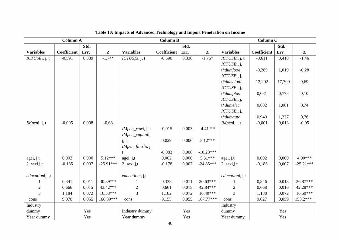
40

Table 10: Impacts of Advanced Technology and Import Penetration on Income

Column A Column B Column C

Variables Coefficient

Std.

Err. Z Variables Coefficient

Std.

Err. Z Variables Coefficient

Std.

Err. Z

ICTUSEi, j, t -0,591 0,339 -1.74* ICTUSEi, j, t -0,590 0,336 -1.76* ICTUSEi, j, t -0,611 0,418 -1,46

ICTUSEi, j,

t*dumfood -0,289 1,019 -0,28

ICTUSEi, j,

t*dumcloth 12,202 17,709 0,69

ICTUSEi, j,

t*dumplas 0,081 0,778 0,10

ICTUSEi, j,

t*dumelec 0,802 1,081 0,74

ICTUSEi, j,

t*dumauto 0,940 1,237 0,76

IMpeni, j, t -0,005 0,008 -0,68 IMpeni, j, t -0,001 0,013 -0,05

IMpen_rawi, j, t -0,015 0,003 -4.41***

IMpen_capitali,

j, t 0,029 0,006 5.12***

IMpen_finishi, j,

t -0,083 0,008 -10.23***

agei, j,t 0,002 0,000 5.12*** agei, j,t 0,002 0,000 5.31*** agei, j,t 0,002 0,000 4.90***

2. sexi,j,t -0,185 0,007 -25.91*** 2. sexi,j,t -0,178 0,007 -24.85*** 2. sexi,j,t -0,186 0,007 -25.21***

educationi, j,t educationi, j,t educationi, j,t

1 0,341 0,011 30.89*** 1 0,338 0,011 30.63*** 1 0,346 0,013 26.87***

2 0,666 0,015 43.42*** 2 0,661 0,015 42.84*** 2 0,668 0,016 42.28***

3 1,184 0,072 16.53*** 3 1,182 0,072 16.40*** 3 1,188 0,072 16.50***

_cons 9,070 0,055 166.39*** _cons 9,155 0,055 167.77*** _cons 9,027 0,059 153.2***

Industry

dummy Yes Industry dummy Yes

Industry

dummy Yes

Year dummy Yes Year dummy Yes Year dummy Yes

41

Number of

obs 42.806 Number of obs 42.746

Number of

obs 42.806

Wald chi2(33) 7140,17 Wald chi2(33) 7592,87 Wald chi2(33) 6949,41

Prob > chi2 0,00 Prob > chi2 0,00 Prob > chi2 0,00

R-squared 0,182 R-squared 0,186 R-squared 0,1354

Root MSE 0,694 Root MSE 0,693 Root MSE 0,71396

Column D Column E Column F

Variables Coefficient

Std.

Err. Z Variables Coefficient

Std.

Err. Z Variables Coefficient

Std.

Err. Z

roboti, j, t -0,121 0,256 -0,47 roboti, j, t -0,187 0,257 -0,73 roboti, j, t 3,691 2,738 1,35

roboti, j,

t*dumfood -1,745 1,204 -1,45

roboti, j,

t*dumcloth

roboti, j,

t*dumplas -3,380 2,494 -1,36

roboti, j,

t*dumelec -3,317 2,409 -1,38

roboti, j,

t*dumauto -3,467 2,550 -1,36

IMpeni, j, t -0,013 0,009 -1,45 IMpeni, j, t -0,013 0,008 -1,59

IMpen_rawi, j, t -0,006 0,003 -1.82*

IMpen_capitali,

j, t 0,027 0,006 4.42***

IMpen_finishi, j,

t -0,070 0,009 -8.11***

agei, j,t 0,003 0,000 8.30*** agei, j,t 0,003 0,000 8.3*** agei, j,t 0,003 0,000 8.18***

2. sexi,j,t -0,180 0,008 -24.02*** 2. sexi,j,t -0,176 0,007 -23.41*** 2. sexi,j,t -0,180 0,008 -24.00***

educationi, j,t educationi, j,t educationi, j,t

1 0,342 0,011 30.26*** 1 0,340 0,011 30.08*** 1 0,342 0,011 30.10***

2 0,655 0,016 41.36*** 2 0,651 0,016 40.86*** 2 0,656 0,016 41.45***

3 1,166 0,074 15.70*** 3 1,166 0,075 15.57*** 3 1,167 0,074 15.74***

42

_cons 9,280 0,050 185.56*** _cons 9,305 0,050 184.74*** _cons 9,139 0,114 80.05***

Industry

dummy Yes Industry dummy Yes

Industry

dummy Yes

Year dummy Yes Year dummy Yes Year dummy Yes

Number of

obs 38.386 Number of obs 38.326

Number of

obs 38.386

Wald chi2(33) 6303,37 Wald chi2(33) 6594,14 Wald chi2(33) 6660,64

Prob > chi2 0,00 Prob > chi2 0,00 Prob > chi2 0,00

R-squared 0,1842 R-squared 0,186 R-squared 0,180

Root MSE 0,691 Root MSE 0,690 Root MSE 0,692

Column G Column H Column I

Variables Coefficient

Std.

Err. Z Variables Coefficient

Std.

Err. Z Variables Coefficient

Std.

Err. Z

ecommercei, j,

t 0,889 0,376 2.37** ecommercei, j, t 0,903 0,376 2.40**

ecommercei,

j, t 0,357 0,356 1,00

ecommercei,

j, t*dumfood -6,384 10,073 -0,63

ecommercei,

j, t*dumcloth -3,018 2,220 -1,36

ecommercei,

j, t*dumplas -57,800 15,946 -3.62***

ecommercei,

j, t*dumelec -5,663 2,562 -2.21**

ecommercei,

j, t*dumauto -3,109 1,575 -1.97**

IMpeni, j, t -0,008 0,008 -0,98 IMpeni, j, t -0,014 0,008 -1.66*

IMpen_rawi, j, t 0,001 0,003 0,17

IMpen_capitali,

j, t 0,011 0,005 2.10**

IMpen_finishi, j,

t -0,073 0,008 -8.67***

agei, j,t 0,003 0,000 9.06*** agei, j,t 0,003 0,000 9.13*** agei, j,t 0,003 0,000 9.00***

2. sexi,j,t -0,165 0,007 -22.67*** 2. sexi,j,t -0,160 0,007 -22.04*** 2. sexi,j,t -0,167 0,007 -22.53***

43

educationi, j,t educationi, j,t educationi, j,t

1 0,354 0,010 36.68*** 1 0,352 0,010 36.44*** 1 0,353 0,010 35.39***

2 0,685 0,015 45.33*** 2 0,682 0,015 44.92*** 2 0,684 0,015 44.53***

3 1,226 0,067 18.36*** 3 1,223 0,067 18.31*** 3 1,240 0,067 18.39***

_cons 9,052 0,024 380.63*** _cons 9,103 0,025 366.21*** _cons 9,010 0,027 337.67***

Industry

dummy Yes Industry dummy Yes

Industry

dummy Yes

Year dummy Yes Year dummy Yes Year dummy Yes

Number of

obs 23.571 Number of obs 23.540

Number of

obs 23.571

Wald chi2(33) 6985,33 Wald chi2(33) 7085,81 Wald chi2(33) 6956,02

Prob > chi2 0,00 Prob > chi2 0,00 Prob > chi2 0,00

R-squared 0,278 R-squared 0,280 R-squared 0,260

Root MSE 0,524 Root MSE 0,523 Root MSE 0,531

Notes: (1) For sex = ‘1’ represents male whilst ‘2’ represents female. (2) Education is composed of four ranks: ‘0’ represents lower or equal to primary education; ‘1’, lower secondary education; ‘2’, upper secondary

and post-secondary education; ‘3’, bachelor’s degree and higher. (3) All proxies of technology and import penetration are in logarithm. (4) ***, **, and * represent 1%, 5%, and 10% significant level, respectively.

Source: Authors’ calculation.

44

6. Conclusions and Policy Implications

This paper examines the impacts of advanced technology on a possible change in

workers’ skills and wages and on the possibility of workers becoming unemployed due to such

technological advancement. In addition, to confirm the effects of technological advancement

on wage/income, a wage equation at the individual level is performed over time using

information of the whole manufacturing sector and an individual sector. This study is different

from others in that technological advancements are proxied by three key aspects according to

their involvements in supply chains, i.e. ICT use, e-commerce (for both inbound and

outbound), and internal production (e.g. factory automation/robots). It compares the effects of

technological advancements on labour market outcomes with import penetration, delineated

into raw materials, capital goods, and final products.

Our results show that in Thailand, the impact of advanced technology in pushing

workers out of the job market is limited. Instead, it tends to affect the reallocation of workers

between skilled and unskilled positions. The results vary amongst proxies of technology and

sectors. Amongst the three proxies of advanced technology, e-commerce tends to positively

impact employment status, especially with the higher probability of workers shifting from

unskilled to skilled positions. Workers in the clothing and textile, food and beverage, and

electronics and machinery sectors tend to receive greater benefits from using e-commerce in

the supply chains than those in automotive and plastics and chemicals. On the impacts of

wage/income induced by e-commerce, our results reveal that wage/income tends to increase

only in the clothing and textile and food and beverage sectors whilst it tends to decline in the

plastics and chemicals and automotive and electronics sectors.

In contrast to e-commerce, ICT use negatively impacts employment status, especially

in lowering the probability of workers shifting from skilled to unskilled positions. The negative

impacts are found in relatively high capital-intensive industries, including automotive, plastics

and chemicals, and electronics and machinery. the impacts of intensity of robot use on

employment status/income changes emerge only when individual sectors are analysed.

Workers in the automotive and electronics and the plastics and chemical sectors tend to get

net negative impacts from the introduction of more robots. The intensity of robot use has less

severe effects on the food and beverage sector. Wage/income tends to adjust lower from an

increase in ICT use whilst introduction of more robots has a negative but statistically

insignificant impact on income.

Comparing the effects of technological advancement and import penetration, our results

show less concern for negative impacts induced by imports on employment status, particularly

imports of capital and raw materials. By contrast, concerns on employment status is uncovered

45

in imports of final products. Particularly, such imports could shift workers from skilled to

unskilled positions and reduce the probability of workers staying at the same job and receiving

higher income. Imports of final products dampen the wage/income of workers significantly.

Imports of raw materials also negatively impact wage/income but only when ICT use and

robots are proxies of technology. However, a negative effect of wage/income induced by

import penetration is far lower than that of technological advancement.

Three policy inferences are drawn from our study. First, the reallocation of workers is

unavoidable in response to technological advancement. In addition to supporting skill

improvement of workers, government should act as facilitator to vigorously reduce friction in

the labour market and smoothen the transitions of workers from one place to another.

Cooperation with private firms is necessary to manage information well – especially that

relating to job creation and destruction across firms and industries – and lessen friction in the

labour market. Attention should be paid more on capital-intensive industries where higher

negative impacts of advanced technology are revealed. Second, wage/income should be

properly adjusted by skill improvement. From our study, advanced technology helps workers

shift from relatively unskilled to skilled positions in some cases, but such benefits fall on

workers whose wage/income does not adjust along with skill improvement. Proper payment

schemes, beyond relying on minimum wage, could be developed to fairly treat workers, along

with encouraging them to improve skills and be flexible. Third, trade liberalisation could

continue in Thailand with less concern on labour market outcomes, as some developed

countries worry about, especially in terms of capital goods and raw materials. Although

liberalisation in final products could reduce the probability of workers shifting from unskilled

to skilled positions, they create a higher probability of bringing unemployed workers back into

the job market. The impacts of dampened wage/income induced by imports are minimal,

compared to those of technological advancement.

46

References

Acemoglu, D. and D. Autor (2011), ‘Skills, Tasks and Technologies: Implications for

Employment and Earnings’, Handbook of Labor Economics, 4, pp.1043–171.

Acemoglu, D. and P. Restrepo (2017). ‘Robots and Jobs: Evidence from US Labour Market’,

NBER Working Paper No. 23285, Cambridge, MA: National Bureau of Economic

Research.

Acemoglu, D. and P. Restrepo (2018a), ‘The Race between Man and Machine: Implication of

Technology for Growth, Factor Shares, and Employment’, American Economic Review,

108(6), pp.1488–542.

Acemoglu, D. and P. Restrepo (2018b), ‘Artificial Intelligence, Automation and Work’, in

A.K. Agrawal, J. Gans, and A. Goldfarb (eds.), The Economics of Artificial Intelligence.

Chicago, IL: University of Chicago Press.

Acemoglu, D. and P. Restrepo (2019), ‘Automation and New Tasks: How Technology

Displaces and Reinstates Labor’, Journal of Economic Perspectives, 33(2), pp.3–30.

Amiti, M. and J. Konings (2007), ‘Trade Liberalization, Intermediate Inputs and Productivity:

Evidence from Indonesia’, American Economic Review, 95(5), pp.1611–38.

Arntz, M., T. Gregory, and U. Zierahn (2016), ‘The Risk of Automation for Jobs in OECD

Countries: A Comparative Analysis’, OECD Social, Employment and Migration

Working Papers No. 189, Paris: OECD Publishing.

http://dx.doi.org/10.1787/5jlz9h56dvq7-en.

Autor, D. and A. Salomons (2018), ‘Is Automation Labour Share – Displacing? Productivity

Growth, Employment and the Labour Share’, Brookings Papers on Economic Activity,

Spring 2018.

Autor, D., D. Dorn., and G.H. Hanson (2015), ‘Untangling Trade and Technology: Evidence

from Local Labour Market’, The Economic Journal, 125 (May), pp.621–46.

Autor, D., D. Dorn., and L.F. Katz (2017), ‘The Fall of the Labor Share and the Rise of

Superstar Firms’, NBER Working Paper No. 23396, Cambridge, MA: National Bureau

of Economic Research.

Autor, D., F. Levy, and R.J. Murnane (2003), ‘The Skill Content of Recent Technological

Change: An Empirical Exploration’, The Quarterly Journal of Economics, 118(4),

pp.1279–333.

Barbieri, L., M. Piva, and M. Vivarelli (2019), ‘R&D, Embodied Technological Change and

Employment: Evidence from Italian Microdata,’ Industrial and Corporate Change,

28(1), pp.203–18.

47

Bartel, A., C. Ichniowski, and K.S. Source (2007), ‘How Does Information Technology Affect

Productivity? Plant-Level Comparisons of Product Innovation, Process Improvement,

and Worker Skills’, The Quarterly Journal of Economics, 122(4), pp.1721–58.

Beaudry, P., M. Doms, and E. Lewis (2006), ‘Endogenous Skill Bias in Technology Adoption:

City-Level Evidence from the IT Revolution’, NBER Working Paper No. 12521,

Cambridge, MA: National Bureau of Economic Research.

Bessen, J., A. Goos, A. Salomons, and W. Berge (2019), ‘Automatic Reaction – What

Happened to Workers at Firms that Automate?’, CPB Discussion Paper, February, The

Hague: CPB Netherlands Bureau of Economic Policy Analysis.

Calvino, F. (2019), ‘Technological Innovation and the Distribution of Employment Growth:

A Firm-Level Analysis,’ Industrial and Corporate Change, 28(1), pp.177–202.

Cirera, X. and L. Sabetti (2019), ‘The Effects of Innovation on Employment in Developing

Countries: Evidence from Enterprise Surveys,’ Industrial and Corporate Change,

28(1), pp.161–76.

Crespi, G., E. Tacsir, and M. Pereira (2019), ‘Effects of Innovation on Employment in Latin

America,’ Industrial and Corporate Change, 28(1), pp.139–59.

Dauth, W., S. Findeisen, J. Suedekum, and N. Woessner (2018), ‘Adjusting to Robots:

Worker-Level Evidence’, Opportunity and Inclusive Growth Institute Working Paper

No. 13, Minneapolis: Federal Reserve Bank of Minneapolis.

Electronic Transactions Development Agency (ETDA) (various years) Value of e-Commerce

Survey in Thailand, Thailand

Ford, M. (2015), Rise of the Robots: Technology and the Threat of a Jobless Future. New

York: Basic Books.

Frey, C.B. and M.A. Osborne (2013), The Future of Employment: How Susceptible Are Jobs

to Computerization? Oxford: University of Oxford.

Frey, C.B. and M. Osborne (2017), ‘The Future of Employment: How Susceptible Are Jobs to

Computerisation?’, Technological Forecasting and Social Change, 114, pp.254–80.

Gaggl, P. and G.C. Wright (2017), ‘A Short-Run View of What Computers Do: Evidence from

a UK Tax Incentive’, Applied Economics, 9(3), pp.262–94.

Graetz, G. and G. Michaels (2018), ‘Robots at Work’, The Review of Economics and Statistics,

100(5), pp.753–68.

Harrison, R., J. Jaumandreu, J. Mairesse, and B. Peters (2014), ‘Does Innovation Stimulate

Employment? A Firm-level Analysis Using Comparable Micro-data from Four

European Countries’, International Journal of Industrial Organization, 35(C), pp.29–

43.

48

Hausman, J.A. and D. McFadden (1984), ‘Specification Tests for the Multinomial Logit

Model’, Econometrica, 52(5), pp.1377–98.

Hou, J., C. Huang, G. Licht, J. Mairesse, P. Mohnen, B. Mulkay, B. Peters, Y. Wu, Y. Zhao,

and F. Zhen (2019), ‘Does Innovation Stimulate Employment? Evidence from China,

France, Germany, and The Netherlands,’ Industrial and Corporate Change, 28(1),

pp.109–21.

International Federation of Robotics (IFR) (various issues), World Robotics: Industrial

Robots. Frankfurt: IFR

Jongwanich, J., and A. Kohpaiboon (2020), ‘Development of Investment Policy Framework

and Business Environment for Advancing the Digital Economy’, International Institute

for Trade and Development (ITD), Bangkok (in Thai).

Kohpaiboon, A. and J. Jongwanich (2019), ‘Structural Adjustment and International Migration

in the Thai Garment Industry: Revisit’, in N. Hatsukano (ed.), Rethinking Migration

Governance in the Mekong Region: From the Perspective of the Migrant Workers and

Their Employer, ERIA Research Project Report FY2017 no.19, Jakarta: ERIA and IDE-

JETRO, 96-127.

Mairesse, J. and Y. Wu (2019), ‘Impacts of Innovation, Export and Other Factors on Firm

Employment Growth in Chinese Manufacturing Industries,’ Industrial and Corporate

Change, 28(1), pp.123–38.

National Statistical Office (NSO) (various years), Labour Force Survey, Thailand

Office of the National Economic and Social Development Council (various years), Gross

Output, Thailand

Petrin, A. and K. Train (2010), ‘A Control Function Approach to Endogeneity in Consumer

Choice Models’, Journal of Marketing Research, 47(2), pp.3–13.

Sala-i-Martin, X., G. Doppelhofer, and R.I. Miller (2004), ‘Determinants of Long-Term

Growth: A Bayesian Averaging of Classical Estimates (BACE) Approach’, American

Economic Review, 94(4), pp.813–35.

UNCTAD (2017), World Investment Report 2017: Investment and the Digital Economy

Geneva: United Nations.

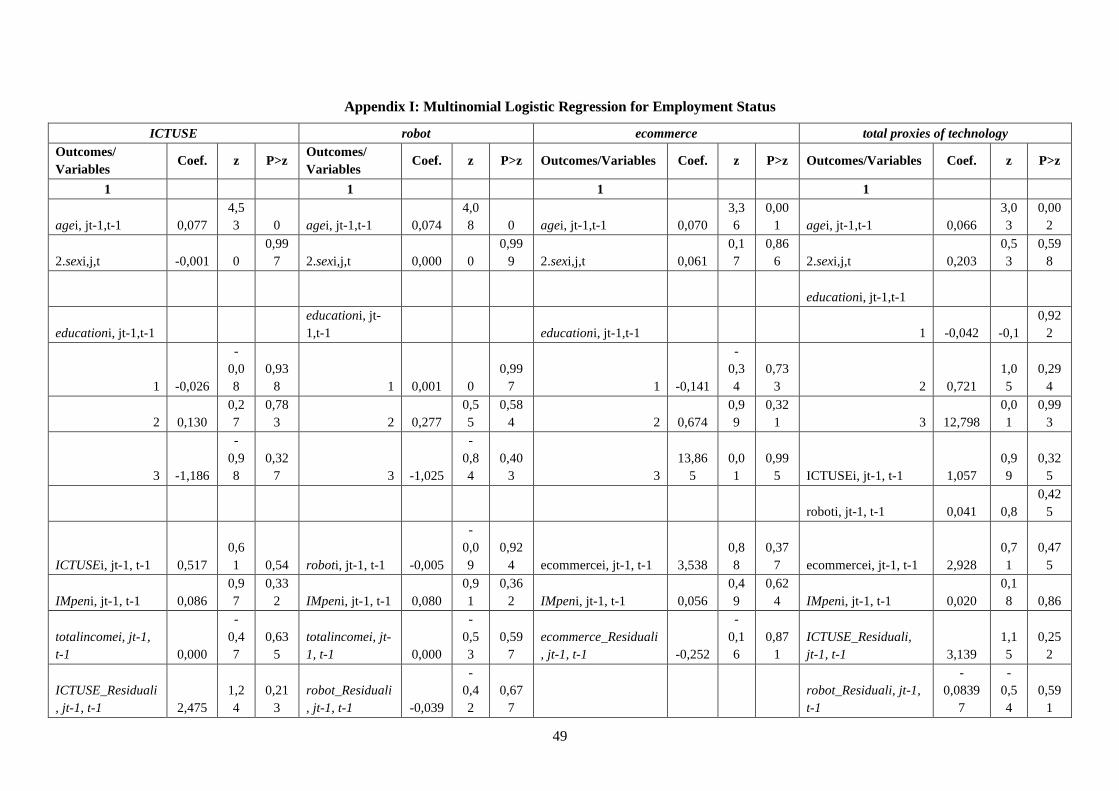
49

Appendix I: Multinomial Logistic Regression for Employment Status

ICTUSE robot ecommerce total proxies of technology

Outcomes/

Variables Coef. z P>z

Outcomes/

Variables Coef. z P>z Outcomes/Variables Coef. z P>z Outcomes/Variables Coef. z P>z

1 1 1 1

agei, jt-1,t-1 0,077

4,5

3 0 agei, jt-1,t-1 0,074

4,0

8 0 agei, jt-1,t-1 0,070

3,3

6

0,00

1 agei, jt-1,t-1 0,066

3,0

3

0,00

2

2.sexi,j,t -0,001 0

0,99

7 2.sexi,j,t 0,000 0

0,99

9 2.sexi,j,t 0,061

0,1

7

0,86

6 2.sexi,j,t 0,203

0,5

3

0,59

8

educationi, jt-1,t-1

educationi, jt-1,t-1

educationi, jt-

1,t-1 educationi, jt-1,t-1 1 -0,042 -0,1

0,92

2

1 -0,026

-

0,0

8

0,93

8 1 0,001 0

0,99

7 1 -0,141

-

0,3

4

0,73

3 2 0,721

1,0

5

0,29

4

2 0,130

0,2

7

0,78

3 2 0,277

0,5

5

0,58

4 2 0,674

0,9

9

0,32

1 3 12,798

0,0

1

0,99

3

3 -1,186

-

0,9

8

0,32

7 3 -1,025

-

0,8

4

0,40

3 3

13,86

5

0,0

1

0,99

5 ICTUSEi, jt-1, t-1 1,057

0,9

9

0,32

5

roboti, jt-1, t-1 0,041 0,8

0,42

5

ICTUSEi, jt-1, t-1 0,517

0,6

1 0,54 roboti, jt-1, t-1 -0,005

-

0,0

9

0,92

4 ecommercei, jt-1, t-1 3,538

0,8

8

0,37

7 ecommercei, jt-1, t-1 2,928

0,7

1

0,47

5

IMpeni, jt-1, t-1 0,086

0,9

7

0,33

2 IMpeni, jt-1, t-1 0,080

0,9

1

0,36

2 IMpeni, jt-1, t-1 0,056

0,4

9

0,62

4 IMpeni, jt-1, t-1 0,020

0,1

8 0,86

totalincomei, jt-1,

t-1 0,000

-

0,4

7

0,63

5

totalincomei, jt-

1, t-1 0,000

-

0,5

3

0,59

7

ecommerce_Residuali

, jt-1, t-1 -0,252

-

0,1

6

0,87

1

ICTUSE_Residuali,

jt-1, t-1 3,139

1,1

5

0,25

2

ICTUSE_Residuali

, jt-1, t-1 2,475

1,2

4

0,21

3

robot_Residuali

, jt-1, t-1 -0,039

-

0,4

2

0,67

7

robot_Residuali, jt-1,

t-1

-

0,0839

7

-

0,5

4

0,59

1

50

_cons 2,240

2,7

7

0,00

6 _cons 2,500

2,1

7 0,03 _cons 1,512

1,4

9

0,13

7

ecommerce_Residuali

, jt-1, t-1 0,154

0,0

8

0,93

9

_cons 1,363

1,0

2

0,30

6

2 2 2 2

agei, jt-1,t-1 0,108

6,3

8 0 agei, jt-1,t-1 0,104

5,7

9 0 agei, jt-1,t-1 0,101 4,9 0 agei, jt-1,t-1 0,095

4,3

9 0

2.sexi,j,t 0,105

0,3

7

0,71

3 2.sexi,j,t 0,162

0,5

3

0,59

5 2.sexi,j,t 0,174

0,4

8

0,63

1 2.sexi,j,t 0,340

0,8

9

0,37

6

educationi, jt-1,t-1

educationi, jt-1,t-1

educationi, jt-

1,t-1 educationi, jt-1,t-1 1 -0,056

-

0,1

3

0,89

7

1 -0,006

-

0,0

2

0,98

6 1 -0,006

-

0,0

2

0,98

6 1 -0,105

-

0,2

6

0,79

9 2 0,899

1,3

1 0,19

2 0,370

0,7

8

0,43

4 2 0,470

0,9

3

0,35

2 2 0,881 1,3

0,19

4 3 13,210

0,0

1

0,99

3

3 -0,594

-

0,4

9

0,62

2 3 -0,520

-

0,4

3 0,67 3

14,30

3

0,0

1

0,99

5 ICTUSEi, jt-1, t-1 1,212

1,1

3

0,25

8

roboti, jt-1, t-1 0,046 0,9 0,37

ICTUSEi, jt-1, t-1 0,538

0,6

4

0,52

2 roboti, jt-1, t-1 -0,014

-

0,2

9

0,77

5 ecommercei, jt-1, t-1 3,514

0,8

8 0,38 ecommercei, jt-1, t-1 3,218

0,7

8

0,43

2

IMpeni, jt-1, t-1 0,113

1,2

9

0,19

8 IMpeni, jt-1, t-1 0,109

1,2

4

0,21

5 IMpeni, jt-1, t-1 0,093

0,8

3

0,40

8 IMpeni, jt-1, t-1 0,063

0,5

6

0,57

3

totalincomei, jt-1,

t-1 0,000

-

0,8

8

0,37

9

totalincomei, jt-

1, t-1 0,000

-

0,7

6

0,44

5

ecommerce_Residuali

, jt-1, t-1 -0,401

-

0,2

6

0,79

5

ICTUSE_Residuali,

jt-1, t-1 2,560

0,9

4

0,34

9

ICTUSE_Residuali

, jt-1, t-1 2,490

1,2

5 0,21

robot_Residuali

, jt-1, t-1 -0,046

-

0,4

9

0,62

7

robot_Residuali, jt-1,

t-1 -0,073

-

0,4

7

0,63

8

51

_cons 1,792

2,2

2

0,02

6 _cons 1,665

1,4

4

0,14

9 _cons 1,001

0,9

9

0,32

4

ecommerce_Residuali

, jt-1, t-1 0,069

0,0

3

0,97

3

_cons 0,147

0,1

1

0,91

2

3 3 3 3

agei, jt-1,t-1 0,083

4,7

8 0 agei, jt-1,t-1 0,081

4,4

1 0 agei, jt-1,t-1 0,079

3,7

5 0 agei, jt-1,t-1 0,075

3,3

6

0,00

1

2.sexi,j,t 0,049

0,1

7

0,86

7 2.sexi,j,t 0,068

0,2

2

0,82

8 2.sexi,j,t 0,092

0,2

5

0,80

5 2.sexi,j,t 0,239 0,6

0,54

7

educationi, jt-1,t-1

educationi, jt-1,t-1

educationi, jt-

1,t-1 educationi, jt-1,t-1 1 0,298

0,6

6

0,50

9

1 0,171

0,4

9

0,62

3 1 0,169

0,4

5

0,64

9 1 0,284

0,6

6

0,50

9 2 1,480

2,1

1

0,03

5

2 0,843

1,7

5

0,08

1 2 0,962

1,8

7

0,06

2 2 1,500

2,1

7 0,03 3 13,441

0,0

1

0,99

3

3 -1,063

-

0,8

4 0,4 3 -0,912

-

0,7

1

0,47

5 3

14,68

4

0,0

1

0,99

5 ICTUSEi, jt-1, t-1 0,998

0,9

2

0,35

8

roboti, jt-1, t-1 0,032

0,5

8

0,55

9

ICTUSEi, jt-1, t-1 0,665

0,7

8

0,43

6 roboti, jt-1, t-1 -0,020

-

0,3

9 0,7 ecommercei, jt-1, t-1 2,947

0,7

3

0,46

6 ecommercei, jt-1, t-1 2,123

0,5

1

0,60

9

IMpeni, jt-1, t-1 0,089 1

0,31

8 IMpeni, jt-1, t-1 0,083

0,9

3

0,35

3 IMpeni, jt-1, t-1 0,072

0,6

2

0,53

4 IMpeni, jt-1, t-1 0,038

0,3

3

0,74

3

totalincomei, jt-1,

t-1 0,000

-

0,0

9

0,92

6

totalincomei, jt-

1, t-1 0,000

-

0,1

5

0,87

8

ecommerce_Residuali

, jt-1, t-1 -0,246

-

0,1

6

0,87

6

ICTUSE_Residuali,

jt-1, t-1 4,747

1,6

9

0,09

1

ICTUSE_Residuali

, jt-1, t-1 2,586 1,3

0,19

4

robot_Residuali

, jt-1, t-1 -0,036

-

0,3

8

0,70

6

robot_Residuali, jt-1,

t-1 -0,084

-

0,5

3

0,59

8

_cons -1,061

-

1,2

7

0,20

5 _cons 0,042

0,0

4

0,97

2 _cons -1,449

-

1,3

5

0,17

9

ecommerce_Residuali

, jt-1, t-1 0,165

0,0

8

0,93

6

52

_cons -1,142

-

0,8

2

0,41

1

4 4 4 4

agei, jt-1,t-1 0,095

5,4

6 0 agei, jt-1,t-1 0,092

5,0

1 0 agei, jt-1,t-1 0,095

4,4

7 0 agei, jt-1,t-1 0,092

4,1

3 0

2.sexi,j,t 0,228

0,7

8

0,43

7 2.sexi,j,t 0,300

0,9

5 0,34 2.sexi,j,t 0,289

0,7

7

0,44

4 2.sexi,j,t 0,477 1,2

0,23

1

educationi, jt-1,t-1

educationi, jt-1,t-1

educationi, jt-

1,t-1 educationi, jt-1,t-1 1 0,366

0,8

1 0,42

1 0,247

0,7

1 0,48 1 0,294

0,7

8

0,43

3 1 0,307

0,7

1

0,47

9 2 1,789

2,5

5

0,01

1

2 1,137

2,3

5

0,01

9 2 1,274

2,4

7

0,01

4 2 1,771

2,5

6

0,01

1 3 14,009

0,0

1

0,99

2

3 -0,191

-

0,1

5

0,87

8 3 -0,099

-

0,0

8

0,93

7 3

15,03

8

0,0

1

0,99

5 ICTUSEi, jt-1, t-1 0,639

0,5

8

0,56

1

roboti, jt-1, t-1 0,041

0,7

3

0,46

6

ICTUSEi, jt-1, t-1 0,011

0,0

1 0,99 roboti, jt-1, t-1 -0,006

-

0,1

2

0,90

4 ecommercei, jt-1, t-1 3,988

0,9

9 0,32 ecommercei, jt-1, t-1 3,429

0,8

3

0,40

4

IMpeni, jt-1, t-1 0,156

1,7

5 0,08 IMpeni, jt-1, t-1 0,150

1,6

9

0,09

1 IMpeni, jt-1, t-1 0,152

1,3

3

0,18

5 IMpeni, jt-1, t-1 0,121

1,0

6

0,28

9

totalincomei, jt-1,

t-1 0,000

0,2

4

0,80

7

totalincomei, jt-

1, t-1 0,000

0,2

6

0,79

8

ecommerce_Residuali

, jt-1, t-1 -0,462

-

0,2

9 0,77

ICTUSE_Residuali,

jt-1, t-1 2,754

0,9

8

0,32

8

ICTUSE_Residuali

, jt-1, t-1 2,408

1,2

1

0,22

7

robot_Residuali

, jt-1, t-1 -0,032

-

0,3

3

0,73

8

robot_Residuali, jt-1,

t-1 -0,059

-

0,3

7

0,70

9

_cons -1,130

-

1,3

5

0,17

6 _cons -1,082 -0,9

0,36

6 _cons -1,867

-

1,7

4

0,08

1

ecommerce_Residuali

, jt-1, t-1 -0,059

-

0,0

3

0,97

7

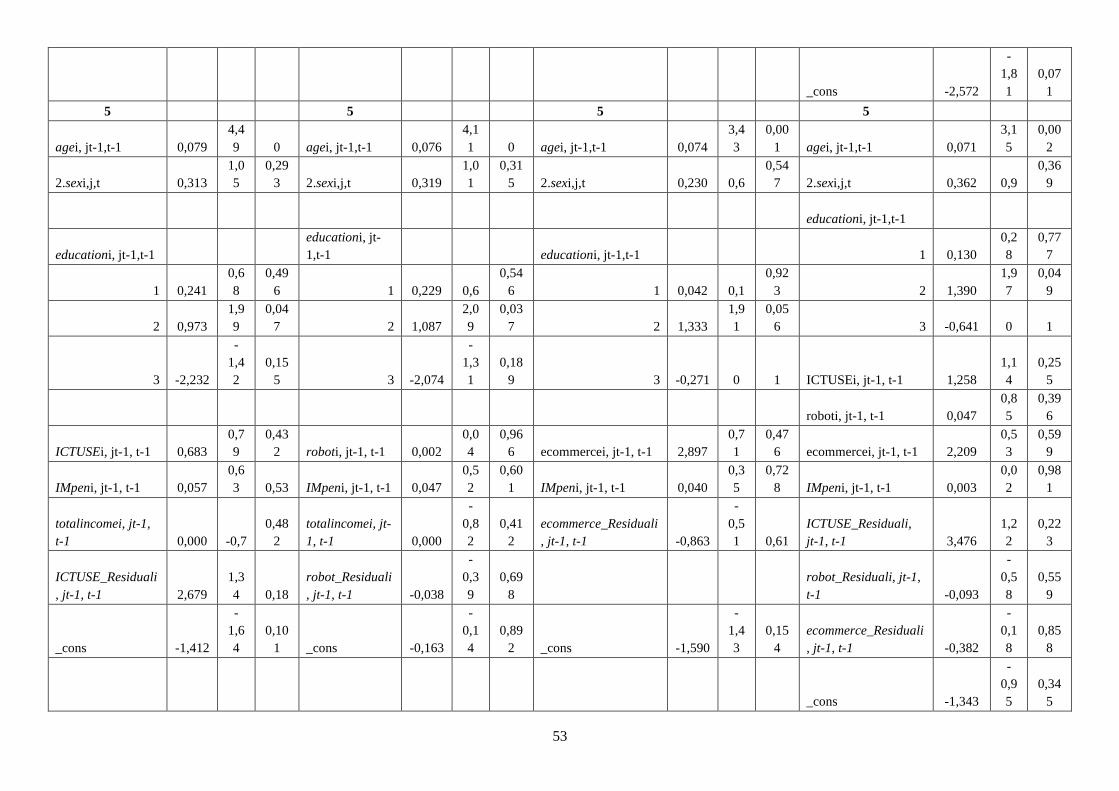
53

_cons -2,572

-

1,8

1

0,07

1

5 5 5 5

agei, jt-1,t-1 0,079

4,4

9 0 agei, jt-1,t-1 0,076

4,1

1 0 agei, jt-1,t-1 0,074

3,4

3

0,00

1 agei, jt-1,t-1 0,071

3,1

5

0,00

2

2.sexi,j,t 0,313

1,0

5

0,29

3 2.sexi,j,t 0,319

1,0

1

0,31

5 2.sexi,j,t 0,230 0,6

0,54

7 2.sexi,j,t 0,362 0,9

0,36

9

educationi, jt-1,t-1

educationi, jt-1,t-1

educationi, jt-

1,t-1 educationi, jt-1,t-1 1 0,130

0,2

8

0,77

7

1 0,241

0,6

8

0,49

6 1 0,229 0,6

0,54

6 1 0,042 0,1

0,92

3 2 1,390

1,9

7

0,04

9

2 0,973

1,9

9

0,04

7 2 1,087

2,0

9

0,03

7 2 1,333

1,9

1

0,05

6 3 -0,641 0 1

3 -2,232

-

1,4

2

0,15

5 3 -2,074

-

1,3

1

0,18

9 3 -0,271 0 1 ICTUSEi, jt-1, t-1 1,258

1,1

4

0,25

5

roboti, jt-1, t-1 0,047

0,8

5

0,39

6

ICTUSEi, jt-1, t-1 0,683

0,7

9

0,43

2 roboti, jt-1, t-1 0,002

0,0

4

0,96

6 ecommercei, jt-1, t-1 2,897

0,7

1

0,47

6 ecommercei, jt-1, t-1 2,209

0,5

3

0,59

9

IMpeni, jt-1, t-1 0,057

0,6

3 0,53 IMpeni, jt-1, t-1 0,047

0,5

2

0,60

1 IMpeni, jt-1, t-1 0,040

0,3

5

0,72

8 IMpeni, jt-1, t-1 0,003

0,0

2

0,98

1

totalincomei, jt-1,

t-1 0,000 -0,7

0,48

2

totalincomei, jt-

1, t-1 0,000

-

0,8

2

0,41

2

ecommerce_Residuali

, jt-1, t-1 -0,863

-

0,5

1 0,61

ICTUSE_Residuali,

jt-1, t-1 3,476

1,2

2

0,22

3

ICTUSE_Residuali

, jt-1, t-1 2,679

1,3

4 0,18

robot_Residuali

, jt-1, t-1 -0,038

-

0,3

9

0,69

8

robot_Residuali, jt-1,

t-1 -0,093

-

0,5

8

0,55

9

_cons -1,412

-

1,6

4

0,10

1 _cons -0,163

-

0,1

4

0,89

2 _cons -1,590

-

1,4

3

0,15

4

ecommerce_Residuali

, jt-1, t-1 -0,382

-

0,1

8

0,85

8

_cons -1,343

-

0,9

5

0,34

5

54

6 6 6 6

agei, jt-1,t-1 0,095

5,4

8 0 agei, jt-1,t-1 0,091

4,9

6 0 agei, jt-1,t-1 0,095

4,4

9 0 agei, jt-1,t-1 0,092

4,1

4 0

2.sexi,j,t 0,330

1,1

3

0,25

8 2.sexi,j,t 0,332

1,0

7

0,28

7 2.sexi,j,t 0,378

1,0

1

0,31

1 2.sexi,j,t 0,493

1,2

5

0,21

2

educationi, jt-1,t-1

educationi, jt-1,t-1

educationi, jt-

1,t-1 educationi, jt-1,t-1 1 0,235

0,5

2

0,60

1

1 -0,001 0

0,99

8 1 0,048

0,1

3

0,89

7 1 0,115

0,2

7

0,78

9 2 1,783

2,5

6

0,01

1

2 0,928

1,9

3

0,05

3 2 1,030

2,0

1

0,04

4 2 1,718 2,5

0,01

3 3 13,820

0,0

1

0,99

3

3 -1,102

-

0,8

9

0,37

5 3 -1,087

-

0,8

6

0,38

8 3

14,90

0

0,0

1

0,99

5 ICTUSEi, jt-1, t-1 0,903

0,8

3

0,40

6

roboti, jt-1, t-1 0,035

0,6

5

0,51

6

ICTUSEi, jt-1, t-1 0,308

0,3

6

0,71

9 roboti, jt-1, t-1 -0,018

-

0,3

6

0,71

7 ecommercei, jt-1, t-1 3,723

0,9

3

0,35

4 ecommercei, jt-1, t-1 3,079

0,7

5

0,45

4

IMpeni, jt-1, t-1 0,136

1,5

3

0,12

6 IMpeni, jt-1, t-1 0,133 1,5

0,13

4 IMpeni, jt-1, t-1 0,108

0,9

4

0,34

5 IMpeni, jt-1, t-1 0,080 0,7

0,48

3

totalincomei, jt-1,

t-1 0,000

0,8

5

0,39

7

totalincomei, jt-

1, t-1 0,000

0,8

4

0,40

4

ecommerce_Residuali

, jt-1, t-1 -0,405

-

0,2

6

0,79

7

ICTUSE_Residuali,

jt-1, t-1 3,870

1,3

9

0,16

5

ICTUSE_Residuali

, jt-1, t-1 2,130

1,0

7

0,28

6

robot_Residuali

, jt-1, t-1 -0,052

-

0,5

5

0,58

5

robot_Residuali, jt-1,

t-1 -0,087

-

0,5

5

0,58

4

_cons -1,254

-

1,5

1

0,13

2 _cons -0,453

-

0,3

8

0,70

1 _cons -1,474 -1,4

0,16

2

ecommerce_Residuali

, jt-1, t-1 -0,047

-

0,0

2

0,98

2

_cons -1,758

-

1,2

7

0,20

4

7 7 (base outcome 7 (base outcome 7 (base outcome

8 8 8 8

55

agei, jt-1,t-1 -0,021 -0,8

0,42

1 agei, jt-1,t-1 -0,025

-

0,9

1

0,36

1 agei, jt-1,t-1 -0,008

-

0,2

3

0,81

5 agei, jt-1,t-1 -0,012

-

0,3

6

0,71

9

2.sexi,j,t 0,247

0,5

5

0,58

5 2.sexi,j,t 0,395

0,8

3

0,40

7 2.sexi,j,t 0,293

0,5

4

0,58

9 2.sexi,j,t 0,436

0,7

8

0,43

4

educationi, jt-1,t-1

educationi, jt-1,t-1

educationi, jt-

1,t-1 educationi, jt-1,t-1 1 0,174

0,2

5 0,8

1 1,410

2,2

8

0,02

2 1 1,207 1,9

0,05

7 1 0,135 0,2

0,84

2 2 0,842

0,8

9

0,37

2

2 1,288

1,6

6

0,09

7 2 1,284 1,6

0,10

9 2 0,871

0,9

3

0,35

3 3 -0,013 0 1

3

-

11,78

4

-

0,0

2

0,98

5 3

-

11,62

1

-

0,0

2

0,98

3 3 0,283 0 1 ICTUSEi, jt-1, t-1 0,203

0,1

1

0,90

9

roboti, jt-1, t-1 0,015

0,1

7

0,86

5

ICTUSEi, jt-1, t-1 -0,721

-

0,4

8

0,63

3 roboti, jt-1, t-1 0,120

1,5

8

0,11

4 ecommercei, jt-1, t-1 1,495

0,3

2

0,75

2 ecommercei, jt-1, t-1 1,233

0,2

4

0,80

7

IMpeni, jt-1, t-1 -0,013

-

0,1

1

0,91

5 IMpeni, jt-1, t-1 -0,042

-

0,3

2

0,74

5 IMpeni, jt-1, t-1 0,112

0,7

6

0,44

7 IMpeni, jt-1, t-1 0,097

0,6

6

0,50

7

totalincomei, jt-1,

t-1 -0,001

-

5,8

8 0

totalincomei, jt-

1, t-1 -0,001

-

5,9

5 0

ecommerce_Residuali

, jt-1, t-1 -8,184

-

1,1

5

0,24

9

ICTUSE_Residuali,

jt-1, t-1 3,639

0,6

9

0,48

7

ICTUSE_Residuali

, jt-1, t-1 2,284

1,0

8

0,28

1

robot_Residuali

, jt-1, t-1 0,094

0,6

2

0,53

6

robot_Residuali, jt-1,

t-1 0,637

1,4

5

0,14

6

_cons 0,763

0,5

6

0,57

7 _cons 2,524

1,4

1

0,15

7 _cons

-

15,14

1

-

0,0

2

0,98

8

ecommerce_Residuali

, jt-1, t-1 -6,309

-

0,7

6

0,44

8

_cons -0,898

-

0,4

2

0,67

6

56

Industry dummy

for all outcomes Yes

Industry

dummy for all

outcomes Yes

Industry dummy for

all outcomes Yes

Industry dummy for

all outcomes Yes

Year dummy for

all outcomes Yes

Year dummy

for all outcomes Yes

Year dummy for all

outcomes Yes

Year dummy for all

outcomes Yes

Number of obs 16.275 Number of obs 14.252 Number of obs 9.344 Number of obs 8.820

LR chi2 2.372 LR chi2 2.043 LR chi2 963,35 LR chi2 950,56

Prob > chi2 0,00 Prob > chi2 0,00 Prob > chi2 0,00 Prob > chi2 0,00

Pseudo R2 0,0553 Pseudo R2 0,0534 Pseudo R2 0,0408 Pseudo R2 0,0425

Log likelihood -20255.424 Log likelihood -18107.519 Log likelihood -11310.391 Log likelihood -10708.156

Source: Authors’ estimation.

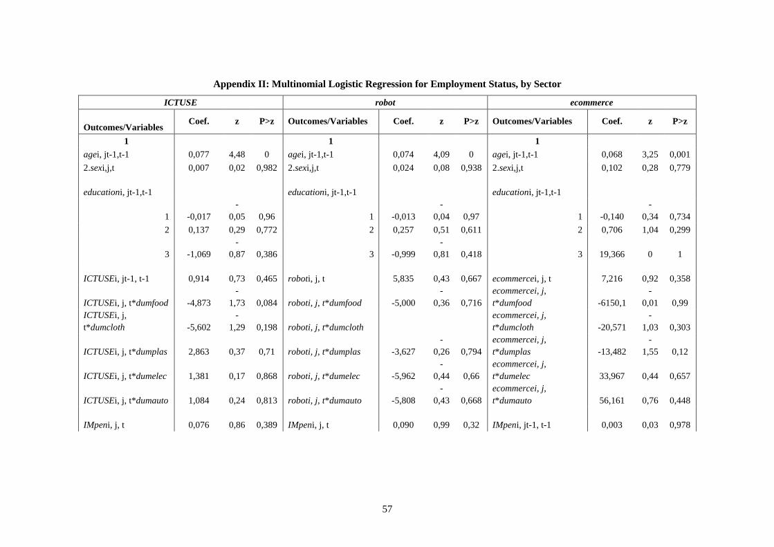
57

Appendix II: Multinomial Logistic Regression for Employment Status, by Sector

ICTUSE robot ecommerce

Outcomes/Variables Coef. z P>z Outcomes/Variables Coef. z P>z Outcomes/Variables Coef. z P>z

1 1 1

agei, jt-1,t-1 0,077 4,48 0 agei, jt-1,t-1 0,074 4,09 0 agei, jt-1,t-1 0,068 3,25 0,001

2.sexi,j,t 0,007 0,02 0,982 2.sexi,j,t 0,024 0,08 0,938 2.sexi,j,t 0,102 0,28 0,779

educationi, jt-1,t-1 educationi, jt-1,t-1 educationi, jt-1,t-1

1 -0,017

-

0,05 0,96 1 -0,013

-

0,04 0,97 1 -0,140

-

0,34 0,734

2 0,137 0,29 0,772 2 0,257 0,51 0,611 2 0,706 1,04 0,299

3 -1,069

-

0,87 0,386 3 -0,999

-

0,81 0,418 3 19,366 0 1

ICTUSEi, jt-1, t-1 0,914 0,73 0,465 roboti, j, t 5,835 0,43 0,667 ecommercei, j, t 7,216 0,92 0,358

ICTUSEi, j, t*dumfood -4,873

-

1,73 0,084 roboti, j, t*dumfood -5,000

-

0,36 0,716

ecommercei, j,

t*dumfood -6150,1

-

0,01 0,99

ICTUSEi, j,

t*dumcloth -5,602

-

1,29 0,198 roboti, j, t*dumcloth

ecommercei, j,

t*dumcloth -20,571

-

1,03 0,303

ICTUSEi, j, t*dumplas 2,863 0,37 0,71 roboti, j, t*dumplas -3,627

-

0,26 0,794

ecommercei, j,

t*dumplas -13,482

-

1,55 0,12

ICTUSEi, j, t*dumelec 1,381 0,17 0,868 roboti, j, t*dumelec -5,962

-

0,44 0,66

ecommercei, j,

t*dumelec 33,967 0,44 0,657

ICTUSEi, j, t*dumauto 1,084 0,24 0,813 roboti, j, t*dumauto -5,808

-

0,43 0,668

ecommercei, j,

t*dumauto 56,161 0,76 0,448

IMpeni, j, t 0,076 0,86 0,389 IMpeni, j, t 0,090 0,99 0,32 IMpeni, jt-1, t-1 0,003 0,03 0,978

58

totalincomei, jt-1, t-1 0,000

-

0,55 0,583 totalincomei, jt-1, t-1 0,000

-

0,62 0,533

ecommerce_Residuali,

jt-1, t-1 -0,982 -0,5 0,617

ICTUSE_Residuali, jt-

1, t-1 3,013 1,21 0,228

robot_Residuali, jt-1,

t-1 0,138 0,94 0,345

_cons 2,182 2,68 0,007 _cons 1,830 1,71 0,088 _cons 1,490 1,41 0,158

2 2 2

agei, jt-1,t-1 0,108 6,33 0 agei, jt-1,t-1 0,105 5,81 0 agei, jt-1,t-1 0,100 4,79 0

2.sexi,j,t 0,111 0,39 0,696 2.sexi,j,t 0,184 0,6 0,548 2.sexi,j,t 0,220 0,6 0,546

educationi, jt-1,t-1 educationi, jt-1,t-1 educationi, jt-1,t-1

1 0,006 0,02 0,987 1 -0,023

-

0,06 0,95 1 -0,099

-

0,24 0,81

2 0,381 0,81 0,42 2 0,449 0,89 0,374 2 0,918 1,35 0,176

3 -0,471

-

0,38 0,702 3 -0,502

-

0,41 0,683 3 19,807 0 1

ICTUSEi, jt-1, t-1 0,968 0,77 0,439 roboti, j, t 9,986 0,74 0,461 ecommercei, j, t 7,281 0,93 0,354

ICTUSEi, j, t*dumfood -6,162

-

2,19 0,029 roboti, j, t*dumfood -9,166

-

0,67 0,504

ecommercei, j,

t*dumfood -6138,4

-

0,01 0,99

ICTUSEi, j,

t*dumcloth -2,948

-

0,69 0,493 roboti, j, t*dumcloth

ecommercei, j,

t*dumcloth -27,718

-

1,39 0,164

ICTUSEi, j, t*dumplas 2,831 0,37 0,713 roboti, j, t*dumplas -7,899

-

0,57 0,568

ecommercei, j,

t*dumplas -10,396

-

1,21 0,227

ICTUSEi, j, t*dumelec 1,224 0,15 0,883 roboti, j, t*dumelec -10,111

-

0,75 0,455

ecommercei, j,

t*dumelec 45,304 0,59 0,553

ICTUSEi, j, t*dumauto 0,227 0,05 0,961 roboti, j, t*dumauto -9,972

-

0,74 0,461

ecommercei, j,

t*dumauto 50,175 0,68 0,498

IMpeni, j, t 0,102 1,16 0,245 IMpeni, j, t 0,122 1,34 0,179 IMpeni, jt-1, t-1 0,042 0,35 0,723

59

totalincomei, jt-1, t-1 0,000

-

0,95 0,342 totalincomei, jt-1, t-1 0,000

-

0,84 0,402

ecommerce_Residuali,

jt-1, t-1 -1,071

-

0,55 0,585

ICTUSE_Residuali, jt-

1, t-1 3,056 1,22 0,221

robot_Residuali, jt-1,

t-1 0,127 0,86 0,388

_cons 1,733 2,13 0,033 _cons 1,033 0,96 0,335 _cons 1,055 1 0,316

3 3 3

agei, jt-1,t-1 0,082 4,73 0 agei, jt-1,t-1 0,081 4,44 0 agei, jt-1,t-1 0,078 3,66 0

2.sexi,j,t 0,059 0,2 0,841 2.sexi,j,t 0,084 0,27 0,789 2.sexi,j,t 0,142 0,38 0,705

educationi, jt-1,t-1 educationi, jt-1,t-1 educationi, jt-1,t-1

1 0,177 0,51 0,609 1 0,154 0,41 0,679 1 0,290 0,67 0,501

2 0,847 1,75 0,079 2 0,939 1,83 0,068 2 1,547 2,23 0,025

3 -0,965

-

0,75 0,453 3 -0,878

-

0,68 0,494 3 20,190 0 1

ICTUSEi, jt-1, t-1 1,022 0,81 0,418 roboti, j, t 3,679 0,27 0,789 ecommercei, j, t 6,855 0,87 0,384

ICTUSEi, j, t*dumfood -4,433

-

1,52 0,129 roboti, j, t*dumfood -2,885

-

0,21 0,836

ecommercei, j,

t*dumfood -6156,4

-

0,01 0,99

ICTUSEi, j,

t*dumcloth -5,679

-

1,13 0,257 roboti, j, t*dumcloth

ecommercei, j,

t*dumcloth -30,464

-

1,35 0,175

ICTUSEi, j, t*dumplas 3,133 0,41 0,685 roboti, j, t*dumplas -0,574

-

0,04 0,967

ecommercei, j,

t*dumplas -10,214

-

1,16 0,245

ICTUSEi, j, t*dumelec 5,862 0,69 0,492 roboti, j, t*dumelec -3,789

-

0,28 0,783

ecommercei, j,

t*dumelec 33,248 0,43 0,668

ICTUSEi, j, t*dumauto -0,138

-

0,03 0,977 roboti, j, t*dumauto -3,679

-

0,27 0,789

ecommercei, j,

t*dumauto 55,038 0,74 0,46

IMpeni, j, t 0,083 0,92 0,355 IMpeni, j, t 0,087 0,94 0,346 IMpeni, jt-1, t-1 0,022 0,18 0,857

60

totalincomei, jt-1, t-1 0,000

-

0,18 0,857 totalincomei, jt-1, t-1 0,000

-

0,27 0,788

ecommerce_Residuali,

jt-1, t-1 -0,751

-

0,38 0,705

ICTUSE_Residuali, jt-

1, t-1 3,163 1,26 0,206

robot_Residuali, jt-1,

t-1 0,122 0,82 0,412

_cons -1,131

-

1,34 0,181 _cons -0,506

-

0,46 0,647 _cons -0,996

-

0,91 0,362

4 4 4

agei, jt-1,t-1 0,095 5,43 0 agei, jt-1,t-1 0,093 5,03 0 agei, jt-1,t-1 0,094 4,37 0

2.sexi,j,t 0,238 0,81 0,418 2.sexi,j,t 0,319 1,01 0,311 2.sexi,j,t 0,332 0,88 0,379

educationi, jt-1,t-1 educationi, jt-1,t-1 educationi, jt-1,t-1

1 0,254 0,73 0,467 1 0,276 0,74 0,461 1 0,311 0,72 0,472

2 1,146 2,37 0,018 2 1,253 2,43 0,015 2 1,806 2,6 0,009

3 -0,066

-

0,05 0,958 3 -0,077

-

0,06 0,952 3 20,528 0 1

ICTUSEi, jt-1, t-1 0,318 0,25 0,804 roboti, j, t 11,833 0,85 0,397 ecommercei, j, t 7,688 0,98 0,328

ICTUSEi, j, t*dumfood -4,129

-

1,41 0,159 roboti, j, t*dumfood -11,012

-

0,78 0,436

ecommercei, j,

t*dumfood -6127,5

-

0,01 0,99

ICTUSEi, j,

t*dumcloth 0,221 0,05 0,963 roboti, j, t*dumcloth

ecommercei, j,

t*dumcloth -31,967

-

1,41 0,158

ICTUSEi, j, t*dumplas 2,218 0,29 0,775 roboti, j, t*dumplas -9,381

-

0,66 0,511

ecommercei, j,

t*dumplas -8,922

-

1,02 0,307

ICTUSEi, j, t*dumelec 2,909 0,33 0,738 roboti, j, t*dumelec -11,940

-

0,86 0,393

ecommercei, j,

t*dumelec 30,698 0,39 0,695

ICTUSEi, j, t*dumauto 1,650 0,34 0,731 roboti, j, t*dumauto -11,815

-

0,85 0,398

ecommercei, j,

t*dumauto 44,676 0,59 0,552

IMpeni, j, t 0,148 1,67 0,095 IMpeni, j, t 0,163 1,78 0,075 IMpeni, jt-1, t-1 0,099 0,83 0,406

61

totalincomei, jt-1, t-1 0,000 0,2 0,84 totalincomei, jt-1, t-1 0,000 0,19 0,846

ecommerce_Residuali,

jt-1, t-1 -1,182

-

0,59 0,552

ICTUSE_Residuali, jt-

1, t-1 2,970 1,19 0,236

robot_Residuali, jt-1,

t-1 0,135 0,89 0,374

_cons -1,198

-

1,42 0,155 _cons -1,678

-

1,49 0,136 _cons -1,866 -1,7 0,089

5 5 5

agei, jt-1,t-1 0,078 4,43 0 agei, jt-1,t-1 0,077 4,15 0 agei, jt-1,t-1 0,072 3,34 0,001

2.sexi,j,t 0,316 1,06 0,29 2.sexi,j,t 0,332 1,04 0,297 2.sexi,j,t 0,280 0,73 0,465

educationi, jt-1,t-1 educationi, jt-1,t-1 educationi, jt-1,t-1

1 0,252 0,71 0,477 1 0,222 0,58 0,559 1 0,050 0,11 0,909

2 0,985 2,01 0,044 2 1,073 2,06 0,039 2 1,387 1,99 0,047

3 -2,061 -1,3 0,194 3 -2,024

-

1,28 0,202 3 -0,382 0 1

ICTUSEi, jt-1, t-1 1,303 1,03 0,305 roboti, j, t -3,460

-

0,25 0,806 ecommercei, j, t 6,421 0,81 0,416

ICTUSEi, j, t*dumfood -6,285

-

2,02 0,043 roboti, j, t*dumfood 4,336 0,3 0,761

ecommercei, j,

t*dumfood -6163,4

-

0,01 0,99

ICTUSEi, j,

t*dumcloth -14,273

-

2,16 0,031 roboti, j, t*dumcloth

ecommercei, j,

t*dumcloth -24,444

-

1,08 0,279

ICTUSEi, j, t*dumplas 1,281 0,17 0,869 roboti, j, t*dumplas 5,847 0,41 0,685

ecommercei, j,

t*dumplas -8,516

-

0,97 0,333

ICTUSEi, j, t*dumelec -5,330 -0,6 0,546 roboti, j, t*dumelec 3,408 0,24 0,809

ecommercei, j,

t*dumelec 0,229 0 0,998

ICTUSEi, j, t*dumauto 0,259 0,05 0,957 roboti, j, t*dumauto 3,472 0,25 0,806

ecommercei, j,

t*dumauto 66,718 0,9 0,369

IMpeni, j, t 0,042 0,47 0,641 IMpeni, j, t 0,043 0,46 0,645 IMpeni, jt-1, t-1 -0,010

-

0,08 0,937

62

totalincomei, jt-1, t-1 0,000

-

0,72 0,474 totalincomei, jt-1, t-1 0,000

-

0,95 0,342

ecommerce_Residuali,

jt-1, t-1 -1,299

-

0,63 0,528

ICTUSE_Residuali, jt-

1, t-1 3,235 1,29 0,197

robot_Residuali, jt-1,

t-1 0,158 1,05 0,295

_cons -1,444

-

1,67 0,096 _cons -0,612

-

0,54 0,589 _cons -1,118 -1 0,317

6 6 6

agei, jt-1,t-1 0,094 5,42 0 agei, jt-1,t-1 0,091 4,99 0 agei, jt-1,t-1 0,093 4,38 0

2.sexi,j,t 0,339 1,16 0,246 2.sexi,j,t 0,346 1,1 0,269 2.sexi,j,t 0,423 1,13 0,258

educationi, jt-1,t-1 educationi, jt-1,t-1 educationi, jt-1,t-1

1 0,013 0,04 0,97 1 0,031 0,08 0,934 1 0,126 0,29 0,769

2 0,948 1,97 0,049 2 1,010 1,97 0,049 2 1,761 2,56 0,011

3 -0,950

-

0,75 0,452 3 -1,063

-

0,84 0,401 3 20,38 0 1

ICTUSEi, jt-1, t-1 0,734 0,58 0,562 roboti, j, t 14,457 1,04 0,298 ecommercei, j, t 7,144 0,91 0,363

ICTUSEi, j, t*dumfood -6,543

-

2,15 0,032 roboti, j, t*dumfood -13,664

-

0,97 0,331

ecommercei, j,

t*dumfood -6170,2

-

0,01 0,99

ICTUSEi, j,

t*dumcloth -8,986

-

1,66 0,098 roboti, j, t*dumcloth

ecommercei, j,

t*dumcloth -29,895

-

1,33 0,184

ICTUSEi, j, t*dumplas 2,231 0,29 0,773 roboti, j, t*dumplas -11,731

-

0,83 0,408

ecommercei, j,

t*dumplas -8,267

-

0,95 0,34

ICTUSEi, j, t*dumelec 3,943 0,46 0,646 roboti, j, t*dumelec -14,543

-

1,05 0,295

ecommercei, j,

t*dumelec 21,292 0,27 0,785

ICTUSEi, j, t*dumauto 2,801 0,6 0,549 roboti, j, t*dumauto -14,459

-

1,04 0,298

ecommercei, j,

t*dumauto 27,607 0,37 0,713

IMpeni, j, t 0,126 1,42 0,157 IMpeni, j, t 0,146 1,6 0,11 IMpeni, jt-1, t-1 0,056 0,47 0,637

63

totalincomei, jt-1, t-1 0,000 0,8 0,421 totalincomei, jt-1, t-1 0,000 0,78 0,433

ecommerce_Residuali,

jt-1, t-1 -1,128

-

0,57 0,57

ICTUSE_Residuali, jt-

1, t-1 2,717 1,08 0,278

robot_Residuali, jt-1,

t-1 0,103 0,69 0,49

_cons -1,302

-

1,55 0,12 _cons -0,979

-

0,89 0,374 _cons -1,355

-

1,25 0,212

7

(base

outcome) 7

(base

outcome) 7

(base

outcome)

8 8 8

agei, jt-1,t-1 -0,021

-

0,83 0,408 agei, jt-1,t-1 -0,026

-

0,95 0,341 agei, jt-1,t-1 -0,009

-

0,27 0,788

2.sexi,j,t 0,258 0,57 0,57 2.sexi,j,t 0,441 0,92 0,357 2.sexi,j,t 0,339 0,62 0,533

educationi, jt-1,t-1 educationi, jt-1,t-1 educationi, jt-1,t-1

1 1,438 2,32 0,02 1 1,165 1,84 0,066 1 0,097 0,14 0,886

2 1,277 1,63 0,102 2 1,221 1,52 0,129 2 0,871 0,93 0,354

3 -10,925

-

0,03 0,978 3 -10,922

-

0,03 0,979 3 0,276 0 1

ICTUSEi, jt-1, t-1 -0,820

-

0,39 0,696 roboti, j, t 16,296 0,58 0,56 ecommercei, j, t 7,267 0,91 0,363

ICTUSEi, j, t*dumfood 0,606 0,1 0,92 roboti, j, t*dumfood -16,015

-

0,57 0,568

ecommercei, j,

t*dumfood -6088

-

0,01 0,99

ICTUSEi, j,

t*dumcloth 11,307 1,22 0,221 roboti, j, t*dumcloth 0 (omitte

ecommercei, j,

t*dumcloth -10830

-

0,01 0,991

ICTUSEi, j, t*dumplas 10,495 0,99 0,323 roboti, j, t*dumplas -12,637

-

0,45 0,653

ecommercei, j,

t*dumplas -592,443 -0,7 0,484

ICTUSEi, j, t*dumelec 1,293 0,09 0,927 roboti, j, t*dumelec -15,978

-

0,57 0,568

ecommercei, j,

t*dumelec -56,367

-

0,52 0,603

64

ICTUSEi, j, t*dumauto -1,664

-

0,22 0,825 roboti, j, t*dumauto -16,179

-

0,58 0,563

ecommercei, j,

t*dumauto 14,797 0,17 0,863

IMpeni, j, t -0,006

-

0,05 0,961 IMpeni, j, t -0,071 -0,5 0,618 IMpeni, jt-1, t-1 0,044 0,29 0,772

totalincomei, jt-1, t-1 -0,001

-

5,88 0 totalincomei, jt-1, t-1 -0,001 -6 0

ecommerce_Residuali,

jt-1, t-1 -3,019

-

0,56 0,578

ICTUSE_Residuali, jt-

1, t-1 2,738 1,05 0,295

robot_Residuali, jt-1,

t-1 0,068 0,3 0,762

_cons 0,712 0,52 0,605 _cons 2,635 1,61 0,107 _cons -0,716

-

0,43 0,664

Industry dummy for all

outcomes Yes

Industry dummy for all

outcomes Yes

Industry dummy for all

outcomes Yes

Year dummy for all

outcomes Yes

Year dummy for all

outcomes Yes

Year dummy for all

outcomes Yes

Number of obs 16.275 Number of obs 14.169 Number of obs 9.344

LR chi2 2.426,36 LR chi2 2094 LR chi2 1.023

Prob > chi2 0,00 Prob > chi2 0,00 Prob > chi2 0,00

Pseudo R2 0,0566 Pseudo R2 0,0547 Pseudo R2 0,0434

Log likelihood -20228.191 Log likelihood -18082.257 Log likelihood -11280.568

Source: Authors’ estimation.

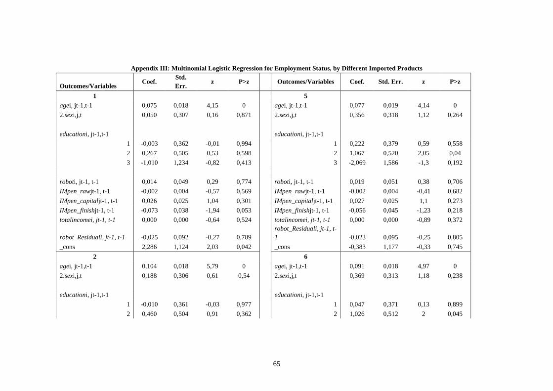
65

Appendix III: Multinomial Logistic Regression for Employment Status, by Different Imported Products

Outcomes/Variables Coef.

Std.

Err. z P>z Outcomes/Variables Coef. Std. Err. z P>z

1 5

agei, jt-1,t-1 0,075 0,018 4,15 0 agei, jt-1,t-1 0,077 0,019 4,14 0

2.sexi,j,t 0,050 0,307 0,16 0,871 2.sexi,j,t 0,356 0,318 1,12 0,264

educationi, jt-1,t-1 educationi, jt-1,t-1

1 -0,003 0,362 -0,01 0,994 1 0,222 0,379 0,59 0,558

2 0,267 0,505 0,53 0,598 2 1,067 0,520 2,05 0,04

3 -1,010 1,234 -0,82 0,413 3 -2,069 1,586 -1,3 0,192

roboti, jt-1, t-1 0,014 0,049 0,29 0,774 roboti, jt-1, t-1 0,019 0,051 0,38 0,706

IMpen_rawjt-1, t-1 -0,002 0,004 -0,57 0,569 IMpen_rawjt-1, t-1 -0,002 0,004 -0,41 0,682

IMpen_capitaljt-1, t-1 0,026 0,025 1,04 0,301 IMpen_capitaljt-1, t-1 0,027 0,025 1,1 0,273

IMpen_finishjt-1, t-1 -0,073 0,038 -1,94 0,053 IMpen_finishjt-1, t-1 -0,056 0,045 -1,23 0,218

totalincomei, jt-1, t-1 0,000 0,000 -0,64 0,524 totalincomei, jt-1, t-1 0,000 0,000 -0,89 0,372

robot_Residuali, jt-1, t-1 -0,025 0,092 -0,27 0,789

robot_Residuali, jt-1, t-

1 -0,023 0,095 -0,25 0,805

_cons 2,286 1,124 2,03 0,042 _cons -0,383 1,177 -0,33 0,745

2 6

agei, jt-1,t-1 0,104 0,018 5,79 0 agei, jt-1,t-1 0,091 0,018 4,97 0

2.sexi,j,t 0,188 0,306 0,61 0,54 2.sexi,j,t 0,369 0,313 1,18 0,238

educationi, jt-1,t-1 educationi, jt-1,t-1

1 -0,010 0,361 -0,03 0,977 1 0,047 0,371 0,13 0,899

2 0,460 0,504 0,91 0,362 2 1,026 0,512 2 0,045

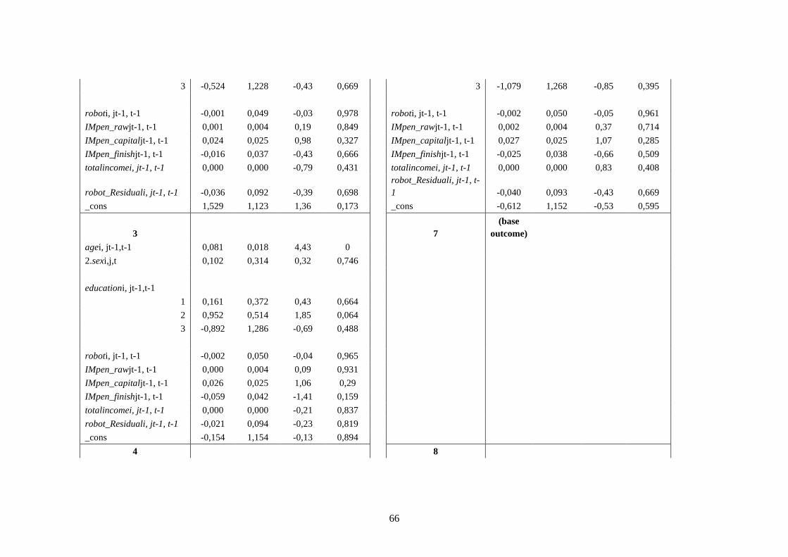
66

3 -0,524 1,228 -0,43 0,669 3 -1,079 1,268 -0,85 0,395

roboti, jt-1, t-1 -0,001 0,049 -0,03 0,978 roboti, jt-1, t-1 -0,002 0,050 -0,05 0,961

IMpen_rawjt-1, t-1 0,001 0,004 0,19 0,849 IMpen_rawjt-1, t-1 0,002 0,004 0,37 0,714

IMpen_capitaljt-1, t-1 0,024 0,025 0,98 0,327 IMpen_capitaljt-1, t-1 0,027 0,025 1,07 0,285

IMpen_finishjt-1, t-1 -0,016 0,037 -0,43 0,666 IMpen_finishjt-1, t-1 -0,025 0,038 -0,66 0,509

totalincomei, jt-1, t-1 0,000 0,000 -0,79 0,431 totalincomei, jt-1, t-1 0,000 0,000 0,83 0,408

robot_Residuali, jt-1, t-1 -0,036 0,092 -0,39 0,698

robot_Residuali, jt-1, t-

1 -0,040 0,093 -0,43 0,669

_cons 1,529 1,123 1,36 0,173 _cons -0,612 1,152 -0,53 0,595

3 7

(base

outcome)

agei, jt-1,t-1 0,081 0,018 4,43 0

2.sexi,j,t 0,102 0,314 0,32 0,746

educationi, jt-1,t-1

1 0,161 0,372 0,43 0,664

2 0,952 0,514 1,85 0,064

3 -0,892 1,286 -0,69 0,488

roboti, jt-1, t-1 -0,002 0,050 -0,04 0,965

IMpen_rawjt-1, t-1 0,000 0,004 0,09 0,931

IMpen_capitaljt-1, t-1 0,026 0,025 1,06 0,29

IMpen_finishjt-1, t-1 -0,059 0,042 -1,41 0,159

totalincomei, jt-1, t-1 0,000 0,000 -0,21 0,837

robot_Residuali, jt-1, t-1 -0,021 0,094 -0,23 0,819

_cons -0,154 1,154 -0,13 0,894

4 8

67

agei, jt-1,t-1 0,092 0,018 5,02 0 agei, jt-1,t-1 -0,023 0,027 -0,84 0,403

2.sexi,j,t 0,354 0,315 1,12 0,262 2.sexi,j,t 0,380 0,478 0,8 0,427

educationi, jt-1,t-1 educationi, jt-1,t-1

1 0,299 0,375 0,8 0,424 1 1,235 0,635 1,95 0,052

2 1,268 0,515 2,46 0,014 2 1,243 0,802 1,55 0,121

3 -0,073 1,264 -0,06 0,954 3 -10,892 408,890 -0,03 0,979

roboti, jt-1, t-1 0,017 0,051 0,33 0,744 roboti, jt-1, t-1 0,120 0,074 1,64 0,102

IMpen_rawjt-1, t-1 0,003 0,004 0,69 0,49 IMpen_rawjt-1, t-1 -0,010 0,007 -1,43 0,153

IMpen_capitaljt-1, t-1 0,029 0,025 1,18 0,239 IMpen_capitaljt-1, t-1 0,015 0,035 0,44 0,663

IMpen_finishjt-1, t-1 -0,068 0,043 -1,59 0,113 IMpen_finishjt-1, t-1 0,028 0,052 0,53 0,597

totalincomei, jt-1, t-1 0,000 0,000 0,22 0,828 totalincomei, jt-1, t-1 -0,001 0,000 -5,92 0

robot_Residuali, jt-1, t-1 -0,014 0,094 -0,15 0,88

robot_Residuali, jt-1, t-

1 0,095 0,148 0,64 0,523

_cons -1,291 1,171 -1,1 0,27 _cons 2,384 1,733 1,38 0,169

Industry dummy for all

outcomes Yes

Year dummy for all

outcomes Yes

Number of obs 14.151

LR chi2(126) 2128,26

Prob > chi2 0

Pseudo R2 0,0557

Log likelihood -18037.456

Note: Results of import penetration when ICTUSE or e-commerce used are the same as in the case of robots.

Source: Authors’ estimation.

ERIA Discussion Paper Series

No.  Author(s)  Title  Year

2020-08

(no. 335)

Duc Anh DANG, Thu

Thu VU

Technology Imports and Employment in

Developing Countries: Evidence from Viet

Nam

August

2020

2020-07

(no. 334)

Hiroaki ISHIWATA,

Hiroyuki WADA, Koji

SUZUKI, Makoto

IKEDA, Naoto TADA

A Quantitative Analysis of Disaster Risk

Reduction Investment Effects for

Sustainable Development: Indonesia Case

Study

June 2020

2020-06

(no. 333)

Dao Ngoc TIEN, Nguyen

Quynh HUONG

Assessment of Industrial Cluster Policies in

Viet Nam: The Role of Special Economic

Zones in Attracting Foreign Direct

Investment

June 2020

2020-05

(no. 332)

Ayako OBASHI,

Fukunari KIMURA

New Developments in International

Production Networks: Impact of Digital

Technologies

June 2020

2020-04

(no. 331)

Upalat

KORWATANASAKUL,

Youngmin BAEK,

Adam MAJOE

Analysis of Global Value Chain

Participation and the Labour Market in

Thailand:

A Micro-level Analysis

May 2020

2020-03

(no. 330)

Ha Thi Thanh DOAN,

Huong Quynh NGUYEN

Trade Reform and the Evolution of

Agglomeration

in Vietnamese Manufacturing

April 2020

2020-02

(no. 329)

Kazunobu HAYAKAWA,

Tadashi ITO, Shujiro

URATA

Labour Market Impacts of Import

Penetration from China and Regional Trade

Agreement Partners:

The Case of Japan

April 2020

2020-01

(no. 328)

Fukunari KIMURA,

Shandre Mugan

THANGAVELU,

Dionisius A. NARJOKO,

Christopher FINDLAY

Pandemic (COVID-19) Policy, Regional

Cooperation, and the Emerging Global

Production Network

April 2020

2019-41

(no. 327) Lurong CHEN

Improving Digital Connectivity For

E-commerce: A Policy Framework and

Empirical Note for ASEAN

March

2020

2019-40

(no. 326)

DAO Ngoc Tien and

Huong Qyunh NGUYEN

Tariff Policies and Wages in Manufacturing

Industries: New Evidence from Viet Nam

March

2020

2019-39

(no. 325)

Kazunobu HAYAKAWA,

Nuttawut

LAKSANAPANYAKUL,

Toshiyuki MATSUURA

Do Regional Trade Agreements Really Help

Global Value Chains Develop? Evidence

from Thailand

March

2020

2019-38

(no. 324)

Venkatachalam

ANBUMOZHI, Peter

WOLFF, Xianbin YAO

Policies and Financing Strategies for Low-

Carbon Energy Transition: Overcoming

Barriers to Private Financial Institutions

February

2020

2019-37

(no. 323) Deborah WINKLER

Global Value Chain Participation and the

Relative Demand for Skilled Labour in East

Asia

February

2020

69

2019-36

(no. 322)

Duc Anh DANG and Hai

Anh LA

The Effects of the Temporary Protection on

Firm Performance: Evidence from the Steel

Industry in Viet Nam

February

2020

2019-35

(no. 321) 

Kazunobu

HAYAKAWA, Hayato K

ATO, Toshiyuki

MATSUURA, Hiroshi

MUKUNOKI 

Production Dynamics in Multi-Product

Firms’ Exporting 

February

2020 

2019-34

(no. 320) 

Chin Hee

HAHN, Yong-Seok

CHOI 

Learning-to-Export Effect as a Response to

Export Opportunities: Micro-Evidence from

Korean Manufacturing 

February

2020 

2019-33

(no. 319) 

Samuel NURSAMSU,

Dionisius NARJOKO, 

Titik ANAS 

Input Allocation Behaviour on Tariff

Changes: The Case of Indonesia’s

Manufacturing Industries 

February

2020 

2019-32

(no. 318) 

Toshiyuki MATSUURA,

Hisamitsu SAITO 

Foreign Direct Investment and Labour

Market Dynamics in a Developing Country:

Evidence from Indonesian Plant-Level

Data 

February

2020 

2019-31

(no. 317) 

Nobuaki YAMASHITA,

Isamu YAMAUCHI 

Exports and Innovation: Evidence from

Antidumping Duties Against Japanese

Firms 

February

2020 

2019-30

(no. 316) 

Juthathip

JONGWANICH, 

Archanun 

KOHPAIBOON  

Effectiveness of Industrial Policy on Firms’

Productivity: Evidence from Thai

Manufacturing  

February

2020 

2019-29

(no. 315) 

Chin Hee HAHN, Ju

Hyun PYUN 

Does Home (Output) Import Tariff

Reduction Increase Home Exports?

Evidence from Korean Manufacturing

Plant–Product Data 

February

2020 

2019-28 

(no. 314) 

Thi Ha TRAN,

Quan Hoan

TRUONG, Van Chung

DONG 

Determinants of Product Sophistication in

Viet Nam: Findings from the Firm–Multi-

Product Level Microdata Approach 

February

2020 

2019-27 

(no. 313) 

Venkatachalam

ANBUMOZHI, Matthew

LOCASTRO, 

Dharish DAVID, Dian

LUTFIANA,

Tsani Fauziah 

RAKHMAH 

Unlocking the Potentials of Private

Financing for Low-carbon Energy

Transition: Ideas and Solutions from

ASEAN Markets 

January

2020 

2019-26

(no. 312) 

Takashi HONGO,

Venkatachalam

ANBUMOZHI 

Building the Banking Sector’s Capacity for

Green Infrastructure Investments for a Low-

Carbon Economy 

January 

2020 

2019-25

(no. 311) 

Peter A. PETRI,

Meenal BANGA 

The Economic Consequences of

Globalisation in the United States 

January 

2020 

2019-24 

(no. 310) 

Kaliappa

KALIRAJAN,

HUONG Thi Thu Tran,

Yochang LIU

Scalling up Private Investment in Low-

Carbon Energy Systems through Regional

Cooperation: Market-Based Trade Policy

Measures 

January

2020 

70

2019-23 

(no. 309)  VO Tri Thanh 

Enhancing Inter-Firm Linkages through

Clusters and Digitalisation for Productivity

Growth 

January

2020 

2019-22 

(no. 308) 

Archanun 

KOHPAIBOON,

Juthathip

JONGWANICH 

Economic Consequences of Globalisation:

Case Study of Thailand 

December

2019 

2019-21 

(no. 307)  Cassey LEE 

Globalisation and Economic

Development:  

Malaysia’s Experience 

December

2019 

2019-20 

(no. 306) 

Christopher FINDLAY,  

Kostas MAVROMARAS,

Zhang WEI 

Economic Consequences of Globalisation:

The Australian Framework for Reforms 

December

2019 

2019-19 

(no. 305) 

Md Abdullah AL

MATIN, Shutaro 

TAKEDA, Yugo

TANAKA, Shigeki

SAKURAI, Tetsuo

TEZUKA 

LCOE Analysis for Grid-Connected PV

Systems of Utility Scale Across Selected

ASEAN Countries 

November 

2019 

2019-18

(no. 304) 

Miaojie YU,  

Huihuang ZHU 

Processing Trade, Trade Liberalisation, and

Opening Up: China’s Miracle of

International Trade 

November

2019 

2019-17

(no. 303) 

Thanh Tri VO,  

Duong Anh NGUYEN,  

Thien Thi Nhan DO 

Economic Consequences of Trade and

Investment Liberalisation: The Case of Viet

Nam 

November

2019 

2019-16

(no. 302) 

Masahiko TSUTSUMI,

Masahito AMBASHI,

Asuna OKUBO

FTA Strategies to Strengthen Indonesian

Exports:  

Using the Computable General Equilibrium

Model 

November

2019 

2019-15 

(no. 301) 

Shujiro URATA,

Youngmin BAEK 

Does Participation in Global Value Chains

Increase Productivity? An Analysis of Trade

in Value Added Data 

November

2019 

2019-14

(no. 300)  Keiko ITO 

The Impact of Economic Globalisation on

Firm Performance and the Labour Market:

Evidence from Japan 

October

2019 

2019-13

(no. 299)  Markus NORNES 

Exporting ‘Content’ in the Face of

Indifference 

September

2019 

2019-12 

(no. 298) 

Trinh W. LONG, Matthias

HELBLE, Le T. TRANG 

Global Value Chains and Formal

Employment in Viet Nam 

September 

2019 

2019-11 

(no. 297) 

Makoto TOBA, Atul

KUMAR, Nuwong 

CHOLLACOOP, 

Soranan 

NOPPORNPRASITH, Ad

hika 

WIDYAPARAGA, Ruby

B. de GUZMAN,

Shoichi ICHIKAWA 

Evaluation of CO2 Emissions Reduction

through Mobility Electification 

September 

2019 

71

2019-10

(no.296)  Anne MCKNIGHT 

Words and Their Silos: Commercial,

Governmental, and Academic Support for

Japanese Literature and Writing Overseas 

August 

2019 

2019-09

(no.295)  Shinji OYAMA 

In the Closet: Japanese Creative Industries

and their Reluctance to Forge Global and

Transnational Linkages in ASEAN and East

Asia 

August 

2019 

2019-08

(no.294)  David LEHENY 

The Contents of Power: Narrative and Soft

Power in the Olympic Games Opening

Ceremonies 

August 

2019 

2019-07

(no.293)  DUC Anh Dang 

Value Added Exports and the Local Labour

Market: Evidence from Vietnamese

Manufacturing 

August 

2019 

2019-06

(no.292) 

Premachandra 

ATHUKORALA,

Arianto A. PATUNRU 

Domestic Value Added, Exports, and

Employment: An Input-Output Analysis of

Indonesian Manufacturing 

August 

2019 

2019-05

(no.291) 

Sasiwimon W.

PAWEENAWAT 

The Impact of Global Value Chain

Integration on Wages: Evidence from

Matched Worker-Industry Data in Thailand 

August 

2019 

2019-04

(no.290)  Tamako AKIYAMA 

A Spark Beyond Time and Place:

Ogawa Shinsuke and Asia 

August 

2019 

2019-03

(no.289) 

Naoyuki YOSHINO,

Farhad TARGHIZADEH-

HESARY 

Navigating Low-Carbon Finance

Management at Banks and Non-Banking

Financial Institutions 

August 

2019 

2019-02

(no.288)  Seio NAKAJIMA 

The Next Generation Automobile Industry

as a Creative Industry 

June 

2019 

2019-01

(no.287)  Koichi IWABUCHI 

Cool Japan, Creative Industries and

Diversity 

June 

2019 

ERIA discussion papers from the previous years can be found at: 

http://www.eria.org/publications/category/discussion-papers