Agricultural and Biosystems EngineeringConference Proceedings and Presentations Agricultural and Biosystems Engineering

7-2013

Techno-Economic Modeling of CoproductProcessing in a Corn Based Ethanol Plant in 2012Christine WoodSouth Dakota State University

Kurt A. RosentraterIowa State University, karosent@iastate.edu

Kasiviswanathan MuthukumarappanSouth Dakota State University

Follow this and additional works at: http://lib.dr.iastate.edu/abe_eng_conf

Part of the Agriculture Commons, and the Bioresource and Agricultural Engineering Commons

The complete bibliographic information for this item can be found at http://lib.dr.iastate.edu/abe_eng_conf/340. For information on how to cite this item, please visit http://lib.dr.iastate.edu/howtocite.html.

This Conference Proceeding is brought to you for free and open access by the Agricultural and Biosystems Engineering at Iowa State University DigitalRepository. It has been accepted for inclusion in Agricultural and Biosystems Engineering Conference Proceedings and Presentations by an authorizedadministrator of Iowa State University Digital Repository. For more information, please contact digirep@iastate.edu.

Techno-Economic Modeling of Coproduct Processing in a Corn BasedEthanol Plant in 2012

AbstractCoproducts, such as Distillers Dried Grains with Solubles (DDGS), produced during ethanol production areessential to the economic sustainability of each ethanol plant as they provide an additional source of revenue.DDGS is extensively used as animal feed, but has a relatively low market value compared to the biofuel. Byfractioning DDGS into lighter and heavier fractions, the overall composition changes potentially increasingthe value of the coproducts as they become more desirable to different markets. Earlier studies have examinedfractionating DDGS using sieves and aspirators. This project examined the techno-economics of addingfractionation systems onto an existing 40 million gal/y ethanol plant. The model allowed for estimations offixed capital costs, annual operating costs, annual revenues, and net profits, in order to determine theeconomic feasibility of adding three different fractionation systems. The first fractionation system consisted ofa single sieve, and the retained material was passed through an aspirator. The second system was similar to thefirst but with a second sieve and aspirator. The third system added a third set of them. In addition to utilizingdifferent fractionation systems, the scenarios examined the effects extracting corn oil and producing DWG inaddition to DDGS. The fractionation systems examined in this study increased the capital costs associatedwith the facility, but did not greatly affect the overall annual operating costs. The net profits in the four mostprofitable scenarios were $0.349/gal EtOH/y (scenario 14), $0.350/gal EtOH/y (scenarios 6 and 10), and$0.351/gal EtOH/y (scenario 2).

Keywordscorn, dry-grind, economics, ethanol, fractionation, DDGS, DWG, oil

DisciplinesAgriculture | Bioresource and Agricultural Engineering

This conference proceeding is available at Iowa State University Digital Repository: http://lib.dr.iastate.edu/abe_eng_conf/340

An ASABE Meeting Presentation

Paper Number: 131593363

Techno-Economic Modeling of Coproduct Processing in a Corn Based Ethanol Plant in 2012

Christine Wood1, Kurt A. Rosentrater2, Kasiviswanath Muthukumarappan3

1 Graduate Research Assistant, SDSU, Dept. of Agricultural and Biosystems Engineering,

SDSU North Campus Drive, Brookings, SD, 57006

2 Iowa State University, Dept. of Agricultural and Biosystems Engineering 3167 NSRIC, Ames, IA, 50011, karosent@iastate.edu

3 Professor, South Dakota State University, Dept. of Agricultural and Biosystems Engineering, SDSU North Campus Drive, Brookings, SD, 57007

Written for presentation at the 2013 ASABE Annual International Meeting

Sponsored by ASABE Kansas City, Missouri

July 21 – 24, 2013

Abstract. Coproducts, such as Distillers Dried Grains with Solubles (DDGS), produced during ethanol production are essential to the economic sustainability of each ethanol plant as they provide an additional source of revenue. DDGS is extensively used as animal feed, but has a relatively low market value compared to the biofuel. By fractioning DDGS into lighter and heavier fractions, the overall composition changes potentially increasing the value of the coproducts as they become more desirable to different markets. Earlier studies have examined fractionating DDGS using sieves and aspirators. This project examined the techno-economics of adding fractionation systems onto an existing 40 million gal/y ethanol plant. The model allowed for estimations of fixed capital costs, annual operating costs, annual revenues, and net profits, in order to determine the economic feasibility of adding three different fractionation systems. The first fractionation system consisted of a single sieve, and the retained material was passed through an aspirator. The second system was similar to the first but with a second sieve and aspirator. The third system added a third set of them. In addition to utilizing different fractionation systems, the scenarios examined the effects extracting corn oil and producing DWG in addition to DDGS. The fractionation systems examined in this study increased the capital costs associated with the facility, but did not greatly affect the overall annual operating costs. The net profits in the four most profitable scenarios were $0.349/gal EtOH/y (scenario 14), $0.350/gal EtOH/y (scenarios 6 and 10), and $0.351/gal EtOH/y (scenario 2).

Keywords. Corn; Dry-grind; Economics; Ethanol; Fractionation; DDGS; DWG; Oil

The authors are solely responsible for the content of this meeting presentation. The presentation does not necessarily reflect the official position of the American Society of Agricultural and Biological Engineers (ASABE), and its printing and distribution does not constitute an endorsement of views which may be expressed. Meeting presentations are not subject to the formal peer review process by ASABEeditorial committees; therefore, they are not to be presented as refereed publications. Citation of this work should state that it is from an ASABE meeting paper. EXAMPLE: Author's Last Name, Initials. 2013. Title of Presentation. ASABE Paper No. ---. St. Joseph, Mich.: ASABE. For information about securing permission to reprint or reproduce a meeting presentation, please contact ASABE atrutter@asabe.org or 269-932-7004 (2950 Niles Road, St. Joseph, MI 49085-9659 USA).

2

INTRODUCTION

In 2012 the U.S. ethanol industry produced 13.3 billion gallons of ethanol (RFA, 2012a).

Ethanol production begins with the breakdown of starches into useable sugars after the corn has

been processed either by wet milling or dry grind processing. The dry grind process, the

predominant method used within the ethanol industry today, grinds the corn, cooks and slurries

it, and then adds enzymes which transforms starch into simple sugars which can then be utilized

by yeast to produce ethanol (Singh et al., 2001).

In addition to the ethanol produced in 2012, the ethanol industry also produced a record 34.4

million metric tons of feed coproducts. These included corn gluten meal (CGM), corn gluten

feed (CGF), distillers dried grains with solubles (DDGS), and distillers wet grains (DWG) (RFA,

2013). These feed coproducts are comprised of the non-fermentable materials (i.e., proteins,

minerals, fats, and fibers) remaining after the starch is used to produce ethanol. CGM and CGF

are the products of the wet milling process, while the dry grind produces DWG and DDGS. Of

the feed coproduct produced, 92% was comprised of DDGS; this was an increase of nearly 32

million metric tons over 10 years (2001-2011) (RFA, 2012a and RFA, 2012b).

DDGS is composed of approximately 25% to 35% protein, 86.2% to 93.0% dry matter, 3% to

13% fat, and 7.2% fiber. This composition makes it ideal for feed (Bhadra et al., 2009b;

Ganesan et al., 2008; ISU, 2008; Rosentrater and Muthukumarappan, 2006; Shurson and

Alhamdi, 2008; Weigel et al., 1997). The livestock industry is currently the single largest

consumer of DDGS, utilizing 99% of the coproducts (RFA, 2012c). Of the 32.5 million metric

tons of DDGS in 2012, 79% was used for feeding cattle (beef and dairy) (compared to about 8%

3

for poultry and about 12% for swine) (RFA, 2013). The remaining 1% is used as fillers within

deicers, cat litter, lick barrels, and worm food (Bothast and Schlicher, 2005) or as feed

supplements for goats, sheep, and fish (RFA, 2012b; Kannadhason et al., 2010; Rosentrater et

al., 2009a; Rosentrater et al., 2009b; and Schaeffer et al., 2009). The fat and fiber content of

DDGS can limit the quantities in which it can be consumed by certain animals (Noll et al., 2011;

Shurson, 2002; and Tiffany et al., 2008).

If market saturation occurs, limited demand from the livestock industry may cause the supply of

DDGS to outgrow demand, if the production of DDGS continues to grow. To keep this from

happening, new value-added uses and new markets should be pursued to maintain the demand

for coproducts (Rosentrater, 2007). Some new potential uses for DDGS include ingredients

within the human food market (Rosentrater, 2007; Rosentrater and Krishnan, 2006), and fillers

for production of biodegradable plastics (Bothast and Schlicher, 2005; Tatara et al., 2006; Tatara

et al., 2007).

Another potential way of adding value to DDGS is to separate it into high protein fractions and

high fiber fractions. This approach will make more desirable product streams for various

industries. The high protein fraction (or low fiber fraction) would be more desirable for feed in

non-ruminant diets, while the high fiber fraction could be used for corn fiber gum, conversion

into cellulosic ethanol, and xylitol production (Srinivasan et al., 2005). This separation can be

achieved with the use of currently available technology, individual sieves (to separate DDGS

4

into size categories) and air (to separate based on mass density) (Srinivasan et al., 2005;

Srinivasan et al., 2009).

In addition to finding new markets for DDGS, the viability of new processes must be studied as

well. Most studies investigating new uses for DDGS and other coproducts are done on a small

scale (either bench top or pilot plants) and generally do not look into the economics of

processing at full scale. Alterations which may only be pennies at a bench top or pilot scale may

become hundreds or thousands of dollars under full commercial-scale processing conditions,

because economic inputs increase by several orders of magnitude. This can have a major effect

on the overall feasibility of the process. Thus, accurately predicting the cost of production prior

to adding a new technology to an existing, large-scale facility is crucial.

To determine the feasibility of a new process or system, economic predictions and planning for

resources, equipment capacities, and process parameters must be done. Computer based

modeling and simulations allow for these predictions to be readily made (Petrides et al., 2011).

Various industries, including pharmaceutical production and wastewater treatment, often use

computer-based models to simulate their processes (Akiyama et al., 2003; Prazeres et al., 2004;

Petrides et al., 1998; Petrides et al., 2002). The petrochemical industry began to use computer

models to simulate processes during the 1960’s in order to optimize production capacities

(Petrides et al., 2011), and the biofuels industry has recently begun following suit. For example,

ASPEN PLUS Software has been extensively used to simulate the transformation of corn into

ethanol, and to perform cost analysis of the production of biodiesel (Hass et al., 2006; McAloon

5

et al., 2000; Rajagopalan et al., 2004). The economic parameters for a typical 40 million gal/y

dry grind ethanol facility have also been determined with a corn ethanol plant model created in

SuperPro Designer (Intelligen, Inc., Scotch Plains, NJ) (Kwiatkowski et al., 2006).

The sensitivity of the Kwiatkowski et al., (2006) model to changes in raw material prices, market

prices, and coproduct processing operations (oil extraction, drying of DDGS, or producing

DWG) was subsequently explored by Wood et al., (2011), so that the model could then be

readily used to determine the economic feasibility of adding various new coproduct processing

steps to the plant. This study used the updated Kwiatkowski model (McAloon and Yee, 2011) to

determine the economic feasibility of adding a DDGS fractionation system on the end of an

existing dry-grind corn-ethanol plant. The objective of this study was to examine the techno-

economics of three different fractionation systems, consisting of combinations of sieves and

aspirators, onto the model used by Wood et al., (2011), and then to determine how effectively

they can add revenue versus additional expenses.

MATERIALS AND METHODS

Computer Model

Several years back, Kwiatkowski et al. (2006) created a 40 million gal/y ethanol plant model

using SuperPro Designer (Intelligen, Inc., Scotch Plains, NJ) that allowed process and economic

parameters of a real ethanol plant to be examined. The model was not based on a specific

ethanol plant, per se, but rather a generic dry grind plant that was comprised of all the individual

6

unit operations required to convert raw corn into ethanol. SuperPro Designer allows the

processing characteristics, capital and operation expenses for equipment, and economic

parameters to be defined, along with volumes, compositions, and physical characteristics for

each stream. It then uses the mass and economic balances for each of these individual unit

operations to determine overall balances for the entire process. This model was then updated in

by McAloon and Yee (2011) in order to reflect new ethanol processing technologies and current

economic values of equipment and materials. The sensitivity of this updated model was then

determined by Wood et al. (2012).

The model was configured to operate on the basis of 330 days/y, in order to reflect operation of a

real ethanol plant, which generally operates 24 h/day year round, with some scheduled down

time for maintenance and repairs. The processing characteristics, equipment parameters,

salaries, and utility, material, and equipment costs were updated from the original model based

on published materials and typical salaries in rural America in 2012. Additionally, in 2011,

McAloon and Yee added an oil extraction system and an option to extract DWG instead of

DDGS only to the Kwiatkowski et al., (2006) model. The information programed into the model

was then used by SuperPro Designer to produce a variety of output reports based on mass and

economic balances. These reports were generated for each simulation scenario in this study, and

then used to compare the economic feasibility and sensitivities of processing scenarios and

material prices.

7

Simulations

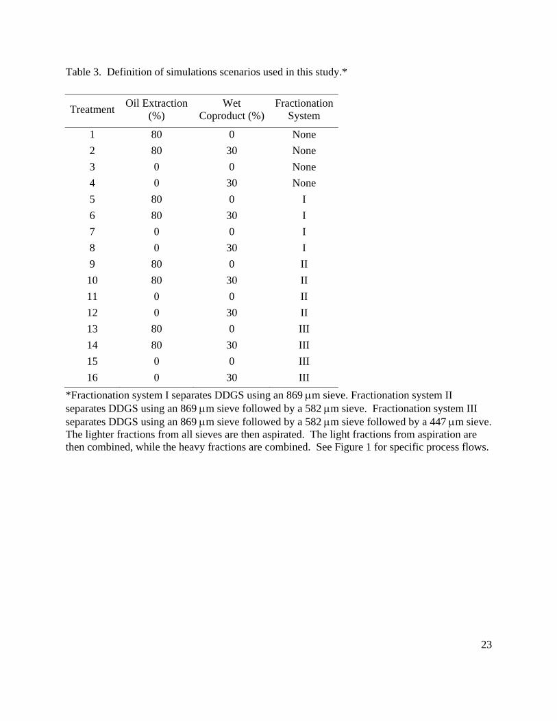
A series of simulations (Table 3) were run based on modifying how the coproducts were

processed (Figure 1). Three different variables were adjusted in the model:

1) quantity of oil extracted from condensed distillers solubles (CDS) (0% versus 80%);

2) quantity of distillers wet grains (DWG) produced (0% versus 30%);

3) type of fractionation system used to process distillers dried grains with solubles

(DDGS). One set of scenarios did not use fractionation, one used a combination of an 869 m

sieve and an aspirator, another used an 869 m sieve followed by a 582 m sieve and 2

aspirators, and another set used a combination of an 869 m sieve, 582 m sieve, and a 447 m

sieve, each followed by an aspirator. These combinations were based on preliminary

experimental work at our laboratory (not published). Fiber and protein composition and overall

mass balances of the DDGS streams were defined based upon data presented within Srinivasan et

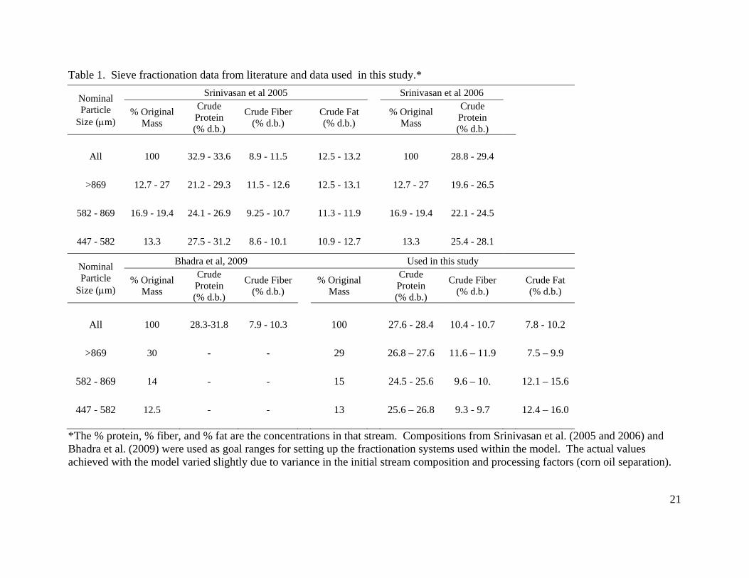
al., (2005, 2006) and Bhadra et al., (2009b). For example, these studies found that an 869 m

sieve would retain 12.7% to 30% of the streams mass, and the composition of that retained

stream would be 19.6% to 29.3% protein, 11.5% to 12.6% fiber, and 12.5% to 13.1% fat (Table

1); so these were the goal ranges used for setting up the fractionation system. The actual models

mass and compositional ranges (Table 1) varied slightly due to variance in the initial stream

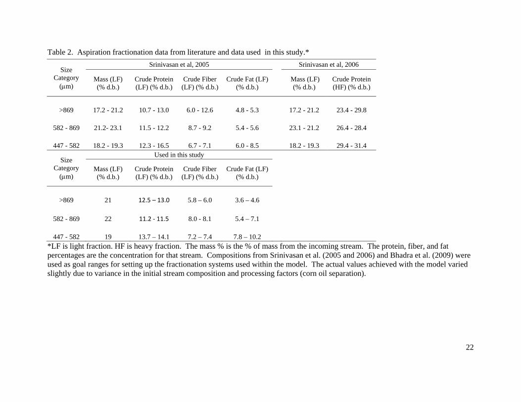
composition and due to processing factors (corn oil separation). Similarly the aspiration

separation was defined based upon Srinivasan et al., (2005, 2006) (Table 2). All of these were

data used as general guidelines when fractionating the simulated DDGS streams.

8

These three independent variables provided a total of sixteen independent production scenarios

for simulation (Table 3). For each simulation scenario, the direct fixed capital costs (DFC), the

annual operating costs (AOC), the annual revenue, coproduct composition, and the net profits

were computed. The fixed capital costs were sub divided into the various components that

comprise the entire facility: support systems, coproduct processing, ethanol processing,

fermentation, starch-to-sugar conversion, grain handling, and milling. The annual operating

costs were comprised of utilities, facilities, labor, and raw materials; utilities and materials were

broken down into individual components (e.g., electricity, cooling water, natural gas, steam,

corn, liquid ammonia, enzymes, sulfuric acid, yeast, etc.). Annual revenues were partitioned

according the products produced: ethanol, corn oil, DWG, DDGS, fractionated DDGS heavy

fraction (HF), and fractionated DDGS lighter fraction (LF).

RESULTS AND DISCUSSION

Capital Costs

Annualized direct fixed capital costs (DFC) were calculated based on the total equipment

purchase costs and maintenance cost (10% of purchase price) for the individual process sections

within the plant, including coproduct processing, support systems, ethanol processing,

fermentation, starch-to-sugar conversion, and grain handling/milling. Figure 2 illustrates the

DFC/gal of EtOH/y. The cost relationship of individual sections, as well as the overall operating

cost associated with each production scenario, can be found in Figure 2A. The DFC ranged

from $1.41-1.45/gal of EtOH/y ($56.0-57.7 million/y). Of the individual processing sections

9

used to determine the DFC, coproduct processing was the only one that varied between

scenarios. This can be seen in Figure 2B. The figure shows that coproduct processing costs

between $0.60-0.65/gal of EtOH/y ($24.1-25.7 million/y), which is approximately 43.7% of the

total capital costs for the ethanol plant. Coproduct processing costs twice as much per gallon of

ethanol as fermentation, and nearly 2.5 times as much per gallon as ethanol processing itself.

Based on this, it can be determined that, regardless of the presence or absence of fractionation

systems, coproduct processing comprises a significant portion of the capital costs associated due

to the ethanol plant.

Annual Operating Costs

In addition to the annualized capital costs associated with plant operations, the annual operating

costs (AOC) must be determined in order to do a complete techno-economic evaluation.

Expenses associated with the facilities, labor, materials, and utilities required for plant operation

comprised the total AOC of the ethanol facility. The relationships that these individual

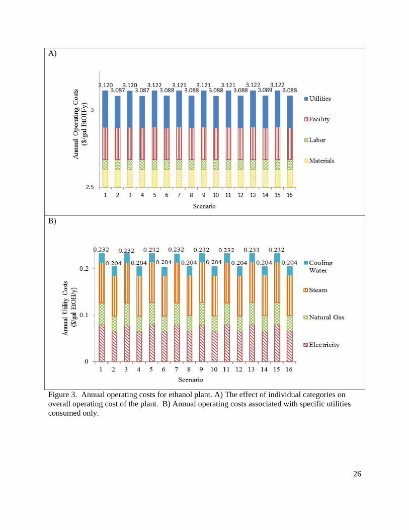
components have with each other, and the overall AOC, can be seen in Figure 3A. The total

AOC of the ethanol plant ranged from $3.09-3.12/gal of ethanol produced/y ($123.0-124.5

million/y). The cost of materials and labor remained constant between all sixteen scenarios,

while facilities and utilities were altered with changes in coproduct processing.

Utilities

10

Figure 3B illustrates the variation in the AOC associated with utilities only. It also shows

the relationship of the individual utilities with the overall costs. For the sixteen

production scenarios, utilities costs were $0.20-0.23/gal of EtOH/y ($8.0-9.0 million/y).

The quantity of the utilities used within the process (water, steam, gas, and electricity)

can be seen in Figure 4. The addition of various coproduct processing operations does

not affect the quantity of cooling water or the quantity of steam required annually; it did,

however, greatly impact the quantity of electricity required as well as the amount of

natural gas used. When more DWG was dried, more natural gas was required, while the

addition of fractionation systems increased the electrical requirements of the facility. The

facility utilized 0.98-1.20 kWh/gal of EtOH/y and 0.17-0.24 kg natural gas/gal of

EtOH/y.

Facilities

Facility costs included maintenance expenses, equipment depreciation, insurance, taxes,

and miscellaneous factory expenses. The cost of facilities ranged from $0.20-0.21/gal

EtOH/y ($8.1-8.4 million/y) for all sixteen scenarios. This small variation was due to the

addition of equipment for the fractionation systems and the increase of dryer capacities

when 100% of the DWG was dried onto DDGS.

Labor

11

The cost of labor was determined based upon a lump estimate of number of working

hours/y (330 day/y), and the median wage within the Midwest. For all sixteen scenarios

it was determined that labor cost contributed $2.5 million/y ($0.06/gal EtOH/y) to the

annual operating costs. This was approximately 2.0% of the AOC.

Material Cost

The vast majority of the annual operating cost comes from the raw materials

required. These materials cost approximately $2.62/gal of EtOH/y ($104.3 million/y;

84.3% of the AOC). Corn, octane, water, yeast, caustic, sulfuric acid, glucoamylase,

alpha amylase, liquid ammonia, and lime are the materials used within the model that

contribute to the material costs. Of these materials, corn plays the most significant role,

as it comprises 96% of the total material costs. For the simulations associated with this

study, the price of corn was set at $0.27/kg ($6.94/bushel) to reflect corn prices at the

time of simulation (DTN, 2013). Based on the quantity of corn utilized and ethanol

produced, this is equivalent to $2.52/gal of EtOH/y.

Annual Revenues

The ethanol production process followed in the model produced five products: carbon dioxide,

ethanol, corn oil, DWG, and DDGS (for some scenarios this was fractioned into light and heavy

fractions). For simplification, CO2 was not collected for resale or assigned a market value. The

12

other four products were used to determine the total annual revenue for the simulation. The

market prices for ethanol and oil were set to reflect market value at the time of simulation

($0.82/kg EtOH ($2.44/gal) (MN DOA,2012), $1.22/kg corn oil(USDA ERS, 2012)). The

market prices of DWG, DDGS, DDGS light fraction (LF), and DDGS heavy fraction (HF) were

left as variables and calculated by the computer model based upon their protein concentration.

The market value of protein ($1.05/ kg) was determined based upon the current market price of

DDGS ($240/ton (DTN, 2013)) with the assumption that DDGS is 25% protein.

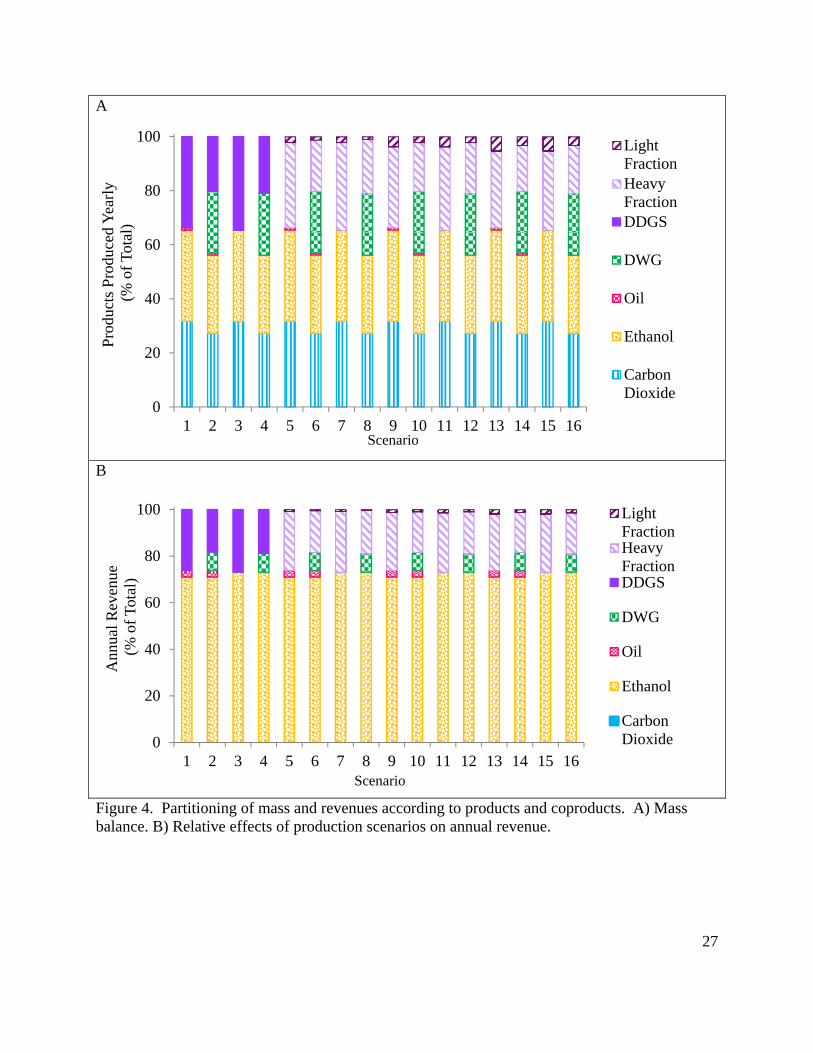
Figure 4 shows the effect that each of these products has on the revenue for the plant. Figure 4A

compares the annual quantity produced for each product, while part Figure 4B shows how each

product affects the overall annual revenue of the plant. The revenue produced ($/gal of EtOH/y)

is presented in Figure 5.

Ethanol

Ethanol was approximately 29-34% of the total mass produced annually by the ethanol

process (Figure 5B), but contributed 71-73% of the total annual revenue ($133-137

million/y) of the plant, as show Figure 5A.

Corn Oil

13

Corn oil produced revenue of $0.10/gal of EtOH/y ($3.9 million/y) in the scenarios where

80% of the oil was extracted. Figure 4A shows that when the 80% of the corn oil was

extracted (i.e. scenarios 1, 2, 5, 6, 9, 10, 13, and 14), the contribution of oil to plant

revenue was fairly low (2.86%) even though oil had the largest market price of all

products produced. This was due to the fact that its contribution to the total mass

produced was very minimal (0.78-0.91%) (Figure 4B).

DWG

The market value of DWG was determined based upon its protein concentration. For the

sixteen scenarios the price was $0.11/kg/y. In the scenarios where 30% of the DWG was

left wet, DWG made up approximately 23% of the mass produced by the plant (Figure

4B) and approximately 8% of the revenue (Figure 4A). DWG produced revenue of

$0.27/gal EtOH/y ($10.75 million/y).

DDGS

DDGS made up 20-35% of the total mass produced by the ethanol plant. Similar to the

DWG, the price of DDGS was set based upon protein content. The protein and fiber

content of the DDGS and the DDGS fractions can be found in Figure 6. The crude fiber

content for the whole DDGS ranged from 18.7% to 19.3%, while that of the light fraction

(LF) ranged from 5.9% to 7.2%, and that of the heavy fraction (HF) ranged from 19.6%

14

to 21.5% (Figure 6A). Figure 6B presents the protein concentration used to determine the

market value of the DDGS. The protein concentration of the whole DDGS was

determined to be 27.6% to 28.4%, in the FF was determined to be 12.2% to 13%, and in

the PF was determined to be 28.6% to 31.3%. Based on these protein concentrations,

whole DDGS had a market value of $0.29-0.30/kg ($0.14/ lb). The concentrations of

protein in the FF and PF varied greatly depending on the fractionation system used, and

therefore the market value of the product varied greatly. For scenarios 5-8, where one

sieve and one aspirator were used for separation, the FF had a market value of $0.14/kg

($0.06/lb) and the PF had a market value of $0.30-0.31/kg ($0.14/lb). When a second

sieve and aspirator were added to the system (scenarios 9-12), the market value of the FF

decreased to $0.13/ kg ($0.06/lb) and the value of the PF was increased to $0.31-0.32/ kg

($0.14/lb). The third fractionation system (scenarios 13-16), three sieves and three

aspirators, had a FF with a market value of $0.13/ kg ($0.06/lb) and a PF market value of

$0.32-0.33/ kg ($0.15/lb).

Net Profits

Figure 7A compares the DFC, AOC, and revenues to the net profits for the plant. The annual

profits ($/gal EtOH/y) can be found in Figure 7B. While all scenarios had positive profits, the

scenarios in which oil was extracted had significantly higher profits. Marketing DWG also

increased the profit margins. Scenario 2 had the greatest profit ($13.990 million/y), closely

followed by scenario 10 ($13.961 million/y), and then 6 ($13.956 million/y).

15

CONCLUSIONS

The ethanol production process results in a variety of products (in addition to ethanol) that can

provide additional revenue to the facility. The additional revenue streams can add to the profits

of the facility, as long as the cost of processing does not exceed revenues. In order to perform

economic calculations for new fractionation systems, SuperPro Designer was used for techno-

economic modeling. Through the simulated scenarios, it can be concluded that DDGS

fractionation has the potential to play a vital role in increasing the market value of the ethanol

coproducts. The fractionation systems incorporated in this study increased the capital costs

associated with the facility, but did not greatly affect the overall annual operating costs. The

scenarios where both DWG and DDGS were produced, in addition to the extraction of corn oil,

were the most profitable. The addition of fractionation added revenue and operating costs, and

improved the profits of the plant. Diversification of coproducts may be critical as the industry

continues to evolve.

REFERENCES

Akiyama, M., T. Tsuge, and Y. Doi. 2003. Environmental life cycle comparison of

polyhydroxyalkanoates produced from renewable carbon resources by bacterial

fermentation. Polymer Degradation Stability 80: 183–194.

16

Bhadra, R., K. Muthukumarappan, and K. A. Rosentrater. 2009a. Cross-sectional staining and

surface properties of DDGS particles and their influence on flowability. Cereal Chem.

86(4): 410-420.

Bhadra, R., K. Muthukumarappan, and K. A. Rosentrater. 2009b. Flowability properties of

commercial distillers dried grains with solubles (DDGS). Cereal Chem. 86(2): 170-180.

Bothast, R., and M. Schlicher. 2005. Biotechnological processes for conversion of corn into

ethanol. Appl. Microbiology Biotechnology 67: 19-25.

ISU (Iowa State University). 2008. Ethanol coproducts for cattle: the process and products.

Ames, IA: Iowa State University, University Extension. Available at:

http://www.extension.iastate.edu/publications/ibc18.pdf. Accessed 2 January 2012.

Kannadhason, S., K. A. Rosentrater, and K. Muthukumarappan. 2010. Twin screw extrusion of

DDGS based aquaculture feeds. J. World Aquac. Soc. 41: 1-15.

Kwiatkowski, J. R., A. McAloon, F. Taylor, and D. B. Johnston. 2006. Modeling the process

and costs of fuel ethanol production by the corn dry-grind process. Ind. Crops and

Products 23: 288-296.

McAloon, A., F. Taylor, W. Yee, K. Ibsen, and R. Wooley. 2000. Determining the cost of

producing ethanol from corn starch and lignocellulosic feedstocks. NREL/TP-580-28893.

Golden, CO: National Renewable Energy Laboratory.

McAloon, A., and W. Yee. 2011. ethanol plant model. Wyndmoor, P.A.: USDA, ARS.

MN DOA. 2012. Ethanol market news. Minneapolis/St. Paul: Minnesota Department of

Agriculture. Available at:

17

http://www.mda.state.mn.us/~/media/Files/renewable/ethanol/marketnewsreport.ashx.

Accessed 28 February 2013.

Noll, S., Stangeland, V., Speers, G., Brannon, J., 2001. Distillers grains in poultry diets. In 62nd

Minnesota Nutrition Conference and Minnesota Corn Growers Association Technical

Symposium, Bloomington, MN.

Petrides, D., R. Cruz, and J. Calandranis. 1998. Optimization of wastewater treatment facilities

using process simulation. Computers Chem. Eng. 22: 339-346.

Petrides, D., A. Koulouris, and P. Lagonikos. 2002. The role of process simulation in

pharmaceutical process development and product commercialization. Pharmaceutical

Eng. 22(1) : 1-8.

Petrides, D., C. Siletti, J. Jimenez, P. Psathas, Y. Mannion. 2011. Optimizing the design of

operation of fill-finish facilities using process simulation and scheduling tools.

Pharmaceutical Eng. 31(2) : 1-10.

RFA (Renewable Fuels Association). 2010. Climate of opportunity, 2010 Industry Outlook.

Washington, D.C.: Renewable Fuels Association. Available at:

http://ethanolrfa.org/page/-/objects/pdf/outlook/RFAoutlook2010_fin.pdf. Accessed 12

February 2013.

RFA (Renewable Fuels Association). 2012a. Accelerating industry innovation, 2012 Ethanol

Industry Outlook. Washington, D.C.: Renewable Fuels Association. Available at:

http://ethanolrfa.3cdn.net/d4ad995ffb7ae8fbfe_1vm62ypzd.pdf. Accessed 17 Oct. 2012.

18

RFA (Renewable Fuels Association). 2012b. Industry Resources: Co-products. Washington,

D.C.: Renewable Fuels Association. Available at: http://ethanolrfa.org/pages/industry-

resources-coproducts. Accessed 24 October 2012.

RFA (Renewable Fuels Association). 2012c. Statistics. Washington, D.C.: Renewable Fuels

Association. Available at: http://www.ethanolrfa.org/pages/statistics. Accessed 12

February 2013.

RFA (Renewable Fuels Association). 2013. Battling for the barrel, 2013 Ethanol Industry

Outlook. Washington, D.C.: Renewable Fuels Association. Available at:

http://ethanolrfa.3cdn.net/d4ad995ffb7ae8fbfe_1vm62ypzd.pdf. Accessed 12 February

2013.

Rosentrater, K. A. 2007. Corn ethanol coproducts – some current constraints and potential

opportunities. Int. Sugar J. 109(1307): 2-11.

Rosentrater, K. A., and K. Muthukumarappan. 2006. Corn ethanol coproducts: generation,

properties, and future prospects. Int. Sugar J. 108(1295): 648-657.

Rosentrater, K. A., K. Muthukumarappan, and S. Kannadhason. 2009a. Effect of ingredients

and extrusion parameters on aquafeeds containing DDGS and potato starch. J. Aquac.

Feed Sci. and Nutrition 1(1): 22-38.

Rosentrater, K. A., K. Muthukumarappan, and S. Kannadhason. 2009b. Effect of ingredients

and extrusion parameters on properties of aquafeeds containing DDGS and corn starch.

J. Aquac. Feed Sci. and Nutrition 1(2): 44-60.

Rosentrater, K. A., and P. Krishnan. 2006. Incorporating distillers grains in food products.

Cereal Foods World 51(2): 52-60.

19

Schaeffer, T.W., M. L. Brown, K. A. Rosentrater. 2009. Performance characteristics of Nile

Tilapia (Oreochromis niloticus) fed diets containing graded levels of fuel based distillers’

grains with solubles. J. Aquac. Feed Sci. and Nutrition 1(4): 78-83.

Schlicher, M. 2005. The flowability factor. Ethanol Prod. Mag. 11(7): 90-93, 110-111.

Shurson, G.C. 2002. The value and use of distiller's dried grains with solubles (DDGS) in swine

diets. In Proc., 18th Annual Carolina Swine Nutrition Conf., Carolina Feed Industry

Association, Raleigh, NC. Oct. 30. pp. 8-26.

Shurson, J. and A. S. Alhamdi. 2008. Quality and new technologies to create corn co-products

from ethanol production. Using Distillers Grains in the U.S. and International Livestock

and Poultry Industries 231-256. B. A. Babcock, D. J. Hayes, and J. D. Lawrence, eds.

Ames, IA: Iowa State University.

Singh, V., K. Rausch, P. Yang, H. Shapouri, R. L. Belyea, and M. E. Tumbleson. 2001.

Modified dry grind ethanol process. Urbana, IL: University of Illinois at Urbana-

Champaign Agricultural Engineering Department. Available at: http://abe-

research.illinois.edu/pubs/k_rausch/Singh_etal_Modified_Dry_grind.pdf. Accessed 12

February 2013.

Srinivasan, R., F. To, and E. Columbus. 2009. Pilot scale fiber separation from distillers dried

grains with solubles (DDGS) using sieving and air classification. Bioresource Tech. 100:

3548-3555.

Srinivasan, R., R. Moreau, K. Rausch, R. Belyea, M. Tumbleson, and V. Singh. 2005.

Separation of fiber from distillers grains with solubles (DDGS) using sieving and

elutriation. Cereal Chem. 82(5): 528-533.

20

Srinivasan, R., V. Singh, R. Belyea, K. D. Rausch, R. A. Moreau, and M. E. Tumbleson. 2006.

Economics of fiber separation from distillers dried grains with solubles (DDGS) using

sieving and elutriation. Cereal Chem. 83(4):324-330.

Tiffany, D., R. V. Morey, and M. De Kam. 2008. Use of distillers by-products and corn stover as

fuels for ethanol plants. In Proc. Transition to a Bioeconomy: Integration of Agricultural

and Energy Systems, Atlanta, GA: Farm Foundation.

USDA ERS. 2012. Oil crops yearbook. Washington, D.C.: United States Department of

Agriculture, Economic Research Service. Available at:

http://usda.mannlib.cornell.edu/MannUsda/viewDocumentInfo.do?documentID=1290.

Accessed 28 February 2013.

Wood, C., P. Aubert, K. A. Rosentrater, and K. Muthukumarappan, Kasiviswanathan. 2012.

Techno-economic modeling of a corn based ethanol plant in 2011. ASABE Paper No. 2-

1337563, Dallas, TX: ASABE.

21

Table 1. Sieve fractionation data from literature and data used in this study.*

Nominal Particle

Size (m)

Srinivasan et al 2005 Srinivasan et al 2006

% Original Mass

Crude Protein (% d.b.)

Crude Fiber (% d.b.)

Crude Fat (% d.b.)

% Original

Mass

Crude Protein (% d.b.)

All 100 32.9 - 33.6 8.9 - 11.5 12.5 - 13.2 100 28.8 - 29.4

>869 12.7 - 27 21.2 - 29.3 11.5 - 12.6 12.5 - 13.1 12.7 - 27 19.6 - 26.5

582 - 869 16.9 - 19.4 24.1 - 26.9 9.25 - 10.7 11.3 - 11.9 16.9 - 19.4 22.1 - 24.5

447 - 582 13.3 27.5 - 31.2 8.6 - 10.1 10.9 - 12.7 13.3 25.4 - 28.1

Nominal Particle

Size (m)

Bhadra et al, 2009 Used in this study

% Original Mass

Crude Protein (% d.b.)

Crude Fiber (% d.b.)

% Original Mass

Crude Protein (% d.b.)

Crude Fiber (% d.b.)

Crude Fat (% d.b.)

All 100 28.3-31.8 7.9 - 10.3 100 27.6 - 28.4 10.4 - 10.7 7.8 - 10.2

>869 30 - - 29 26.8 – 27.6 11.6 – 11.9 7.5 – 9.9

582 - 869 14 - - 15 24.5 - 25.6 9.6 – 10. 12.1 – 15.6

447 - 582 12.5 - - 13 25.6 – 26.8 9.3 - 9.7 12.4 – 16.0

*The % protein, % fiber, and % fat are the concentrations in that stream. Compositions from Srinivasan et al. (2005 and 2006) and Bhadra et al. (2009) were used as goal ranges for setting up the fractionation systems used within the model. The actual values achieved with the model varied slightly due to variance in the initial stream composition and processing factors (corn oil separation).

22

Table 2. Aspiration fractionation data from literature and data used in this study.*

Size Category

(m)

Srinivasan et al, 2005 Srinivasan et al, 2006

Mass (LF) (% d.b.)

Crude Protein (LF) (% d.b.)

Crude Fiber (LF) (% d.b.)

Crude Fat (LF) (% d.b.)

Mass (LF)

(% d.b.) Crude Protein (HF) (% d.b.)

>869 17.2 - 21.2 10.7 - 13.0 6.0 - 12.6 4.8 - 5.3 17.2 - 21.2 23.4 - 29.8

582 - 869 21.2- 23.1 11.5 - 12.2 8.7 - 9.2 5.4 - 5.6 23.1 - 21.2 26.4 - 28.4

447 - 582 18.2 - 19.3 12.3 - 16.5 6.7 - 7.1 6.0 - 8.5 18.2 - 19.3 29.4 - 31.4

Size Category

(m)

Used in this study

Mass (LF) (% d.b.)

Crude Protein (LF) (% d.b.)

Crude Fiber (LF) (% d.b.)

Crude Fat (LF) (% d.b.)

>869 21 12.5 – 13.0   5.8 – 6.0 3.6 – 4.6

582 - 869 22 11.2 ‐ 11.5  8.0 - 8.1 5.4 – 7.1

447 - 582 19 13.7 – 14.1 7.2 – 7.4 7.8 – 10.2

*LF is light fraction. HF is heavy fraction. The mass % is the % of mass from the incoming stream. The protein, fiber, and fat percentages are the concentration for that stream. Compositions from Srinivasan et al. (2005 and 2006) and Bhadra et al. (2009) were used as goal ranges for setting up the fractionation systems used within the model. The actual values achieved with the model varied slightly due to variance in the initial stream composition and processing factors (corn oil separation).

23

Table 3. Definition of simulations scenarios used in this study.*

Treatment Oil Extraction

(%) Wet

Coproduct (%) Fractionation

System

1 80 0 None

2 80 30 None

3 0 0 None

4 0 30 None

5 80 0 I

6 80 30 I

7 0 0 I

8 0 30 I

9 80 0 II

10 80 30 II

11 0 0 II

12 0 30 II

13 80 0 III

14 80 30 III

15 0 0 III

16 0 30 III

*Fractionation system I separates DDGS using an 869 m sieve. Fractionation system II separates DDGS using an 869 m sieve followed by a 582 m sieve. Fractionation system III separates DDGS using an 869 m sieve followed by a 582 m sieve followed by a 447 m sieve. The lighter fractions from all sieves are then aspirated. The light fractions from aspiration are then combined, while the heavy fractions are combined. See Figure 1 for specific process flows.

24

Figure 1. Fractionation flow diagram indicating mass balances for each fraction. P is protein; F is fiber; and Fa is Fat. The % mass of an individual stream is the % of the original DDGS stream’s mass. The % P, % F, and % Fa is the concentration within that stream.

25

A.

B.

Figure 2. Direct fixed capital costs for ethanol plant. A) The effect of individual systems on the annualized capital costs. B) Annualized capital costs associated with coproduct processing only.

26

A)

B)

Figure 3. Annual operating costs for ethanol plant. A) The effect of individual categories on overall operating cost of the plant. B) Annual operating costs associated with specific utilities consumed only.

27

A

B

Figure 4. Partitioning of mass and revenues according to products and coproducts. A) Mass balance. B) Relative effects of production scenarios on annual revenue.

0

20

40

60

80

100

1 2 3 4 5 6 7 8 9 10 11 12 13 14 15 16

Pro

duct

s P

rodu

ced

Yea

rly

(% o

f To

tal)

LightFractionHeavyFractionDDGS

DWG

Oil

Ethanol

CarbonDioxide

Scenario

0

20

40

60

80

100

1 2 3 4 5 6 7 8 9 10 11 12 13 14 15 16

Ann

ual R

even

ue(%

of

Tota

l)

LightFractionHeavyFractionDDGS

DWG

Oil

Ethanol

CarbonDioxide

Scenario

28

A

Figure 5. Estimated annual ethanol plant revenue, partitioned according to products and coproducts.

2

2.5

3

3.5

1 2 3 4 5 6 7 8 9 10 11 12 13 14 15 16

Ann

ual R

even

ue

($

/gal

EtO

H/y

)

LightFractionHeavyFractionDDGS

DWG

Oil

Ethanol

CarbonDioxide

Scenario

29

A

B

Figure 6. Composition (% d.b.) of resulting DDGS fractions according to production scenario. A) Fiber content. B) Protein content.

0

10

20

1 2 3 4 5 6 7 8 9 10 11 12 13 14 15 16

Cru

de F

iber

(%

)

DDGS

LightFraction

HeavyFraction

Scenario

0

10

20

30

1 2 3 4 5 6 7 8 9 10 11 12 13 14 15 16

Cru

de P

rote

in (

%)

DDGS

LightFraction

HeavyFraction

Scenario

30

A

B.

Figure 7. Cost summary for implementing fractionation systems. A) Comparisons of annualized capital costs, operating costs, annual revenues, and profits for each production scenario simulated. B) Annual net profits for each production scenario.

0

50

100

150

1 2 3 4 5 6 7 8 9 10 11 12 13 14 15 16

Ann

ual C

ost (

mil

lion

$/y

) CapitalCost

OperatingCost

Revenue

Profits

Scenario

0.317

0.351

0.219

0.253

0.316

0.350

0.218

0.251

0.316

0.350

0.219

0.252

0.316

0.349

0.218

0.251

0

0.1

0.2

0.3

0.4

1 2 3 4 5 6 7 8 9 10 11 12 13 14 15 16

Ann

ual P

rofi

t

($

/gal

EtO

H/y

)

Scenario