techniques of radio astronomy

Techniques of Radio Astronomy

T. L. Wilson1

Code 7210, Naval Research Laboratory, 4555 Overlook Ave., SW, Washington DC20375-5320 [email protected]

Abstract

This chapter provides an overview of the techniques of radio astronomy.This study began in 1931 with Jansky’s discovery of emission from the cos-mos, but the period of rapid progress began fifteen years later. From thento the present, the wavelength range expanded from a few meters to thesub-millimeters, the angular resolution increased from degrees to finer thanmilli arc seconds and the receiver sensitivities have improved by large fac-tors. Today, the technique of aperture synthesis produces images comparableto or exceeding those obtained with the best optical facilities. In additionto technical advances, the scientific discoveries made in the radio range havecontributed much to opening new visions of our universe. There are numerousnational radio facilities spread over the world. In the near future, a new eraof truly global radio observatories will begin. This chapter contains a shorthistory of the development of the field, details of calibration procedures,coherent/heterodyne and incoherent/bolometer receiver systems, observingmethods for single apertures and interferometers, and an overview of aper-ture synthesis.

keywords: Radio Astronomy–Coherent Receivers–Heterodyne Receivers–IncoherentReceivers–Bolometers–Polarimeters–Spectrometers–High Angluar Resolution–Imaging–Aperture Synthesis

1 Introduction

Following a short introduction, the basics of simple radiative transfer, prop-agation through the interstellar medium, polarization, receivers, antennas,interferometry and aperture synthesis are presented. References are givenmostly to more recent publications, where citations to earlier work can befound; no internal reports or web sites are cited. The units follow the usagein the astronomy literature. For more details, see Thompson et al. (2001),Gurvits et al. (2005), Wilson et al. (2008), and Burke & Graham-Smith(2009).

2 T. L. Wilson

The origins of optical astronomy are lost in pre-history. In contrast radioastronomy began recently, in 1931, when K. Jansky showed that the sourceof excess radiation at ν =20.5 MHz (λ =14.6 m) arose from outside the solarsystem. G. Reber followed up and extended Jansky’s work, but the mostrapid progress occurred after 1945, when the field developed quickly. Thestudies included broadband radio emission from the Sun, as well as emissionfrom extended regions in our galaxy, and later other galaxies. In wavelength,the studies began at a few meters where the emission was rather intense andmore easily measured (see Sullivan 2005, 2009). Later, this was expandedto include centimeter, millimeter and then sub-mm wavelengths. In Fig. 1a plot of transmission through the atmosphere as a function of frequency νand wavelength, λ is presented. The extreme limits of the earth-bound radiowindow extend roughly from a lower frequency of ν ∼= 10 MHz (λ ∼= 30 m)where the ionosphere sets a limit, to a highest frequency of ν ∼= 1.5 THz(λ ∼= 0.2 mm), where molecular transitions of atmospheric H2O and N2 absorbastronomical signals. There is also a prominent atmospheric feature at ∼ 55GHz, or 6 mm, from O2. The limits shown in Fig. 1 are not sharp sincethere are variations both with altitude, geographic position and time. Reliablemeasurements at the shortest wavelengths require remarkable sites on earth.Measurements at wavelengths shorter than λ=0.2 mm require the use of highflying aircraft, balloons or satellites. The curve in Fig. 1 allows an estimate ofthe height above sea level needed to carry out astronomical measurements.

The broadband emission mechanism that dominates at meter wavelengthshas been associated with the synchrotron process. Thus although the pho-tons have energies in the micro electron volt range, this emission is causedby highly relativistic electrons (with γ factors of more than 103) movingin microgauss fields. In the centimeter and millimeter wavelength ranges,some broadband emission is produced by the synchrotron process, but ad-ditional emission arises from free-free Bremsstrahlung from ionized gas nearhigh mass stars and quasi-thermal broadband emission from dust grains. Inthe mm/sub-mm range, emission from dust grains dominates, although free-free and synchrotron emission may also contribute. Spectral lines of moleculesbecome more prominent at mm/sub-mm wavelengths (see Rybicki & Light-man 1979, Lequeux 2004, Tielens 2005).

Radio astronomy measurements are carried out at wavelengths vastlylonger than those used in the optical range (see Fig. 1), so extinction of radiowaves by dust is not an important effect. However, the longer wavelengthslead to lower angular resolution, θ, since this is proportional to λ/D whereD is the size of the aperture (see Jenkins & White 2001). In the 1940’s, theangular resolutions of radio telescopes were on scales of many arc minutes,at best. In time, interferometric techniques were applied to radio astronomy,following the method first used by Michelson. This was further developed,resulting in Aperture Synthesis, mainly by M. Ryle and associates at Cam-bridge University (for a history, see Kellermann & Moran 2001). Aperture

Techniques of Radio Astronomy 3

Fig. 1. A plot of transmission through the atmosphere versus wavelength, λ inmetric units and frequency, ν, in Hertz. The thick curve gives the fraction of theatmosphere (left vertical axis) and the altitude (right axis) needed to reach a trans-mission of 0.5. The fine scale variations in the thick curve are caused by molecu-lar transitions (see Townes & Schawlow 1975). The thin vertical line on the left(∼ 10MHz) marks the boundary where ionospheric effects impede astronomicalmeasurements. The labels above indicate the types of facilities needed to measureat the frequencies and wavelengths shown. For example, from the thick curve, atλ=100 µm, one half of the astronomical signal penetrates to an altitude of 45 km.In contrast, at λ=10 cm, all of this signal is present at the earth’s surface. Thearrows at the bottom of the figure indicate the type of atomic or nuclear processthat gives rise to the radiation at the frequencies and wavelengths shown above(from Wilson et al. 2008).

4 T. L. Wilson

synthesis has allowed imaging with angular resolutions finer than milli arcseconds with facilities such as the Very Long Baseline Array (VLBA).

Ground based measurements in the sub-mm wavelength range have beenmade possible by the erection of facilities on extreme sites such as Mauna Kea,the South Pole and the 5 km high site of the Atacama Large Millimeter/sub-mm Array (ALMA). Recently there has been renewed interest in high res-olution imaging at meter wavelengths. This is due to the use of correctionsfor smearing by fluctuations in the electron content of the ionosphere andadvances that facilitate imaging over wide angles (see, e.g., Venkata 2010).With time, the general trend has been toward higher sensitivity, shorter wave-length, and higher angular resolution.

Improvements in angular resolution have been accompanied by improve-ments in receiver sensitivity. Jansky used the highest quality receiver sys-tem then available. Reber had access to excellent systems. At the longestwavelengths, emission from astronomical sources dominates. At mm/sub-mmwavelengths, the transparency of the earth’s atmosphere is an important fac-tor, adding both noise and attenuating the astronomical signal, so both low-ering receiver noise and measuring from high, dry sites are important. Atmeter and cm wavelengths, the sky is more transparent and radio sources areweaker.

The history of radio astronomy is replete with major discoveries. Thefirst was implicit in the data taken by Jansky. In this, the intensity of theextended radiation from the Milky Way exceeded that of the quiet Sun. Thisremarkable fact shows that radio and optical measurements sample funda-mentally different phenomena. The radiation measured by Jansky was causedby the synchrotron mechanism; this interpretation was made more than 15years later (see Rybicki & Lightman 1979). The next discovery, in the 1940’s,showed that the active Sun caused disturbances seen in radar receivers. InAustralia, a unique instrument was used to associate this variable emissionwith sunspots (see Dulk 1985, Gary & Keller 2004). Among later discoverieshave been: (1) discrete cosmic radio sources, at first, supernova remnantsand radio galaxies (in 1948, see Kirshner 2004), (2) the 21 cm line of atomichydrogen (in 1951, see Sparke & Gallagher 2007, Kalberla et al. 2005), (3)Quasi Stellar Objects (in 1963, see Begelman & Rees 2009), (4) the CosmicMicrowave Background (in 1965, see Silk 2008), (5) Interstellar molecules(see Herbst & Dishoeck 2009) and the connection with Star Formation, laterincluding circumstellar and protoplanetary disks (in 1968, see Stahler & Palla2005, Reipurth et al. 2007), (6) Pulsars (in 1968, see Lyne & Graham-Smith2006), (7) distance determinations using source proper motions determinedfrom Very Long Baseline Interferometry (see Reid 1993) and (8) moleculesin high redshift sources (see Solomon & Vanden Bout 2005). These areas ofresearch have led to investigations such as the dynamics of galaxies, darkmatter, tests of general relativity, Black Holes, the early universe and grav-itational radiation (for overviews see Longair 2006, Harwit 2006). Radio as-


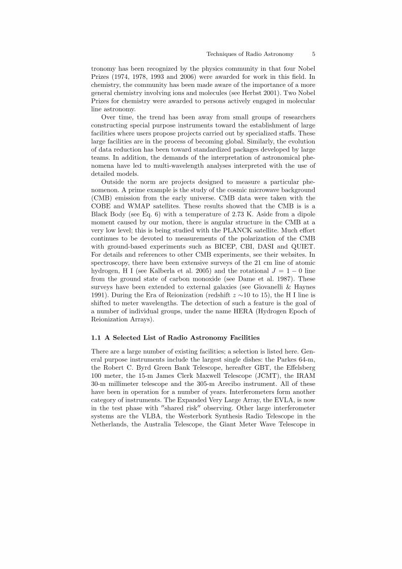
tronomy has been recognized by the physics community in that four NobelPrizes (1974, 1978, 1993 and 2006) were awarded for work in this field. Inchemistry, the community has been made aware of the importance of a moregeneral chemistry involving ions and molecules (see Herbst 2001). Two NobelPrizes for chemistry were awarded to persons actively engaged in molecularline astronomy.

Over time, the trend has been away from small groups of researchersconstructing special purpose instruments toward the establishment of largefacilities where users propose projects carried out by specialized staffs. Theselarge facilities are in the process of becoming global. Similarly, the evolutionof data reduction has been toward standardized packages developed by largeteams. In addition, the demands of the interpretation of astronomical phe-nomena have led to multi-wavelength analyses interpreted with the use ofdetailed models.

Outside the norm are projects designed to measure a particular phe-nomenon. A prime example is the study of the cosmic microwave background(CMB) emission from the early universe. CMB data were taken with theCOBE and WMAP satellites. These results showed that the CMB is is aBlack Body (see Eq. 6) with a temperature of 2.73 K. Aside from a dipolemoment caused by our motion, there is angular structure in the CMB at avery low level; this is being studied with the PLANCK satellite. Much effortcontinues to be devoted to measurements of the polarization of the CMBwith ground-based experiments such as BICEP, CBI, DASI and QUIET.For details and references to other CMB experiments, see their websites. Inspectroscopy, there have been extensive surveys of the 21 cm line of atomichydrogen, H I (see Kalberla et al. 2005) and the rotational J = 1 − 0 linefrom the ground state of carbon monoxide (see Dame et al. 1987). Thesesurveys have been extended to external galaxies (see Giovanelli & Haynes1991). During the Era of Reionization (redshift z ∼10 to 15), the H I line isshifted to meter wavelengths. The detection of such a feature is the goal ofa number of individual groups, under the name HERA (Hydrogen Epoch ofReionization Arrays).

1.1 A Selected List of Radio Astronomy Facilities

There are a large number of existing facilities; a selection is listed here. Gen-eral purpose instruments include the largest single dishes: the Parkes 64-m,the Robert C. Byrd Green Bank Telescope, hereafter GBT, the Effelsberg100 meter, the 15-m James Clerk Maxwell Telescope (JCMT), the IRAM30-m millimeter telescope and the 305-m Arecibo instrument. All of thesehave been in operation for a number of years. Interferometers form anothercategory of instruments. The Expanded Very Large Array, the EVLA, is nowin the test phase with ′′shared risk′′ observing. Other large interferometersystems are the VLBA, the Westerbork Synthesis Radio Telescope in theNetherlands, the Australia Telescope, the Giant Meter Wave Telescope in

6 T. L. Wilson

India, the MERLIN array a number of arrays at Cambridge University inthe UK and the MOST facility in Australia. In the mm range, CARMA inCalifornia and Plateau de Bure in France are in full operation, as is the Sub-Millimeter Array of the Harvard-Smithsonian CfA and ASIAA on MaunaKea, Hawaii. At longer wavelengths, the Low Frequency Array, LOFAR, hasstarted the first measurements and will expand by adding stations throughoutEurope. The Square Kilometer Array, the SKA, is in the planning phase as isthe FASR solar facility, while the Australian SKA Precursor (ASKAP), theSouth African SKA precuror, (MeerKAT), the Murchison Widefield Arrayin Western Australia and Long Wavelength Array in New Mexico are underconstruction. A portion of the Allen Telescope Array, ATA, is in operation.A number of facilities are under construction, being commissioned or haverecently become operational. At sub-mm wavelengths, the Herschel SatelliteObservatory has been delivering data. The Five Hundred Meter ApertureSpherical Telescope, FAST, a design based on the Arecibo instrument, isbeing planned in China. This will be the world’s largest single aperture.The Large Millimeter Telescope, LMT, a joint Mexican-US project, will soonbegin science operations as will the Stratospheric Far-Infrared Observatory(SOFIA) operated by NASA and the German DLR organization. Descrip-tions of these instruments are to be found in the internet. Finally, the mostambitious ground based astronomy project to date is ALMA which will startearly science operations in late 2011 (for an account of the variety of ALMAscience goals, see Bachiller & Cernicharo 2008).

2 Radiative Transfer and Black Body Radiation

The total flux of a source is obtained by integrating Intensity (in Watts m−2

Hz−1 steradian−1) over the total solid angle Ωs subtended by the source

Sν =∫Ωs

Iν(θ, ϕ) cos θ dΩ. (1)

The flux density of astronomical sources is given in units of the Jansky (here-after Jy), that is, 1 Jy = 10−26 W m−2Hz−1.

The equation of transfer is useful in interpreting the behavior of astronom-cial sources, receiver systems, the effect of the earth’s atmosphere on mea-surements. Much of this analysis is based on a one dimensional version of thegeneral expression as (see Lequeux 2004 or Tielens 2005):

dIνds

= −κνIν + εν . (2)

The linear absorption coefficient κν and the emissivity εν are independent ofthe intensity Iν . From the optical depth definition dτν = −κν ds, the Kirch-


hoff relation εν/κν = Bν (see (Eq. 6)) and the assumption of an isothermalmedium, the result is:

Iν(s) = Iν(0) e−τν(s) +Bν(T ) (1− e−τν(s)) . (3)

For a large optical depth, that is for τν(0)→∞, (Eq. 3) approaches the limit

Iν = Bν(T ) . (4)

This is case for planets and the 2.73 K CMB. From (Eq, 3), the differencebetween Iν(s) and Iν(0) gives

∆Iν(s) = Iν(s)− Iν(0) = (Bν(T )− Iν(0))(1− e−τ ) . (5)

this represents the result of an on-source minus off-source measurement,which is relevant for discrete sources.

The spectral distribution of the radiation of a black body in thermody-namic equilibrium is given by the Planck law

Bν(T ) =2hν3

c21

ehν/kT − 1. (6)

If hν kT , the Rayleigh-Jeans Law is obtained:

BRJ(ν, T ) =2ν2

c2kT . (7)

In the Rayleigh-Jeans relation, the brightness and the thermodynamictemperatures of Black Body emitters are strictly proportional (Eq. 7). Thisfeature is useful, so the normal expression of brightness of an extended sourceis brightness temperature TB:

TB =c2

2k1ν2Iν =

λ2

2kIν . (8)

If Iν is emitted by a black body and hν kT then (Eq. 8) gives thethermodynamic temperature of the source, a value that is independent of ν.If other processes are responsible for the emission of the radiation (e.g., syn-chrotron, free-free or broadband dust emission), TB will depend on the fre-quency; however (Eq. 8) is still used. If the condition ν(GHz) 20.84 (T(K))is not valid, (Eq. 8) can still be applied, but TB will differ from the thermo-dynamic temperature of a black body. However, corrections are simple toobtain.

If (Eq. 8) is combined with (Eq. 5), the result is an expression for bright-ness temperature:

J(T ) =c2

2kν2(Bν(T )− Iν(0))(1− e−τν(s)) .

8 T. L. Wilson

The expression J(T ) can be expressed as a temperature in most cases. Thisquantity is referred to as T ∗R, the radiation temperature in the mm/sub-mm range, or the brightness temperature, TB for longer wavelengths. In theRayleigh-Jeans approximation the equation of transfer is:

dTB(s)dτν

= Tbk(0)− T (s) , (9)

where TB is the measured quantity, Tbk(s) is the background source temper-ature and T (s) is the temperature of the intervening medium If the mediumis isothermal, the general (one dimensional) solution becomes

TB = Tbk(0) e−τν(s) + T (1− e−τν(s)) . (10)

2.1 The Nyquist Theorem and Noise Temperature

This theorem relates the thermodynamic quantity temperature to the elec-trical quantities voltage and power. This is essential for the analysis of noisein receiver systems. The average power per unit bandwidth, Pν (also referredto as Power Spectral Density, PSD), produced by a resistor R is

Pν = 〈iv〉 =〈v2〉2R

=1

4R〈v2

N〉 , (11)

where v(t) is the voltage that is produced by i across R, and 〈· · ·〉 indicates atime average. The first factor 1

2 arises from the condition for the transfer ofmaximum power from R over a broad range of frequencies. The second factor12 arises from the time average of v2. Then

〈v2N〉 = 4Rk T . (12)

When inserted into (Eq. 11), the result is

Pν = k T . (13)

(Eq. 13) can also be obtained by a reformulation of the Planck law for onedimension in the Rayleigh-Jeans limit. Thus, the available noise power of aresistor is proportional to its temperature, the noise temperature TN, inde-pendent of the value of R and of frequency.

Not all circuit elements can be characterized by thermal noise. For ex-ample a microwave oscillator can deliver 1 µW, the equivalent of more than1016 K, although the physical temperature is ∼300 K. This is an example of avery nonthermal process, so temperature is not a useful concept in this case.


2.2 Overview of Intensity, Flux Density and Main BeamBrightness Temperature

Temperatures in radio astronomy have given rise to some confusion. A shortsummary with references to later sections is given here. Power is measuredby an instrument consisting of an antenna and receiver. The power input canbe calibrated and expressed as Flux Density or Intensity. For very extendedsources, Intensity (see (Eq. 8)) can be expressed as a temperature, the mainbeam brightness temperature, TMB. To obtain TMB, the measurements mustbe calibrated (Section 5.3) and corrected using the appropriate efficiencies(see Eq. 37 and following). For discrete sources, the combination of (Eq. 1)with (Eq. 8) gives:

Sν =2 k ν2

c2TB ∆Ω . (14)

For a source with a Gaussian spatial distribution, this relation is[SνJy

]= 0.0736TB

[θ

arc seconds

]2 [λ

mm

]−2

(15)

if the flux density Sν and the actual (or ′′true′′) source size are known, thenthe true brightness temperature, TB, of the source can be determined. ForLocal Thermodynamic Equilibrium (LTE), TB represents the physical tem-perature of the source. If the apparent source size, that is, the source angularsize as measured with an antenna is known, (Eq. 15) allows a calculation ofTMB. For discrete sources, TMB depends on the angular resolution. If theantenna beam size (see Fig. 3 and discussion) has a Gaussian shape θb, therelation of actual θs and apparent size θo is:

θ2o = θ2

s + θ2b . (16)

then from (Eq. 14), the relation of TMB and TB is:

TMB

(θ2

s + θ2b

)= TB θ

2s (17)

Finally, the PSD entering the receiver (Eq. 13) is antenna temperature, TA;this is relevant for estimating signal to noise ratios (see (Eq. 39) and (Eq. 42)).To establish temperature scales and relate received power to source param-eters for filled apertures, see Section 5.3. For interferometry and ApertureSynthesis, see Section 6.

2.3 Interstellar Dispersion and Polarization

Pulsars emit radiation in a short time interval (see Lorimer & Kramer 2004,Lyne & Graham-Smith 2006). If all frequencies are emitted at the same in-stant, the arrival time delay of different frequencies is caused by the ionized

10 T. L. Wilson

Interstellar Medium (ISM). This is characterized by the quantity∫ L

0N(l) dl,

which is the column density of the electrons to a distance L. Since distancesin astronomy are measured in parsecs it has become customary to expressthe dispersion measure as:

DM =

L∫0

(N

cm−3

)d(l

pc

)(18)

The lower frequencies are delayed more in the ISM, so the relative time delayis:

∆τDµs

= 1.34× 10−9

[DM

cm−2

] 1( ν1

MHz

)2 −1( ν2

MHz

)2

(19)

Since both time delay ∆τD and observing frequencies ν1 < ν2 can be mea-sured with high precision, a very accurate value of DM for a given pulsarcan be determined. Provided the distance to the pulsar, L, is known, a goodestimate of the average electron density between observer and pulsar canbe found. However since L is usually known with moderate accuracy, onlyapproximate values for N can be obtained. Often the opposite procedure isused: From reasonable values for N , a measured DM provides information onthe unknown distance L to the pulsar.

Broadband linear polarization is caused by non-thermal processes (see Ry-bicki & Lightman 1979) including Pulsar radiation, quasi-thermal emissionfrom aligned, non-spherical dust grains (see Hildebrand 1983) and scatteringfrom free electrons. Faraday rotation will change the position angle of linearpolarization as the radiation passes through an ionized medium; this variesas λ2, so this effect is larger for longer wavelengths. It is usual to characterizepolarization by the four Stokes Parameters, which are the sum or difference ofmeasured quantities. The total intensity of a wave is given by the parameterI. The amount and angle of linear polarization by the parameters Q and U ,while the amount and sense of circular polarization is given by the parame-ter V . Hertz dipoles are sensitive to a single linear polarization. By rotatingthe dipole over an angle perpendicular to the direction of the radiation, it ispossible to determine the amount and angle of linearly polarized radiation.Helical antennas or arrangements of two Hertz dipoles are sensitive to circu-lar polarization. Generally, polarized radiation is a combination of linear andcircular, and is usually less than 100% polarized, so four Stokes parametersmust be specified. The definition of the sense of circular polarization in ra-dio astronomy is the same as in Electrical Engineering but opposite to thatused in the optical range; see Born & Wolf (1965) for a complete analysisof polarization, using the optical definition of circular polarization. Poincareintroduced a representation that permits an easy visualization of all the dif-ferent states of polarization of a vector wave. See Thompson et al. (2001),Crutcher (2008), Thum et al. (2008) or Wilson et al. (2008) for more details.


3 Receiver Systems

3.1 Coherent and Incoherent Receivers

Receivers are assumed to be linear power measuring devices, i. e. anynon-linearity is a small quantity. There are two types of receivers: coher-ent and incoherent. Coherent receivers are those which preserve the phaseof the input radiation while incoherent do not. Heterodyne (technically′′superheterodyne′′) receivers are those which those which shift the frequencyof the input but preserve phase. The most commonly used coherent receiversemploy heterodyning, that is, frequency shifting (see Section 4.2.1). The mostcommonly used incoherent receivers are bolometers (Section 4.1); these aredirect detection receivers, that is, operate at sky frequency. Both coherent andincoherent receivers add noise to the astronomical input signal; it is assumedthat the noise of both the input signal and the receiver follow Gaussian distri-butions. The noise contribution of coherent receivers is expressed in Kelvins.Bolometer noise is characterized by the Noise Equivalent Power, or NEP, inunits of Watts Hz−1/2 (see Section 3.1.1 and Section 5.3.3). NEP is the inputpower level which doubles the output power. More extensive discussions ofreceiver properties are given in Rieke (2002) or Wilson et al. (2008).

To analyze the performance of a receiver, the commonly accepted modelis an ideal receiver with no internal noise, but connected to two noise sources,one for the external noise (including the astronomical signal) and a secondfor the receiver noise. To be useful, receiver systems must increase the inputpower level. The noise contribution is characterized by the Noise Factor, F .If the signal-to-noise ratio at the input is expressed as (S1/N1) and at theoutput as (S2/N2), the noise factor is:

F =S1/N1

S2/N2. (20)

A further step is to assume that the signal is amplified by a gain factor Gbut otherwise unchanged. Then S2 = GS1 and:

F =N2

GN1. (21)

For a direct detection system such as a bolometer, G = 1. For coherentreceivers, there must be a minimum noise contribution (see Section 4.2.4),so F > 1. For coherent receivers F is expressed in temperature units as TRusing the relation

TR = (F − 1) · 290K . (22)

3.1.1 Receiver Calibration

Heterodyne receiver noise performance is usually expressed in degrees Kelvin.In the calibration process, a power scale (the PSD) is established at the re-ceiver input. This is measured in terms of the noise temperature. To calibrate

12 T. L. Wilson

a receiver, the noise temperature increment ∆T at the receiver input mustbe related to a given measured receiver output increment ∆z (this appliesto coherent receivers which have a wide dynamic range and a total poweror ′′DC′′ response). Usually resistive loads at two known (thermodynamic)temperatures TL and TH are used. The receiver outputs are zL and zH, whileTL and TH are the resistive loads at two temperatures. The relations are:

zL = (TL + TR)G ,zH = (TH + TR)G ,

takingy = zH/zL . (23)

the result is:

Trx =TH − TL y

y − 1, (24)

This is known as the ′′y-factor′′; the procedure is a ′′hot-cold′′ measurement.The determination of the y factor is calculated in the Rayleigh-Jeans limit.Absorbers at temperatures of TH and TL are used to produce the inputs. Oftenthese are chosen to be at the ambient temperature (TH

∼= 293 K or 20C)and at the temperature of liquid nitrogen (TL

∼= 78 K or −195 C). Whenreceivers are installed on antennas, such ′′hot-cold′′ calibrations are doneonly infrequently. As will be discussed in Section 5.3.2, in the cm and meterrange, calibration signals are provided by noise diodes; from measurementsof sources with known flux densities intensity scales are established. Anyatmospheric corrections are assumed to be small at these wavelengths. Aswill be discussed in Section 5.3.3, in the mm/sub-mm wavelength range, frommeasurements of an ambient load (or two loads at different temperatures),combined with measurements of emission from the atmosphere and modelsof the atmosphere, estimates of atmospheric transmission are made.

Bolometer performance is characterized by the Noise Equivalent Power,or NEP, given in units of Watts Hz−1/2. The expression for NEP can berelated to a receiver noise temperature. For ground based bolometer systems,background noise dominates. For these, the background noise is given as TBG:

NEP = 2ε k TBG

√∆ν . (25)

here ε is the emissivity of the background and ∆ν is the bandwidth. Typicalvalues for ground-based mm/sub-mm bolometers are ε = 0.5, TBG = 300K and ∆ν = 100 GHz. For these values, NEP= 1.3 × 10−15 Watts Hz−1/2.With the collecting area of the IRAM 30 m or the JCMT telescopes, sourcesin the milli-Jansky (mJy) range can be measured.

Usually bolometers are ′′A. C.′′ coupled, that is, the output responds todifferences in the input power, so hot-cold measurements are not useful for


characterizing bolometers. The response of bolometers is usually determinedby measurements of sources with known flux densities, followed by measure-ments at, for example, elevations of 20o, 30o, 60o and 90o to determine theatmospheric transmission (see Section 5.3.4).

3.1.2 Noise Uncertainties due to Random Processes

The noise contributions from source, atmosphere, ground, telescope surfaceand receiver are always additive:

Tsys =∑

Ti (26)

From Gaussian statistics, the Root Mean Square, RMS, noise is given bythe mean value divided by the square root of the number of samples. Fromthe estimate that the number of samples is given by the product of receiverbandwidth multiplied by the integration time, the result is:

∆TRMS =Tsys√∆ν τ

. (27)

A much more elaborate derivation is to be found in Chapter 4 of Rohlfs &Wilson (2004), while a somewhat simpler account is in Wilson et al. (2008).The calibration process in (Section 3.1.1) allows the receiver noise to beexpressed in degrees Kelvin. The relation of Tsys to Trx is Tsys = TA + Trx,where TA represents the power entering the receiver; at some wavelengths TA

will dominate Trx. In the mm/sub-mm range, use is made of T∗sys, the systemnoise outside the atmosphere, since the attenuation of astronomical radiationis large. This will be presented in Section 5.3.1 and following.

3.1.3 Receiver Stability

Sensitive receivers are designed to achieve a low value for Trx. Since the sig-nals received are of exceedingly low power, receivers must also provide largereceiver gains, G (of order 1012), for sufficient output power. Thus even verysmall gain instabilities can dominate the thermal receiver noise. Since receiverstability considerations are of prime importance, comparison switching wasnecessary for early receivers (Dicke 1946). Great advances have been made inimproving receiver stability since the 1960’s so the need for rapid switching islessened. In the meter and cm wavelength range, the time between referencemeasurements has increased. However in the mm/sub-mm range, instabilitiesof the atmosphere play an important role; to insure that noise decreases fol-lowing (Eq. 27), the effects of atmospheric and/or receiver instabilities mustbe eliminated. For single dish measurements, atmospheric changes can becompensated for by rapidly differencing a measurement of the target source

14 T. L. Wilson

and a reference. Such comparison or ′′Dicke′′ switched measurements are nec-essary for ground-based observations. If a typical procedure consists of usinga total power receiver to measure on-source for 1/2 of the total time, thenan off-source comparison for 1/2 of the time and taking the difference of on-source minus off-source measurements, the ∆TRMS will be a factor of 2 largerthan the value given by (Eq. 27).

4 Practical Aspects of Receivers

This section concentrates on receivers that are currently in use. For moredetails see Goldsmith (1988), Rieke (2002), or Wilson et al. (2008).

4.1 Bolometer Radiometers

Bolometers operate by use of the effect that the resistance, R, of a materialvaries with the temperature. In the 1970’s, the most sensitive bolometerswere semiconductor devices pioneered by F. Low. This is achieved when thebolometer element is cooled to very low temperatures. When radiation is in-cident, the characteristics change, so this is a measure of the intensity of theincident radiation. Because this is a thermal effect, it is independent of thefrequency and polarization of the radiation absorbed. Thus bolometers are in-trinsically broadband devices. It is possible to mount a polarization-sensitivedevice before the bolometer and thereby measure the direction and degree oflinear polarization. Also, it is possible to carry out spectroscopy, if frequencysensitive elements, either filters, Michelson or Fabry-Perot interferometers,are placed before the bolometer element. Since these spectrometers operateat the sky frequency, the fractional resolution (∆ν/ν) is at best ∼ 10−4. Thedata from each bolometer detector element (pixel) must be read out and thenamplified.

For single dish (i. e. filled apertures) broadband continuum measurementsat λ < 2 mm, multi-beam bolometers are the most common systems and suchsystems can have a large number of beams. A promising new development inbolometer receivers is Transition Edge Sensors referred to as TES bolometers.These superconducting devices may allow more than an order of magnitudeincrease in sensitivity, if the bolometer is not background limited. For bolome-ters used on earth-bound telescopes, the improvement with TES systems maybe only ∼2–3 times more sensitive than the semiconductor bolometers, butTES’s will allow readouts from a much larger number of pixels.

A number of large bolometer arrays have produced numerous publications:(1) MAMBO2 (MAx-Planck-Millimeter Bolometer) used on the IRAM 30-mtelescope at 1.3 mm, (2) SCUBA (Submillimeter Common User Bolome-ter Array; Holland et al. 1999) on the JCMT, (3) the LABOCA (LArgeBolometer CAmera) array on the APEX 12 meter telescope, (4) SHARC


(Sub-mm High Angular Resolution Camera) on the Caltech Sub-mm Obser-vatory 10-m telescope and (5) MUSTANG (MUtiplexed Squid TES Array)on the GBT. SCUBA will be replaced with SCUBA-2 now being constructedat the U. K. Astronomy Technology Center, and there are plans to replacethe MUSTANG array by MUSTANG-2, which is a larger TES system.

4.2 Coherent Receivers

Usually, coherent receivers make use of heterodyning to shift the signal inputfrequency without changing other properties of the input signal; in practice,this is carried out by the use of mixers (Section 4.2.2). The heterodyne processis used in all branches of communications technology; use of heterodyning al-lows measurements with unlimited spectral resolution. Although heterodynereceivers have a number of components, these systems have more flexibilitythan bolometers.

4.2.1 Noise Contributions in Coherent Receivers

The noise generated in the first element dominates the system noise. Themathematical expression is given by the Friis relation which accounts for theeffect of cascaded amplifiers on the noise performance of a receiver:

TS = TS1 +1G1

TS2 +1

G1G2TS3 + . . .+

1G1G2 . . . Gn−1

TSn . (28)

Where G1 is the gain of the first element, and TS1 is the noise temperatureof this element. For λ >3 mm (ν < 115GHz), the best cooled first elements,High Electron Mobility Transistors (HEMTs), typically have G1 = 103 andTS1 = 50K; for λ <0.8 mm, the best cooled first elements, superconductingmixers, typically have G1 ≤ 1, that is, a small loss, and TS1 ≤ 500K. Thestage following the mixer should have the lowest noise temperature and highgain.

4.2.2 Mixers

Mixers have been used in heterodyne receivers since Jansky’s time. At firstthese were metal-oxide-semiconductor or Schottky mixers. Mixers allow thesignal frequency to be changed without altering the characteristics of thesignal. In the mixing process, the input signal is multiplied by an intensemonochromatic signal from a local oscillator, LO. The frequency stability ofthe LO signal is maintained by a stabilization device in which the LO signalis compared with a stable input, in recent times, an atomic standard. Thesephaselock loop systems produce a pure, highly stable, monochromatic signal.The mixer can be operated in the Double Sideband (DSB) mode, in which

16 T. L. Wilson

two sky frequencies, ′′signal′′ and ′′image′′ at equal separations from the LOfrequency (equal to the IF frequency) are shifted into intermediate (IF) fre-quency band. For spectral line measurements, usually one sideband is wanted,but the other not. DSB operation adds both noise and (usually) unwantedspectral lines; for spectral line measurements, single sideband (SSB) opera-tion is preferred. In SSB operation, the unwanted sideband is suppressed, atthe cost of more complexity. In the sub-mm wavelength ranges, DSB mixersare still commonly used as the first stage of a receiver; in the mm and cmranges, SSB operation is now the rule.

A significant improvement can be obtained if the mixer junction is oper-ated in the superconducting mode. The noise temperatures and LO powerrequirements of superconducting mixers are much lower than Schottky mix-ers. Finally, the physical layout of such devices is simpler since the mixeris a planar device, deposited on a substrate by lithographic techniques. SISmixers consist of a superconducting layer, a thin insulating layer and anothersuperconducting layer (see Phillips & Woody 1982).

Superconducting Hot Electron Bolometer-mixers (HEB) are heterodynedevices, in spite of the name. These mixers make use of superconducting thinfilms which have sub-micron sizes (see Kawamura et al. 2002).

A number of multi-beam heterodyne cameras are in operation in the cmrange, but only a few in the mm/sub-mm range. The first mm multi-beamsystem was the SEQUOIA array receiver pioneered by S. Weinreb; such de-vices are becoming more common. In contrast, multibeam systems that useSIS front ends are rare. Examples are a 9 beam Heterodyne Receiver Arrayof SIS mixers at 1.3 mm, HERA, on the IRAM 30-m millimeter telescope,HARP-B, a 16 beam SIS system in operation at the JCMT for 0.8 mm andthe CHAMP+ receiver at the Max-Planck-Inst. fur Radioastronomy on theAPEX 12-m telescope.

4.2.3 Square Law Detectors

For heterodyne receivers the input is normally amplified (for ν < 115GHz),translated in frequency and then detected in a device that produces an outputsignal y(t) which is proportional to the square of v(t):

y(t) = a v2(t) (29)

Once detected, phase information is lost. For interferometers, the output ofeach antenna is a voltage, shifted in frequency and then digitized. This outputis brought to a central location for correlation.

4.2.4 The Minimum Noise in a Coherent System

The ultimate limit for coherent receivers or amplifiers is obtained by an ap-plication of the Heisenberg uncertainty principle involving phase and number


Fig. 2. Receiver noise temperatures for coherent amplifier systems compared tothe temperatures from the Milky Way galaxy (at long wavelengths, on left part offigure) and the atmosphere (at mm/sub-mm wavelengths on the right side). Theatmospheric emission is based on a model of zenith emission for 0.4 mm of watervapor, that is, excellent weather (plot from B. Nicolic (Cambridge Univ.) usingthe ′′AM′′ program of S. Paine (Harvard-Smithsonian Center for Astrophysics)).This does not take into account the absorption of the astronomical signal. In the1 to 26 GHz range, the two horizontal lines represent the noise temperatures ofthe best HEMT amplifiers, while the solid line represents the noise temperaturesof maser receivers. The shaded region between 85 and 115.6 GHz is the receivernoise for the SEQUOIA array (Five College Radio Astronomy Observatory) whichconsists of monolithic millimeter integrated circuits (MMIC). The meaning of theother symbols is given in the upper left of the diagram (SIS’s are Superconductor-Insulator-Superconductor mixers, HEB’s are Hot Electron Bolometer mixers). Thedouble sideband (DSB) mixer noise temperatures were converted to single sideband(SSB) noise temperatures by doubling the receiver noise. The ALMA mixer noisetemperatures are SSB, as are the HEMT values. The line marked ′′10 hν/kT′′ refersto the limit described in (Eq. 30). Some data used in this diagram are taken fromRieke (2002). The figure is from Wilson et al. (2008)

18 T. L. Wilson

of photons. From this, the minimum noise of a coherent amplifier results ina receiver noise temperature of

Trx(minimum) =hν

k. (30)

For incoherent detectors, such as bolometers, phase is not preserved, so thislimit does not exist. In the mm wavelength region, this noise temperaturelimit is quite small; at λ=2.6 mm (ν=115 GHz), this limit is 5.5 K. The valuefor the ALMA receiver in this range is about 5 to 6 times the minimum. Asignificant difference between radio and optical regimes is that the minimumnoise in the radio range is small, so that the power from a single receivercan be amplified and then divided. For example, for the EVLA, the voltageoutput of all 351 antenna pairs are combined with little or no loss in thesignal-to-noise ratio. Another example is given in Section 4.3.1, where a radiopolarimeter can produce all four Stokes parameters from two inputs withouta loss of the signal-to-noise ratio.

4.3 Back Ends: Polarimeters & Spectrometers

The term ′′Back End′′ is used to specify the devices following the IF ampli-fiers. Many different back ends have been designed for specialized purposessuch as continuum, spectral or polarization measurements.

For a single dish continuum correlation receiver, the (identical) receiverinput is divided, amplified in two identical systems and then the outputs aremultiplied. The gain fluctuations are uncorrelated but the signals are, so theeffect on the output is the same as with a Dicke switched system, but withno time spent on a reference.

4.3.1 Polarimeters

A typical heterodyne dual polarization receiver consists of two identical sys-tems, each sensitive to one of the two orthogonal polarizations, linear orcircular. Both systems must be connected to the same local oscillator toinsure that the phases have a definite relation. Given this arrangement, apolarimeter can provide values of all four Stokes parameters simultaneously.All Stokes parameters can also be measured using a single receiver whoseinput is switched from one sense of polarization to the other, but then theintegration time for each polarization will be halved.

4.3.2 Spectrometers

Spectrometers analyze the spectral information contained in the radiationfield. To accomplish this, the spectrometer must be SSB and the frequency


resolution ∆ν is usually very good, sometimes in the kHz range. In addition,the time stability must be high. If a resolution of ∆ν is to be achieved forthe spectrometer, all those parts of the system that enter critically into thefrequency response have to be maintained to better than 0.1∆ν. For anoverview of the current state of spectrometers, see Baker et al. (2007).

Conceptually, the simplest spectrometer is composed of a set of n adja-cent filters, each with a bandwidth ∆ν. Following each filter is a square-lawdetector and integrator. For a finer resolution, another set of n filters mustbe constructed.

Another approach to spectral analysis is to Fourier Transform (FT) theinput, v(t), to obtain v(ν) and then square v(ν) to obtain the Power SpectralDensity. The maximum bandwidth is limited by the sampling rate. From(another!) Nyquist theorem, it is necessary to sample at a rate equal to twicethe bandwidth. In the simplest scheme, for a bandwidth of 1 GHz, the sam-pling must occur at a rate of 2 GHz. After sampling and Fourier Transform,the output is squared to produce power in an ′′FX′′ autocorrelator. For 103

samples, each channel will have a 1 MHz resolution.For ′′XF′′ systems, the input v(t) is multiplied (the ′′X′′) with a delayed

signal v(t − τ) to obtain the autocorrelation function R(τ). This is thenFourier Transformed to obtain the spectrum. For 103 samples, there will be103 frequency channels. For an XF system the time delays are performedin a set of serial digital shift registers with a sample delayed by a time τ .Autocorrelation can also be carried out with the help of analog devices usinga series of cable delay lines; these can provide very large bandwidths. The firstXF system for astronomy was a digital autocorrelator built by S. Weinreb in1963.

The two significant advantages of digital spectrometers are: (1) flexibilityand (2) a noise behavior that follows 1/

√t after many hours of integration.

The flexibility allows the choice of many different frequency resolutions andbandwidths or even to employ a number of different spectrometers, each withdifferent bandwidths, simultaneously.

A serious drawback of digital auto and cross correlation spectrometershad been limited bandwidths. However, advances in digital technology inrecent years have allowed the construction of autocorrelation spectrometerswith several 103 channels covering instantaneous bandwidths of several GHz.

Autocorrelation systems are used in single antennas. The calculation ofspectra makes use of the symmetric nature of the autocorrelation function,ACF, so the number of delays gives the number of spectral channels.

Cross-correlators are used in interferometers and in some single dish ap-plications. When used in an interferometer, the cross-correlation is betweendifferent inputs so will not necessarily be symmetric. Thus, the zero delayof the cross-correlator is placed in channel N/2. The number of delays, N ,allows the determination of N/2 spectral intensities, and N/2 phases. The

20 T. L. Wilson

cross-correlation hardware can employ either an XF or a FX correlator. Formore details about the use of cross-correlation, see Section 6.

Until recently, spectrometers with bandwidths of several GHz often madeuse of Acoustic Optical analog techniques. The Acoustic Optical Spectrom-eter (AOS) makes use of the diffraction of light by ultrasonic waves: thesecause periodic density variations in the crystal through which it passes. Thesedensity variations in turn cause variations in the bulk constants of the crystal,so that a plane light wave passing through this medium will be modulated bythe interaction with the crystal. The modulated light is detected in a chargecoupled device. Typical AOS’s have an instantaneous bandwidth of 2 GHzand 2000 spectral channels.

In all cases, the spectra of the individual channels of a spectrometer areexpressed in terms of temperature with the relation:

Ti = [(Si −Ri) /Ri] · Tsys (31)

where Si is the normalized spectrum of channel i for the on-source measure-ment and Ri is the corresponding reference for this channel. For mm/sub-mmspectra, Tsys is replaced by T ∗sys (corrected for atmospheric losses; see Section5.3.3). For cross-correlators, as used in interferometers, the signals from twoantennas are multiplied. In this case, the value of Tsys is the square root ofthe product of the system noise temperatures of the two systems.

5 Antennas

The antenna serves to focus power into the feed, a device that efficientlytransfers power in the electromagnetic wave to the receiver. According to theprinciple of reciprocity, the properties of antennas such as beam sizes, efficien-cies etc. are the same whether these are used for receiving or transmitting.Reciprocity holds in astronomy, so it is usual to interchangeably use expres-sions that involve either transmission or reception when discussing antennaproperties. All of the following applies to the far-field radiation.

5.1 The Hertz Dipole

The total power radiated from a Hertz dipole carrying an oscillating currentI at a wavelength λ is

P =2c3

(I∆l

2λ

)2

. (32)

For the Hertz dipole, the radiation is linearly polarized with the electricfield along the direction of the dipole. The radiation pattern has a donutshape, with the cylindrically symmetric maximum perpendicular to the axis


of the dipole. Along the direction of the dipole, the radiation field is zero.To improve directivity, reflecting screens have been placed behind a dipole,and in addition, collections of dipoles, driven in phase, are used. Hertz dipoleradiators have the best efficiency when the size of the dipole is 1/2λ .

5.2 Filled Apertures

This Section is a simplified description of antenna properties needed forthe interpretation of astronomical measurements. For more detail, see Baars(2007). At cm and shorter wavelengths, flared waveguides (′′feed horns′′) ordipoles are used to convey power focussed by the antenna (i. e., electromag-netic waves in free space) to the receiver (voltage). At the longest wavelengths,dipoles are used as the antennas. Details are to be found in Love (1976) andGoldsmith (1988, 1994).

5.2.1 Angular Resolution and Efficiencies

From diffraction theory (see Jenkins & White 2001), the angular resolutionof a reflector of diameter D at a wavelength λ is

θ = kλ

D. (33)

where k is of order unity. This universal result gives a value for θ (here inradians when D and λ have the same units). Diffraction theory also predictsthe unavoidable presence of sidelobes, i. e. secondary maxima. The sidelobescan be reduced by tapering the antenna illumination. Tapering lowers theresponse to very compact sources and increases the value of θ, i. e. widensthe beam.

The reciprocity concept provides a method to measure the power pattern(response pattern or Point Spread Function, PSF) using transmitters. How-ever, the distance from a large antenna A (diameter D λ) to a transmitterB (small in size) must be so large that B produces plane waves across theaperture D of antenna A, that is, so B is in the far field of A. This is theRayleigh distance; it requires that the curvature of a wavefront emitted byB is much less than λ/16 across the geometric dimensions of antenna A. Bydefinition, at the Rayleigh distance D, the curvature must be D2/8λ foran antenna of diameter D.

Often, the normalized power pattern is measured:

Pn(ϑ, ϕ) =1

PmaxP (ϑ, ϕ) . (34)

For larger apertures, the transmitter is usually replaced by a small diameterradio source of known flux density (see Baars et al. 1977, Ott et al. 1994).

22 T. L. Wilson

The flux densities of a few primary calibration sources are determined bymeasurements using horn antennas at centimeter and millimeter wavelengths.At mm/sub-mm wavelengths, it is usual to employ planets, or moons ofplanets, whose surface temperatures are known (see Altenhoff 1985, Sandell1994).

Fig. 3. A polar power pattern showing the main beam, andnear and far sidelobes. The weaker far sidelobes have beencombined to form the stray pattern

The beam solid angle ΩA of an antenna is given by

ΩA =∫ ∫4π

Pn(ϑ, ϕ) dΩ =

2π∫0

π∫0

Pn(ϑ, ϕ) sinϑ dϑdϕ (35)

this is measured in steradians (sr). The integration is extended over all angles,so ΩA is the solid angle of an ideal antenna having Pn = 1 for ΩA and Pn = 0everywhere else. For most antennas the (normalized) power pattern has muchlarger values for a limited range of both ϑ and ϕ than for the remainder; therange where ΩA is large is the main beam of the antenna; the remainder arethe sidelobes or backlobes (Fig. 3).

In analogy to (Eq. 35) the main beam solid angle ΩMB is defined as

ΩMB =∫ ∫mainlobe

Pn(ϑ, ϕ) dΩ . (36)

The quality of a single antenna depends on how well the power pattern isconcentrated in the main beam. The definition of main beam efficiency orbeam efficiency, ηB, is:


ηB =ΩMB

ΩA. (37)

ηB is the fraction of the power is concentrated in the main beam. The mainbeam efficiency can be modified (within limits) for parabolic antennas bychanging the illumination of the main reflector. An underilluminated antennahas a wider main beam but lower sidelobes. The angular extent of the mainbeam is usually described by the full width to half power width (FWHP), theangle between points of the main beam where the normalized power patternfalls to 1/2 of the maximum. For elliptically shaped main beams, values forwidths in orthogonal directions are needed. The beamwidth, θ is given by(Eq. 33). If the FWHP beamwidth is well defined, the location of an isolatedsource is determined to the accuracy given by the FWHP divided by theS/N ratio. Thus, it is possible to determine positions to small fractions of theFWHP beamwidth, if the signal-to-noise ratio is high and noise is the onlylimit.

If a plane wave with the power density | 〈S〉 | in Watts m−2 is interceptedby an antenna, a certain amount of power is extracted from this wave. Thispower is Pe and the fraction is:

Ae = Pe / | 〈S〉 | (38)

the effective aperture of the antenna. Ae has the dimension of m2. Comparedto the geometric aperture Ag an aperture efficiency ηA can be defined by:

Ae = ηAAg . (39)

If an antenna with a normalized power pattern Pn(ϑ, ϕ) is used to receiveradiation from a brightness distribution Bν(ϑ, ϕ) in the sky, at the outputterminals of the antenna the power per unit bandwidth (PSD), in WattsHz−1, Pν is:

Pν = 12 Ae

∫ ∫Bν(ϑ, ϕ)Pn(ϑ, ϕ) dΩ . (40)

By definition, this operates in the Rayleigh-Jeans limit, so the equivalent dis-tribution of brightness temperature can be replaced by an equivalent antennatemperature TA (Eq. 13):

Pν = k TA . (41)

This definition of antenna temperature relates the output of the antenna tothe power from a matched resistor. When these two power levels are equal,then the antenna temperature is given by the temperature of the resistor. Theeffective aperture Ae can be replaced by the the beam solid angle ΩA · λ2.Then (Eq. 40) becomes

24 T. L. Wilson

TA(ϑ0, ϕ0) =∫TB(ϑ, ϕ)Pn(ϑ− ϑ0, ϕ− ϕ0) sinϑ dϑ dϕ∫

Pn(ϑ, ϕ) dΩ(42)

From (Eq. 42), TA < TB in all cases. The numerator is the convolution ofthe brightness temperature with the beam pattern of the telescope (Fouriermethods are of great value in this analysis; see Bracewell 1986). The bright-ness temperature Tb(ϑ, ϕ) corresponds to the thermodynamic temperature ofthe radiating material only for thermal radiation in the Rayleigh-Jeans limitfrom an optically thick source; in all other cases TB is a convenient quantitythat represents source intensity at a given frequency. The quantity TA in(Eq. 42) was obtained for an antenna in which ohmic losses and absorptionin the earth’s atmosphere were neglected. These losses can be corrected inthe calibration process. Since TA is the quantity measured while TB is de-sired, (Eq. 42) must be inverted. (Eq. 42) can be solved only if TA(ϑ, ϕ) andPn(ϑ, ϕ) are known exactly over the full range of angles. In practice this in-version is possible only approximately, since both TA(ϑ, ϕ) and Pn(ϑ, ϕ) areknown only for a limited range of ϑ and ϕ values, and the measured dataare affected by noise. Therefore only an approximate deconvolution can beperformed. If the source distribution TB(ϑ, ϕ) has a small extent comparedto the telescope beam, the best estimate for the upper limit to the actualFWHP source size is 1/2 of the FWHP of the telescope beam.

5.2.2 Efficiencies for Compact Sources

For a source small compared to the beam (Eq. 40) and (Eq. 41) give:

Pν = 12Ae Sν = k TA (43)

TA is the antenna temperature at the receiver, while T ′A is this quantitycorrected for effect of the earth’s atmosphere. In the meter and cm rangeTA = T ′A, so in the following, T ′A will be used:

T ′A = ΓSν (44)

where Γ is the sensitivity of the telescope measured in K Jy−1. Introducingthe aperture efficiency ηA according to (Eq. 39) we find

Γ = ηAπD2

8k. (45)

Thus Γ or ηA can be measured with the help of a calibrating source providedthat the diameter D and the noise power scale in the receiving system areknown. When (Eq. 44) is solved for Sν , the result is:


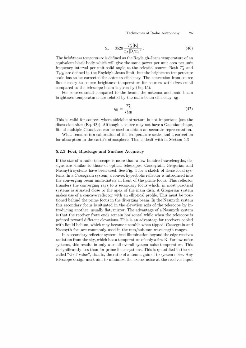
Sν = 3520T ′A[K]

ηA[D/m]2. (46)

The brightness temperature is defined as the Rayleigh-Jeans temperature of anequivalent black body which will give the same power per unit area per unitfrequency interval per unit solid angle as the celestial source. Both T ′A andTMB are defined in the Rayleigh-Jeans limit, but the brightness temperaturescale has to be corrected for antenna efficiency. The conversion from sourceflux density to source brightness temperature for sources with sizes smallcompared to the telescope beam is given by (Eq. 15).

For sources small compared to the beam, the antenna and main beambrightness temperatures are related by the main beam efficiency, ηB:

ηB =T ′ATMB

. (47)

This is valid for sources where sidelobe structure is not important (see thediscussion after (Eq. 42)). Although a source may not have a Gaussian shape,fits of multiple Gaussians can be used to obtain an accurate representation.

What remains is a calibration of the temperature scales and a correctionfor absorption in the earth’s atmosphere. This is dealt with in Section 5.3

5.2.3 Foci, Blockage and Surface Accuracy

If the size of a radio telescope is more than a few hundred wavelengths, de-signs are similar to those of optical telescopes. Cassegrain, Gregorian andNasmyth systems have been used. See Fig. 4 for a sketch of these focal sys-tems. In a Cassegrain system, a convex hyperbolic reflector is introduced intothe converging beam immediately in front of the prime focus. This reflectortransfers the converging rays to a secondary focus which, in most practicalsystems is situated close to the apex of the main dish. A Gregorian systemmakes use of a concave reflector with an elliptical profile. This must be posi-tioned behind the prime focus in the diverging beam. In the Nasmyth systemthis secondary focus is situated in the elevation axis of the telescope by in-troducing another, usually flat, mirror. The advantage of a Nasmyth systemis that the receiver front ends remain horizontal while when the telescope ispointed toward different elevations. This is an advantage for receivers cooledwith liquid helium, which may become unstable when tipped. Cassegrain andNasmyth foci are commonly used in the mm/sub-mm wavelength ranges.

In a secondary reflector system, feed illumination beyond the edge receivesradiation from the sky, which has a temperature of only a few K. For low-noisesystems, this results in only a small overall system noise temperature. Thisis significantly less than for prime focus systems. This is quantified in the so-called ′′G/T value′′, that is, the ratio of antenna gain of to system noise. Anytelescope design must aim to minimize the excess noise at the receiver input

26 T. L. Wilson

Fig. 4. The geometry of parabolic apertures: (a) Cassegrain, (b) Gregorian, (c)Nasmyth and (d) offset Cassegrain systems (from Wilson et al. 2008).

while maximizing gain. For a specific antenna, this maximization involves thedesign of feeds and the choice of foci.

The secondary reflector and its supports block the central parts in themain dish from reflecting the incoming radiation, causing some significantdifferences between the actual beam pattern and that of an unobstructedantenna. Modern designs seek to minimize blockage due to the support legsand subreflector.

The beam pattern differs from a uniformly illuminated unblocked aperturefor 3 reasons:(1) the illumination of the reflector will not be uniform but has a taper by10 dB, that is, a factor of 10 or more at the edge of the reflector. This is incontrast to optical telescopes which have no taper.(2) the side-lobe level is strongly influenced by this taper: a larger taperlowers the sidelobe level.(3) the secondary reflector must be supported by three or four support legs,which will produce aperture blocking and thus affect the shape of the beampattern.

Feed leg blockage will cause deviations from circular symmetry. Foraltitude-azimuth telescopes these sidelobes will change position on the skywith hour angle (see Reich et al. 1978). This may be a serious defect, sincethese effects will be significant for maps of low intensity regions near an in-tense source. The sidelobe response may depend on the polarization of theincoming radiation (see Section 5.3.6).

A disadvantage of on-axis systems, regardless of focus, is that they areoften more susceptible to instrumental frequency baselines, so-called baselineripples across the receiver band than primary focus systems (see Morris 1978).Part of this ripple is caused by reflections of noise from source or receiverin the antenna structure. Ripples from the receiver can be removed if theamplitude and phase are constant in time. Baseline ripples caused by the


source, sky or ground radiation are more difficult to eliminate since these willchange over short times. It is known that large amounts of blockage and largerfeed sizes lead to large baseline ripples. The influence of baseline ripples onmeasurements can be reduced to a limited extent by appropriate observingprocedures. A possible solution is an off-axis system such as the GBT ofthe National Radio Astronomy Observatory. In contrast to the GBT, theEffelsberg 100-m has a large amount of blocking from massive feed supportlegs and, as a result, show large instrumental frequency baseline ripples. Theseripples might be mitigated by the use of scattering cones in the reflector.

The gain of a filled aperture antenna with small scale surface irregularitiesε cannot increase indefinitely with increasing frequency but reaches a maxi-mum at λm = 4πε, and this gain is a factor of 2.7 below that of an error-freeantenna of identical dimensions. The usual rule-of-thumb is that the irregu-larities should be 1/16 of the shortest wavelength used. Larger filled apertureradio telescopes are made up of panels. For these, the irregularities are oftwo types: (1) roughness of the individual panels, and (2) misadjustment ofpanels. The second irregularity gives rise to an error beam. The FWHP ofthe error beam is given approximately by the ratio of wavelength to panelsize. In addition, if the surface material is not a perfect conductor, there willbe some loss and consequently additional noise.

5.3 Single Dish Observational Techniques

5.3.1 The Earth’s Atmosphere

For ground–based facilities, the amplitudes of astronomical signals have beenattenuated and the phases have been altered by the earth’s atmosphere. Inaddition to attenuation, the receiver noise is increased by atmospheric emis-sion, the signal is refracted and there are changes in the path length. Theseeffects may change slowly with time, but there can also be rapid changes suchas scintillation and anomalous refraction. Thus propagation properties mustbe taken into account if the astronomical measurements are to be correctlyinterpreted. At meter wavelengths, these effects are caused by the ionosphere.In the mm/sub-mm range, tropospheric effects are especially important. Thevarious constituents of the atmosphere absorb by different amounts. Becausethe atmosphere can be considered to be in LTE, these constituents also emitradiation.

The total amount of precipitable water (usually measured in mm) is anintegral along the line-of-sight to a source. Frequently, the amount of H2O isdetermined by measurements of the continuum emission of the atmospherewith a small dish at 225 GHz. For a set of measurements at elevations of20o, 30o, 60o and 90o, combined with models, rather accurate values of theatmospheric τ can be obtained. For extremely dry mm/sub-mm sites, mea-surements of the 183 GHz spectral line of water vapor can be used to estimatethe total amount of H2O in the atmosphere. For sea level sites, the 22.235

28 T. L. Wilson

GHz line of water vapor has been used for this purpose. The scale heightHH2O ≈ 2 km, is considerably less than Hair ≈ 8 km of dry air. For this rea-son, sites for submillimeter radio telescopes are usually mountain sites withelevations above ≈ 3000 m. For ionospheric effects, even the highest sites onearth provide no improvement.

The effect on the intensity of a radio source due to propagation throughthe atmosphere is given by the standard relation for radiative transfer (from(Eq. 10)):

TB(s) = TB(0) e−τν(s) + Tatm (1− e−τν(s)) . (48)

Here s is the (geometric) path length along the line-of-sight with s = 0at the upper edge of the atmosphere and s = s0 at the antenna, τν(s) isthe optical depth, Tatm is the temperature of the atmosphere and TB(0) isthe temperature of the astronomical source above the atmosphere. Both the(volume) absorption coefficient κ and the gas temperature Tatm will vary withs. Introducing the mass absorption coefficient kν by

κν = kν · % , (49)

where % is the gas density; this variation of κ can mainly be related to thatof % as long as the gas mixture remains constant along the line-of-sight. Thisis a simplified relation. For a more detailed calculations, a multi-layer modelis needed.

Models can provide corrections for average effects; fluctuations and de-tailed corrections needed for astronomy must be determined from real-timemeasurements.

5.3.2 Meter and Centimeter Calibration Procedures

This involves a three step procedure: (1) the measurements must be correctedfor atmospheric effects, (2) relative calibrations are made using secondarystandards and (3) if needed, gain versus elevation curves for the antennamust be established.

In the cm wavelength range, atmospheric effects are usually small. Forsteps (2) and (3) the calibration is carried out with the use of a pulsed signalinjected before the receiver. This pulsed signal is added to the receiver input.The calibration signal must be stable, broadband and of reasonable size. Of-ten noise diodes are used as pulsed broadband calibration sources. These aresecondary standards that provide broadband radiation with effective temper-atures > 105 K. With a pulsed calibration, the receiver outputs are recordedseparately as: (1) receiver only, (2) receiver plus calibration and (3) repeat ofthis cycle. If the calibration signal has a known value and the zero point ofthe receiver system is measured, the receiver noise is determined (see Eq. 24).Most often the calibration value in either Jy/beam or TMB units is deter-mined by a continuum scan through a non-time variable compact discretesource of known flux density. Lists of calibration sources are to be found inBaars et al. (1977), Altenhoff (1985), Ott et al. (1994) and Sandell (1994).


5.3.3 Millimeter and Sub-mm Calibration Procedures

In the mm/sub-mm wavelength range, the atmosphere has a larger influenceand can change on timescales of seconds, so more complex corrections areneeded. Also,large telescopes may operate close to the limits caused by theirsurface accuracy, so that the power received in the error beam may be com-parable to that received in the main beam. In addition, many sources suchas molecular clouds are rather extended. Thus, relevant values of telescopeefficiencies must be used (see Downes 1989). The calibration procedure usedin the mm/sub-mm range is referred to as the chopper wheel method (Penzias& Burrus 1973). This consists of two steps:(1) the measurement of the receiver noise (the method is very similar to thatin Section (3.1.1). and(2) the measurement of the receiver response when directed toward cold skyat a certain elevation.

In the following it is assumed that the receiver is operated in the SSBmode. For (1), the output of the receiver while measuring an ambient load,Tamb, is denoted by Vamb:

Vamb = G (Tamb + Trx) . (50)

where G is the system gain. This is sometimes repeated with a second loadat a different temperature. The result is a determination of the receiver noiseas in Section (3.1.1). For step (2), the load is removed; then the output refersto noise from a source-free sky (Tsky), ground ( Tgr = Tamb) and receiver:

Vsky = G [Feff Tsky + (1− Feff)Tgr + Trx] . (51)

where Feff is the forward efficiency. This is the fraction of power in theforward beam of the feed. This can be interpreted as the response to a sourcewith the angular size of the Moon (it is assumed that Feff is appropriate foran extended molecular cloud). Taking the difference between Vamb and Vsky:

∆Vcal = Vamb − Vsky = GFeff Tamb e−τν , (52)

where τν is the atmospheric absorption at the frequency of interest. If it isassumed that Tsky(s) = Tatm (1 − e−τν ) describes the emission of the atmo-sphere, and, as in (Eq. 48), τν in is the same for emission and absorption,emission measurements can provide the value of τν . If Tatm = Tamb, the cor-rection is simplified. For more complex situations, models of the atmosphereare needed (see e.g., Pardo et al. 2009). Once τν is known, the signal fromthe radio source, TA, after passing through the earth’s atmosphere, is

∆Vsig = GT ′A e−τν

or

30 T. L. Wilson

T ′A =∆Vsig

∆VcalFeff Tamb

where T ′A is the antenna temperature of the source outside the earth’s atmo-sphere. We define

T ∗A =T ′AFeff

=∆Vsig

∆VcalTamb (53)

The right side involves only measured quantities. T ∗A is commonly referred toas the corrected antenna temperature, but it is really a forward beam bright-ness temperature. An analogous temperature is T ∗sys, the system noise cor-recting for all atmospheric effects:

T ∗sys =(Trx + Tsky

Feff

)eτ (54)

This result is used to determine continuum or line temperature scales(Eq. 31). A typical set of values for λ = 3mm are: Trx=40 K, Tsky=50 K,τ=0.3. Using these, the T ∗sys=135 K.

For sources30′, there is an additional correction for the telescope beamefficiency, which is commonly referred to as Beff . Then

TMB =Feff

BeffT ∗A

Typical values of Feff are ∼= 0.9, and at the shortest wavelengths used for atelescope, Beff

∼= 0.6. In general, for extended sources, the brightness tem-perature corrected for absorption by the earth’s atmosphere, T ∗A, should beused.

5.3.4 Bolometer Calibrations

Since most bolometers are A. C. coupled (i. e. respond to differences), so theD. C. response (i. e. respond to total power) used in ′′hot–cold′′ or ′′chopperwheel′′ calibration methods cannot be used. Instead astronomical data arecalibrated in two steps:(1) measurements of atmospheric emission at a number of elevations to de-termine the opacities at the azimuth of the target source, and(2) the measurement of the response of a nearby source with a known fluxdensity; immediately after this, a measurement of the target source is carriedout.

5.3.5 Continuum Observing Strategies

1) Position Switching and Wobbler Switching. Switching against aload or absorber is used only in exceptional circumstances, such as studies ofthe 2.73 K cosmic microwave background. For the CMB, Penzias & Wilson


(1965) used a helium cooled load with a precisely known temperature. Forcompact regions, compensation of transmission variations of the atmosphereis possible if double beam systems can be used. At higher frequencies, in themm/sub-mm range, rapid movement of the telescope beam (by small move-ments of the sub-reflector or a mirror in the path from antenna to receiver)over small angles is referred to as ′′beam switching′′, ′′wobbling′′ or ′′wobblerswitching′′. This is used to produce two beams on the sky for a single pixelreceiver. The individual telescope beams should be spaced by a distance of3 FWHP beam widths.2) Mapping of Extended Regions and On the Fly Mapping. Multi-beam bolometer systems are preferred for continuum measurements at ν >100 GHz. Usually, a wobbler system is needed for such arrays. With these, itis possible to measure a fairly large region and to better cancel sky noise dueto weather. Some details of more recent data taking and reduction methodsare given in e.g., Johnstone et al. (2000) or Motte et al. (2006).

If extended areas are to be mapped, scans are made along one direction(e.g., Azimuth or Right Ascension). Then the antenna is offset in the orthog-onal direction by 1/2 to 1/3 of a beamwidth, and the scanning is repeateduntil the region is completely mapped. This is referred to as a ′′raster scan′′.There should be reference positions free of sources at the beginning and theend of each scan, to allow the determination of zero levels and calibrationsshould be made before the scans are begun. For more secure results, the mapis then repeated by scanning in the orthogonal direction (e.g., Elevation orDeclination). Then both sets of results are placed on a common grid, andaveraged; this is referred to as ′′basket weaving′′.

Extended emission regions can also be mapped using a double beam sys-tem, with the receiver input periodically switched between the first and sec-ond beam. In this procedure, there is some suppression of very extendedemission. A summation of the beam switched data along the scan directionhas been used to reconstruct infrared images. More sophisticated schemes canrecover most, but not all, of the information (Emerson et al. 1979; ′′EKH′′).Most mm/sub-mm antennas employ wobbler switching in azimuth to cancelground radiation. By measuring a source using scans in azimuth at differenthour angles, then transforming the positions to an astronomical coordinateframe and combining the maps it is possible to reduce the effect of sidelobescaused by feed legs and supress sky noise (Johnstone et al. 2000).

5.3.6 Additional Requirementsfor Spectral Line Observations

In addition to the requirements placed on continuum receivers, there are threeadditional requirements for spectral line receiver systems.

If the observed frequency of a line is compared to the known rest fre-quency, the relative radial velocity of the source and the receiving system canbe determined. But this velocity contains the motion of the source as well

32 T. L. Wilson

as that of the receiving system, so the velocity measurements are referred tosome standard of rest. This velocity can be separated into several independentcomponents: (1) Earth rotation with a maximum velocity v = 0.46 km s−1

and (2) The motion of the center of the Earth relative to the barycenter ofthe Solar System is said to be reduced to the heliocentric system. Correctionalgorithms are available for observations of the earth relative to center ofmass of the solar system. The standard solar motion is the motion relative tothe mode of the velocity of the stars in the solar neighborhood. Data wherethe standard solar motion has been taken into account are said to refer tothe local standard of rest (LSR). Most extragalactic spectral line data do notinclude the LSR correction but are referred to the heliocentric velocity. Forhigh redshift sources, special relativity corrections must be included.

For larger bandwidths, there is an instrumental spectrum and a ′′baseline′′

must be subtracted from the (on-off)/off spectrum. Often a linear fit to spec-trum is sufficient, but if curvature is present, polynomials of second or higherorder must be subtracted. At high galactic latitudes, more intense 21 cm lineradiation from the galactic plane can give rise to artifacts in spectra fromscattering of radiation within the antenna (see Kalberla et al. 2010). Thisis apparently less of a problem in surveys of galactic carbon monoxide (seeDame et al. 1987).

5.3.7 Spectral Line Observing Strategies

Astronomical radiation is often only a small fraction of the total power re-ceived. To avoid stability problems, the signal of interest must be comparedwith another that contains approximately the same total power and differsonly that it contains no source. The receiver must be stable so that any gainor bandpass changes occur over time scales long compared to the time neededfor position change. To detect an astronomical source, three observing modesare used to produce a suitable comparison.

1) Position Switching and Wobbler Switching. The signal ′′on source′′

is compared with a measurement obtained at a nearby position in the sky.For spectral lines, there must be little line radiation at the comparison re-gion. This is referred to as the ′′total power′′ observing mode. A variant ofthis method is wobbler switching. This is very useful for compact sources,especially in the mm/sub-mm range.

2) On the Fly Mapping. This very important observing method is anextension of method (1). In this procedure, spectral line data is taken at arate of perhaps one spectrum or more per second.

3) Frequency Switching. For many sources, spectral line radiation at ν0

is restricted to a narrow band, that is, present only over a small frequencyinterval, ∆ν, for example ∆ν/ν0 ≈ 10−5. If all other effects vary very littleover ∆ν, changing the frequency of a receiver on a short time by up to 10∆ν


produces a comparison signal with the line well shifted. The line is measuredall of the time, so this is an efficient observing mode.

6 Interferometers and Aperture Synthesis

From diffraction theory, the angular resolution is given by (Eq. 33). However,as shown by Michelson (see Jenkins & White 2001), a much higher resolvingpower can be obtained by coherently combining the output of two reflectorsof diameter d B separated by a distance B yeilding θ ≈ λ/B. In theradio/mm/sub-mm range, from (Eq. 30), the outputs can be amplified with-out seriously degrading the signal-to-noise ratio. This amplified signal can bedivided and used to produce a large number of cross-correlations.

Aperture synthesis is a further development. This is the procedure to pro-duce high quality images of sources by combining a number of measurementsfor different antenna spacings up to the maximum B. The longest spacinggives the angular resolution of an equivalent large aperture. This has becomethe method to obtain high quality, high angular resolution images. The firstpractical demonstration of aperture synthesis in radio astronomy was madeby M. Ryle and his associates (see Section 3 in Kellermann & Moran 2001).Aperture synthesis allows the reproduction of the imaging properties of alarge aperture by sampling the radiation field at individual positions withinthe aperture. Using this approach, a remarkable improvement of the radioastronomical imaging was made possible. More detailed accounts are to befound in Taylor et al. (1999), Thompson et al. (2001) or Dutrey (2001).

The simplest case is a two element system in which electromagnetic wavesare received by two antennas. These induce the voltage V1 at A1:

V1 ∝ E e iωt , (55)

while at A2:V2 ∝ E e iω (t−τ) , (56)

where E is the amplitude of the incoming electromagnetic plane wave, τ isthe geometric delay caused by the relative orientation of the interferometerbaseline B and the direction of the wave propagation. For simplicity, receivernoise and instrumental phase were neglected in (Eq. 55) and (Eq. 56). Theoutputs will be correlated. Today all radio interferometers use direct corre-lation followed by an integrator. The output is proportional to:

R(τ) ∝ E2

T

T∫0

e iωt e− iω(t−τ) dt .

If T is a time much longer than the time of a single full oscillation, i.e.,T 2π/ω then the average over time T will not differ much from the averageover a single full period, resulting in

34 T. L. Wilson

Fig. 5. A schematic diagram of a two element correlation interferometer. The an-tenna output voltages are V1 and V2; the instrumental delay is τi and the geometricdelay is τg. s is the direction to the source. Perpendicular to s is the projection ofthe baseline B. The signal is digitized after conversion to an intermediate frequency.Time delays are introduced using digital shift registers (from Wilson et al. 2008).

R(τ) ∝ 12E

2 e iωτ . (57)

The output of the correlator + integrator varies periodically with τ , thedelay. Since s is slowly changing due to the rotation of the earth, τ will vary,producing interference fringes as a function of time.

The basic components of a two element system are shown in Fig. 5. Ifthe radio brightness distribution is given by Iν(s), the power received perbandwidth dν from the source element dΩ is A(s)Iν(s) dΩ dν, where A(s)is the effective collecting area in the direction s; the same A(s) is assumedfor each of the antennas. The amplifiers are assumed to have constant gainand phase factors (neglected here for simplicity).

The output of the correlator for radiation from the direction s (Fig. 5) is

r12 = A(s) Iν(s) e iωτ dΩ dν (58)

where τ is the difference between the geometrical and instrumental delays τgand τi. If B is the baseline vector between the two antennas

τ = τg − τi =1c

B · s− τi (59)

the total response is obtained by integrating over the source S

R(B) =∫ ∫Ω

A(s)Iν(s) e2π i ν( 1c B·s−τi) dΩ dν (60)


The function R(B), the Visibility Function is closely related to the mutualcoherence function (see Born & Wolf 1965, Thompson et al. 2001, Wilson etal. 2008) of the source. For parabolic antennas, it is usually assumed thatA(s) = 0 outside the main beam area so that (Eq. 60) is integrated only overthis region. A one dimensional version of (Eq. 60), for a baseline B, frequencyν = ν0 and instrumental time delay τi = 0, is

R(B) =∫A(θ) Iν(θ) e2π i ν0( 1

c B θ) dθ (61)

With θ = x and Bx/λ = u, this is

R(B) =∫A(θ) Iν(θ) e2π iux dθ (62)

This form of (Eq. 60) illustrates more clearly the Fourier Transform relationof u and x. This simplified version will be used to provide illustrations ofinterferometer responses (see Section 6.2). In two dimensions, (Eq. 60) takeson a similar form with the additional variables y and By/λ = v. The imagecan be obtained from the inverse Fourier transform of Visibilities; see (Eq. 65).

6.1 Calibration

Amplitude and phase must be calibrated for all interferometer measurements.In addition, the instrumental passband must be calibrated for spectral linemeasurements. The amplitude scale is calibrated by a determination of thesystem noise at each antenna using methods presented for single dish mea-surements (see Section 5.3.2 and following). In the centimeter range, the at-mosphere plays a small role while in the mm and sub-mm wavelength ranges,the atmospheric effects must be accounted for. For phase measurements, asuitable point-like source with an accurately known position is required todetermine 2πντi in (Eq. 60). For interferometers, the best calibration sourcesare usually unresolved or point-like sources. Most often these are extragalac-tic time variable sources. To calibrate the response in units of flux densityor brightness temperatures, these amplitude measurements must be refer-enced to primary calibrators (see a list of non-variable sources of known fluxdensities in Ott et al. 1994 or Sandell 1994).

The calibration of the instrumental passband is carried out by a longerintegration on an intense source to determine the channel-to-channel gainsand offsets. The amplitude, phase and passband calibrations are carried outbefore the source measurements. The passband calibration is usually carriedout every few hours or once per observing session. The amplitude and phasecalibrations are made more often; the time between such calibrations dependson the stability of the electronics and weather. If weather conditions requirefrequent measurements of calibrators (perhaps less than once per minutefor ′′fast switching′′), integration time is reduced. In case of even more rapid

36 T. L. Wilson

weather changes, the ALMA project will make use of water vapor radiometersmounted on each antenna (see Section 5.3.1). These will be used to determinethe total amount of H2O vapor above each antenna, and use this to makecorrections to phase.

6.2 Responses of Interferometers

6.2.1 Time Delays and Bandwidth

The instrumental response is reduced if the bandwidth at the correlator islarge compared to the delay caused by the separation of the antennas. Forlarge bandwidths, the loss of correlation can be minimized by adjusting thephase delay so that the difference of arrival time between antennas is negligi-ble. In practice, this is done by inserting a delay between the antennas so that1c B · s equals τi. This is equivalent to centering the response on the central,or white light fringe. Similarly, the reduction of the response caused by finitebandwidth can be estimated by an integration of (Eq. 60) over frequency,taking A(s) and Iν(s) as constants. The result is a factor, sin(∆ντ)/∆ντ in(Eq. 60). This will reduce the interferometer response if ∆ντ ∼ 1 . For typi-cal bandwidths of 100 MHz, the offset from the zero delay must be 10−8 s.This adjustment of delays is referred to as fringe stopping. The exponent in(Eq. 60) has both sine and cosine components, but digital cross-correlatorsrecord both components, so that the entire response can be recovered.

6.2.2 Beam Narrowing

The white light fringe the delay compensation must be set with a high accu-racy to prevent a reduction in the interferometer response. For a finite pri-mary antenna beamwidth, θb, this cannot be the case over the entire beam.For a bandwidth ∆ν there will be a phase difference. Converting the wave-lengths to frequencies and using sin θ ∼= θ the result is

∆φ = 2πθoffset

θb

∆ν

ν(63)

This effect can be important for continuum measurements made withlarge bandwidths, but can be reduced if the cross correlation is carried outusing a series of narrow contiguous IF sections. For each of these IF sections,an extra delay is introduced to center the response at the value which isappropriate for that wavelength before correlation.

6.2.3 Source Size

From an idealized source, of shape I(ν0) = I0 for θ < θ0 and I(ν0) = 0 forθ > θ0; we take the primary beamsize of each antenna to be much larger,and define the fringe width for a baseline B θb to be λ

B , The result is


R(B) = AI0 · θ0 e iπθ0θb

[sin (πθ0/θb)

(πθ0/θb)

](64)

The first terms are normalization and phase factors. The important termis in brackets. If θ0 >> θb, the interferometer response is reduced. Thisis sometimes referred to as the problem of ′′missing short spacings′′’. Tocorrect for the loss of source flux density, the interferometer data must besupplemented by single dish measurements. The diameter of the single dishantenna should be larger than the shortest interferometer spacing. This singledish image must extend to the FWHP of the smallest of the interferometerantennas. When Fourier transformed and appropriately combined with theinterferometer response, the resulting data set has no missing flux density.

6.3 Aperture Synthesis

To produce an image, the integral equation (Eq. 60) must be inverted. Anumber of approximations may have to be applied to produce high qualityimages. In addition, the data are affected by noise. The most important stepsof this development will be presented.

For imaging over a limited region of the sky rectangular coordinates areadequate, so relation (Eq. 60) can be rewritten with coordinates (x, y) in theimage plane and coordinates (u, v) in the Fourier plane. The coordinate w,corresponding to the difference in height, is set to zero. Then the relevantrelation is:

I ′(x, y) = A(x, y) I(x, y) =

∞∫−∞

V (u, v, 0) e−2π i (ux+vy) dudv (65)

where I ′(x, y) is the intensity I(x, y) modified by the primary beam shapeA(x, y). It is easy to correct I ′(x, y) by dividing by A(x, y). Usually datapresent beyond the half power point is excluded.

The most important definitions are:(1) Dynamic Range: The ratio of the maximum to the minimum intensity inan image. In images made with an interferometer array, it is assumed thatcorrections for primary beam taper have been applied. If the minimum in-tensity is determined by the random noise in an image, the dynamic range isdefined by the signal-to-noise ratio of the brightest feature in the image. Thedynamic range is an indication of the ability to recognize low intensity fea-tures in the presence of intense features. If the minimum noise is determinedby artifacts, i.e., noise in excess of the theoretical value, ′′image improvementtechniques′′ should be applied.(2) Image Fidelity: This is defined by the agreement between the measuredresults and the actual (′′true′′) source structure. A quantitative assessmentof fidelity is:

38 T. L. Wilson

F = |(S −R)|/S

where F is the fidelity, R is the resulting image obtained from the measure-ment, and S is the actual source structure. The highest fidelity is F = 0.Usually errors can only be estimated using a priori knowledge of the correctsource structure. In many cases, S is a source model, while R is obtained byprocessing S with a model of the instrumental response. This relation canonly be applied when the value of R is more than 5 times the RMS noise.

6.3.1 Interferometric Observations

Usually measurements are carried out in 1 of 4 ways.1. Measurements of a single target source. This is similar to the case of sin-gle telescope position switching. Two significant differences with single dishmeasurements are that the interferometer measurement may have to extendover a wide range of hour angles to provide a better coverage of the (u, v)or Fourier plane, and that instrumental phase must be determined also. Af-ter the measurement of a calibration source or reference source, which has aknown position and size, the effect of instrumental phases in the instrumentand atmosphere is removed and a calibration of the amplitudes of the sourceis made. Target sources and calibrators are usually observed alternately; thecalibrator should be close to the target source. The time variations causedby instrumental and weather effects must be slower than the time betweenmeasurements of source and calibrator. If, as is the case for mm/sub-mmwavelength measurements, weather is an important influence, target and cal-ibration source must be measured often. For ALMA (see Fig. 6), observingwill follow a two part scheme. For fast switching there will be integrationsof perhaps 10 seconds on a nearby calibrator, then a few minutes on-source.This method will reduce the amount of phase fluctuations, at the cost ofon-source observing time. For more rapid changes in the earth’s atmosphere,phases will be corrected using measurements of atmospheric water vapor frommeasurements of the 183 GHz line.2. Snapshot Mode. A series of short observations (at different hour angles)of one source after another, and then the measurements are repeated. Forsensitivity reasons, snapshots are usually made in the radio continuum ormore intense spectral lines. As in observing method (1), measurements ofsource and calibrator are interspersed to remove the effects of instrumentalphase drifts and to calibrate the amplitudes of the sources in question. Theimages will affected by the shape of the synthesized beam since there issparse coverage in the (u, v) plane. If the size of the source to be imaged iscomparable to the primary beam of the individual antennas there should bea correction for the power pattern..3. Multi-Configuration Imaging Here the goal is the image of a source eitherwith high dynamic range or high sensitivity. Measurements with a numberof different interferometer configurations better fill the uv plane. These mea-


Fig. 6. An artists sketch of ALMA. To date, this is the most ambitious constructionproject in ground based astronomy. ALMA is now being built in north Chile on a5 km high site. It will consist of fifty-four 12-m and twelve 7-m antennas, operatingin 10 bands between wavelength 1 cm and 0.3 mm. In Early Science, four receiverbands at 3, 1.3, 0.8 and 0.6 mm will be available. The high ALMA sensitivity is dueto the extremely low noise receivers, the highly accurate antennas, and the highaltitude site. At the largest antenna spacing, and shortest wavelength, the angularresolution will be ∼5 milliarcseconds (courtesy ESO/NRAO/NAOJ).

surements are taken at different epochs and after calibration, the visibilitiesare entered into a common data set.4. Mosaicing An extension of procedure (1) can be used for sources with anextent much larger than the primary antenna beam. These images requiremeasurements at adjacent pointings. This is spoken of as mosaicing. In amosaic, the antennas are pointed at narby positions. These positions shouldoverlap at the half power power point. The images can be formed separately

40 T. L. Wilson

and then combined to produce an image of the larger region. Another methodis to combine the data in the (u, v) plane and then form the image.

6.4 Interferometer Sensitivity

The random noise limit to an interferometer system can be calculated fol-lowing the method used for a single telescope (Eq. 27). The use of (Eq. 43)provides a conversion from ∆TRMS to ∆Sν . collecting area of a single antenna.For an array of n identical antennas, there are N = n(n− 1)/2 simultaneouspairwise correlations, so the RMS variation in flux density is:

∆Sν =2M kT ∗sys

Ae

√2N t∆ν

. (66)

with M∼= 1, Ae the effective area of each antenna and T ∗sys given by (Eq. 54).This relation can be recast in the form of brightness temperature fluctua-tions using the Rayleigh-Jeans relation; then the RMS noise in brightnesstemperature units is:

∆TB =2M kλ2 T ∗sys

AeΩb

√2N t∆ν

. (67)

For a Gaussian beam, Ωmb = 1.133 θ2, so the RMS temperature fluctuationscan be related to observed properties of a synthesis image.

Aperture synthesis is based on discrete samples of the visibility functionV (u, v), with the goal of the densest possible coverage of the (u, v) or Fourierplane. It has been observed that the RMS noise in a synthesis image ob-tained by Fourier transforming the (u, v) data is often higher than given by(Eq. 66) or (Eq. 67). Possible causes are: (1) phase fluctuations caused by at-mospheric or instrumental instabilities, (2) incomplete sampling of the (u, v)plane, which gives rise to artifacts such as stripe-like features in the images,or (3) grating rings around more intense sources; these are analogous to highsidelobes in single dish diffraction patterns.

6.5 Corrections of Visibility Functions

6.5.1 Amplitude and Phase Closure

The relation between the measured Vik visibility and actual visibility Vik isconsidered linear:

Vik(t) = gi(t) g∗k(t)Vik + εik(t) . (68)

Values for the complex antenna gain factors gk and the noise term εik(t) aredetermined by measuring calibration sources as frequently as possible. Actualvalues for gk are then computed by linear interpolation. The (complex) gainof the array is obtained by the multiplication of the gains of the individualantennas. If the array consists of n such antennas, n(n − 1)/2 visibilities


can be measured simultaneously, but only (n − 1) independent gains gk areneeded since one antenna in the array can be taken as a reference. So in anarray with many antennas, the number of antenna pairs greatly exceeds thenumber of antennas. For phase, one must determine n phases. Often theseconditions can be introduced into the solution in the form of closure errors.Defining the phases ϕ, θ and ψ by

Vik = |Vik| e iϕik ,Gik = |gi| |gk| e i θi e− i θk ,Vik = |Vik| e iψik .

(69)

From (Eq. 68) the visibility phase ψik on the baseline ik will be related tothe observed phase ϕik by

ϕik = ψik + θi − θk + εik , (70)

where εik is the phase noise. Then the closure phase Ψikl around a closedtriangle of baseline ik, kl, li,

Ψikl = ϕik + ϕkl + ϕli = ψik + ψkl + ψli + εik + εkl + εli , (71)

will be independent of the phase shifts θ introduced by the individual an-tennas and the time variations. With this procedure, phase errors can beminimized.

If four or more antennas are used simultaneously, then the closure ampli-tudes can be formed. These are independent of the antenna gain factors:

Aklmn =|Vkl||Vmn||Vkm||Vln|

. (72)

Both phase and closure amplitudes can be used to improve the quality of thecomplex visibility function.

At each antenna there is an unknown complex gain factor g with ampli-tude and phase, the total number of unknowns can be reduced significantlyby measuring closure phases and amplitudes. If four antennas are available,50 % of the phase information and 33 % of the amplitude information canthus be recovered; in a 10 antenna configuration, these ratios are 80 % and78 % respectively.

6.5.2 Calibrations, Gridding, FFTs, Weighting and SelfCalibration

For two antenna interferometers, phase calibration can only be made pair-wise. This is referred to as ′′baseline based′′ solutions for the calibration. Fora multi-antenna system, ′′antenna based′′ solutions are preferred. These aredetermined by applying phase and amplitude closure for subsets of antennasand then solving for the best fit for each.

42 T. L. Wilson

Normally the Cooley-Tukey fast Fourier transform algorithm is used toinvert (Eq. 65) To apply the simplest version of the FFT, the visibilities mustbe placed on a regular grid with sizes that are powers of two of the samplinginterval. Since the data seldom lie on such regular grids, an interpolationscheme must be used. From the gridded (u, v) data, an image with a resolutioncorresponding to λ/D, where D is the array size, is obtained. However, thismay still contain artifacts caused by the observing procedure, especially thelimited coverage of the (u, v) plane. Therefore the dynamic range of such so-called dirty maps is rather small. This can be improved by further analysis.

If the calibrated visibility function V (u, v) is known for the full (u, v) planeboth in amplitude and in phase, this can be used to determine the modified(i.e., structure on angular scales finer than λ/D are lost) intensity distributionI ′(x, y) by performing the Fourier transformation (Eq. 65). However, in arealistic situation V (u, v) is only sampled at discrete points and in someregions of the (u, v) plane, V (u, v) is not measured at all. The visibilities canbe weighted by a grading function, g. For a discrete number of visibilities, aversion of (Eq. 65) involving a summation, not an integral, is used to obtainan image with the use of a discrete Fourier transform (DFT):

ID(x, y) =∑k

g(uk, vk)V (uk, vk) e−2π i (ukx+vky) , (73)

where g(u, v) is a weighting function referred to as the grading or apodi-sation. g(u, v) can be used to change the effective beam shape and sidelobe level. There are two widely used weighting functions: uniform and nat-ural. Uniform weighting uses g(uk, vk) = 1, while natural weighting usesg(uk, gk) = 1/Ns(k), where Ns(k) is the number of data points within a sym-metric region of the (u, v) plane. Data which are naturally weighted result inlower angular resolution but give a better signal-to-noise ratio than uniformweighting. But these are only extreme cases. Intermediate weighting schemesare referred to as robust weighting.

Often the reconstructed image ID may not be a particularly good repre-sentation of I ′, but these are related by:

ID(x, y) = PD(x, y)⊗ I ′(x, y) , (74)

where I ′(x, y) is the best representation of the source intensity modified bythe primary beam shape; it contains only those spatial frequencies (uk, vk)where the visibility function has been measured. (see (Eq. 65)). The expres-sion for PD is:

PD =∑k

g(uk, vk) e−2π i (ukx+vky) (75)

this is the response to a point source, or the point spread function PSF forthe dirty beam. Thus PD is a transfer function that distorts the image; PD

is produced assuming an amplitude of unity and phase zero at each point


sampled. This is the response of the interferometer system to a point source.The sum in (Eq. 75) extends over the same positions (uk, vk) as in (Eq. 73);the sidelobe structure of the beam depends on the distribution of these points.

Amplitude and phase errors scatter power across the image, giving theappearance of enhanced noise. This problem can be alleviated to an impres-sive extent by the method of self-calibration. This process can be applied ifthere is a sufficiently intense compact feature in the field contained within theprimary beam of the interferometer system. If self-calibration can be applied,the positional information is usually lost. Self-calibration can be restricted toan improvement of phase alone or to both phase and amplitude. Normally,self-calibration is carried in the (u, v) plane. If this method is used on objectswith low signal-to-noise ratios, this may lead to a concentration of randomnoise into one part of the interferometer image (see Cornwell & Fomalont1989). For measurements of weak spectral lines, self-calibration is carried outusing a continuum source in the field. The corrections are then applied to thespectral line data. In the case of intense lines, one of the frequency channelscontaining the emission is used.

6.5.3 More Elaborate Improvements of Visibility Functions: TheCLEANing Procedure

CLEANing is the most commonly used technique to improve single radio in-terferometer images (Hogbom 1974). In addition to its inherent low dynamicrange, the dirty map often contains features such as negative intensity arti-facts that cannot be real. Another unsatisfactory aspect is that the solutionis quite often rather unstable, in that it can change drastically when morevisibility data are added.

The CLEAN method approximates the intensity distribution that repre-sents the best image of the source (subject to angular resolution, noise, etc.),I(x, y), by the superposition of a finite number of point sources with positiveintensity Ai placed at positions (xi, yi). The goal of CLEAN to determinethe Ai(xi, yi), such that

I ′′(x, y) =∑i

Ai PD(x− xi, y − yi) + Iε(x, y) (76)

where I ′′ is the dirty map obtained from the inversion of the visibility func-tion and PD is the dirty beam (Eq. 75). Iε(x, y) is the residual brightnessdistribution after decomposition. Approximation (Eq. 76) is considered suc-cessful if Iε is of the order of the noise in the measured intensities. Thisdecomposition must be carried out iteratively.

The CLEAN algorithm is most commonly applied in the image plane.This is an iterative method which functions in the following fashion: (1) findthe peak intensity of the dirty image, then subtract a fraction γ (the so-called ′′loop gain′′) having the shape of the dirty beam from the image, and(2) repeat this n times.

44 T. L. Wilson

This loop gain has values 0 < γ < 1 while n is often taken to be 104. Thegoal is that the intensities of the residuals are comparable to the noise limit.Finally, the resulting model is convolved with a clean beam of Gaussian shapewith a FWHP given by the angular resolution expected from λ/D where Dis the maximum baseline length. Whether this algorithm produces a realisticimage depends on the quality of the data and other variables.

6.5.4 More Elaborate Improvements of Visibility Functions: TheMaximum Entropy Procedure

The Maximum Entropy Deconvolution Method (MEM) is commonly used toproduce a single optimal image from a set of separate but contiguous im-ages (Gull & Daniell 1978). The problem of how to select the ′′best′′ imagefrom many possible images which all agree with the measured visibilities issolved by MEM. Using MEM, those values of the interpolated visibilities areselected, so that the resulting image is consistent with all previous relevantdata. In addition, the MEM image has maximum smoothness. This is ob-tained by maximizing the entropy of the image. One definition of entropy isgiven by

H = −∑i

Ii

[ln(IiMi

)− 1], (77)

where Ii is the deconvolved intensity and Mi is a reference image incorpo-rating all ′′a priori′′ knowledge. In the simplest case Mi is the empty fieldMi = const > 0, or perhaps a lower angular resolution image.

Additional constraints might require that all measured visibilities shouldbe reproduced exactly, but in the presence of noise such constraints are oftenincompatible with Ii > 0 everywhere. Therefore the MEM image is usuallyconstrained to fit the data such that

χ2 =∑ |Vi − V ′i |2

σ2i

(78)

has the expected value, where Vi is the measured visibility, V ′i is a visibilitycorresponding to the MEM image and σi is the error of the measurement.

Acknowledgement: K. Weiler made a thorough review of the text and H.Bond suggested a number of improvements.

techniques of radio astronomy

Documents