techniques for the visualization of topological defect...

IEEE TRANSACTIONS ON VISUALIZATION AND COMPUTER GRAPHICS, VOL. 12, NO. 5, SEPTEMBER/OCTOBER 2006

Techniques for the Visualization of

Topological Defect Behavior in Nematic Liquid Crystals

Vadim A. Slavin*, Robert A. Pelcovits@, George Loriot#, Andrew Callan-Jones^, and David H. Laidlaw+

Abstract—We present visualization tools for analyzing molecular simulations of liquid crystal (LC) behavior. The simulation data consists of terabytes of data describing the position and orientation of every molecule in the simulated system over time. Condensed matter physicists study the evolution of topological defects in these data, and our visualization tools focus on that goal. We first convert the discrete simulation data to a sampled version of a continuous second-order tensor field and then use combinations of visualization methods to simultaneously display combinations of contractions of the tensor data, providing an interactive environment for exploring these complicated data. The system, built using AVS, employs colored cutting planes, colored isosurfaces, and colored integral curves to display fields of tensor contractions including Westin's scalar cl, cp, and cs metrics and the principal eigenvector. Our approach has been in active use in the physics lab for over a year. It correctly displays structures already known; it displays the data in a spatially and temporally smoother way than earlier approaches, avoiding confusing grid effects and facilitating the study of multiple time steps; it extends the use of tools developed for visualizing diffusion tensor data, re-interpreting them in the context of molecular simulations; and it has answered long-standing questions regarding the orientation of molecules around defects and the conformational changes of the defects.

Index Terms—Tensor Visualization, Case Studies, Liquid Crystals, Molecular Modeling

1 INTRODUCTION

Liquid crystals are important for technological applications such as display devices and are also relevant to biological research. An outstanding question in liquid crystal research is how molecular structure influences observed macroscopic behavior. While physicists have identified empirical rules underlying this connection, they lack a fundamental understanding of this behavior. Physicists attempt to improve this understanding with the use of numerical simulations.

The liquid crystalline phase exhibits both fluid-like properties and solid-like properties and is attributed to liquid crystals composed of organic molecules. In the nematic liquid crystal phase there is no long-range positional ordering of the molecules, however, the long axes of the molecules tend to lie along one direction, thus giving rise to orientational long-range order.

The narrow elongated shape of the LC molecules lends itself to easy modeling of LC structure. The models used are phenomenological in nature, i.e., they do not include atomic-level detail, but do include essential molecular features such as the elongated shape, electric multipole moments and the relative strengths of attractive and repulsive intermolecular interactions. By considering a phenomenological molecular model as opposed to atomistic models, larger systems can be simulated [1].

Given a set of initial conditions the numerical simulations describe how a LC system evolves with time. Physicists use simulation techniques—including molecular dynamics and Monte Carlo algorithms—that are based on a theoretical understanding of the complex molecular interactions between LC molecules [2].

The computer simulation described in [2] models liquid crystals using the Gay-Berne (GB) potential [8], a fluid of point-like molecules, each carrying a unit vector u. This unit vector mimics the long molecular axis. The molecules interact via an anisotropic potential energy which is a function of the relative orientation and location of every pair of molecules. This model system has physical properties [9] consistent with those of real liquid crystalline materials.

Because the molecules in a liquid crystal align with each other along an axis in space but not a direction (i.e., the two ends of the long molecular axis while chemically different are equivalent from the perspective of molecular alignment) a second-order tensor rather than a vector must be used to describe each molecule. The orientation of the molecule is given by the eigenvector corresponding to the largest eigenvalue of the tensor. While the nematic LC phase is characterized by long-range orientational order, under some conditions, the molecules exhibit discontinuities in this order or topological defects. The adjective topological indicates that these defects in the orientational order have a geometric structure that makes them topologically stable, i.e., once in place they do not readily disappear from the material and exist for long periods of time influencing the properties of the material.

The simulations carried out in [2] are based on a highly efficient parallel molecular dynamics code for 65536 molecules. The simulations were performed on the Cray T3E at several national supercomputing centers, and on Brown University’s IBM SP, a 148-processor parallel cluster. Using 64 CPUs on the SP requires 0.5 seconds per time step for 65536 molecules. The simulation mimics a rapid temperature quench of a liquid crystal from a liquid phase where the molecules are pointing in random directions to the nematic phase where on average the molecules are aligned along an axis in space. The system is initialized in an artificially aligned crystalline phase which is then melted at high temperature by running the molecular dynamics algorithm for 130,000 time steps. At that point the temperature is set to a value in the nematic phase, thus instantaneously quenching the system. This instantaneous quench produces a large number of topological defects. The simulation is then run for an additional 150,000 time steps and the defects (which form closed loops) slowly shrink and disappear as the system equilibrates to its final aligned nematic phase.

•*E-Mail: [email protected].

•@E-Mail: [email protected].

•#E-Mail: [email protected].

•^E-Mail: [email protected]

•+E-Mail: [email protected].

Manuscript received 31 March 2006; accepted 1 August 2006; posted online 6 November 2006.

For information on obtaining reprints of this article, please send e-mail to: [email protected].

1323

1077-2626/06/$20.00 © 2006 IEEE Published by the IEEE Computer Society


To summarize, the relevant data we have available for each simulated time step is the location and orientation of each molecule in the system. Such data in itself is not enough to design a lucid, interactive data analysis and investigation. An effective visualization was the goal of the research described in this paper. Such visualization would ideally aid in effective exploration of the obtained results and thus help scientists better understand them.

2 RELATED WORK

Locating topological defects in fluid simulations where the defect locations have not been predetermined by boundary conditions, is a challenging problem. Locating defects in lattice simulations is relatively straightforward and there has been related work in this area prior to our own. Point defects in two dimensions and line defects in three dimensions can be located by traversing a loop around a square of the lattice. In order to use these lattice methods the physicists [2] divided the simulation box into a grid of non-overlapping groups, or bins, and an average tensor value was introduced to represent the information about molecules in each bin:

)31

(1

1ij

n

jiij uun

Q δα

αα−= ∑

=

i, j = x, y, z

(1)

where n is the number of molecules in the group, and α

iu is the thi component of the th

α unit vector describing the orientation of the th

α molecule. This is a traceless 3x3 matrix which carries information about the amount of order within the group of molecules and the preferred direction of alignment of the molecules. Physicists conventionally use a traceless tensor so that in the disordered phase of a liquid crystal where the molecules point in random directions the value of the tensor averaged over the entire material will be zero. The eigenvector corresponding to the largest eigenvalue is the preferred direction, or director. Using this average data with standard lattice defect-finding algorithms was found to be reliable in locating defects: the defects always form closed loops as expected on energetic grounds and the time evolution of the defects alter the quench is also physically sensible. However, there are many limitations inherent in this approach. The defect loops consist of discrete line segments with 90° corners and the dynamics of the loops is inherently jerky. Furthermore, all information about the defect core (i.e., the center portion of the defect where the director is not defined) is lost when the bins are created.

Another method that has been used by simulation physicists to locate defects mimics how experimentalists image these defects in real materials using optical techniques [10][15]. This technique shows the location of defects in a slice of a three-dimensional system but gives very limited information about the director structure around the defect and no information at all about the defect core.

One of the most active applications of visualization to 3D second-order tensor fields is diffusion tensor imaging (DTI). DTI produces a second-order tensor field that measures the directionally-dependent rate of diffusion of water in a biological sample. There have been a number of publications describing methods for visualizing these fields. Particularly, the works of Delmarcelle [12][13] and Westin [14] present general background on methods of visualizing second-order tensors. These methods found many applications such as Magnetic Resonance Imaging (MRI) visualization described by Zhang et al [6] and Laidlaw et al [3].

We have also built upon some of our earlier work in this area [7], augmenting it to better support the specific needs of this new application area.

3 METHODS

While it has been known for many years by physicists [11] that a second-order tensor field is necessary to describe the molecular alignment in a nematic liquid crystal, no researchers prior to us had attempted to use tensor visualization techniques to study the results

of numerical simulations. Tensor visualization techniques have proven to be very useful in understanding water self-diffusion as measured via diffusion tensor magnetic resonance imaging [3]. The diffusion tensor is also a 3x3 matrix. However, it has all positive eigenvalues, which is not the case of the tensor used by the physicists to describe their system. Therefore, we define a new tensor by removing the tracelessness feature of the tensor in Formula (1) which physicists introduce for convenience.

∑=

=

n

jiij uun

D1

1

α

αα

i, j = x, y, z

(2)

In addition to recovering the trace we sampled the LC data onto a regular grid using a cubic B-spline as a sampling kernel or point spread function. The width of the kernel function was designed so that it would include about 30 molecules; this was empirically determined to be the size of important features in the simulation results. In doing so we were able to convert the discrete molecular simulation data to a regularly sampled version of a continuous second-order diffusion tensor field. Samples were taken sufficiently closely that we could interpolate to evaluate a continuous version at any spatial location within the regular grid without introducing aliasing artifacts [16]. In addition to the spatial sampling we analogously sampled the data in time.

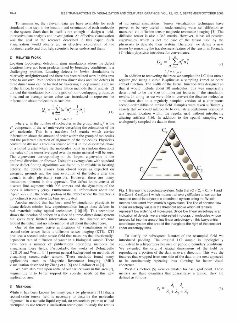
Fig. 1. Barycentric coordinate system. Note that (Cl + Cp + Cs) = 1 and 0<=Cl<=1, 0<=Cp<=1 which means that every diffusion tensor can be mapped onto this barycentric coordinate system using the Westin metrics calculated from matrix’s eigenvalues. The line of constant low linear anisotropy value is the threshold above which all tensors represent low ordering of molecules. Since low linear anisotropy is an indication of defects, we are interested in groups of molecules whose tensors fall into the area of low linear anisotropy on this barycentric coordinate system (the area of the triangle to the right of the constant linear anisotropy line).

To clarify the subsequent features of the resampled field we introduced padding. The original LC sample is topologically equivalent to a hypertorus because of periodic boundary conditions. We extended the original spatial dimensions of the field by reproducing a portion of the data in every direction. This way the features that wrapped from one side of the data to the next appeared to be continuously repeating thus allowing for better visual coherence.

Westin’s metrics [5] were calculated for each grid point. These metrics are three quantities that characterize a tensor. They are defined as follows.

321

21

λλλ

λλ

++

−=lc (3)

1324

SLAVIN ET AL.: TECHNIQUES FOR THE VISUALIZATION OF TOPOLOGICAL DEFECT BEHAVIOR IN NEMATIC LIQUID CRYSTALS

321

32 )(2

λλλ

λλ

++

−=pc (4)

321

33

λλλ

λ

++=sc (5)

where 0321 ≥≥≥ λλλ are the eigenvalues of the tensor matrix. cl is the linear anisotropy measure which describes how ‘cigar like’ the tensor is. cp is the planar anisotropy measure which describes how ‘pancake like’ the tensor is. cs is the isotropy measure which describes how ‘sphere like’ the tensor is [Figure 1].

We calculated Integral paths through the principal eigenvector field to create streamtubes in regions with sufficient linear anisotropy [6]. These streamtubes represent the average molecular orientation in regions outside topological defects. Because the defects occur where the relative ordering of molecules is very small, we expected small linear anisotropy values there and no streamtubes.

Regions of low linear anisotropy can represent defects and can be visualized by plotting isosurfaces of linear anisotropy values. Defects form closed linear structures and so these isosurfaces are tori [Figure 2]. The anisotropy value chosen was varied to produce the desired visualization effect as the linear anisotropy value changed the diameter of the tube comprising the surface [Figure 4].

Fig. 2. Defects as isosurfaces. The visualization of the resulting data included streamtubes (red tubes representing the directions of higher linear anisotropy values) and isosurfaces (blue hollow tubes representing areas of constant low linear anisotropy values and hence candidates for topological defects). The meshes were generated in the OpenInventor format and were loaded in a scene viewer that allowed for basic mouse and keyboard manipulations.

Because low linear anisotropy is a necessary but not sufficient condition for a true topological defect, these were only possible locations of the defects. However, examination of the structure of the streamtubes in the neighborhood of the defects indicates that they are in fact true topological defects. Defects in nematic liquid crystals are characterized by streamtubes that pass through the interior of the defect loop and then double back in their original direction. This can be seen in Figures 2 and 7.

LC physicists are particularly interested in the structure of the core of the defect, i.e. the spatial region within the blue defect tubes. Therefore, we introduced more tools to allow for more detailed exploration. We augmented the visualization of the tensor field features with color-coded cutting planes that display the values of the Westin metrics at various locations in the system. We also mapped the values of the Westin metrics onto the isosurfaces forming the tubes. We enhanced this feature by introducing a tool to probe the

values of the field, which allowed for quantitative analysis of the Westin metrics at areas of interest [Figure 3].

Fig. 3. AVS visualization. The visualization in AVS includes low linear anisotropy isosurfaces as well as color-mapping of planar anisotropy or isotropy scalar fields onto the isosurfaces (top) and arbitrary slice plane (bottom). A probe was also introduced which allows for more precise measurement of these scalar fields. This introduces a high level view of the data with the ability to probe the data in more detail at areas of interest. Compared with the approach described in Figure 2, this visualization adds more interactivity to the exploration of data. It does not replace streamtubes and isosurfaces visualization but augments it by showing the same LC defect scenario for a different level of data analysis.

Such explorative and interactive framework for tensor data analysis allows the researchers to map a variety of different data parameters onto the visual representation of their data. This effectively increases the dimensionality of the visualization. Many more data dimensions can be visualized in context with each other than previously was possible. The researchers can pick and choose which features of the defect data they want to explore. They can map defects data parameters to the surface color of the objects or to the plane slicing through the data volume. This allows them to visually query their data for any point inside their volume of data [Figure 3].

The above tools were built to analyze only one time step. By stitching together the visualization environments as frames of a movie we were able to build an animation of the evolution of the system.

4 RESULTS AND DISCUSSION

The data used for the visualization is the snapshot of the LC system at a time step in the simulation where the defects are well separated from each other [2]. The system consists of ~64K molecules each represented by a second-order 3D tensor at a particular location.

1325


Two of the authors (RP and AC-J) are physicists who used these new approaches and provide the following feedback.

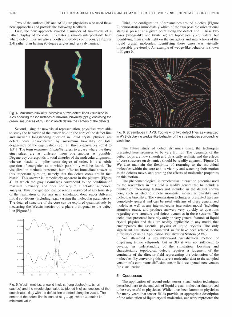
First, the new approach avoided a number of limitations of a lattice display of the data. It creates a smooth interpolatable field where defect lines are also smooth and evolve continuously [Figures 2,4] rather than having 90 degree angles and jerky dynamics.

Fig. 4. Maximum biaxiality. Sideview of two defect lines visualized in AVS showing the isosurfaces of maximal biaxiality (gray) enclosing the green isosurfaces of Cl = 0.12 which define the centers of the defects.

Second, using the new visual representation, physicists were able to study the behavior of the tensor field in the core of the defect line and answer a longstanding question in liquid crystal physics: are defect cores characterized by maximum biaxiality or total degeneracy of the eigenvalues (i.e., all three eigenvalues equal to 1/3)? The term maximum biaxiality refers to a case where the three eigenvalues are as different from one another as possible. Degeneracy corresponds to total disorder of the molecular alignment, whereas biaxiality implies some degree of order. It is a subtle question of energetics as to which possibility will be found. The visualization methods presented here offer an immediate answer to this important question, namely that the defect cores are in fact biaxial. This answer is immediately apparent in the pictures [Figure 4], in which the gray isosurfaces correspond to the condition of maximal biaxiality, and does not require a detailed numerical analysis. Thus, the question can be readily answered at any time step of the simulation or for any new simulation done under different initial conditions (including, e.g., varying the molecular parameters). The detailed structure of the core can be explored quantitatively by measuring the Westin metrics on a plane orthogonal to the defect line [Figure 5].

Fig. 5. Westin metrics. cl (solid line), cp (long dashed), cs (short dashed) and the middle eigenvalue λ2 (dotted line) as functions of the coordinate axis y with the defect line oriented along the z axis. The center of the defect line is located at 40y ≈ , where cl attains its minimum value.

Third, the configuration of streamtubes around a defect [Figure 2] demonstrates immediately which of the two possible orientational states is present at a given point along the defect line. These two cases (wedge-like and twist-like) are topologically equivalent, but identifying them sheds light on the energetics and interactions of the liquid crystal molecules. Identifying these cases was virtually impossible previously. An example of wedge-like behavior is shown in Figure 6.

Fig. 6. Streamtubes in AVS. Top view of two defect lines as visualized in AVS displaying wedge-like behavior of the streamtubes surrounding each line.

The future study of defect dynamics using the techniques presented here promises to be very fruitful. The dynamics of the defect loops are now smooth and physically realistic and the effects of core structure on dynamics should be readily apparent [Figure 7]. We also maintain the flexibility of returning to the individual molecules within the core and its vicinity and watching their motion as the defects move, and probing the effects of molecular properties on this motion.

The phenomenological intermolecular interaction potential used by the researchers in this field is readily generalized to include a number of interesting features not included in the dataset shown here, such as electric dipole moments, molecular chirality and molecular biaxiality. The visualization techniques presented here are completely general and can be used with any of these generalized models, as well as any intermolecular interaction model (including atomistic ones), and produce answers very quickly to questions regarding core structure and defect dynamics in these systems. The techniques presented here rely only on very general features of liquid crystal physics and thus are readily applicable to any model that encompasses the essential physics of liquid crystals. The only significant limitations encountered so far have been related to the difficulties of using Application Visualization System (AVS).

We attempted a straightforward visualization method of displaying tensor ellipsoids, but in 3D it was not sufficient to develop an understanding of the simulation. Locating and characterizing topological defects requires a judgment of the continuity of the director field representing the orientation of the molecules. By converting this discrete molecular data to the sampled version of a continuous diffusion tensor field we opened new venues for visualization.

5 CONCLUSION

The application of second-order tensor visualization techniques described here to the analysis of liquid crystal molecular data proved to be very useful to physicists. While it has been known to physicists for many years that tensor fields provide an appropriate description of the orientation of liquid crystal molecules, our work represents the

1326

SLAVIN ET AL.: TECHNIQUES FOR THE VISUALIZATION OF TOPOLOGICAL DEFECT BEHAVIOR IN NEMATIC LIQUID CRYSTALS

first application of tensor field visualization techniques to liquid crystal physics. The present method was validated by comparing the results found for the location of the defect lines with an earlier method. Furthermore, the defect lines found using both the earlier and present methods obey the nontrivial physical requirement of forming closed loops which shrink over the course of time. Defect lines were never observed to suddenly appear or disappear. The present techniques have a number of strong advantages compared to the previous approach used by physicists. The defect loops have a more natural, smooth appearance leading to useful animations. In addition, the new techniques allow the study of the internal structure of defect cores and the nature of the molecular orientation surrounding the defects which was impossible using earlier techniques. These results are further illustrated in the Figures 8 to 11.

Fig. 7. Close-up of isosurfaces representing defects. This collection of blue-colored isosurfaces formed closed loops (topological defects). The streamtubes flowing through and around them lie in the directions of higher linear anisotropy values above a certain threshold. The close-up of the loop structure (blue) reveals the details of the behavior of the system around the vicinity of the defect (the core). Because the streamtubes (red) are appropriately spaced out, the user can zoom in and effectively explore the cores of the easily identifiable defects.

REFERENCES

[1] Robert Pelcovits, Jeffrey Billeter, “Simulations of liquid crystals”, Invited article, Computers in Physics, 12, 440, 1998.

[2] Jeffrey L. Billeter, Alexander M. Smondyrev, George B. Loriot, Robert A. Pelcovits, “Phase-Ordering Dynamics of the Gay-Berne Nematic Liquid Crystal”, Physical Reiew, E 60, 6831, 1999.

[3] D.H. Laidlaw, E.T. Athens, D. Kremens, M.J. Avalos, R.E. Jacobs, C. Readhead, “Visualizing diffusion tensor images of the mouse spinal cord”, Proc. of IEEE Visualization, pp. 127-134, 1998.

[4] Carolina Cruz-Neira, Daniel J. Sandin, Thomas A. DeFanti, “Surround-Screen Projection-Based Virtual Reality: The Design and Implementation of the CAVE”, Proc. Computer Graphics Siggraph, pp. 135-142, 1993.

[5] C.-F. Westin, S. Peled, H. Gudbjartsson, R. Kikinis, F. A. Jolesz, “Geometrical Diffusion Measures for MRI from Tensor Basis Analysis”, Proc. Int’l Soc. Magnetic Resonance in Medicine (ISMRM), 1997.

[6] S. Zhang, C Demiralp, D.H. Laidlaw, “Visualizing Diffusion Tensor MR Images Using Streamtubes and Streamsurfaces”, IEEE Transactions on Visualization and Computer Graphics, 9(4):454-462, 2003.

[7] V.A. Slavin, D.H. Laidlaw, R. Pelcovits, S. Zhang, G. Loriot, A. Callan-Jones, “Visualization of Topological Defects in Nematic Liquid Crystals Using Streamtubes, Streamsurfaces and Ellipsoids”, IEEE Visualization, pp 21p - 21p, 2004.

[8] J.G. Gay, B.J. Berne, “Modification of the overlap potential to mimic a linear site-site potential”, J. Chem. Phys., 74, 3316-3319, 1981.

[9] J. Crain, A.V. Komolkin, “Simulating molecular properties of liquid crystals”, Advances in Chemical Physics, 109, 39-113 (1999).

[10] Chiccoli, Feruli, Lavrentovich, Pasini, Shiyanovskii, and Zannoni, “Topological defects in schlieren textures of biaxial and uniaxial nematics”, Physical Review E 66 (3): Art. No. 030701 Part 1, 2002.

[11] P.G. deGennes and J. Prost, The Physics of Liquid Crystals, Clarendon Press, Oxford, 1993.

[12] T. Delmarcelle, L. Hesselink, “Visualization of second-order tensor fields with hyperstreamlines”, IEEE CG&A 13(4):25-33, July 1993.

[13] T. Delmarcelle, “The Visualization of Second-Order Tensor Fields”, PhD thesis, Stanford Univ., Stanford, Calif., 1994.

[14] C.-F. Westin et al, “Processing and visualization for diffusion tensor MRI”, Medical Image Analysis 6, pp 93-108, 2002.

[15] S. Mehta, K. Hazzard, R. Machiraju, S. Parthasarathy and J. Wilkins, “Detection and Visualization of Anomalous Structures in Molecular Dynamics Simulation Data”, Proc. of IEEE Conference on Visualization, Austin, Texas, pp 475-462, 2004.

[16] Oppenheimer, Willsky, and Young, Signals and Systems, Prentice-Hall, 1983.

1327


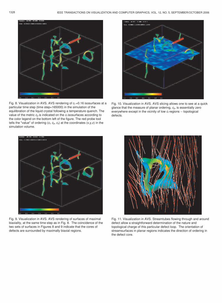
Fig. 8. Visualization in AVS. AVS rendering of cl =0.16 isosurfaces at a particular time step (time step=165000) in the simulation of the equilibration of the liquid crystal following a temperature quench. The value of the metric cp is indicated on the cl isosurfaces according to the color legend on the bottom left of the figure. The red probe tool tells the "value" of ordering (cl, cp, cs) at the coordinates (x,y,z) in the simulation volume.

Fig. 9. Visualization in AVS. AVS rendering of surfaces of maximal biaxiality, at the same time step as in Fig. 8. The coincidence of the two sets of surfaces in Figures 8 and 9 indicate that the cores of defects are surrounded by maximally biaxial regions.

Fig. 10. Visualization in AVS. AVS slicing allows one to see at a quick glance that the measure of planar ordering, cp, is essentially zero everywhere except in the vicinity of low cl regions -- topological defects.

Fig. 11. Visualization in AVS. Streamtubes flowing through and around defect allow a straightforward determination of the nature and topological charge of this particular defect loop. The orientation of streamsurfaces in planar regions indicates the direction of ordering in the defect core.

1328

techniques for the visualization of topological defect...

Documents