PREVIOUSLY ISSUED NUMBERS OF BRUEL & KJ/ER TECHNICAL REVIEW

4-1982 Sound Intensity (Part II Instrumentation and Applications) 3-1982 Sound Intensity (Part I Theory). 2-1982 Thermal Comfort. 1-1982 Human Body Vibration Exposure and its Measurement. 4-1981 Low Frequency Calibration of Acoustical Measurement

Systems. Calibration and Standards. Vibration and Shock Measurements.

3-1981 Cepstrum Analysis. 2-1981 Acoustic Emission Source Location in Theory and in Practice. 1-1981 The Fundamentals of Industrial Balancing Machines and their

Applications. 4-1980 Selection and Use of Microphones for Engine and Aircraft

Noise Measurements. 3-1980 Power Based Measurements of Sound Insulation.

Acoustical Measurement of Auditory Tube Opening. 2-1980 Zoom-FFT. 1-1980 Luminance Contrast Measurement. 4-1979 Prepolarized Condenser Microphones for Measurement

Purposes. Impulse Analysis using a Real-Time Digital Filter Analyzer.

3-1979 The Rationale of Dynamic Balancing by Vibration Measurements. Interfacing Level Recorder Type 2306 to a Digital Computer.

2-1979 Acoustic Emission. 1-1979 The Discrete Fourier Transform and FFT Analyzers. 4-1978 Reverberation Process at Low Frequencies. 3-1978 The Enigma of Sound Power Measurements at Low

Frequencies. 2-1978 The Application of the Narrow Band Spectrum Analyzer Type

2031 to the Analysis of Transient and Cyclic Phenomena. Measurement of Effective Bandwidth of Filters.

1-1978 Digital Filters and FFT Technique in Real-time Analysis. 4-1977 General Accuracy of Sound Level Meter Measurements.

Low Impedance Microphone Calibrator and its Advantages. 3-1977 Condenser Microphones used as Sound Sources. 2-1977 Automated Measurements of Reverberation Time using the

Digital Frequency Analyzer Type 2131. Measurement of Elastic Modulus and Loss Factor of PVC at High Frequencies.

(Continued on cover page 3)

TECHNICAL REVIEW No. 1 — 1983

Contents

System Analysis and Time Delay Spectrometry by H. Biering and O.Z. Pedersen 3

Addendum to Sound Intensity (Part II. Instrumentation & Applications) printed in Technical Review No.4 - 1982 52

SYSTEM ANALYSIS and TIME DELAY SPECTROMETRY (Part I)

by

H. Biering, M.Sc. and

O.Z. Pedersen, M.Sc.

ABSTRACT

Time Delay Spectrometry (TDS) is a relatively new method for measurement of system response. Based on a linear sine sweep it optimizes measurement performance eliminating some earlier drawbacks of swept measurements. By its very nature this method tempts us to adopt an identical complex description in the time and frequency domains. To fully utilize the benefits from this descrip­tion it is essential to consider the general behaviour of two-port systems and the problems encountered in the measurement of these.

The present part of the article is an overview of the theoretical foundation for analysis of linear and time invariant systems. Part II deals more specifically with the TDS technique and its practical implementation.

SOMMAIRE

La Spectrometrie a filtrage decale (TDS) est une methode relativement recente pour la mesure de la reponse des systemes. Basee sur un balayage sinusoidal lineaire, elle optimalise la mesure des performances en eliminant quelques inconvenients des mesures par balayage. De par sa nature meme, cette me­thode nous incite a adopter une description complexe identique dans les domaines temps et frequence. Pour ben^ficier pleinement de cette descript ion, il est essentiel de considerer le comportement general des syst&mes a deux portes et les problemes que Ton rencontre lorsqu'on les mesure.

Cette premiere partie de I'article nous donne une vue generale des fondements theoriques de I' analyse de systemes lineaires et in variables en temps. La deuxi^me partie traite plus particuli&rement de la technique TDS et de sa realisation pratique.

3

ZUSAMMENFASSUNG

Time Delay Spectrometry (TDS) ist eine relativ neue Methode zur Messung der Eigenschaften von Systemen. Die Messung basiert auf einer linearen Sinus-durchstimmung und ist optimiert, so dafi einige der Nachteile durchgestimmter Messungen Darstellung im Frequenz- sowie im Zeitbereich zu benutzen. Um die Vorteile dieser Darstellung vollkommen auszunutzen, ist die Berucksichtigung des allgemeinen Verhaltens von Vierpolsystemen und den Problemen bei der Messung an diesen notwendig.

Der vorliegende Teil des Artikels gibt einen Uberblick der theorethischen Grund-lagen des Systems fur die Analyse von linearen, zeitunabhangigen Systemen. Teil 2 befafM sich eingehender mit der TDS-Technik und ihrer praktischen Anwendung.

1. Introduction

For characterizat ion of linear systems in the t ime domain the real-valued impulse response has been the tradit ional choice. However, very little information can be gained directly f rom watching this repre­sentation of the data. Furthermore, due to the instrumentat ion hitherto available, frequency domain descript ions have been prevail ing in the past.

The principal advance associated with Time Delay Spectrometry (TDS) is the straightforward way by which a useful data representat ion in the t ime domain can be obtained. The possibi l i t ies of TDS were first described in 1967 by R.C. Heyser in Ref.[1]. A later article by the same author [2] is a good supplement to the original paper. Heyser intro­duces his improved t ime domain representat ion along with a new energy definit ion. As a consequence of this he refers to the measured results as Energy Time Curves (ETC).

However we have chosen to refer to this representat ion as the Time Response as it is a true analogue to the Frequency Response, the most commonly used and understood frequency domain representat ion.

In the choice of both terminology and examples for this text the similarit ies between frequency and time domain descript ions have been stressed. Most of the widespread theoretical and empir ical knowledge available for interpretat ion of frequency response can be translated for use in the time domain. The transfer of already recognised knowledge from one domain to the other, effectively el iminates the need for

4

creating a separate theoretical foundation for the Time Response, and provides a desirable short cut to a thorough understanding of time domain phenomena.

TDS has more advantages when compared with other techniques for measurement of system response. In [4] it is shown that TDS out performs any other technique with respect to suppression of correlated and uncorrelated noise. Furthermore non-linearities are not only sys­tematically excluded from affecting the measurement of linear behav­iour - if desired they can also be extracted and treated separately.

2. Description of Time and Frequency Domain Phenomena The human perception of "frequency" and " t ime" is a highly complicat­ed physiological process eluding exact analysis using the mathematical tools we presently have at hand. Basically, however, we note that when we deal with the concept "frequency" we intuitively inverse the units used for description of "time domain" phenomena. We either ask "when" expecting an answer in terms of minutes and seconds or "how often" if we prefer the units rpm and Hz.

This leads us to a simplif ied model defining frequency and time as a Fourier Transform couple [3]. In the acoustical field this model was introduced by Helmholtz in 1862.

If A(f) = f a(t) e~}2zftdt (2.0.1)

a n d a(t) = I A(f) eJ2*ft df (2.0.2)

then a{t) « * A(f) (2.0.3)

According to this definition any event that can be associated with a time signal (time domain representation) can equally well be described in terms of the corresponding spectrum (frequency domain representa­tion). The reversibility of the transform ensures that these representa­tions are always equivalent descriptions of the event.

From the definition it is seen, that in principle, estimation of a single frequency component requires a global knowledge of the time signal and vice versa. This fact alone makes it clear that frequency thus

5

defined is not consistent with the "frequency" of human perception -often referred to as pitch. Clearly pitch is a function of time, but frequency is not — by definition.

What is even more critical is that the transform cannot be used for real life events on account of integration to infinity. To overcome this problem we are forced to modify the events by imposing time and frequency "windows" on their respective representations. If this is done properly, the Fourier Transform can be used to predict to a certain extent the response of human beings, machinery etc. to the events. Choice of "windows" and representation is discussed in Section 4.

2.1. General Properties of the Fourier Transform The discipline of Fourier analysis has been treated very well and thoroughly by several authors. For an extensive study [5] and [6] can be recommended. Most of the present works are, however, somewhat unilateral in their description of the two domains, time and frequency. Therefore one may be tempted to believe that time signals should always be considered real-valued whereas spectra are naturally complex.

A closer study reveals that there is no reason for this distinction. One purpose of this article is to draw attention to this point through a

Fig. 2.1. An arbitrary (also complex) function can be regarded as a sum of an even function and an odd function. Generally there is no specific bond between these two parts

6

discussion of some basic properties of the Fourier Transform. The fundamental symmetry between the two domains is readily seen from the definition.

If a(t) - * A(f)

then also A(f) « > a(-t)

We see that there is no mathematical reason to prefer either time or frequency domain description of an event. The preference must depend upon the nature of the actual event.

Any function, f(x), (see Fig.2.1) can be regarded as a sum of two functions fe(x) and f0(x) where

fefr) = fe(-X) and f0{*) = -fo(-X)

We refer to fe(x) as an even function and to f0(x) as an odd function.

With these definitions we can derive another basic Fourier Transform property. The relationships shown in Fig.2.2 apply to any Fourier Transform pair. It is seen that the even parts of the response are

t J

Fig. 2.2. The separation of a function in real and imaginary, even and odd parts is often convenient. Use of the relationships indicat­ed in the figure facilitates Fourier Transform calculations by replacing complex and infinite integration with real and semi-infinite integration

7

preserved real and imaginary respectively. Odd real parts are trans­formed to odd imaginary parts and vice versa. These relationships are often utilized to simplify practical Fourier Transform calculations.

2.2. The Hilbert Transform It will be shown later that the function

1 for x 0 sgn(x) = (2.2.1)

1-1 for x - 0

is very useful for modif ication of signals and spectra in conjunction with Fourier Analysis. Some properties associated with this function will therefore be mentioned. Much of the mathematical foundation for this " tool" was provided by the german mathematician Hilbert and various aspects of the Hilbert Transform are discussed in [5].

We find the following Fourier Transform relationships

sgn(f) * - -j/wf (2.2.2)

j/ir t « > s g n ( f ) (2.2.3)

The Hilbert Transform, ^ \a(x)}, of the function a(x) is defined as the convolution integral of a(x) with (1 / TT X ) . We express this by:

a(x) « ► a(x) • (1 / - x) (2.2.4)

It is readily seen that in contrast to the Fourier Transform the Hilbert Transform is a local to local mapping within either the time domain or the frequency domain. To derive some important properties of the Hilbert Transform we rewrite equation (2.2.2)

r elrJ7 for f ■ 0 \ v

y s g n ( f ) = I f * 1 / r r f

I e~Jz/2 for r 0 J (2.2.5)

From equation (2.2.3) we obtain similarly

: z ( e / T / 2 for f 0 1/Trf < - -jsgn(f) - I (2.2.6)

I eSr"'2 fo r f- 0

8

As in both domains the Hilbert Transform is equivalent to a phase shift of + TT/2 in the alternative domain, we find

# ? { a(x)\ = )f \ a(x)} * ( 1 / T T X ) = - a ( x ) (2.2.7)

and thus also

* 4{a(x)\ = a(x) (2.2.8)

where the indices # 2 and % 4 refer to two and four successive Hilbert Transforms.

Equations (2.2.5) and (2.2.6) are useful for evaluation of the Hilbert Transform. Combining these with the defini t ion of the Fourier Trans­form we find that in both domains the Hilbert Transform of a function

a(x) = A}(y) cos2 ; r xy dy + A 2(y) sin 2K xydy (2.2.9) Jo Jo

can be expressed

#\a(x)}= ) A,(y) sin 2n xydy - J A2(y) cos 2TT xydy (2 .2 .10)

i i i l

( ^ ■ i ' -* • i

L - —i

Fig. 2.3. Unlike the Fourier Transform the Hilbert Transform maps a function in one domain into another function in the same domain

9

It is seen that the Hilbert Transform bears resemblance to integration and differentiation. These operations however further involve multipl i­cation or division with the variable 2TT y. If A^(y) and A2(y) only take significant values within a narrow range, y can be considered a con­stant. In this case #\a(x)\ will be directly proport ional to both the integral and the derivative of a(x) .

As the operator (MKX) is a real-valued odd function we obtain the relationships shown in Fig.2.3. Real and imaginary parts are not mixed, but even parts are transformed into odd parts and vice versa.

As stated earlier we can never apply the Fourier Transform directly to real life events without a certain "windowing" of their representations. Typically it is the limited time or frequency range we have available for a measurement that calls for modif icat ion of an event. If we base the representation in the time domain on the range from 0 to T, i.e. we multiply the original response with

a ( 0 = 1/2 ( s g n ( f ) - s g n ( f - T ) ) (2.2.11)

the corresponding spectrum will be convolved with the function

1 e - y 2 i r r f _ - |

A(f) = - y ( ^ - e - i 2 l ^ T f ) = 2irf V ' -j2irf

sin(2 7r Tf) COS(2TT T f ) -1 +y (2.2.12)

2irf 2ivf

If alternatively the spectum is limited to the interval from 0 to F, i.e. we multiply the original response with

B(f) = 1/2 ( s g n ( f)-sgn( f-F) ) (2.2.13)

the result is a convolution of the time domain representation of the original event with the function

b(t)=

j2irt

$\n(2irFt) C O S ( 2 T T F 0 - 1 = -j (2.2.14)

2>rf 2izt 10

Fig. 2.4. When a signal or spectrum is modified by multiplication with a "window", the alternative representation of the event is con­volved with a complex function. For reasons mentioned in Section 3, we refer to the even real projection of this function as a coincident or impulse part and to the odd imaginary projection as the quadrature or doublet part

Fig.2.4 is a three dimensional plot of the complex function (ei2*Ab-1)/j2w b. The envelope of this function depends on the value of A, i.e. the extension of the "window" in the alternative domain. This is illustrated in Fig.2.5. It is seen that the Fourier Transform of the wider "window" (right hand side of the figure) has its energy concentrated closer to the origin.

Letting F -oo and T -oo i.e.

B(f) M / 2 J 1 + sgn(f)) (2.2.15)

and a(t) - 1 / 2 ( 1 + sgn(f)) (2.2.16)

we approach the idealized operators

b ' ( 0 = 1/2 (o(t) + jd(t)) (2.2.17)

11

Fig. 2.5. Extension of the window range leads to a more narrow repre­sentation in the alternative domain - here illustrated by the envelope of the complex function in Fig.2.4

and Aco(f) = M2 [h(f)-jd(f)) (2.2.18)

referring to h{t) as the unit impulse or coincident operator and d(t) as the doublet or quadrature operator

* _ _ ■ ■ ■ _ . - _- - _ ^ j

Fig. 2.6. Tending towards a semi-infinite frequency or time range the projections of the Fourier Transform approach the idealized operators S(x) and d(x)

12

These idealized operators are sketched in Fig.2.6.

The operators 2bco(t) and 2Acn(t) are the generating functions for obtaining the so-called analytical (one-sided complex) signals and spectra from the respective real-valued and one-sided representations.

With a proper definition of energy it can be shown, that if a real-valued signal represents, for example, the potential energy of a system, the analytical signal will represent the total energy of the same system. The mutually Hilbert transformed real and imaginary parts of this signal relates to the potential and kinetic energy respectively. This matter is extensively discussed in [2].

In section 3.4 and Appendix A we will see that the Hilbert Transform can be expressed in other equivalent ways. In many cases it is advanta­geous or even necessary (if the convolution integral a(x) • 1/x does not exist) to use one of the alternative expressions for ,ff{ a(x)}.

3. System Response The Fourier and Hilbert Transforms introduced in Section 2 can be directly applied to optimize the description of any event for which the relevant integrals exist.

System analysis where the object is to measure the relation between an input, x , and a correlated output, y, is a far more complicated matter. If we want to restrict mathematics to a reasonable level we must first of all make the sometimes dubious assumption of linearity.

If mH(Xi) + nH(x2) = H(mx, + nx2) (3.0.1)

where x^ and x 2 represent arbitrary events and m and n are arbitrary constants then the system response H is said to be linear. This means that the output corresponding to a linear combination of inputs must equal the sum of outputs due to the individual inputs.

3.1. Time Invariance Generally the response of a physical system will be a function of both time and frequency. As a simple example of this we can consider an audio amplifier which is periodically switched "On" and "Off". The output of the amplifier for a certain test signal input will strongly depend on whether or not the amplifier is "On" when the signal is

13

Fig. 3.1. System analysis is a more complex matter than signal analysis

applied. If the signal is applied while the amplifier is "Off" we can wait forever without getting a correlated output.

With the simple one dimensional Fourier Transform we cannot handle systems like this. We can only define the frequency response, HT(f), of a device if there is an interval in time where the system response, H{t, f), can be considered independent of the actual moment of excita­tion, i.e. H(t,f) = Hr(f). If this condition is fulfilled we refer to the system as being time invariant within the interval T.

As our definition of the frequency response requires that the system response be independent of time, it should be clear that a Fourier Transform of the frequency response function HT(f) does not lead to a time domain description of the system. To benefit from the advantages of the Fourier Transform it is necessary to introduce a new domain

Fig. 3.2. For time invariant systems the delay domain provides a "time­like" alternative to the frequency domain description

14

which we will refer to as the (time) delay domain. To distinguish delay response from time signals we will normally use the parameter r to characterize the representation in the delay domain. The relationship between time, frequency and time delay for time invariant systems is shown in Fig.3.2.

The non-symmetrical input/output relationships:

Y(f) = HT(f)- X(f) (3.1.1)

and y(t) = hT(t) * x(t) = I hT(r) x(t-r)dr (3.1.2)

where x(t) and y(t) are the input and output signals; X(f) , V(f), the

corresponding spectra and hT(r)< > Hr(f), are consequences of the assumption of time invariance.

Equation (3.1.2) shows that the output of a system is not only a function of the present input signal but also of the past. We say that the system has time domain memory. Conversely we see that the output of a linear and time invariant system cannot contain frequency components which are not input to the system.

In this article we will consider the measurement of time invariant systems only.

3.2. Causality In Section 2.1 it was mentioned that any function, f(a), can be regarded as a sum of an even function, fe(a), and an odd function f0{a), If f(a) is a real-valued causal function, i.e. f(a) = 0 for a < 0 we get:

fe(a)= fe(~a) = 1(a) 12 \ > where a > 0 (3.2.1)

fo(3) = -f0(-a)= f(a)/2 J

It is readily seen, (Fig.3.3) that

f0(a) = s g n ( a ) fe(a) (3.2.2)

Using the relationships given in Fig.2.2, (3.2.2) implies that the Fourier Transform, F(£>), of f(a) has an even real part and an imaginary odd part that are mutually related by a Hilbert Transform. Fig.3.4.a and 3.4.b

15

Fig. 3.3. The even and odd parts of a causal function are closely related to each other

illustrate the two symmetrical cases where we assume that either the time domain representation or the frequency domain representation is real-valued and causal.

Fig. 3.4.a. The traditional assumption of impulse response causality leads to a two-sided, complex frequency domain description

16

L . . 1

Fig. 3.4.b. If alternatively a real-valued and causal frequency domain description is prescribed a complex time response must be accepted

If alternatively our starting point is a one-sided analytical representa­tion, f(a), where the real part, fr{a), and the imaginary part, f,(a), form a Hilbert Transform pair and

fr(a) — F,(b) (3.2.3)

then ff(a) «-- - F2(b) = ±ysgn(to) ■ F^{b) (3.2.4)

indicating that the complete representation F(b) = F, {b) T F 2 (b) isone-sided. The one-sidedness of f{a) implies that the real and imaginary parts of F(b) are related by a Hilbert Transform. We conclude that the Fourier Transform of an analytical representation in one domain is the analytical representation of the alternative domain, and that for these representations, one-sidedness in one domain implies one-sidedness also in the alternative domain. Fig.3.5 shows the relationship between the analytical representations in the time and frequency domain.

Note that either of the four representations indicated by the circles can be used to generate the others. This means that any of the representa­tions provides a complete description of the system response. As the

17

Fig. 3.5. The analytical response is complex but one-sided in both domains. From any of the four partial representations the other three can be derived

one-sided representations are uniquely related to the corresponding even and odd parts, each of these can also be regarded as a valid and complete representation.

If we restrict ourselves to analysis of systems with causal impulse response, f(r), the Fourier Transform, F(f), can be considered a special case of the more general Laplace Transform defined by

FL(s) = f e~Sr f(r) dr (3.2.5)

where s is a complex variable.

For systems that are stable the transfer function FL{s) will have a continuous derivative for Re(s) ^ 0. We say that FL(s) is analytic in this region of the complex s-p lane. In this case FL(s) and F(f) are related by the equations

FL(s) = F ( ^ — ) or F(f) = FL(j2irf) (3.2.6) j2n

We have already shown that for a causal f(r) the real and imaginary parts of its Fourier Transform, F(f), form a Hilbert Transform pair.

18

Using Cauchys integral theorem we can generalize this relationship between real and imaginary parts to hold for any function F(f) for which the corresponding function FL(s) fulfils the requirements. a. FL(s) is analytic for Re(s) > 0 b. FL(s) has only discrete poles for Re(s) = 0 c. FL{s) ^0 for s *oo

If the latter condition is not fulfilled, but FL(s) »k for s *oo or FL(s) ► ks for s *oo the Hilbert Transform relationship will still be valid except for trivial additions of these terms to either the real or the imaginary part.

In case f(r) contains an impulse, k0 />(r), at the origin, then FL{s) >k0

for s *oo and as k0 is real we obtain the Hilbert Transform relationships:

1 r . Ff-(0) Fr(f) = k0 + - d<!> (3.2.7)

IT J~ • f—(/>

F,(f)= - - -!— d<l> (3.2.8) 7T •/" ' f — 0

where Fr(f) and F,-(f) denote the real and imaginary parts of F(f). For a physical system k0 will always equal zero.

As none of the conditions a to c ensures the existence of the integral

f F(f) ej2*ftdf

we conclude that Hilbert Transform relationship between the real and imaginary parts of a function F(f) does not imply that F(f) is the frequency domain representation of some causal system response.

Due to the symmetry between frequency and time domains we may also conclude that a given complex time response function - even if its real and imaginary parts form a Hilbert Transform pair - may not have a frequency domain representation.

3.3. Magnitude and Phase The real and imaginary parts of a complex response form a vector that can equally well be described by its modulus and argument. We define

19

Fig. 3.6. In both domains the response can be expressed in terms of magnitude and phase. In practice, however, this type of repre­sentation has been reserved for the frequency domain

the magnitude and phase of the response as the real and imaginary parts of the natural logarithm to the complex response:

a (x ) + j()(x) = ln(r(x) + y'/'(x)) (3.3.1)

where n (x ) is the magnitude in nepers rel. to 1. 0(x) is the phase in radians r(x) is the real part of the response i(x) is the imaginary part of the response.

Fig.3.6 shows the relationships between r(x) , /(x), n (x) and (t(x).

Throughout the age of frequency analysis, magnitude and phase have been preferred for frequency domain representation. The reason for this particular choice is obvious when looking at Fig.3.7, showing the coincident and the quadrature response as well as the corresponding Bode plot (magnitude and phase) for a typical third octave filter. Although the two representations contain the same information, the Bode plot provides a far better visualization of the data.

For time domain representations, however, the real-valued impulse response has been the prevailing choice in the past. Although this

20

Fig. 3.7. It is difficult to determine the passband and rejection of a filter from the coincident and quadrature representations. The Bode plot (magnitude and phase) provides a much better visualiza­tion of the data

choice is primary a consequence of the specific methods traditionally employed for acquisition of the system response, it has led many people to the conclusion that the frequency domain is generally better suited for human interpretation than the time domain.

In Fig.3.8 the impulse response of a loudspeaker is compared with the magnitude of the time delay representation, also referred to as the Energy Time Curve.

It appears that the real-valued impulse response suffers from exactly the same deficiencies regarding visualization as the coincident fre­quency response. These deficiencies are primarily recognized as

a. difficulties in extracting the envelope of the complex response from only one of its projections.

b. limitation of the effective dynamic range of the measurement to ratios up to typically 1 to 30 or approximately 30 dB.

21

Fig. 3.8. The direct sound and the first reflections from a loudspeaker in a normal listening room. The impulse response plot gives only a slight indication of the most dominant reflections. The magnitude of the time response, however, reveals the exact level and position of all reflections present in the setup

22

Therefore we should not hesitate in introducing time domain magnitude and phase representation, to achieve the same subjective benefits, as this representation has always provided us for frequency domain description.

3.4. Minimum Phase In this sub-section we will discuss the logarithmic representation of the frequency response as a special case of the transfer function ln( FL(s)) where FL(s) is the Laplace Transform of the causal impulse response associated with a physical system.

The logarithmic operation converts zeros for the function FL{s) into singularities for ln(FL(s)). Therefore, if FL(s) has zeros in the half plane given by Re(s)^0, ln(FL(s)) will not be analytic in a region including the imaginary axis. This indicates that generally a(f) and 0(f) are not uniquely related to each other as are the real and imaginary parts of F(f). This further implies that neither the magnitude alone nor the phase alone of a response suffices for a complete description of a physical system. Next it will be shown that we can interpret any physical response as the product of three basically different transfer functions.

Fig. 3.9. A frequency response function F(f) is characterized by the pole/zero configuration of the corresponding transfer-function FL(s). Stable systems have no poles in the right-hand half-plane

23

Fig. 3.10. Relationship between magnitude and phase requires that there be no zeros in the right-hand half-plane. By adding new pole/zero pairs such zeros can be isolated in a separate, trivial part of the transfer function

Consider first the pole-zero configuration of the transfer function, FL(s), shown in Fig.3.9. If we assume that there is a limited number of zeros in the right-hand half plane (Re(s) > 0), we can for each of these assign a similar zero and a matching pole in the left-hand half-plane. This will not affect the transfer function in other points of the s-p lane. We can then separate the response in two factors as shown in Fig.3.10. Note that for symmetry reasons ( n ( f ) = a(-f)) the poles and zeros will always be distributed symmetrically arround the real axis. The transfer function FLa(s) shown to the right can be expressed by its associated frequency response Fa(f)

j2irf + p, j2irf + p2 Fa(f)= (3.4.1)

j2irf-Pi j2irf-p2

where Re(p^) = Re(p2) <0 and lm(py) = -lm(p2)

We readily observe that

<*a(f) = In | Fa(f) | = 0 for -oo<f<oo (3.4.2)

24

Fig, 3.11. Frequency response of a simple allpass system. The phase will always decrease monotonously with frequency

It is also seen that the argument of the numerators steadily decreases while the argument of the denominators simultaneously increases when f is increased. For 0a(f) = / Fa(f) we conclude

doa(f) < 0 for - oo < f < oo (3.4.3)

df

If for symmetry reasons we choose 0a(0) = 0 we have

fia(f) < 0 for f > 0 (3.4.4)

The resulting characteristic is shown in Fig.3.11. Due to the property (3.4.2) we refer to this part of the system response as an allpass function.

The remaining part of the logarithmic transfer function, ln(FLm\{s)), is analytic for Re(s) > 0. Therefore basically a m i (f) and 0m\(f) will form a Hilbert Transform pair. However, as FLm*(s) »0 for s *oo, we generally have ln(FLmi(s)) *-oo for s »oo. More accurately we can describe the behaviour of FLmi(s) by

FLml(s) — k ■ s~b ■ e~as for s *oo=*

' n ( F / _ m i ( s ) ) as-bln(s)-c for s >oo (3.4.5)

as typical for physical systems.

25

Using Cauchys integral theorem we find

2f Cr <V(0) 0m>(f) = -2iraf + — — — d<!> (3.4.6)

7T J o (<l>2-f2)

and

« m . ( f ) = «(0) - c f 0 (3.4.7) 7T JO 0 ( 0 2~f2)

A restricted but easily modified proof of these equations is given in [5].

We see that it is convenient to separate the frequency response, Fmi(f), in two parts:

Fd(f) = e ^ ( f ) + / f , r f | f > (3.4.8)

and Fm(f) = elx™{f) + j0™(f) (3.4.9)

where ad(f) = a(0) , 0d(f) = -2naf (3.4.10)

2f2 Cr 0(<l>) « m ( 0 = ; — — d ( l > (3.4.11)

7T JO 0 ( 0 2 _ f 2 )

2f f«. a ((f)) (>m(f) = — ; —dtfr (3.4.12)

7T JO {<t2-f2)

The response F d ( 0 is equivalent to a pure delay, a, and a frequency independent gain e"(0), see Fig.3.12. As such, F(d) can also be consid­ered a special contribution to the allpass part of a response function. The expressions for am(f) and 0m(f) are not completely symmetrical. This is because we have used the identities am{f) = am{-f) and f}m(f) - ~f)m(-f) in the evaluation of the expressions. It is easy to show that apart from a constant the relation expressed by (3.4.11) and (3.4.12) is exactly equivalent to the Hilbert Transform relationship derived for the real and imaginary parts of the response in Section 3.2. This means that each of the functions am(f) and nm(f) provides a complete characterization of the frequency response Fm(f).

Writing the total frequency response of the system as

F(f) = Fa(f)- Fd(f)- Fm(f) (3.4.13)

26

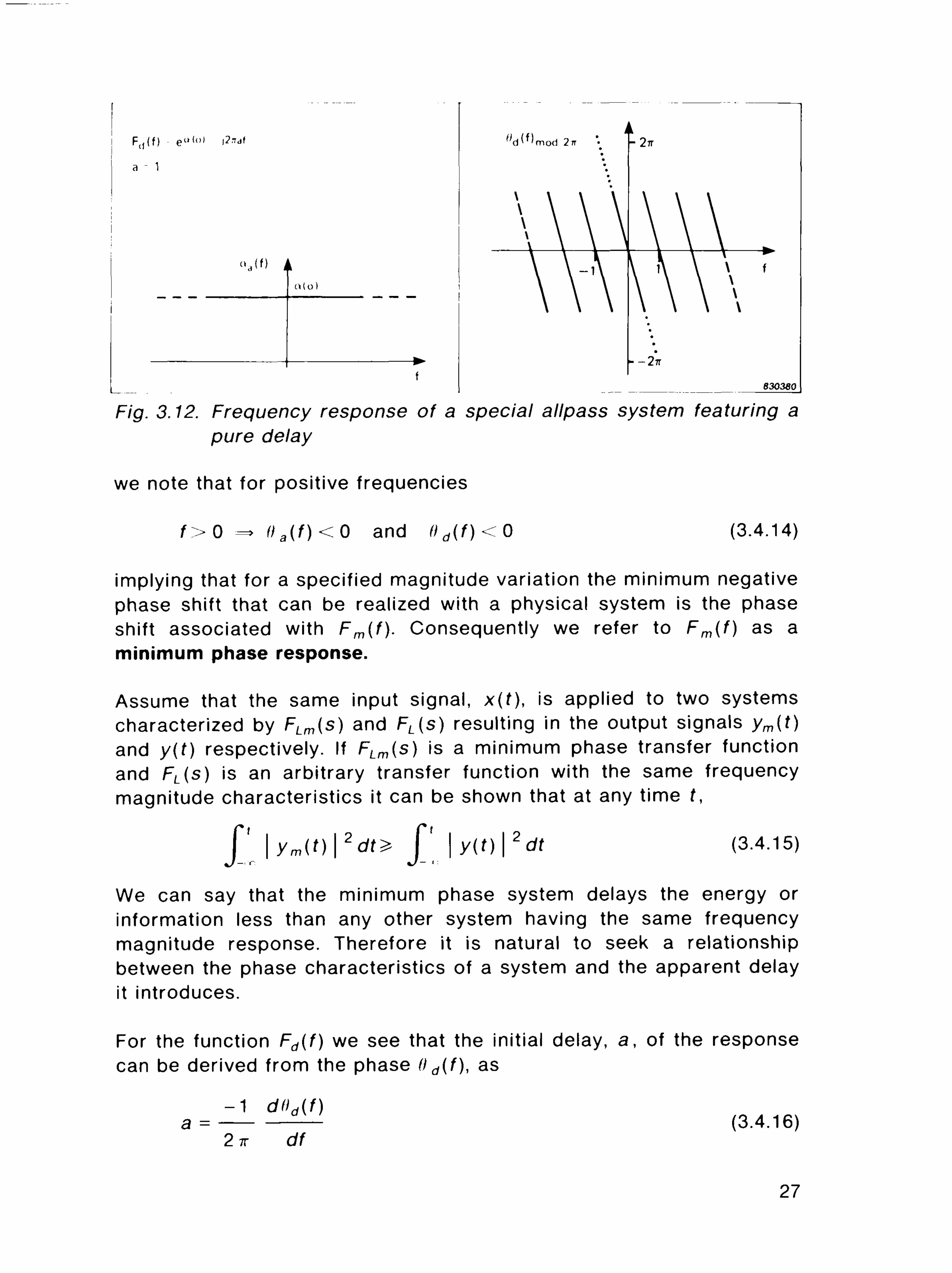
Fig. 3.12. Frequency response of a special allpass system featuring a pure delay

we note that for positive frequencies

f > 0 => 0a(f)<0 and 0d(f)<0 (3.4.14)

implying that for a specified magnitude variation the minimum negative phase shift that can be realized with a physical system is the phase shift associated with Fm(f). Consequently we refer to Fm(f) as a minimum phase response.

Assume that the same input signal, x( f ) , is applied to two systems characterized by FLm(s) and FL(s) resulting in the output signals ym(t) and y(t) respectively. If FLm(s) is a minimum phase transfer function and FL(s) is an arbitrary transfer function with the same frequency magnitude characteristics it can be shown that at any time f,

f \ym(t)\2dt> P \y(t)\2dt (3.4.15) %J- ^ %J- <

We can say that the minimum phase system delays the energy or information less than any other system having the same frequency magnitude response. Therefore it is natural to seek a relationship between the phase characteristics of a system and the apparent delay it introduces.

For the function Fd(f) we see that the initial delay, a, of the response can be derived from the phase 0d(f), as

- 1 dOd(f) a = — (3.4.16)

2TT df

27

This fact has led to the introduction of the concept group delay, defined by

- 1 dfi(f) Tg(f) = (3.4.17)

9 2TT df

Naturally rg{f) is easy to interpret for transfer functions featuring a pure delay. For other all-pass functions rg{f) can also be interpreted as a real delay if it does not vary significantly within the relevant frequen­cy range. For minimum phase systems, however, group delay has no physical meaning as rg(f) can generally be positive as well as negative. Indeed the attempt to describe delay as a function of frequency is a violation of the concept of time delay and frequency as two alternative domains.

To enhance the intuitive understanding of the relationship between (\m(f), 0m(f) and Tgm(f) we can rewrite equation (3.4.12) to obtain a more convenient expression. This is done in Appendix A in Part II of this article.

In most practical systems the modulii of the poles and zeros are distributed in a logarithmic fashion. For this reason we have defined the logarithmic frequency domain variable x = ln<i>lf. With this defini­tion we find

1 r - d<v(0) ex + 1 (>m(f)=— In dx (3.4.18)

7r J- ■ dx ex - 1

- 1 r . d2n(</>) ex + 1

2ir2f J dx2 e* - 1

We see that 0m(f) and rgm(f) are weighted averages of the first and second derivative of am(f). As the weighting coefficient shown in Fig.3.13 goes to infinity at the frequency of interest and decays expo­nentially for x *oo and x * -oo, we note that the transforms can be regarded as local. Unless am(f) has much higher derivatives in other parts of the frequency range, om{f) will be roughly proportional to the slope and rgm(f) to the curvature of am{f). Fig.3.14 shows the frequen­cy magnitude, phase and group delay for two simple minimum phase transfer functions. Note that one of the systems displays negative group delay in part of its frequency range.

28

Fig. 3.13. For a minimum phase system the frequency phase and the group delay are weighted averages of the first and second derivative of the frequency magnitude response. The accu­mulated weighting function shows how the local behaviour of (\(f) dominates the estimate. (Note: logarithmic frequency axis)

We have mentioned that for a given frequency magnitude response the phase shift associated with a minimum phase system will minimize the delay of information. In many cases however, the absolute delay in a system, e.g. a transmission line, is not of prime importance. Often more consideration is paid to the effective duration (read: time smear) of a transmitted pulse. A relevant measure for this duration is, 7"D, the second moment of the power of the impulse response, f{r), about a suitably chosen origin, r0.

TD = min < I r2 f(r-r0) 2 dr > - o o < r 0 < o o [ J~ j (3.4.20)

It can be shown that TD is minimized when rg(f) = d()(f) I df is constant, see Ref.[5].

Consequently a system that minimizes the effective duration of a transmitted pulse is called a linear phase system. True linear phase systems are not generally causal. We can however make a causal

29

Fig. 3.14. Frequency magnitude, phase and group delay for two simple minimum phase systems. Also indicated are the slope and the curvature of the magnitude response. The two latter representations show the same general trends as the phase and group delay, but with exaggerated variation

30

approximation to any such system by adding cautiously allpass proper­ties to a minimum phase system with the desired frequency magnitude response. Fig.3.15 illustrates this approximation.

Fig. 3.15. A linear phase system (A) can be approximated (D) by adding allpass characteristics (C) to a minimum phase system (B) having the proper frequency magnitude response. However, the negative slope of 0D, determining the positon of hD(r) on the T-axis, is downwards limited by the maximum negative slope of fiB

31

No phase compensation, however, will be able to correct the smear introduced by irregularities in the frequency magnitude response. Therefore optimization of the phase response should never be attempt­ed without a simultaneous optimization of the magnitude response.

3.5. Frequency Invariance The description of linear systems evaluated in the previous sections was based on the fundamental assumption of time invariance. Practical systems however, need not obey this assumption.

Let us return to the example in subsection 3.1. Assume that the gain of the amplifier is now varied as a function of time: the amplifier then modulates the input signal causing sidebands in the output spectrum. To determine this time dependent variation of the response correctly we must require that the output spectrum - carrying the evidence of this variation - be confined to some frequency range, F, within which the system response H(t, f) is independent of frequency ( i.e. H(t, f) = HF(t)). Otherwise information will be lost or misinterpreted.

Fig. 3.16. For frequency invariant systems the modulation domain pro­vides a "frequency-like" alternative to the time domain description

32

As our definition of time response requires that the system response be independent of frequency, it should be clear that a Fourier Trans­form of the time response function /-/(f) does not lead to a frequency domain description of the system. To benefit from the advantages of the Fourier Transform it is necessary to introduce a new domain which we will refer to as the (frequency) modulation domain. To distinguish modulation response from frequency spectra, we will choose the pa­rameter <(> to characterize the representation in the modulation domain. The relationship between time, frequency and frequency modulation for frequency invariant systems is shown in Fig.3.16.

Naturally the input - output relationships given in Section 3.1 are now inverted with respect to the time and frequency domains:

y( f ) = HF(t) x(t) (3.5.1)

and

Y(f) = hF(f) * X(f) = j hF(<i>) ■ X(f-<t>)d<l> (3.5.2)

where x(t) and y(t) are the input and output signals, X(f), Y{f) the

corresponding spectra and HF(t) < * hF((i>).

Equation (3.5.2) shows that the output of a system is not exclusively related to input frequency components within the range of the output spectrum. We say that the system has frequency domain memory. Conversely we see that for a linear and frequency invariant system the output signal is only present within the period of excitation.

3.6. General Model, Foundation for TDS Generally physical devices are neither frequency nor time invariant. In subsection 3.5 we varied the gain of an amplifier at a fast rate. Assume that alternatively the tone controls of the same amplifier are varied at an equally rapid rate, i.e. the "frequency response" is now a function of time (or equally well stated: the "time response" is a function of frequency).

In this case the input - output relations of the amplifier cannot be revealed by a one dimensional Fourier Transform model relating only two of the four domains relevant for its description.

33

Theoretically this problem can be overcome by employing a two dimen­sional model where the response is considered a combined function, H(tJ), of time and frequency. We will however only benefit from this model in exceptional cases where the response is known to be a periodic function of either time or frequency. Otherwise we will never be able to measure or predict the output from a system requiring the use of such a model.

For this reason we will seldom abandon the one dimensional model relating either frequency and delay or time and modulation. When frequency or time invariance is clearly established we will often substi­tute time for delay and frequency for modulation.

For the understanding of swept measurements, however, it is essential not to confuse the domains with each other. The foundation for these measurements is the attempt to establish a relation between the time and frequency domains in order to measure the frequency response of a time invariant system as a function of time. In doing so delay is simultaneously converted into modulation as shown in Fig.3.17.

Fig. 3.17. When the frequency response of a time invariant system is measured as a function of time the (time) delay response is converted to a (frequency) modulation function

34

Formerly the frequency shift arising from this conversion was regarded a problem with swept measurements, as very long sweep times were often necessitated. With the conception of Time Delay Spectrometry this apparent drawback suddenly turned out to be an advantage. Richard Heyser Ref.[1], drew attention not only to the possible compen­sation of the undesired frequency offsets, but he also showed that analysis of the modulation spectrum provides a complex description of the impulse response of the system under test.

Sections 5, 6 and 7 of this article are devoted to a detailed description of the TDS technique, its advantages and limitations.

4. Practical Considerations When measuring the response of a two-port system, some practical choices have to be made. The basic choice in any measurement of a system response is the choice of the time range T and the frequency range F. Once F and T have been fixed the maximum amount of information will also be fixed as F T. This information may, however, be expressed in various ways, some of which lend themselves more readily to interpretation. Another practical choice is the choice of the test signal and method of analysis. These choices and their conse­quences will be discussed in some detail in this section with special emphasis on the TDS-Technique.

4.1. Segmentation - Choice of F and T When carrying out a test one must decide, in which frequency range F the device under test should be measured. Such a decision is often based on the intended use of the device and measurement results, or if the goal is to obtain an exhaustive description of the linear perfor­mance, on the actual bandwidth of the device. The selected frequency range, both its width and posit ion, is not only important in itself - it also determines the resolution and characteristics in the time delay domain.

It is quite obvious that the latter approach where we try to describe the system in great detail poses some theoretical diff iculties. The problem is a general measurement dilemma and may be expressed as follows: In order to make a sensible choice of measurement parameters it is necessary to know the system response in advance - in which case there would be no reason to measure it. In practice, to solve this dilemma, a trial and error method must be used increasing the frequen­cy range until no further contributions are observed. Often a certain

35

pre-knowledge of the system will be available and physical intuition of system behaviour can guide us in the initial choice. However, one can never be sure to include all important contributions, and according to the definition of the Fourier Transform, F should be infinitely wide and the integration therefore should be carried out over the entire frequen­cy axis when calculating the time delay response.

In view of these practical difficulties, we simply define the measure­ment by the chosen frequency range F. Thus limiting F will result in deviations from the "true" time delay response. These deviations are often referred to as "errors". However, as it may not even be desirable to measure the "true" response, we will avoid the use of this terminol­ogy, and refer to the resulting time delay response as based on F. This is illustrated in Fig.4.1.

If the system response is measured in either frequency range Fy or F2

alone, considerable information is thrown away, resulting in serious "errors" compared to the "true" response. Choosing F3 instead would result in a better overall description of the system. If on the other hand FT happened to correspond to the audible range and the system was designed for audio reproduction, F: would be a relevant choice. F2

could also be a relevant choice, for example, if the transducer was designed as an ultrasonic measurement transducer.

The process of excluding parts of the frequency range from the measurement is called segmentation in the frequency domain, as only a segment of the frequency axis is used.

Fig. 4.1. Any measurement involves a choice of frequency range. This segmentation of the "true" response will always be based on subjective considerations

36

No matter what the choice of F might be, it is very important that response outside the chosen range does not contribute to the measure­ment, particularly if it is measured incorrectly. It is for instance well known, that to avoid fold back around half the sampling frequency, the measured signal must be band-limited to less than half the sampling frequency using anti-aliasing filters, before sampling and digitising the signal.

Due to the symmetry of the Fourier Transform similar considerations hold for the time delay domain, i.e., as the measurement must be concluded within a finite time, the time range Twil l also be limited. We therefore, define the measurement by the selected time range. Often the main reason for deliberately limiting T is to remove undesired reflections. T may also be chosen for psychoacoustic reasons, in order to improve correlation with subjective assessment. Consider again an example, this time in the (time) delay domain, Fig.4.2.

The time response shown in Fig.4.2 may be thought of as the response of a loudspeaker in a room with one dominating reflection. The part of the time response contained within T1 would then represent the direct sound and that within T2 the dominating reflection.

Frequency responses obtained by a Fourier Transform of r1f T2 or T3

would probably be very different from each other. Which of them is the correct one is really a matter of definition. If we want to describe the combination of loudspeaker plus room then T3 is the right choice. If we wish to describe the loudspeaker itself, T, would be the correct choice. The situation in Fig.4.2 is somewhat idealised as the direct time

Fig. 4.2. In the time delay domain segmentation is typically required to separate signal paths with different delays

37

response (within 7 J is so short that it does not interfere with the reflection (within T2). It could very well happen that the two parts of the time response interfere with each other. In this case it would not be possible to measure the individual "true" response by segmenting in the time domain, as the segmentation process would then also remove part of the desired time response. The only remedy in this case would be to eliminate the reflection, either by removing the disturbing reflect­ing surface, or by absorptive treatment of the surface.

However, once the time range T has been chosen we must make sure that whatever is inside this range is measured correctly, and that which is outside the range does not contribute significantly to the measure­ment. How this is ensured with the TDS technique is illustrated in section 5.

4.2. The Uncertainty Principle The segmentation of a response described in subsection 4.1 is estab­lished by multiplication of the response with suitable window functions. Hence segmentation in one domain is equivalent to a convolution of the response with the Fourier Transform of the window function in the alternative domain.

The width (or duration) of the Fourier Transform of the window function determines to what extent, details in the response can be revealed by the measurement. Thus segmentation introduces a certain smear and we refer to the effective width of the convolving function as the resolution of the measurement.

It can be shown that for any practical window function there is a relation between its two representations. Denoting the resolution in the time delay domain by A t and the resolution in the frequency domain by A f, we can express this relationship by the equations

1 A / ^ (4.2.1)

T and -I

A f ^ (4.2.2) F

which are known as the uncertainty principles of frequency and time delay analysis.

The exact relation between a frequency or time delay range and the corresponding resolution depends on the shape of the window function

38

and of the definition of the concept "duration". The proper choice of window functions is discussed in Section 4.5.

In the following general discussion, however, we will use equations 4.2.1 and 4.2.2 as exact equations without assuming any specific window function characteristics.

4.3. Amount of Information As the time and frequency domains are interconnected by a well defined mathematical transform, it is clear that the two descriptions are alternative representations of the same information.

Expressed in the frequency domain the total amount of information is given by

F (4.3.1)

A f and in the time domain by T (4.3.2)

A t complex numbers. Using the uncertainty principle it is found that these quantities both equal F ■ T.

This implies that a measurement can be fully expressed by F- I" complex numbers (i.e. magnitude and phase) in either the time, or the frequency domain, as illustrated in Fig.4.3. It is worth noting that time information is completely lost in the frequency domain and that fre­quency information is lost in the time domain when the two representa­tions are a Fourier Transform couple. Each point in one domain is based on all the information in the other. The Fourier Transform is a global to local transform.

By subdivision of the chosen range in one of the domains the informa­tion can be distributed along both axes. After subdivision each new segment is separately transformed into the other domain, resulting in a number of responses with reduced resolution. This procedure is also illustrated in Fig.4.3. Here the time response with an F T product of 15 (though this is much too low for most practical measurements) is divided into n = 3 segments. By transforming the segments separately, each time segment is transformed into F T/ n = 15/3 = 5 points evenly distributed within the total frequency range.

n can be chosen arbitrarily (there is no "natural" choice), but it can be

39

I 8J0.WH]

Fig. 4.3. Preservation of information. Any of the three representations of the measurement contain exactly the same information

seen that by decreasing or increasing n we can move gradually from one domain to the other, n = FT will preserve the time domain presentation, while n = 1 will move all the information to the frequency domain. No matter how n is chosen (l^n^FT) the total amount of information remains constant. The 3-dimensional plot in Fig.4.3 can also be seen as the result of m = 5 Fourier Transforms of subdivisions of the original frequency response (shown with dotted lines).

This simultaneous display in both domains may appear contradictory to the frequency and time domain descriptions as alternatives - it is not. Here each frequency response is based on different subsections of the time delay response, and the individual frequency responses are still alternative descriptions of the different subsections. Hence, we will assign the frequency responses to the centre of the time windows and refer to the delay axis of the 3 dimensional plot as rc instead of r. Likewise the centre of the frequency windows will be called fc.

40

4.4. Redundant Processing To aid the human interpretation of a measurement it is often beneficial to add redundant data to the result. This interpolation between signifi-

Fig, 4.4. Three dimensional frequency domain representation contain­ing redundant information. The individual curves are based on partly the same information

41

cant points is primarily done by using the same piece of information several times. One example is the display of the frequency response as a continuous curve. Another example is the "waterfall displays" often seen in literature, where the individual time windows are given a significant overlap, thus producing frequency responses at time inter­vals less than the frequency resolution justif ies. An example of such a redundant waterfall display is shown in Fig.4.4. Alternatively, a frequen­cy window can be moved along the frequency axis in steps less than the window size producing a series of time responses. This is shown in Fig.4.5. If a response is limited to a certain range, either by nature or by a preliminary weighting, no new information is gained by increasing the measurement range beyond this. In doing so, however, the resolu­tion associated with the measurement itself can be improved. This alternative approach to better visualization of the data is easily imple­mented with FFT-analyzers, where part of a record can be set to zero. However useful these data representations may be, one should always have the true amount of data in mind.

Fig. 4.5. A series of delay responses corresponding to overlapping frequency segments. The redundant information improves vi­sualization of the data

42

4.5. Window Shape Not only the width but also the shape of the window is important. The response in the other domain is convolved with the Fourier Transform of the window. Consequently the details in the response in the other domain are smeared out according to the width of the Fourier Trans­form of the window. It is therefore, desirable to minimize this width. In general this is obtained with "smooth" window shapes. The 3 windows associated with the B & K TDS system are shown in Fig.4.6. Here the duration of the windows have been normalized with respect to their 3 dB limits. In the frequency domain we can choose between flat and Hanning (raised cosine) weighting. It is clearly seen that the flat weighting introduces far more smear than the Hanning window. On the other hand the Hanning weighting will weigh different parts of the response differently.

The 4th order Butterworth window which constitutes the time window in the TDS system, is a sensible compromise between two contradictory

Fig. 4.6. The three windows used in the B & K TDS system. The Butter-worth window constitutes a compromise between the two other windows

43

requirements. It is essentially flat, however, with a smooth roll-off, and introduces moderate smear. Note also that it is asymmetrical due to the phase deviating from linearity outside the passband. Within the pass-band the phase is essentially linear. The two other windows exhibit linear phase.

However, the window must be seen in relation to the response on which it is imposed. In section 2 we introduced the windows to avoid integra­tion to infinity. Hence an important requirement is that the window forces the response to zero. If the response rolls off by itself, there is no need for further weighting, and a flat window can be used. If this is not the case it must be done by the window as illustrated in Fig.4.7.

With the 1/3-octave filter any differences between using flat or Hanning weighting can hardly be seen. The loudspeaker frequency response on the other hand, extends beyond the desired frequency range, and the time delay response using Flat weighting becomes practically useless.

Fig. 4.7. The effect of window choice for two types of frequency re­sponses. The self windowing third octave filter requires no further weighting

44

However, the use of Hanning weighting reveals all the details in the time response.

4.6. Choice of Test Signal So far the practical considerations discussed have been of a very general nature, and apply to any measuring technique. The choice of test signal, however, is often dictated by the method of analysis, and the two in combination determine the relationship between measuring time and noise immunity of the measurements. In this context, noise should be understood as any undesired signal components. Correlated noise is understood to be the noise caused by the excitation signal, such as distort ion and reverberation, while uncorrelated noise is inde­pendent of the presence of the excitation signal.

It is intuitively understood that to obtain the best possible signal to noise ratio with a minimum of measuring time the two following condi­tions must be fulfil led:

1) Maximum usable energy must be fed into the system during the measurement.

2) Preknowledge of the input signal should be utilised to extract the desired part of the system response from the output signal.

An obvious way to achieve 1) is to increase the level of the test signal. As any practical system, is amplitude limited, this can only be done until the maximum output is reached. Any further increase will only result in excessive distort ion. At best, energy will be transformed to other frequencies and thus be wasted. It may not then be possible to separate the non-linear part of the system response from the desired linear part. At worst, the device will fail to operate. It is therefore relevant to assume a fixed peak level of the driving signal. Requirement 1) thus implies that the excitation signal should have minimum crest factor (peak to RMS ratio) and maximum duration. Furthermore, the energy should contribute constructively to the measurement. For in­stance, the energy must lie within the chosen frequency range.

As TDS uses a linear sine sweep with a duration equal to the measure­ment time, it fulfills 1). Furthermore, the test signal allows a tracking filter to be used for analysis of the output. The tracking filter systemati­cally removes both correlated and uncorrelated noise from the output so that 2) is fulfil led.

45

A detailed comparison of various techniques is quite complicated as the outcome to a large extent depends on the nature of the noise. The conclusion of such an analysis is given in [4]: For a given measuring time the TDS technique has the best possible rejection of noise. The only theoretical l imitation is that the minimum measuring time could be longer for TDS technique than for other techniques. As will be shown in the next section, this l imitation has practically no importance when high noise levels are present.

4.7. Choice of Axis Traditionally, frequency domain description has been preferred, due to the possibility of displaying the frequency response on a logarithmic amplitude axis. However, in section 3.3 the applicabil ity and usefulness of a log. amplitude axis in the time domain as well was demonstrated. Moreover, we do not benefit from a large dynamic range (visually) in the frequency domain, if we are looking for effects naturally related to the time domain. For some specific purposes a linear amplitude axis also has its uses, e.g. for absorption and impedance measurements.

A natural choice of frequency axis is one that distributes the measured data evenly along the axis. Consequently with techniques that rely on Fourier analysis and as such have fixed time delay windows and frequency resolutions, a linear frequency axis would be appropriate. If on the other hand the response is measured with constant relative resolution, e.g. 1/3-octaves, a log axis would be the choice.

Often, however, the intended use of the data will dictate the type of axis required. In that case one should bear in mind the true resolution of the underlying data, which should be considered part of the neces­sary documentation of a measurement. If, for example, the intention is to evaluate how an audio component modifies the subjectively experi­enced spectrum, one should prefer a log. axis, as the human ear integrates the sensation over bands covering approximately 1/3 -octave.

For the phase of the frequency response there is a preference for linear axis, especially if the system under test is known to have a true delay between input and output. Such a delay will appear as an addition of a linear phase term, which is not easily recognised on a log axis. The part of the system response that can be expressed in terms of poles and zeros in the finite Laplace plane is often better visualized using a log axis. As demonstrated in Fig.4.8, however, it may not be obvious

46

that a system should exhibit a pure delay. It is therefore always advantageous to use a linear frequency axis until the delay has been correctly compensated for. Then a log. frequency axis may be chosen.

If a system includes several discrete delays we cannot compensate for more than one of these. Therefore such devices - displaying a comb filter like frequency response with evenly spaced peaks and valleys -are poorly visualized on a logarithmic frequency axis.

In the B & K TDS system we can select either a linear or a logarithmic frequency axis despite the fact that a linear sweep is always used.

Fig. 4.8. Frequency response of a phono cartridge exhibiting a delay. The magnitude is best displayed on a logarithmic frequency axis. The phase, however, cannot be interpreted until the delay has been compensated. Uncompensated (top) and delay com­pensated (bottom)

47

4.8. Time or Frequency Domain Description Although the two descriptions contain exactly the same information, considerable new insight can be gained from examining the system response in both domains. Often certain characteristics will relate naturally to one of the domains. Fig.4.9 shows two such systems and an "ideal" system as reference. Both of these systems are so simple that we can easily recognize the mechanisms causing the responses in any of the domains.

For complicated systems the reason for system deficiencies may not be so obvious. Fig.4.10 shows the magnitude of the frequency and time responses of a loudspeaker before and after treatment with absorptive material on the front. The loudspeaker originally shows a close reflec­tion only 10 dB below the main peak in the delay response and a corresponding comb filter effect in the frequency response. After treatment with absorptive material, the peak is reduced to -20 dB. However, it is seen that the first notch is not related to the reflection. A closer study has revealed that the remaining notch is a result of the crossover network.

When measuring the response of unknown systems, the simultaneous display of both representations becomes almost mandatory, as it is otherwise very difficult to select the relevant part of the responses.

Fig. 4.9. An "ideal" system and two systems clearly related to one of the domains

48

Fig. 4.10. When measuring complicated systems both domains prove useful

Summary The purpose of this article has been to provide the necessary back­ground for the understanding of system analysis in general and Time Delay Spectrometry in particular.

In Section 2 we introduced two useful mathematical tools - The Fourier Transform and the Hilbert Transform. While the Fourier Transform establishes a general basis for signal and system analysis, the Hilbert Transform plays an important role for causal functions, i.e functions that are zero for negative arguments.

To utilize the Fourier Transform for system analysis we were forced to introduce the delay domain and the modulation domain as alternatives to the time and frequency domains. In Section 3 it was shown that for minimum phase systems the unique relationship between real and imaginary parts of the frequency response is reflected in the magnitu­de/phase representation. Finally, it was shown how the attempt to

49

substitute time for frequency also involves the substitution of frequency modulation for delay.

In Section 4 it was shown that any practical measurement of system response will be restricted to a certain, subjectively chosen frequency range F, and a certain, also subjectively chosen time delay range, T. The product F T characterizes the amount of information present in the measurement. To achieve an opt imum visualization, this informa­tion can be displayed in various ways, some of which involve redundant processing of the data. The choice of weighting functions, of two or three dimensional plots and of linear or logarithmic amplitude and frequency axes depends to a great extent on the nature of the system under test and the intended use of the data. No matter how we present the information, however we will not be able to resolve finer details than 1 / T in the frequency domain and finer details than 1 / F in the time delay domain.

Whenever possible we have tried to illustrate the theoretical explana­tions by practical measurement results obtained using the Bruel & Kjaer Time Delay Spectrometry System Type 9550. The theoretical foundation for TDS and its implementation in this system will be discussed in part II of this article.

References [1] HEYSER, RICHARD C. "Acoustical Measurements by Time De­

lay Spectrometry", JAES, Vol.15, No.4, 1967.

[2] HEYSER, RICHARD C. "Concepts in the frequency and time do­main response of loudspeakers", Moni­tor - Proc. IREE March 1976

[3] HEYSER, RICHARD C. "Determination of Loudspeaker Signal Arrival Times" (in three parts). J.A.E.S. Vol.19, October-December 1971

[4] BIERING, HENRIK & "Free-field techniques. A comparison of PEDERSEN, OLE Z. time selective free-field techniques with

respect to frequency resolution, measur­ing time, and noise-induced errors". Pa­per presented at 68th A.E.S. convention, Hamburg 1981. Available from B & K, Denmark

50

[5] PAPOULIS, A. "The Fourier Integral and its Appl ica­t ions", McGraw-Hill, 1962

[6] PAPOULIS, A. "Signal Analysis", McGraw-Hill, 1977

51

ADDENDUM

The following text was inadvertently omitted from the article Sound Intensity (Part II. Instrumentation & Applications) printed in Technical Review No.4-1982. The text should be inserted after Appendix H.1, page 28.

Note that calibration by use of a duct as shown in Fig.HI is not recommended by Bruel & Kjaer. The method is very difficult to perform and might even lead to erroneous results, if great care is not taken. This is due to the position of the ventilation of the microphones.

For the Bruel & Kjaer method as indicated in Fig.20, page 9, the ventilation of the microphones is inside the calibration chamber, when Bruel & Kjaer preamplifiers Type 2633 are used. Also note that the microphones B & K Type 4178 are sidevented, whereas the microphone B & K Type 4177 are backvented. See the figure below.

52

PREVIOUSLY ISSUED NUMBERS OF BRUEL & KJ/ER TECHNICAL REVIEW

(Continued from cover page 2)

1-1977 Digital Filters in Acoustic Analysis Systems. An Objective Comparison of Analog and Digital Methods of Real Time Frequency Analysis.

4-1976 An Easy and Accurate Method of Sound Power Measurements. Measurement of Sound Absorpt ion of rooms using a Reference Sound Source.

3-1976 Registration of Voice Quality. Acoustic Response Measurements and Standards for Mot ion-Picture Theatres.

2-1976 Free-Field Response of Sound Level Meters. High Frequency Testing of Gramophone Cartridges using an Accelerometer.

1-1976 Do We Measure Damaging Noise Correctly? 4-1975 On the Measurement of Frequency Response Functions. 3-1975 On the Averaging Time of RMS Measurements (continuation). 2-1975 On the Averaging Time of RMS Measurements.

Averaging Time of Level Recorder Type 2306 and "Fast " and "S low" Response of Level Recorders 2305/06/07.

SPECIAL TECHNICAL LITERATURE

As shown on the back cover page, Bruel & Kjaer publish a variety of technical literature which can be obtained from your local B & K representative. The following literature is presently available:

Mechanical Vibration and Shock Measurements (English), 2nd edition Acoustic Noise Measurements (English), 3rd edition Acoustic Noise Measurements (Russian), 2nd edition Architectural Acoustics (English) Strain Measurements (English, German, Russian) Frequency Analysis (English) Electroacoustic Measurements (English, German, French, Spanish) Catalogs (several languages) Product Data Sheets (English, German, French, Russian)

Furthermore, back copies of the Technical Review can be supplied as shown in the list above. Older issues may be obtained provided they are still in stock.

Printed in Denmark by Neerum Offset