technical report template - osti.gov
TRANSCRIPT

Contract No:
This document was prepared in conjunction with work accomplished under Contract No. DE-AC09-08SR22470 with the U.S. Department of Energy (DOE) Office of Environmental Management (EM).
Disclaimer:
This work was prepared under an agreement with and funded by the U.S. Government. Neither the U. S. Government or its employees, nor any of its contractors, subcontractors or their employees, makes any express or implied:
1 ) warranty or assumes any legal liability for the accuracy, completeness, or for the use or results of such use of any information, product, or process disclosed; or
2 ) representation that such use or results of such use would not infringe privately owned rights; or
3) endorsement or recommendation of any specifically identified commercial product, process, or service.
Any views and opinions of authors expressed in this work do not necessarily state or reflect those of the United States Government, or its contractors, or subcontractors.

Solid Secondary Waste Testing for Maintenance of the Hanford Integrated Disposal Facility Performance Assessment – FY 2017
Ralph L. Nichols Roger R. Seitz Kenneth L. Dixon August 2017 SRNL-STI-2017-00564, Revision 0

SRNL-STI-2017-00564 Revision 0
ii
DISCLAIMER
This work was prepared under an agreement with and funded by the U.S. Government. Neither the U.S. Government or its employees, nor any of its contractors, subcontractors or their employees, makes any express or implied:
1. warranty or assumes any legal liability for the accuracy, completeness, or for the use or results of such use of any information, product, or process disclosed; or
2. representation that such use or results of such use would not infringe privately owned rights; or
3. endorsement or recommendation of any specifically identified commercial product, process, or service.
Any views and opinions of authors expressed in this work do not necessarily state or reflect those of the United States Government, or its contractors, or subcontractors.
Printed in the United States of America
Prepared for
U.S. Department of Energy

SRNL-STI-2017-00564 Revision 0
iii
Keywords: Performance Assessment, IDF, PA Retention: Permanent
Solid Secondary Waste Testing for Maintenance of the Hanford Integrated Disposal Facility Performance
Assessment – FY 2017
Ralph L. Nichols Roger R. Seitz Kenneth L. Dixon
August 2017
Prepared for the U.S. Department of Energy under contract number DE-AC09-08SR22470.

SRNL-STI-2017-00564 Revision 0
iv
REVIEWS AND APPROVALS AUTHORS: ______________________________________________________________________________ R. L. Nichols, Geosciences Date ______________________________________________________________________________ R. R. Seitz, Environmental Modeling Date ______________________________________________________________________________ K. L. Dixon, Geosciences Date TECHNICAL REVIEW: ______________________________________________________________________________ G. P. Flach, Environmental Modeling Date ______________________________________________________________________________ C. A. Langton, Waste Form Processing Technologies Date APPROVAL: ______________________________________________________________________________ N. V. Halverson, Manager Date Geosciences ______________________________________________________________________________ D. A. Crowley, Manager Date Environmental Modeling ______________________________________________________________________________ C. C. Herman, Director, Waste Form Processing Technologies Date ______________________________________________________________________________ E. E. Brown, WRPS, CTO Date

SRNL-STI-2017-00564 Revision 0
v
ACKNOWLEDGEMENTS The authors would like to acknowledge the contributions of the laboratory staff that provided essential support for this effort (Katie Hill, Vickie Williams, and Brooke Stagich), Ken Gibbs and Michael Summer for the support with visual examination of the samples, and James Dyer for internal reviews and technical checking of the data and calculations. The testing and analysis of heat hydration by Alex Cozzi and the assessment of rheology by Erich Nelson is greatly appreciated by the authors. The authors also appreciate the support and feedback from WRPS CTO (Elvie Brown, Matt Landon and Dave Swanberg) and the IDF PA team from WRPS (Pat Lee) and Intera (Bob Andrews and team). These contributions helped to focus the efforts on areas expected to provide the most benefit for the IDF Performance Assessment efforts.

SRNL-STI-2017-00564 Revision 0
vi
EXECUTIVE SUMMARY
The Waste Treatment and Immobilization Plant (WTP) at Hanford is being constructed to treat 56 million gallons of radioactive waste currently stored in underground tanks at the Hanford site. Operation of the WTP will generate several solid secondary waste (SSW) streams including used process equipment, contaminated tools and instruments, decontamination wastes, high-efficiency particulate air filters (HEPA), carbon adsorption beds, silver mordenite iodine sorbent beds, and spent ion exchange resins (IXr) all of which are to be disposed in the Integrated Disposal Facility (IDF). DOE Manual 435.1-1, Radioactive Waste Management, includes the requirement to conduct a Performance Assessment (PA) to demonstrate the ability to meet performance objectives and to support development of numerical Waste Acceptance Criteria (WAC) that identify the acceptable concentrations and total activity/mass of contaminants of potential concern to be disposed. In the case of SSW for the IDF PA, there is a recognized need to obtain grout and waste form specific information to confirm assumptions in the initial data package. The baseline grout mix currently used for encapsulation of SSW at Hanford had not been tested to obtain the data required for the IDF PA. Washington River Protection Solutions, LLC (WRPS) requested the Savannah River National Laboratory (SRNL) support development of waste form formulations and testing to address performance requirements and waste form characteristics of SSW expected to be generated during the Hanford tank waste treatment mission. An applied research and development program was developed using a phased approach to incrementally develop the information necessary to support the IDF PA with each phase of the testing building on results from the previous set of tests and considering new information from the IDF PA calculations. Each phase, as the testing becomes more complex, is intended to become more focused on a limited set of mixes and on key considerations for the IDF PA. For FY17, three phases were identified:
• Phase 1 – Hydraulic and Physical Testing of Potential Neat Grout Mixes • Phase 2 – Down Select from Mixes Considered in Phase 1
o Part 1 – Hydraulic and Physical Testing of Ion-Exchange Resins Blended with Grout o Part 2 – Kd Testing of Neat Grout
• Phase 3 – Testing of Releases of Key chemicals of potential concern, (COPC)s from Waste Forms
This report contains the results from the exploratory phase, Phase 1 and preliminary results from Phase 2. Phase 3 is expected to begin in the fourth quarter of FY17. In Phase 1, ten grout mixes were successfully prepared and tested for fresh and cured properties. Fresh properties were within the range expected for these mixes. All mixes in this study have had fresh properties that would generally make them suitable for use in solidification and encapsulation of SSW. Once specific fresh property requirements have been established additional testing maybe necessary to confirm compliance. Additional replicate testing should be conducted to confirm findings following the selection of any of the mixes for consideration for final design. The target minimum compressive strength is 3.4 MPa (500 psi) to withstand the overburden in a near-surface disposal facility. All mixes achieved sufficient compressive strength for consideration in the use of solidification or encapsulation of SSW followed by subsequent land disposal assuming typical compressive strength requirements for similar applications. The range of saturated hydraulic conductivities determined for mixes in this study is consistent with the overall ranges suggested in the Data Package of the IDF PA (Flach et al., 2016).

SRNL-STI-2017-00564 Revision 0
vii
The recipe for the baseline grout in the IDF PA contains monofilament polypropylene fiber which requires shear from aggregate to ensure incorporation into the mix. The baseline recipe does not contain aggregate. As a result clumping was experienced in preparation of batches. Examination of a three dimensional micro-computed tomography (μCT) scan revealed the presence of a clump of fibers in the baseline sample with high saturated hydraulic conductivity. The presence of a clump of fibers in a mold sample could possibly result in a higher saturated hydraulic conductivity depending on its’ relation to the size of the mold. This supposition was confirmed through conversations with the batch plant. If clumping of fibers is determined to be a critical issue testing of samples prepared without fiber in future studies may be warranted. The benefits of including fiber may also need to be reconsidered in the context of the potential for increased permeability. Desorption and sorption moisture retention characteristics for all of the mixes were similar to the those for the baseline mix used in the IDF PA data package for conditions expected at the IDF. In all cases the mixes tested had lower relative hydraulic conductivity that the baseline mix for the same matric suction. The grouts tested exhibited hysteresis in moisture retention resulting in higher saturation for a given equilibrium matric suction during drainage when compared to the saturation during wetting for the same equilibrium matric suction. Likewise, a higher relative hydraulic conductivity would be expected during drainage than during wetting for the same equilibrium matric suction. Because the SSW waste forms are likely to be nearly saturated after curing the initial matric suction in the SSW grout is expected to be near zero. When this waste form is buried in Hanford sediments with an expected matric potential of -1000 cm H2O the waste form will be in a draining condition and the desorption moisture retention curve should be used to simulate conditions within the waste form. Since the waste form will be draining the hydraulic conductivity will be decreasing as it equilibrates with the soil in which it is buried. As of this report four simulated waste forms have been prepared for Phase 2 testing. The waste forms were prepared by incorporation of spherical Rescorcinol Formaldehyde (sRF) resin into three mixes selected from Phase 1 at a loading of 0.1 v/v and 0.3 v/v (volume sRF/total volume). Additional waste forms will be prepared and tested using the same mixes and a waste loading of 0.3 v/v. Prior to preparing the waste forms for testing a practice waste form was prepared to assess the methods selected for preparing them. This sample has a 0.2 v/v waste loading. Imaging of the practice sample indicated the sRF resin was well mixed into the grout and remained homogenously distributed throughout during curing.

SRNL-STI-2017-00564 Revision 0
viii
TABLE OF CONTENTS LIST OF TABLES ........................................................................................................................................ x
LIST OF FIGURES ..................................................................................................................................... xi
LIST OF ACRONYMNS .......................................................................................................................... xiv
1.0 Introduction ............................................................................................................................................. 1
1.1 Purpose of this Report ......................................................................................................................... 1
1.2 Key Solid Secondary Waste Streams .................................................................................................. 1
1.2.1 Carbon adsorber beds ................................................................................................................... 2
1.2.2 Ion exchange resin ........................................................................................................................ 2
1.2.3 HEPA filters.................................................................................................................................. 2
1.2.4 Ag-mordenite cartridges ............................................................................................................... 2
1.3 Conceptual Waste Forms..................................................................................................................... 3
1.4 Assumed SSW Forms .......................................................................................................................... 3
1.4.1 Proposed Waste Forms ................................................................................................................. 3
1.4.2 Other Example Waste Forms ........................................................................................................ 4
2.0 Integration with IDF PA Maintenance .................................................................................................... 5
2.1 General Approach for Maintenance .................................................................................................... 5
2.2 Initial Data Package (2016) ................................................................................................................. 5
2.3 Basis for Current Testing .................................................................................................................... 6
2.3.1 Limitations of 2016 Data Package ................................................................................................ 6
2.3.2 Current IDF PA Results ................................................................................................................ 6
3.0 General Approach for SSW Testing Program ......................................................................................... 8
3.1 2017 Test Plans ................................................................................................................................... 8
3.2 Phase 1: Encapsulation Grout Hydraulic and Physical Properties ...................................................... 8
3.3 Phase 2 – Part 1: Resin in Grout .......................................................................................................... 9
3.4 Phase 2 – Part 2: Distribution Coefficients for Encapsulation Grout ................................................ 10
3.5 Phase 3 – Part 1: Spiked Waste Form ............................................................................................... 10
4.0 Phase 1 Methods and Results ................................................................................................................ 12
4.1 Sample Preparation ........................................................................................................................... 12
4.2 Fresh Properties ................................................................................................................................. 14
4.2.1 Gel Time ..................................................................................................................................... 15
4.2.2 Grout Flowability ........................................................................................................................ 15
4.2.3 Rheology ..................................................................................................................................... 16
4.2.4 Heat of Hydration ....................................................................................................................... 17

SRNL-STI-2017-00564 Revision 0
ix
4.2.5 Density ........................................................................................................................................ 20
4.2.6 Set Time ...................................................................................................................................... 20
4.2.7 Free Liquids/Standing Water ...................................................................................................... 20
4.3 Cured Properties ................................................................................................................................ 20
4.3.1 Density and Porosity ................................................................................................................... 21
4.3.2 Compressive Strength ................................................................................................................. 21
4.3.3 Saturated Hydraulic Conductivity .............................................................................................. 22
4.3.4 Moisture Retention ..................................................................................................................... 26
4.3.4.1 Measured Vapor Pressure .................................................................................................... 28
4.3.4.2 Controlled Vapor Pressure ................................................................................................... 29
4.3.5 Interpretation of Results ............................................................................................................. 30
5.0 Phase 2 Results ..................................................................................................................................... 39
6.0 Summary and Conclusions ................................................................................................................... 43
7.0 References ............................................................................................................................................. 44
. Shear curves ...................................................................................................................... A-1 Appendix A
. Chilled mirror equilibrium Data for mixes in Phase 1 ...................................................... B-1 Appendix B
. Controlled vapor equilibrium data for mixes in Phase 1. .................................................. C-1 Appendix C
. Chilled mirror equilibrium graphs for mixes in Phase 1 ................................................... D-1 Appendix D
. Controlled vapor equilibrium graphs for mixes in Phase 1. .............................................. E-1 Appendix E

SRNL-STI-2017-00564 Revision 0
x
LIST OF TABLES
Table 1 Fresh and cured properties to be measured in Phase 1. ................................................................... 9
Table 2 Composition of cementitious materials used in grout. ................................................................... 12
Table 3 List of mixes used in Phase 1 testing ............................................................................................. 13
Table 4 Fresh properties for mixes prepared in Phase 1 ............................................................................ 14
Table 5 Rheology results for mixes prepared in Phase 1 ............................................................................ 17
Table 6 Calorimetry Data for Mixes Prepared ............................................................................................ 18
Table 7 Cured properties for mixes prepared in Phase 1 ............................................................................ 21
Table 8 Physical Properties of Hanford Secondary Waste Formulations determined on wafer samples used for CVP testing. ................................................................................................................................... 32
Table 9 Van Genuchten transport parameters using chilled mirror equilibrium model for mixes in Phase 1. ............................................................................................................................................................. 33
Table 10 Van Genuchten transport parameters using controlled vapor equilibrium model for mixes in Phase 1 ................................................................................................................................................. 34
Table 11 Mixes and waste loading to be studied in Phase 2 ....................................................................... 39
Table 12 Initial results from simulated waste forms with 0.1 v/v sRF resin loading. ................................. 42
Table 13 Chilled mirror equilibrium Data for mixes in Phase1 ................................................................ B-2
Table 14 Controlled vapor equilibrium data for mixes in Phase 1. .......................................................... C-2
SRNL-STI-2017-00564 Revision 0
xi
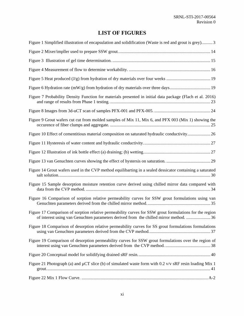
LIST OF FIGURES
Figure 1 Simplified illustration of encapsulation and solidification (Waste is red and grout is grey). ......... 3
Figure 2 Mixer/impller used to prepare SSW grout. ................................................................................... 14
Figure 3 Illustration of gel time determination. ......................................................................................... 15
Figure 4 Measurement of flow to determine workability. .......................................................................... 16
Figure 5 Heat produced (J/g) from hydration of dry materials over four weeks ........................................ 19
Figure 6 Hydration rate (mW/g) from hydration of dry materials over three days ..................................... 19
Figure 7 Probability Density Function for materials presented in initial data package (Flach et al. 2016) and range of results from Phase 1 testing. ........................................................................................... 23
Figure 8 Images from 3d-uCT scan of samples PFX-001 and PFX-005. ................................................... 24
Figure 9 Grout wafers cut cut from molded samples of Mix 11, Mix 6, and PFX 003 (Mix 1) showing the occurence of fiber clumps and aggregate. ........................................................................................... 25
Figure 10 Effect of cementitious material composition on saturated hydraulic conductivity. .................... 26
Figure 11 Hysteresis of water content and hydraulic conductivity. ............................................................ 27
Figure 12 Illustration of ink bottle effect (a) draining; (b) wetting. ............................................................ 27
Figure 13 van Genuchten curves showing the effect of hystersis on saturation. ........................................ 29
Figure 14 Grout wafers used in the CVP method equilibarting in a sealed dessicator containing a saturated salt solution. ......................................................................................................................................... 30
Figure 15 Sample desorption moisture retention curve derived using chilled mirror data compared with data from the CVP method. ................................................................................................................. 34
Figure 16 Comparison of sorption relative permeability curves for SSW grout formulations using van Genuchten parameters derived from the chilled mirror method. ......................................................... 35
Figure 17 Comparison of sorption relative permeability curves for SSW grout formulations for the region of interest using van Genuchten parameters derived from the chilled mirror method. ...................... 36
Figure 18 Comparison of desorption relative permeability curves for SS grout formulations formulations using van Genuchten parameters derived from the CVP method. ....................................................... 37
Figure 19 Comparison of desorption permeability curves for SSW grout formulations over the region of interest using van Genuchten parameters derived from the CVP method. ......................................... 38
Figure 20 Conceptual model for solidifying drained sRF resin. ................................................................. 40
Figure 21 Photograph (a) and µCT slice (b) of simulated waste form with 0.2 v/v sRF resin loading Mix 1 grout. .................................................................................................................................................... 41
Figure 22 Mix 1 Flow Curve. ................................................................................................................... A-2
SRNL-STI-2017-00564 Revision 0
xii
Figure 23 Mix 1a Flow Curve. .................................................................................................................. A-2
Figure 24 Mix 2 Flow Curve. ................................................................................................................... A-3
Figure 25 Mix 3 Flow Curve. ................................................................................................................... A-3
Figure 26 Mix 4 Flow Curve. ................................................................................................................... A-4
Figure 27 Mix 6 Flow Curve. ................................................................................................................... A-4
Figure 28 Mix 6a Flow Curve. .................................................................................................................. A-5
Figure 29 Mix 8 Flow Curve. ................................................................................................................... A-5
Figure 30 Mix 10 Flow Curve. ................................................................................................................. A-6
Figure 31 Mix 11 Flow Curve. ................................................................................................................. A-6
Figure 32 Mix 13 Flow Curve. ................................................................................................................. A-7
Figure 33 Mix 13a Flow Curve. ................................................................................................................ A-7
Figure 34 Characteristic Curves for Solid Secondary Waste Mix PFX-003 – Measured Vapor Pressure D-2
Figure 35 Characteristic Curves for Solid Secondary Waste Mix PFX-005 – Measured Vapor Pressure D-2
Figure 36 Characteristic Curves for Solid Secondary Waste Mix PFX– Measured Vapor Pressure ........ D-3
Figure 37 Characteristic Curves for Solid Secondary Waste Mix 1 – Measured Vapor Pressure ............ D-3
Figure 38 Characteristic Curves for Solid Secondary Waste Mix 1R – Measured Vapor Pressure ......... D-4
Figure 39 Characteristic Curves for Solid Secondary Waste Mix 1a – Measured Vapor Pressure .......... D-4
Figure 40 Characteristic Curves for Solid Secondary Waste Mix 2 – Measured Vapor Pressure ............ D-5
Figure 41 Characteristic Curves for Solid Secondary Waste Mix 3 – Measured Vapor Pressure ............ D-5
Figure 42 Characteristic Curves for Solid Secondary Waste Mix 5 – Measured Vapor Pressure ............ D-6
Figure 43 Characteristic Curves for Solid Secondary Waste Mix 6 – Measured Vapor Pressure ............ D-6
Figure 44 Characteristic Curves for Solid Secondary Waste Mix 6a – Measured Vapor Pressure .......... D-7
Figure 45 Characteristic Curves for Solid Secondary Waste Mix 8 – Measured Vapor Pressure ............ D-7
Figure 46 Characteristic Curves for Solid Secondary Waste Mix 10 – Measured Vapor Pressure .......... D-8
Figure 47 Characteristic Curves for Solid Secondary Waste Mix 10R – Measured Vapor Pressure ....... D-8
Figure 48 Characteristic Curves for Solid Secondary Waste Mix 11 – Measured Vapor Pressure .......... D-9
Figure 49 Characteristic Curves for Solid Secondary Waste Mix 12 – Measured Vapor Pressure .......... D-9
Figure 50 Characteristic Curves for Solid Secondary Mix 13 – Measured Vapor Pressure ................... D-10

SRNL-STI-2017-00564 Revision 0
xiii
Figure 51 Characteristic Curves for Solid Secondary Mix 13 – Measured Vapor Pressure ................... D-10
Figure 52 Characteristic Curves for Solid Secondary Mix 1 – Controlled Vapor Pressure ...................... E-1
Figure 53 Characteristic Curves for Solid Secondary Mix 1a – Controlled Vapor Pressure .................... E-1
Figure 54 Characteristic Curves for Solid Secondary Mix 2 – Controlled Vapor Pressure ...................... E-2
Figure 55 Characteristic Curves for Solid Secondary Mix 3 – Controlled Vapor Pressure ...................... E-2
Figure 56 Characteristic Curves for Solid Secondary Mix 5 – Controlled Vapor Pressure ...................... E-3
Figure 57 Characteristic Curves for Solid Secondary Mix 6 – Controlled Vapor Pressure ...................... E-3
Figure 58 Characteristic Curves for Solid Secondary Mix 6a – Controlled Vapor Pressure .................... E-4
Figure 59 Characteristic Curves for Solid Secondary Mix 8 – Controlled Vapor Pressure ...................... E-4
Figure 60 Characteristic Curves for Solid Secondary Mix 10 – Controlled Vapor Pressure .................... E-5
Figure 61 Characteristic Curves for Solid Secondary Mix 11 – Controlled Vapor Pressure .................... E-5
Figure 62 Characteristic Curves for Solid Secondary Mix 12 – Controlled Vapor Pressure .................... E-6
Figure 63 Characteristic Curves for Solid Secondary Mix 13 – Controlled Vapor Pressure .................... E-6
Figure 64 Characteristic Curves for Solid Secondary Mix 13a – Controlled Vapor Pressure .................. E-7
Figure 65 Characteristic Curves for Solid Secondary Mix PFX-004 – Controlled Vapor Pressure ......... E-7
Figure 66 Characteristic Curves for Solid Secondary Mix PFX-006 – Controlled Vapor Pressure ......... E-8

SRNL-STI-2017-00564 Revision 0
xiv
LIST OF ACRONYMNS
3d-μCT Three Dimensional Micro Computed Tomography BFS Blast Furnace Slag CM Cementitious Material COPC Constituent of Potential Concern CVP Controlled Vapor Pressure DAS Disposal Authorization Statement DM Dry Mix DOE Department of Energy ETF Effluent Treatment Facility FA Fly Ash FFTF Fast Flux Test Facility FY Fiscal Year HEPA High-Efficiency Particulate Air HIC High Integrity Container HLW High-Level Waste IDF Integrated Disposal Facility ILAW Immobilized low-activity waste ITZ Interfacial Transition Zone IXr Ion exchange resin Kd Distribution coefficient LAW Low-Activity Waste LDR Land Disposal Restrictions LFRG Low-Level Waste Disposal Facility Federal Review Group LLW Low-level waste MLLW Mixed Low-level Waste n/a Not applicable OPC Ordinary Portland Cement PA Performance Assessment PDF Probability Distribution Function Sd Sand sRF Spherical Rescorcinal Formaldehyde SRNL Savannah River National Laboratory SSW Solid Secondary Waste UPV Ultra-sonic Pulse Velocity v/v Volume/volume WAC Waste Acceptance Criteria WRPS Washington River Protection Solutions WTP Waste Treatment and Immobilization Plant

SRNL-STI-2017-00564 Revision 0
1
1.0 Introduction The Waste Treatment and Immobilization Plant (WTP) at Hanford is being constructed to treat 56 million gallons of radioactive waste currently stored in underground tanks at the Hanford site. This treatment includes vitrification of high-level waste (HLW) and low activity waste (LAW) fractions. Operation of the Vitrification facilities will generate several solid secondary waste (SSW) streams including used process equipment, contaminated tools and instruments, decontamination wastes, high-efficiency particulate air filters (HEPA), carbon adsorption beds, Ag-mordenite iodine sorbent beds, and spent ion exchange resins (IXr). All of which are to be disposed in the Integrated Disposal Facility (IDF). Washington River Protection Solutions, LLC (WRPS) requested the Savannah River National Laboratory (SRNL) support development of waste form formulations and testing specific to performance requirements and characteristics of SSW expected to be generated during the Hanford tank waste treatment mission (Brown, 2016). The Statement of Work (Requisition #281842 Revision 1) included testing of a variety of potential formulations for grouts being considered for encapsulation of debris waste and stabilization/solidification of non-debris waste. Results from this project include waste form-specific material properties for use as part of the IDF PA maintenance activities and recommendations for formulations and disposal options for SSW.
1.1 Purpose of this Report This project is addressing four key SSW streams. The four waste streams and assumed management approaches are summarized below. Testing in FY 2017 addressed properties of the neat grout formulations and waste forms with IXr mixed into selected grout formulations. Chapters 1 – 3 provide background information on the assumed waste disposal configurations, integration of the testing program with the IDF PA maintenance process, and the general approach for the testing program. The balance of the report describes the tests and results obtained. Chapter 2 describes the integration of this project with the IDF PA maintenance process. The general test program is then described in Chapter 3 followed by a discussion of the test results in the balance of the main report. The recognized limitations of the 2016 SSW data package (Flach et al., 2016) and the results of the IDF PA, together, formed the basis for the testing priorities for this project. The intent was to begin with testing to obtain basic information to confirm the hydraulic properties assumed for the IDF PA. This allowed time for initial PA calculations to be conducted to identify specific Constituents of Potential Concern (COPCs) on which to initially focus to confirm assumptions for chemical properties (e.g., Kds and diffusion coefficients). SRNL prepared samples to develop experimentally determined parameters for different grout formulations and waste forms to support waste form development and qualification and confirm assumptions used for the 2017 IDF PA. Development and testing of these samples conducted from October 2016 to June 2017 is documented in this report. Plans for testing during the remainder of FY 2017 are also summarized. The test results for key PA inputs are compared to the recommendations from the data package prepared in 2016 to assess the continued validity of the initial PA assumptions.
1.2 Key Solid Secondary Waste Streams The SSW streams being considered for the 2017 IDF Performance Assessment (PA) are described in detail in the IDF PA inventory data package, RPP-ENV-58562 (Prindiville, 2016). Four specific SSW streams were identified by the IDF PA team for detailed consideration in this project: Granular Activated Carbon (carbon adsorber beds), IXr, HEPA Filters, and silver-mordenite. Details regarding the ranges of inventories of key contaminants of potential concern in each waste stream and the volumes of waste are

SRNL-STI-2017-00564 Revision 0
2
provided in the IDF PA inventory data package. Descriptions from the inventory data package for each of these key waste streams are briefly summarized here followed by a brief description of the assumed final waste forms.
1.2.1 Carbon adsorber beds SSW inventory data from the Hanford Tank Waste Operations Simulator shows that the LAW Melter spent adsorber beds and Ag-mordenite (see below) are major contributors of I-129. The carbon adsorber beds are part of the LAW off-gas treatment system and contain activated carbon for mercury and halide (Hg, F) removal as well as I-129 abatement. Carbon adsorber beds are considered non-debris mixed low level waste (MLLW), which from a treatment perspective, contain potentially problematic amounts of Hg and I-129. Although treatment may remove some of the hazard, the conservative recommendation for disposition of this waste is to dispose of it at IDF. The beds would be transported to a local offsite treatment facility where they would be repackaged into suitable disposal containers with a stabilization grout for Resource Conservation and Recovery Act (RCRA) metals and Hanford Category 3 radioactive waste containment using a Hanford approved grout formulation that meets regulatory criteria.
1.2.2 Ion exchange resin Ion exchange resins and HEPA filters (see next section) are the largest sources of Tc-99 for SSW. After being dewatered, the IXr (Hanford Category 3 non-debris MLLW) would be transported offsite for treatment. At the treatment facility, the resin would be blended with a Hanford approved stabilization grout and placed in an container to meet requirements for RCRA metals and Hanford Category 3 radioactive waste containment using a Hanford approved grout formulation meeting regulatory criteria.
1.2.3 HEPA filters The current assumption is that non-woven glass paper (borosilicate microfiber) HEPA filters would be used. The filters could be either MLLW or LLW debris depending on their location and function within the WTP facility. All HEPA filters (both Category 1 and Category 3) are expected to be sent to an offsite treatment facility in carbon steel 55-gallon drums where they will be compacted into “pucks” at an approximated compaction ratio ranging from 5:1 to 10:1. Multiple pucks would be placed into suitable disposal boxes and macroencapsulated with grout to meet Land Disposal Restriction (LDR) requirements for RCRA constituents 1 . This macroencapsulation process would meet Category 3 stabilization requirements, which exceeds Category 1 requirements making this latter categorization irrelevant.
1.2.4 Ag-mordenite cartridges Silver impregnated adsorbers (e.g., Ag-mordenite) are designed to capture iodine from off gas systems, and thus, similar to the carbon adsorbers can be one of the primary sources of iodine in the IDF inventory. The Ag-mordenite waste stream is expected to be non-debris MLLW similar to the carbon adsorber beds, and may include problematic concentrations of Hg and 129I. Although treatment may remove some of the hazard, the conservative recommendation at this time is to assume disposal at IDF without removal of COPC. The Ag-mordenite would be transported to a local offsite treatment facility where they would be repackaged into suitable disposal containers blended with a stabilization grout for RCRA metals and Hanford Category 3 radioactive waste containment using a Hanford approved grout formulation that meets regulatory criteria.
1 The work authorization process implemented at the treatment facility determines the allowable number of pucks based on waste stream characterization information provided by the waste generator at the time of shipment to the treatment facility. Disposal box limits (after drums are compacted into pucks at a compaction ratio of approximately 10:1) are closely managed such that Category 3 limits are not exceeded.

SRNL-STI-2017-00564 Revision 0
3
1.3 Conceptual Waste Forms SSW is classified into two categories: debris waste (defined in Washington Administrative Code section 173-303-040 as waste with a particle size greater than 60 mm) and non-debris waste (waste with a particle size less than or equal to 60 mm). For the purposes of this report, the terms solidification (also referred to as stabilization) and encapsulation (also referred to as macroencapsulation) are used to represent two basic configuration of the disposed waste, see Figure 1. From the perspective of input data for the PA, material properties for the final waste form using a generally applicable formulation can be identified for the encapsulating media, because it is not mixed with the waste stream. For a stabilized waste stream, the input data may depend to some extent on the specific waste mixed with the grout.
Figure 1 Simplified illustration of encapsulation and solidification (Waste is red and grout is grey).
Solidification represents the case where a solid waste less than 60 mm in diameter is intimately blended with the cementitious material (i.e., waste is more or less evenly distributed throughout the waste form). In this case the properties of the waste form will represent the integrated mixture of waste and solidification media. Encapsulation assumes a specified minimum thickness of clean encapsulating media completely surrounding the waste. Although this is not the disposal approach identified in the inventory report, there is the potential for non-debris waste to be “encapsulated” into a container made of cementitious or other materials. The necessary thickness of the encapsulating media around the waste would be determined in an iterative manner based on results of the PA.
1.4 Assumed SSW Forms A baseline for waste forms was established in the Inventory Data Package for the IDF PA (Prindiville, 2016). It is expected that a standard grout formulation would be used. The exact formulation is still being investigated but mixtures containing water, ordinary portland cement (OPC), blast furnace slag (BFS), fly ash (FA), and/or aggregate are being considered.
1.4.1 Proposed Waste Forms Compacted HEPA filters are considered as MLLW debris requiring macroencapsulation and the other three key waste streams (carbon absorption beds, silver mordenite iodine sorbent beds, and spent IXr) were assumed to be non-debris mixed LLW requiring solidification/stabilization (Prindiville, 2016). Although this assumption was used as the baseline, it was recommended in the SSW data package (Flach et al., 2016) to also explore the option of directly disposing SSW streams in containers or the option of

SRNL-STI-2017-00564 Revision 0
4
encapsulating spent IXr, activated carbon and silver mordenite with a layer of clean grout, similar to macroencapsulation of the HEPA filters. Radioactive LLW IXr that are not considered hazardous waste are often disposed in high integrity containers without stabilization. Flach et al. (2016) and others have identified the possibility for waste forms specifically designed to retain certain contaminants (resins, activated carbon, silver mordenite) to not perform as well for long-term releases, if mixed with a cementitious material. Thus, it may be advantageous in the context of long-term release rates to not mix them in a grout. DOE has formally notified the Washington Department of Ecology about alternatives for treatment and disposal of SSW (Smith, 2015). One notable difference from the above assumptions is the letter indicates that macroencapsulation is the treatment option for silver mordenite. HEPA filters were the current drivers in preliminary PA calculations, thus properties of the macroencapsulation media are considered a priority to confirm. Initial testing focused on potential macroencapsulation grout mixes. Current practices for MLLW debris disposal at the Hanford site have been selected as the baseline for SSW management. MLLW debris disposed of in Hanford’s 200 West Area Burial Ground is placed in a carbon steel standard waste box (B25) and encapsulated with a grout commonly referred to as Hanford Mix 5, also referred to as American Rock Products 4257020-Perma Fix Grout 2500 PSI [0]. The grout is mixed at a batch plant and transported via concrete truck (transit mixer) to the Perma-Fix facility where it is poured into a B25 box containing debris. The grout cures in the B25 uncovered for ~72 hours prior to being covered and transported to the Hanford 200 West Area Low Level Waste Burial Ground for disposal. If bleed water is detected at the end of the 72 hour holding period, diatomaceous earth is added to the surface of the grout to sorb the free liquid prior to being covered. Ventilation is the only environmental control for the process and the storage room. No fresh properties are measured during batching or placement of the grout and there are no technical requirements for the fresh or cured grout, except for the compressive strength. Hanford Mix 5 is also assumed as the baseline for solidification/stabilization of non-debris SSW.
1.4.2 Other Example Waste Forms The initial testing program has focused on the baseline plans for waste forms that would be used for disposal at IDF based on current practices at Hanford. However, alternative waste forms are also being identified as part of this project for consideration depending on properties obtained for the baseline. Seitz (2017) includes a variety of examples of waste forms that have been used for SSW. A report by Different by Design (Kay et al., 2017) also includes a detailed description of waste management practices in the United Kingdom with some examples from other countries as well.

SRNL-STI-2017-00564 Revision 0
5
2.0 Integration with IDF PA Maintenance DOE Manual 435.1-1, Radioactive Waste Management Manual includes a requirement to maintain a PA and Disposal Authorization Statement (DAS) for a disposal facility. The maintenance process can address a number of areas, for example: research to address outstanding issues raised by a Low-Level Waste Disposal Facility Federal Review Group PA review team; changes in waste forms, design, operations, etc. that were not addressed in the PA; and new field data or unexpected monitoring data. Specific application of the maintenance process for the IDF PA is described in this chapter.
2.1 General Approach for Maintenance Hundreds of potential inputs need to be considered for a PA. It is not realistic or efficient to assume that extensive efforts are needed to seek detailed data for every input parameter for the PA. For SSW for the IDF PA, there is close coordination to integrate the data collection efforts with the team conducting the PA to establish priorities for specific data collection efforts. The approach for the IDF PA started by identifying necessary modeling inputs and providing recommendations for input values and distributions (where possible) based on existing information. This was documented in the 2016 data package for SSW described in Flach et al. (2016). In the case of SSW for the IDF PA, there is a recognized need to obtain formulation and waste form specific information to confirm assumptions in the initial data package. The baseline grout mix currently used for encapsulation of SSW at Hanford had not been tested to obtain the data required for the IDF PA. The specifications for the grout that will be used for SSW have also not been identified, so there is a need to provide data for a baseline and some alternative grout mixes. For example, it is uncertain whether it will be necessary to include BFS in a mix to address potential Tc-99 releases, so alternative mixes containing BFS are being tested in addition to a baseline mix based on the formulation currently used at Hanford. Practical considerations are also influencing the testing program. The testing program is designed to consider ranges in the mix ratios to identify the influence on the measured properties. If the testing can show minimal changes in key properties across a range of mix ratios, then it will provide flexibility for operations to not require extreme controls on the process. Similarly, resin testing is considering a range of resin loading and water to cement ratios for the waste forms with the intent to support flexibility for the specifications used for solidifying/stabilizing resins.
2.2 Initial Data Package (2016) The 2016 SSW data package provided recommendations for waste form physical and chemical properties for use as inputs for the initial analysis of disposal of SSW in the 2017 IDF PA. Specific formulations had not been identified for cementitious materials that will be used to encapsulate or solidify SSW, and no IDF-specific experiments were conducted to obtain SSW data for the PA. The data package focused on the four key SSW streams: HEPA filters, ion exchange resins, carbon adsorber beds and Ag-mordenite. The IDF PA team identified specific COPCs expected to be the key contributors for the PA calculations: 99Tc, 129I, 137Cs, 90Sr, uranium isotopes (and total uranium), chromium, mercury, and nitrate. Those species were addressed in the data package to support the PA. The data package includes recommended inputs for the physical properties of the cured cementitious materials (e.g., saturated hydraulic conductivity, bulk density, porosity, moisture characteristic curves), assumptions governing the release of contaminants of concern from the key waste streams, and properties associated with mass transport of the contaminants of concern through the cured cementitious materials (e.g., distribution coefficients, solubility, diffusion coefficients). There were differing amounts of information available for specific input parameters for existing mix designs. Collectively, the recommendations are representative of the available data.

SRNL-STI-2017-00564 Revision 0
6
A combination of distributions and recommended values, including uncertainty regarding the mix formulations, were provided to give inputs in a form that facilitated the development and implementation of the uncertainty and sensitivity analysis tools for the 2017 IDF PA. Sensitivity and uncertainty analyses based on these initial recommendations were used to gain insights into assumptions and uncertainties that are significant for the conclusions of the PA. This, in turn, provided the ability to identify the range of acceptable conditions and also identify critical areas where refined, mix- and waste form-specific, information was needed as part of PA maintenance. These insights were used to guide the selection of mixes and prioritize the needs for specific laboratory studies. Initial modeling using this representative data was also used to identify less sensitive parameters for which further study may be less important and specifications for mixes and waste forms can be expressed as ranges to be more flexible, which will be expected to be beneficial for operations
2.3 Basis for Current Testing The recognized limitations of the 2016 data package and the results of the IDF PA, together, formed the basis for the testing priorities for this project. The intent was to begin with testing to obtain basic information to confirm the hydraulic properties assumed for the IDF PA. This allowed time for initial PA calculations to be conducted to identify specific COPCs on which to initially focus to confirm assumptions for chemical properties (e.g., Kds and diffusion coefficients).
2.3.1 Limitations of 2016 Data Package Development of the testing program began from the perspective of confirming waste form specific information relative to the assumed properties provided in the data package. The highest priorities included confirming the physical and chemical (e.g., Kd) properties of Hanford Grout Mix 5 and confirming physical properties of the blended grout and resin waste form. The hydraulic properties for this blended waste form were assumed to be like a mortar (mix of cement and small aggregate) as a starting point. There was uncertainty about how representative that assumption would be, which led to higher priority for testing. The geochemical properties included in the 2016 data package were also estimated based on literature data. It was expected that many of the assumed ranges of values may not have a significant influence on the conclusions of the PA, but it was anticipated that some testing would be needed to confirm any values identified as potentially significant for PA conclusions.
2.3.2 Current IDF PA Results The IDF PA is currently in draft form and is planned for submittal to the Low-Level Waste Disposal Facility Federal Review Group at the end of September 2017. Preliminary results have been discussed with the IDF PA team and some general trends have been observed. SSW is the most significant contributor to groundwater concentrations and the peak doses in the base case. Specifically, 129I and 99Tc associated with HEPA filters have the greatest contribution to the peak dose. Thus, assumptions regarding encapsulation media and performance of the HEPA filter waste form should be a focus of attention. Several assumptions are made that influence releases from the HEPA filters. Uncertainties that affect the ability to retain 129I and 99Tc in the HEPA filter encapsulated waste forms include: (1) the sorption properties for 129I and 99Tc on the HEPA filters, (2) the hydraulic, diffusive and transport properties of the encapsulating grout, (3) the representativeness of laboratory-derived properties to the scale of the containers planned for use, (4) the impact of operational factors (curing, handling, transportation, storage) on the hydraulic, diffusive and transport properties and geometry (i.e., thickness) of the as-cured grouted waste form, and (5) the effect of grout penetrating the compacted debris waste on the hydraulic, diffusive and transport properties of the waste form. Confirmatory testing is already underway to address hydraulic

SRNL-STI-2017-00564 Revision 0
7
properties and sorption properties of the encapsulation grout. Hydraulic and physical testing information for some grout compositions are provided in this report. Additional areas where uncertainties in preliminary results can have an impact include assumptions about the performance of other SSW forms. Hydraulic properties assumed for non-debris waste forms that are blended with grout can potentially influence results, if the waste forms do not perform as well as assumed. Similarly, if assumptions about the sorptive properties of activated carbon and silver mordenite are negatively impacted by mixing with grout and outside the range assumed for the IDF PA, there is potential for an increase in the release rate from these wastes that could influence conclusions of the PA. These are additional areas where confirmatory testing is expected.

SRNL-STI-2017-00564 Revision 0
8
3.0 General Approach for SSW Testing Program Waste form testing to support the IDF PA is being conducted to address 3 different goals:
1. Evaluate Grout Options for Waste Forms 2. Test Waste Forms – Physical and Hydraulic Performance 3. Test Waste Forms – Chemical Performance
These three goals are being addressed incrementally with each phase of the testing building on results from the previous set of tests and considering new information from the IDF PA calculations. Each phase, as the testing becomes more complex, is intended to become more focused on a limited set of mixes and on key considerations for the IDF PA. For FY17, three phases were identified:
• Phase 1 – Hydraulic and Physical Testing of Potential Neat Grout Mixes • Phase 2 – Down Select from Mixes Considered in Phase 1
o Part 1 – Hydraulic and Physical Testing of Ion-Exchange Resins Blended with Grout o Part 2 – Kd Testing of Neat Grout
• Phase 3 – Testing of Releases of Key COPCs from Waste Forms The first phase starts broad addressing a variety of potential combinations of dry materials and moisture contents. Options for mixes are then down selected for consideration in more specific waste form and Kd testing with neat grout in Phase 2. The initial emphasis of waste form testing addresses ion exchange resins and HEPA filters in order to first confirm physical and hydraulic properties of a neat grout and grout blended with a non-debris waste form. Resins were specifically selected as a priority because of the potential for volume change and uncertainties regarding impacts on hydraulic and physical properties. Similar to the neat grout testing, adjustments to the mix designs were also considered during fresh property testing of the resin blended with grout, especially to consider the amount of residual moisture present in the resins before mixing with the grout. Phase 3 is expected to address, prioritized based on PA results, releases of key COPCs from resins and other waste forms that are deemed most significant in the PA.
3.1 2017 Test Plans Detailed plans for the SSW testing program are described in the Technical Task and Quality Assurance Plan for Hanford Solid Secondary Waste Formulation Development and Waste Form Qualification (Nichols and Kaplan, 2017). A summary of the activities conducted and plans is provided below. Note that the second part of Phase 2, as implemented, is a deviation from the original plan. The original plan included a proposed demonstration of macroencapsulation of compacted, clean HEPA filters at the drum scale and then cutting the drum and waste form for a visual examination of the effectiveness of the macroencapsulation. Based on feedback from the IDF PA team and DOE, this was modified to accelerate efforts to address the distribution coefficients for key COPCs in encapsulation grouts selected from Phase 1, which was deemed to be a higher priority based on early PA results.
3.2 Phase 1: Encapsulation Grout Hydraulic and Physical Properties The first phase of testing involved evaluating a variety of neat grout mixes designed around the baseline formulations that have a history of use at Hanford. One mix that is being used at the Savannah River Site was also included. Variations in moisture and dry materials percentages were considered during the first stage. This phase is an exploratory phase to evaluate options for grout to be used in waste form

SRNL-STI-2017-00564 Revision 0
9
development. Fresh and cured physical and hydraulic properties were evaluated to compare with the 2016 data package and support decisions to down-select from the range of mix options from Phase 1 to a few preferred options that are carried forward for waste form specific testing and evaluations of chemical performance.
Table 1 Fresh and cured properties to be measured in Phase 1.
Property Comments Fresh Properties
Gel Time Screening test for flowability and indication of how long after an interruption of the process it can be resumed before it is necessary to clean-up and re-start.
Grout Flow Property related to workability i.e. and how well a grout would flow around objects when used for encapsulation, self leveling.
Rheology Property used to determine whether a grout can be pumped and in the design of pumping systems.
Heat of Hydration Gauge the onset and extent of hydration reactions and maintain temperature limits as the waste form cures
Density Used in pump design Set Time Used to assess when a concrete
has hardened sufficiently and is no longer deformable.
Free Liquids Also referred to as bleed, is an indication of settlement of heavier cementitious material
Cured Properties Density Input for transport calculations in
Performance Assessment. Porosity Input for transport calculations in
Performance Assessment. Compressive Strength Used to ensure waste form will
survive forces from transportation and disposal.
Saturated Hydraulic Conductivity Input for flow calculations in Performance Assessment.
Moisture Retention Input for flow calculations in Performance Assessment.
3.3 Phase 2 – Part 1: Resin in Grout A subset of formulations selected in the exploratory testing of cementitious materials is being used for Phase 2 testing. Part 1 of Phase 2 focuses on physical and hydraulic performance of spherical Rescorcinol Formaldehyde (sRF) ion exchange resin waste forms. Waste forms were prepared by

SRNL-STI-2017-00564 Revision 0
10
blending clean sRF ion exchange resins using grout formulations down selected from exploratory testing in Phase 1. H+ form sRF resins have a density ranging from 0.36-0.46 g/mL. Maintaining entrainment of sRF in thin grouts such as Hanford Grout #5 dry materials prior to setting was a practical concern considered during the initial preparation of samples. The first set of samples prepared in this phase were quantitatively analyzed for fresh properties and qualitatively analyzed to assess integration of the ion exchange resins into the cementitious material and to explore evidence of changes in resin volume. Fresh property testing was used to evaluate the impact of the relatively large amount of added residual water in the sRF resins to the grout mixes that also include water and consider the need to modify mixes. Three different types of other inspections are also being conducted: visual inspection of a cut sample, imaging with three dimensional micro x-ray computed tomography (3d-μCT) and optical scanning electron microscopy. Samples are also being tested to determine cured hydraulic and physical properties similar to Phase 1 to confirm assumption from the 2016 data package. Performance testing of sRF resin is also underway for the Test Specification for the Low-Activity Waste Pretreatment System Full-Scale Ion Exchange Column Test and Engineering-Scale Integrated Test (Project T5L01) (WRPS, 2016). Spent material from the full-scale sRF resin testing is being collected for use in this study as it would closely resemble spent sRF resin that is expected to be disposed of as SSW in the IDF. Information from physical and hydraulic performance testing for sRF resin will be used to identify grout mixes and waste loading that should be carried forward for testing using wastes containing COPCs or appropriate surrogates.
3.4 Phase 2 – Part 2: Distribution Coefficients for Encapsulation Grout A subset of the mixes from Phase 1 are also being used for sorption testing of the neat grout mixes to confirm assumptions for Kds that were identified in the 2016 data package. Kds are not currently available for Hanford Mix 5. The neat grout mixes, including Hanford Mix 5, are representative of encapsulation grouts that could be used for HEPA filters. Assumptions for Kds in the encapsulation grout are an important input in the IDF PA given the significance of the HEPA filters in initial PA results. The initial sorption tests involve spiking a solution with selected COPCs and mixing it with crushed grout to evaluate the ratio of COPC that remains in solution with the amount that reacts with the grout, which is representative of contaminated pore solution from HEPA filters migrating into the encapsulation grout. As previously mentioned the debris and non-debris waste for IDF is expected to include cation, anion, radioactive and hazardous COPCs. These COPCs exhibit a wide range of behavior depending on the chemical environment they are in. These tests will be conducted under a range of management scenarios to simulate different geochemical conditions that may be encountered during the expected lifetime of the IDF (i.e., pH and redox).
3.5 Phase 3 – Part 1: Spiked Waste Form Plans are currently being developed for testing of spiked waste forms for Phase 3. The first waste form will likely be ion exchange resins blended in a selected grout mix. Specifics regarding which COPCs and how the COPCs will be introduced into the waste form are being developed at this time. Tests being considered include: diffusion coefficients and Kds. Waste form specific Kds and diffusion coefficients are not available for resin and other non-debris mixed with Hanford Mix 5 and the other alternatives being considered. Current PA assumptions are based on available information that needs to be confirmed based on the actual waste and proposed grout mixes.

SRNL-STI-2017-00564 Revision 0
11
Other potential testing being considered for FY 2018 includes testing of HEPA filters (or representative media) spiked with COPCs and encapsulated in neat grout and/or testing of granular activated carbon or silver mordenite to evaluate potential impacts of grout on releases from those waste forms.

SRNL-STI-2017-00564 Revision 0
12
4.0 Phase 1 Methods and Results Phase 1 testing was an exploratory phase to become familiar with the materials used in the baseline grout (Hanford Grout Mix 5) for the IDF PA and to begin building a dataset of properties to compare with assumptions in the 2016 data package for the IDF PA. Several variations of the baseline grout recipe were selected to determine properties of grouts with different geochemical properties that may perform better retaining contaminants that are anticipated to be in the waste that will be grouted. Specifically, BFS, content, FA:OPC ratio and water to H2O:cementitious materials (CM) ratio H2O:CM.
4.1 Sample Preparation Grout batches were prepared using ASTM C-150 Type I-II cement (OPC), BFS, Class F fly ash, sand (SD), admix BASF Pozzolith 80 and BASF Master Fiber M100 single monofilament polypropylene fibers from samples provided by American Rock Products, Lafarge Northwest, and BASF. The elemental composition of the cementitious materials used in this study was determined using x-ray fluorescence, results are presented in Table 2. A list of the mixes considered for Phase 1 is provided in Table 3. Grouts were prepared by adding dry mix (DM) CM and aggregate (when applicable) to a beaker containing water that was being stirred by an overhead mixer. Mixer speed was adjusted to maintain a vortex in the grout as DM was added. Once all of the DM was in the admix the fiber was added. Fiber was shredded by hand using tweezers to breakup up the fiber into smaller assemblages prior to adding it to the grout. After all ingredients were in the grout, the grout was stirred an additional five minutes ensuring there was a vortex at all times. Occasionally the mixer was stopped to “burp” the grout by removing air pockets that affect mixing. Once the mixing was complete the grout was immediately decanted for fresh property testing and into molds to cure.
Table 2 Composition of cementitious materials used in grout.
Element Cement Flyash Blast
Furnace Slag
CaO, wt% 63.9 13.0 41.2 SiO2, wt% 20.1 48.4 32.4
Al2O3, wt% 4.9 17.9 14.6
Fe2O3, wt% 3.3 6.5 0.8
SO3, wt% 3.1 0.6 2.5 MgO, wt% 0.9 5.4 5.3 K2O, wt% 0.3 1.7 0.3
TiO2, wt% 0.3 1.1 0.6
Na2O, wt% 0.3 3.7 0.2 SrO, wt% 0.1 0.3 0.1 P2O5, wt% 0.1 0.3 0.0
Mn2O3, wt% 0.0 0.09 0.2 LoI, wt% 2.6 0.8 1.9
Note: LoI = Material lost on ignition when preparing sample.

SRNL-STI-2017-00564 Revision 0
13
Table 3 List of mixes used in Phase 1 testing
Mix H2O:CM (w/w)
FA/OPC/BFS/SD (w/w) Comment
1 0.29 75/25/0/0 Current Hanford mix 5 used in burial ground 2 0.25 75/25/0/0 Prepared as intended 3 0.33 75/25/0/0 Prepared as intended 4 0.33 20/5/75/0 Abandoned due to low grout flow 5* 0.45 20/5/75/0 Replacement for Mix 4, increased H2O:CM to 0.45 6 0.33 45/30/25/0 Prepared as intended 7 0.25 45/30/25/0 Abandoned due to low grout flow 8 0.33 15/10/75/0 Abandoned due to low grout flow 9* 0.45 15/10/75/0 Replacement for Mix 8, increased H2O:CM to 0.45 10 0.33 60/15/25/0 Prepared as intended 11 0.25 60/15/25/0 Prepared as intended 12 0.41 14/14/0/72 Current Hanford mix 3 13 0.45 45/10/45/0 Cap material based on SRS saltstone
Phase 1 was implemented as follows based on the results of the flow testing:
• Mix 1-3, 6, and 10-13 prepared according to TTQAP • Mix 4 was too dry and did not meet the flow guideline of 120 mm. No further testing was
completed on Mix 4. • Mix 5* H2O:CM was increased to 0.45 because Mix 4 was too dry with 0.33 H2O:CM. A
H2O:CM of 0.45 was chosen to be consistent with Mix 13 which has a similar CM mix. • Mix 7 was too dry and did not meet flow guideline of 120 mm. No further testing was completed
on Mix 7 • Mix 8 was too dry and did not meet flow guideline of 120 mm. No further testing was completed
on Mix 8 • Mix 9* H2O:CM was increased to 0.45 because Mix 8 was too dry with 0.33 H2O:CM.

SRNL-STI-2017-00564 Revision 0
14
Figure 2 Mixer/impller used to prepare SSW grout.
4.2 Fresh Properties Fresh properties were measured immediately following preparation of grout batches. The fresh properties are generally not a direct input to the PA, but provide information regarding practical use of the different mixes that will be of value from an operational perspective. A summary of the fresh properties results is provided in Table 4. Each of the test results are briefly described in the following subsections.
Table 4 Fresh properties for mixes prepared in Phase 1
Mix Density (gm/mL)
Flow (mm)
UPV (cm/sec)
Vicat / Set Time (mm/hr)
Bleed 24 hr (gm)
Gel Time (mm:ss)
1 1.96 109 1490 0.0 / <24hr 0.0 5:25 2 2.02 115 2395 0.0 / <24hr 0.0 6:30 3 1.88 176 1508 0.0 / <24hr 0.0 5:00 4 n/a 105 n/a n/a n/a n/a 5 1.79 128 2252 2.0 / <24hr 0.5, 0.01 2:00 6 1.95 149 2105 0.0 / <24hr 0.0 4:00 7 n/a 109 n/a n/a n/a n/a 8 n/a 107 n/a n/a n/a n/a 9 1.81 135 1326 0.0 / <24hr 0.0 1:00
10 1.92 187 1950 0.0 / <24hr 0.1, 0.01 12:00 11 2.02 126 2127 0.0 / <24hr 0.0 2:00 12 2.13 141 2772 Nm 0.0 45:00 13 1.77 196 2597 Nm nm 25:00 1a 1.98 132 2771 0.0 / <24hr 0.0 5:00
13a 1.75 161 2047 0.0 / <24hr 0.7 25:00 6a 1.94 122 2407 0.0 / <24hr nm 1:00
1 After 72 hours

SRNL-STI-2017-00564 Revision 0
15
4.2.1 Gel Time Gel time is a subjective method of determining duration of grout flowability. In a continuous process, the gel time is an indication of the time after an interruption in the grout making process that is available to restart the process before it becomes necessary to perform a clean-up/shut down sequence. Gel time is also an indication of how long the placed grout (in a waste container) can maintain flowability. Gel time was measured by filling five ~100 ml containers with fresh grout. A timer was started as the first cylinder was filled. The cylinders are sequentially opened and tipped over a second container, each after an increasing amount of time. The grout is deemed gelled when the grout will no longer pour from a cylinder under its own weight. An example gel test is illustrated in Figure 3. In this example, the slurry poured from the first three cylinders when tipped into the second container. The slurry would not pour from the fourth container after resting for a period of 40 minutes after filling. Gel time is therefore approximately 40 minutes for this slurry (Cozzi et al., 2017). The results for the gel time tests, for each of the mixes processed, are shown in Table 4. Gel times measured for this set of mixes ranged from 5 minutes to greater than two hours.
Figure 3 Illustration of gel time determination.
4.2.2 Grout Flowability The flow test provides information regarding workability and was the first fresh property measured. The results were used to determine if the batch was suitable for continued testing. Flow was determined by placing a stainless steel cylinder of known size open on both ends on a stainless steel plate and filling it completely full. Once the cylinder was full it was quickly lifted straight up to release the grout onto the stainless steel plate forming a “pancake” as shown in Figure 4. The diameter and thickness of the pancake was then measured using a caliper. Grout with a flow ≥ 120mm was considered workable for this study. A flow of ≥ 120mm was selected based on measurements of the grout batches prepared using the baseline cementitious material mix, which is known to be acceptable for current applications at Hanford.

SRNL-STI-2017-00564 Revision 0
16
Figure 4 Measurement of flow to determine workability.
4.2.3 Rheology A method to assess the rheological properties of flowable grouts is to obtain a flow curve and is the 2nd measurement that is obtained from the sample. The flow curve used to assess the grouts in this task had a linear shear rate up ramp of 0 to 300 sec-1 in five minutes, ; a 30 second hold at 300 sec-1; and a linear shear rate down ramp of 300 to 0 sec-1 in five minutes. It is assumed that during the flow curve measurements in this task, chemical reactions that impact the structure do not affect the measurement. The flow curves are regressed using rheological models to determine the coefficient in the models. The most common rheological model used to describe the flow of concrete, mortars, and cement is the Bingham Plastic model, equation (1). An alternative rheological model, the Herschel Bulkley (equation 21), can better assess for the yield stress if the fluid has both a yield stress and behaves like a power law fluid. 𝝉𝝉 = 𝝉𝝉𝑩𝑩𝑩𝑩 + 𝜼𝜼∞�̇�𝜸 (1) 𝝉𝝉 = 𝝉𝝉𝑯𝑯𝑩𝑩 + 𝒂𝒂�̇�𝜸𝒏𝒏 (2) Where: 𝜏𝜏 = the measured stress (Pa) �̇�𝛾 = the applied shear rate (sec-1) 𝜏𝜏𝐵𝐵𝐵𝐵 = Bingham Plastic yield stress (Pa) 𝜂𝜂∞ = Plastic viscosity (Pa-sec) 𝜏𝜏𝐻𝐻𝐵𝐵 = Herschel Bulkley yield stress (Pa) 𝑎𝑎 = consistency index (Pa-secn-1) 𝑛𝑛 = flow index (unitless) The rheological results using the Bingham Plastic and Herschel Bulkley models are provided for both the up and down curves in Table 5. The Bingham Plastic results were regressed between 50 to 300 sec-1, due to an noticeable power law functionality below 50 sec-1 for a majority of the grouts, as observed in Appendix A. The Herschel Bulkley model was regressed for the entire range of shear rate. The difference between the up and down curve values is due the thixotropic nature of the mixes as observed

SRNL-STI-2017-00564 Revision 0
17
between the up and down curves shown in Appendix A. In almost all cases, the yield stress for the Bingham Plastic was lower for the down curve as compared to the up curve and the plastic viscosities typically higher for the down curve. For the Herschel Bulkley results, the down curve yield stress was greater than the up curve for almost all cases and is most likely due to the thixotropic nature of the grouts. Given the different results for yield stress, the most appropriate values would be those obtained from the Herschel Bulkley down curve. Mix 12 flow curve could not be measured; the sample over-torqued the rheometer within 15 seconds of starting the measurement. The flowcurve measurement from Mix 12 settled quickly due to the large quantity of sane used, causing the bob to over torque the rheometer. This clearly indicates that this mixture is not suitable for use in applications that require pumping. It is recommended that this mix, if deemed suitable based on the other properties, be quantified for rheology for completeness.
Table 5 Rheology results for mixes prepared in Phase 1
Mix
Bingham Plastic Herschel Bulkley
Up Curve Down Curve Up Curve Down Curve
𝝉𝝉𝑩𝑩𝑩𝑩 (Pa)
𝜼𝜼∞ (cP)
𝝉𝝉𝑩𝑩𝑩𝑩 (Pa)
𝜼𝜼∞ (cP)
𝝉𝝉𝑯𝑯𝑩𝑩 (Pa)
𝒂𝒂 (Pa-sn-1)
𝒏𝒏 unitless
𝝉𝝉𝑯𝑯𝑩𝑩 (Pa)
𝒂𝒂 (Pa-sn-1)
𝒏𝒏 unitless
1 66.7 179 39.8 256 -23.4A 36.79 0.236 8.7 4.61 0.547 1a 55.6 206 41.6 232 2.1 13.97 0.365 5.3 6.50 0.484 2 45.3 388 45.5 359 1.9 6.02 0.569 6.2 5.23 0.580 3 38.4 121 27.6 153 -3.2A 13.91 0.296 6.3 3.48 0.513
5* 44.7 215 34.6 243 11.8 6.52 0.467 8.8 3.56 0.577 6 47.4 303 42.7 316 7.6 6.36 0.524 9.5 4.59 0.578 6a 72.4 359 48.3 432 7.6 6.36 0.524 9.5 4.59 0.578 9* 59.0 206 33.8 285 -1.4A 19.45 0.315 11.2 2.63 0.647 10 22.9 171 21.5 167 6.3 2.15 0.600 6.3 1.53 0.649 11 59.1 633 41.8 648 8.6 5.84 0.647 15.9 2.41 0.789 13 19.6 62 13.7 78 2.3 4.79 0.347 5.6 1.10 0.582 13a 19.8 109 19.8 107 2.3 4.79 0.347 5.6 1.10 0.582
A – Regression resulted in a negative yield stress, indicating this material has no yield stress due to the curvature (thixotropic response most likely) of the data in the lower region of the flowcurve. Data should
be analyzed as a power law fluid.
4.2.4 Heat of Hydration The isothermal heat of hydration for the Cast Stone mixes was measured in accordance with ASTM (C 1679), Standard Method for Measuring Hydration Kinetics of Hydraulic Cementitious Mixtures Using Isothermal Calorimetry (ASTM, C 1679). This measurement is used to compare the hydration kinetics of salt solutions and dry mix blends. The composition of the cementitious materials as well as the composition and amount of additives can affect the magnitude and timing of hydration heat development.

SRNL-STI-2017-00564 Revision 0
18
In large pours, the energy (heat) produced can alter the mineralogy and microstructure developed in the waste form and influence cured properties. An eight-channel isothermal calorimeter (TAM Air, TA Instruments, Newcastle, DE) was used to collect the heat generation rate and total energy of each of the mixes. Each channel consists of a twin configuration with one side for the sample and the other side for the reference material. The reference channel was balanced with 20 g of quartz sand to approximate the heat capacity of the mixes. The isothermal calorimeter was maintained at 25°C for the entirety of the testing. The mix was transferred to the calorimeter and the test initiated. After 30 days the test was terminated. The total energy produced, normalized per gram of dry blend material was determined. The maximum generation rate (heat flow) and the elapsed time to attain this rate were also determined. The heat produced over 30 days and the maximum heat generation are shown in Table 6. Dry blend components (OPC/BFS/FA/SD) each participate in the hydration reaction to different extents. In the construction field, the fine aggregate sand is not considered in the water to cementitious material calculation. However, when the information is used to determine the heat of the mix generated, all of the dry materials are considered to account for the dilution (heat sink) properties of the sand.
Table 6 Calorimetry Data for Mixes Prepared
Mix H2O:CM (w/w)
FA/OPC/BFS/SD
(w/w)
Energy at 30 d
(J/g)
Time to Peak
Energy (hr)
Energy at Peak
(µW/g) 1a 0.29 75/25/0/0 189 15:49 1981 2 0.25 75/25/0/0 181 23:02 1215 3 0.33 75/25/0/0 202 18:01 1443
5* 0.45 20/5/75/0 202 17:49 1582 6a 0.33 45/30/25/0 225 20:45 1963 9* 0.45 15/10/75/0 131 18:37 2366 10 0.33 60/15/25/0 151 25:12 1534 11 0.25 60/15/25/0 151 39:15 982 12 0.41 14/14/0/72 50 11:21 616 13 0.45 45/10/45/0 135 20:43 2365
The majority of the energy produced during curing occurs within the first four weeks. Figure 5 shows the heat produced in J/g for the dry materials in each of the mixes. In water based systems, the heat generated is dominated by the hydration of cement. Blast furnace slag hydration is somewhat slower as it depends on the solubility of the excess portlandite, (Ca(OH)2, in the cement to raise the pH of the water and activate the slag. Mix 12, the mix that contains 72 wt% sand and reflects Hanford Mix 3, produced the lowest amount of energy for the mix. A second parameter of the heat of hydration is the rate at which enerfy is produced. As noted above, the reaction is dominated by the hydtation of the cement component and the contribution of blast furnace slag lags. Figure 6 shows the rate at which hydration occurs for the first three days of curing.

SRNL-STI-2017-00564 Revision 0
19
Figure 5 Heat produced (J/g) from hydration of dry materials over four weeks
Figure 6 Hydration rate (mW/g) from hydration of dry materials over three days

SRNL-STI-2017-00564 Revision 0
20
4.2.5 Density The density of freshly prepared grout, Table 4, was measured using a cup of known volume as described in (ASTM, D 1475-13) with the exception that the cup volume is checked, but not calibrated per the procedure. Prior to testing, the volume of the sample cup was verified with deionized water at room temperature. After the initial volume check, only the tare weight of the cup was recorded assuming that the volume of the stainless steel cup remained constant throughout the testing period. To measure the fresh density, the sample cup was filled with fresh slurry to form a meniscus. The container was capped and the excess material expressed from the overflow was wiped away. The sample cup was wiped to remove any material from the outer surfaces and then was placed on a balance to obtain the mass of the sample. The fresh density is calculated from the mass of the sample divided by the known volume of the sample cup.
4.2.6 Set Time Set time of freshly prepared grout, Table 4, was measured using (ASTM, C 191-13). For this testing, the final set described in the ASTM procedure was modified to allow for up to 2 mm of penetration. The modification from the ASTM is derived from the utilization of the data. The ASTM method is often used to determine when a pour can be walked on by the average worker. For waste form testing, the 2 mm set is an indication that sufficient structure was developed such that a waste container could be moved without disturbing the contents. The time unit for measurement is in hours, or fractions thereof. Simultaneously, the time of flight of an ultrasonic pulse (ultrasonic pulse velocity (UPV)) through a sample was measured to determine whether the sound velocity that correlates to set measured by the ASTM Vicat method is a fixed value, or is dependent on mix parameters. The Vicat penetration, mm, reported in Table 4 is after 24 hours unles otherwise noted. Set time corresponds to the development of structure from hydration and may be used as a process control point for the transport of waste packages.
4.2.7 Free Liquids/Standing Water Standing liquid of freshly prepared grout, Table 4, was determined by measuring the residual liquid remaining after 24 hours and an additional time after that (typically 3 days ± 1 day) if necessary. Samples were stored in a zip top bag with a moist towel to maintain a humid environment and mitigate any potential losses from evaporation. The volume of the residual liquid was calculated from the measured mass of the liquid recovered from the sample. The density of the liquid was assumed to be the same as the water to prepare the mix. The standing liquid calculation is reported as the volume of fluid collected over the volume of hardened grout calculated from the mass of the sample. Standing liquid present in the sample is a preliminary indication that settling may have occurred. This may be an indication of preferential settling (segregation). Residual liquid may also be reabsorbed with time. If free liquids were present after the first measurement, a second measurement was made to determine if the excess liquid would be reabsorbed or persist. Two of the mixes (Mix 5 and Mix 10) exhibited free liquid after one day, and one mix had free liquid persist to day 3, Mix 13a.
4.3 Cured Properties Cured properties were measured after a minimum 28 days curing time. Samples were maintained in a sealed bag containing a moist handi-wipe during the curing period. A summary of the cured properties is provided in Table 7.

SRNL-STI-2017-00564 Revision 0
21
Table 7 Cured properties for mixes prepared in Phase 1
Mix Dry BD, gm/cm3
Porosity, v/v
Solids Density, gm/cm3
Ksat, cm/sec
Compressive Strength,
psi
Batch Date
1 1.65 0.35 2.48 <4.0E-10 6120 12/6/16 2 1.74 0.31 2.52 <2.5E-10 7380 12/716 3 1.52 0.39 2.48 <2.5E-10 4678 12/7/17
5* 1.30 0.51 2.68 4.97E-09 2581 12/8/16 6 1.61 0.37 2.54 3.72E-09 8579 12/12/16
9* 1.33 0.49 2.62 3.10E-08 4018 12/13/16 10 1.57 0.39 2.56 5.83E-08 5460 12/15/16 11 1.74 0.25 2.31 1.18E-07 6999 12/15/16 12 1.89 0.30 2.71 9.58E-07 1219 2/13/17 13 1.33 0.48 2.57 1.72E-09 3790 12/16/16
PFX-001 1.62 0.36 2.53 6.41E-09 n/a 8/9/16 PFX-005 1.66 0.32 2.43 5.18E-09 n/a 8/9/16
1a1 1.65 0.35 2.53 3.02E-08 8560 12/19/16 13a1 1.34 0.49 2.60 1.06E-09 2958 1/3/17 6a1 1.65 0.35 2.53 <4.0E-10 7895 1/5/17
Range of values
used in PA Data Pkg.
0.95-2.14 0.12-0.64 2.3-2.6 7.2E-11-8.9E-8 n/a n/a
1 Replicate batch
4.3.1 Density and Porosity Dry bulk density, porosity, and solids density were determined on cylindrical samples that had been previously vacuum saturated and tested in a flexible wall permeameter. Dry bulk density and porosity were determined using weights (wt. of dry cylinder and wt. of water removed) from drying saturated samples at 105°C until two consecutive sets of readings were each within 0.5% and cylinder dimensions, diameter and length, were measured three times. Porosity is determined by dividing the weight of water removed during drying which equals the volume of water removed by the total volume of the dry cylinder. Particle density was calculated from dry bulk density and porosity. Results for dry bulk density, porosity, and solids density from replicate samples show good repeatability of the batching methods. Compressive strength for replicate samples are also consistent. A summary of the dry bulk density, solids density and porosity measurements for the cured samples is included in Table 7.
4.3.2 Compressive Strength Compressive strength is commonly used as an indication of the overall quality (mix design and preparation) of the sample. After curing 28 days, 2 inch diameter x 4 inch height cylindrical samples were demolded and tested for compressive strength in triplicate using unbonded caps (ASTM, C39/C39M – 15a). The demolded samples were inspected for parallel surfaces. If an end of a sample showed a clear deviation from flatness, the excess material was removed. If the imperfection was a small nodule, coarse grit sandpaper was used to true the surface. For larger imperfections, the sample surface was trimmed using a miter saw. The resulting cylinder was measured as described in Section 5.1.6, capped, and tested. Compressive strength testing was conducted using a hydraulic compression tester. The compressive load

SRNL-STI-2017-00564 Revision 0
22
was applied until the load indicated by the equipment was reduced to 75% of the maximum load applied to the specimen. The loading rate was set at approximately 0.25 MPa/s (29.4 kN/min) as specified by ASTM (C39/C39M – 15a). All mixes achieved sufficient compressive strength for consideration in the use of solidification or encapsulation of SSW followed by subsequent land disposal assuming typical compressive strength requirements for similar applications.
4.3.3 Saturated Hydraulic Conductivity Saturated hydraulic conductivity (Ksat) was determined on 2 inch molded samples using ASTM (D5084-10). The results are consistent with cementitious materials and specifically the ranges presented in probability density functions (PDF) in Flach et al. (2016) Figure 7 for different cementitious materials. Two samples of grout (PFX-001, PFX-005) were collected from PermaFix Richland and tested to determine Ksat. The PermaFix samples were Hanford Grout Mix 5 which is Mix 1 in this study. Results from PFX-001 and PFX-005 were consistent with results from the replicate of Mix 1 prepared in the lab (batch date 12/19/16). However, the Mix 1 sample with batch date 12/6/16 had a Ksat significantly lower than the Mix 1 replicate and the PFX samples. The mean of the saturated hydraulic conductivities for the four samples of the baseline grout mix (two prepared by PermaFix and two prepared by SRNL) was within two standard deviations of the mean as reported in the IDF data package. Environmental parameters such as Ksat are commonly considered to be log normally distributed. Flach et al. (2016) identified log normal distributions for the Ksat of 3 different groups of mixes. 1. Mixes with slag but without sand or aggregate (paste) 2. Mixes with slag and sand and/or aggregate 3. Mixes without slag but with sand and/or aggregate. Mixes in this study most closely represent the group of paste mixes in Flach et al. (2016). Three of the Ksat results in this study were below the detection limit of the method as implemented resulting in a left truncated data set. A two-tailed statistical test was used to compare the log(Ksat) from this study with the log (Ksat) for paste mixes in Flach et al. (2016) The Gehan test, a nonparametric procedure for comparing the medians of two independent samples that may contain data that is left truncated at different values was chosen for this analysis. This procedure does not require any assumptions about the variance of the population distributions. Furthermore it is applicable to data that is log-normally distributed (USEPA, 2013). The statistical test tested the hypothesis that the mean log (Ksat) Flach et al. (2016)was equal to the mean log(Ksat) from this study. Alpha (the probability of incorrectly determining that the means are equal) for this statistical tests was 0.05 or 5 percent. Results from the Gehan test show there is no indication of a statistically significant difference between the two means (log(Ksat) from this study compared with the log (Ksat) for pastes in Flach et al. (2016)). Three dimensional x-ray micro computed tomography (3d-µCT) was used to study the PFX samples after they had been dried at 105°C. The 3d-µCT revealed the presence of a clump of fibers (dark gray lines indicate air entrained within the clump) in each sample and the presence of pebbles (white in 3d-µCT image), see Figure 8. Black circles in the images from 3d-µCT are air bubbles entrained in the sample. The pebbles are not part of the recipe for Hanford Grout Mix 5 and are likely the result of carryover from the previous batch prepared by the batch plant. This possibility was confirmed through conversations with personnel at the American Rock Products batch plant. The lack of aggregate in the recipe results in the potential for the fibers to clump together. It is possible that the original Mix 1 sample selected for Ksat testing did not have any fibers in it and that the replicate Mix 1 sample did contain a clump of fibers. The fibers and pebbles in the PFX samples may have resulted in an increased permeability relative to samples

SRNL-STI-2017-00564 Revision 0
23
without these conditions. Figure 9 show a photograph of a wafer cut from PermFix samples PFX-003 clearly showing fine, sand and pea gravel within the grout. The possible presence of fibers in the replicate Mix 1 sample may also have resulted in increased Ksat. If this is determined to be a critical issue testing of samples prepared without fiber in future studies may be warranted. The benefits of including fiber may also need to be reconsidered in the context of the potential for increased permeability. Alternatively 3d-uCT scan of both Mix 1 samples can be performed to determine the presence/absence of clumps of fibers. The replicate for Mix 6 (batch date 1/5/17) had a Ksat significantly less than the original Mix 6 batch. To provide additional verification, the replicate Mix 6 sample was removed from the flexible wall permeameter (FWP) test cell and loaded into a different FWP test cell on a different panel and re-tested. The second test of the replicate Mix 6 sample produced the same result. Similar to Mix 1 it is possible that one of the Mix 6 samples contained fibers and the other one did not, producing different Ksat results. Figure 9 shows photographs of wafers cut from molded samples of Mix 6 and Mix 11 used for water retention testing. The impact of the fibers on Ksat may be pronounced due to the size of the sample relative to the size of the clump of fibers. Depending on the size of the final waste form clumps of fibers may not have as large of an impact on Ksat. Fibers should potentially be excluded from mix if they are not going to be distributed throughout the mix Both Ksat results for Mix 13 are very similar confirming the reproducibility of the methods used to prepare grout batches. The recipe for Mix 13 does not contain any fiber and therefore there is no potential for either of these samples to be impacted by fiber.
Figure 7 Probability Density Function for materials presented in initial data package (Flach et al. 2016)
and range of results from Phase 1 testing.
Ksat, cm/sec
1e-11 1e-10 1e-9 1e-8 1e-7 1e-6 1e-5
Pro
babi
lity
0.00
0.01
0.02
0.03
0.04
0.05
0.06
0.07
Paste (Flach et al., 2016)This study

SRNL-STI-2017-00564 Revision 0
24
(a) PFX-001 (b) PFX-005
Figure 8 Images from 3d-uCT scan of samples PFX-001 and PFX-005.
Mix 12 is the only mix that contained an aggregate, 72 wt% sand (50 volume%) and had the highest saturated hydraulic conductivity. Sand provided by the American Rock Products batch plant was moist when it was received and when it was added to the mix. The grout batch for Mix 12 became noticeably thinner following addition of the sand due to water carried over by the moist sand. Both the high sand content and associated water resulted in higher Ksat than the other grouts in the study. The presence of aggregate in cement pastes results in an interfacial transition zone (ITZ) that occurs in the vicinity of the interface between the paste and the aggregate particle. This ITZ has a higher permeability than the paste or solid particle. In a study of the ITZ in concrete with a sand aggregate by Scrivener and Nemati (1995), a threshold of 45 volume percent aggregate above which the ITZ may become linked together or “percolated” resulting in the continuous connection of ITZ often referred to as “percolation” was noted. Scrivener and Nemati (1995) further note preferential intrusion of the ITZ by Wood’s metal when compared to the cement paste indicating preferential flow in the connected ITZ. A factorial experimental design was used to select the mixes considered for Phase 1 to explore the effect of BFS, moisture content, FA:OPC ratio, and H2O:CM ratio on properties of interest to the IDF PA. Figure 10 contains graphs illustrating the effect of these parameters on Ksat. The shape of the data point is related to the H2O:CM and the color of the data point is related to the CM composition. Several of the original mixes were either eliminated or modified during Phase 1 due to poor workability as determined by flow. There are no clear trends in the Ksat data related to BFS, moisture content, FA:OPC ratio or H2O:CM ratio.

SRNL-STI-2017-00564 Revision 0
25
Mix 11
Mix 6
PFX 003
Figure 9 Grout wafers cut cut from molded samples of Mix 11, Mix 6, and PFX 003 (Mix 1) showing the occurence of fiber clumps and aggregate.
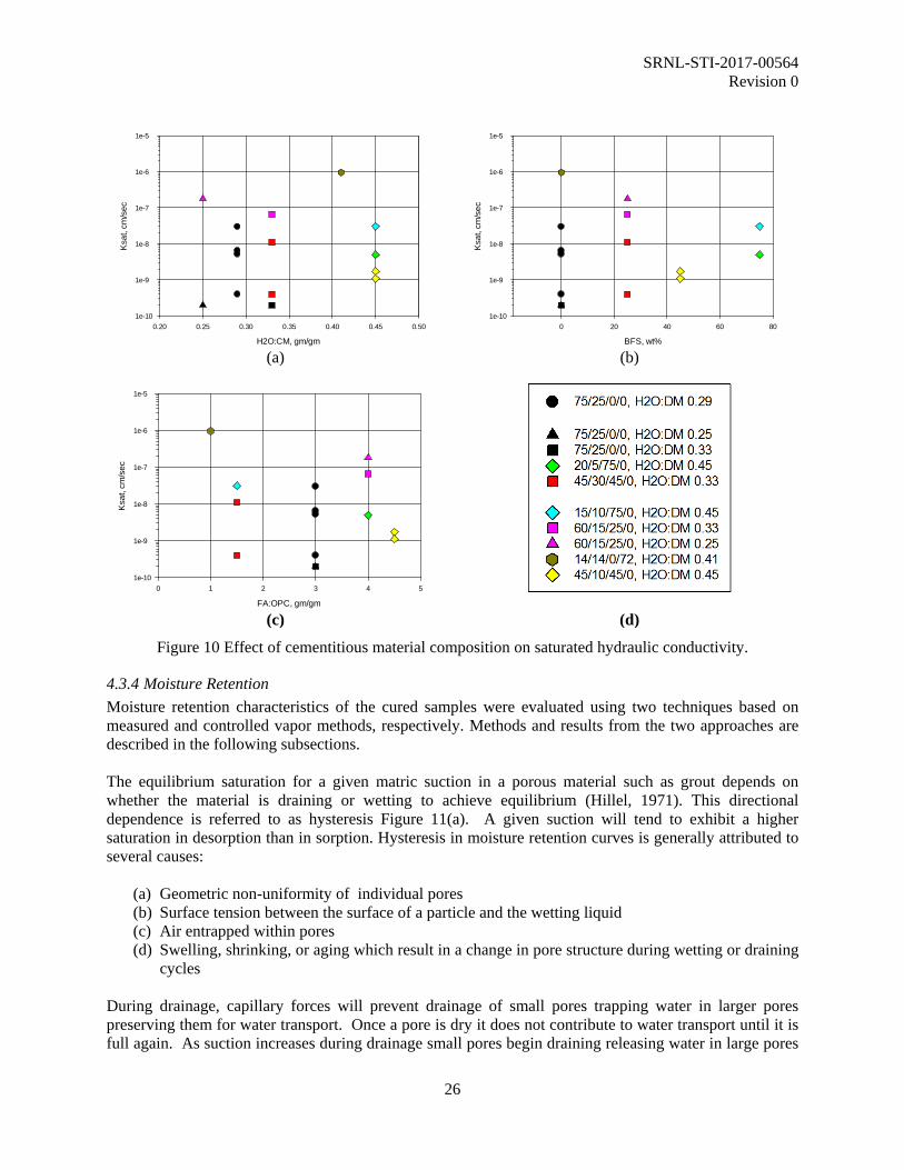
SRNL-STI-2017-00564 Revision 0
26
H2O:CM, gm/gm
0.20 0.25 0.30 0.35 0.40 0.45 0.50
Ksa
t, cm
/sec
1e-10
1e-9
1e-8
1e-7
1e-6
1e-5
BFS, wt%
0 20 40 60 80
Ksa
t, cm
/sec
1e-10
1e-9
1e-8
1e-7
1e-6
1e-5
(a) (b)
FA:OPC, gm/gm
0 1 2 3 4 5
Ksa
t, cm
/sec
1e-10
1e-9
1e-8
1e-7
1e-6
1e-5
(c) (d)
Figure 10 Effect of cementitious material composition on saturated hydraulic conductivity.
4.3.4 Moisture Retention Moisture retention characteristics of the cured samples were evaluated using two techniques based on measured and controlled vapor methods, respectively. Methods and results from the two approaches are described in the following subsections. The equilibrium saturation for a given matric suction in a porous material such as grout depends on whether the material is draining or wetting to achieve equilibrium (Hillel, 1971). This directional dependence is referred to as hysteresis Figure 11(a). A given suction will tend to exhibit a higher saturation in desorption than in sorption. Hysteresis in moisture retention curves is generally attributed to several causes:
(a) Geometric non-uniformity of individual pores (b) Surface tension between the surface of a particle and the wetting liquid (c) Air entrapped within pores (d) Swelling, shrinking, or aging which result in a change in pore structure during wetting or draining
cycles During drainage, capillary forces will prevent drainage of small pores trapping water in larger pores preserving them for water transport. Once a pore is dry it does not contribute to water transport until it is full again. As suction increases during drainage small pores begin draining releasing water in large pores

SRNL-STI-2017-00564 Revision 0
27
this causes hydraulic conductivity to decrease at lower saturation. During wetting, large pores remain empty until the capillary pressure is high enough in small pores to overcome surface tension and contact angle effects of the adjacent large pore and let liquid re-wet the large pore. This is often referred to as the ink bottle effect Figure 12. Since large pores wet last hydraulic conductivity is lower during wetting relative to draining for the same suction or saturation Figure 11(b). Stephens (1996) identified a similar hysteresis effect on hydraulic conductivity where Krel in a draining condition will be greater than Krel during wetting for the same suction, Figure 11(b).
(a) Source :(Hillel, 1971)
(b) Source : (Stephens, 1996)
Figure 11 Hysteresis of water content and hydraulic conductivity.
Source (Hillel, 1971)
Figure 12 Illustration of ink bottle effect (a) draining; (b) wetting.
Draining
Draining
Wetting
Wetting

SRNL-STI-2017-00564 Revision 0
28
4.3.4.1 Measured Vapor Pressure A measured vapor pressure method (chilled mirror) (ASTM, D 6836– 08) was used to evaluate the moisture retention characteristics of the SSW grout formulations. The chilled mirror hygrometer (Decagon Devices WP4C) uses the chilled mirror dew point technique to measure the moisture potential of porous materials ((Nimmo and Winfield, 2002); (Gee et al., 1992)). Total moisture potential is the sum of osmotic and matric potential (neglecting hydrostatic pressure and gravitational effects). Samples from each of the SSW grout formulations were prepared for testing in the WP4C hygrometer by crushing the grout using a mortar and pestle. The crushed grout was then sieved to produce bulk powder with a particle size of 2 mm or less. The bulk powder from each formulation was oven dried and subsequently rewetted with deionized water for testing in the WP4C hygrometer. For a typical test, samples are wetted to near saturation, measured in the WP4C hygrometer, and subsequently dried to achieve a lower moisture potential before testing again. Samples are allowed to equilibrate for at least 24 hours between measurements. This process simulates a desorption cycle for porous materials. A new approach was developed for the SSW grout formulations to simulate the sorption cycle for a porous material and derive van Genuchten parameters for the sorption moisture retention curve. For each SSW grout formulation, two grams of oven dried material were weighed into each of several sample cups. The samples were incrementally rewetted with water to create a distribution of moisture contents based on the measured porosity of each formulation. Samples were allowed to equilibrate for at least 24 hours prior to testing. Appendix B contains the data for the samples tested using the chilled mirror method. Figure 13 shows desorption and sorption curves for Mix 1 developed using data from the chilled mirror and Controlled Vapor Pressure (CVP) methods and Table 9 contains the corresponding van Genuchten parameters for each moisture retention curve derived using the chilled mirror methods.

SRNL-STI-2017-00564 Revision 0
29
Figure 13 van Genuchten curves showing the effect of hystersis on saturation.
4.3.4.2 Controlled Vapor Pressure A CVP method was used to determine van Genuchten parameters for desorption moisture retention curves for each of the SSW grout formulations. For the CVP method, vacuum saturated, intact wafers approximately ½ inch thick were placed above a saturated salt solution inside a sealed container as shown in Figure 14. The saturated salt solution produces a constant relative humidity (RH) in the headspace of the sealed container. Relative humidity is then related to total water potential using the Kelvin equation (Nimmo and Winfield, 2002). Each puck drains by evaporation until pore water in the sample is at equilibrium with the vapor pressure in the headspace of the container. At equilibrium, the material is assumed to attain the same total potential as the vapor in the headspace of the container (Nimmo and Winfield, 2002). This CVP method produces data for determining the parameters for a desorption van Genuchten curve. Each wafer was weighed prior to placing it in the sealed container with the salt solution. Periodically, the samples were removed and weighed to determine whether equilibrium had been reached. When the mass change between successive readings was generally less than 0.5%, testing was deemed complete. At the conclusion of the CVP testing, wafers from each formulation were used to determine, equilibrium saturation, dry bulk density and porosity. These results are presented in Table 8. Figure 13 shows a comparison of the desorption curve derived from the chilled mirror method to the desorption curve derived from the CVP equilibrium method. Appendix C contains the data for the samples tested using the CVP method.

SRNL-STI-2017-00564 Revision 0
30
Figure 14 Grout wafers used in the CVP method equilibarting in a sealed dessicator containing a saturated salt solution.
4.3.5 Interpretation of Results The results from the measured vapor equilibrium (chilled mirror) tests and the controlled vapor equilibrium tests were analyzed to determine the van Genuchten curve fitting parameters (Van Genuchten, 1980). Non-linear regression analysis in Microsoft Excel was used to fit the measured moisture retention data for the grout samples, see Figure 15. The closed form analytical expression developed by van Genuchten which predicts soil moisture content as a function of pressure was used for this analysis. The relationship is given as:
[ ]mn
rsr
hh
)(1)(
α
θθθθ
+
−+=
0≤h (3)
sh θθ =)( 0>h (4) Where:
θ(h) is moisture content at the pressure head h,, θr is residual moisture content, θs is the saturated moisture content, h is pressure head, α is a constant related to the inverse of the air-entry pressure, and n is a measure of the pore-size distribution.

SRNL-STI-2017-00564 Revision 0
31
The constraint m = 1 – 1/n was used as suggested by van Genuchten ((Van Genuchten, 1980); (Van Genuchten et al., 1991)). The predicted moisture retention curves were based on moisture retention data only; no unsaturated hydraulic conductivity data were available for the samples. RETC’s (USDA, 1998) van Genuchten m = 1 – 1/n retention curve model was used to estimate curve fitting parameters (θr, θs, α, n). The curve fitting parameters (θr, θs, α, n) (from RETC (USDA, 1998)) were used to calculate the effective saturation (or reduced water content), Se, at incremental pressure heads according to:
[ ]mnr
re
hSSSS
)(1
11 α+
=−−
=
(5)
Where Sr denotes residual saturation. Using Se, the relative hydraulic conductivity (Krel) was calculated at incremental pressure heads using the Mualem-van Genuchten type function
( )[ ]2/111 mme
Lerel SSK −−= (6)
where L is an empirical pore-connectivity parameter and assumed to be 0.5. Saturation (S) was calculated at various pressure heads according to
( )[ ]
+
−+= mn
rr
h
SSSα1
1
(7)
where residual saturation, Sr, is equal to θr/θs (the residual moisture content divided by the saturated moisture content). The resulting van Genuchten transport parameters are provided in Table 9 and Table 10. Figure 16 shows sorption moisture retention curves for the SSW grout formulations that were derived using data from chilled mirror sorption method. Desorption moisture retention curves developed using data from the CVP method are shown in Figure 18. Figure 16 and Figure 18 cover the range of matric suction used in each test. Appendix D and Appendix E contain the characteristic curves for each ot the samples tested using the chilled mirror and controlled vapor equilibrium method.

SRNL-STI-2017-00564 Revision 0
32
Table 8 Physical Properties of Hanford Secondary Waste Formulations determined on wafer samples used for CVP testing.
Batch ID
Dry Bulk Density (g/cm3)
Porosity (cm3/cm3)
Mix 1 1.626 0.354 Mix 1a 1.638 0.357 Mix 2 1.729 0.322 Mix 3 1.541 0.389
Mix 5* 1.331 0.533 Mix 6 1.606 0.365 Mix 6a 1.601 0.377 Mix 9* 1.333 0.494 Mix 10 1.548 0.397 Mix 11 1.696 0.327 Mix 121 1.89 0.30 Mix 13 1.330 0.480 Mix 13a 1.329 0.491 PFX004 1.624 0.368 PFX006 1.622 0.373
1 Measured on Ksat sample

SRNL-STI-2017-00564 Revision 0
33
Table 9 Van Genuchten transport parameters using chilled mirror equilibrium model for mixes in Phase 1.
Mix1,2 θs
(cm3/cm3) θr
(cm3/cm3) α
(1/cm) n m r2
Curve Type
PA Data Pkg, paste 0.603 0.000 6.47E-06 3.104 0.587 -
Desorption
PFX-003 0.352 0.000 3.51E-06 1.822 0.451 0.98 Desorption PFX-005 0.371 0.000 2.72E-06 1.847 0.459 0.94 Desorption PFX3 0.361 0.000 1.76E-05 1.472 0.320 0.98 Adsorption 1 0.348 0.000 2.73E-06 1.874 0.466 0.99 Desorption 14 0.348 0.000 1.96E-05 1.498 0.333 0.97 Adsorption 1a5 0.348 0.000 1.84E-05 1.616 0.381 0.99 Adsorption 2 0.322 0.000 5.89E-06 1.892 0.471 0.97 Adsorption 3 0.385 0.000 1.18E-05 1.737 0.424 0.96 Adsorption 5 0.515 0.000 2.13E-05 1.689 0.408 0.96 Adsorption 6 0.372 0.000 2.86E-06 2.600 0.615 0.91 Adsorption 6a5 0.372 0.000 1.51E-05 1.540 0.350 0.98 Adsorption 8 0.510 0.000 1.25E-05 2.091 0.522 0.98 Adsorption 10 0.414 0.000 1.67E-05 1.774 0.436 0.94 Adsorption 104 0.414 0.000 2.04E-05 1.721 0.419 0.99 Adsorption 11 0.330 0.000 3.68E-06 2.547 0.607 0.97 Adsorption 12 0.302 0.000 1.91E-04 1.346 0.592 0.95 Adsorption 13 0.480 0.000 5.23E-06 2.452 0.592 0.95 Adsorption 134 0.480 0.000 9.49E-06 2.167 0.538 0.96 Adsorption Mix 13a5 0.480 0.000 1.20E-05 2.161 0.537 0.97 Adsorption
1Data analyzed using Mualem relationship between n and m where m = 1 – 1/n. 2θs fixed to average measured porosity for each solid secondary waste formulation. 3PFX-003 and PFX-005 combined. 4Re-run 5Replicate mix
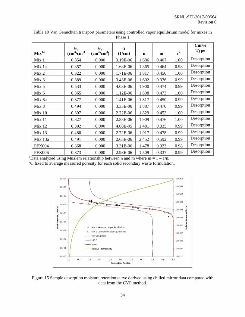
SRNL-STI-2017-00564 Revision 0
34
Table 10 Van Genuchten transport parameters using controlled vapor equilibrium model for mixes in Phase 1
Mix1,2 θs
(cm3/cm-3 θr
(cm3/cm3) α
(1/cm) n m r2
Curve Type
Mix 1 0.354 0.000 3.19E-06 1.686 0.407 1.00 Desorption
Mix 1a 0.357 0.000 1.68E-06 1.865 0.464 0.98 Desorption
Mix 2 0.322 0.000 1.71E-06 1.817 0.450 1.00 Desorption
Mix 3 0.389 0.000 3.43E-06 1.602 0.376 0.99 Desorption
Mix 5 0.533 0.000 4.03E-06 1.900 0.474 0.99 Desorption
Mix 6 0.365 0.000 1.12E-06 1.898 0.473 1.00 Desorption
Mix 6a 0.377 0.000 1.41E-06 1.817 0.450 0.99 Desorption
Mix 8 0.494 0.000 3.33E-06 1.887 0.470 0.99 Desorption
Mix 10 0.397 0.000 2.22E-06 1.829 0.453 1.00 Desorption
Mix 11 0.327 0.000 2.83E-06 1.909 0.476 1.00 Desorption
Mix 12 0.302 0.000 4.08E-05 1.481 0.325 0.99 Desorption
Mix 13 0.480 0.000 2.72E-06 1.917 0.478 0.99 Desorption
Mix 13a 0.491 0.000 2.63E-06 2.452 0.592 0.99 Desorption
PFX004 0.368 0.000 3.31E-06 1.478 0.323 0.98 Desorption
PFX006 0.373 0.000 2.98E-06 1.509 0.337 0.99 Desorption 1Data analyzed using Mualem relationship between n and m where m = 1 – 1/n. 2θs fixed to average measured porosity for each solid secondary waste formulation.
Figure 15 Sample desorption moisture retention curve derived using chilled mirror data compared with data from the CVP method.

SRNL-STI-2017-00564 Revision 0
35
In the data package for the IDF PA, (Flach et al., 2016), the expected exposure condition for buried IDF waste is considered to be on the order of 1000 cm H2O suction. Figure 17 and Figure 19 show the relative permeability function for each SSW grout formulation as determined using chilled mirror and CVP method for the relative permeability only ranging from 0.1 to 1.0 to allow better inspection of the range of interest in the IDF PA data package i.e suction ≤ 1000 cm H2O. Relative permeability for any of the mixes tested is less than or equal to the relative permeability of the baseline material in the IDF PA data package. Because the SSW waste forms are likely to be nearly saturated after curing the initial matric suction in the SSW grout is expected to be near zero. When this waste form is buried in Hanford sediments with an expected matric potential of -1000 cm H2O the waste form will be in a draining condition and the desorption moisture retention curve should be used to simulate conditions within the waste form. Because the waste form will be draining the hydraulic conductivity will be decreasing as it equilibrates with the soil it is buried in.
(a)
(b)
(c)
(d)
Figure 16 Comparison of sorption relative permeability curves for SSW grout formulations using van Genuchten parameters derived from the chilled mirror method.

SRNL-STI-2017-00564 Revision 0
36
(a)
(b)
(c)
(d)
Figure 17 Comparison of sorption relative permeability curves for SSW grout formulations for the region of interest using van Genuchten parameters derived from the chilled mirror method.
Results from duplicate tests generally are in agreement especially for the range of interest. The relative permeability curves from replicate samples for Mix 1 and 6 show more relative difference than do relative permeability curves for Mix 13. This may possibly be due to the effect of fibers in Mixes 1 and 6 as previously described for Mix 6. Mix 13 does not contain fibers and there is less difference between the replicate samples. Krel for Mix 12 decreases more rapidly at lower suctions than the other mixes as shown in graph (a) of Figure 17 and Figure 19. Mix 12 contains sand, 72% w/w, and none of the other mixes do. The presence of sand in grouts decreases the entry pressure and as a result drainage ensues at lower pressures reducing Krel. Air entry pressure is inversely proportional to the van Genuchten parameter α. α for Mix 12 is larger than the other mixes which decreases air entry pressure and there drainage begins at lower suction. Drainage reduces permeability by reducing the number of remaining saturated pores transporting fluid. Furthermore the largest pores drain first so transport must occur in the remaining saturated pores which are smaller. This result is consistent with the findings in Flach 2016 in which mixes with aggregate had larger values for α than the mixes without aggregate.

SRNL-STI-2017-00564 Revision 0
37
(a)
(b)
(c)
(d)
Figure 18 Comparison of desorption relative permeability curves for SS grout formulations formulations using van Genuchten parameters derived from the CVP method.

SRNL-STI-2017-00564 Revision 0
38
(a)
(b)
(c)
(d)
Figure 19 Comparison of desorption permeability curves for SSW grout formulations over the region of interest using van Genuchten parameters derived from the CVP method.

SRNL-STI-2017-00564 Revision 0
39
5.0 Phase 2 Results Samples of simulated waste forms were prepared in Phase 2. The waste forms consisted of drained sRF resin that have been previously used in tests to determine mechanical properties and grout mixes selected from Phase1. Three different grouts and two different sRF loadings are being tested (see Table 11). Mix 1 is the baseline mix in the IDF PA. Mix 5 has the highest BFS content and preliminary data from Phase 1 indicate it has low hydraulic conductivity when compared to other mixes with 0.75 w/w content BFS. Mix 13 was selected to include a grout with mid-range BFS content (0.45 w/w) in the CM and has well established properties from similar studies of Mix 13 prepared with 5M Na salt solution. Preliminary results from Phase 1 show that all three mixes have similar water retention curves similar to other mixes in Phase 1.
Table 11 Mixes and waste loading to be studied in Phase 2
Mix H2O:CM
(w/w) FA/OPC/BFS
(w/w)
Waste Loading
(v/v) Comment 1.1 0.29 75/25/0 0.10 current Mix 5 used in burial ground 1.3 0.29 75/25/0 0.30
5.1 0.45 20/5/75 0.10 5.3 0.45 20/5/75 0.30
13.1 0.45 45/10/45 0.10 13.3 0.45 45/10/45 0.30 𝑁𝑁𝑁𝑁𝑁𝑁𝑁𝑁: 𝑣𝑣 𝑣𝑣⁄ =
𝑣𝑣𝑠𝑠𝑠𝑠𝑠𝑠𝑣𝑣𝑇𝑇𝑇𝑇𝑇𝑇𝑇𝑇𝑇𝑇
Grout batches for the simulated waste forms were prepared for the mixes in Table 11 using ASTM C-150 Type I-II Cement (OPC), BFS, Class F fly ash (FA), sand, admix BASF Pozzolith 80 and BASF Master Fiber M100 from samples provided by American Rock Products, Lafarge Northwest, and BASF. The elemental composition of the cementitious materials used in this study was determined using x-ray fluorescence, results are presented in Table 2. Waste forms were prepared by mixing drained sRF with a predetermined amount of water based on H2O:CM for the specific mix in a beaker using an overhead mixer. Once the drained sRF resin and water were blended and mixed for two minutes of mixing, the DM consisting of CM was added to the beaker containing water and drained sRF resin as it was being stirred by an overhead mixer. Mixer speed was adjusted to maintain a vortex in the grout as DM was added. Once all of the DM was included, the admix and fiber were added. Fiber was shredded by hand using tweezers to breakup the fiber into smaller assemblages prior to adding to the grout. After all ingredients were in the grout, the grout was stirred until an overall mixing period of 15 minutes had been completed ensuring there was a vortex at all times. This mixing method was developed to mimic an in container solidification process that may be used to solidify sRF resin (see Figure 20). Occasionally the mixer was stopped to “burp” the grout to remove air pockets that affect mixing. Once the mixing was complete the grout was immediately decanted for fresh property testing and into molds.

SRNL-STI-2017-00564 Revision 0
40
Figure 20 Conceptual model for solidifying drained sRF resin.
The sRF resin was drained prior to mixing using a disposable filter unit that had a 500 mL upper chamber and 0.45µm nylon filter. A predetermined volume of sRF resin was decanted into the upper filter chamber and allowed to gravity drain for 3-4 hours. Following drainage a small sample of drained sRF resin was removed for drying at 105°C to determine gravimetric water content and the remainder was used to prepare the simulated waste form. Results from sRF water content determination are provided in Table 12. A scoping waste form was prepared prior to the waste forms used for testing to assess the method for preparing the waste forms. A waste loading of 0.2 v/v was used with Mix 1 to prepare the simulated waste form and evaluate how well the sRF resin would stay mixed in the grout while it cured. Figure 21 (a) shows a photograph of a split sample originally used to assess curing and (b) is a slice from a 3d-µCT scan of a 5cm diameter x 10cm long monolith from the same test batch. Both images show the sRF is homogeneously distributed in the grout. Gray specks in the µCT image are the resin and black swirls in the right center is air entrained in a clump of fiber.

SRNL-STI-2017-00564 Revision 0
41
(a) (b)
Figure 21 Photograph (a) and µCT slice (b) of simulated waste form with 0.2 v/v sRF resin loading Mix 1 grout.
Samples of the simulated waste form were removed from capped molds which cured for 28 days at room temperature in a sealed bag containing a moist handi-wipe. Some of the samples were sent off to be prepared for water retention and saturated hydraulic conductivity testing. Another one of the molds was used to determine initial saturation. Samples used for initial saturation were measured and weighed immediately after being removed from the molds. After measuring and drying, the samples were placed in an oven at 105°C for drying to determine dry weight of the waste form cylinder. Following drying, the samples were re-saturated with water under a vacuum to determine saturated weight. Sample, initial, dry, and saturated weight along with sample dimensions were used to estimate initial saturation, dry bulk density and porosity as given in Table 12. Additional results for mixes with 0.3 v/v sRF resin loading and results from water retention and Ksat testing for all Phase 2 samples will be provided in a subsequent report.

SRNL-STI-2017-00564 Revision 0
42
Table 12 Initial results from simulated waste forms with 0.1 v/v sRF resin loading.
Mix sRF (v/v)
Drained sRF Water Content, gm/gm
Initial Saturation
Dry Bulk Density, gm/cm3
Porosity Solids
Density, gm/cm3
Mix 1.1 0.1 0.66 0.92 1.45 0.42 2.50 Mix 5.1 0.1 0.69 0.97 1.15 0.58 2.75 Mix 13.1 0.1 0.68 0.96 1.16 0.54 2.54
Note: Particle density of sRF resin = 0.45 gm/cm3

SRNL-STI-2017-00564 Revision 0
43
6.0 Summary and Conclusions Ten of the 13 grout mixes selected for testing in this scoping study were successfully prepared and tested for fresh and cured properties. Two of the mixes required increased H2O:CM ratios and one mix was abandoned due to low flow at 0.25 H2O:CM. Fresh properties were within the range expected for these mixes. All mixes in this study have had fresh properties that would generally make them suitable for use in solidification and encapsulation of SSW. Additional testing is planned to confirm the results of this initial testing and to assess the potential variability of the baseline grout mix, Hanford Grout Mix 5, which is being used for current disposal activities at the Hanford Site. All mixes achieved sufficient compressive strength for consideration in the use of solidification or encapsulation of SSW followed by subsequent land disposal assuming typical compressive strength requirements for similar applications. The range of saturated hydraulic conductivities determined for mixes in this study is consistent with the overall ranges suggested in the Data Package of the IDF PA (Flach et al., 2016). The mean of the saturated hydraulic conductivities for the four samples of the baseline grout mix (two prepared by PermaFix and 2 prepared by SRNL) was within two standard deviations of the mean as reported in the IDF data package. The baseline recipe contains fiber which requires aggregate to ensure good incorporation into the mix. However, the baseline recipe does not contain aggregate and as a result clumping was experienced in preparation of batches in the laboratory. Examination of a 3d-μCT scan revealed the presence of a clump of fibers in the baseline sample with increased saturated hydraulic conductivity. The presence of a clump of fibers in a mold sample could possibly result in a higher saturated hydraulic conductivity depending on its’ relation to the size of the mold. This possibility was confirmed through conversations with the batch plant. If this is determined to be a critical issue testing of samples prepared without fiber in future studies may be warranted. The benefits of including fiber may also need to be reconsidered in the context of the potential for increased permeability Desorption and sorption moisture retention characteristics for all of the mixes were similar to those for the baseline mix used in the IDF PA data package. In all cases the mixes tested had lower relative hydraulic conductivities than that of the baseline mix for the same matric suction in the region of interest. The grouts tested exhibited hysteresis in moisture retention resulting in higher saturation for a given equilibrium matric suction during drainage when compared to the saturation during wetting for the same equilibrium matric suction. Likewise, a higher relative hydraulic conductivity would be expected during drainage than during wetting for the same equilibrium matric suction. Because the SSW waste forms are likely to be nearly saturated after curing the initial matric suction in the SSW grout is expected to be near zero. When this waste form is buried in Hanford sediments with an expected matric potential of -1000 cm H2O the waste form will be in a draining condition and the desorption moisture retention curve should be used to simulate conditions within the waste form. Because the waste form will be draining the hydraulic conductivity will be decreasing as it equilibrates with the soil it is buried in. As of this report four simulated waste forms have been prepared for Phase 2 testing. The waste forms were prepared by incorporation of sRF resin into the mixes selected from Phase 1 at a loading of 0.1 v/v. Additional waste forms will be prepared and tested using the same mixes and a waste loading of 0.3 v/v. Prior to preparing the waste forms for testing a scoping waste form was prepared to assess the methods selected for preparing them. This sample has a 0.2 v/v waste loading. Imaging of the scoping sample indicated the sRF resin was well mixed into the grout and remained homogenously distributed throughout during curing.

SRNL-STI-2017-00564 Revision 0
44
7.0 References ASTM (C39/C39M – 15a). Standard Test Method for Compressive Strength of Cylindrical Concrete
Specimens. West Conshohocken, PA. ASTM (C 191-13). Standard Test Method for Time of Setting of Hydraulic Cement by Vicat Needle.
West Conshohocken, PA. ASTM (C 1679). Standard Practice for Measuring Hydration Kinetics of Hydraulic Cementitious
Mixtures Using Isothermal Calorimetry. West Conshohocken, PA. ASTM (D5084-10). Standard Test Methods for Measurement of Hydraulic Conductivity of Saturated
Porous Materials Using a Flexible Wall Permeameter. West Conshohocken, PA. ASTM (D 1475-13). Standard Test Method for Density of Liquid Coatings, Inks, and Related Products.
West Conshohocken, PA. ASTM (D 6836– 08). Standard Test Methods for Determination of the Soil Water Characteristic Curve
for Desorption Using Hanging Column, Pressure Extractor, Chilled Mirror Hygrometer, or Centrifuge. West Conshohocken, PA.
Cozzi, A. D., Dixon, K. L., Hill, K. A., and Nichols, R. L. (2017). "Liquid Secondary Waste: Waste Form Formulation and Qualification," Rep. No. SRNL-STI-2-17-00116, Rev. B. Savannah River National Laboratory, Savannah River Site, Aiken, SC.
Flach, G. P., Kaplan, D. I., Nichols, R. L., Seitz, R. R., and Serne, R. J. (2016). "Solid Secondary Waste Data Package Supporting Hanford Integrated Disposal Facility Performance Assessment " Rep. No. SRNL-STI-2016-00175. Savannah River National Laboratory, Aiken, SC.
Gee, G. W., Campbell, M. D., Campbell, G. S., and Campbell, J. H. (1992). Rapid Measurement of Low Soil Water Potentials using a Water Activity Mete. Soil Science Society of America Journal 56, 1068-1070.
Hillel, D. (1971). "Soil and Water: Physical Principles and Processes," Academic Press, Inc., New York, NY.
Kay, R., Surman, J., and Shete, D. (2017). "DFLAW Solid Secondary Wastes - Phase 2 Review of UK ILW and LLW Immobilization," Rep. No. DBD/4909//PRJ/RP/004 Rev. C. DbD Limited, Cheshire, UK.
Nichols, R. L., and Kaplan, D. I. (2017). "Task Technical and Quality assurance Plan for Hanford Solid Secondary Waste Formulation Development and Waste Form Qualification," Rep. No. SRNL-RP-2016-00735, Rev. 2. Savannah River National Laboratory, Aiken, SC.
Nimmo, J. R., and Winfield, K. A., eds. (2002). "Water Retention and Storage: Miscellaneous Methods." Soil Science Society of America.
Scrivener, K. L., and Nemati, K. M. (1995). The Percolation of Pore Space in the Cement Paste/Aggregate Interfacial Zone of Concrete. Cement & Concrete Research 26, 35-40.
Seitz, R. R. (2017). "Examples of Disposal Alternatives for Solid Secondary Waste," Rep. No. SRNL-STI-2017-00508. Savannah River National Laboratory, Aiken, SC.
Smith, K. W. (2015). Updated Evaluation of Waste Treatment and Immobilization Plant Secondary Dangerous Waste Treatment and Disposal for 2015 Dangerous Waste Permit Submittal. (J. A. Hedges, ed.), Richland, WA.
Stephens, D. B. (1996). "Vadose zone hydrology," Lewis Publishers, Boca Raton, FLA. USDA (1998). RETC for Windows, 1998. U.S. Salinity Laboratory, U.S. Department of Agriculture
(USDA). USEPA (2013). "Statistical Software for Environmental Applications for Data Sets with and without
Nondetect Observations," Rep. No. EPA/600/R-07/041. USEPA-Office of Research and Development, Washington, DC.
Van Genuchten, M. T. (1980). A Closed-form Equation for Predicting the Hydraulic Conductivity of Unsaturated Soils. Soil Science Society of America Journal 44, 892-898.

SRNL-STI-2017-00564 Revision 0
45
Van Genuchten, M. T., Leij, F. J., and Yates, S. R. (1991). The RETC Code for Qualifying the Hydraulic Functions of Unsaturated Soils. In "EPA Report 600/2-91/065". U.S. Salinity Laboratory, Riverside, CA.
WRPS (2016). "Test Specification for the Low-Activity Waste Pretreatment System Full-Scale Ion Exchange Column Test and Engineering-Scale Integrated Test (Project T5L01)," Rep. No. RPP-RPT-58683, Rev. 2, Richland, WA.

SRNL-STI-2017-00564 Revision 0
A-1
. Shear curves Appendix A

SRNL-STI-2017-00564 Revision 0
A-2
Figure 22 Mix 1 Flow Curve.
Figure 23 Mix 1a Flow Curve.
0
20
40
60
80
100
120
0 25 50 75 100 125 150 175 200 225 250 275 300 325
Shea
r Stre
ss (P
a)
Shear Rate (1/sec)
SSW - Mix 1, 12-6-2016Up Curve Hold Down Curve
0
20
40
60
80
100
120
0 25 50 75 100 125 150 175 200 225 250 275 300 325
Shea
r Stre
ss (P
a)
Shear Rate (1/sec)
SSW - Mix 1a, 12-19-2016Up Curve Hold Down Curve

SRNL-STI-2017-00564 Revision 0
A-3
Figure 24 Mix 2 Flow Curve.
Figure 25 Mix 3 Flow Curve.
0
20
40
60
80
100
120
140
160
0 25 50 75 100 125 150 175 200 225 250 275 300 325
Shea
r Stre
ss (P
a)
Shear Rate (1/sec)
SSW - Mix 2, 12-7-2016Up Curve Hold Down Curve
0
10
20
30
40
50
60
70
80
0 25 50 75 100 125 150 175 200 225 250 275 300 325
Shea
r Stre
ss (P
a)
Shear Rate (1/sec)
SSW - Mix 3, 12-7-2016Up Curve Hold Down Curve

SRNL-STI-2017-00564 Revision 0
A-4
Figure 26 Mix 4 Flow Curve.
Figure 27 Mix 6 Flow Curve.
0
10
20
30
40
50
60
70
80
90
100
110
0 25 50 75 100 125 150 175 200 225 250 275 300 325
Shea
r Stre
ss (P
a)
Shear Rate (1/sec)
SSW - Mix 4*, 12-8-2016Up Curve Hold Down Curve
0
20
40
60
80
100
120
140
0 25 50 75 100 125 150 175 200 225 250 275 300 325
Shea
r Stre
ss (P
a)
Shear Rate (1/sec)
SSW - Mix 6, 12-12-2016Up Curve Hold Down Curve

SRNL-STI-2017-00564 Revision 0
A-5
Figure 28 Mix 6a Flow Curve.
Figure 29 Mix 8 Flow Curve.
0
20
40
60
80
100
120
140
160
180
0 25 50 75 100 125 150 175 200 225 250 275 300 325
Shea
r Stre
ss (P
a)
Shear Rate (1/sec)
SSW - Mix 6a, 1-5-2017Up Curve Hold Down Curve
0
20
40
60
80
100
120
0 25 50 75 100 125 150 175 200 225 250 275 300 325
Shea
r Stre
ss (P
a)
Shear Rate (1/sec)
SSW - Mix 8, 12-13-2016Up Curve Hold Down Curve

SRNL-STI-2017-00564 Revision 0
A-6
Figure 30 Mix 10 Flow Curve.
Figure 31 Mix 11 Flow Curve.
0
10
20
30
40
50
60
70
80
0 25 50 75 100 125 150 175 200 225 250 275 300 325
Shea
r Stre
ss (P
a)
Shear Rate (1/sec)
SSW - Mix 10, 12-15-2016Up Curve Hold Down Curve
0
50
100
150
200
250
0 25 50 75 100 125 150 175 200 225 250 275 300 325
Shea
r Stre
ss (P
a)
Shear Rate (1/sec)
SSW - Mix 11, 12-15-2016Up Curve Hold Down Curve

SRNL-STI-2017-00564 Revision 0
A-7
Figure 32 Mix 13 Flow Curve.
Figure 33 Mix 13a Flow Curve.
0.0
5.0
10.0
15.0
20.0
25.0
30.0
35.0
40.0
0 25 50 75 100 125 150 175 200 225 250 275 300 325
Shea
r Stre
ss (P
a)
Shear Rate (1/sec)
SSW - Mix 13, 12-15-2016Up Curve Hold Down Curve
0.0
5.0
10.0
15.0
20.0
25.0
30.0
35.0
40.0
45.0
50.0
55.0
0 25 50 75 100 125 150 175 200 225 250 275 300 325
Shea
r Stre
ss (P
a)
Shear Rate (1/sec)
SSW - Mix 13a, 1-3-2017Up Curve Hold Down Curve

SRNL-STI-2017-00564 Revision 0
B-1
. Chilled mirror equilibrium Data for mixes in Phase 1 Appendix B

SRNL-STI-2017-00564 Revision 0
B-2
Table 13 Chilled mirror equilibrium Data for mixes in Phase1
Sample_ID Saturation
(%)
Total Potential (cm H2O)
PFX-003 1.102 16928 0.924 113701 0.858 160304 0.831 157041 0.699 290117 0.642 354361 0.573 480605 0.520 609195 0.493 646008 0.438 799989 0.397 973856 0.368 1035754 0.323 1180966 0.303 1273253 0.245 1367375 0.233 1420198 0.227 1446405 0.198 1591821 0.195 1660756 0.192 1799951 0.170 2234158 0.170 2393340 0.161 2382429
PFX-005 1.041 13970 0.947 138685 0.834 130731 0.790 152350 0.739 326114 0.640 308371 0.617 307861 0.586 644070 0.506 695058 0.465 1030452 0.416 689857 0.388 1120903

SRNL-STI-2017-00564 Revision 0
B-3
Sample_ID Saturation
(%)
Total Potential (cm H2O)
0.381 1268562 0.312 1447119 0.306 1332806 0.298 1161897 0.276 1971574 0.267 2261895 0.249 1509222 0.217 1354934 0.217 2198161 0.210 2428317 0.155 1741621 0.135 2364073 0.132 2548137 Mix PFX 1.205 7546 1.098 9790 0.953 18457 0.810 50885 0.666 97080 0.547 179781 0.384 462352 0.276 873921 Mix 1 1.038 68119 0.975 86270 0.956 104728 0.838 265337 0.801 280226 0.776 300315 0.678 459701 0.619 486724 0.614 505079 0.465 881977 0.456 861072 0.367 887687 0.333 1227058 0.329 1303743 0.274 1360849 0.270 1559801

SRNL-STI-2017-00564 Revision 0
B-4
Sample_ID Saturation
(%)
Total Potential (cm H2O)
0.248 1315980 0.224 2412715 0.220 2000228 0.220 2541305 0.220 2628799 0.200 2565881 0.194 2758306 0.193 1556538 0.154 2322060 0.142 2615950 0.141 2794711 Mix 1R 1.124 9892 0.957 11829 0.813 39770 0.677 81376 0.524 169787 0.359 433901 0.254 765930 Mix 1a 0.943 20803 0.837 46194 0.675 76277 0.548 108093 0.404 228831 0.266 514155 Mix 2 1.096 33957 0.921 68221 0.860 99119 0.735 135218 0.537 282877 0.413 377815 0.301 758282 0.170 1166384

SRNL-STI-2017-00564 Revision 0
B-5
Sample_ID Saturation
(%)
Total Potential (cm H2O)
Mix 3 0.780 102994 0.689 99833 0.634 105849 0.511 161324 0.413 257078 0.314 399332 0.248 699239 0.122 1150272 Mix 5 1.045 1122 0.917 25086 0.758 51089 0.647 62102 0.549 77705 0.518 131037 0.470 202011 0.399 120432 0.378 221285 0.344 274617 0.261 368536 0.257 250755 0.199 449605 0.154 591656 0.130 502530 0.077 1056455 Mix 6 0.877 282571 0.793 221794 0.675 274005 0.594 296338 0.469 537099 0.361 583600 0.232 1151801 0.147 1334335 Mix 6a 1.326 7138 1.246 8056 1.107 10197

SRNL-STI-2017-00564 Revision 0
B-6
Sample_ID Saturation
(%)
Total Potential (cm H2O)
0.908 34365 0.714 90247 0.583 131139 0.369 487030 0.230 967431 Mix 8 0.939 33244 0.821 70770 0.674 81580 0.537 102586 0.415 152758 0.289 265134 0.164 474997 Mix 10 1.225 4181 0.934 12135 0.744 65264 0.565 94530 0.365 205988 0.199 526698 Mix 10R 1.047 4793 0.946 8566 0.778 46806 0.618 76991 0.489 110846 0.332 213840 0.211 467247 Mix 11 1.038 91879 0.939 146639 0.800 198850 0.704 227403 0.556 308473 0.427 394029 0.275 838944 0.174 1028106

SRNL-STI-2017-00564 Revision 0
B-7
Sample_ID Saturation
(%)
Total Potential (cm H2O)
Mix 12 0.839 3161 0.636 17540 0.474 56392 0.381 129406 0.225 395559 0.084 687614 Mix 13 0.558 223630 0.504 214146 0.429 255650 0.378 337433 0.298 526392 0.229 533020 0.148 782144 0.093 1015359 Mix 13R 1.112 2345 0.986 15908 0.832 99119 0.684 104014 0.556 121248 0.421 173866 0.281 327542 0.179 533020 MIX 13a 1.104 3569 0.985 34977 0.830 59349 0.684 74543 0.555 100037 0.423 147965 0.289 279818 0.158 557596

SRNL-STI-2017-00564 Revision 0
C-1
. Controlled vapor equilibrium data for mixes in Phase 1. Appendix C

SRNL-STI-2017-00564 Revision 0
C-2
Table 14 Controlled vapor equilibrium data for mixes in Phase 1.
Pressure (cm H2O) Mix 1 Mix 1a Mix 2 Mix 6a Mix 3 Mix 5 Mix 6 Mix 8
38293 0.955 0.987 0.970 0.992 0.958 0.982 1.025 0.994 116653 0.921 0.970 0.936 0.969 0.920 0.965 0.983 0.981 396890 0.664 0.800 0.792 0.866 0.673 0.509 0.927 0.638 521158 0.637 0.755 0.748 0.822 0.629 0.452 0.862 0.505 771771 0.488 0.598 0.663 0.699 0.545 0.356 0.757 0.392
1551051 0.300 0.491 0.443 0.504 0.364 0.202 0.529 0.256 3050396 0.218 0.230 0.274 0.241 0.205 0.135 0.322 0.157
Pressure (cm H2O) Mix 10 Mix 11 Mix 12 Mix 13 Mix 13a Mix PFX-
004 Mix PFX-
006
38293 0.986 0.993 0.711 0.993 0.992 0.952 0.954 116653 0.965 0.980 0.438 0.980 0.986 0.912 0.914 396890 0.737 0.652 0.282 0.652 0.584 0.711 0.730 521158 0.677 0.577 0.577 0.492 0.730 0.730 771771 0.517 0.475 0.208 0.475 0.374 0.589 0.610
1551051 0.330 0.240 0.109 0.240 0.156 0.387 0.439 3050396 0.188 0.146 0.095 0.146 0.139 0.295 0.309

SRNL-STI-2017-00564 Revision 0
D-1
. Chilled mirror equilibrium graphs for mixes in Phase 1 Appendix D

SRNL-STI-2017-00564 Revision 0
D-2
Figure 34 Characteristic Curves for Solid Secondary Waste Mix PFX-003 – Measured Vapor Pressure
Figure 35 Characteristic Curves for Solid Secondary Waste Mix PFX-005 – Measured Vapor Pressure

SRNL-STI-2017-00564 Revision 0
D-3
Figure 36 Characteristic Curves for Solid Secondary Waste Mix PFX– Measured Vapor Pressure
Figure 37 Characteristic Curves for Solid Secondary Waste Mix 1 – Measured Vapor Pressure

SRNL-STI-2017-00564 Revision 0
D-4
Figure 38 Characteristic Curves for Solid Secondary Waste Mix 1R – Measured Vapor Pressure
Figure 39 Characteristic Curves for Solid Secondary Waste Mix 1a – Measured Vapor Pressure

SRNL-STI-2017-00564 Revision 0
D-5
Figure 40 Characteristic Curves for Solid Secondary Waste Mix 2 – Measured Vapor Pressure
Figure 41 Characteristic Curves for Solid Secondary Waste Mix 3 – Measured Vapor Pressure

SRNL-STI-2017-00564 Revision 0
D-6
Figure 42 Characteristic Curves for Solid Secondary Waste Mix 5 – Measured Vapor Pressure
Figure 43 Characteristic Curves for Solid Secondary Waste Mix 6 – Measured Vapor Pressure

SRNL-STI-2017-00564 Revision 0
D-7
Figure 44 Characteristic Curves for Solid Secondary Waste Mix 6a – Measured Vapor Pressure
Figure 45 Characteristic Curves for Solid Secondary Waste Mix 8 – Measured Vapor Pressure

SRNL-STI-2017-00564 Revision 0
D-8
Figure 46 Characteristic Curves for Solid Secondary Waste Mix 10 – Measured Vapor Pressure
Figure 47 Characteristic Curves for Solid Secondary Waste Mix 10R – Measured Vapor Pressure

SRNL-STI-2017-00564 Revision 0
D-9
Figure 48 Characteristic Curves for Solid Secondary Waste Mix 11 – Measured Vapor Pressure
Figure 49 Characteristic Curves for Solid Secondary Waste Mix 12 – Measured Vapor Pressure

SRNL-STI-2017-00564 Revision 0
D-10
Figure 50 Characteristic Curves for Solid Secondary Mix 13 – Measured Vapor Pressure
Figure 51 Characteristic Curves for Solid Secondary Mix 13 – Measured Vapor Pressure

SRNL-STI-2017-00564 Revision 0
E-1
. Controlled vapor equilibrium graphs for mixes in Phase 1. Appendix E
Figure 52 Characteristic Curves for Solid Secondary Mix 1 – Controlled Vapor Pressure
Figure 53 Characteristic Curves for Solid Secondary Mix 1a – Controlled Vapor Pressure

SRNL-STI-2017-00564 Revision 0
E-2
Figure 54 Characteristic Curves for Solid Secondary Mix 2 – Controlled Vapor Pressure
Figure 55 Characteristic Curves for Solid Secondary Mix 3 – Controlled Vapor Pressure

SRNL-STI-2017-00564 Revision 0
E-3
Figure 56 Characteristic Curves for Solid Secondary Mix 5 – Controlled Vapor Pressure
Figure 57 Characteristic Curves for Solid Secondary Mix 6 – Controlled Vapor Pressure

SRNL-STI-2017-00564 Revision 0
E-4
Figure 58 Characteristic Curves for Solid Secondary Mix 6a – Controlled Vapor Pressure
Figure 59 Characteristic Curves for Solid Secondary Mix 8 – Controlled Vapor Pressure

SRNL-STI-2017-00564 Revision 0
E-5
Figure 60 Characteristic Curves for Solid Secondary Mix 10 – Controlled Vapor Pressure
Figure 61 Characteristic Curves for Solid Secondary Mix 11 – Controlled Vapor Pressure

SRNL-STI-2017-00564 Revision 0
E-6
Figure 62 Characteristic Curves for Solid Secondary Mix 12 – Controlled Vapor Pressure
Figure 63 Characteristic Curves for Solid Secondary Mix 13 – Controlled Vapor Pressure

SRNL-STI-2017-00564 Revision 0
E-7
Figure 64 Characteristic Curves for Solid Secondary Mix 13a – Controlled Vapor Pressure
Figure 65 Characteristic Curves for Solid Secondary Mix PFX-004 – Controlled Vapor Pressure

SRNL-STI-2017-00564 Revision 0
E-8
Figure 66 Characteristic Curves for Solid Secondary Mix PFX-006 – Controlled Vapor Pressure