technical report: development of a network of...

TECHNICAL REPORT: Development of a Network of No-take Zones Building on Community Based

Management Initiatives for the Island Province of Kadavu, Fiji.

Hans Karl Wendt, James Comley. Institute of Applied

Science, University of the South Pacific, Suva, Fiji

Award: NA08NOS4630332

Table of Contents 1 Introduction ............................................................................................................ 1

1.1 Community Based Management in Fiji ............................................................. 1

1.2 Kadavu Island .................................................................................................... 2

2 Methods and Results .............................................................................................. 5 2.1 Developing the Provincial Vision- and contextualizing networking criteria..... 5

2.2 Habitat characterization and mapping................................................................ 7

2.2.1 Collection of ground - truthing field data .............................................. 7 2.2.2 Classifying field data ........................................................................... 10 2.2.3 Image data ............................................................................................ 12 2.2.4 Creating habitat maps........................................................................... 12 2.2.5 Accuracy assessment of habitat maps .................................................. 14 2.2.6 Final habitat map for Kadavu............................................................... 14

2.3 Reserve design planning .................................................................................. 19

2.4 Mapping socio-cultural variables and resource use pattern ............................. 19

2.4.1 Storing collected data........................................................................... 22 2.4.2 Validation and standardization of fishing use layers ........................... 22 2.4.3 Creating an enforceability distance layer............................................. 23 2.4.4 Creating a disputed areas layer ............................................................ 24

2.5 Assessment of the pre-existing network and gap analysis ............................... 28

2.5.1 Representation...................................................................................... 28 2.5.2 Replication ........................................................................................... 30 2.5.3 Ecological linkages .............................................................................. 33 2.5.4 Long - term protection ......................................................................... 35 2.5.5 Maximising the contribution of individual no-take zones to the overall network .............................................................................................................. 36

2.6 Reserve design planning .................................................................................. 37

2.6.1 Marine reserve software....................................................................... 37 2.6.2 Assembling primary input files............................................................ 38 2.6.3 Community targets ............................................................................... 40 2.6.4 Conservation features........................................................................... 40 2.6.5 Planning Units and costs ...................................................................... 40 2.6.6 Zones .................................................................................................... 43 2.6.7 Planning unit lock ................................................................................ 43 2.6.8 Summary input files ............................................................................. 43 2.6.9 Running Marxan .................................................................................. 44 2.6.10 Examining runs .................................................................................... 44

2.7 Supplementing the existing- communicating design results............................ 46

2.7.1 Presenting results back to communities ............................................... 47 2.7.2 Re-designing the network .................................................................... 47

2.8 The modified network ...................................................................................... 51

2.8.1 Representation...................................................................................... 54 2.8.2 Replication ........................................................................................... 55 2.8.2.1 Ecological linkages .............................................................................. 57

2.8.3 Maximising the contribution of individual no-take zones to the network .............................................................................................................. 59 2.8.4 Social cost of the network .................................................................... 60

3 Discussion ............................................................................................................ 62 3.1 Summarizing the effects of redesigning the no-take network.......................... 62

3.2 Assessing the cost of the design approach ....................................................... 66

3.3 Lessons learned and recommendations ............................................................ 67

4 References ............................................................................................................ 68

of 69

1 Introduction

A combination of increased commercial fishing and larger local subsistence harvests

has left most of Fiji’s coastal waters overfished. Declining fisheries have been

exacerbated by habitat decline caused by poor land-use practices, out-breaks of coral

predators, and increased storm frequency and coral reef bleaching events. Rural

Fijians, who constitute more than half (57%) of Fiji’s rapidly-growing population of

nearly one million (Fiji Islands Bureau of Statistics, 2008) , have suffered as most of

these villagers still lead a traditional subsistence-based livelihood, communally

utilizing local marine resources for at least part of their daily protein and income.

Over the last nine years, a growing number of Fijian villages have begun to carefully

regulate the use of their marine areas through the establishment of locally-managed

marine areas (LMMAs). To date there are over two hundred of these LMMAs in

operation in Fiji. These LMMAs have partner support of NGOs, government agencies

and academic institutes which fall under the umbrella of the FLMMA network which

in turn is part of the regional LMMA network (http://www.lmmanetwork.org/).

1.1 Community Based Management in Fiji

As the number of locally managed sites has increased, there has been an increasing

focus on the management of these sites at the provincial level. The southern island

province of Kadavu has been leading the way in this regard. Since 1997, a total of 60

no-take zones as part of a iqoliqoli (customary fishing ground)-wide LMMA, one

gazetted marine protected area and four forest reserves have been established. Each

iqoliqoli in Kadavu is now under some form of management with many having at

least one no-take zone within their boundaries. These management initiatives were

established when the Kadavu Provincial Administration with support from the

Institute of Applied Science of the University of the South Pacific (USP-IAS) through

a decentralisation process established the Kadavu Yaubula (living-wealth)

Management Support Team (KYMST). This support team was trained to do

community-based adaptive management training and have now done so in all of the

communities in Kadavu. The KYMST now has the provincial mandate to be the lead

agency on all natural resource management initiatives.

of 69

Since its establishment, the KYMST has grown in importance. As part of the

Provincial Council meeting held in 2007, it was agreed that resource management is

one of the seven key areas identified and endorsed in the Provincial Council Strategic

plan for 2007-2011. The results from the increasing and province-wide agreement to

conserve the natural resources in Kadavu are impressive.

As this ground-swell of management has organically grown, so too has the location

and underlying principles of the placement and content of the management

interventions being undertaken. Accordingly, whilst many of these management

interventions are having well-defined success of ensuring food security at the

individual community level, they arguably lack the coordinated island-wide outcomes

sought by the wider province and the biodiversity conservation benefits associated

with an integrated network of no-take zones.

1.2 Kadavu Island

Kadavu is a volcanic island arc in the Fiji Melanesian Island group located in the

Southwest Pacific (Nunn 1999) at 19.05º South and 178.25º East (Island Dictionary,

1998). The Fijian island province which is situated to the southeast of mainland Viti

Levu (Figure 1) and is the fourth largest island in Fiji and is considered to be an area

of great natural beauty and resource wealth. Kadavu consists of a main large island

and several smaller islands, mainly to the northeast. The island has a land mass of

475km2 and 31 registered iqoliqolis covering an area of 719 km

2. Under Fijian law

these iqoliqolis are under a system of customary usage rights. Typically there will be

many villages all sharing use rights over an iqoliqoli. In these case the iqoliqoli is

further subdivided into kanakana (or grounds from which food can be caught).

Kanakana are not however legally recognized nor are their boundaries documented

and in many cases, may be disputed. It is estimated that there are 75 kanakana around

Kadavu- approximately 1 per village. The project covers the main larger island of

Kadavu which covers 29 inshore iqoliqolis with an area of approximately 408 km2.

of 69

Kadavu is not the only province in Fiji. There are twelve other maritime provinces

with LMMAs within their iqoliqoli. Accordingly, it is envisaged that the work done in

Kadavu will lead to the learning of lessons underpinning the successful integration of

a networking approach with community based marine resource management so that

the approach may be expanded in the future to additional regions and finally to the

national level in Fiji. The aim is that this will assist the National government of Fiji to

implement its commitment to the effective conservation of 30% of its marine

resources as part of the ‘Melanesia challenge’ made at the Mauritius SIDs meeting in

2005.

of 69

Figure 1: Kadavu Island south of Viti Levu, Fiji.

of 69

2 Methods and Results

2.1 Developing the Provincial Vision- and contextualizing

networking criteria

The conservation target set by communities was to protect 30% of each habitat

features. An additional target was to protect 100% of significant sites such as

Spawning Aggregations, cultural sites and turtle nesting areas.

In early September 2007, a visioning exercise was conducted as part of a workshop

facilitated by individuals from the National Ocean Service of NOAA. This workshop

brought together government representatives, local community leaders and

individuals instrumental in the development of the Kadavu Yaubula (living-wealth)

Management Support Team. The workshop again re-confirmed the province-wide

principles of marine resource management. However, perhaps the most important

concept was that the workshop went as far as to explore the potential for trans-

iqoliqoli-boundary no-take zone networks if these were likely to have a greater

management potential than the sum of the single pre-existing no-take zone.

The island province expressed a commitment to undertaking an island wide exercise

towards a network of interconnected no-take zones across the Province to maximise

fisheries benefits. Their goal was to protect 30% of their iqoliqoli shallow reef

habitats and to design a network of no-take zones that included, where possible, the

International Union for Conservation of Nature (IUCN) criteria for marine protected

areas (MPAs) (Table 1). However, the communities stressed it was crucial that site-

based traditional governance and ecological knowledge be considered in the design of

the network.

of 69

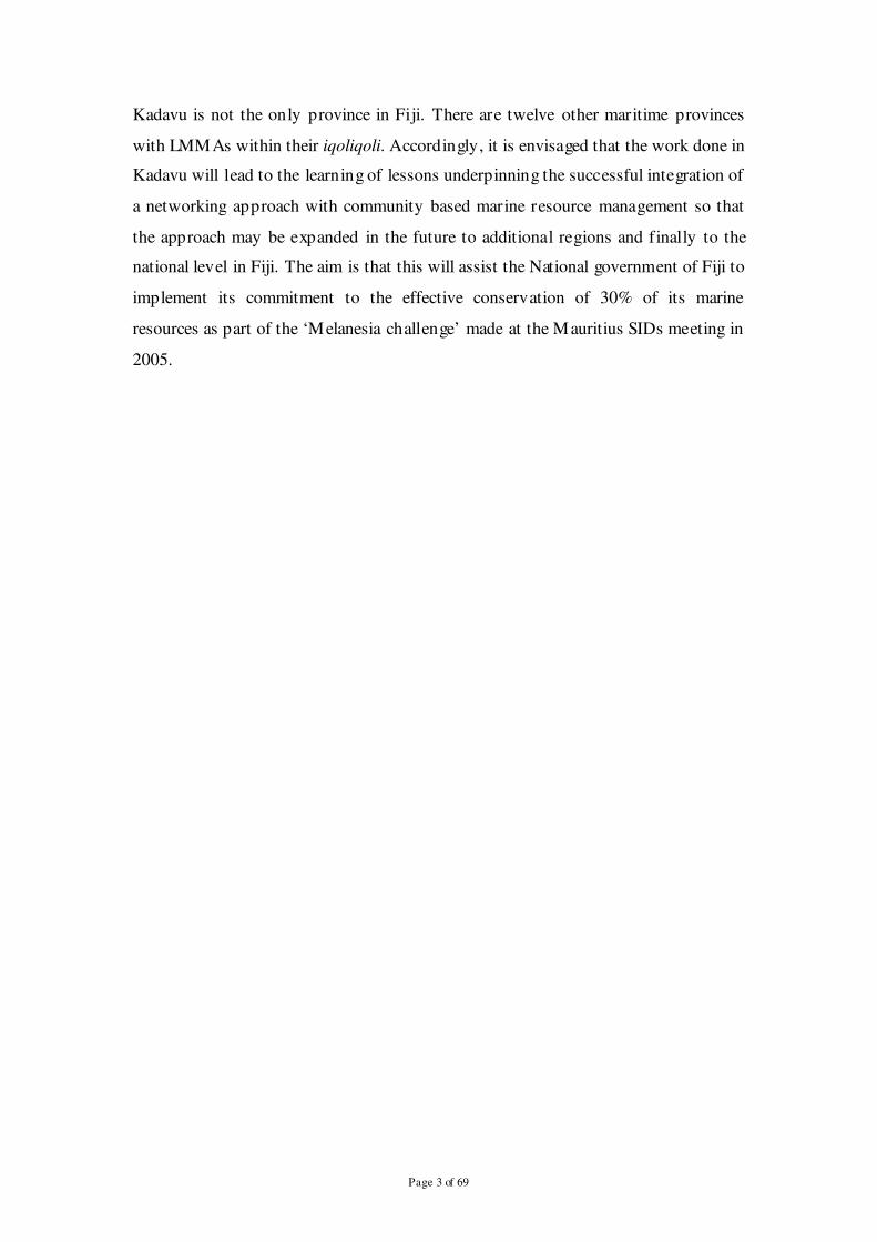
Table 1: IUCN scientific networking criteria for MPAs that were considered for

Kadavu (Reference: IUNC-WCPA 2008)

Criteria Description

Representation a) Need to have all the different types of habitats managed/protected b) Need to protect all different kinds of fish and inverts (maintain the food web - Strength through diversity). c) Should also include ‘special’ places – spawning sites.

Replication Need to have several similar areas protected. Lose one house, need another one to go to.

Resilience and Resistance Protect areas that may be more resistant to bleaching and cyclones (and other hazards – natural or man made).

Ecological significant areas Protect foraging or breeding locations in No-take zones network to ensure that there are enough resources are sustained for future generations. Protection of important sites for reproduction (spawning areas, egg sources).

Ecological linkages Need to have areas that are big enough to protect the fish and inverts home area. Need to have areas of seeding and spill-over, eggs, babies, and adults.

Maintain long-term protection No-take zones should include some permanent sites, if possible.

Maximum contribution of individual no-take zone to the network

It is important to consider size, spacing and shape that allow maximum contribution of individual MPAs to the overall network.

of 69

2.2 Habitat characterization and mapping

Mapping work was done in partnership with the Center for Spatial Environmental

Research (CSER) (http://www.gpem.uq.edu.au/cser)

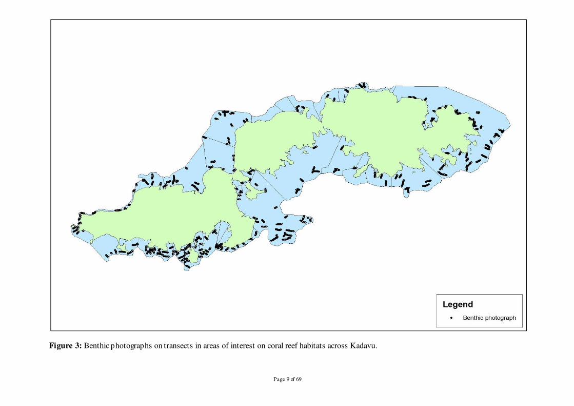
2.2.1 Collection of ground - truthing field data

Field assessment was conducted in two periods; one in June-July and one in October-

November 2009 to collect GPS-photo linked photographs of the coral reef habitats.

Areas of spatially heterogeneous habitats had previously been identified from satellite

imagery and these areas received special attention.

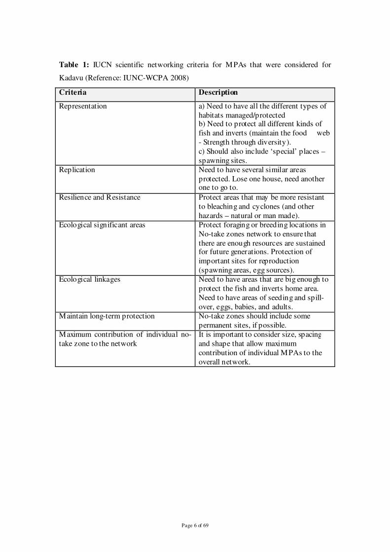
Using this reference guide of marine resource habitat types for Kadavu, extensive

fieldwork around the is land were undertaken to collect photos from identified areas of

interest. Each station of interest was found using a handheld GPS and swam on

compass bearing from GPS start (one station) to end point (another station) using

snorkeling gear. Photos of benthic habitats were taken after each 5 fin kicks using an

Olympus and Canon cameras at 5 mega pixel resolution (figure 2). A total of 211

transects were surveyed where 8,143 georeferenced photographs of the reef

communities were taken in these periods covering all areas around the island.

of 69

Figure 2: Field data collection method and interpretations (source Roelfsema)

Using GPS-Photo Link software (version 4.3.0 GIS Pro) photographs were linked to

the GPS and overlaid onto the satellite imagery together with the GPS coordinates of

where the photos were taken. The software downloaded the photos from the camera

and the GPS tracklog from the GPS receiver and matched the timestamp from the

photo to the closest timestamp in the GPS. The output shape file was named

according to the date the photos were taken, the iqoliqoliID and the camera used

(date_iqoliqoliid_camera).

Transect line, every dot is a position fix

Scuba or snorkelled

transect

of 69

Figure 3: Benthic photographs on transects in areas of interest on coral reef habitats across Kadavu.

of 69

2.2.2 Classifying field data

Collected field data were classified through visual interpretation in Coral Point Count

with Excel extensions (CPCe) using a developed hierarchical classification scheme

(figure 4) for the coral reefs of Kadavu to identify the percentage cover of benthic

habitats around the whole coral reef areas of Kadavu. The scheme included both

geomorphological and ecological features in the definition of the habitat classes. It

was developed by examining schemes previously made for other coastal tropical

regions and adapted to meet shallow water marine ecosystem environment

characteristics.

Habitat types were defined by the geomorphological zone and the predominant

benthic structure or biological cover. The scheme included unconsolidated (e.g. sand

and mud) and consolidated habitats (eg. bedrock and rubble) with the percent cover of

the dominant substrate identified as shown in figure 4. This task was carried out at the

end of the field work period where images were analyzed for the benthic community

and assigned to one of the mapping categories.

of 69

Figure 4: Kadavu classification scheme used for this project

of 69

2.2.3 Image data

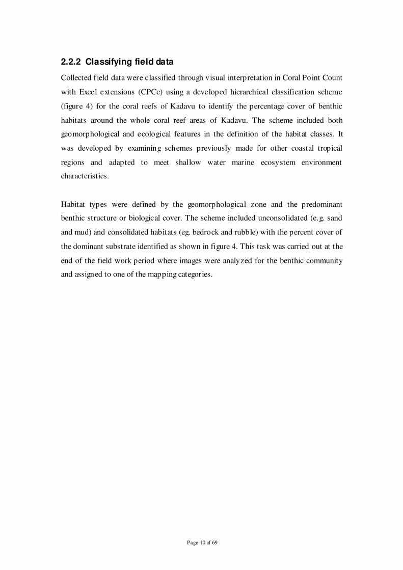
High resolution satellite imagery (figure 5) was acquired covering all of the fishing

grounds and land areas of Kadavu. The satellite imagery used was a composite of

archived Ikonos (4 m pixels) and Quickbird (2.4 m pixels) satellite imagery. The

satellite image data sets were corrected for radiometric and atmospheric distortions to

at-surface reflectance (Phinn et al. in press). A mosaic of Quickbird and Ikonos

images dated from September 2003 to June 2005 were selected to give the least cloud-

affected coverage.

2.2.4 Creating habitat maps

Using Definiens Developer 7.0, four hierarchical spatial scales of habitat maps for the

study site were created based on object based image analysis (Roelfsema et al. 2010).

There were two steps in object based image analysis: 1) image segmentation and 2)

image segment classification (Blaschke 2010). The first step was applied initially on

the whole mosaic image. The segments for a required spatial scale were determined

by this image segmentation step depending on the colour and shape of groups of

pixels and the spatial resolution of mapped features. Later sub-segmentation was

applied on mapping categories of higher level map scale. The second step used

membership rules to manually or automatically assign mapping categories to the

segments. This included the segment: colour, shape, texture, position or biophysical

properties and basically repeated for each of the mapping scales. The membership

rules for this study were developed from previously developed rule sets (Phinn et al.

in press) which mostly required thresholds adjustments for a similar reef type,

geomorphic zone or benthic community mapping category (Roelfsema et al. 2010).

For the first three mapping scales, the segmentation scales and membership rule sets

were mostly determined by image interpretation and expert knowledge whereas the

benthic community scale was mostly based on field data (Roelfsema et al. 2010).

of 69

Figure 5: Mosaic of Quickbird and Ikonos images dated from September 2003 to June 2005

of 69

2.2.5 Accuracy assessment of habitat maps

To assess for accuracy assessment of the habitat maps produced at geomorphic and

benthic community scale, error matrixes were determined. These error matrixes were

based on classified image and reference data for the individual maps and they were

used to calculate commonly used: 1) map accuracy, 2) Overall and Kappa, and 3) the

mapping category accuracies, user and producer (Congalton and Green 1999). Based

on expert knowledge, the geomorphic reference dataset was extracted by manually

assigning geomorphic mapping category to randomly distributed points within each

geomorphic zone. On the other hand, the benthic community reference dataset was

derived from field data set not used for calibration by comparing the filed data with

the underlying segment from the benthic community scale map (Roelfsema et al.

2010).

2.2.6 Final habitat map for Kadavu

The final shapefile of the habitat map produced by the Center for Spatial

Environmental Research (CSER) was further categorized to reflect the CCMA-

NOAA shallow water benthic habitats for the Republic of Palau

(http://ccma.nos.noaa.gov/products/biogeography/palau/htm/refer.html). The

classification scheme for Palau was adopted because the reef system was similar to

that of the project site; Kadavu and the class names used were simple. The mapping

scales were further divided into three habitat categories: 1) NOAA zone, 2) NOAA

structure and 3) NOAA cover. The first category included identified zones from land

to open ocean corresponding to a coral reef geomorphology. These zones included:

intertidal, lagoon, back reef, reef flat, reef crest, fore reef, bank, channel, unknown,

and land. The second category included geomorphological structures that could be

mapped and these included: individual patch reef, aggregated patch reef, aggregate

reef, scattered coral/rock in unconsolidated sediment, pavement, reef rubble,

unconsolidated sand, unconsolidated mud and unknown. The biological cover

category included: coral, seagrass, coralline algae, emergent vegetation, uncolonized,

and unknown.

of 69

The cover types were defined in a collapsible hierarchy ranging from six major

classes (coral, seagrass, coralline algae, emergent vegetation, uncolonized, and

unknown), (figure 6) combined with a density modifier representing the percentage of

the predominate cover type (10% - <50% sparse, 50% - <90% patchy, 90% - 100%

continuous). Substrates not covered with a minimum of 10% of any of the live

biological cover types are classified as uncolonized. Unknown areas included data

that could not be interrupted due to turbidity, cloud cover, water depth, or other

interference.

of 69

Figure 6: Benthic habitat map of Kadavu Island

of 69

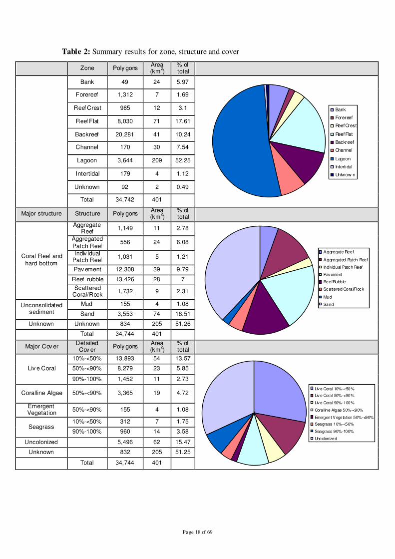
There were 6 major and 9 detailed biological covers, 3 major and 9 distinct structures

and 9 exclusive zones identified across the entire iqoliqoli and mapped in GIS.

Tables 2 shows the summary results of habitat mapping classes used for this study.

For instance, live corals were dominated by sparse corals which covered an area of 54

km2 and this equals 28% of known habitat types. Coralline algae covered an area of

19 km2 whereas emergent vegetation (mangroves) covered 4 km

2 along the intertidal

zone of the main island. The largest area of major structures was constituted by sand

and unconsolidated sediment occupying 74 km2. For coral reef and hard bottom

structures, pavement covered the biggest area across all iqoliqolis (39 km2) whereas

lagoons covered the biggest zone with an area of 209 km2.

of 69

Table 2: Summary results for zone, structure and cover

Zone Poly gons Area (km

2)

% of total

Bank 49 24 5.97

Bank

Forereef

Reef Crest

Reef Flat

Backreef

Channel

Lagoon

Intertidal

Unknow n

Forereef 1,312 7 1.69

Reef Crest 985 12 3.1

Reef Flat 8,030 71 17.61

Backreef 20,281 41 10.24

Channel 170 30 7.54

Lagoon 3,644 209 52.25

Intertidal 179 4 1.12

Unknown 92 2 0.49

Total 34,742 401

Major structure Structure Poly gons Area (km

2)

% of total

Coral Reef and

hard bottom

Aggregate Reef

1,149 11 2.78

Aggregate Reef

Aggregated Patch Reef

Individual Patch Reef

Pavement

ReefRubble

Scattered Coral/Rock

Mud

Sand

Aggregated

Patch Reef 556 24 6.08

Indiv idual Patch Reef

1,031 5 1.21

Pav ement 12,308 39 9.79

Reef rubble 13,426 28 7

Scattered Coral/Rock

1,732 9 2.31

Unconsolidated sediment

Mud 155 4 1.08

Sand 3,553 74 18.51

Unknown Unknown 834 205 51.26

Total 34,744 401

Major Cov er Detailed Cov er

Poly gons Area (km

2)

% of total

Liv e Coral

10%-<50% 13,893 54 13.57

Liv e Coral 10%-<50%

Liv e Coral 50%-<90%

Liv e Coral 90%-100%

Coralline Algae 50%-<90%

Emergent Vegetation 50%-<90%

Seagrass 10%-<50%

Seagrass 90%-100%

Unc olonized

50%-<90% 8,279 23 5.85

90%-100% 1,452 11 2.73

Coralline Algae 50%-<90% 3,365 19 4.72

Emergent Vegetation

50%-<90% 155 4 1.08

Seagrass 10%-<50% 312 7 1.75

90%-100% 960 14 3.58

Uncolonized 5,496 62 15.47

Unknown 832 205 51.25

Total 34,744 401

of 69

2.3 Reserve design planning

The Hexgen command within TNC Protected Area Tools (PAT) v. 2.1 was used to

create a layer of hexagonal Planning Units (PUs) covering the entire inshore fishing

ground areas of Kadavu. The planning units were 1.5 hectares in area and a total of

29,728 were needed to cover the design area.

2.4 Mapping socio-cultural variables and resource use

pattern

One day workshops were conducted in 8 districts around the main island of Kadavu

with invited key representatives from each district to gather information on marine

resource use and traditional knowledge. The workshops used participatory mapping

techniques. The maximum number of attendees per district workshop was 25

including different stakeholder groups based on the following criteria:

• 3 chiefs from villages within the district

• 3 representatives from District Environment Committees • 3 village headman from the district

• 3 village fishermen from the district

• 2 commercial fishermen from the district • 2 members of the KYMST from that district

• 3 community representatives who conduct biological monitoring

• 3 iqoliqoli owners • 3 fisherwomen representatives

of 69

Figure 7: Socio-cultural and resource-use patterns mapping workshop

The workshops covered a wide range of age groups (including elders and chiefs) and

focused on both former and current marine resource users.

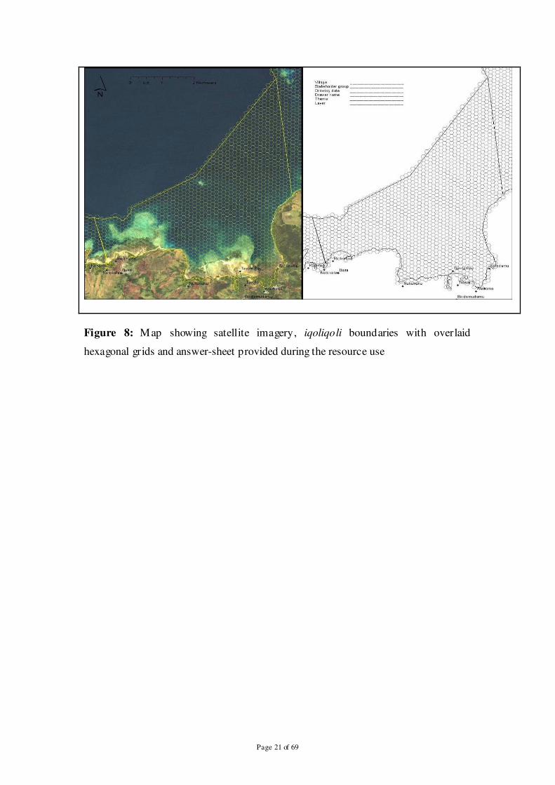
During the workshop, four copies of A2 size laminated maps showing satellite

imagery, iqoliqoli boundaries and planning units were provided to participants. An A4

response-sheet showing the iqoliqoli boundaries, coastline and planning units was

provided in black and white format to record the response of participants.

of 69

Figure 8: Map showing satellite imagery, iqoliqoli boundaries with overlaid

hexagonal grids and answer-sheet provided during the resource use

of 69

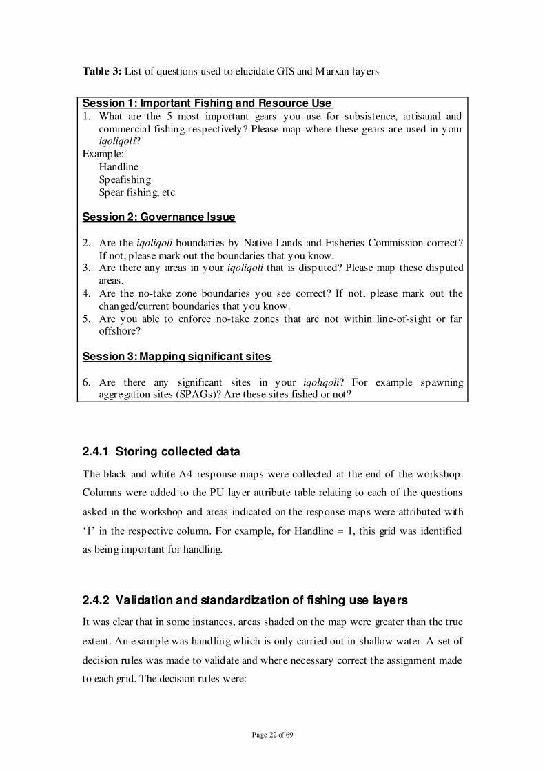
Table 3: List of questions used to elucidate GIS and Marxan layers

Session 1: Important Fishing and Resource Use 1. What are the 5 most important gears you use for subsistence, artisanal and

commercial fishing respectively? Please map where these gears are used in your iqoliqoli?

Example: Handline Speafishing Spear fishing, etc

Session 2: Governance Issue 2. Are the iqoliqoli boundaries by Native Lands and Fisheries Commission correct?

If not, please mark out the boundaries that you know. 3. Are there any areas in your iqoliqoli that is disputed? Please map these disputed

areas. 4. Are the no-take zone boundaries you see correct? If not, please mark out the

changed/current boundaries that you know. 5. Are you able to enforce no-take zones that are not within line-of-sight or far

offshore? Session 3: Mapping significant sites

6. Are there any significant sites in your iqoliqoli? For example spawning aggregation sites (SPAGs)? Are these sites fished or not?

2.4.1 Storing collected data

The black and white A4 response maps were collected at the end of the workshop.

Columns were added to the PU layer attribute table relating to each of the questions

asked in the workshop and areas indicated on the response maps were attributed with

‘1’ in the respective column. For example, for Handline = 1, this grid was identified

as being important for handling.

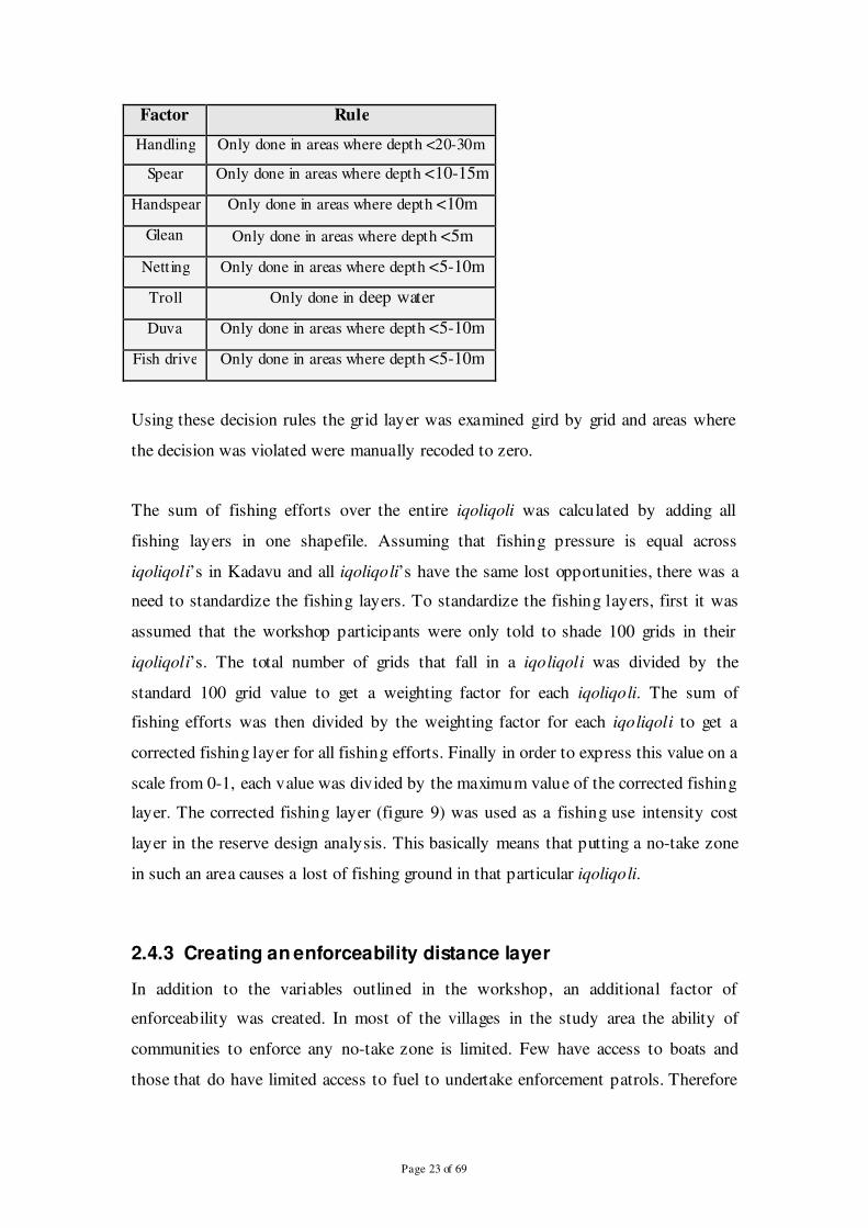
2.4.2 Validation and standardization of fishing use layers

It was clear that in some instances, areas shaded on the map were greater than the true

extent. An example was handling which is only carried out in shallow water. A set of

decision rules was made to validate and where necessary correct the assignment made

to each grid. The decision rules were:

of 69

Factor Rule

Handling Only done in areas where depth <20-30m

Spear Only done in areas where depth <10-15m

Handspear Only done in areas where depth <10m

Glean Only done in areas where depth <5m

Netting Only done in areas where depth <5-10m

Troll Only done in deep water

Duva Only done in areas where depth <5-10m

Fish drive Only done in areas where depth <5-10m

Using these decision rules the grid layer was examined gird by grid and areas where

the decision was violated were manually recoded to zero.

The sum of fishing efforts over the entire iqoliqoli was calculated by adding all

fishing layers in one shapefile. Assuming that fishing pressure is equal across

iqoliqoli’s in Kadavu and all iqoliqoli’s have the same lost opportunities, there was a

need to standardize the fishing layers. To standardize the fishing layers, first it was

assumed that the workshop participants were only told to shade 100 grids in their

iqoliqoli’s. The total number of grids that fall in a iqoliqoli was divided by the

standard 100 grid value to get a weighting factor for each iqoliqoli. The sum of

fishing efforts was then divided by the weighting factor for each iqoliqoli to get a

corrected fishing layer for all fishing efforts. Finally in order to express this value on a

scale from 0-1, each value was divided by the maximum value of the corrected fishing

layer. The corrected fishing layer (figure 9) was used as a fishing use intensity cost

layer in the reserve design analysis. This basically means that putting a no-take zone

in such an area causes a lost of fishing ground in that particular iqoliqoli.

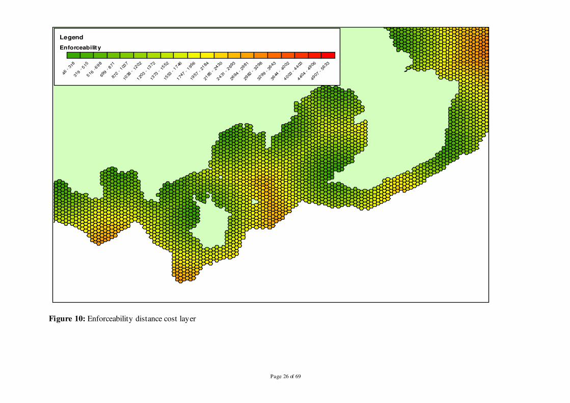
2.4.3 Creating an enforceability distance layer

In addition to the variables outlined in the workshop, an additional factor of

enforceability was created. In most of the villages in the study area the ability of

communities to enforce any no-take zone is limited. Few have access to boats and

those that do have limited access to fuel to undertake enforcement patrols. Therefore

of 69

it is important that any no-take area be established within a relatively short distance

from the village and certainly within line-of-sight.

In order to create this layer, a ‘straight line’ analysis using ArcGIS Spatial Analysis

was undertaken to assign a distance of each PU from the nearest village (figure 10).

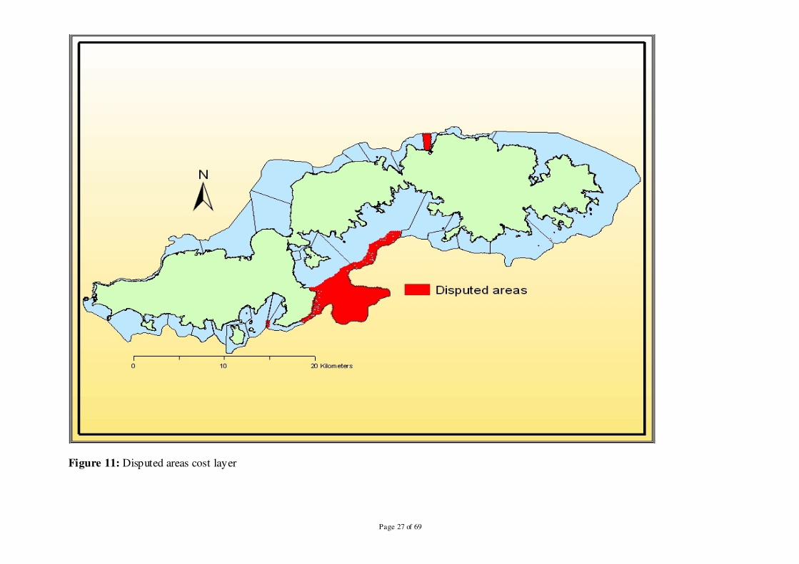
2.4.4 Creating a disputed areas layer

Disputed areas included areas of iqoliqoli where there have been disputes over the

years regarding traditional ownership (figure 11). The communities identified these

areas at the resource use and traditional knowledge workshop. The identified areas

were spatially recorded in GIS and the areas were calculated in square meters to be

used as disputed areas layer in the analysis.

of 69

Figure 9: Fishing use intensity cost layer

of 69

Legend

Enforceability

46 -

31

83

19 -

51

55

16 -

69

86

99 -

87

187

2 - 1

037

10

38 -

12

021

203

- 1

372

13

73 -

15

521

553

- 1

746

17

47 -

19

561

957

- 2

184

21

85 -

24

302

431

- 2

693

26

94 -

29

812

982

- 3

298

32

99 -

36

433

644

- 4

002

40

03 -

44

034

404

- 4

906

49

07 -

56

33

Figure 10: Enforceability distance cost layer

of 69

Figure 11: Disputed areas cost layer

of 69

2.5 Assessment of the pre-existing network and gap

analysis

The pre-existing no-take zone network as of December 2010 included 60 individual

community-based no-take zones (figure 12). The network protected a total area of

29.4 km2 (12%) of shallow reefs areas and 0.5 km

2 (17%) of significant sites across

the network.

Using the IUCN stated MPA networking principles, habitat maps and the community

resource use maps, a feasibility assessment was undertaken to assess which pre-

existing no-take zones fulfil the network design principles and which do not fulfil

some or all of these principles.

2.5.1 Representation

There are two ways in which representation of habitats within the existing no-take

zone network were assessed.

Percentage habitat representation per no-take zone area and across the network

To quantify the habitat coverage in each no-take zone, the spatial join performed

previously and the calculated areas of each habitat polygon was used to calculate the

area of each habitat type within each no-take zone. After performing no-take zone

specific calculations it was then possible to sum habitat areas across all no-take zones

and therefore calculate the percent representation of each habitat within the no-take

zone network.

Diversity of habitats within each no-take zone

To assess the number of distinct habitat types in each no-take zone a spatial join

between the habitat maps and the no-take zone boundaries was created. Using this

spatial join allows for the number of distinct habitat types present in each no-take

zone to be enumerated.

of 69

Figure 12: Pre-existing no-take zone as a network around the island of Kadavu.

of 69

Habitat complexities

The number of distinct habitat patches in each no-take zone was first assessed using a

spatial join between the habitat map and the no-take zone boundaries were created.

Using this spatial join allows for the number of distinct habitat types present in each

no-take zone to be enumerated. This was then later compared across all no-take zones

in the pre-existing network.

2.5.2 Replication

To assess replication of habitats within the existing no-take zone network, the

different habitat types present in each no-take zone were identified and labelled. After

performing no-take zone specific enumerations it was then possible to calculate the

number of no-take zone within the network where these distinct habitat types exist.

The number of no-take zone that covers the major habitats for managing and

protecting fish and invertebrates were also noted.

Significant sites such as spawning aggregation sites, cultural areas and turtle nesting

sites were also assessed against representation and replication networking principles.

Table 4 shows the percent of each feature (zone, habitat, significant sites) around

Kadavu that is already protected by no-take zone. It also shows the number of no-take

zone each feature occurs in (replication) and the number of distinct habitat patches

protected by no-take zones.

of 69

Table 4: Feature representation, occurrence and number of habitat patches across the

re-designed network on Kadavu before the project

Feature % protected

% (number) of no-take zone s in which feature

occurs in

Number of patches protected

Geomorphic zone

Back reef 2 5 (3) 279

Channel 8 23 (14) 21

Fore reef 5 17 (10) 39

Intertidal 15 20 (12) 21

Lagoon 13 50 (30) 569

Reef crest 5 13 (8) 63

Reef flat 18 97 (58) 1,344

Habitat

Continuous coral 12 60 (36) 268

Patchy coral 12 77 (46) 570

Sparse coral 6 57 (34) 272

Dense seagrass 16 53 (32) 187

Sparse seagrass 15 42 (25) 53

Patchy coralline 6 27 (16) 148

Patchy vegetation 16 18 (11) 19

Significant sites

Spawning aggregations sites

41 12 (7)

Turtle nesting sites 24 3 (2)

Cultural areas 7 15 (9)

These results (Table 4) showed that the most represented and replicated

geomorphological zone in the pre-existing network was reef flat. It had the highest

percent protected with 18% in no-take zones and the most occurred feature across the

network in 58 (97%) no-take zones. Reef flat patches were also the most protected

with 1,344 of them in no-take zones across the network. In addition intertidal zone

was the second most protected class with 15% in no-take zones. This however was

replicated in only 12 (20%) no-take zones with 21 patches protected, the least across

the network. Half the no-take zones had lagoon within them; representing 13% of the

total lagoon area and 569 lagoon patches. The network was also protecting 8% of

channel, 5% of reef crest and fore reef areas. Back reef was the geomorphological

zone that was least protected with only 2% in no-take zones occurring in 3 no-take

zones.

The fact that communities put more no-take zones in reef flat and intertidal zones

were evident in the high percent of seagrass and mangrove vegetation habitat

of 69

protected. Table 4 shows that patchy vegetation and dense seagrass habitat was the

most protected habitat feature with 16% of dense and 15% of sparse seagrass in no-

take zone. Dense seagrass was replicated in over 50 no-take zones; patchy vegetation

however was replicated in only 11 (18%) no-take zones. There were only 19 patches

of patchy vegetation protected in this case whereas over 150 patches of dense seagrass

were protected. In addition the network also protected 12% of continuous coral and

12% patchy corals in no-take zones with patchy coral being the most replicated

feature in 46 no-take zones and most number of patches protected with 570 of them in

no-take zones. Patchy coralline algae and sparse coral were the least protected habitat

with only 6% in no-take zones.

Community significant sites were also found to be protected by the pre-existing

network when assessed. It was protecting 41% of spawning aggregation (SPAGs),

which was replicated in 7 no-take zones (Table 4). The network also protected 24% of

turtle nesting sites in 2 no-take zones and 7% of culturally important areas were

protected by 9 no-take zones in the network.

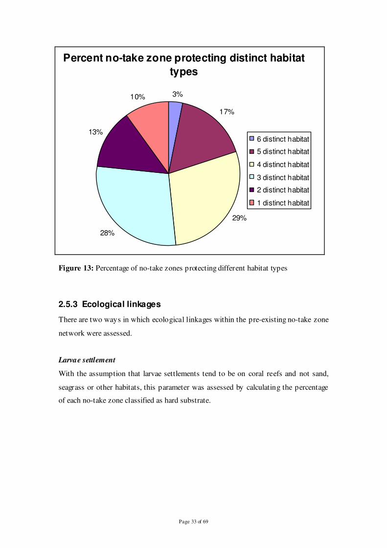
When pre-existing network was assessed against habitat diversity, 7 distinct habitat

types had been protected across Kadavu. Figure 13 shows the percentage of no-take

zones and the number of distinct habitat types they protect. Diversity of habitats

within pre-existing no-take zones ranged from one to six distinct habitats per no-take

zone. Most no-take zones protected four to five distinct habitat types across the pre-

existing network. Only 3% of no-take zones protected six out of seven distinct habitat

types whereas 10% of no-take zones protected one habitat type.

of 69

Percent no-take zone protecting distinct habitat

types

3%

17%

29%

28%

13%

10%

6 distinct habitat

5 distinct habitat

4 distinct habitat

3 distinct habitat

2 distinct habitat

1 distinct habitat

Figure 13: Percentage of no-take zones protecting different habitat types

2.5.3 Ecological linkages

There are two ways in which ecological linkages within the pre-existing no-take zone

network were assessed.

Larvae settlement

With the assumption that larvae settlements tend to be on coral reefs and not sand,

seagrass or other habitats, this parameter was assessed by calculating the percentage

of each no-take zone classified as hard substrate.

of 69

0

5

10

15

20

25

30

35

40

Continuous

coral

Patchy coral Patchy

coralline

Sparse coral Total

Hard substrate features

% in

clu

sio

n in

no-t

ake z

one

pre-exis ting network

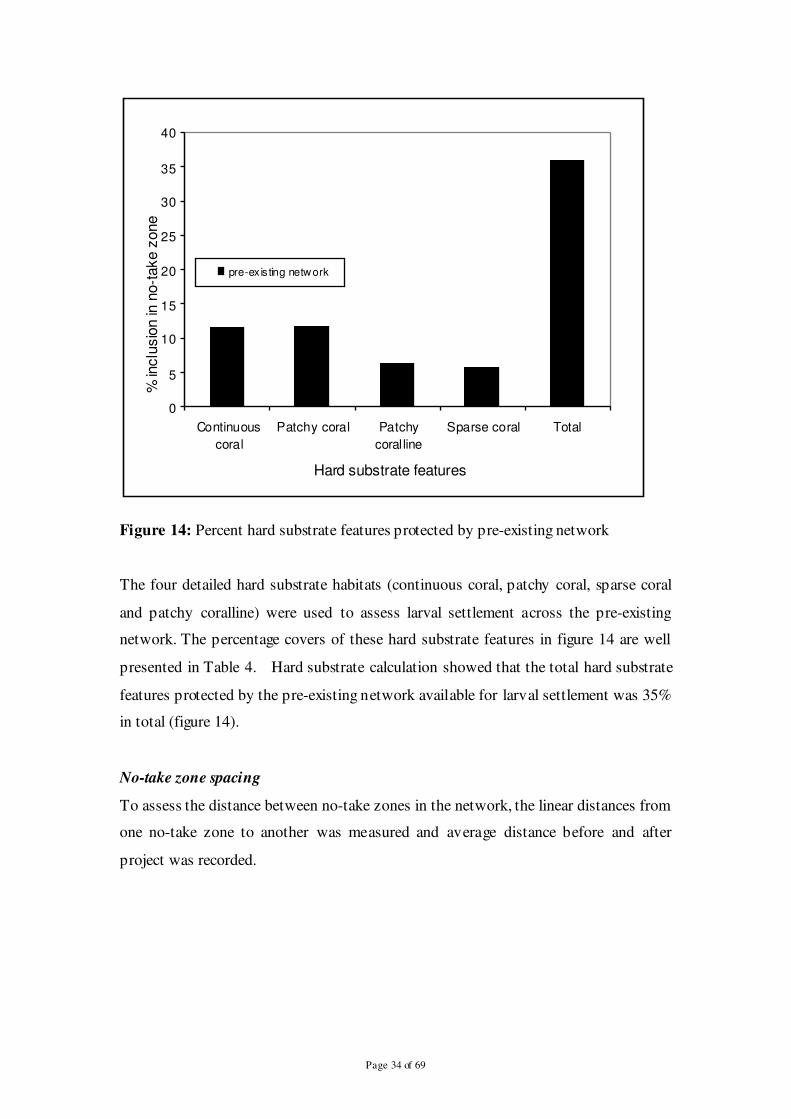
Figure 14: Percent hard substrate features protected by pre-existing network

The four detailed hard substrate habitats (continuous coral, patchy coral, sparse coral

and patchy coralline) were used to assess larval settlement across the pre-existing

network. The percentage covers of these hard substrate features in figure 14 are well

presented in Table 4. Hard substrate calculation showed that the total hard substrate

features protected by the pre-existing network available for larval settlement was 35%

in total (figure 14).

No-take zone spacing

To assess the distance between no-take zones in the network, the linear distances from

one no-take zone to another was measured and average distance before and after

project was recorded.

of 69

Table 5: No-take zone spacing distance in the pre-existing network

Spacing parameter Pre-existing network (meters)

Maximum spacing distance 10,456 m

Minimum spacing distance 329 m

Average spacing distance 3,131 m

The maximum spacing distance between no-take zones in the pre-existing network

before the project was 10,456 meters and the minimum spacing distance was 329

meters. The average spacing distance between no-take zones was 3,131 meters (Table

5).

2.5.4 Long - term protection

Years in existence

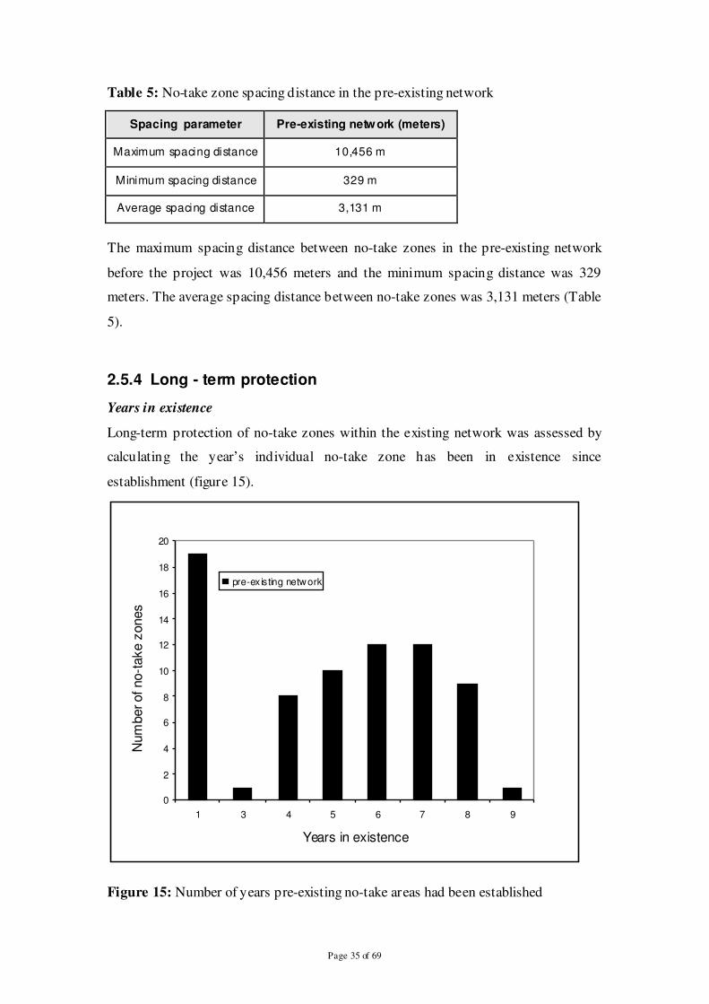
Long-term protection of no-take zones within the existing network was assessed by

calculating the year’s individual no-take zone has been in existence since

establishment (figure 15).

0

2

4

6

8

10

12

14

16

18

20

1 3 4 5 6 7 8 9

Years in existence

Num

ber of no-t

ake z

ones

pre-ex is ting network

Figure 15: Number of years pre-existing no-take areas had been established

of 69

The pre-existing network included no-take zones that were initiated between the 2001

and 2009. The average age of the existing no-takes was 4.6 years. Across the network,

only a single no-take zone had been in existence for nine years (initiated in 2001).

Figure 15 shows that nineteen no-take zones had been in existence for just 1 year

(initiated in 2009). Nine no-take zones were 8 years old and twelve no-take zones

were established in the 2003 and twelve in 2004 which were 7 and 6 years in

existence respectively. Ten no-take zones were 5 years old and 8 were four years on

the ground. On average, the network had been 4 years in existence.

2.5.5 Maximising the contribution of individual no-take zones to

the overall network

To assess if the contribution of individual no-take zone to the current network is

maximised, the size of the no-take zones were calculated and compared to the home

range of Lethrinidae fish family, one that is commonly used by communities in Fiji.

The size was calculated by using a spatial tool in GIS to find out the maximum

dimension of no-take zones.

Recent studies done in the Coral Coast of Fiji and funded by NOAA showed that the

average movement of Lethrinidae fish was less than 900 meters. For this the numbers

of no-take zones that have their size greater than 900 meters were recorded.

of 69

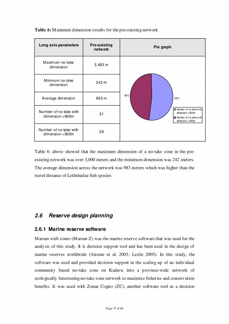
Table 6: Maximum dimension results for the pre-existing network

Long axis parameters

Pre-existing

network

Pie graph

Maximum no-take

dimension

3,493 m

52%48%

Number of no- take w ith

dimension >900m


dimension <900m

Minimum no-take dimension

242 m

Average dimension

983 m

Number of no-take with

dimension >900m

31

Number of no-take with dimension <900m

29

Table 6: above showed that the maximum dimension of a no-take zone in the pre-

existing network was over 3,000 meters and the minimum dimension was 242 meters.

The average dimension across the network was 983 meters which was higher than the

travel distance of Lethrinidae fish species.

2.6 Reserve design planning

2.6.1 Marine reserve software

Marxan with zones (Marxan Z) was the marine reserve software that was used for the

analysis of this study. It is decision support tool and has been used in the design of

marine reserves worldwide (Airame et al. 2003; Leslie 2005). In this study, the

software was used and provided decision support in the scaling up of an individual

community based no-take zone on Kadavu into a province-wide network of

ecologically functioning no-take zone network to maximize fisheries and conservation

benefits. It was used with Zonae Cogito (ZC), another software tool as a decision

of 69

support system and database management system for Marxan software. GIS software

components were also integrated in ZC which makes work easier. The design of ZC is

simple and strong making it easier to run Marxan analyses and viewing the results

after each analysis.

For further information, please consult the Marxan with Zones manual v1.0.1 (Watts

et al. 2008) and more information can be found at

http://www.uq.edu.au/marxan/zonae-cogito-software.

2.6.2 Assembling primary input files

Once the GIS data layers had been created, the next step was to create input files

needed for Marxan with Zones analysis. These input data files were created using

ArcGIS, Jump statistical software, Microsoft Excel and Access. There were seven

fundamental input files that were required to run Marxan. In addition, there are

optional files that facilitate additional function.

of 69

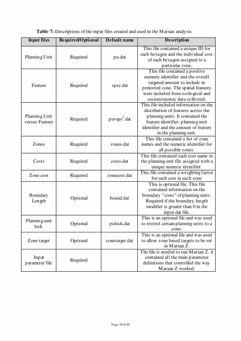
Table 7: Descriptions of the input files created and used in the Marxan analysis

Input files Required/Optional Default name Description

Planning Unit Required pu.dat

This file contained a unique ID for each hexagon and the individual cost

of each hexagon assigned to a particular zone.

Feature Required spec.dat

This file contained a positive numeric identifier and the overall

targeted amount to include in protected zone. The spatial features were included from ecological and

socioeconomic data collected.

Planning Unit versus Feature

Required puvspr2.dat

This file included information on the distribution of features across the

planning units. It contained the feature identifier, planning unit

identifier and the amount of feature in the planning unit.

Zones Required zones.dat This file contained a list of zone

names and the numeric identifier for all possible zones.

Costs Required costs.dat This file contained each cost name in the planning unit file assigned with a

unique numeric identifier.

Zone cost Required zonecost.dat This file contained a weighting factor

for each cost in each zone

Boundary Length

Optional bound.dat

This is optional file. This file contained information on the

boundary “costs” of planning units. Required if the boundary length modifier is greater than 0 in the

input.dat file.

Planning unit lock

Optional pulock.dat This is an optional file and was used to restrict certain planning units to a

zone.

Zone target Optional zonetarget.dat This is an optional file and was used to allow zone based targets to be set

in Marxan Z.

Input parameter file

Required

The file is needed to run Marxan Z. it contained all the main parameter

definitions that controlled the way Marxan Z worked.

of 69

2.6.3 Community targets

To protect 30% of each habitat features and 100% of significant sites (Spawning

Aggregations, cultural sites and turtle nesting areas).

2.6.4 Conservation features

The conservation and fisheries targets represented the spatial distribution of the major

biodiversity features that were considered. Conservation feature targets included:

o Continuous coral reef habitat types based on field assessment survey (2009)

and habitat map produced by UQ (2010).

o Patchy coral reef habitat types based on field assessment survey (2009) and

habitat map produced by UQ (2010).

o Sparse coral reef habitat types based on field assessment survey (2009) and

habitat map produced by UQ (2010).

o Patchy coralline red algae habitat types based on based on field assessment

survey (2009) and habitat map produced by UQ (2010).

o Dense seagrass communities based on field assessment survey based on field

assessment survey (2009) and habitat map produced by UQ (2010).

o Sparse seagrass communities based on field assessment survey based on field

assessment survey (2009) and habitat map produced by UQ (2010).

o Patchy emergent vegetations cover (mangroves) based on digitized mangrove

areas on Google image 2010.

o Spawning aggregation sites (SPAGs) based on survey of local traditional

knowledge and resource use in Kadavu (2009).

o Cultural areas based on survey of local traditional knowledge and resource use

in Kadavu (2009).

o Turtle nesting sites based on survey of local traditional knowledge and

resource use in Kadavu (2009).

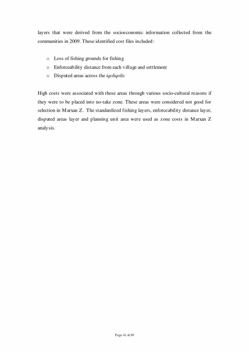
2.6.5 Planning Units and costs

The same hexagonal grids that were created for mapping community resource use and

traditional knowledge were generated as a planning unit (PU) file (Figure15) for

Marxan analysis. The PU file consisted of a number of unique identifiers and the cost

of 69

layers that were derived from the socioeconomic information collected from the

communities in 2009. These identified cost files included:

o Loss of fishing grounds for fishing

o Enforceability distance from each village and settlement

o Disputed areas across the iqoliqolis

High costs were associated with these areas through various socio-cultural reasons if

they were to be placed into no-take zone. These areas were considered not good for

selection in Marxan Z. The standardized fishing layers, enforceability distance layer,

disputed areas layer and planning unit area were used as zone costs in Marxan Z

analysis.

of 69

Figure 16: Marxan planning unit layer.

of 69

2.6.6 Zones

The two zones included in the zones file were zone 1 = fished and zone 2 = no-take

zone. In the zone target file each feature and Iqoliqoli target was set for each zone.

The targets represent major ecological habitats and Iqoliqoli areas that communities

wished to protect or leave them out to fishing.

2.6.7 Planning unit lock

This file was used to restrict certain planning units to a zone. In the analysis, there

were some instances where the pre-existing no-take zone were locked in or restricted

to zone 2 and other runs where the re-designed no-take zones were locked in.

2.6.8 Summary input files

A summary of the input files used for re-designing the no-take zone network are

outlined below:

o Planning unit file “pu.dat” = 29,728 hexagons

o Feature file “spec.dat” = 8 unique habitat features, 29 inshore iqoliqoli

targets, 29 offshore iqoliqoli targets and 3 ecological significant sites

o Zone target “zone target” = 30% habitat features in no-take zone , 60%

inshore reefs of each iqoliqoli in fished and 100% of ecological significant

sites in no-take zone

o Area of each planning unit = 14,997 square meters

o Boundary Length Modifier = 60 (the BLM is a parameter that directs the

assignment of planning units to zones in a cluster formation rather than

selecting several disconnected planning units. BLM 60 provided a

moderate degree of clumping that produced compact areas of similar size

to that of pre-existing no-take zones).

o Penalty Factor = 1,000 (the penalty factor is a measure of the relative

worth of a feature and how important it is to represent that feature. This

was set equally across all conservation targets).

o Annealing Parameters

of 69

� NUMITNS = 10,000,000 (the number of times Marxan with zones

tries to generate a solution for each run).

� NUMREPS = 100 (the number of separate runs with the same

starting condition).

2.6.9 Running Marxan

Zonae Cogito interface was used to run Marxan Z. This made the analysis easier

because of the editable nature of the software and a view of the result after each run.

The Marxan input data files were added into ZC together with a Planning Unit

shapefile for GIS display. In the process the input parameter files were edited

according to the desired targets.

Two Marxan runs were made based on two different scenarios

1. With pre-existing no-take zones locked in- that the contribution already made by the existing no-take zone area is recognized by Marxan and only additional areas to comprise the shortfall between existing protection and the overall target are identified

2. Without pre-existing no-take zones locked in: It was decided early on in the project that as many of the no-take zones have been established for many years, the conservation cost associated with relocating them would be considerable.

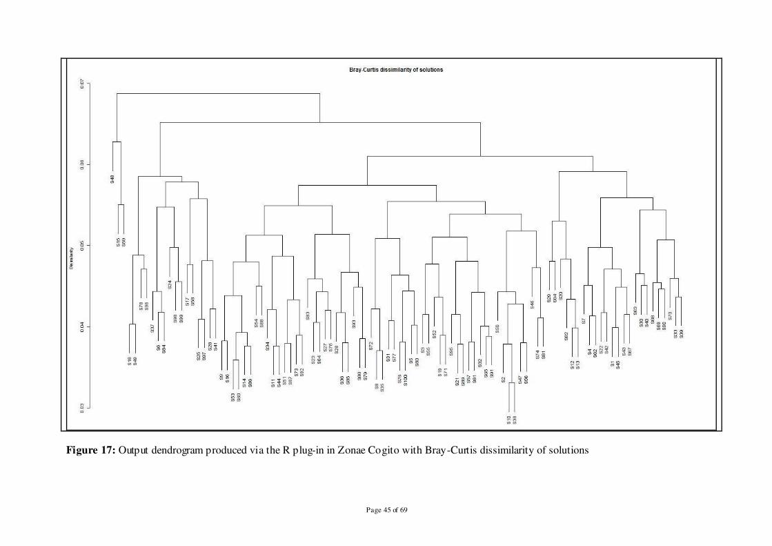
2.6.10 Examining runs

The output dendrogram produced via the R plug-in in Zonae Cogito (Figure 16) was

examined to identify two of the least similar of the total 100 solutions produced.

Solutions 48 and 10 were the least similar; with a Bray-Curtis dissimilarity of 0.068.

This level of dissimilarity is low and suggests that the difference in spatial

configurations of the two most ‘different’ solutions is actually very similar.

In order to examine this, the no-take zone configurations of the two least similar

solutions were overlaid in ArcGIS. 5.6% of the PUs selected as no-take zones in

solution 48 were not selected in solution 10; and 4.3% of PUs selected as no-take

zones in solution 10 were not selected in solution 48.

of 69

Figure 17: Output dendrogram produced via the R plug-in in Zonae Cogito with Bray-Curtis dissimilarity of solutions

of 69

2.7 Supplementing the existing- communicating design

results

Four community level workshops were conducted for the 8 districts on the main

island. Similar criteria to select participants from the initial socio-cultural workshop in

2009 were used including the Chiefs and iqoliqoli owners. The programme of these

workshops is shown below.

Communicating design- workshop programme 9:00 Introduction to workshop � History of project

� Current status of no-take areas � Kadavu process and visioning

� Development of this project � NOAA Kadavu project goals and objectives

10:00 Session 1 � Recap on this project

- how the project started - visioning workshop in 2007

- Introduce MPA and MPA networks - Recap of the fieldwork and data collection processes

- Community feedback

11:30 Session 2

� Present the results back to the communities (to familiarize the communities with the maps)

- Basemap (Current no-take zone and verify them with the communities, discuss where there is still conflict)

- Habitat map (Discuss how habitats fits into existing no-take zone s – network principles)

- Present status of MPAs - % habitat represented in the current

- Community feedback

2:00 Session 3 � Re-Design no-take zone Network First present outlines

- Marxan output (the different scenarios) - Adding to existing - Best Run (Best locked offshore excluded)

- Modify existing - Selection Frequency (No-take zone unlocked-offshore excluded (Present recommended areas to fil l the Gap)

4:00 Session 4: � Moving towards an island-wide network of MPAs

- Did we miss any important considerations - Discussion of influence of governance issue s to NTZ network-obstacles, value,

opportunities - Questions

5:00 Workshop close

of 69

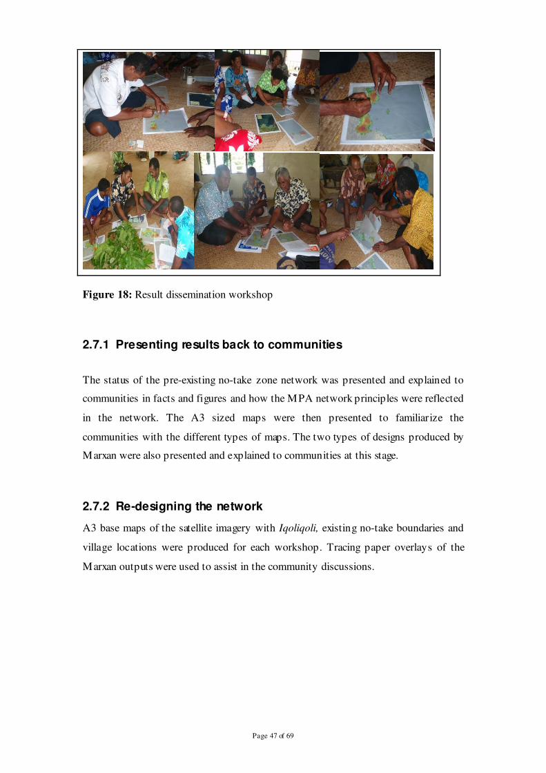
Figure 18: Result dissemination workshop

2.7.1 Presenting results back to communities

The status of the pre-existing no-take zone network was presented and explained to

communities in facts and figures and how the MPA network principles were reflected

in the network. The A3 sized maps were then presented to familiarize the

communities with the different types of maps. The two types of designs produced by

Marxan were also presented and explained to communities at this stage.

2.7.2 Re-designing the network

A3 base maps of the satellite imagery with Iqoliqoli, existing no-take boundaries and

village locations were produced for each workshop. Tracing paper overlays of the

Marxan outputs were used to assist in the community discussions.

of 69

Marxan outputs from two scenarios were used in the workshop: The ‘best’ run (figure 20) output overlay was used from the first scenario in which existing no-take zone areas were locked in The selection frequency (figure 19) overlay was used from the second scenario in which the existing no-take zone areas were not locked in In some instances communities wanted to retain the existing no-take areas, and wished to add additional areas. Where this was the case the best run maps were most frequently used. In other instances, some communities expressed a desire to move the location of the existing no-take areas within their fishing ground. In these cases the selection frequency maps were of most value in identifying ecologically important areas. Some villages that did not have any no-take areas prior to this project used the best run and the selection frequency maps together.

of 69

Figure 19: Marxan selection frequency without pre-existing no-take zones locked in (100 reps).

of 69

Figure 20: Marxan best run solution where pre-existing no-take zone were locked in (100 reps).

of 69

The two outputs above (Figures 19-20) were used to identify areas of interest for

inclusion in the re-designed no-take zone network. Both designs showed important

areas in each iqoliqoli to include in the network and achieve the overall provincial

target of 30% to protect inshore habitats.

The best run design was used where communities wished to add to the pre-existing

no-take zones. The selection frequency was used to modify the existing and to

recommend areas to fill the gap where the best run cannot be used. At the end of the

workshop the communities had re-designed an implemented network of no-take zones

for the province of Kadavu. Maps of the re-designed network were created and sent to

each community in Kadavu.

2.8 The modified network

Of the 60 existing no takes at the start of the project, 35 were not modified, whilst the

remaining 25 were modified in some way (12 had additional areas added to them, 3

shrunk in size, 9 were moved and 1 large area was split into four smaller areas).

In addition, 14 new no-take areas were established through this project.

The total area under no-take zone increased from 29.4 km2 to 50.1 km

2 as a result of

the redesign project. . In addition, the re-designed network now protects an additional

of 1 km2 (38%) of significant sites.

There was an overall increase in protection in the community re-designed network

when compared to the pre-existing network. There was an overall increase of 20.7

km2 in total area protected by the re-designed network. Significant sites also increased

by 21%. The re-designed network is 7% more compacted and the average social cost

was 12.4% less than the pre-existing network. The re-designed network now protects

19% of shallow reef areas. There was an overall increase of 7% in features across

network. Table 8 shows the percent of each feature around all of Kadavu after the

project.

of 69

All modifications have been endorsed at the relevant village meetings and came into

effect on the 1st of March 2011.

of 69

Figure 21: Community re-designed and implemented no-take zones network on Kadavu

of 69

2.8.1 Representation

There was an overall increase in geomorphological zone protected in the community

re-designed network. After assessment, findings were communities had now put more

channels into no-take zones which now resulted in 29% of channel being protected.

This was an increase of 21% from the pre-existing network before the project started.

Reef flat was the zone feature that was the most protected in the previous network and

now protects 26%, an increase in 8%. Although back reef is still the least zone

protected, it now protects 14%. This was a 12% increase from the previous network

which protected only 2%.

The most represented habitat across the re-designed network was seagrass. In fact

sparse seagrass was the only habitat feature target achieved, with 34% now protected

(Table 8). Patchy vegetation and dense seagrass was the second most represented

habitat feature in the re-designed network. There was an increase of 13% in the

proportion of patchy coralline habitat protected from 6% to 19%. Sparse coral was the

least represented habitat in the re-designed network with 15% protected by no-take

zones. In terms of number of patches protected, sparse coral patches were the most

protected with 1,911 was followed by patchy coral with 1,350. Over 700 patchy

coralline patches were also protected however only 19 patches of patchy vegetation

were included in no-take zones.

of 69

Table 8: Feature representation, occurrence and number of habitat patches across the

re-designed network on Kadavu after the project

Feature % protected

% (number) of no-take zone s in which feature

occurs in

Number of patches protected

Geomorphic zone

Back reef 14 6 (5) 2,923

Channel 29 23 (18) 43

Fore reef 16 23 (18) 186

Intertidal 22 21 (16) 38

Lagoon 16 56 (43) 761

Reef crest 16 16 (12) 144

Reef flat 26 92 (71) 1,842

Habitat

Continuous coral 19 62 (48) 414

Patchy coral 20 79 (61) 1,350

Sparse coral 15 58 (45) 1,911

Dense seagrass 23 61 (47) 238

Sparse seagrass 34 36 (28) 82

Patchy coralline 19 27 (21) 743

Patchy vegetation 23 19 (15) 36

Significant sites

Spawning aggregations sites

80 23 (18)

Turtle nesting sites 61 4 (3)

Cultural areas 21 16 (12)

2.8.2 Replication

Table 8 shows the number of no-take zones in which each feature occurs across the

re-designed network. It shows that there was an overall increase in feature occurrence

in no-take zones across the network. For example, reef flat was still the most

replicated zone across the re-designed network. It occurred in over 90% of no-take

zones with 1,842 reef flat patches protected. Back reef on the other hand only

occurred in 5 no-take zones.

Generally live corals were the most replicated habitat feature across the re-designed

network (Table 8). For instance, patchy coral was still the most replicated habitat

feature across the network in 79% of no-take zones, continuous coral being the second

most frequently occurring habitat feature in 62% of no-take zones and sparse coral in

58% no-take zones. Patchy vegetation was the least replicated habitat feature that

occurred in 15 no-take zones.

of 69

Channels were the most protected significant sites across the re-designed network. In

fact, channel was the most protected zone in the re-designed network (Table 8). Of the

100% Spawning Aggregation provincial target set, 80% was protected by the

redesigned network. This was an increase of 38% protection for Spawning

Aggregation sites. Over 60% known turtle nesting sites were also part of the re-

designed network across 3 no-take zones. This was an increase of 37% in turtle

nesting sites from the pre-existing network. Finally 21% cultural areas were included

in 12 no-take zones in the re-designed network, a 13% increase from the 7% cultural

areas protected by the pre-existing network.

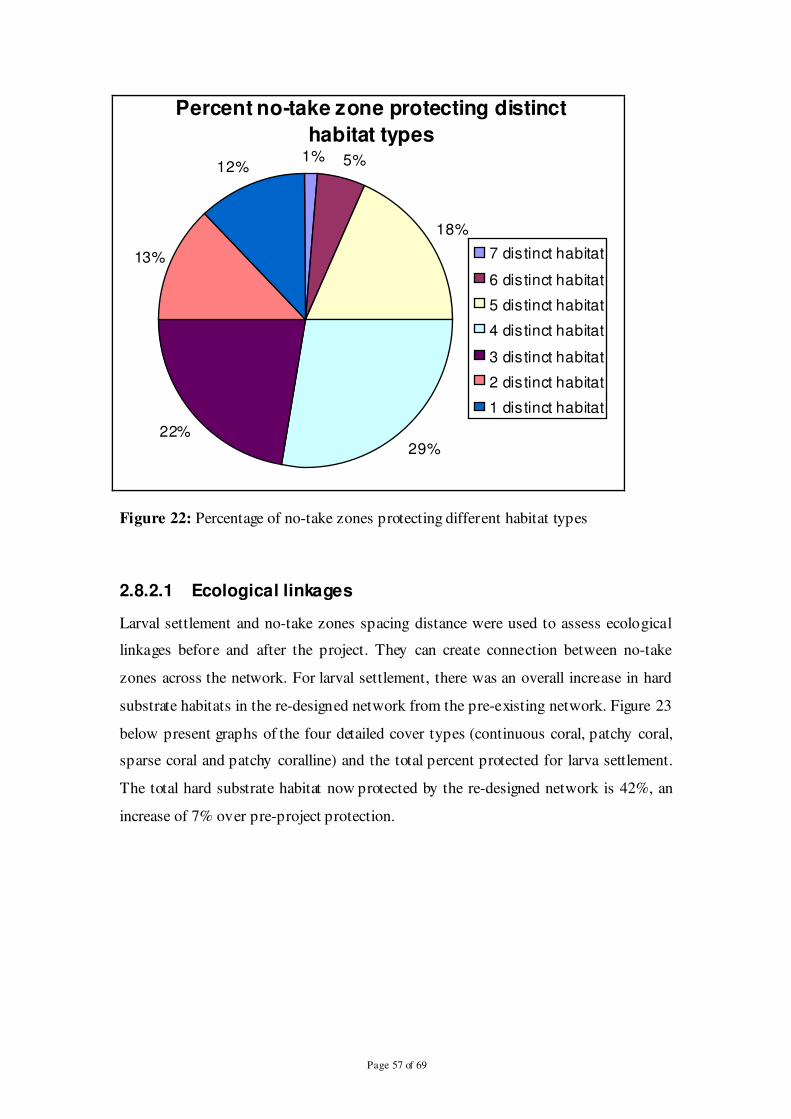
Diversity of habitats across the re-designed network now range from one habitat type

per no-take zone to seven distinct habitats per no-take zone. Figure 22 shows the

percentage of no-take zones and the number of distinct habitat types they protect. Out

of the seven distinct habitat types assessed, only 1% no-take zones protected all

distinct habitat types, 5% of no-take zones protected six distinct habitats and 18% of

no-take zones protected five distinct habitat types across the network. Most no-take

zones (29%) protected four distinct habitat types and 22% of no-take zones protected

three distinct across the network. Two distinct habitat types were protected by 13%

no-take zones and finally one distinct habitat type was protected by 12% no-take

zones.

of 69

Percent no-take zone protecting distinct

habitat types 1% 5%

18%

29%22%

13%

12%

7 distinct habitat

6 distinct habitat

5 distinct habitat

4 distinct habitat

3 distinct habitat

2 distinct habitat

1 distinct habitat

Figure 22: Percentage of no-take zones protecting different habitat types

2.8.2.1 Ecological linkages

Larval settlement and no-take zones spacing distance were used to assess ecological

linkages before and after the project. They can create connection between no-take

zones across the network. For larval settlement, there was an overall increase in hard

substrate habitats in the re-designed network from the pre-existing network. Figure 23

below present graphs of the four detailed cover types (continuous coral, patchy coral,

sparse coral and patchy coralline) and the total percent protected for larva settlement.

The total hard substrate habitat now protected by the re-designed network is 42%, an

increase of 7% over pre-project protection.

of 69

0

5

10

15

20

25

30

35

40

45

Continuous

coral

Patchy coral Patchy

coralline

Sparse coral Total

Hard substrate

% in

clus

ion

in n

o-t

ak

e z

on

eBefore

Afte r

Figure 23: Percent hard substrate features protected by the pre-existing network

before the project and the community re-designed network after the project.

The maximum spacing distance between no-take zones in the re-designed network is

10,543 meters (an increase of 87 meters) as shown in Table 9. The minimum spacing

distance is now 136 meters, a reduction of 193 meters. The average spacing distance

between no-take zones was 3,131 meters and is now 2,602 meters after the project

(decreased by 529).

Table 9: No-take zone spacing distance before and after the project

Spacing parameter Pre-existing network

(meters) Re-designed network

(meters)

Maximum spacing distance 10,456 10,543

Minimum spacing distance 329 136

Average spacing distance 3,131 2,602

of 69

2.8.3 Maximising the contribution of individual no-take zones to

the network

There are no upper limits on reserve size that are relevant to conservation goals but in

general, upper limits are more likely to be set by practical considerations, cost or by

user conflict than by biological considerations (Roberts et al. 2003). For fisheries

benefits reserve size should not be too large (NRC 2000) and should depend on the

target species involved and local oceanographic conditions (Roberts et al. 2003). An

ecological network of moderately sized reserves is usually the favored option without

compromising both fishery and conservation objectives (PISCO 2007; Roberts et al.

2001).

Individual reserves may be smaller if they are part of a network of reserves connected

through dispersal of adults and larvae (Hastings and Botsford 1999). They must be

large enough to capture the home-range sizes of many species, as well as allow for

self-recruitment within the MPA by short-distance dispersers. In this case, the data of

the study on the coral coast of Fiji on Lethrinidae fish was used. Findings suggest that

on average Lethrinidae fish travels <900 m.

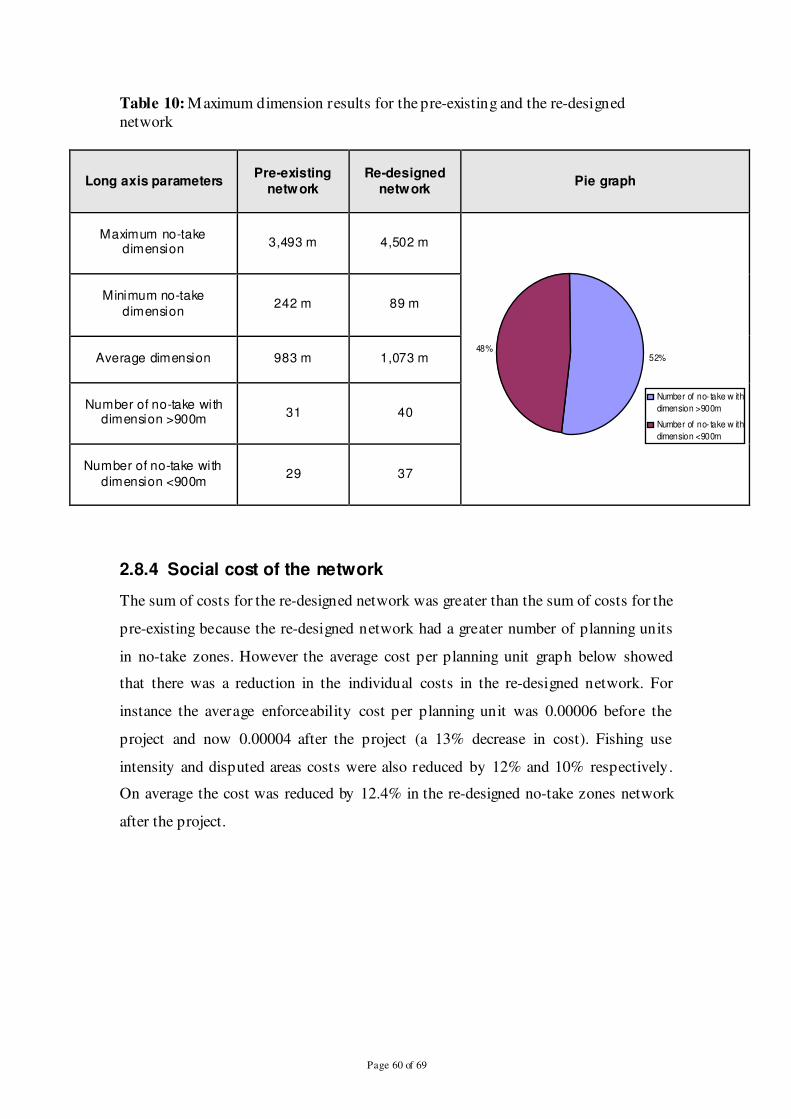
Table 10 showed that the maximum dimension of a no-take zone in the community re-

designed network was over 4,500 meters and the minimum dimension was 89 meters.

The average dimension across the network was over 1,000 meters which was also

higher than the travel distance of Lethrinidae fish species. The number of no-take

zones with dimensions greater than 900 meters was 40 out of 77 (52%) of the total no-

take zones.

of 69

Table 10: Maximum dimension results for the pre-existing and the re-designed network

Long axis parameters

Pre-existing

network

Re-designed

network

Pie graph

Maximum no-take dimension

3,493 m 4,502 m

52%48%


dimension >900m


dimension <900m

Minimum no-take

dimension

242 m 89 m

Average dimension

983 m 1,073 m

Number of no-take with dimension >900m

31 40

Number of no-take with

dimension <900m

29 37

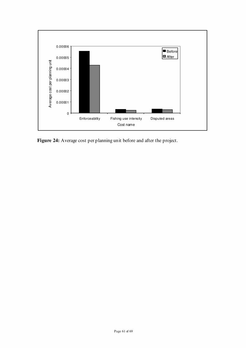
2.8.4 Social cost of the network

The sum of costs for the re-designed network was greater than the sum of costs for the

pre-existing because the re-designed network had a greater number of planning units

in no-take zones. However the average cost per planning unit graph below showed

that there was a reduction in the individual costs in the re-designed network. For

instance the average enforceability cost per planning unit was 0.00006 before the

project and now 0.00004 after the project (a 13% decrease in cost). Fishing use

intensity and disputed areas costs were also reduced by 12% and 10% respectively.

On average the cost was reduced by 12.4% in the re-designed no-take zones network

after the project.

of 69

0

0.00001

0.00002

0.00003

0.00004

0.00005

0.00006

Enforceability Fishing use intens ity Disputed areas

Cost name

Av

era

ge

cos

t pe

r p

lan

nin

g u

nit

Before

After

Figure 24: Average cost per planning unit before and after the project.

of 69

3 Discussion

3.1 Summarizing the effects of redesigning the no-take network

The following bullet points summarize parameter by parameter the effects of

redesigning the no-take zone network. Most show that the redesigned network is

likely to perform better ecologically than the existing.

• The number of no-take zones increased from 60 to 77 (increase by 17 no-take

zones)

• The area protected increased from 29 sq km to 50 sq km (increase of 21 sq.

km)

• The overall percentage of shallow areas protected rose from 12% to 19%

Protection of Geomorphological zone

Across all zones the average number of no-take zones each zone appears in has gone

from 19 to 26.

• There has been a 12% increase in protection of back reef zone across all no-

take zones.

• There has been a 21% increase in protection of channel zone across all no-take

zones.

• There has been an 11% increase in protection of fore reef zone across all no-

take zones.

• There has been a 7% increase in protection of intertidal zone across all no-take

zones.

• There has been a 3% increase in protection of lagoon zone across all no-take

zones.

• There has been an 11% increase in protection of reef crest zone across all no-

take zones.

• There has been an 8% increase in protection of reef flat zone across all no-take

zones.

of 69

Protection of habitat coverage

• There has been a 7% increase in protection of continuous coral habitat across

all no-take zones.

• There has been an 8% increase in protection of patchy coral habitat across all

no-take zones.

• There has been a 9% increase in protection of sparse coral habitat across all

no-take zones.

• There has been a 7% increase in protection of dense seagrass habitat across all

no-take zones.

• There has been a 19% increase in protection of sparse seagrass habitat across

all no-take zones.

• There has been a 13% increase in protection of patchy coralline habitat across

all no-take zones.

• There has been a 7% increase in protection of patchy vegetation habitat across

all no-take zones.

Protection of Significant sites

• The area of spawning aggregations protected increased from 41% to 80%

• The area of turtle nesting sites protected increased from 24% to 61%

• The area of cultural sites protected increased from 7% to 21%

Diversity of habitats

The average number of distinct habitats in each no-take zones did not

increase/decrease before and after the project. The average number of distinct habitat

was 4 across all no-take zones.

Replication of habitats

Across all habitats the average number of no-take zones each habitat appears in has

gone from 29 to 38.

• The number of no-take zones continuous coral appears in has gone from 36 to

48

of 69

• The number of no-take zones patchy coral appears in has gone from 46 to 61

• The number of no-take zones sparse coral appears in has gone from 34 to 45

• The number of no-take zones dense seagrass appears in has gone from 32 to

47

• The number of no-take zones sparse seagrass appears in has gone from 25 to

28

• The number of no-take zones patchy coralline appears in has gone from 16 to

21

• The number of no-take zones patchy vegetation appears in has gone from 11 to

15

Larval settlement

• There was an increase in total hard substrate features from 35% to 42% in the

re-designed network (an increase of 7%)

Spacing

• Maximum spacing distance between two no-take zones was 10,456 (pre-

existing) and 10,543 in the re-designed network (increased by 87 m).

• Minimum spacing distance between no-take zones was 329 in the pre-existing

and 136 in the re-designed network (decreased by 193 m).

• Average distance between no-take zones decreased from 3,131m to 2,602 in

the re-designed network.

Maximizing the contribution of individual no-take areas to the network

• The maximum dimension of the longest axis of no-take zones was 3,493

meters in the pre-existing and is now 4,502 meters in the re-deigned network

(an increase of 1,009 meters).

• The minimum dimension of the longer axis of no-take zones was 242 meters

in the pre-existing and is now 89 meters in the re-deigned network (a decrease

of 153 meters).

• The average dimension of the longer axis of no-take zones was 983 meters in

the pre-existing and now 1073 meters after the re-deigned network (an

increase of 90 meters).

of 69

• Number of no-take zones with dimension greater than 900 meters was 31 in

the pre-existing network and now 40 no-take zones in the re-designed

network.

Cost

• On average the cost was reduced by 12.4% in the re-designed no-take zones

network after the project.

of 69

3.2 Assessing the cost of the design approach It is clear from the above summary of changes that there are likely ecological benefits

that will result from the redesigning process. However, it is prudent to examine the

financial costs associated with this process.

The total project implementation budget for this project was US$97,000

(approximately Fijian $170,000) The main costs included the acquisition of high

resolution imagery (∼US$26,000) and field work costs to collect both social use

information and data used to subsequently derive habitat maps (∼US$ 22,000).

Unpublished work done by the University of the South Pacific has estimated the cost

of all pre-existing marine management work done in Kadavu including establishing

the Kadavu Yaubula Management Support Team at Fijian $140,000.

In the coarsest sense, it is therefore possible to estimate the cost of establishing no-

take zones per unit area. Performing these calculations, it is estimated to have cost

Fijian $4,800 per km2 to establish and maintain the existing no-take zones over an

average of 4.6 years.

With an increase in protection of 21km2 during the redesign process, the average cost

per unit area of the redesign process was approximately Fijian $8,100.

Interestingly, with most the expenditure being made on satellite imagery, it was felt

by the project team that the main value of the project was in providing opportunities

for communities to sit, assess their existing protection efforts and plan new and

expanded no-take zones. Arguably with the cost associated with a scientific redesign,

this could have been achieved at a far lower cost per unit area protected.

of 69

3.3 Lessons learned and recommendations

1. The inclusion of social cost layers is essential in the development of a

no-take redesign- factors such as enforceability and local conflict are

as important as lost opportunity cost of, for example, fishing.

2. The reserve design process used in this project was successful in

promoting the inclusion of additional areas in protection; and

contributed to better reflection of networking principles; and managed

to achieve so at a lower lost opportunity cost (fishing, enforcement

etc).

3. Community participation is essential- in many ways, Fiji lends itself to

such a project where customary marine tenure dictates the implicit

involvement of communities.

4. In many instances the stakeholders involved in the design and re-

design of no-take zones in Fiji are few; there are not large commercial

fishing fleets in inshore areas and tourism operations are, aside from in

a few areas, sparsely distributed. Therefore some of the complexities of

redesigning protected area networks found elsewhere are not

applicable in Fiji.

5. The reserve design process used has proven expensive per unit area

protected- arguably the value was in engaging with communities and

similar results could have been achieved at a lower cost per unit area.

6. It is worth examining more cost-effective means to derive the input

data used in the reserve design process. For example, it maybe possible

to use community drawn maps instead of those derived from satellite

imagery; or use a lower descriptive resolution based on

geomorphological ecological proxies.

of 69

4 References

• Hastings, A. and Botsford, L. W. (2003). Comparing designs of marine

reserves for fisheries and for biodiversity Ecological Applications, 13(1)

Supplement, 2003, pp. S65–S70q 2003 by the Ecological Society of America

• Blaschke, T. (2010). "Object based image analysis for remote sensing",

Journal of Photogrammetry and Remote Sensing

• Center for Spatial Environmental Research (CSER). Data accessed online at:

(http://www.gpem.uq.edu.au/cser)

• Roelfsema, C., Phinn, S., Jupiter, S., Comley, J., Beger M. and Paterson, E.

(2010). The application of object based analysis of high spatial resolution

imagery for mapping large coral reef systems in the west pacific at

geomorphic and benthic community spatial scales. Center for Remote Sensing

and Spatial Information Science School of Geography, Planning and

Environmental Management, University of Queensland, Australia.

• Roberts, C. M., Branch, G., Bustamante, R. H., Castilla, J. C., Dugan, J.,

Halpern, B. S., Lafferty, K. D., Leslie, H., Lubchenco, J., McArdle, D.,

Ruckelshaus, M. and Warner, R. R. (2003). “Application of ecological

criteria in selecting marine reserves and developing reserve networks”

Ecological Applications. 13 (1), pp. 215-228. Data accessed online at:

http://repositories.cdlib.org/postprints/970

• Congalton, R. G. and Green K. (1999). Assessing the accuracy of remotely

sensed data: principles and practices. Boca Rotan FL, Lewis Publishers: 137.

• Fiji Island Bureau of Statistics, 2008 Fiji Facts and Figures. Data accessed

online at: http://www.statsfiji.gov.fj/FFF08.pdf

• Island Directory (1998). Data accessed online at:

http://islands.unep.ch/CLQ.htm

• IUCN World Commission on Protected Areas (IUCN-WCPA) (2008).

Establishing Marine Protected Area Networks—Making It Happen.

Washington, D.C.: IUCN-WCPA, National Oceanic and Atmospheric

Administration and The Nature Conservancy. 118 p.

• Leslie, H. M. (2005). A Synthesis of Marine Conservation Planning

Approaches. Conservation Biology 19(6): 13.

of 69

• Watts M. E., Stewart R. R., Segan, D., Kircher, L. and Possingham H. P.

(2010). Using the Zonae Cogito Decision Support System. Data accessed

online at: http://www.uq.edu.au/marxan/zonae-cogito-software.

• National Research Council (NRC) (2000). Marine Protected Areas: tools for

sustaining ocean ecosystems. Washington, D.C., USA, National Academy

Press.

• Nunn P. D. (1999). Penultimate Interglacial emerged reef around Kadavu

Island, Southwest Pacific: implications for late Quaternary island-arc tectonics

and sea-level history. Data accessed online at:

http://royalsociety.org.nz/Site/publish/Journals/nzjgg/1999/15.aspx

• Phinn, S.R., Roelfsema, C.M. and Mumby, P.J. (in press). "Multi-scale image

segmentation for mapping coral reef geomorphic and benthic community

zone", Int. J. Remote Sens.

• PISCO. 2007. The Science of Marine Reserves (2nd Edition, United States

Version), Partnership for Interdisciplinary Studies of Coastal Oceans, 22.

• Roberts C. M., Halpern, B., Palumbi, S. R. and Warner, R. R. (2001).

Designing Marine Reserve Networks: Why Small, Isolated Protected Areas

Are Not Enough. Conservation 2(3): 10-17.

• Airame, S., Dugan, J E., Lafferty, K D., Leslie, H., McArdle, D A. and

Warner, R. R. (2003). “Applying ecological criteria to marine reserve design:

A case study from the California Channel Islands”. Ecological Applications.

13 (1), pp. 170-184. Data accessed online at:

http://repositories.cdlib.org/postprints/971

• The Locally Managed Marine Areas Network. Data accessed online at:

http://www.lmmanetwork.org/

• Watts, M. E., Klein, C. K., Stewart, R., Ball, I. R. and Possingham. H. P.

(2008). Marxan with Zones (V1.0.1): Conservation Zoning using Spatially

Explicit Annealing, a Manual.

technical report: development of a network of...

Documents