ESD-TR42-IU

: q "

C1 Technical Report 620

W. Rotman

EHF Dielectric Lens Antenna for

Satellite Communication Systems

3 January 1983

Preper-d for the Department of the Air Force

under iectronic Systems Division Contract F1gB28-0-C 0( by

Lincoln LaboratoryMASSACHUSETTS INSTITUTE OF TECHNOLOGY

LEXINGTON, MASsuCnusETIS

Approved for public release; distribution unlimited.

EL

83 03 30 '06.

-. . . . . . . -' ,

The work reported in this document was perfonned at Lincoln Laboratory, a centerfor research operated by Massachusetts Institute of Technology, with the support ofthe Department of the Air Force under Contract F19628.80-C.0002.

This report may be reproduced to satisfy needs of U.S. Government agencies.

The views and conclusionscontained in thisdocument are those of thecontractorandshould not be interpreted as necessarily representing the official policies, eitherexpressed or implied, of the United States Government.

The Public Affairs Office has reviewed this report, and it isreleasable to the National Technical Information Service,.where it will be available to the general public, includingforeign nationals.

This technical report has been reviewed and is approved for publication.

FOR THE COMMANDER

Thomas J. Alpert, Major, USAFChief, ESD Lincoln Laboratory Project Office

Non-Lincoln Recipients

PLEASE DO NOT RETURN

Permission is given to destroy this documentwhen it is no longer needed.

I--

MASSACHUSETTS INSTITUTE OF TECHNOLOGY

LINCOLN LABORATORY

EHF DIELECTRIC LENS ANTENNA FORSATELLITE COMMUNICATION SYSTEMS

W. ROTMAN

Grou I

TECHNICAL REPORT 620

3 JANUARY 1993

Approved for public release; distribution unlimited.

LEXINGTON MASSACHUSETTS

~ABSTRACT

Dielectric lens antennas are applicable to the design of ml iple-beas

antenna (IMBA) systems on E}, communication e llite. Advantaes include

excellent wide angle scanning properties and elimination of feed blockage.

This report describes an experimental 90 dis. zoned dielactric lens,

operating at 44 GHrwhich was fabricated and tested in order t estimate the

performance of a dielectric lens MBA. Measurements showed that the lens

generated a beam with a half-power beamwidth (HPBW) of 0.7 which could be

steered over a total scan angle of 18 (corresponding to the earth's field-of-

view from a geosynchronous satellite) with a scanning loss of less than I dB

and a gain in excess of 47 dBi weas ed at the sub-satellite point over a 5%

bandwidth. A theoretical analysis /of the radiation characteristics of the

lens antenna, using ray tracing and geometric optics techniques, gaveI/

excellent agreement with the measuements. Simplified design equations were

developed to facilitate evaluation and development of lens antenna systems of

this type.

Acession For/1 ~NTIS 0OA&I

DTI!C TAB fJusti leer i-

i] ii

Dst-ribution/Avalabtlity Cwldes

... rDist spoe iea l

CONTENTS

Abstract lit

List of Illustrations Vi

List of Tables viii

I. Introduction 1

1I. Selection of Lens Parameters 7

III. Thin Lens Theory 12

IV. Phase Errors in Zoned Lenses 22

V. Effects of Beam Scanning on Radiation Patterns 30

VI. Effects of Beam Scanning on Antenna Gain 49

VII. Comparison of Measured Versus Theoretical Antenna Gain 54

VIII. Conclusions 58

Appendix A: Design Parameters for 23.5" Da. Zoned Lens 61

Appendix B: Ray Trace Equations for Zoned Lenses (Method A) 65

Appendix C: Calculation of Gain and Radiation Patterns of ZonedLens (Method A) 73

References 78

Acknowledgments 80

V

I. _- J

ILLUSTRATIONS

Figure No.

1. Lens antenna system for satellite communications fromgeosynchronous orbit. 2

2. Loss of directive gain with scan angle for coma-corrected lens. 4

3. Zoned dielectric lens with feed. 9

4. ElF aplanatic dielectric lens with multiple feeds. 10

5. Design of zoned dielectric lens. 11

6. Ray-trace analysis of zoned lens (Method A). 13

7. Representative focal arcs for thin dielectric lensse. 18

8. Frequency-dependent component, 8f, of lens path length error. 23

9. Path length errors in zoned lens. 26

(a) 43.5 GHz; a - 0* 26(b) 43.5 Gs; a - 8.6; - 00 26(c) 43.5 GB:; a - 8.6; * = 45o 26(d) 43.5 G1L; a - 8.6*; - 90 26

(e) 44.5 GHz; a - 0* 27(f) 44.5 GHz; a - 8.6; - 0 27(g) 44.5 Giz; a - 8.6*; - 45 27(h) 44.5 GRz; a - 8.60; - 90 27

(1) 45.5 Gl:z; a - 0* 28(J) 45.5 Giz; a - 8.6; - 00 28(k) 45.5 Gbz; a - 8.60; 450 28(1) 45.5 Giz; a - 8.60; = 90 28

" 10. Stationary optical path analysis of zoned lens (Method B). 31

11. Coordinate system for far-field calculations. 32

12. Theoretical radiation patterns of zoned lens: (a) 43.5 GHz(b) 44.5 Gbs (c) 45.5 Gz [Curve A: a = 0; Curve B: a - 8.6%

- 900; Curve C: a = 8.60, ' " 001 34

vi

ILLUSTRATIONS (cont'd)

13. Feed horn dimensions 37(a) short horn (r - 0.403 in)(b) long horn (r = 0.568 in)

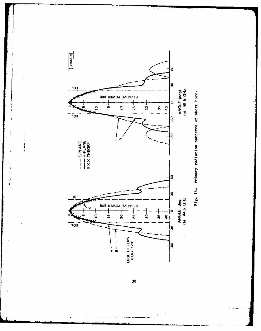
14. Primary radiation patterns of short horn: (a) 44.5 ftz(b) 45.5 0HRz. 38

15. On-axis radiation patterns of zoned lens with short horn(44.5 G0z). 40

16. On-axis radiation patterns of zoned lens with long horn

(44.5 CHz). 41

17. Off-axis radiation patterns of zoned lens (44.5 GHz). 43

18. Measured radiation patterns of zoned lens (45.5 CHz). 44

19. Measured radiation patterns in scan plane as a function offeed horn tilt angle, $ (44.5 GHz; a - 8.6"; = 90). 46

20. Measured radiation patterns in orthogonal plane as a functionof feed horn tilt angle, 0 (44.5 GHz; a - 8.6*; # - 0). 47

21. Scanning loss L(a) versus path length error in zoned lens. 53

22. Scanning loss L(a) of lens antenna with feed position 1. 57

A-1. Zoned dielectric lens of dimensions. 62

B-I. Ray path In lens antenna (PIP 2P3Q) . 66

vii

TABLES

Table No.

I. Scanning aberrations for experimental lens paraietere 21

11. on-axis gain of zoned lens 55

viii

I. INTRODUCTION

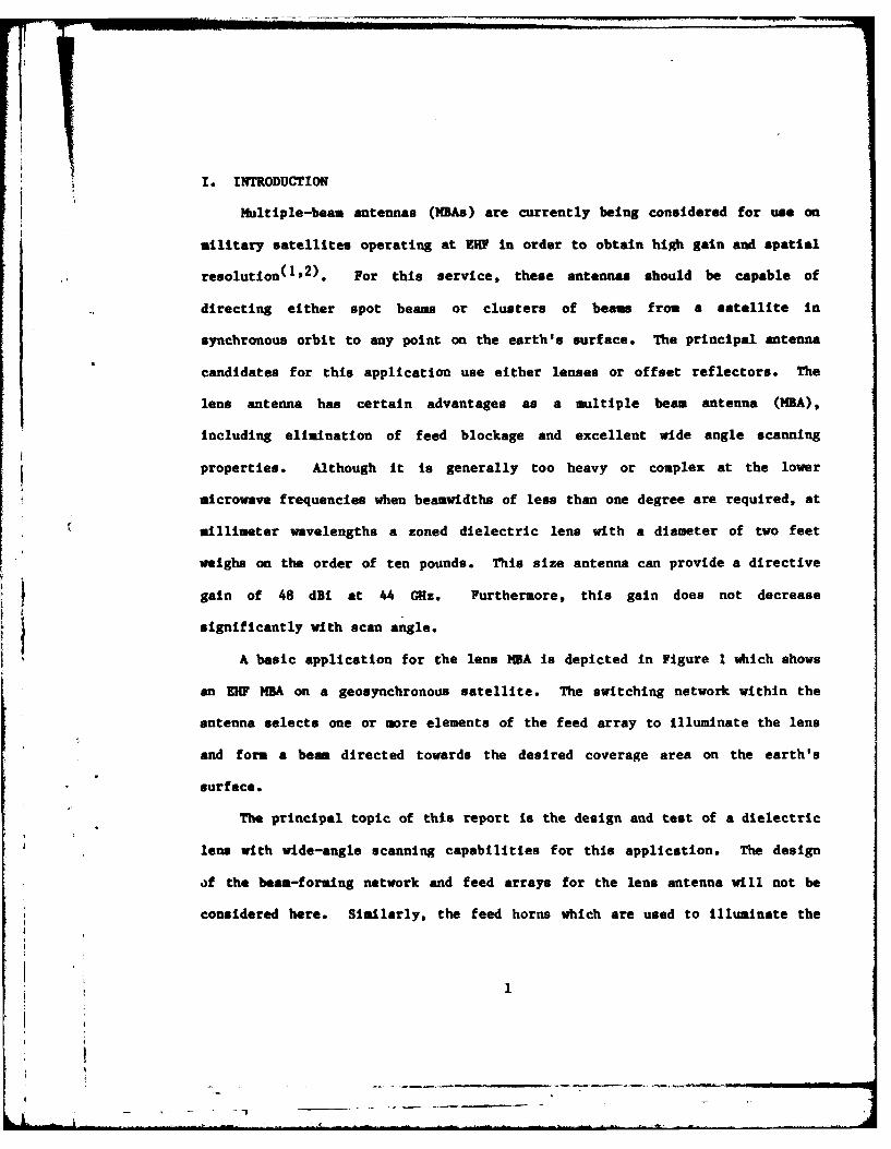
Multiple-beam antennas (MBAs) are currently being considered for use on

military satellites operating at EU! in order to obtain high gain and spatial

resolution (1 ,2 ). For this service, these antennas should be capable of

directing either spot beams or clusters of beaus from a satellite in

synchronous orbit to any point on the earth's surface. The principal antenna

candidates for this application use either lenses or offset reflectors. The

lens antenna has certain advantages as a multiple bean antenna (MBA),

including elimination of feed blockage and excellent wide angle scanning

properties. Although it is generally too heavy or complex at the lower

microwave frequencies when beamwidths of less than one degree are required, at

millimeter wavelengths a zoned dielectric lens with a diameter of two feet

weighs on the order of ten pounds. This size antenna can provide a directive

gain of 48 dBl at 44 GHz. Furthermore, this gain does not decrease

significantly with scan angle.

A basic application for the lens MBA is depicted in Figure I which shows

an EHF NBA on a geosynchronous satellite. The switching network within the

antenna selects one or more elements of the feed array to illuminate the lens

and form a beam directed towards the desired coverage area on the earth's

surface.

The principal topic of this report is the design and test of a dielectric

lens with wide-angle scanning capabilities for this application. The design

of the beaa-forang network and feed arrays for the lens antenna will not be

considered here. Similarly, the feed horns which are used to illuminate the

41* I--- - - - - - - . -

LUU

LUU

4U W

z U

CI

>-E0 J5

L'-.

4 U

-- J

ti

LUU

u-zm

2o

lens are analyzed only to the extent to which this serves the evaluation of

the lens performance.

A major problem in the design of this multiple-bean lens antenna is the

requirement to direct a beam with a fractional degree beamwidth from a

satellite over the entire earth's field-of-view 7) of 18* total scan angle

without incurring excessive reduction of gain. 's decrease in directivity

with scan angle will be shown to be related to tt ff-axis aberrations of the

lens, which are minimal for an idealized spherich ,a of zero thickness with

its focal point at its center of curvature. Although this ideal cannot be

achieved in practice, it can be approximated by zoning, or stepping the

thickness of the lens. This zoning also has the beneficial effect of reducing

the weight of the lens; however, these benefits are partially offset by an

increase in frequency sensitivity. Partial zoning offers a reasonable

compromise for many applications between off-axis performance, bandwidth, and

weight considerations.

The decrease in gain of the lens, caused by variations in frequency from

the design value and by scanning along an optimum focal path, can be estimated

from the simple thin lens equations, presented in Section III, which are

appropriate for zoned lenses with spherical outer faces. Figure 2 shows this

loss L(c) as a function of scan angle a for 90), (diameter) lenses with seven

zones and with focal length to diameter (F/D) ratios of either 1.0 (dashed

lines) or 1.5 (solid lines). The two curves for cach F/D ratio represent the

losses at the center, or design frequency (f - fo; Af - 0), and at the band

edges (Af/fo - 2.5%), respectively. (These curves are obtained as special

3

. i -_ __ - ----- __ _

w-

> 0w o,

0 40

sU

C,w

0

C%4 N

UL C4

0o 0

(ap) Ml- sso 0

cases of the general scanning loss curves of Fig. 21). These estimates

predict that for our experimental lens (90A, F/D - 1.5, 7 zones), the scanning

losses over the earth's FOV (* 90) should be less than 0.2 dB at the design

frequency and 0.5 dB at the band edges. The excellent scanning

characteristics of the lens, which these values predict, have been verified

generally by the more accurate ray trace analyses and antenna measurements

which are described in this report.

A qualitative comparison of the scanning performance of lens anttnnas with

various types of reflectors is instructive in evaluating potential system

applications. Prior studies( 3'4 ) have shown that the loss in gain with scan

angle of symmetrical, coma-corrected reflectors and of thin lenses with the

same F/D ratios are identical. However, since the feed in a reflector usually

is offset from its axis of symmetry in order to prevent obscuration of the

aperture, scanning must be essentially one-sided in the offset plane.

Furthermore, the simple parabolic reflector is not coma-corrected. (Although

this could be accomplished by stepping its surface, the resultant reflector

would then be frequency-sensitive, similar to the lens.) The zoned dielectric

lens would, therefore, be expected to have superior scan characteristics over

any prime-focus symmetrical reflector system of the same F/D ratio since

offsetting is not necessary and the lens is essentially coma-corrected.

Some improvement may be achieved in the beam steering characteristics for

an asymmetrical offset-fed reflector so that it has same phase errors (5 )

(third order) as a symmetrical reflector for equal displacement of the feed

laterally from the prime focus. Although this change avoids the offsetting

5

loss which is inherent in the symmetrical systems, the reflector scan still

sust be slngle-sided and, therefore, inferior to lens scanning. The situation

is not so clear for offset Cassegrain reflector systems, however. In this

case, the scanning performance can be evaluated from the equivalent parabola

concept in which the equivalent focal length is increased over the physical

focal length by the magnification factor of the antenna system. The

equivalent F/D ratio may, therefore, be several times that of a lens with the

same physical dimensions with a corresponding improvement in scan

capability. Since this advantage will be partially nullified by the one-sided

scan requirement of the offset reflector, the lens and Cassegrain reflector

are likely to have comparable beam steering properties although an exact

evaluation can probably only be made on a case-by-case basis.

6

II. SELECTION OF LENS PARAMETERS

Although the weight of the lens is a major factor affecting its design

for satellite applications, light weight artificial dielectric and constrained

lenses were excluded from consideration because of their complexity and

difficulty of fabrication at EHF frequencies. An unzoned dielectric lens of

90A diameter (the design dimension) is relatively heavy at 0 band (44 GRz),

ranging up to almost 70 pounds for a solid lens (polyethylene) with an F/I of

1.0. This weight can be drastically reduced through zoning and increasing the

F/D ratio. (This also has the commensurate effect of reducing the scanning

losses, as previously mentioned.)

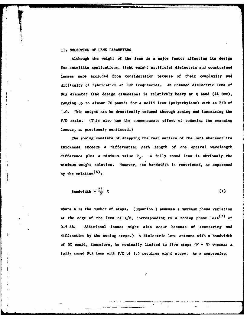
The zoning consists of stepping the rear surface of the lens whenever its

thickness exceeds a differential path length of one optical wavelength

difference plus a minimum value To . A fully zoned lens is obviously the

minimum weight solution. However, its bandwidth is restricted, as expressed

by the relation(6):

Bandwidth -- 2 (1)N

where N is the number of steps. (Equation 1 assumes a maximum phase variation

at the edge of the lens of X/8, corresponding to a zoning phase loss ( 7 ) of

0.5 dB. Additional losses might also occur because of scattering and

diffraction by the zoning steps.) A dielectric lens antenna with a bandwidth

of 5% would, therefore, be nominally limited to five steps (N - 5) whereas a

fully zoned 90A lens with F/D of 1.5 requires eight steps. As a compromise,

7

six steps were used in the experimental model, accepting the increased scan

los at the frequency band limits.

The design of the lens (Figures 3 and 4) follows exactly the detailed

procedure given In reference 8, except that the lens is partially, rather than

completely, zoned. Detailed dimensions of this lens, including its scaled

cross-section, are presented In Appendix A. Its outer (front) surface is

spherical, with the center of curvature at the focal point. The inner (rear)

surface is determined by equating the optical path length of a ray from the

focal point through the lens to that of the central ray (Figure 5) (stepping

the lens thickness whenever It exceeds a differential wavelength). For

machining, the central and first outer zones for the inner surface of the lens

are represented by a fourth degree polynomial; the outer five zones are

approximated by straight line segments, determined by the points of

discontinuity and corners on the contour. These approximations specify the

inner contour of the lens to within two mils of the theoretical surface. The

lens was machined on a numerically controlled lathe In accordance with these

specifications.

8

r

C 'V6,6,

'4-

'5'-4

6i

I.''5

( U6,

'-4a.,

'-4'V

'VS

CC.'

9

-i -------- - --- _______ --- -

-

LLI

w 00

I 41(~ + 0 I

a cc00

I 1 'tiI:.jLL. U.

101

Z LA

-j-

LUU

LAA

C-)

zN

-WJ

* :ii.

* ~64

Ill. THIN LENS THEORY

Although the experimental lens has been designed to be without aberration

for an on-axis feed at the design frequency, phase errors will occur in the

wavefront of the radiated beam as it is scanned and as frequency changes.

Scanning Implies a linear change in the wave front as the primary feed of the

lens is displaced along a focal arc. The radiated beam is then pointed

approximately in the direction given by the line joining the feed to the apex

of the lens. The aberrations in the phase of the avefront cause a decrease

in gain, increase in sidelobe level and broadening of the main beam of the

radiation pattern. The wide angle scanning capabilities of the experimental

lens may, therefore, be evaluated through the near-field determination of both

phase and amplitude in the lens aperture.

A complete analysis of the lens requires consideration of the aberrations

due to stepping and edge diffraction, as well as those due to the asymmetric

amplitude illumination which results from scanning. This detailed evaluation

is beyond the scope of the present paper. Our analysis will be restricted to

geometrical optics effects for which ray-tracing is applicable. In the first

approach (Method A) a ray is traced from the feed through the lens to a plane

parallel to the radiated wavefront (Figure 6). The aberrations are given by

the difference between the electrical path length of this ray and the

principal ray which goes through the apex of the lens. [A second approach

(Method B), which traces rays back from the front surface of the lens to the

feed position, will be presented later in this report.]

12

zz

_Its

L"4wC

I 0"ACL~

LU CL

tiS

L"4

w5.

LL 0

13

As a first approximation, the lens is assumed to be of zero thickness

(ideally thin) so that the analysis developed in Reference 6 applies. In that

paper, the wavefront aberrations, 6 n, are expressed as a power series of the x

and y coordinates, measured in a plane normal to the lens axis. Only the

second and third terms of the power series are considered, giving the

spherical aberration, 62, and coma, 63. (The first order term is a linear

bean shift. Higher order terms are negligible at small scan angles.)

Spherical aberration, 62, is determined by the scanning locus (focal arc)

and is shown( 7 ) to be independent of the shape of the lens. The scanning

locus may always be chosen so that 62 is zero in any specified plane. The

curvature of the scanning locus is greatest if 62 is reduced to zero in the

plane of scan and least if 62 is reduced to zero in the plane orthogonal to

the plane of scan.

Coma, 63, is mainly a function of the inner profile of the lens. A

perfectly thin lens with a front surface radius R equal to its focal length f

obeys the Abbe Sine condition and has minimum coma. For a lens with F/D > 1.0

and a < 30, the effects of coma are negligible in comparison with spherical

aberration (the only remaining significant term) which is given by (Eq. 1 of

Reference 7):

2 2 1 2 f(

14

where (Figure 6)

f - focal length

I - distance from scanning position to apex of lens

a - scan angle

(The x and y coordinates of Eq. 2 are measured in an aperture plane which

passes through apex of the lens and is normal to its axis of symetry

(z axis). The feed is assumed, without loss of generality, to move only in

the y-z plane during scanning.)

We will now use Eq. 2 to investigate the effect of the scanning locus of

the feed on 62. If the scanning locus is defined by

2I - f cos a C0)

then 62 - 0 in the plane of scan (y-z plane; x - 0). If it is defined by

I- f (4)

then 62 - 0 in the ortlogonal plane (x-z plane; y - 0.) A compromise locus

for the thin lens, which balances the aberrations in the y-z and x-z planes is

then given by the average value of L in Eqs. 3 and 4:

1 2t f(L + cos a) • (5)

15

(Equation 5 defines that scanning locus on the focal surface for which most of

the experimental lens data were obtained.)

Equation 2 shows that 82 lacks circular symmetry since the presence of

astigmatism is evidenced by the inequality of the terms Involving x2 and y2.

This fact is emphasized by writing Equation 2 for the compromise focal arc in

terms of cylindrical coordinates, r and *, in the x-y plane where

y - r sin (6)x w r cos

Substituting Eq. 6 into Eq. 2:

2 2f Itcs 2f (-Z

L-1 [f I in a - 1 + sn atcos 2

where:

88 r 2r [ I stn'a) _ ](8)

2[1a r f s in 2 2 cos 2# (9

a aR

16

LI --

I

The term s. has circular symmetry and represents defocussing, or first order

spherical aberration, while Sa is asymmetrical and represents astigmatism.

(These definitions are in accordance with the classification of the primary

(Seidel) aberrations (9 1 , but are at variance with those used in Reference 7.)

The maximum aberrations for a given scan angle, a, are obtained at the

edge of the lens for which r equals the lens radius a. Then, Eqs. 8 and 9

become

(6lmx - [f 1 2

a2 + Lf[(sin 2 a cos 2#) 1 (11)(6a)max - + a

a - D/2 - lens radius.

We will now consider the phase aberrations (Eqs. 8 and 9) associated with

four specific scanning loci (Figure 7).

Case I (Circular locus with center at apex of lens):

f (12)

1 22- -41-r /f ) (sin a) (13)

a +(r 2 /f) (sin 2 a cos 2.) (14)

17

wL

Izi QZ ~LL I~cc

0'U- D

010

Co 00,I

181.

The phase aberrations are divided equally, In this case, between

astigmatism and first order spherical aberration.

Case 2 (Flat focal plane):

I.f/cosa (15)

2 12

6~ = -~{/f)[1cs -(c083o c) (6

6 + -L(r2/)(o ai-cs )(cos 2*)] (17)

Case 3 (Eq. 3):

-08 ao~ (18)

6S + 1j(1-)[tan 2 a] (19)

6 +4 -(r /f)[tan ai cos 2.] (20)

19

Case 4 (Compromise focal arc):

1 2

_I(cos a + 1)f (21)

6 0 (22)

6 1 (r/)[ sin2 ][cos 2.] (23)I + cos a

The primary spherical abberation term 6. has therefore vanished in this

latter case, leaving only the astigmatism term 6a Note that, in all four

cases, the astigmatisu term varies only slightly while primary spherical

aberration depends strongly on the curvature of the focal arc. This can be

seen by calculating the maximum spherical and astigmatic aberrations (6

and (Sa~max from Eqs. 10 and II for the above cases, using the experimental

lens parameters (Table I: a - 9'; F/D = 1.5; D = 90X).

20

TABLE I

SCANNING ABERRATIONS FOR EXPERIMENTAL LENS PARAMETERS

Case 1/f 68m/x(6,a).axk coo 2

1 1.0000 -0.092 +0.092

2 1.0124 -0.183 +0.091

3 0.9755 +0.094 +0.094

4 0.9877 u +0.093

21

IV. PHASE EKKES IN ZONED LENSES

The zoned lens can be considered to be a reasonable approximation to the

thin lens with respect to phase aberrations over its aperture. The major

difference is that a frequency-dependent phase error term 6f is introduced due

to the zoning. This effect will now be evaluated by comparing ray path

calculations in the zonea lens with the approximate thin lens results derived

in the last section.

The frequency sensitivity of the lens can be derived approximately for

the on-axis case by noting that path length discontinuities of one wavelength

occur at each step. Since the phase is modulus 2w, this does not result in

any phase error at the design wavelength Xo for an on-axis feed. However, at

any other wavelength X, the path length error AXT, relative to the central

ray, is given by:

AtAAl/ )n (24)

where n is the step number (starting from the center of the lens). Figure 8

shows this path length error for the experimental lens at the band extremities

(43.5 and 45.5 GHz), both as a discontinuous curve with phase jumps at the

steps and as a continuous approximation. (The position of the steps are

obtained from Appendix A). We will show that the total phase (path length)

errors in the zoned lens can be obtained approximately by adding this

frequency-dependent term 6f to the thin lens values, 6s and 6a-

22

L

020

0.15

STEPPED PATH ERRORS

010 CONTINUOUS APPROXIMATION

45.5 GHz

_1

0.05

z -Ilc-,_ 44.5 GHz I0

U-I

-0.05 -L

aI ~43.5 GHz

010

-015

LENS EDGE

-0 20 I I I I0 2 4 6 8 10 12

LENS RADIUS (in.)

Fig. 8. Frequency-dependent component, 6f, of lens path length error.

23

The equations used in Method A to trace rays from an arbitrary feed

position through the lens to the aperture plane and to determine the resultant

path length differences are presented in Appendix B. In this approach

(Figure 6), the feed Is assumed to lie in the y-z plane at a position P1 (O,

Yl. zj). (The (x, y, z) coordinate systems have their origins at the apex of

the lens.J The ray under consideration intersects the rear surface of the

lens at a specified point P2(x2 , Y2, z2) or, in cylindrical coordinates, P2(r,

*, z2 ). Snell's law then determines the refraction of the ray at this surface

and its suosequent intersection with the front lens surface (a sphere with

defining equation [x2 + y2 + (I + Z)21 _ R2 ) at the point P3(x3, Y3 1 33).

From here, the ray is assumed to be normally incident upon the wavefront

reference plane which is orthogonal to the beam direction. (This last step is

a simplifying assumption which is valid, in accordance with Fermat's

principle, for small path length errors.) The total path length LT is

calculated from the three ray components:

T t 2 + t3 (25)

where

- P = distance from feed to rear lens surface,

t2 = P2P3 = distance from rear to front lens surfaces,

24

13- - distance from front lens surface to output reference plane,t33

p = index of refraction of lens dielectric,

The path length difference AT iS then obtained as the difference between

LT for the general ray and that for the central ray, which passes through the

apex of the lens.

These normalized path length differences (ALT/A) are plotted in Figure 9

as a function of radial distance from the apex of the lens for a feed which is

located on the compromise scanning locus [t - 1/2(cos2a + l)f] for both on-

axis (a-00) and off-axis (a - 8.6*) positions. The solid curves are the

computer outputs from the ray tracing program while the dashed lines are the

thin lens approximations, including the frequency-dependent term 6f, from

Rqs. 23 and 24 (62 - 6a + 6f; 6s - 0). The calculations are shown for three

different cuts through the aperture plane of the lens (* - 00, 45, 90*) and

for three frequencies (43.5, 44.5 and 45.5 GRz). In the thin lens

approximation the path length error is zero over the aperture (Figure 9e) for

the on-axis (a - 0") feed position at the design frequency (44.5 Clz). At all

frequencies the astigmatism term 6a disappears for both the on-axis case

(Figures 9a, e, i) and the * = 450 cuts (Figures 8c, g, k), leaving only the

frequency-dependent term 6f. Likewise, 6f is zero at the design frequency for

any feed position, leaving only astigmatism (Figures 9e, f, g, h). Both the

frequency and astigmatism terms are present at frequencies other than the

design frequency for the off-axis feed in the principal planes (0 * 0 and

900; Figures 9b, d, J, 1). It can be seen that the thin lens approximations

25

/0

ItI

0 0L 0o00 (0 d

1I 9

jo~ jjaHON1HS

32

I o

0 0 cc

It 0

(00 (0

(/9J /IV 440HII H~

a 27

I -0

11 If

00

(y/z jocoo)jiaHO31H

28c

lens approximations follow the trends of the ray trace results in all cases

and could be used to predict the radiation characteristics of the lens design

with reasonable accuracy and a minimum amount of computation.

29

L i - ----

V. EFFECTS OF BEAM SCANNING ON RADIATION PATTERNS

The far-field radiation patterns of the zoned lens were calculated by two

different techniques. In Method A (Fig. 6) the fields are integrated over a

circular aperture in the plane normal to the beam direction. This procedure

makes use of the output of the ray trace program discussed in the previous

section. In the second approach (Method B) the rays are traced backwards from

the spherical front lens surface to the feed (Figure 10; P3 to P2 to PI). The

intensity of illumination over this surface is then evaluated from the power

contained within ray bundles emanating from the feed. Finally, the far-field

radiation patterns are computed by an integration over the lens surface.

Typical radiation pattern and gain computations obtained by both of these

methods are now presented for comparison with experimental results and with

the thin lens approximations.

In Method A the far-field, unnormalized, radiation pattern F(e',.') of a

circular aperture of radius a in a plane is given by(10):

a 2w

F(f',*') -J dr f d$ E(r,#) exp{jkr sine' cos(' - 0)} (26)

0

where k - 2w/A.

Here, E (r,*) is evaluated at the lens aperture coordinates (r, #) while the

far-field amplitude F(8',4') is evaluated at the polar coordinates (e',f')

where e' and *' are measured in a coordinate system oriented relative to the

beam direction (Figure 11). The complex amplitude E(r,*) can be written in

the form:

30

W wcc wZ

-u Zo

00

0

CLi

-- 4

W 0

14

co

w ~ -41

0 0

-Zw

ww 0

1. KN ui31

V, 1 2 3056tNJ

I - PROJECTED

\ AP'*RTURELENS

APERTURE/

/XBIEAMT/ON TO FAR-FIELD

/ 0~- POINT (PO 01)

Fig. 11. Coordinate system for far-field calculations.

32

- (r,*) ej8(r) (27)

where Em(r, ) is the magnitude of the aperture field and the constant B(r,#)

is determined from the path length differences of the rays as

S(r,o) - 2w (AtT)/A (28)

Under tne assumption that tire aperture illumination function is

circularly symmetrical [IE(r,4)l = Em(r)], the directive gain G(a) may be

obtained by an integration over the aperture plane:

E(r, ) r dr d.I

G(a) = [8/ 2 ] (29)

S IE(r,)i 2 r drf0

(Alternatively, the gain may be computed by integrating tae far-field

radiation patterns.) Details of the pattern and gain integration pre-edures

are presented in Appendix C.

Typical radiation patterns, calculated from Equation 26, are shown in

Figure 12 for an assumed aperture distribution of the form

2r. - 1 - r2 ) (3U)

33

I.

0 :1

00

- 64,

C4.

- IL

304

where " is the normalized lens radius . For the feed on-axis (a-O*), the

patterns exhibit the sharp nulls and low sidelobes at the design frequency

(44.5 GHz) which are expected from a uniform phase distribution, while showing

wider main beams, fill-in of the first nulls, and higher sidelobes at the band

edges (43.5 and 45.5 GHz). This pattern degradation is evidence for the

existence of frequency-dependent phase errors. (Compare curves A of

Figs. 12a, b, c with the corresponding phase error curves of Figures 9a, e,

i.) Similarly, the principal plane cuts in the radiation pattern for the off-

axis feed position (a - 8.60; 0 * 0° and *' - 90*; Curves B and C in Fig. 12b)

are essentially identical to each other at the design frequency since the

phase errors due to astigmatism are almost equal in both planes and no other

phase errors are present.

The situation becomes more complicated for the off-axis feed and at the

frequency extremes since both frequency-independent and scan-dependent phase

errors are simultaneously present, and they can tend either to reinforce or

cancel each other. At the lower end of the band (43.5 GHz), the beam is well

focussed in the orthogonal plane ( ' - 0*), where the phase errors tend to

cancel, and defocussed in the scan plane ( ' - 90*), where the errors add.

These effects are reversed at the upper frequency limit (45.5 GHz) where the

beam is well focussed in the scan plane and defocussed in the orthogonal plane

(See Figs. 12a, 12c, 9b, 9d, 9j, and 91.) The reason for this reversal is the

*Equation 30 is the same illumination function which was assumed in

References 3 anA 7 for the evaluation of scanning losses and performance of alens antennas. It is a first-order approximation to the lens illuminationproduced by a feed horn, which would P-'ually vary as a function of feedposition on the scan locus and would prenetally be asymmetrical.

35

change in sign of the frequency-dependent phase error (Eq. 24) between the

lower and upper frequency limits. These comparisons show that the thin lens

equations provide a reasonable and rapid estimate of the radiation

characteristics of the zoned lens, as an alternative to the more accurate but

more complex ray trace calculations.

The radiation patterns of the lens were measured over a 43.5 to 45.5 QI:

frequency range, using two different feed horns. These feeds (Figure 13) are

scaled models of a dual-mode conical horn (shown in Figure 12 of

Reference 11), designed for equal beamwidth In its F and H planes. The

radiation patterns of this type of feed horn are designed to be circularly

symmetrical and essentially identical to the H-Plane pattern of an open-ended

circular waveguide carrying the TE11 mode(12).

E and H plane measured patterns of the short horn (Figure 13a;

r - 0.403 in) are shown in Pgure 14 for 44.5 GHz and 45.5 GHz. The

theoretical H-plane radiation patterns of a circular wavegulde of the same

radius as the horn are also shown for comparison. Since this short feed horn

produces an aperture illumination of the lens with an edge taper on the order

of 8 dB, which is reasonably close to the 10 dB value for the theoretical lens

illumination f, ,ction [E(r) - I - (2/3) r2 , the comparisons between the

theoretical and experimental lens patterns will generally be presented for

this feed only. (The long feed horn (Figure 13b) has an aperture radius of

0.568 in and produces a lens edge taper of about 19 dB). The short feed horn

is relatively narrow hand since the E and H plane primary patterns change witbh

36

~VIO

908,

0

F- LCL.......

0 C 5

I cvn I

0 Co0

0 CoJ 0

0 0~zI

co

CV) 0

viaG88L0" 0

0,

37

-V R

-~ -N

103

00

CLP iM. .11Y~

1038

frequency, being more nearly equal at 45.5 Guz (Figure 14b) than at the

44.5 GRz design frequency (Figure 14s). (These patterns differed sufficiently

at 43.5 GHz so that this frequency was not used in the analysis of lens

performance.)

The on-axis (a - 00) radiation patterns of the lens were calculatea for

the two different feed horn radii (0.568 in and 0.403 in), using both the ray

trace technique (Method A) and the stationary phase method (dethod B). In the

Method A computations, the feed illumination was assumed to be circularly

symmetrical while, in Method B, the illumination was chosen to be equivalent

to that for the non-symmetrical TEll mode in circular waveguide. The measured

on-axis radiation patterns of the lens with the short feed horn are compared

in Figure 15 at 44.5 G's with the results obtained by both Methods A and B.

Very close agreement is obtained for all three results, including the details

of main and sidelobe structures. Similar good results between the

measureaents and Method A are obtained for the long horn (Fig. 16). However,

the lens radiation patterns with the short horn have higher first sidelobes

(25 da versus 33 dB) and a narrower main beam than those for the long horn.

This is to be expected since the short horn has the smaller lens amplitude

taper (8 dd versus 19 dB).

Since the feed patterns were not circularly symmetrical except at

45.5 GHz, the on-axis lens patterns were different for the E and H planes.

*The circularly symmetrical feed illumination was chosen, in this case, as the

H-plane pattern of a circular waveguide operating in the TELL mode. Thisrequired a modification of the Method A computer programs which previouslyused Eq. 33 as the lens illumination.

39

LI II . .I- I ,

0

-5

- THEORETICAL -[METHODS A AND 81

-10 X*--MEASURED

-15

20

CL

-25

-30 - 4yc

-35

-3 -2 -1 0 1 2 3

THETA (dog)

Fig. 15. On-axis radiation patterns of zoned lens with short horn (44.5 GHz).

40

1116032NOl

0

-5 THEORYMEEASUREMENTS

-10

-15

0

-3 -20

-25

-30

-35

-40-3 -2 -1 0 1 2 3

THETA (deg)

Fig. 16. On-axis radiation patterns of zoned lens with long horn (44.5 G~z).

41

Despite this variance close agreement was obtained in all on-axis cases

between the results of the analyses and the experimental H-plane patterns.

(However, the measured gain would not be expected to agree with the

calculations of either Method A or B since their theoretical and measured lens

Illumination functions are different.)

The off-axis radiation patterns (a - 8.6°) could not be computed by

Method A (in its present form) with high accuracy for two reasons. First,

Method A assumes a rotationally symmetrical lens illumination whereas an off-

axis feed produces an asymmetrical illumination which depends upon the

variable distance from the feed to different points on the lens. Second, the

illumination depends on the orientation of the feed (which may not be pointed

at the apex of the lens), as well as on its position. However, both of these

effects are taken into account by Method B, which calculates power flow from

the feed through the lens system and provides absolute gain values (including

spillover effects), rather than directive gain, for the far-field patterns.

The off-axis radiation pattern of the lens, measured in the plane of scan

(a - 8.6*; *' - 90*) at 44.5 GHz, is compared in Figure 17 with the results

predicted by Method B. (These curves should also be compared with the curve B

of Figure 12b, which were derived by Method A.) Reasonable agreement is

obtained; both the measurements and theory show broadening of the main beam

and the blending of the first sidelobe into a main beam shoulder. Measured

radiation patterns are also shown in Figure 18 for both on-axis (a - 0*) and

off-axis (a - 8.6°; d' - 0* and 90 ° ) cuts at 45.5 GHz. These results confirm

qualitatively the predictions of Figure 12c which show similar features,

42

rWT lUwm

0

00

00

(EIP)~U U3w AI-3

CU

tvU)

43

(A>

zL LL 20 L

zw

X 40 0 00

4z

4U Uj W.

> > > o-;-

'4-

OD 0

41ISP) Ea3MOd 3AIIV'TI3 0)

-1 0

z

-I

06

44

including on-axis frequency-dependent defocussing and a highly focussed

pattern in the plane of scan.

For both the measured and theoretical radiation patterns which have been

presented to this point, the feed horn was pointed at the apex of the lens.

However, this orientation may not be practical in multibeam applications where

many feed horns are clustered over the focal surface. The effects of pointing

the feed horn away from the apex of the lens was, therefore, investigated by

moving the feed horn to an off-axis position (a - 8.70) on the compromise feed

locus and then tilting the horn by an angle $ (Figure 10) in 50 steps about

the nominal beam direction for a maximum excursion of ± 10. (Each 50 step

corresponds to a shift at the position of maximum intensity of the aperture

illumination from the center of the lens by approximately three inches in the

plane of scan.) The resultant radiation patterns for eacn step position are

shown for cuts in both the plane of scan (Figure 19; *'= 90*) and the

orthogonal plane (Figure 20; 0' 0O). The principal effect which is observed

is a reduction in the gain at the peak of the beam by about 1.3 dB at the

Iextremes of the horn tilt (8 0 ± 0). The radiation patterns become

asymmetrical in the plane of scan with increasing tilt angle, broadening

principally in that side of the lens towards which the feed horn is tilted.

However, the radiation patterns in the orthogonal plane change only slightly;

for both planes, the beamwidtfts down to about the -10 dB level remain

invariant with tilt angle. These observations are consistent with the

hypothesis that the decrease in peak gain is due primarily to spillover

effects (where the radiation from the feed misses the lens surface) and that

4.5

(A

4.4

00

0

-4 (46

uj 0

0i

41

ca

..... 0

Lf) ~ ~~~ Lf C O4

(EIP) h83MOd 3AILV-13lH

46

44

0

0

-4

41

0)

(UN

o N

0

474

the asymetrical beam broadening is caused by the differences in edge

illumination intensity and scattering at the opposite sides of the lens. The

results indicate that the effect of feed horn tilting must be taken into

acco, .- in multi-beam or scanning lens antenna systems.

48

VI. EFFECTS OF BEAM SCANNING ON ANTENNA GAIN

The variation in gain of the lens antenna with scan angle ana frequency

was previously presented in Figure 2 for a specific set of lens parameters

where the feed was located on the compromise focal surface. An analysis will

now be presented for the general case, from which Figure 2 is obtained, where

the feed can be located at any point in the focal region and frequency effects

are taKen into account. The aperture illumination function Em(r) is assumed

to be rotationally symmetrical and independent of feed position.

The scanning loss L(a) of the antenna, relative to that of an ideal

aberrationless lens with the same aperture illumination, can be derived from

(Eq. 29) as:

w1/2 a

L(a) - 20[log { f E(r,$) rdrd.

-W/2 U

a

-log 1W J E (rm) rdr} (dB) (31)

0

where

E(r, ) Em (r) e

49

The phase error term $(r,*) is related to the path length error 8T by

Bir,*) - 2w 6T/ (32)

The total path length error 6 T will now be approximated (using the thin

lens theory) as the sum of angle-independent components 6f and and an

angle-dependent component 6a:

6T - (6f + + 6a (6fo + 6so) 2 + Sao cos 2+ (33)

Here, 6fo, 6sop and 6ao are the corresponding maximum path length errors at

the edge of tue lens where (repeating previous Eqs. 10, 11, and 24 for

convenience)

6 o (Xo - X)N (24)

S(6s )max -f(ln) - 1] (10)

where D - Za - lens diameter.

6fo is the frequency-dependent component and 68o and Sao are the primary

spherical and astigmatic components for the path length error 6T, (N is the

total number of steps in the lens.)

50

The first integral in Eq. 31 can then be written

w/2 af/ E(r, #) rdrdff f r,*

W/2 0

w/2 a-1 0 E (r) exp(2wj 6T/A) rdrd#

(a2 2 f {Em(r) exp(2wJo 0 r j2 exp(2wj iao ;2 coo 2#) d-d,}

0 0

I

(= a)[ Em) exp(27rji.x) Jo(2 ;x)dx] (34)

0

where = r/a, x = r , - 6/x and 6io - 6 fo + 6so

The decrease in antenna gain is then

I

L(a) 1 l logIo[A] - 20 1og 10{ f E E () d-} (dB) (35)

0

where

A f Em(r) cos(2wtiox) Jo(2w ao x)dx]2

0

+ [ j E,(r) sin(2w6iox) Jo(2,6a. x)dx] 21 (36)

51

Equation 35 may be evaluated numerically for specified value of Em(7), Tio and

6ao- Parametric curves of L(a) versus S'io with Tao as an independent

parameter and with Em(- ) . 1-Z r 2 are presented in Figure 21 as a set of

universal curves to aid in this evaluation. (Note that Figure 2 is the

special case of these computations for the compromise locus where 68o - 0).

The chosen illumination function EK(r) provides a taper of 10 dB at the edge

of the lens, which is approximately the same level as that provided by the

short horn.

52

Kto

+ 0

I. IA0 0 -4

00

LCrn.

(Sp)(o) 1 SSI ONNNVO

530

I .-

Vii. C(MPARISON OF HE"U"J VI-XSUS TftOKTICAL ANTENN GAIN

A comparison of the measured and theoretical gain of the lens antenna is

complicated by the fact the the E and H plane patterns of the short feed horn

are not identical and 4hange with frequency. flowever, the gain varies with

feed position essentially in accordance with theory. As before, only the

measurements at 44.5 and 45.5 Gliz will be presented because of the strong

asymmetry in the 43.5 Gkz feed patterns.

The on-axis measured gain and theoretical directivity of the lens with

the short horn are compared in Table Il for the feed at the focal point. The

directivity was computed from both the ray-trace analysis (Method A) and the

tiiin lens approximation, using the gain curves of Figure 21. Also shown for

comparison is the directivity for an unzoned lens with the same 10 d8

illumination taper (Table II of Reference 13: m - 1; b - 1/2; G/Go - 0.92),

computed from the relation

! 2G o4 (a , (37)

The relative decrease in gain L(a) due to the frequency sensitivity of

the lens, which is the difference between corresponding values for the zoned

and unzoned lenses, is about 0.2 dd at the band extremities (43.5 and 45.5

GHz). Both the thin lens approximation and Method A give almost identical

results for this case. The measured gains at 44.5 GHz and 45.5 Ghz are 1.4

and 1.7 dB, respectively, lower than the theoretical directivities. Some of

this difference is due to spillover loss from the feed horn, which is

54

TABLE II

Frequency Method A Thin Lens Unzoned Measured(GHz) Approx. Lens

43.5 48.0 48.1 48.3

44.5 48.6 48.5 48.5 47.2

45.5 48.5 48.5 48.7 46.8

55

calculated from the averaged 9 and H plane feed patterns of Figure 14 as 0.7

dB at 44.5 GHz and 0.4 dB at 45.5 GHz. The remaining losses can be attributed

to surface reflections and attenuation in the lens, scattering by the zone

steps and differences between theoretical and actual primary feed

illumination.

The measured gain of the lens decreased by 0.4 dd at 44.5 GHz and 0.2 dis

at 45.5 GHz when the feed horn was scanned from its on-axis (a - 00

Z - 35.25") to the maximum off-axis (at - 8.70; 1 - 34.85") position on the

compromise locus. This agrees reasonably well with the thin lens calculations

which predict an additional decrease witn scan angle of 0.2 d8 from the on-

axis values at both frequencies. (The differences between theory and

measurement may be due to asymmetrical off-axis feed illumination.)

As a final example, the scanning loss L(a) is plotted in Figure 22 for

both 44.5 and 45.5 GHz as a function of distance, L, from the feed to the apex

of the lens at the maximum scan angle of 8.7. The measured values on these

graphs exhibit the same general trends as the predictions of the thin lens

theory, in that the maximum gain is obtained near the compromise feed locus

(U - 34.85") at the 44.5 GHz design frequency and about one inch (I _ 35.8")

beyond this point at 45.5 GHz. This shift in focal position with frequency

represents a cancellation of the frequency-dependent term 6fo with that due to

primary spherical aberrration 6sO.

56

I F

LnM

I -J

Ir '44

Lfl

N N (1 M

0

U.)wLo w U)U/r 0 F

/q >0/f C-)Wo -

-j _jLL /5 z LLI /u, Xu z '. U

cc cr.0

m jr D (0

cc C:pON N :

VIlI. CONCLUSIUNS

These measurements and calculations for the 9OX zoned dielectric lens

with a fractional degree beamwidth indicate that its electrical performance

may be predicted to a high degree of accuracy through the use of geometric

optics together with aperture diffraction theory. The most useful approach

for preliminary design work is the thin lens approximation, for which the

phase aberrations over the lens aperture may be simply computed and their

resultant effects upon the antenna gain and radiation characteristics readily

ascertained. The geometric ray trace procedures (Methods A and 8 in this

report) could then be used to evaluate the detailed structure of the radiation

patterns. In its present form the thin lens analysis assumes a postulated

aperture amplitude distribution of radial symmetry. However, this restriction

may De readily removed to permit the evaluation of physically realizable

primary feeds, including the asyiwnetries introduced by their movement to off-

axis focal positions and by pointiag their beams away from the apex of the

lens. These off-axis asymmetries in the lens illumination function can occur

when a large number of feeds are clustered closely together on the compromise

focal surface (or, alternatively, for a single feed which is mechanically

scanned by moving a mirror), for which the center of curvature is

approximately at the mid-point between the on-axis focus and apex of the lens.

Another problem arises through the restricted space available for the

apertures of the multiple feeds on the focal surface of the lens, which leads

to difficulties in obtaining proper cross-over levels of the individual

beams. However, a preliminary study within our laboratory indicates that the

58

use of conical horn antennas loaded with cylindrical dielectric rods or

similar end-fire radiators may resolve this problem while simultaneously

reducing the coupling between the feeds.

It should be stressed that the ideally thin lens with a spherical surface

which is centered at the focal point is not the only solution for wide-angle

scanning optical systems. Friedlander1 4 , in deriving the differential

equations for a generalized dielectric lens which satisfies the Abbe sine

criterion, points out that, for a certain range of values of its refractive

index, p), a plano-convex lens nearly satisfies the sine condition and can be

considered aplanatic for all practical purposes. In particular, the sine

condition is fulfilled both on axis and at the edges of the lens for p equal

to 1.618 and, if the F/D ratio is not too small, will hold to a high degree of

accuracy over the whole lens. It is sufficient for p to be near this value

for satisfactory performance. As an example, for W - 1.597 (polystyrene) and

an aperture width equal to the focal length, f, the deviation from the sine

condition never exceeds 0.0032f. Friedlander claims that, for an experimental

plano-convex lens with this refractive index and a radiating aperture of width

50X, satisfactory radiation patterns were obtained up to ± 100 of scan by

moving the source at right angles to the axis away from the focus. (He does

not make clear whether the lens had a spherical or hyberboloidal front

surface, which is required for perfect on-axis collimation.) This design is a

simple alternative to the contoured lenses used for moderate aperture

applications.

59

Lee ( 16 ) has recently applied computer techniques to determine the shaped

contours of a coma-free lens. His measured radiation patterns for a lens with

F/D ratio of 1.3 show virtually no coma distortion for a beam scan up to three

beamwidths, in contrast to the results for a dielectric lens shaped for a

Taylor-type amplitude distribution, instead of the Abbe" sine condition, which

exhibited pronounced coma distortions. He also applied classical zoning

techniques to reduce the weight of the lens and showed how a near-field focus

could be obtained by minor modifications of the basic design. The variety of

design techniques which are available assure that coma-free dielectric lenses

can be tailored at millimeter waves to a wide variety of radar and

communication problems.

I

60

APPELNDIX A

DESIGN PARAMETERS FOR THE 23.5"D ZONED LENS

All equations for the lens design are taKen directly from Reference 8.

The input parameters to the computer program LENS include the following:

Design wavelength: X- - 0.265 in.

Radius of front lens surface: R - 35.25 in.

Minimum lens thickness: To = 0.25 in.

Index of refraction: - 1.594 (Rexolite Dielectric)

Subtended Half-Angle of lens at focal point: 'Yo t 19.470 (F/D - 1.5)

The output from the computer program includes a sketch of the lens

contour (Fig. A-I), a table of points of discontinuity and corners on the lens

and a tabular listing of the y-z coordinates of the inner surface. These

tabular values may be approximated (to within * 0.00Z inches) by a fourth

degree polynomial in y2 for the central and second zones (zones I and 2) and

by straight line segments for tue remaining five zones, i. e.:

Zone #1: for 5.475 > y > 0;

-2 2 -54 -8 6z - 0.9761 - I.C226 x 10 y + 1.1702 x 10 y - 1.4098 x 10 y

61

5 y6

ZONE z v z y7 2.437 10.846 2.264 11.7176 2.175 10.014 1.999 10.9445 1.912 9.098 1.736 10.1044 1.649 8.071 1.472 9.1803 1.387 6.882 1.208 8.1432 1.124 5.427 0.944 6.9431 0.976 0.0 0.680 5.475 ALL DIMENSIONS IN 4,11CHES

Fig. A-1. Zoned dielectric lens dimensions.

62

a o-2 2 Ina 4 -7 2,*1x n

Thp "r1MIn for the' y-.n tonnrd1mate' e'ygto' IN at the' spo (front

e'rf~e/te'tet Ife') "t the lp'Ne AMi all dlme'nelonu ate' In intehe'g TMe Vovo#

tti Woone to 22M euble lswhe'u and Ito we'Ight 0.4 poundo.

APPENIX B

RAY TRACE EQUATIONS FOR ZONED LENSES

(Method A)

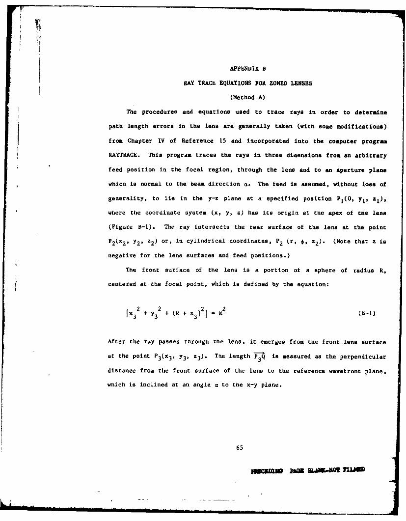
The procedures and equations used to trace rays in order to determine

path length errors in the lens are generally taken (with some modifications)

from Chapter IV of Reference 15 and incorporated into the computer program

RAYTKACE. This program traces the rays in three dimensions from an arbitrary

feed position in the focal region, through the lens and to an aperture plane

whicn is normal to the beam direction a. The feed is assumed, without loss of

generality, to lie in the y-z plane at a specified position PI(O, y1, Z1 ),

where the coordinate system (x, y, z) has its origin at the apex of the lens

(Figure B-I). The ray intersects the rear surface of the lens at the point

P2 (x2, Y2 . z2 ) or, in cylindrical coordinates, P2 (r, *, zZ). (Note that z is

negative for the lens surfaces and feed positions.)

The front surface of the lens is a portion of a sphere of radius R,

centered at the focal point, which is defined by the equation:

[x 32 + y3

2 + (K + z3 )2] - L (-I)

After the ray passes through the lens, it emerges from the front lens surface

at the point P3(x3, Y3, z3). The length P is measured as the perpendicular

distance from the front surface of the lens to the reference wavef ront plane,

which is inclined at an angle a to the x-y plane.

65

-FKM PAWI RAWk-MO f

Equations (B-2) through (B-10) may be derived from the geometry of Figure

B-1 and Snell's Law. The equations of the incident ray segment PIP 2 from the

feed to the rear surface of the lens are given by

XI - x2 YI - Y2 ZI - z2

L M

where L, M, N are directional cosines:

x2 l - - Y z2 -Z

L = 2 , M M t2 , N - I (B-3)

ad l 2 - Pp- 2 2 )2 _ 2

and it I 1I =2 (x2 x1)2 + (Y2 - Yd + (z2 z

Each zone of the rear lens surface is represented by a polynomial in r2

in the parametric form of Eq. B-4 (note change from y2 in Appendix A to r2),

1 2 4 6 8F Fn(r 'z2) = c l n r + b 4n r +b r + b8nr - (z2 + g J O,

n-I,2,3,...N

(Eq. 4.33 of Ref. 15)(B-4)

where n is the zone number, corresponding to the given value of r.

The tangent plane at the point P2 on the rear lens surface is defined by the

angles:

r r) 2 2 2 1/2 (1-5),(IF) + (IF +(I

(Eq. 4.24 of Ref. 15)

66

2F w N

C, z

L 00C

6U) Z C -z 500

a-J

zw

00

LA.L

C.)C-

CXXXd-eN 41~

673

where

3F 2 4 6+- 6 bC n r + 8 b r x2 fn x 2 Fx

ax (cln+ 4b 4nr +6n +8 8nr) 2 x&F

3F

T-AF -Hya y n 2

3F+ F) -1

y yAlso :

x2 2 + )1/2F T (F x + Fy +1

Then:

a F /FT, r - Fy/FTYr I/FT (B-6)

The angle, I, between the ray segment P " and the normal to the tangent

plane at P2 is given by:

cos I - arL + 0r1 + yrN (Eq. 4.17 of ref. 15) (B-7)

The angle of refraction ',n at P2 is determined from Snell's law:

Cos ' 1 2 _ - I)} 1/2 (Eq. 4.17 of ref.15) (B-8)

The directional cosines LI, M', N' of the ray segment P2P3 at point P2

are given by:

68

p Lw - L K r (Eq. 4.2 of Ref. 15) (B-9)

1A M' - M K 0 r

PN' - a r

where K = cos cosI. (Eq. 4.3 of Ref. 15). (B-10)

The intersection coordinates P3 (x 3 , Y3, z3 ) of ray segment - at the front

lens surface are determined by first calculating the intercept point

PO (X0, Yo) of this ray with a transfer plane which is perpendicular to the

axis of symmetry (z axis) and passes through the apex of the lens; the ray is

then backtracked along P2P from P0 to P3 on the spherical lens surface. (See

Section 4.3 of Reference 15 for details). The coordinates x0 , y0 are given

by:

~L '

x =x 2 -. (Eq. 4.4 of Ref. 15) (B-1l)

o- y2 - T (z2)

We next calculate

v--(x 2 + y ) (Eq. 4.9 of Ref. 15) (B-12)

1 - N' +k(L' x° + M' yo) (Eq. 4.10 of Ref. 15) (B-13)

69

and

AV (Eq. 4.12 of Ref. 15) (1-14)

U + / + V/R

(A is the negative value of line segment PoP 3.)

Then:

x3 = L'A + x (Eq. 4.5 of Ref. 15) (1-15)

Y3 - M'A + yo

Z3 = N'A

We have now calculated the coordinates of P1, P2 , and P3. The lengths of

ray segments PIP 2 , 2P-3 , and P30 can then be obtained from the relations:

-1% - tan-(yI/zl) (B-16)

ye - tan-1 (23/y3) (B-17)

= "y + % (B-18)

Also

Y2 - r sin, (B-19)

x2 - r co * (B-20)

70

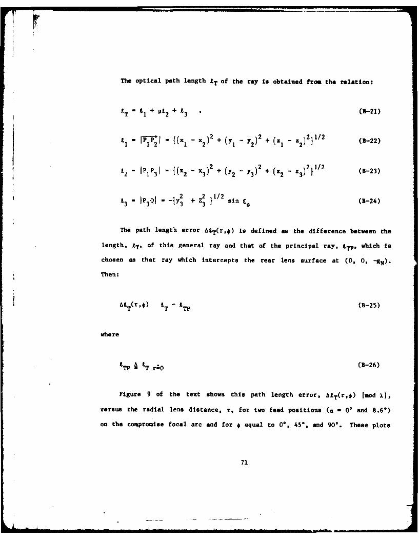
The optical path length IT Of the ray Is obtained from the relation:

I T I + 2 + 3 .(-1

12 P - R - x )2+ (yI- y 2+ z - z221/2 (B-22)1 22y 22 (1 2)

L2 1 IP 3I - {(x2 - 3)'2 + (y2 - y3) +(-z)2 2 1/2 (B-23)

£3 IP Q1 -1y2 +z2 1/2 sn(B-24)

The path length error AIT(r,f) is defined as the difference between the

length, IT, of this general ray and that of the principal ray, tLp, vhich Is

chosen as that ray which Intercepts the rear lens surface at (0, 0, -gN)-

Then:

AL~r*) f -L(B-25)T T TP

where

ITP I T r!0 (B-26)

Figure 9 of the text shows this path length error, AtT(r,#) [mod A.

versus the radial lens distance, r, for two feed positions (a - 0* and 8.6*)

on the compromise focal arc and for *equal to 0% 45% and 90%. These plots

71

were obtained from the computer program RAYTRACE which incorporated the

equations listed in this Appendix. The RAYTRACE program was also used for the

phase constant, 8(r,#), as input to the programs for calculating radiation

patterns and gain of the lens antennas (Appendix C) where

B(r, ) " 2w UT(r,#)/X • (-27)

72

APPENDIX C

CALCULATION OF GAIN AND .ADIATION PATTERNS OF ZONED LENS

(Nethod A)

A computer program was generated for calculating the directive gain and

radiation patterns of the leas antenna, based upon Eqs. 29 and 32 of the

text. This section presents details of these calculations:

Equation 32 for the antenna gain G (a) is repeated here for convenience:

f r dr d' G(aL) -[B/XZ( a ( 32)f [ (r,*) 12 r dr

This equation represents an integration of the near fields over the lens

aperture. However, we will take the integration over the projection of the

lens aperture upon that wavefront aperture plane which Is perpendicular to the

beam direction. Although this projected area is elliptical rather than

circular in cross-section, this distortion will be slight if the beam tilt

angle Is small so that the projected area can be assumed to be of the same

size as the lens aperture. Additionally, the obliquity factor is assumed to

be negligible in the radiation integral, and a thin lens approximation is made

in which the cylindrical coordinates (r,*) of the ray at the rear lens surface

are approximated by those (r,*) in the tilted coordinate system (X',Y',Z') of

the projected aperture plane (Figure B-I). Under these conditions, Eq. 29

will still be applicable.

73

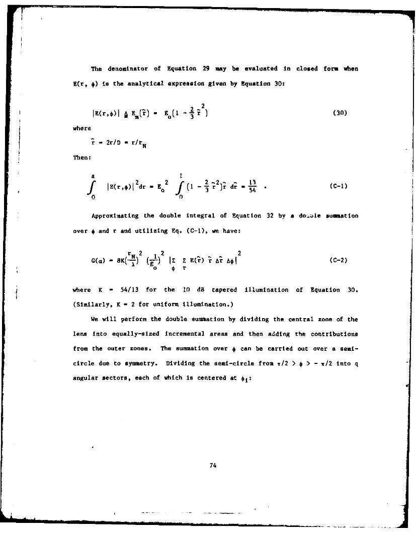
The denominator of Equation 29 may be evaluated in closed form when

E(r, *) is the analytical expression given by Equation 30:

2

where

re 2riD - r/rN

Then:

a 1t02 2 2'r2r 13

E(r,f)l dr - E f (1 -- )r dr -(C-)f 0 T

Approximating the double integral of Equation 32 by a do,:le summation

over # and r and utilizing Eq. (C-1), we have:

rN 2 12 20(Q) - 8K(- 7 ) (-) IZ E E(i) A AI (C-2)

o r

where K - 54/13 for the 10 dB tapered illumination of Equation 30.

(Similarly, K - 2 for uniform illuminatlon.)

We will perform the double summation by dividing the central zone of the

lens into equally-sized Incremental areas and then adding the contributions

from the outer zones. The summation over f can be carried out over a semi-

circle due to symmetry. Dividing the semi-circle from w/2 > * > - w/2 into q

angular sectors, each of which is centered at I:

74

momm-

-[ -2l - - 1) C-3)

where A* - w/q i 1,2,3,...,q

Similarly, the central zone is divided into radial annuli of equal area

for which each mean radius rk is located at

[k + /2 (k-I-/24)

and

c) 1/2 /-I 1

,rK =- [C) / C -- )/]r c k-I,2,3,...,p

re " rc/rN

rN , outer radius of lens

re - radius of central zone.

1

For the outer zones, the radial width of each annulus is arbitrarily made

equal to the width of the zone. Equation C-2 for the antenna gain G(a) can

then be written (omitting several algebraic steps):

S2 - 2r 2 r

G( ) - A{(-- + 2] + c • + F] 2 (C-5)p

where

22 rN 2

A2q

75

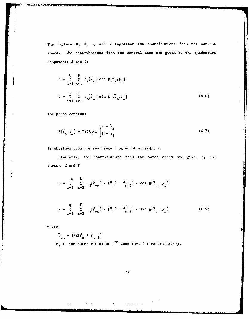
The factors B, C, D, and F represent the contributions from the various

zones. The contributions from the central zone are given by the quadrature

components 6 and D:

q pB E "~LI(k) CosBrk)i-i k-I

q pE E s (k in ~'i)(C-6)

i=i k-I

The phase constant

= k (c-7)

is obtained from the ray trace program of Appendix B.

Similarly, the contributions from the outer zones are given by the

factors C and F:

q Ni- rn E(on) • (rn - n 1 ) • cos a( on,,i)iffl a.f2

q NF E i . E. (io ) - rn - )n sin 6( on,,d ) (C-9)

i-1 n"2

where

ol " 2(n + n-)

rn is the outer radius ot nt h zone (n-I for central zone).

76

An obvious modification of 4q. (C-5) for greater accuracy in evaluating

G(a) is to use a finer grid for the contributions from the outer zones.

However, the results obtained for the experimental lens agreed within about

0.1 dB with those obtained from other programs, so this was not judged to be

necessary.

The far-field amplitude F(O', ') is calculated from Eq. 26, which is an

integral of similar form to that for G(a), except that the phase constant

8(r,$) m-st be replaced by B (r,o,6',') where 6' and *' are the polar

coordinates for the radiated field and

2r Na(rk'OiJ + (-y--) [rk sin 0' cos(' -

The tecniques for replacing the double integrals by double summations then

follow the previous procedures.

77

REFERENCES

1. W. C. Cummings, P. C. Jain, and L. J. Ricardi, "Fundamental PerformanceCharacteristics that Influence EHF MILSATCOM Systems," IEEE Trans. Commun.COM-27, 1423 (1979), DDC-AD-A084591/7.

2. L. J. Ricardi, "Communication Satellite Antennas," Proc. IEEE 65, 356(1977), DDC-AD-A063415/4.

3. J. F. Ramsay, "A Universal Scanning Curve for Wide-Angle Mirrors andLenses," Marconi Review, XVIII, 150-159 (1Q56).

4. J. F. Ramsay and J. A. C. Jackson, "Wide-Angle Scanning Performance ofMirror Aerials," Marconi Review, XIX, pp. 119-140 (1956).

5. E. A. Ohm, "A Proposed Multiple-Beam Microwave Antenna for Earth Stationsand Satellites," Bell Sys. Tech. J., 53, 1657-1665 (1974). (Alsoreprinted in Electromagnetic Horn Antennas, A. W. Love, Ed. (IEEE Press,New York, 1976) p. 281.

6. H. Jasik, Antenna Engineering Handbook, (McGraw-Hill, New York 1961),p. 14-6.

7. T. C. Cheston and D. H. Shinn, "Scanning Aberrations of Radio Lenses,"Marconi Review, XV, 174-184 (1952).

8. D. H. Shinn, "The Design of a Zoned Dielectric Lens for Wide AngleScanning," Marconi Review, XVIII, 37-47 (1955).

9. M. Born and E. Wolf, Principles of Optics, (Pergamon Press, New York,1964), p. 211.

10. R. H. Clarke and J. Brown, "Diffraction Theory and Antennas," Section7.2.3, Eq. 7.48, (Halsted Press [Division of Wiley & Sons], 1980), p. 196.

11. P. D. Potter, "A New Horn Antenna With Suppressed Sidelobes and EqualBeamwidths," Microwave, XI, 71-78 (1963). (Also reprinted inElectromagnetic Horn Antennas, A. W. Love, Ed. (IEEE Press, New York

1976), p. 201.)

12. R. H. Turrin, "Dual Mode Small-Aperture Antennas," IEEE Trans. AntennasPropag. AP-15, 307 (1967). (Also reprinted in Electromagnetic HornAntennas, A. W. Love, Ed. (IEEE Press, New York, 1976), p. 214.)

13. M. I. Skolnik, Radar Handbook," (Mcgraw-Hill, New York, 1970) p. 9.

78

REFERENCES (cont'd)

14. F. G. Friedlander, "A Dielectric-Lens Aerial for Wide-Angle BeamScanning," Inst. Elec. Eng.,_93, Pt. 3A, 658-662 (1946).

15. W. Welford, Aberrations of the SymmetrIcal Optical System (Academic Press,

New York 1914).

16. J. J. Lee, "Numerical Methods Make Lens Antennas Practical," Microwaves21, 81-84 (1982).

79

AcKnowledgments

The author acknowledges the support of John Russo, who conducted the

antenna measurements, and Dennis Weikle who provided the engineering

development of the lens antenna model. He also appreciates the assistance of

Dr. Andre Dion who supplied the computer programs which were used for the

Method B analysis of lens performance and David Besse who programmed the lens

design and Method A equations.

80

UNCLASSIFIED

SECURITY CLASSIFICATIONI OF THIS PAGE lVhon Deft Em.4 EAs,.d)1tioREPORT DOCUMENTATION PAGE woawuF znc oa

1. MPRTWINE ACCESSION SO. . UW110liS CATMI

TIME and subtide) G.T OM &W 9UI INl IU

EHF Dielectric Lens Antenna for Satellite Technical Report

Communication Systems ~ Inoneu.NPUI__________________________________________ Technical Report 620

7. AtIT111011(s S. COBTRACT O NT w UNB(F)

Walter Rotman F19628-80-C-0002

9. PERFORMNG ORGAIuZATOE NAME *10 ADORES$ it. PROM ELEMENT NOECT TANKLincoln~~~AN Laoao& MIT M WONK UNIT SUMERUS

PLi.coxn 73oaoyMIT Program Element Nos. 63431FP.O. ox 73and 33601F

Lexington, MA 02173-0073 Project Nos. 2029 and 643011I. CONTRaLUNs OFFICE NAME AND ADDRESS 12. REPORT DATE

Air Force Systems Command, UJSAF 3 January 1983Andrews AFB 13. NUMER OF PAGESWashington, DC 20331 90

14. MONITORING AGENCY NME & A"DRESS (if different from Controlling Office.) 1S. SECtNNTY CLASS. (of "bS repao

UnclassifiedElect conir Systems DivisionHanscom AFB, MA 01731 [iao. DECLASSIFICATION DOWUSMONO SCIIEDIKE

16. DISTISUTION STATEMKENT (of this Report)

Approicd for pulblic release, distribution unlimited.

17. DISTRIBUTION STATEENT (of the oabutract entered in Block 20. if different froms Report)

11. SUPtENETANY NOTES

None

Is. KEY wowOs (Continue on reverse side if necs-ary and identify byv block nmber)

EHF technology millimeter wave antennadielectric lens antenna multi-beam antennasatellite communication

26. ANSTRACT (C ontiunhe on reve rse side if nereuorv and identiy by block numsber)l

Dielectric lens antennas are applicable to the design of multiple-beam antenna (MBA) systems on EHF communica-tion satellites. Advantages include excellent wide angle scanning properties and elimination of feed blockage. This re-port describes an experimental 90A dia. zoned dielectric lens, operating at 44 GB:, which wast fabricated and tested inorder to estimate the performance of a dielectric lens; MBA. Measurements showed that the lens generated a beam witha half-power beamwidth (H-PBW) of 0.70 which could be steered over a total mean angle of 18* (corresponding to theearth's field-of-view from a geosynchronous satellite) with a scanning loss of less than I dB and a gain in excess of 47 dBimeaured at the suab-satellite point over a 5% bandwidth. A theoretical analysis of the radiation characteristics of thelens antenna. using ray tracing and geometric optics techniques, gave excellenrt agreement with the measurements. Sim-plified design equations were developed to facilitate evaluastion and development of lens antenna systems of this type.

DO 1473 EOM0R OF I1NOV U13I OBSOLETE UNCLASSIFIEDI J0 73SECU~rY CLASSIFI1CATION OF THIS PAGE (When DamsNaes*