Peerless Pump Company 2005 Dr. M.L. King Jr. Street, P.O. Box 7026, Indianapolis, IN 46207-7026, USA Telephone: (317) 925-9661 Fax: (317) 924-7338 www.peerlesspump.com www.epumpdoctor.com

1 Revised 07/06

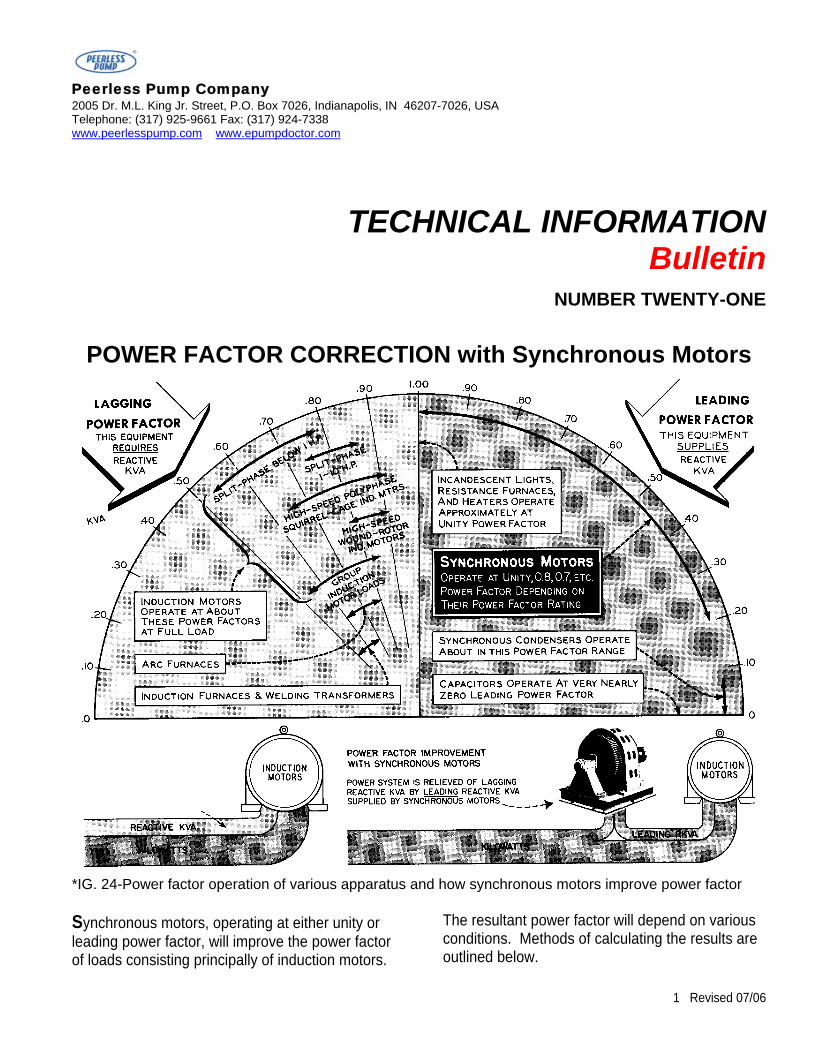
*IG. 24-Power factor operation of various apparatus and how synchronous motors improve power factor

Synchronous motors, operating at either unity or leading power factor, will improve the power factor of loads consisting principally of induction motors.

The resultant power factor will depend on various conditions. Methods of calculating the results are outlined below.

TECHNICAL INFORMATION Bulletin

NUMBER TWENTY-ONE

POWER FACTOR CORRECTION with Synchronous Motors

THE GRAPHIC METHOD FOR POWER FACTOR CALCULATIONS

2 Revised 07/06

3 Revised 07/06

The graphical method illustrated in Figure 25 will be discussed first. A sheet of cross section paper with 1 inch squares is usually convenient to work with. Using O as a center, scribe the quadrant of a circle (Power Factor Circle Number 1) to any convenient scale, so the base can be marked off in tenths. Lay off kilowatts along the same base line to any convenient scale. Lagging power factor is considered negative so for an initial lagging condition use the lower right hand quadrant. Now we can represent an initial load and power factor condition by a line, which then becomes a vector. Assume a load of 600 KW at 0.7 lagging power factor. Draw a power factor line, starting at 0 and passing through the power factor circle at L, which is the point directly below 0.7 on the power factor base line and which then represents 0.7 lagging power factor. Draw a vertical line BC from the 600 KW load point on the kilowatt base line to the 0.7 lagging power factor line. Then OC represents the existing condition. OB = KW = 600; OC = KVA = 856; BC = RKVA = -610. Assume that we are to add Bhp load at 1.0 power factor to the above. With C as a new center draw Power Factor Circle Number 2, preferably to the same scale as Number 1. With an assumed motor efficiency of 92% the kilowatt added input equals 250 x .746 / .92 = 203. This would be represented by CD; then OD represents the resultant condition. OE = KW = 803; OD = KVA = 1015; ED = RKVA = -610, which is unchanged. Line OD projected to the original power factor circle intersects it at M, indicating a new power factor of .79; this may be checked since KW / KVA = -803/1015 = .792 lag If, however, we add a 0.8 leading power factor motor instead of the unity power factor motor mentioned above, there will be a slight but insignificant increase in KW as the efficiency would be slightly reduced. Assume it is unchanged. Still using power factor circle Number 2, draw a line CN to intersect the power factor circle at a point directly above 0.8, this indicating a 0.8 leading power factor condition. Since the kilowatt load is assumed unchanged the new resultant is represented by intersection of KW line DE and 0.8 leading power factor line is determined by OF projected to the power factor

circle at P, indicating a value of .87 lagging. Now OE = KW = 803, OF = KVA = 925; EF = RKVA = -455. We can check this since KW / KVA = PF and 803 / 925 = .868. Conversely if the initial conditions, the desired final power factor and the load to be added are known, it is possible to determine the power factor at which the added load must operate to obtain the desired results. Table of Tangents Method Another method of calculating power factor is that of using the Reactive KVA table (See Table on next page). It is not necessary to draw any power factor circles, but it is generally advantageous to make a rough sketch showing the added loads as you go along. The table is based on the power triangle shown in Figure 26. For each value of power factor there is a corresponding ration of RKVA / KW. A leading KVA would be shown as positive or above the KW line and lagging RKVA as negative. Referring to the previous example of 600 at 0.7 lagging power factor, from the table we find 1.02 RKVA per KW. This will be negative since the power factor is lagging. OB = KW = 600; BC = RKVA = 600 x -1.02 = -612; OC = KVA = 600 / 0.7 = 857. To this we can add a 250 HP load, which is 203 KW at 1.0 power factor. This would be represented by CD, making the resultant OD. This totals as follows:

KW KVAR Original load 600 -612 Added load 203 0 Resultant 803 -612

Thus the ratio of RKVA / KW = -612 / 803 = -0.762. Interpolating in the table of tangents we find this equivalent to 0.795 lagging power factor. This checks the graphical solution of the same problem. If instead of the unity power factor motor we apply a motor at 0.8 leading power factor, we would first determine its KW and RKVA. Assume the KW unchanged at 203.

From the table of tangents we find a ratio of RKVA / KW at 0.8 power factor to be .75; thus we would have 203 x .75 = 152 RKVA; this would be positive since it is leading. Totals would then be; at condition OF:

KW RKVA Original load 600 -612 Added load 203 +152 Resultant 803 -460

Thus the ratio of RKVA / KW for the resultant load is -406 / 803 = -.572. Interpolating in table X we find this corresponds to a power factor of .868 lag. This also checks with the previous graphical solution. Any desired number of loads can be added by totalizing the KW and RKVA values, keeping in mind the proper sign for leading and lagging conditions.

The Table of TANGENTS •••

FIGURE 26. In using Table of Tangents method, a vector sketch of loads as shown

above will help check results.

The Table of Tangents at the right is based on the trigonometric relationships of the power triangle. Referring to the vector diagram above, the cosine of angle BOC equals OB / OC. The tangent of angle BOC equals BC / OR. In this power triangle:

OB = KW OC = KVA BC = KVAR SYNCHRONOUS MOTOR Correction at Part Load… In many cases, motors are operated on cyclic duty where they will be operated at substantially less than rated load for considerable periods of time. In the case of induction motors this is usually detrimental to power factor as the lagging reactive KVA component decreases only slightly with decrease in load, while the kilowatt component decreases almost in direct ratio to the load. This results in a high ratio of reactive KVA to KW and a low power factor at light loads.

However a synchronous motor will operate at a lower leading power factor and deliver more leading reactive KVA at part load, if the excitation is unchanged, than it will at full load. This is an important and valuable characteristic and is often made use of on cyclic loads. In some cases it may be desired to calculate the reactive KVA at some known load and power factor:

Ratio Ratio Power Ratio Power RatioFactor KVAR/KW Factor KV AR/KW Factor KV

AR/KW 1.00 .000 .80 .750 .60 1.333 .99 .143 .79 .776 .59 1.369 .98 .203 .78 .802 .58 1.405 .97 .251 .77 .829 .57 1.442 .96 .292 .76 .855 .56 1.480 .95 .329 .75 .882 .55 1.518 .94 .363 .74 .909 .54 1.559 .93 .395 .73 .936 .53 1.600 .92 .426 .72 .964 .52 1.643 .91 .456 .71 .992 .51 1.687 .90 .484 .70 1.020 .50 1.732 .89 .512 .69 1.049 .49 1.779 .88 .540 .68 1.078 .48 1.828 .87 .567 .67 1.108 .47 1.878 .86 .593 .66 1.138 .46 1.930 .85 .620 .65 1.169 .45 1.985 .84 .646 .64 1.201 .44 2.041 .83 .672 .63 1.233 .43 2.100 .82 .698 .62 1.266 .42 2.161 .81 .724 .61 1.299 .41 2.225

4 Revised 07/06

5 Revised 07/06

RKVA = (0.746 x Bhp) / (Eff. x PF) x 1 - (PF)2 Where RKVA = Reactive KVA Bhp = Horsepower output Eff = Operating efficiency PF = Power factor expressed as a decimal.

Note that the reactive KVA may be either leading or lagging.

Occasionally synchronous motors may be operated at part load for considerable periods of time and it will be desirable to estimate the power factor correction available under those conditions. Refer to Figure 27 below. From these curves it is possible to determine the approximate leading KVA in percent of rated horsepower for various conditions of load and for motors designed for

various power factor values at full load. For instance, a 250 Bhp, 0.8 power factor motor operating at 100% load will deliver approximately 60% of its horsepower rating, or 250 x .6 = 150 leading RKVA to the system. In each case the motor is considered operating at full rated excitation from zero to 100% load. Above 100% load the excitation is reduced so as to maintain full rated armature amperes. Obviously if the excitation is not reduced the motor will draw much more KVA and deliver more leading reactive KVA. However the rated stator amperes will be exceeded and the motor would overheat under that condition. It must be borne in mind that the pull-out torque is reduced with reduction in excitation. To handle occasional peak overloads may require full excitation.