technical appendix to the book « capital et ideology
TRANSCRIPT
1
Technical appendix to the book « Capital et ideology » Thomas Piketty
Harvard University Press - March 2020 http://piketty.pse.ens.fr/ideology
Figures and tables presented in this book
Introduction Figure 0.1. Health and education in the world, 1820–2020 Figure 0.2. World population and income, 1700–2020 Figure 0.3. The rise of inequality around the world, 1980–2018 Figure 0.4. Inequality in different regions of the world in 2018 Figure 0.5. The elephant curve of global inequality, 1980–2018 Figure 0.6. Inequality, 1900–2020: Europe, United States, and Japan Figure 0.7. Top income tax rates, 1900–2020 Figure 0.8. Parental income and university access, United States, 2014 Figure 0.9. Transformation of political and electoral conflict, 1945–2020: Emergence of a multiple-elites party system, or great reversal?
Part One. Inequality Regimes in History Chapter 1. Ternary Societies: Trifunctional Inequality Figure 1.1. The structure of ternary societies: Europe-India, 1660–1880 Chapter 2. European Societies of Orders: Power and Property Figure 2.1. Population shares in French ternary society, 1380–1780 (as percentage of total population) Figure 2.2. Share of nobility in Paris inheritances, 1780–1910 Figure 2.3. The Church as property-owning organization, 1750–1780 Table 2.1. Clergy and nobility in France, 1380–1780 (as percent of total population) Table 2.2. Clergy and nobility in France, 1380–1780 (as percent of total adult male population)

2
Chapter 3. The Invention of Ownership Societies Table 3.1. Progressive tax proposals in eighteenth-century France Chapter 4. Ownership Societies: The Case of France Figure 4.1. The failure of the French Revolution: The rise of proprietarian inequality in nineteenth-century France Figure 4.2. The distribution of property in France, 1780–2015 Figure 4.3. The distribution of income in France, 1780–2015 Table 4.1. Composition of Parisian wealth in the period 1872–1912 (in percent) Chapter 5. Ownership Societies: European Trajectories Figure 5.1. The weight of the clergy in Europe, 1530–1930 Figure 5.2. The weight of the nobility in Europe, 1660–1880 Figure 5.3. Evolution of male suffrage in Europe, 1820–1920 Figure 5.4. Distribution of property in the United Kingdom, 1780–2015 Figure 5.5. Distribution of property in Sweden, 1780–2015 Figure 5.6. Extreme wealth inequality: European ownership societies in the Belle Époque, 1880–1914 Figure 5.7. Income inequality in European ownership societies in the Belle Époque, 1880–1914
Part Two. Slave and Colonial Societies Chapter 6. Slave Societies: Extreme Inequality Figure 6.1. Atlantic slave societies, eighteenth and nineteenth centuries Figure 6.2. A slave island in expansion: Saint-Domingue, 1700–1790 Figure 6.3. Proportion of slaves in the United States, 1790–1860 Figure 6.4. The rise and fall of Euro-American slavery, 1700–1890 Table 6.1. The structure of the slave and free population in the United States, 1800-1860 Chapter 7. Colonial Societies: Diversity and Domination Figure 7.1. The proportion of Europeans in colonial societies

3
Figure 7.2. Inequality in colonial and slave societies Figure 7.3. Extreme inequality in historical perspective Figure 7.4. The top centile in historical and colonial perspective Figure 7.5. Extreme inequality: Colonial and postcolonial trajectories Figure 7.6. Subsistence income and maximal inequality Figure 7.7. The top centile in historical perspective (with Haiti) Figure 7.8. Colonies for the colonizers: Inequality of educational investment in historical perspective Figure 7.9. Foreign assets in historical perspective: The Franco-British colonial apex Chapter 8. Ternary Societies and Colonialism: The Case of India Figure 8.1. Population of India, China, and Europe, 1700–2050 Figure 8.2. The religious structure of India, 1871–2011 Figure 8.3. The evolution of ternary societies: Europe-India 1530–1930 Figure 8.4. The rigidification of upper castes in India, 1871–2014 Figure 8.5. Affirmative action in India, 1950–2015 Figure 8.6. Discrimination and inequality in comparative perspective Table 8.1. The structure of the population in Indian censuses, 1871–2011 Table 8.2. The structure of high castes in India, 1871–2014 (percentage of population) Chapter 9. Ternary Societies and Colonialism: Eurasian Trajectories Figure 9.1. State fiscal capacity, 1500–1780 (tons of silver) Figure 9.2. State fiscal capacity, 1500–1850 (days of wages) Figure 9.3. The evolution of ternary societies: Europe-Japan 1530–1870
Part Three. The Great Transformation of the Twentieth Century Chapter 10. The Crisis of Ownership Societies Figure 10.1. Income inequality in Europe and the United States, 1900–2015 Figure 10.2. Income inequality, 1900–2015: The diversity of Europe Figure 10.3. Income inequality, 1900–2015: The top centile Figure 10.4. Wealth inequality in Europe and the United States, 1900–2015 Figure 10.5. Wealth inequality, 1900–2015: The top centile Figure 10.6. Income vs. wealth inequality in France, 1900–2015

4
Figure 10.7. Income versus wealth in the top centile in France, 1900–2015 Figure 10.8. Private property in Europe, 1870–2020 Figure 10.9. The vicissitudes of public debt, 1850–2020 Figure 10.10. Inflation in Europe and the United States, 1700–2020 Figure 10.11. The invention of progressive taxation, 1900–2018: The top income tax rate Figure 10.12. The invention of progressive taxation, 1900–2018: The top inheritance tax rate Figure 10.13. Effective rates and progressivity in the United States, 1910–2020 Figure 10.14. The rise of the fiscal state in the rich countries, 1870–2015 Figure 10.15. The rise of the social state in Europe, 1870–2015 Figure 10.16. Demography and the balance of power in Europe Chapter 11. Social-Democratic Societies: Incomplete Equality Figure 11.1. Divergence of top and bottom incomes, 1980–2018 Figure 11.2. Bottom and top incomes in France and the United States, 1910–2015 Figure 11.3. Labor productivity, 1950–2015 (2015 euros) Figure 11.4. Labor productivity in Europe and the United States Figure 11.5. The fall of the bottom 50 percent share in the United States, 1960–2015 Figure 11.6. Low and high incomes in Europe, 1980–2016 Figure 11.7. Low and high incomes in the United States, 1960–2015 Figure 11.8. Low incomes and transfers in the United States, 1960–2015 Figure 11.9. Primary inequality and redistribution in the United States and France Figure 11.10. Minimum wage in the United States and France, 1950–2019 Figure 11.11. Share of private financing in education: Diversity of European and American models Figure 11.12. Growth and inequality in the United States, 1870–2020 Figure 11.13. Growth and progressive taxation in the United States, 1870–2020 Figure 11.14. Growth and inequality in Europe, 1870–2020 Figure 11.15. Growth and progressive tax in Europe, 1870–2020 Figure 11.16. Composition of income in France, 2015 Figure 11.17. Composition of property in France, 2015 Figure 11.18. Inequalities with respect to capital and labor in France, 2015 Figure 11.19. Profile of tax structure in France, 2018 Chapter 12. Communist and Postcommunist Societies
5
Figure 12.1. Income inequality in Russia, 1900–2015 Figure 12.2. The top centile in Russia, 1900–2015 Figure 12.3. The income gap between Russia and Europe, 1870–2015 Figure 12.4. Capital flight from Russia to tax havens Figure 12.5. Financial assets held in tax havens Figure 12.6. The fall of public property, 1978–2018 Figure 12.7. Ownership of Chinese firms, 1978–2018 Figure 12.8. Inequality in China, Europe, and the United States, 1980–2018 Figure 12.9. Regional inequality in the United States and Europe Figure 12.10. Inflows and outflows in Eastern Europe, 2010–2016 Chapter 13. Hypercapitalism: Between Modernity and Archaism Figure 13.1. Population by continents, 1700–2050 Figure 13.2. Global inequality regimes, 2018 Figure 13.3. Inequality in Europe, the United States, and the Middle East, 2018 Figure 13.4. Global inequality regimes, 2018: The bottom 50 percent versus the top 1 percent Figure 13.5. Inequality between the top 10 percent and the bottom 50 percent, 2018 Figure 13.6. Inequality between the top 1 percent and the bottom 50 percent, 2018 Figure 13.7. The global distribution of carbon emissions, 2010–2018 Figure 13.8. Top decile wealth share: Rich and emerging countries Figure 13.9. Top centile wealth share: Rich and emerging countries Figure 13.10. The persistence of hyperconcentrated wealth Figure 13.11. The persistence of patriarchy in France in the twenty-first century Figure 13.12. Tax revenues and trade liberalization Figure 13.13. The size of central bank balance sheets, 1900–2018 Figure 13.14. Central banks and financial globalization Table 13.1. The rise of top global wealth holders, 1987–2017
Part Four. Rethinking the Dimensions of Political Conflict Chapter 14. Borders and Property: The Construction of Equality Figure 14.1. Social cleavages and political conflict in France, 1955–2020 Figure 14.2. Electoral left in Europe and the United States, 1945–2020: From the party of workers to the party of the educated

6
Figure 14.3. Legislative elections in France, 1945–2017 Figure 14.4. The electoral left in France: Legislatives, 1945–2017 Figure 14.5. The electoral right in France: Legislatives, 1945–2017 Figure 14.6. Presidential elections in France, 1965–2012 Figure 14.7. The evolution of voter turnout, 1945–2020 Figure 14.8. Voter turnout and social cleavages, 1945–2020 Figure 14.9. Left vote by level of education in France, 1956–2012 Figure 14.10. The reversal of the educational cleavage in France, 1956–2017 Figure 14.11. The left and education in France, 1955–2020 Figure 14.12. Political conflict and income in France, 1958–2012 Figure 14.13. Political conflict and property in France, 1974–2012 Figure 14.14. The religious structure of the French electorate, 1967–2017 Figure 14.15. Political conflict and Catholicism in France, 1967–2017 Figure 14.16. Political conflict and religious diversity in France, 1967–1997 Figure 14.17. Political conflict and religious diversity in France, 2002–2017 Figure 14.18. Political attitudes and origins in France, 2007–2012 Figure 14.19. Borders and property: The four-way ideological divide in France Figure 14.20. The European cleavage in France: The 1992 and 2005 referenda Table 14.1. Political-ideological conflict in France in 2017: An electorate divided into four quarters Chapter 15. Brahmin Left: New Euro-American Cleavages Figure 15.1. Presidential elections in the United States, 1948–2016 Figure 15.2. Democratic vote by diploma, 1948–2016 Figure 15.3. The Democratic Party and education: United States, 1948–2016 Figure 15.4. The Democratic vote in the United States, 1948–2016: From the workers’ party to the party of the highly educated Figure 15.5. Political conflict and income in the United States, 1948–2016 Figure 15.6. Social cleavages and political conflict: United States, 1948–2016 Figure 15.7. Political conflict and ethnic identity: United States, 1948–2016 Figure 15.8. Political conflict and racial cleavage in the United States, 1948–2016 Figure 15.9. Political conflict and origins: France and United States Figure 15.10. Legislative elections in the United Kingdom, 1945–2017 Figure 15.11. Labour Party and education, 1955–2017 Figure 15.12. From the workers’ party to the party of the highly educated: The Labour vote, 1955–2017
7
Figure 15.13. The electoral left in Europe and the United States, 1945–2020: From the workers’ party to the party of the highly educated Figure 15.14. Political conflict and income in the United Kingdom, 1955–2017 Figure 15.15. Social cleavages and political conflict: United Kingdom, 1955–2017 Figure 15.16. Political conflict and religious diversity in the United Kingdom, 1964-2017 Figure 15.17. Political conflict and ethnic categories in the United Kingdom, 1979–2017 Figure 15.18. The European cleavage in the United Kingdom: The 2016 Brexit referendum Chapter 16. Social Nativism: The Postcolonial Identitarian Trap Figure 16.1. The reversal of the educational cleavage, 1950–2020: United States, France, United Kingdom, Germany, Sweden, and Norway Figure 16.2. Political cleavage and education, 1960–2020: Italy, the Netherlands, Switzerland, Canada, Australia, and New Zealand Figure 16.3. Political conflict and income in Poland, 2001–2015 Figure 16.4. Political conflict and education in Poland, 2001–2015 Figure 16.5. Catalan regionalism and income, 2008–2016 Figure 16.6. Catalan regionalism and education, 2008–2016 Figure 16.7. Legislative elections in India (Lok Sabha), 1962–2014 Figure 16.8. The BJP vote by caste and religion in India, 1962–2014 Figure 16.9. Congress party vote by caste and religion in India, 1962–2014 Figure 16.10. The left vote by caste and religion in India, 1962–2014 Figure 16.11. The BJP vote among the high castes, 1962–2014 Figure 16.12. The BJP vote among the lower castes, 1962–2014 Figure 16.13. The BJP and the religious cleavage in India, 1962–2014 Figure 16.14. The BJP vote by caste, religion, and state in India, 1996–2016 Figure 16.15. The politicization of inequality in Brazil, 1989–2018 Chapter 17. Elements for a Participatory Socialism for the 21st Century Table 17.1. Circulation of property and progressive taxation Figure 17.1. Inequality of educational investment in France, 2018 Table 17.2. A new organization of globalization: transnational democracy

10%15%20%25%30%35%40%45%50%55%60%65%70%75%80%85%90%
1015202530354045505560657075808590
1820 1840 1860 1880 1900 1920 1940 1960 1980 2000 2020
Figure 0.1. Health and education in the world, 1820-2020
Life expectancy at birth(all births combined)Life expectancy at birth(individuals reaching one-year)Literacy rate (%)
Interpretation. Life expectancy at birth worlwide increased from an average of 26 years in the world in 1820 to 72 years in 2020. Life expectancy for those living to age 1 rose from 32 years to 73 years (because infant mortality before age 1 decreased from 20% in 1820 to less than 1% in 2020). The literacy rate for 15-year-olds-and over worldwide rose from 12% to 85%. Sources and series: see piketty.pse.ens.fr/ideology.et

50 €
100 €
200 €
400 €
800 €
0,5
1,0
2,0
4,0
8,0
1700 1740 1780 1820 1860 1900 1940 1980 2020
Figure 0.2. World population and income, 1700-2020
World population(in billions inhabitants) (left axis)
Average income per month and perinhabitant (in euros 2020) (right axis)
Interpretation. World population and average national income increased more than tenfold between 1700 and 2020: population increased from about 600 million inhabitants in 1700 to over 7 billion in 2020; income, expressed in 2020 euros and in purchasing power parity, increased from barely 80€ per month per person in 1700 to 1000€ per month per person in 2020. Sources and series: voir piketty.pse.ens.fr/ideology.et

20%
25%
30%
35%
40%
45%
50%
55%
60%
1980 1985 1990 1995 2000 2005 2010 2015
Sha
re o
f top
dec
ile in
tota
l inc
ome
Figure 0.3. The rise of inequality around the world, 1980-2018
IndiaUnited StatesRussiaChinaEurope
Interpretation. The share of the top decile (the 10% highest incomes) in total national income ranged between 26% and 34% in 1980 in the different parts of the world and from 34% and 56% in 2018. Inequality increased everywhere, but the size of the increase varies greatly from country to country, at all levels of development. For exemple it was greater in the United States than in Europe (enlarged EU, 540 millions inhabitants), and greater in India than in China. Sources and series: see piketty.pse.ens.fr/ideology.et

0%
10%
20%
30%
40%
50%
60%
70%
Europe China Russia United States SubsaharanAfrica
India Brasil Middle East
Sha
re o
f top
dec
ile in
tota
l inc
ome
Figure 0.4. Inequality in the different regions of the world in 2018
Interpretation. In 2018, the share of the top decile (the 10% highest incomes) in national income was 34% in Europe (EU+), 41% in China, 46% in Russia, 48% in the United States, 54% in Subsaharan Africa, 55% in India, 56% in Brasil and 64% in the Middle East. Sources and series: see piketty.pse.ens.fr/ideology.012, le candidat de gauche (Hollande) obtient 47% des voix parmi les électeurs sans diplôme (en dehors du certificat d'études primaires), 50% parmi les diplômés du secondaire (Bac, Brevet, Bep, etc.), 53% parmi les diplômés du supérieur court (bac+2) en 2012, le candidat de gauche (Hollande) obtient 47% des voix parmi les électeurs sans diplôme (en dehors du certificat d'études primaires), 50% parmi

0%20%40%60%80%
100%120%140%160%180%200%220%240%
10 20 30 40 50 60 70 80 90 99 99,9 99,99
Cum
ulat
ed g
row
th o
f per
adu
lt re
al in
com
e 19
80-2
018
Percentile of the global distribution of per adult real income
Figure 0.5. The elephant curve of global inequality 1980-2018
Interpretation. The bottom 50% incomes of the world saw substantial growth in purchasing power between 1980 and 2018 (between +60% and +120%). the top 1% incomes saw even stronger growth (between +80% and +240%). Intermediate categories grew less. In sum, inequalitiy decreased between the bottom and the middle of the global income distribution, and increased between the middle and the top. Sources and series: see piketty.pse.ens.fr/ideology.et
The bottom 50% captured 12% of total growth
The top 1% captured 27% of total growth
Rise of emerging countries
Lower and middle classes of rich countries lag behind world growth Prosperity of the
top 1% from all countries

25%
30%
35%
40%
45%
50%
1900 1910 1920 1930 1940 1950 1960 1970 1980 1990 2000 2010 2020
Sha
re o
f top
dec
ile in
tota
l inc
ome
Figure 0.6. Inequality, 1900-2020: Europe, United States, Japan
United States
Europe
Japan
Interpretation. The share of the top decile (the top 10% highest incomes) in total national income was about 50% in Western Europe in 1900-1910, before decreasing to about 30% in 1950-1980, then rising again to more than 35% in 2010-2020. Inequality grew much more strongly in the United States, where the top decile share approached 50% in 2010-2020, exceeding the level of 1900-1910. Japan was in an intermediate position. Sources and series: see piketty.pse.ens.fr/ideology.et

0%
10%
20%
30%
40%
50%
60%
70%
80%
90%
100%
1900 1910 1920 1930 1940 1950 1960 1970 1980 1990 2000 2010 2020
Mar
gina
l tax
rate
app
lied
to th
e hi
ghes
t inc
omes
Figure 0.7. The top income tax rate, 1900-2020
United StatesBritainGermanyFrance
Interpretation. The top marginal tax rate applied to the highest incomes averaged 23% in the United States from 1900 to 1932, 81% from 1932 to 1980, and 39% from 1980 to 2018. Over these same periods, the top rate was 30%, 89% and 46% in Britain, 18%, 58% and 50%in Germany, and 23%, 60% and 57% in France. Fiscal progressivity was at its highest level in the middle of the century, especially in the United States and in Britain. Sources and series: see piketty.pse.ens.fr/ideology.et
20%
30%
40%
50%
60%
70%
80%
90%
100%
0 10 20 30 40 50 60 70 80 90
Rat
e of
acc
ess
to h
ighe
r edu
catio
n
Percentile of parental income
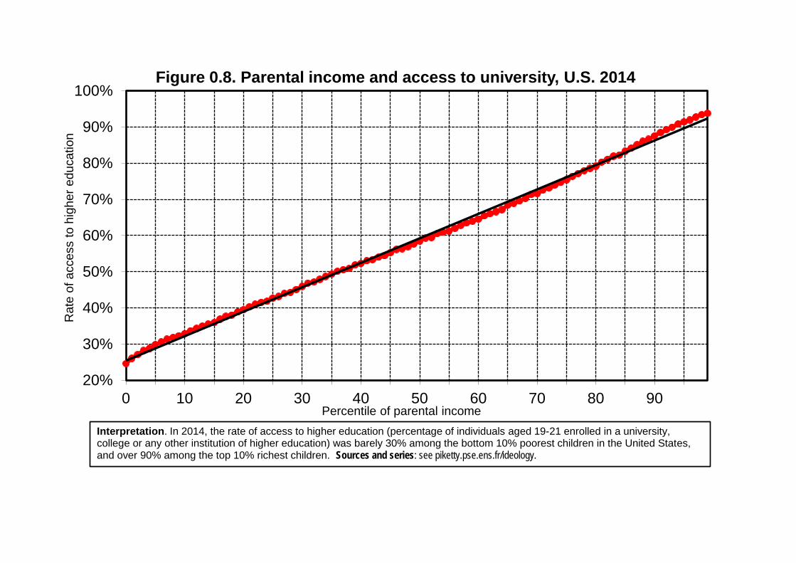
Figure 0.8. Parental income and access to university, U.S. 2014
Interpretation. In 2014, the rate of access to higher education (percentage of individuals aged 19-21 enrolled in a university, college or any other institution of higher education) was barely 30% among the bottom 10% poorest children in the United States,and over 90% among the top 10% richest children. Sources and series: see piketty.pse.ens.fr/ideology.et

-20%-16%-12%
-8%-4%0%4%8%
12%16%20%24%28%32%
1945 1950 1955 1960 1965 1970 1975 1980 1985 1990 1995 2000 2005 2010 2015 2020
Figure 0.9. Transformation of political and electoral conflict 1945-2020: emergence of a multiple-elites party system, or a great reversal?
U.S.: difference between % Democratic vote among the top 10% highest-education voters and the bottom 90% lowest-education voters (after controls)France: same difference with vote for left-wing parties
U.S.: difference between % Democratic vote among the top 10% highest-income voters and the bottom 90% lowest-income voters (after controls)France: same difference with % vote for left-wing parties
Interpretation. In the period 1950-1970, the vote for the Democratic party in the U.S. and for left-wing parties (Socialists, Communists, Radicals, Ecologists) in France was associated to voters with the lowest educational degrees and income levels; in the period 1980-2000, it became associated with the voters with the highest degrees; in the period 2010-2020, it is also becoming associated with the voters with the highest incomes (particularly in the U.S.). Sources and series: see piketty.pse.ens.fr/ideology. score 12 point
0%
1%
2%
3%
4%
5%
6%
7%
8%
9%
10%
11%
12%
France 1660 France 1780 Spain 1750 India 1880
Sha
re in
mal
e ad
ult p
opul
atio
n
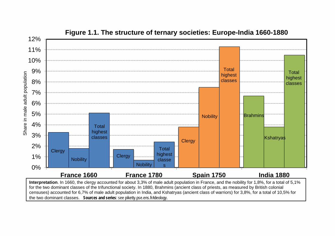
Figure 1.1. The structure of ternary societies: Europe-India 1660-1880
Clergy
Nobility
Total highestclasses
Brahmins
Kshatryas
Total highest classes
Interpretation. In 1660, the clergy accounted for about 3,3% of male adult population in France, and the nobility for 1,8%, for a total of 5,1% for the two dominant classes of the trifunctional society. In 1880, Brahmins (ancient class of priests, as measured by British colonial censuses) accounted for 6,7% of male adult population in India, and Kshatryas (ancient class of warriors) for 3,8%, for a total of 10,5% for the two dominant classes. Sources and series: see piketty.pse.ens.fr/ideology.012, le candidat de gauche (Hollande) obtient 47% des voix parmi les électeurs sans diplôme (en dehors du certificat d'études primaires) 50% parmi les diplômés du secondaire (Bac Brevet Bep etc ) 53% parmi les
Clergy
Clergy
Nobility
Nobility
Total highest classe
s
Total highest classes

0,0%
0,5%
1,0%
1,5%
2,0%
2,5%
3,0%
3,5%
4,0%
1380 1470 1560 1660 1700 1780
Figure 2.1. Population shares in French ternary society (1380-1780) (% total population)
Total clergy + nobilityNobilityClergy
Interpretation. In 1780, the nobility and the clergy accounted respectiviely for 0,8% and 0,7% of total French population, or a total of 1,5% for the two dominant orders and 98,5% for the third estate; in 1660, the nobility and the clergy accounted respectively for 2,0% and 1,4% of total population, or a total of 3,4% for the two dominant orders and 96,6% for the third estate. These proportions remained fairly stable between 1380 and 1660, followed by a sharp drop between 1660 and 1780. Sources and series: see piketty.pse.ens.fr/ideology.et

0%
5%
10%
15%
20%
25%
30%
35%
40%
45%
50%
55%
1780 1790 1800 1810 1820 1830 1840 1850 1860 1870 1880 1890 1900 1910
Figure 2.2. Share of nobility in Paris estates, 1780-1910Share of noble names in top 0,1%highest inheritancesShare of noble names in top 1%highest inheritancesShare of noble names in theaggregate value of inheritancesShare of noble names in the totalnumber of deceased individuals
Interpretation. The share of noble names among the top 0,1% highest inheritances in Paris dropped from 50% to 25% between 1780 and 1810, before rising to about 40%-45% during the period of censitory monarchies (1815-1848), and finally declining to about 10% in the late 19th century and early 20th century. By comparison, noble names have always represented less than 2% ofthe total number of deceased individuals between 1780 and 1910. Sources and series: see piketty.pse.ens.fr/ideology.et

0%
5%
10%
15%
20%
25%
30%
Spain 1750 France 1780 France 2010 U.S. 2010 Japan 2010
Figure 2.3. The Church as a property-owning organization 1750-1780
Interpretation. Around 1750-1780, the Church owned between 25% and 30% of total property in Spain and close to 25% in France (all assets combined: land, real estate, financial assets, including capitalisation of church tithes). By comparison, in 2010, the set of all non-profit institutions (including religious organizations, universities, museums, foundations, etc.) owned less than 1% of total property in France, 6% in the United States and 3% in Japan. Sources and series: see piketty.pse.ens.fr/ideology.012, le candidat de gauche (Hollande) obtient 47% des voix parmi les électeurs sans diplôme (en dehors du certificat d'études primaires), 50% parmi les diplômés du secondaire (Bac, Brevet, Bep, etc.), 53% parmi les
Share of Church in
total property
(all assets) (18th c.)
Share of non-profit institutions in total property (21th c.)

1380 1470 1560 1660 1700 1780
Clergy 1,4% 1,3% 1,4% 1,4% 1,1% 0,7%
Nobility 2,0% 1,8% 1,9% 2,0% 1,6% 0,8%
Total Clergy + Nobility 3,4% 3,1% 3,3% 3,4% 2,7% 1,5%
Third Estate 96,6% 96,9% 96,7% 96,6% 97,3% 98,5%
Total population (millions) 11 14 17 19 22 28
incl. Clergy (thousands) 160 190 240 260 230 200
incl. Nobility (thousands) 220 250 320 360 340 210
Interpretation: in 1780, the clergy and the nobility included respectively about 0,7% and 0,8% of total population in France, hence a total of 1,5% for the two dominant orders (about 410 000 individuals out of 28 millions). Sources and series: see piketty.pse.ens.fr/ideology.
Table 2.1. Clergy and nobility in France 1380-1780 (% of total population)

1380 1470 1560 1660 1700 1780
Clergy 3,3% 3,2% 3,3% 3,3% 2,5% 1,7%
Nobility 1,8% 1,6% 1,8% 1,8% 1,5% 0,7%
Total Clergy + Nobility 5,1% 4,8% 5,1% 5,1% 4,0% 2,4%
Third Estate 94,9% 95,2% 94,9% 94,9% 96,0% 97,6%
Adult male population (millions)
3,4 4,2 5,1 5,6 6,5 8,3
incl. Clergy (thousands) 110 130 160 180 160 140
incl. Nobility (thousands) 60 60 90 100 90 60
Table 2.2. Clergy and nobility in France 1380-1780 (% of adult male population)
Interpretation: in 1780, the clergy and the nobility included respectively about 1,7% and 0,7% of adult male population in France, hence a total of 2,4% for the two dominant orders (about 200 000 individuals out of 8,3 millions). Sources and series: see piketty.pse.ens.fr/ideology.
Multiple of average income Effective tax rate Multiple of average wealth Effective tax rate0,5 5% 0,3 6%20 15% 8 14%200 50% 500 40%
1300 75% 1500 67%
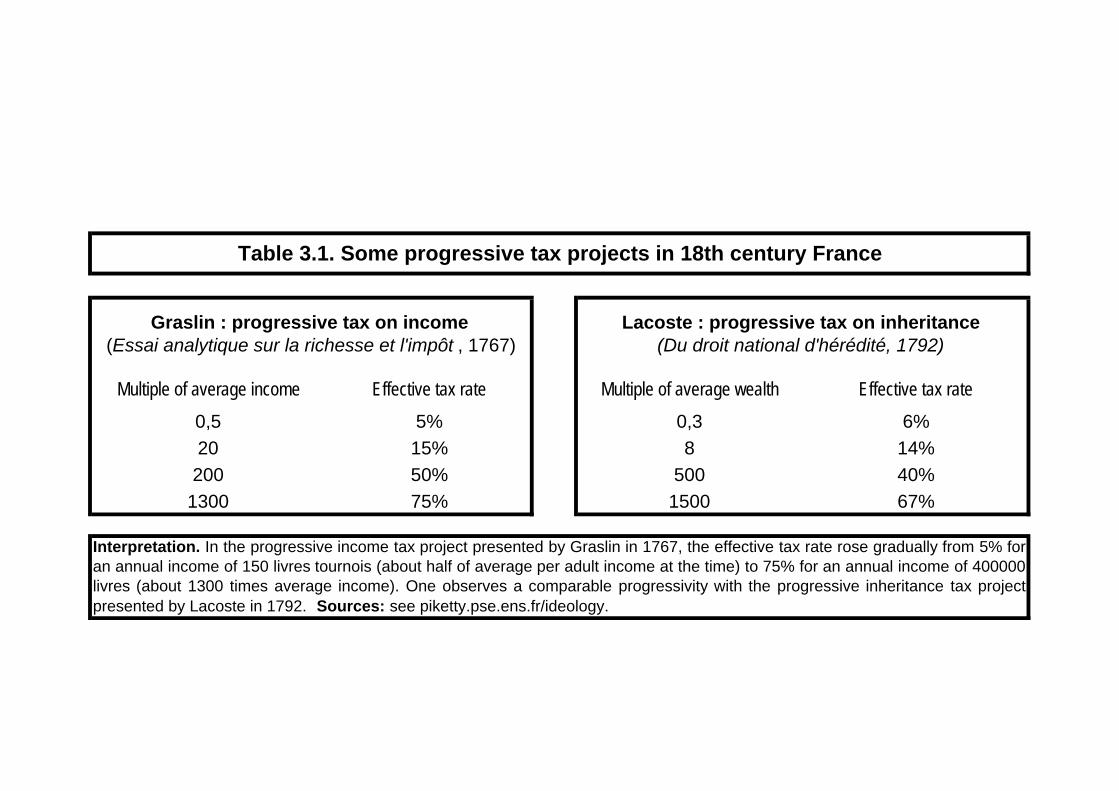
Table 3.1. Some progressive tax projects in 18th century France
Graslin : progressive tax on income (Essai analytique sur la richesse et l'impôt , 1767)
Lacoste : progressive tax on inheritance (Du droit national d'hérédité, 1792)
Interpretation. In the progressive income tax project presented by Graslin in 1767, the effective tax rate rose gradually from 5% foran annual income of 150 livres tournois (about half of average per adult income at the time) to 75% for an annual income of 400000livres (about 1300 times average income). One observes a comparable progressivity with the progressive inheritance tax projectpresented by Lacoste in 1792. Sources: see piketty.pse.ens.fr/ideology.

0%
10%
20%
30%
40%
50%
60%
70%
1780 1800 1820 1840 1860 1880 1900 1920 1940 1960 1980 2000
Sha
re in
tota
l priv
ate
prop
erty
Figure 4.1. The failure of the French Revolution: the proprietarian inequality drift in 19th century France
Share owned by top 1% (Paris)
Share owned by top 1% (France)
Share owned by bottom 50% (Paris)
Shave owned by bottom 50% (France)
Interpretation. In Paris, the richest 1% owned about 67% of total private property in 1910 (all assets combined: real, financial, business, etc.), vs. 49% in 1810 and 55% in 1780. After a small drop during the French Revolution, the concentration of property rose in France (and particularly in Paris) during the 19th century and until World War 1. In the long run, the fall in inequality occurred following the world wars (1914-1945), rather than following the Revolution of 1789. Sources and series: see piketty.pse.ens.fr/ideology.et

0%
10%
20%
30%
40%
50%
60%
70%
80%
90%
100%
1780 1800 1820 1840 1860 1880 1900 1920 1940 1960 1980 2000
Sha
re in
tota
l priv
ate
prop
erty
Figure 4.2. The concentration of property in France, 1780-2015
Share of the top 10% Share of the top 1%
Share of the middle 40% Share of the bottom 50%
Interpretation. The share of the richest 10% in total private property (total real estate, business and financial assets, net of debt) was between 80% and 90% in France between the 1780s and the 1910s. The fall in the concentration of property started to fall following World War 1 and was interrupted in the 1980s. It occurred mostly to the benefit of the "patrimonial middle classes" (the middle 40%), here defined as the intermediate group between the "lower classes" (bottom 50%) and the "upper classes" (top 10%). Sources and series: see piketty.pse.ens.fr/ideology.et
0%
10%
20%
30%
40%
50%
60%
1780 1800 1820 1840 1860 1880 1900 1920 1940 1960 1980 2000
Sha
re in
tota
l inc
ome
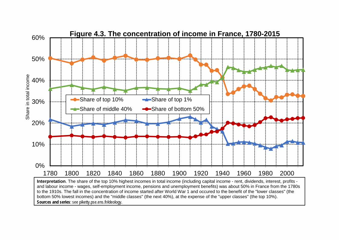
Figure 4.3. The concentration of income in France, 1780-2015
Share of top 10% Share of top 1%
Share of middle 40% Share of bottom 50%
Interpretation. The share of the top 10% highest incomes in total income (including capital income - rent, dividends, interest, profits -and labour income - wages, self-employment income, pensions and unemployment benefits) was about 50% in France from the 1780s to the 1910s. The fall in the concentration of income started after World War 1 and occured to the benefit of the "lower classes" (the bottom 50% lowest incomes) and the "middle classes" (the next 40%), at the expense of the "upper classes" (the top 10%). Sources and series: see piketty.pse.ens.fr/ideology.et
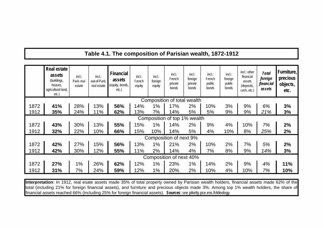
1872 41% 28% 13% 56% 14% 1% 17% 2% 10% 3% 9% 6% 3%1912 35% 24% 11% 62% 13% 7% 14% 5% 5% 9% 9% 21% 3%
1872 43% 30% 13% 55% 15% 1% 14% 2% 9% 4% 10% 7% 2%1912 32% 22% 10% 66% 15% 10% 14% 5% 4% 10% 8% 25% 2%
1872 42% 27% 15% 56% 13% 1% 21% 2% 10% 2% 7% 5% 2%1912 42% 30% 12% 55% 11% 2% 14% 4% 7% 8% 9% 14% 3%
1872 27% 1% 26% 62% 12% 1% 23% 1% 14% 2% 9% 4% 11%1912 31% 7% 24% 59% 12% 1% 20% 2% 10% 4% 10% 7% 10%
Composition of top 1% wealth
Composition of next 9%
Composition of next 40%
Interpretation: In 1912, real esate assets made 35% of total property owned by Parisian wealth holders, financial assets made 62% of thetotal (including 21% for foreign financial assets), and furniture and precious objects made 3%. Among top 1% wealth holders, the share offinancial assets reached 66% (including 25% for foreign financial assets). Sources: see piketty.pse.ens.fr/ideology.
incl.: foreign private bonds
incl.: French public bonds
incl.: foreign public bonds
incl.: other financial assets
(deposits, cash, etc.)
Composition of total wealth
Table 4.1. The composition of Parisian wealth, 1872-1912
Real estate assets (buildings, houses,
agricultural land, etc.)
incl.: Paris real
estate
Furniture, precious objects,
etc.
Financial assets
(equity, bonds, etc.)
incl.: out-of-Paris real estate
incl.: French private bonds
incl.: French equity
Total foreign
financial assets
incl.: foreign equity

0,0%
0,5%
1,0%
1,5%
2,0%
2,5%
3,0%
3,5%
4,0%
4,5%
5,0%
5,5%
1590 1700 1770 1840 1930 1660 1780 1870 1530 1690 1800
Sha
re in
adu
lt m
ale
popu
latio
n
Figure 5.1. The weight of the clergy in Europe, 1530-1930
Interpretation. The clergy made over 4,5% of adult male population in Spain in 1700, less than 3,5% in 1770, and less than 2% in 1840. One observes a general downward trend, but with different chronologies across countries: the fall happens latter in Spain, earlier in Britain, and intermediate in France. Sources and series: see piketty.pse.ens.fr/ideology.012, le candidat de gauche (Hollande) obtient 47% des voix parmi les électeurs sans diplôme (en dehors du certificat d'études primaires), 50% parmi les diplômés du secondaire (Bac, Brevet, Bep, etc.), 53% parmi les diplômés du supérieur court (bac+2) en 2012 le candidat de gauche (Hollande) obtient 47% des voix parmi les électeurs sans diplôme (en dehors du certificat d'études
Spain France Britain

0,0%
1,0%
2,0%
3,0%
4,0%
5,0%
6,0%
7,0%
8,0%
France1660
France1780
Britain1690
Britain1800
Britain1880
Sweden1750
Sweden1850
Spain1750
Portugal1800
Poland1750
Hongary1790
Croatia1790
Sha
re in
tota
l pop
ulat
ion
Figure 5.2. The weight of the nobility in Europe, 1660-1880
Interpretation. The nobility made less than 2% of the population in France, Britain and Sweden during the 17th-19th centuries (with a downward trend), and between 5% and 8% of the population in Spain, Portugal, Poland, Hungary and Croatia. Sources and series: see piketty.pse.ens.fr/ideology.012, le candidat de gauche (Hollande) obtient 47% des voix parmi les électeurs sans diplôme (en dehors du certificat d'études primaires), 50% parmi les diplômés du secondaire (Bac, Brevet, Bep, etc.), 53% parmi les diplômés du supérieur court (bac+2) en 2012, le candidat de gauche (Hollande) obtient 47% des voix parmi les électeurs sans diplôme (en dehors du certificat d'études primaires), 50% parmi les diplômés du secondaire (Bac, Brevet, Bep, etc.), 53% parmi les diplômés du supérieur court (bac+2)

0%
10%
20%
30%
40%
50%
60%
70%
80%
90%
100%
1820 1840 1870 1890 1920 1820 1840 1880 1820 1900 1920
Pro
porti
on o
f adu
lt m
en w
ith th
e rig
ht to
vot
e
Figure 5.3. The evolution of male suffrage in Europe, 1820-1920
Interpretation. The proportion of adult men with the right to vote (taking into account the electoral franchise, i.e. the level of taxes to pay and/or of property to own in order to be granted this right) rose in Britain from 5% in 1820 to 30% in 1870 and 100% in 1920, and in France from 1% in 1820 to 100% in 1880. Sources and series: see piketty.pse.ens.fr/ideology.012, le candidat de gauche (Hollande) obtient 47% des voix parmi les électeurs sans diplôme (en dehors du certificat d'études primaires), 50% parmi les diplômés du secondaire (Bac, Brevet, Bep, etc.), 53% parmi les diplômés du supérieur court (bac+2) en 2012 le candidat de gauche (Hollande) obtient 47% des voix parmi les électeurs sans diplôme (en dehors du
Britain France Sweden

0%
10%
20%
30%
40%
50%
60%
70%
80%
90%
100%
1780 1800 1820 1840 1860 1880 1900 1920 1940 1960 1980 2000
Sha
re in
tota
l priv
ate
prop
erty
Figure 5.4. The concentration of property in Britain, 1780-2015
Share owned by the top 10%
Share owned by the top 1%
Share owned by the middle 40%
Share owned by the bottom 50%
Interpretation. The share owned by the richest 10% in total private property (all assets combined: real estate, business and financial assets, net of debt) was around 85%-92% in Britain between the 1780s and the 1910s. The fall in the concentration of wealth begins after World War 1 and is interrupted in the 1980s. It occurred mostly to the benefit of the "patrimonial middle classes" (the middle 40%), here defined as the intermediate group between the "lower classes" (the bottom 50%) and the the "upper classes" (the top 10%). Sources and series: see piketty.pse.ens.fr/ideologie.et
0%
10%
20%
30%
40%
50%
60%
70%
80%
90%
100%
1780 1800 1820 1840 1860 1880 1900 1920 1940 1960 1980 2000
Sha
re in
tota
l priv
ate
prop
erty
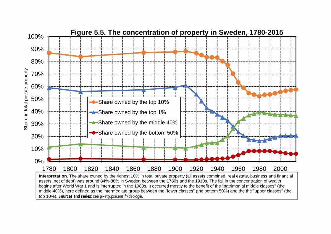
Figure 5.5. The concentration of property in Sweden, 1780-2015
Share owned by the top 10%
Share owned by the top 1%
Share owned by the middle 40%
Share owned by the bottom 50%
Interpretation. The share owned by the richest 10% in total private property (all assets combined: real estate, business and financial assets, net of debt) was around 84%-88% in Sweden between the 1780s and the 1910s. The fall in the concentration of wealth begins after World War 1 and is interrupted in the 1980s. It occurred mostly to the benefit of the "patrimonial middle classes" (the middle 40%), here defined as the intermediate group between the "lower classes" (the bottom 50%) and the the "upper classes" (the top 10%). Sources and series: see piketty.pse.ens.fr/ideologie.et

0%
10%
20%
30%
40%
50%
60%
70%
80%
90%
France Britain Sweden
Sha
re in
tota
l priv
ate
prop
erty
Figure 5.6. Extreme patrimonial inequality: Europe's proprietarian societies during the Belle Epoque (1880-1914)
Bottom 50%
Next 40%
Top 10%
Interpretation. The share the richest 10% in total private property (all assets combined: real estate, business and financial assets, net of debt) was on average 84% in France between 1880 and 1914 (vs. 14% for the next 40% and 2% for the bottom 50%), 91% in Britain (vs 8% and 1%) and 88% in Sweden (vs 11% and 1%). Sources and series: see piketty.pse.ens.fr/ideology.et
Top 10% Top 10%
Next 40%
Next 40% Bottom
50% Bottom 50%

0%
10%
20%
30%
40%
50%
France Britain Sweden
Sha
re in
tota
l nat
iona
l inc
ome
Figure 5.7. Income inequality in Europe's proprietarian societies during the Belle Epoque (1880-1914)
Bottom 50%
Next 40%
Top 10%
Interpretation. The share of the top 10% highest incomes in total national income (labour and capital income) was on average 51% in france between 1880 and 1914 (vs 36% for the next 40% and 13% for the bottom 50%), 55% in Britain (vs 33% and 12%) and 53% in Sweden (vs 34% and 13%). Sources and series: see piketty.pse.ens.fr/ideology.et
Top 10% Top 10%
Next 40%
Next 40%
Bottom 50%
Bottom 50%
0%
10%
20%
30%
40%
50%
60%
70%
80%
90%
South U.S.1800
South U.S.1860
Brasil1750
Brasil1880
Jamaica1830
Barbados1830
Martinique1790
Guadeloupe1790
St Domingue1790
Sha
re o
f sla
ves
in to
tal p
opul
atio
n
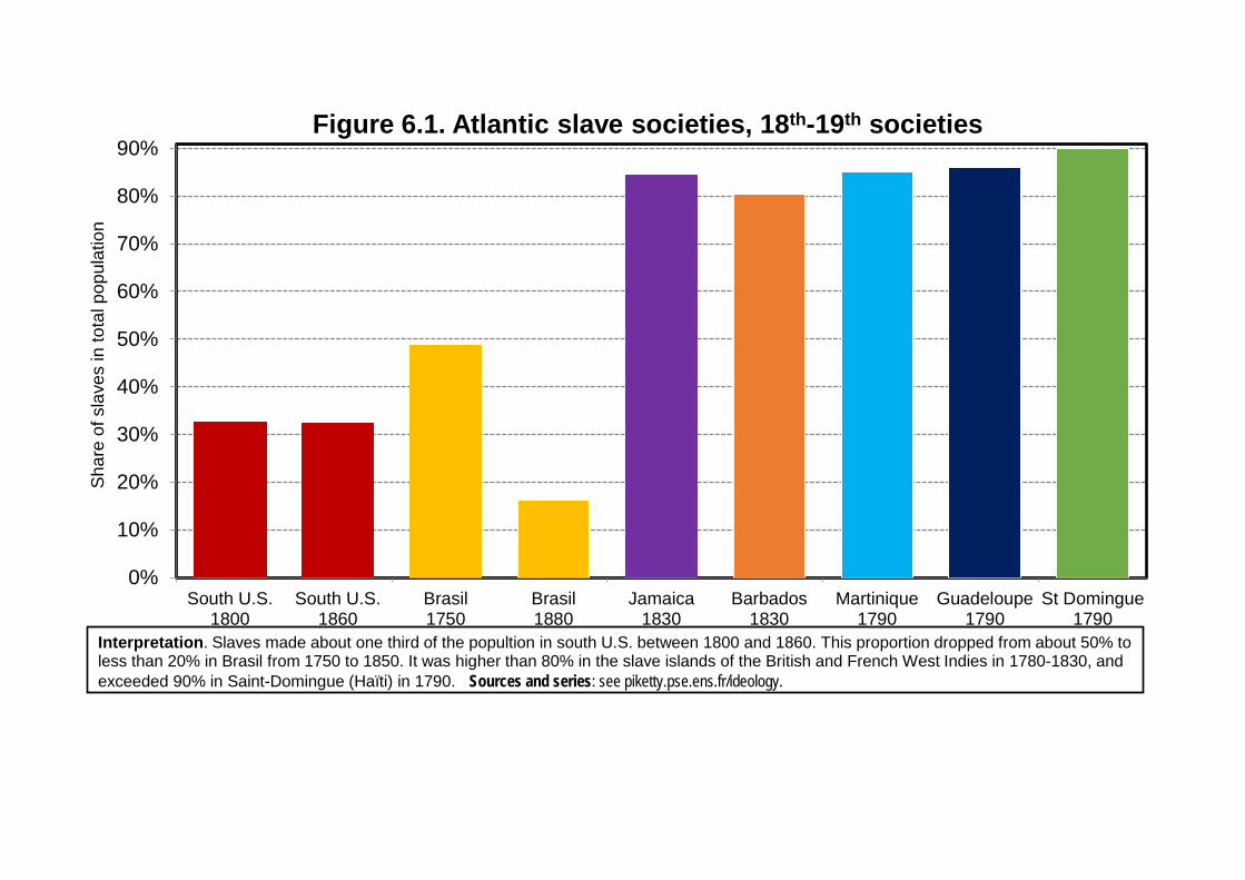
Figure 6.1. Atlantic slave societies, 18th-19th societies
Interpretation. Slaves made about one third of the popultion in south U.S. between 1800 and 1860. This proportion dropped from about 50% toless than 20% in Brasil from 1750 to 1850. It was higher than 80% in the slave islands of the British and French West Indies in 1780-1830, and exceeded 90% in Saint-Domingue (Haïti) in 1790. Sources and series: see piketty.pse.ens.fr/ideology.012, le candidat de gauche (Hollande) obtient 47% des voix parmi les électeurs sans diplôme (en dehors du certificat d'études primaires), 50% parmi les diplômés du secondaire (Bac, Brevet, Bep, etc.), 53% parmi les diplômés du supérieur court (bac+2) en 2012, le candidat de gauche (Hollande) obtient 47% des voix parmi les électeurs sans diplôme (en dehors du certificat d'études primaires), 50% parmi les diplômés du secondaire (Bac, Brevet, Bep, etc.), 53% parmi les diplômés du supérieur court (bac+2) Source: calculs de l'auteur à partir des enquêtes post électorales 1956 2017 (élections présidentielles et législatives)
0
50
100
150
200
250
300
350
400
450
500
550
1700 1710 1720 1730 1740 1750 1760 1770 1780 1790
Pop
ulat
ion
in th
ousa
ds in
habi
tant
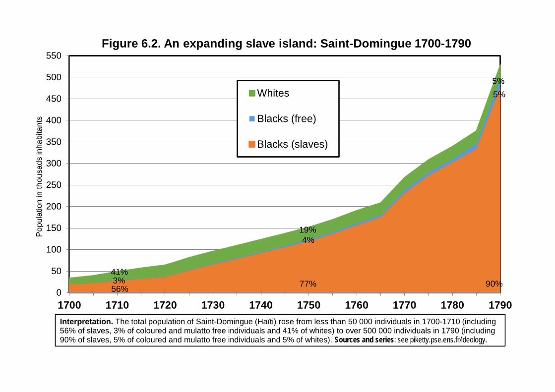
sFigure 6.2. An expanding slave island: Saint-Domingue 1700-1790
Whites
Blacks (free)
Blacks (slaves)
19%
77%
4%
Interpretation. The total population of Saint-Domingue (Haïti) rose from less than 50 000 individuals in 1700-1710 (including 56% of slaves, 3% of coloured and mulatto free individuals and 41% of whites) to over 500 000 individuals in 1790 (including 90% of slaves, 5% of coloured and mulatto free individuals and 5% of whites). Sources and series: see piketty.pse.ens.fr/ideology.
3%41%
56%
5%5%
90%

0%5%
10%15%20%25%30%35%40%45%50%55%60%65%70%
1790 1800 1810 1820 1830 1840 1850 1860
Pro
porti
on o
f sla
ves
in to
tal p
opul
atio
n of
eac
h S
tate
Figure 6.3. The proportion of slaves in the United States 1790-1860South Carolina VirginiaGeorgia North CarolinaKentucky DelawareNew York New Jersey
Interpretation. The proportion of slaves in total population rose or remained stable at a high level in the main southen slave States between 1790 and 1860 (between 35% and 55% in 1850-1860, up to 57%-58% in South Carolina), while slavery dropped or disappeared in Northern States. Sources and series: voir piketty.pse.ens.fr/ideologie.et
0,0
0,5
1,0
1,5
2,0
2,5
3,0
3,5
4,0
4,5
5,0
5,5
6,0
6,5
1700 1750 1780 1820 1860 1880 1890
Num
ber o
f sla
ves
in m
illion
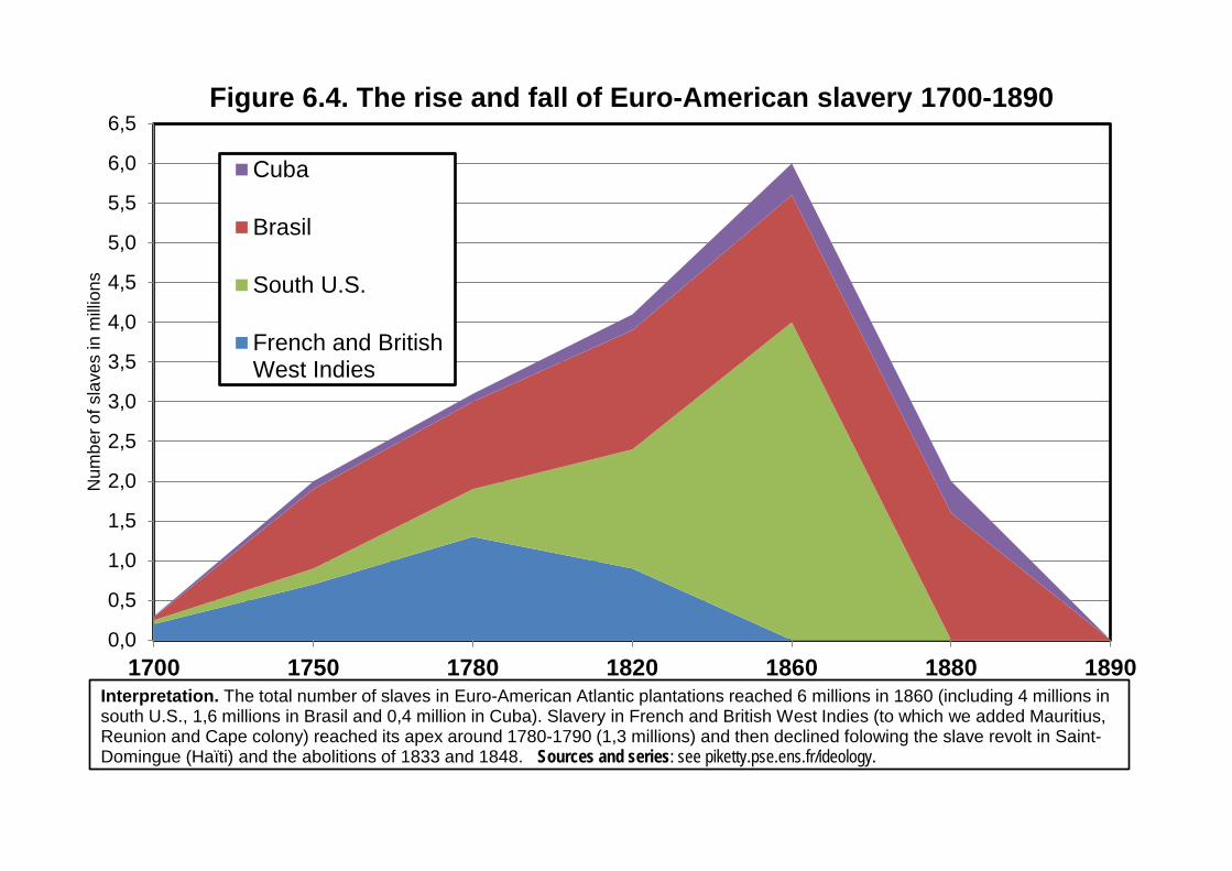
sFigure 6.4. The rise and fall of Euro-American slavery 1700-1890
Cuba
Brasil
South U.S.
French and BritishWest Indies
Interpretation. The total number of slaves in Euro-American Atlantic plantations reached 6 millions in 1860 (including 4 millions in south U.S., 1,6 millions in Brasil and 0,4 million in Cuba). Slavery in French and British West Indies (to which we added Mauritius, Reunion and Cape colony) reached its apex around 1780-1790 (1,3 millions) and then declined folowing the slave revolt in Saint-Domingue (Haïti) and the abolitions of 1833 and 1848. Sources and series: see piketty.pse.ens.fr/ideology.
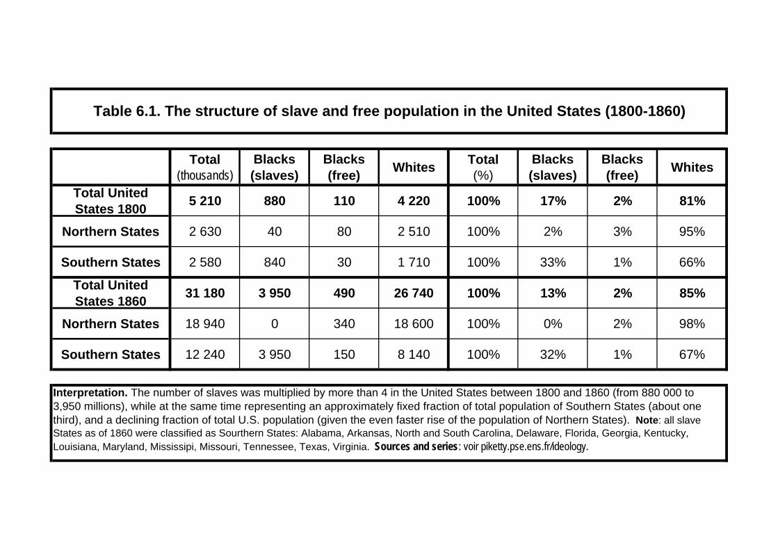
Total (thousands)
Blacks (slaves)
Blacks (free) Whites Total
(%)Blacks (slaves)
Blacks (free) Whites
Total United States 1800 5 210 880 110 4 220 100% 17% 2% 81%
Northern States 2 630 40 80 2 510 100% 2% 3% 95%
Southern States 2 580 840 30 1 710 100% 33% 1% 66%
Total United States 1860 31 180 3 950 490 26 740 100% 13% 2% 85%
Northern States 18 940 0 340 18 600 100% 0% 2% 98%
Southern States 12 240 3 950 150 8 140 100% 32% 1% 67%
Table 6.1. The structure of slave and free population in the United States (1800-1860)
Interpretation. The number of slaves was multiplied by more than 4 in the United States between 1800 and 1860 (from 880 000 to 3,950 millions), while at the same time representing an approximately fixed fraction of total population of Southern States (about one third), and a declining fraction of total U.S. population (given the even faster rise of the population of Northern States). Note: all slave States as of 1860 were classified as Sourthern States: Alabama, Arkansas, North and South Carolina, Delaware, Florida, Georgia, Kentucky, Louisiana, Maryland, Mississipi, Missouri, Tennessee, Texas, Virginia. Sources and series: voir piketty.pse.ens.fr/ideology.

0%1%2%3%4%5%6%7%8%9%
10%11%12%
India1930
Indochina1930
Indonesia1938
Kenya1930
AOF- AEF1950
Madag.1945
Morocco1950
Tunisia1950
Algeria1955
SouthAfrica 2010
Sha
re o
f Eur
opea
ns in
tota
l pop
ulat
ion
Figure 7.1. The weight of Europeans in colonial societies
Interpretation. Between 1930 and 1955, the share of Europeans in colonial societies was 0,1%-0,3% of total population in India, Indochina and Indonesia, 0,3%-0,4% in Kenya, in AOF (Afrique occidentale française, West French Africa) and AEF (Afrique équatoriale française, Equatorial French Africa), 1,2% in Madagascar, 4% in Marocco, 8% in Tunisia, 10% in Algeria (13% in 1906, 14% in 1931). Whites made 11% of South African population in 2010 (it was between 15% and 20% from 1910 to 1990). Sources and series: see piketty.pse.ens.fr/ideology.012, le candidat de gauche (Hollande) obtient 47% des voix parmi les électeurs sans diplôme (en dehors du certificat d'études primaires), 50% parmi les diplômés du secondaire (Bac, Brevet, Bep, etc.), 53% parmi les diplômés du supérieur court (bac+2) en 2012, le candidat de gauche (Hollande) obtient 47% des voix parmi les électeurs sans diplôme (en dehors du certificat d'études primaires), 50% parmi les diplômés du secondaire (Bac, Brevet, Bep, etc.), 53% parmi les

0%
10%
20%
30%
40%
50%
60%
70%
80%
France 1910 Algeria 1930 Haïti 1780
Sha
re in
tota
l nat
iona
l inc
ome
Figure 7.2. Inequality in colonial and slave societies
Bottom 50%
Next 40%
Top 10%
Interpretation. The share of the top 10% highest incomes in total income exceeded 80% in Saint-Domingue (Haïti) in 1780 (then made of about 90% slaves and less than 10% Europeans settlers), vs close to 70% in colonial Algeria in 1930 (then made of about 90% local population and 10% European settlers), and about 50% in metropolitan France in 1910. Sources and series: see piketty.pse.ens.fr/ideology.et
Top 10% Top 10%
Next 40%
Next 40%
Bottom 50%
Bottom 50%

0%
10%
20%
30%
40%
50%
60%
70%
80%
90%
Sweden1980
Europe2018
U.S.2018
Europe1910
Brasil2018
Middle East2018
Algeria1930
South Afr.1950
Haïti1780
Sha
re o
f top
dec
ile in
tota
l inc
ome
Figure 7.3. Extreme income inequality in historical perspective
Interpretation. Over all observed societies, the share of total income received by the top 10% highest incomes varied from 23% in Sweden in 1980 to 81% in Saint-Domingue (Haïti) in 1780 (which included 90% of slaves). Colonial societies such as Algeria and South Africa have in 1930-1950 among the highest inequality levels ever observed in history, with about 70% of total income received by the top decile, which includes approximately the European population. Sources and series: voir piketty.pse.ens.fr/ideology.012, le candidat de gauche (Hollande) obtient 47% des voix parmi les électeurs sans diplôme (en dehors du certificat d'études primaires), 50% parmi les diplômés du secondaire (Bac, Brevet, Bep, etc.), 53% parmi les diplômés du supérieur court (bac+2) en 2012, le candidat de gauche (Hollande) obtient 47% des voix parmi les électeurs sans diplôme (en dehors du certificat d'études primaires), 50% parmi les diplômés du secondaire (Bac, Brevet, Bep,

0%
5%
10%
15%
20%
25%
30%
35%
Sweden1980
Europe2018
U.S.2018
Europe1910
Cameroon1945
Algeria1930
Tanzania1950
Brasil2018
Indochina1935
Mid.East2018
SouthAfrica 1950
Zimbabwe1950
Zambia1950
Sha
re o
f top
per
cent
ile in
tota
l inc
ome
Figure 7.4. The top percentile in historical and colonial perspective
Interpretation. Over the set of all observed societies (with the exception of slave societies), the share of the top percentile (the top 1%highest incomes) in total income varies from 4% in Sweden in 1980 to 36% in Zambia in 1950. Colonial societies are among the most inegalitarian societies observed in history. Sources and series: see piketty.pse.ens.fr/ideology.012, le candidat de gauche (Hollande) obtient 47% des voix parmi les électeurs sans diplôme (en dehors du certificat d'études primaires), 50% parmi les diplômés du secondaire (Bac, Brevet, Bep, etc.), 53% parmi les diplômés du supérieur court (bac+2) en 2012, le candidat de gauche (Hollande) obtient 47% des voix parmi les électeurs sans diplôme (en dehors du certificat d'études primaires), 50% parmi les diplômés du secondaire (Bac, Brevet, Bep, etc.), 53% parmi les diplômés du supérieur court (bac+2)

20%
25%
30%
35%
40%
45%
50%
55%
60%
65%
70%
75%
Algeria1930
Algeria1950
South Afr.1950
South Afr.1990
South Afr.2018
Reunion1960
Reunion1986
Reunion2018
Martinique1986
Martinique2018
France1910
France1945
France2018
Sha
re o
f top
dec
ile in
tota
l nat
iona
l inc
ome
Figure 7.5. Extreme inequality: colonial and post-colonial trajectories
Interpretation. The share of the top decile (the top 10% highest incomes) dropped in Algeria between 1930 and 1950, and in South Africa between 1950 and 2018, while at the same time remaining at one of the highest levels ever observed. In French overseas departements like Reunion or Martinique, income inequality dropped subtantially but remained at higher levels than in metropolitan France.Sources and series: see piketty.pse.ens.fr/ideology.012, le candidat de gauche (Hollande) obtient 47% des voix parmi les électeurs sans diplôme (en dehors du certificat d'études primaires), 50% parmi les diplômés du secondaire (Bac, Brevet, Bep, etc.), 53% parmi les diplômés du supérieur court (bac+2) en 2012, le candidat de gauche (Hollande) obtient 47% des voix parmi les électeurs sans diplôme (en dehors du certificat d'études primaires), 50% parmi les diplômés du secondaire (Bac, Brevet, Bep, etc.), 53% parmi les diplômés du supérieur court (bac+2)

0%
10%
20%
30%
40%
50%
60%
70%
80%
90%
100%
1 1,5 2 2,5 3 4 5 7 10 20 50 100
Max
imal
ineq
ualit
y as
a fu
nctio
n of
ave
rage
inco
me
of a
giv
en
soci
ety
(exp
ress
ed a
s m
ultip
le o
f sub
sist
ence
inco
me)
Figure 7.6. Subsistence income and maximal inequality
Maximal share of top 10% highest incomes(compatible with the subsistence of the poorest)
Maximal share of the top 1% highest incomes
Interpretation. In a society where average income is 3 times larger than subsistence income, the maximal share received by top 10% highest incomes (compatible with a subsistence income for the bottom 90%) is equal to 70% of total income, and the maximal share of top 1% highest incomes (compatible with a substistence income for the bottom 99%) is equal to 67% of total income. The richer the society, the more it is feasible to reach a high inequality level. Sources and series: voir piketty.pse.ens.fr/ideology.et

0%
5%
10%
15%
20%
25%
30%
35%
40%
45%
50%
55%
Sweden1980
Europe2018
U.S.2018
Europe1910
Cameroon1945
Algeria1930
Tanzania1950
Brasil2018
Indochina1935
Mid.East2018
SouthAfrica1950
Zimbabwe1950
Zambia1950
Haïti1780
Sha
re o
f top
per
cent
ile in
tota
l nat
iona
l inc
ome
Figure 7.7. The top percentile in historical perspective (with Haiti)
Interpretation. If we include slave societies like Saint-Domingue (Haïti) in 1780-1790, then the share of income going to the top 1% highest incomes can reach 50%-60% of total income. Sources and series: voir piketty.pse.ens.fr/ideology.012, le candidat de gauche (Hollande) obtient 47% des voix parmi les électeurs sans diplôme (en dehors du certificat d'études primaires), 50% parmi les diplômés du secondaire (Bac, Brevet, Bep, etc.), 53% parmi les diplômés du supérieur court (bac+2) en 2012, le candidat de gauche (Hollande) obtient 47% des voix parmi les électeurs sans diplôme (en dehors du certificat d'études primaires), 50% parmi les diplômés du secondaire (Bac, Brevet, Bep, etc.), 53% parmi les diplômés du

0%
10%
20%
30%
40%
50%
60%
70%
80%
France 1910 France 2018 Algeria 1950
Shar
e of e
duca
tiona
l spe
nding
bene
fiting
the t
op 10
% m
ost fa
vour
ed ch
ildre
n, the
botto
m 50
% le
ast fa
vour
ed, a
nd th
e inte
rmed
iate 4
0%Figure 7.8. Colonies for the colonizers:
the inequality of educational investment in historical perspective
Bottom 50%
Next 40%
Top 10%
Interpretation. In Algeria in 1950, the 10% the most favoured (the settlers) benefited from 82% of total educational spending. By comparison, the share of total educational spending benefiting the top 10% of the population which benefited from the highest educational investement (i.e. those children which did the longest and most expensive studies) was 38% in France in 1930 and 20% in 2018.Sources and series: voir piketty.pse.ens.fr/ideology.et
Top 10%
Top 10%
Next 40%
Next 40%
Bottom 50%
Bottom 50%

-40%
-20%
0%
20%
40%
60%
80%
100%
120%
140%
160%
180%
200%
1810 1830 1850 1870 1890 1910 1930 1950 1970 1990 2010
Fore
ign
asse
ts (n
et o
f lia
bilit
ies)
as
a p
ropo
rtion
of t
he c
ount
ry's
nat
iona
l inc
ime
Figure 7.9. Foreign assets in historical perspective: the French-British colonial apex
Britain FranceGermany JapanUnited States China
Interpretation. Net foreign assets, i.e. the difference between assets owned abroad by resident owners (including in some cases the governement) and liabilities (i.e. assets owned in the country by foreign owners), amounted in 1914 to 191% of national income in Britain and 125% in France. In 2018, net foreign assets reach 80% of national income in Japan, 58% in Germany and 20% in China. Sources and series: see piketty.pse.ens.fr/ideology.et

100
200
400
800
1600
1700 1740 1780 1820 1860 1900 1940 1980 2020 2050
Pop
ulat
ion
in m
illion
s
Figure 8.1. Population in India, China and Europe, 1700-2050
Inde Chine Europe
Interpretation. Around 170, total population was about 170 millions inhabitants in India, 140 millions in China and 100 millions in Eruope (about 125 millions if one includes the territories corresponding to today's Russia, Belarus and Ukraine). In 2050, according to UN projections, total population will be 1,7 billion in India, 1,3 billion in China and 550 millions in Europe (EU+) (720 millions if one includes Russia, Belarus and Ukraine). Sources and series: see piketty.pse.ens.fr/ideology.et

0%
10%
20%
30%
40%
50%
60%
70%
80%
90%
100%
1871 1881 1891 1901 1911 1921 1931 1941 1951 1961 1971 1981 1991 2001 2011
Figure 8.2. The religious structure of India, 1871-2011
Interpretation. in the 2011 census, 80% of India's population was reported as "hindus", 14% as "muslims" and 6% from another religion (sikhs, christians, buddhists, no religion, etc.). These figures were 75%, 20% and 5% in the colonial census of 1871; 72%, 24% and 4% in that of 1941; then 84%, 10% and 6% in the first census conducted by independant India in 1951 (given the partition with Pakistan and Bengladesh). Sources and series: voir piketty.pse.ens.fr/ideology.
20%
5%
75%
6%
14%
80%
Hindus
Muslims
Other religions
72% 84%
10%
6%4%
24%
1871-1941: censuses of British Indian Empire 1951-2011: censuses of independant India

0%
1%
2%
3%
4%
5%
6%
7%
Britain 1530 Britain 1790 France 1560 France 1780 India 1880 India 1930
Sha
re in
adu
lt m
ale
popu
latio
nFigure 8.3. The evolution of ternary societies: Europe-India 1530-1930
Clergy
NobilityNobility
Brahmins
Kshatryas
Interpretation. In Britain and in France, the two dominant classes of the trifunctional society (clergy and nobility) had a declining numerical importance between the 16th and the 18th century. In India, the numerical signficance of brahmins and kshatryas (ancient classes of priests and warriors), as measured by British colonial censuses, dropped slightly between 1880 and 1930, albeit at significantly higher levels than the corresponding classes in Europe in the 16th-18th centuries. Sources and series: see piketty.pse.ens.fr/ideology.012, le candidat de ga che (Hollande) obtient 47% des oi parmi les électe rs sans diplôme (en dehors d certificat d'ét des primaires) 50% parmi les diplômés d
Clergy
ClergyNobility
Nobility
Clergy
Brahmins
Kshatryas
0%1%2%3%4%5%6%7%8%9%
10%11%12%13%14%15%
1870 1890 1910 1930 1950 1970 1990 2010
Sha
re in
tota
l hin
du p
opul
atio
n
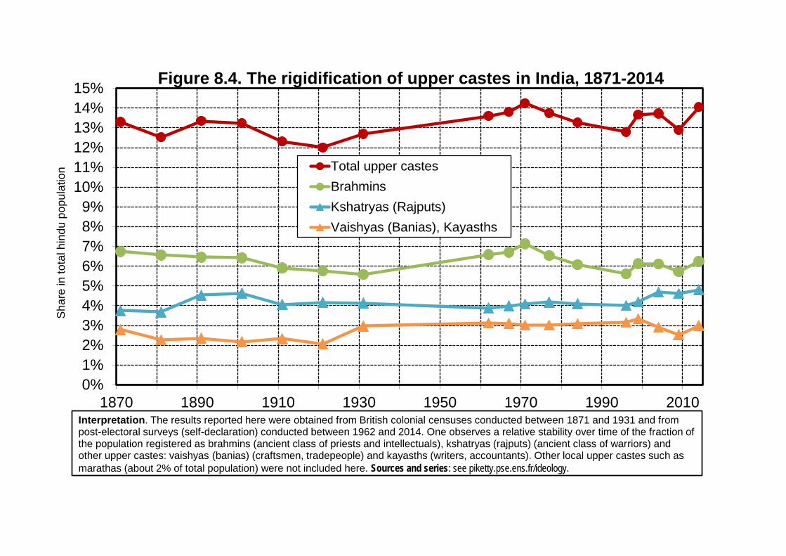
Figure 8.4. The rigidification of upper castes in India, 1871-2014
Total upper castesBrahminsKshatryas (Rajputs)Vaishyas (Banias), Kayasths
Interpretation. The results reported here were obtained from British colonial censuses conducted between 1871 and 1931 and from post-electoral surveys (self-declaration) conducted between 1962 and 2014. One observes a relative stability over time of the fraction of the population registered as brahmins (ancient class of priests and intellectuals), kshatryas (rajputs) (ancient class of warriors) and other upper castes: vaishyas (banias) (craftsmen, tradepeople) and kayasths (writers, accountants). Other local upper castes such as marathas (about 2% of total population) were not included here. Sources and series: see piketty.pse.ens.fr/ideology.et

0%5%
10%15%20%25%30%35%40%45%50%55%60%65%70%75%
1950 1960 1970 1980 1990 2000 2010
Sha
re in
tota
l Ind
ian
popu
latio
n
Figure 8.5. Positive discrimination in India, 1950-2015
Classes benefiting from quotas(OBC + SC + ST)Other backward classes (OBC)
Scheduled castes & tribes (SC + ST)
Schedules castes (SC)
Scheduled tribes (ST)
Interpretation. The results reported here were obtained from the decennial censuses 1951-2011 and NSS surveys 1983-2014. Quotas for accessing universities and public sector jobs were enacted for "scheduled castes" (SC) and "scheduled tribes" (ST) (ancient discriminated groups of untouchables and aborigenal tribes) in 1950, before being gradually extended beginning in 1980-1990 to "other backwardclasses" (OBC) (ancient shudras), following the Mandal commission in 1979-1980. OBCs are registered in NSS surveys since 1999 only, so the estimates reported here for 1981 and 1991 (35% of population) are approximate. Sources and series: see piketty.pse.ens.fr/ideology.et

0%
10%
20%
30%
40%
50%
60%
70%
80%
1950 1960 1970 1980 1990 2000 2010
Figure 8.6. Discrimination and inequality in comparative perspective
India: average income lower castes (SC+ST)/rest of the population
United States: average income blacks/whites
South Africa: average income blacks/whites
Interpretation. The ratio between the average income of lower castes in India (scheduled castes and tribes, SC+ST, ancient discriminated groups of untouchables and aborigenal tribes) and that of the rest of the population rise from 57% in 1950 to 74% in 2014. The ratio between the average income of Blacks and Whites rose over the same period from 54% to 56% in the United States, and from 9% to 18% in South Africa. Sources et séries: see piketty.pse.ens.fr/ideology.et

1871 1881 1891 1901 1911 1921 1931 1941 1951 1961 1971 1981 1991 2001 2011
Hindus 75% 76% 76% 74% 73% 72% 71% 72% 84% 83% 83% 82% 81% 81% 80%
Muslims 20% 20% 20% 21% 21% 22% 22% 24% 10% 11% 11% 12% 13% 13% 14%
Other religions (sikhs, christians, buddhists, etc.) 5% 4% 4% 5% 6% 6% 7% 4% 6% 6% 6% 6% 6% 6% 6%
Total 100% 100% 100% 100% 100% 100% 100% 100% 100% 100% 100% 100% 100% 100% 100%
Scheduled castes (SC) 15% 15% 15% 16% 17% 16% 17%
Schedules tribes (ST) 6% 7% 7% 8% 8% 8% 9%
Total Indian population (millions) 239 254 287 294 314 316 351 387 361 439 548 683 846 1 029 1 211
Table 8.1. The structure of the population in censuses of India, 1871-2011
Interpretation: The results reported here were obtained using the decennial censuses conducted in British colonial India between 1871 and 1941 and in independant India from 1951 to 2011. The proportion of Muslims falls from 24% in 1941 to 10% in 1951, due to the partition with Pakistan. Starting in 1951, censuses register "scheduled castes" (SC) and "scheduled tribes" (ST) (untouchables and aborigenal tribes formerly discriminated), which can belong to the various religions (mostly hindus and other religions). Sources and series: see piketty.pse.ens.fr/ideology.

1871 1881 1891 1901 1911 1921 1931 1962 1967 1971 1977 1996 1999 2004 2009 2014
Total upper castes 13,3% 12,6% 13,4% 13,2% 12,3% 12,0% 12,7% 13,6% 13,8% 14,2% 13,7% 12,8% 13,6% 13,7% 12,8% 14,0%
incl. Brahmins (priests, intellectuals) 6,7% 6,6% 6,5% 6,4% 5,9% 5,8% 5,6% 6,6% 6,7% 7,1% 6,5% 5,6% 6,1% 6,1% 5,7% 6,2%
incl. Kshatryas (Rajputs) (warriors) 3,8% 3,7% 4,5% 4,6% 4,1% 4,2% 4,1% 3,9% 4,0% 4,1% 4,2% 4,0% 4,2% 4,7% 4,6% 4,8%
incl. other upper castes: Vaishyas
(Banias), Kayasths2,8% 2,3% 2,4% 2,2% 2,3% 2,1% 3,0% 3,1% 3,1% 3,0% 3,0% 3,2% 3,3% 2,9% 2,5% 3,0%
Total hindu population (millions)
179 194 217 217 228 226 247 375 419 453 519 759 800 870 939 1 012
Table 8.2. The structure of upper castes in India, 1871-2014
Interpretation: The results reported here were obtained using the British colonial censuses of India conducted between 1871 and 1931 and the post-electoral surveys (self-declaration) run from 1962 to 2014. One observes a relative stability of the proportion of the population registered as brahmins (former classes of priests and intellectuals), kshatryas (rajputs) (former classes of warriors) and other upper castes: vaishyas (banias) (craftsmen, tradespeople) and kayasths (writers, accountants). Other local upper castes such as the marathas (about 2% of population) were not included here. Sources and series: see piketty.pse.ens.fr/ideology.

0
200
400
600
800
1000
1200
1400
1600
1800
2000
1500 1550 1600 1650 1700 1750 1800
Fisc
al re
venu
es in
equ
ival
ent t
ons
of s
ilver
Figure 9.1. The fiscal capacity of States, 1500-1780 (tons of silver)
France
England
Spain-Holland
Austria-Prussia
Ottoman Empire
Interpretation. Around 1500-1550, the fiscal revenues of the main European States and of the Ottoman Empire were at a level equivalent to about 100-200 silver tons per year. In the 1780s, the fiscal revenus of France and England were between 1600 and 2000 tons of sliver per year, while those of the Ottoman Empire were less than 200 tons. Sources and series: see piketty.pse.ens.fr/ideology.et

0
2
4
6
8
10
12
14
16
18
20
22
1500 1550 1600 1650 1700 1750 1800 1850
Fisc
al re
venu
es p
er in
habi
tant
in e
quiv
alen
t day
s of
wag
esFigure 9.2. The fiscal capacity of States, 1500-1850 (days of wages)
England
France
Prussia
Ottoman Empire
Chinese Empire
Interpretation. Around 1500-1600, the fiscal revenues par inhabitants of the main European States were between 2 and 4 days of urban unskilled maneuver wages; in 1750-1780, they were between 10 and 20 days of unskilled wages. Per inhabitant fiscal revenues remained around 2-5 days of wages in the Ottoman Empire as well as in the Chinese Empire. With a per inhabitant national income estimated to be around 250 days of unskilled urban wage, this implies that tax revenues have stagnated around 1%-2% of national incime in Chinese and Ottoman Empires, while they rose from 1%-2% to 6%-8% of national income in Europe. Sources and series: see piketty.pse.ens.fr/ideology.et
0%
1%
2%
3%
4%
5%
6%
7%
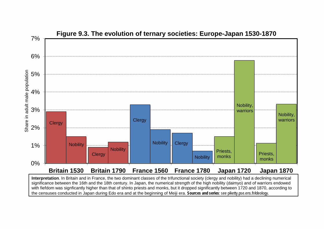
Britain 1530 Britain 1790 France 1560 France 1780 Japan 1720 Japan 1870
Sha
re in
adu
lt m
ale
popu
latio
n
Figure 9.3. The evolution of ternary societies: Europe-Japan 1530-1870
Clergy
NobilityNobility Priests,
monks
Nobility,warriors
Interpretation. In Britain and in France, the two dominant classes of the trifunctional society (clergy and nobility) had a declining numerical significance between the 16th and the 18th century. In Japan, the numerical strength of the high nobility (daimyo) and of warriors endowed with fiefdom was signficantly higher than that of shinto priests and monks, but it dropped significantly between 1720 and 1870, according to the censuses conducted in Japan during Edo era and at the beginning of Meiji era. Sources and series: see piketty.pse.ens.fr/ideology.012, le candidat de gauche (Hollande) obtient 47% des voix parmi les électeurs sans diplôme (en dehors du certificat d'études primaires) 50% parmi les
Clergy
ClergyNobility
Nobility
Clergy
Priests,monks
Nobility,warriors

25%
30%
35%
40%
45%
50%
1900 1910 1920 1930 1940 1950 1960 1970 1980 1990 2000 2010
Sha
re o
f top
dec
ile in
tota
l nat
iona
l inc
ome
Figure 10.1. Income inequality: Europe and the U.S. 1900-2015
United States
Europe
Interpretation. The share of the top decile (the top 10% highest incomes) in total national income was on average about 50% in Western Europe in 1900-1910, before dropping to about 30% in 1950-1980, and rising again above 35% by 2010-2015. The rebound of inequality was much strong in the U.S., where the top decile income share is about 45%-50% in 2010-2015 and exceeds the level observed in 1900-1910. Sources and series: see piketty.pse.ens.fr/ideology.et

20%
25%
30%
35%
40%
45%
50%
1900 1910 1920 1930 1940 1950 1960 1970 1980 1990 2000 2010
Sha
re o
f top
dec
ile in
tota
l nat
iona
l inc
ome
Figure 10.2. Income inequality 1900-2015: the diversity of Europe
United States Europe
Britain France
Sweden Germany
Interpretation. The share of the top decile (the top 10% highest incomes) in total national income was on average about 50% in Western Europe in 1900-1910, before dropping to about 30% in 1950-1980 (or even below 25% in Sweden), and rising again above 35% by 2010-2015 (or even above 40% in Britain). In 2015, Britain and Germany appear to be above European average, while France and Sweden are below average. Sources and series: see piketty.pse.ens.fr/ideology.et

0%
5%
10%
15%
20%
25%
1900 1910 1920 1930 1940 1950 1960 1970 1980 1990 2000 2010
Sha
re o
f top
per
cent
ile in
tota
l nat
iona
l inc
ome
Figure 10.3. Income inequality: the top percentile, 1900-2015
United States Europe
Britain France
Sweden Germany
Interpretation. The share of the top percentile (the 1% highest incomes) in total national income was about 20%-25% in Western Europe in 1900-1910, before dropping to 5%-10% in 1950-1980 (or even less than 5% in Sweden), and rising again around 10%-15% in2010-2015. The rebound of inequality was much stronger in the U.S., where the top percentile share reaches 20% in 2010-2015 and exceeds the level of 1900-1910. Sources and series: see piketty.pse.ens.fr/ideology.et

45%
50%
55%
60%
65%
70%
75%
80%
85%
90%
95%
1900 1910 1920 1930 1940 1950 1960 1970 1980 1990 2000 2010
Sha
re o
f top
dec
ile in
tota
l priv
ate
prop
erty
Figure 10.4. Wealth inequality: Europe & the U.S. 1900-2015
United StatesEuropeBritainFranceSweden
Interpretation. The share of the top decile (the 10% highest wealth holders) in total private property (all assets combined: real estate, business and financial assets, net of debt) was about 90% in Western Europe in 1900-1910, before dropping to 50%-55% in 1980-1990, and rising since then. The rebound of inequality was much stronger in the United States, where the top decile share is close to 75% in 2010-2015 and resembles the level of 1900-1910 . Sources and series: see piketty.pse.ens.fr/ideology.
10%15%20%25%30%35%40%45%50%55%60%65%70%75%
1900 1910 1920 1930 1940 1950 1960 1970 1980 1990 2000 2010
Sha
re o
f top
per
cent
ile in
tota
l priv
ate
prop
erty
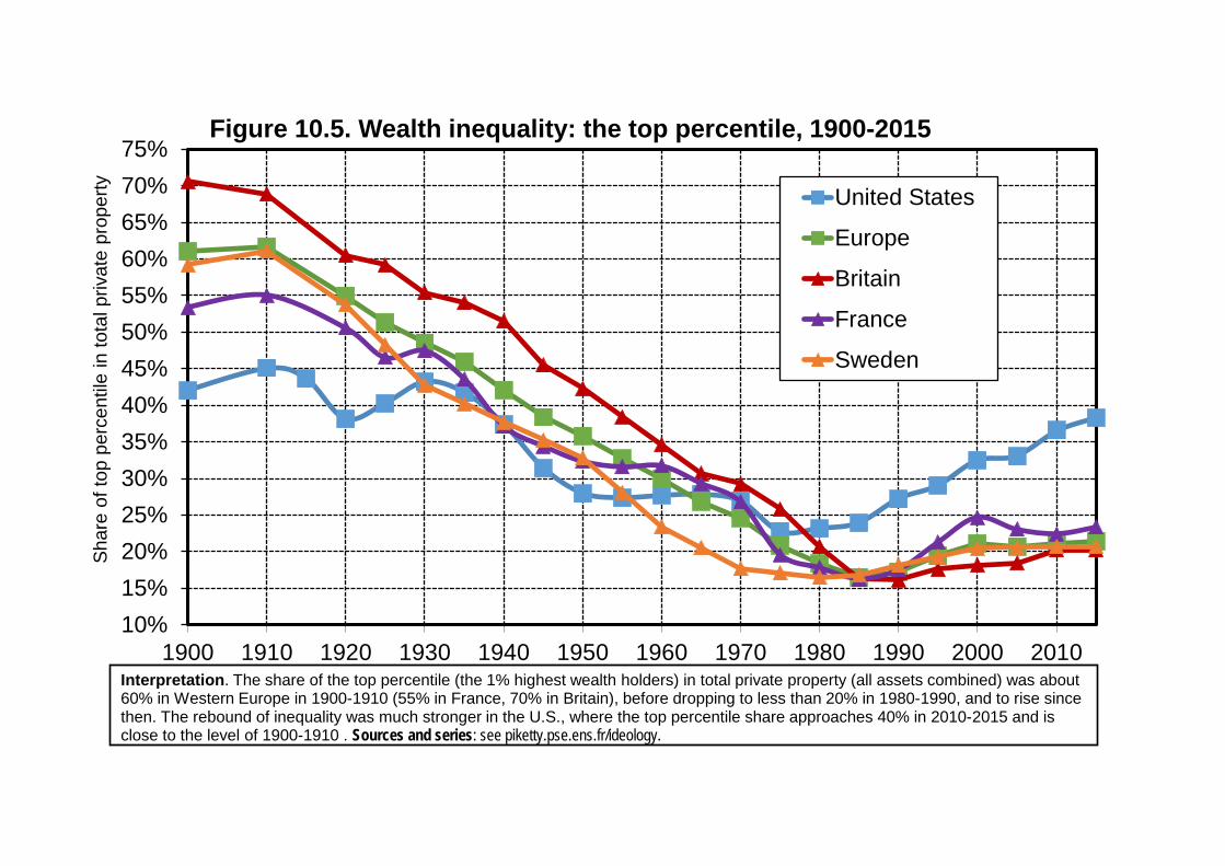
Figure 10.5. Wealth inequality: the top percentile, 1900-2015
United States
Europe
Britain
France
Sweden
Interpretation. The share of the top percentile (the 1% highest wealth holders) in total private property (all assets combined) was about 60% in Western Europe in 1900-1910 (55% in France, 70% in Britain), before dropping to less than 20% in 1980-1990, and to rise since then. The rebound of inequality was much stronger in the U.S., where the top percentile share approaches 40% in 2010-2015 and isclose to the level of 1900-1910 . Sources and series: see piketty.pse.ens.fr/ideology.et

20%25%30%35%40%45%50%55%60%65%70%75%80%85%90%95%
100%
1900 1910 1920 1930 1940 1950 1960 1970 1980 1990 2000 2010
Sha
re o
f top
dec
ile in
cor
resp
ondi
ng to
tal
Figure 10.6. Income vs Wealth Inequality, France 1900-2015Incomes from capitalOwnership of capitalTotal income (capital and labour)Incomes from labour
Interpretation. In 1900-1910, the 10% highest capital incomes (rent, profit, dividend, interest, etc.) received about 90%-95% of total capital incomes; the 10% highest labour incomes (wages, self-employment income, pensions) received about 25%-30% of total labourincomes. The reduction of inequalities during the 20th century came entirely from the fall in the concentration of property, while the inequality of labour incomes changed little. Sources and series: see piketty.pse.ens.fr/ideology.et

0%5%
10%15%20%25%30%35%40%45%50%55%60%65%
1900 1910 1920 1930 1940 1950 1960 1970 1980 1990 2000 2010
Sha
re o
f top
per
cent
ile in
cor
resp
ondi
ng to
tal
Figure 10.7. The top percentile: income vs wealth, France 1900-2015
Income from capitalOwnership of capitalTotal income (labour and capital)Income from labour
Interpretation. In 1900-1910, the 1% highest capital incomes (rent, profit, dividend, interest, etc.) received about 60% of total capital incomes; the 1% highest capital owners (real estate, business and financial assets, net of debt) owned about 55% of total private property; the 1% highest total incomes (labour and capital) received about 20%-25% of total income; the 1% highest labour incomes (wages, self-employment income, pensions) received about 5M-10% of total labour incomes. In the long-run, the fall of inequality is entirely due to the fall in the concentration of property and incomes from capital. Sources and series: see piketty.pse.ens.fr/ideology.et

150%200%250%300%350%400%450%500%550%600%650%700%750%800%
1870 1880 1890 1900 1910 1920 1930 1940 1950 1960 1970 1980 1990 2000 2010
Tota
l priv
ate
asse
ts (n
et o
f deb
t) as
% o
f nat
iona
l inc
ome
Figure 10.8. Private property in Europe, 1870-2020
Britain
France
Germany
Interpretation. The market value of private property (all assets combined: real estate, business and financial assets, net of debt) was about 6-8 years of national income in Western Europe in 1870-1914, before falling from 1914 to 1950 and reaching about 2-3 years of national income in 1950-1970, and then rising again around 5-6 years in 2000-2020. Sources and series: see piketty.pse.ens.fr/ideology.et

0%
50%
100%
150%
200%
250%
300%
1850 1870 1890 1910 1930 1950 1970 1990 2010
Pub
lic d
ebt a
s %
of n
atio
nal i
ncom
eFigure 10.9. The vicissitudes of public debt, 1850-2020
Britain
France
Germany
United States
Interpretation. Public debt rose strongly after each world war and reached between 1500% and 300% of national income in 1945-1950, before falling sharply in Germany and France (debt cancellations, high inflation) and more gradually in Britain and the U.S. (moderate inflation, growth). Public assets (especially real estate and financial assets) have fluctuated less strongly over time and generally represent around 100% of national income. Sources and series: see piketty.pse.ens.fr/ideology.et

-2%
0%
2%
4%
6%
8%
10%
12%
14%
16%
18%
20%
1700-1820 1820-1870 1870-1914 1914-1950 1950-1970 1970-1990 1990-2020
Annu
al in
flatio
n ra
te (c
onsu
mer
pric
e in
dex)
Figure 10.10. Inflation in Europe and the U.S., 1700-2020
Germany
France
Britain
United States
Interpretation. Inflation was quasi-null in the 18th-19th centuries, before rising in the 20th century. It is about 2% per year since 1990. Inflation was particularly high in Germany and France between 1914 and 1950, and to a lesser extent in Britain, France and the U.S. during the 1970s. Note. German inflation reached 17% per year between 1914 and 1950 without taking into account the hyper-inflation of 1923. Sources and series: see piketty.pse.ens.fr/ideology.et
0%
10%
20%
30%
40%
50%
60%
70%
80%
90%
100%
1900 1910 1920 1930 1940 1950 1960 1970 1980 1990 2000 2010 2020
Top
mar
gina
l tax
rate
app
lied
to th
e hi
ghes
t inc
omes
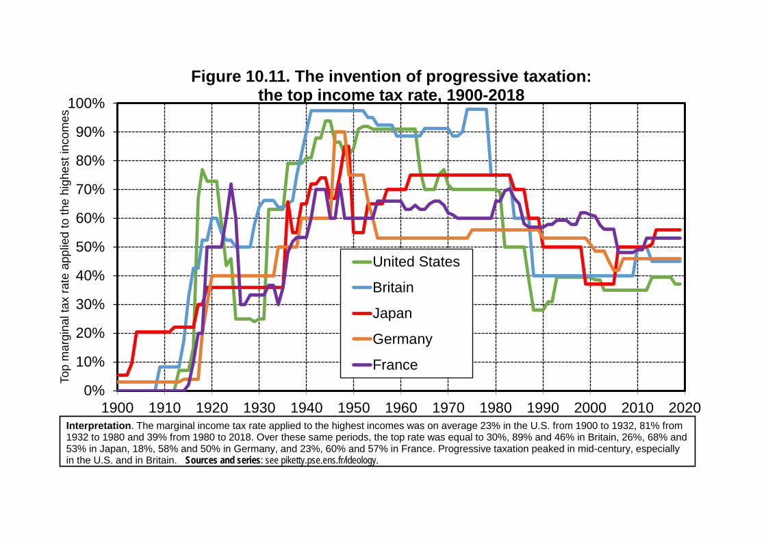
Figure 10.11. The invention of progressive taxation: the top income tax rate, 1900-2018
United States
Britain
Japan
Germany
France
Interpretation. The marginal income tax rate applied to the highest incomes was on average 23% in the U.S. from 1900 to 1932, 81% from 1932 to 1980 and 39% from 1980 to 2018. Over these same periods, the top rate was equal to 30%, 89% and 46% in Britain, 26%, 68% and 53% in Japan, 18%, 58% and 50% in Germany, and 23%, 60% and 57% in France. Progressive taxation peaked in mid-century, especially in the U.S. and in Britain. Sources and series: see piketty.pse.ens.fr/ideology.et
0%
10%
20%
30%
40%
50%
60%
70%
80%
90%
100%
1900 1910 1920 1930 1940 1950 1960 1970 1980 1990 2000 2010 2020
Top
mar
gina
l tax
rate
app
lied
to th
e hi
ghes
t inh
erita
nces
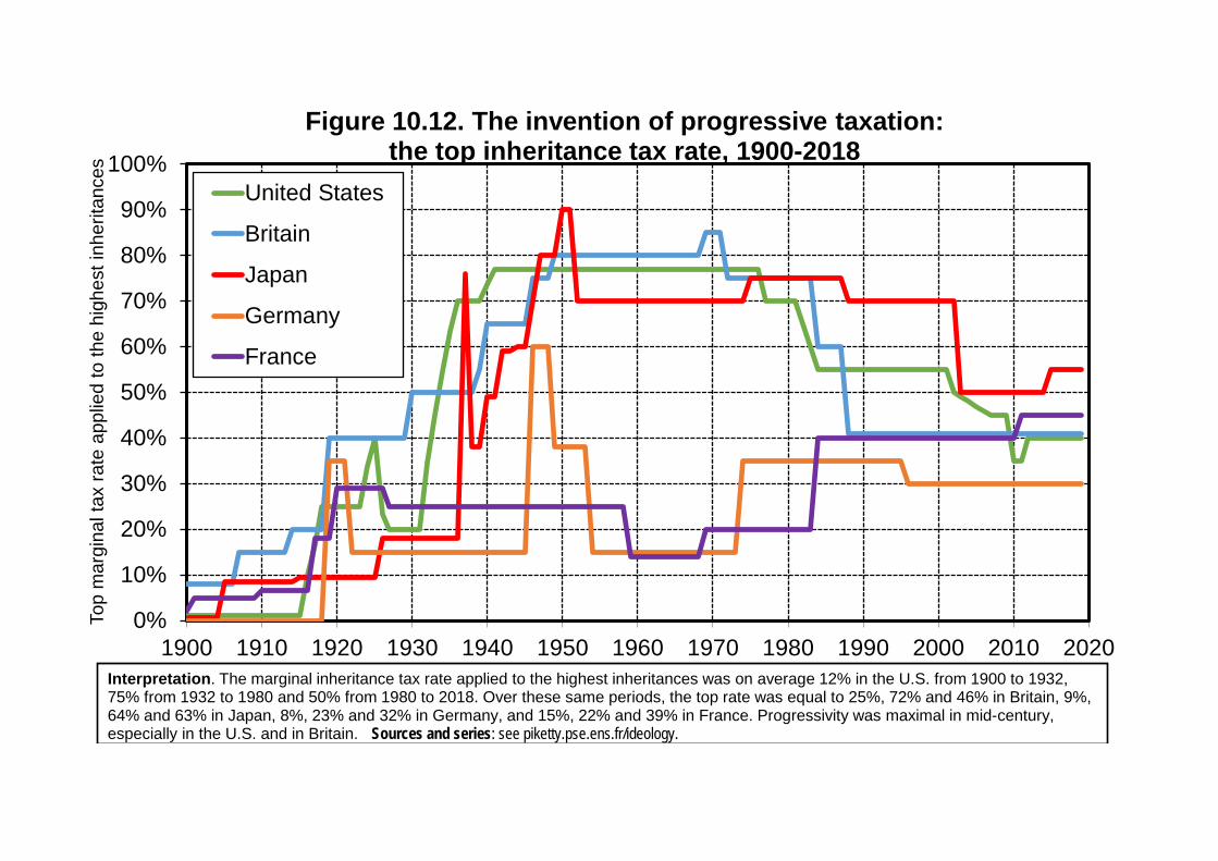
Figure 10.12. The invention of progressive taxation: the top inheritance tax rate, 1900-2018
United States
Britain
Japan
Germany
France
Interpretation. The marginal inheritance tax rate applied to the highest inheritances was on average 12% in the U.S. from 1900 to 1932, 75% from 1932 to 1980 and 50% from 1980 to 2018. Over these same periods, the top rate was equal to 25%, 72% and 46% in Britain, 9%, 64% and 63% in Japan, 8%, 23% and 32% in Germany, and 15%, 22% and 39% in France. Progressivity was maximal in mid-century, especially in the U.S. and in Britain. Sources and series: see piketty.pse.ens.fr/ideology.et

0%
10%
20%
30%
40%
50%
60%
70%
80%
1910 1920 1930 1940 1950 1960 1970 1980 1990 2000 2010 2020
Effe
ctiv
e ta
x ra
tes
(all
taxe
s) a
s %
inco
me
Figure 10.13. Effective rates and progressivity in the U.S. 1910-2020Top 0,01% incomesTop 0,1% incomesTop 1% incomesAverage for total populationBottom 50% incomes
Interpretation. From 1915 to 1980, the tax system was highly progressive in the U.S., in the sense that effective tax rates paid by the highest income groups (all taxes included, and as % of pretax income) was significantly larger than the average effective tax rate paid by the the total population (and particularly by the bottom 50% incomes). Since 1980, the tax system has not been very progressive, with little differences in effective tax rates across groups. Sources and series: see piketty.pse.ens.fr/ideology.et

0%
10%
20%
30%
40%
50%
60%
1870 1880 1890 1900 1910 1920 1930 1940 1950 1960 1970 1980 1990 2000 2010
Tota
l tax
reve
nues
as
% n
atio
nal i
ncom
e
Figure 10.14. The rise of the fiscal State in rich countries 1870-2015
Sweden
France
Germany
Britain
United States
Interpretation. Total fiscal revenues (all taxes and social contributions included) made less than 10% of national income in rich countriesduring the 19th century and until World War 1, before rising strongly from the 1910s-1920s until the 1970s-1980s and then stabilizing at different levels across countries: around 30% in the U.S., 40% in Britain and 45%-55% in Germany, France and Sweden. Sources and series: see piketty.pse.ens.fr/ideology.et

0%
10%
20%
30%
40%
50%
60%
1870 1880 1890 1900 1910 1920 1930 1940 1950 1960 1970 1980 1990 2000 2010
Use
s of
fisc
al re
venu
es a
s %
nat
iona
l inc
ome
Figure 10.15. The rise of the social State in Europe, 1870-2015
Other social spendingSocial transfers (family, unemployment, etc.)Health (health insurance, hospitals, etc.)Retirement and disability pensionsEducation (primary, secondary, tertiary)Army, police, justice, administration, etc.
6%
10%
11%
Interpretation. In 2015, fiscal revenues represented 47% of national income on average in Western Europe et were used as follows: 10% of national income for regalian expenditure (army, police, justice, general administration, basic infrastructure: roads, etc.); 6% for education; 11% for pensions; 9% for health; 5% for social transfers (other than pensions); 6% for other social spending (housing, etc.). Before 1914, regalian expenditure absorbed almost all fiscal revenues. Note. The evolution depicted here is the average of Germany, France, Britain and Sweden (see figure 10.14). Sources and séries: see piketty.pse.ens.fr/ideology.
9%
8%
6%
5%
2%
6%
1%
47%

10
20
40
80
1700 1740 1780 1820 1860 1900 1940 1980 2020 2060 2100
Pop
ulat
ion
in m
illion
s in
habi
tant
s (c
urre
nt te
rrito
ries)
Figure 10.16. Demography and the balance of power in Europe
Germany
France
Britain
Italy
Interpretation. Germany, Britain, Italy and France have had for centuries populations of comparable size: the four countries all had about 20-30 millions inhabitants in 1820, and they all have around 60-80 millions inhabitants in 2020. There have been frequent changes in relative position, however. E.g. in 1800 France was half more numerous than Germany (31 millions vs 22 millions); in 1910, Germany was half more numerous than France (63 millions vs 41 millions). According to UN projections, Britain and France will be the most numerous by 2100. Sources and series: see piketty.pse.ens.fr/ideology.et
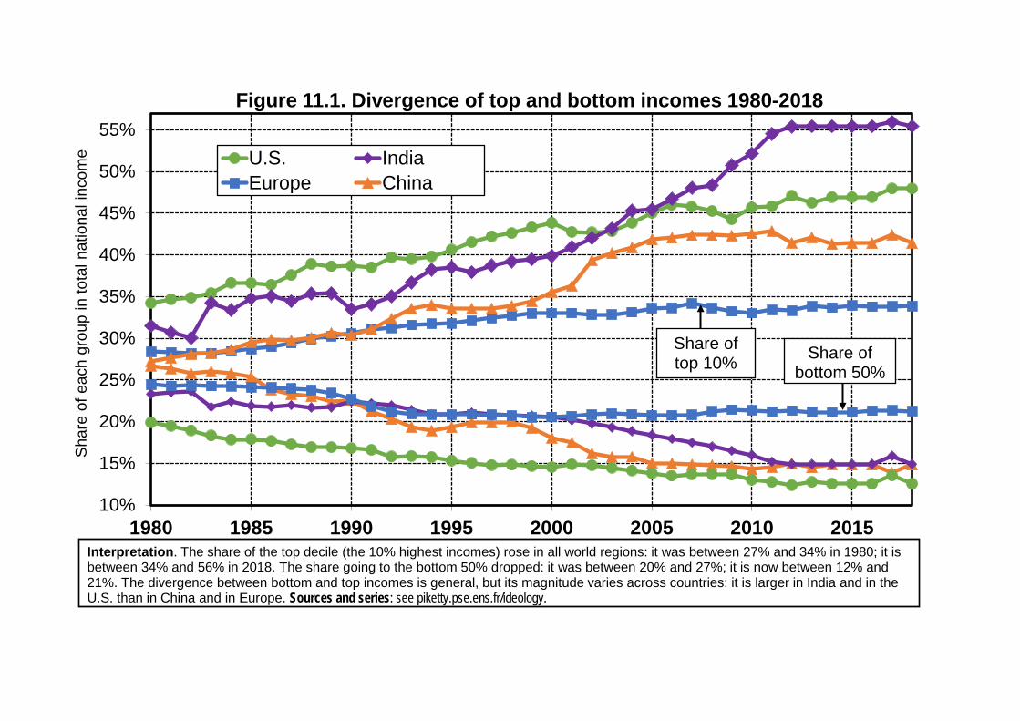
10%
15%
20%
25%
30%
35%
40%
45%
50%
55%
1980 1985 1990 1995 2000 2005 2010 2015
Sha
re o
f eac
h gr
oup
in to
tal n
atio
nal i
ncom
eFigure 11.1. Divergence of top and bottom incomes 1980-2018
U.S. IndiaEurope China
Interpretation. The share of the top decile (the 10% highest incomes) rose in all world regions: it was between 27% and 34% in 1980; it is between 34% and 56% in 2018. The share going to the bottom 50% dropped: it was between 20% and 27%; it is now between 12% and21%. The divergence between bottom and top incomes is general, but its magnitude varies across countries: it is larger in India and in the U.S. than in China and in Europe. Sources and series: see piketty.pse.ens.fr/ideology.et
Share of top 10% Share of
bottom 50%

10%
15%
20%
25%
30%
35%
40%
45%
50%
55%
1900 1910 1920 1930 1940 1950 1960 1970 1980 1990 2000 2010
Sha
re o
f eac
h gr
oup
in n
atio
nal i
ncom
eFigure 11.2. Bottom and top incomes: France & the U.S. 1910-2015
Top 10% share (U.S.)Top 10% share (France)Bottom 50% share (U.S.)Bottom 50% share (France)
248 810 €
112 930 €
13 280€
15 530 €
Interpretation. Income inequality in the U.S. in 2010-2015 exceeded its level in 1900-1910, whereas it was reduced in France (and Europe). In both cases, however, inequality remains high: the top decile, one-fifth the size of the bottom 50 percent, still receives a much larger income share. The income levels reported here are the average annual incomes of each group in 2015 (at purchasing power parity). Sources and series: see piketty.pse.ens.fr/ideology.et

5 €
15 €
25 €
35 €
45 €
55 €
1950 1955 1960 1965 1970 1975 1980 1985 1990 1995 2000 2005 2010 2015
GD
P pe
r hou
r of w
ork
in p
urch
asin
g po
wer
par
ity (€
2015
)Figure 11.3. Labour productivity, 1950-2015 (euros 2015)
United States
Germany
France
Britain
Interpretation. Labour productivity, measured by GDP per hour of work (in euros 2015 and at purchasing power parity) rose from 8 euros in Germany and in France in 1950 to 55 euros in 2015. Germany and France caught up (or slightly passed) the U.S. in 1985-1990, while Britain remains about 20% lower. Sources and series: see piketty.pse.ens.fr/ideology.et

40
45
50
55
60
65
70
75
80
85
90
95
100
105
110
1950 1955 1960 1965 1970 1975 1980 1985 1990 1995 2000 2005 2010 2015
GDP
per h
our o
f wor
k in p
urch
asing
pow
er p
arity
(U.S
. = 10
0)Figure 11.4. Labour productivity : Europe vs United States
United States
Germany
France
Britain
Interpretation. Labour productivity, measured by GDP per hour of work (in euros 2015 and at purchasing power parity), was twice as small in Europe than in the United States in 1950. Germany and France caught up (or slightly passed) the U.S. in 1985-1990, while Britain remains 20% lower. Sources and series: see piketty.pse.ens.fr/ideology.et
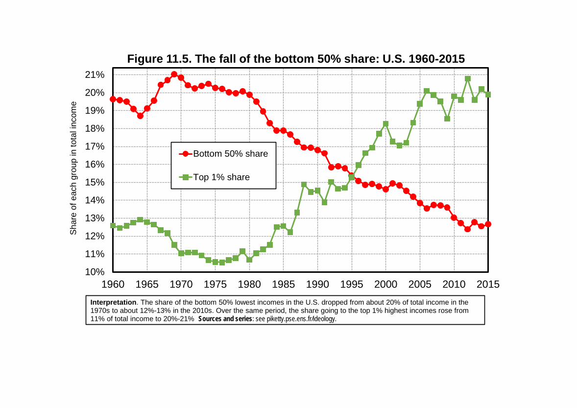
10%
11%
12%
13%
14%
15%
16%
17%
18%
19%
20%
21%
1960 1965 1970 1975 1980 1985 1990 1995 2000 2005 2010 2015
Sha
re o
f eac
h gr
oup
in to
tal i
ncom
eFigure 11.5. The fall of the bottom 50% share: U.S. 1960-2015
Bottom 50% share
Top 1% share
Interpretation. The share of the bottom 50% lowest incomes in the U.S. dropped from about 20% of total income in the 1970s to about 12%-13% in the 2010s. Over the same period, the share going to the top 1% highest incomes rose from 11% of total income to 20%-21% Sources and series: see piketty.pse.ens.fr/ideology.et

6%
8%
10%
12%
14%
16%
18%
20%
22%
24%
26%
1980 1985 1990 1995 2000 2005 2010 2015
Sha
re o
f eac
h gr
oup
in to
tal i
ncom
eFigure 11.6. Low and high incomes in Europe, 1980-2016
Bottom 50% share
Top 1% share
Interpretation. The share of the bottom 50% lowest incomes in Europe dropped from about 26% of total income in the early 1980s to 23% in the 2010s. Over the same period, the share going to the top 1% highest incomes rose from 7% of total income to 10% Sources and series: see piketty.pse.ens.fr/ideology.et

$10 000
$15 000
$20 000
$25 000
$30 000
$35 000
$40 000
$45 000
$300 000
$450 000
$600 000
$750 000
$900 000
$1 050 000
$1 200 000
$1 350 000
1960 1965 1970 1975 1980 1985 1990 1995 2000 2005 2010 2015
Figure 11.7. Low and high incomes in the U.S. 1960-2015
Average income of the top 1%(left axis)
Average income of the bottom 50%(right axis)
Interpretation. In 1970, the average income of the bottom 50% was 15 200$ per year and per adult, and that of the top 1% was 403 000$, i.e. a ratio of 1 to 26. In 2015, the average income of the bottom 50% was 16 200$ and that of the top 1% was 1 305 000$, i.e. a ratio of 1 to 81. All amounts are expressed in 2015 $. Sources and series: see piketty.pse.ens.fr/ideology.et
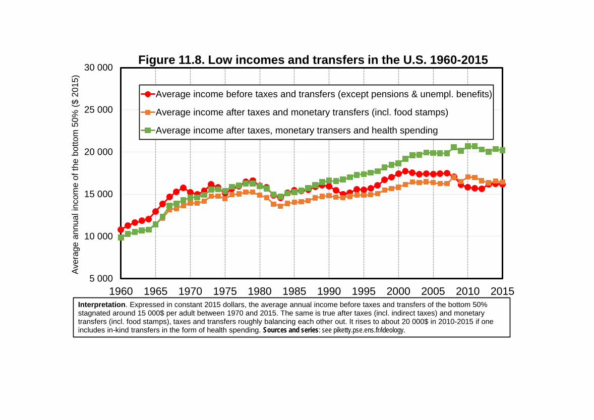
5 000
10 000
15 000
20 000
25 000
30 000
1960 1965 1970 1975 1980 1985 1990 1995 2000 2005 2010 2015
Aver
age
annu
al in
com
e of
the
botto
m 5
0% ($
201
5)Figure 11.8. Low incomes and transfers in the U.S. 1960-2015
Average income before taxes and transfers (except pensions & unempl. benefits)
Average income after taxes and monetary transfers (incl. food stamps)
Average income after taxes, monetary transers and health spending
Interpretation. Expressed in constant 2015 dollars, the average annual income before taxes and transfers of the bottom 50% stagnated around 15 000$ per adult between 1970 and 2015. The same is true after taxes (incl. indirect taxes) and monetary transfers (incl. food stamps), taxes and transfers roughly balancing each other out. It rises to about 20 000$ in 2010-2015 if one includes in-kind transfers in the form of health spending. Sources and series: see piketty.pse.ens.fr/ideology.et

2
4
8
16
1990 1995 2000 2005 2010 2015
Ratio
betw
een
aver
age
incom
es of
top 1
0% an
d bott
om 50
%Figure 11.9. Primary inequality and redistribution: U.S. vs France
Inequality before taxes and transfers (U.S.)
Inequality after taxes and transfers (U.S.)
Inequality before taxes and transfers (France)
Inequality after taxes and transfers (France)
Interpretation. In France, the ratio between the average income before taxes and transfers of the top decile (the 10% highest incomes) and of the bottom half (the 50% lowest incomes) rose from 6,4 in 1990 to 7,4 in 2015. In the U.S., this same ratio rose from 11,5 to 18,7. In both countries, taking into account taxes and monetary transfers (incl. food stamps and housing benefits) reduces inequality by about 20%-30%. Note: the distribution is that of annual income per adult. Sources and series: see piketty.pse.ens.fr/ideology.et

$0,0
$1,2
$2,4
$3,6
$4,8
$6,0
$7,2
$8,4
$9,6
$10,8
$12,0
$13,2
0 €
1 €
2 €
3 €
4 €
5 €
6 €
7 €
8 €
9 €
10 €
11 €
1950 1955 1960 1965 1970 1975 1980 1985 1990 1995 2000 2005 2010 2015 2020
Hou
rly m
inim
um w
age
Figure 11.10. The minimum wage: U.S. vs France 1950-2019
France (2019 euros, left scale)
U.S. (2019 dollars, right scale)
,
Interpretation. Converted into 2019 purchasing power, the federal minimum wage increased from 4,25$ per hour in 1950 to 7,25$ in 2019 in the U.S., while the national minimum wage (Smig in 1950 and then Smic beginning in 1970) rose from 2,23€ per hour in 1950 to 10,03€in 2019. Both scales are based upon purchasing power parity (1,2$ for 1€ in 2019). Sources and series: see piketty.pse.ens.fr/ideology.et
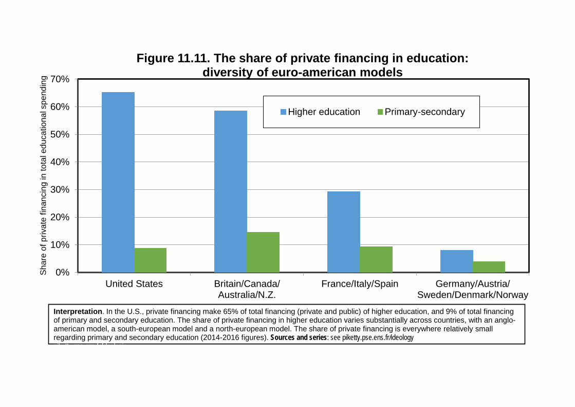
0%
10%
20%
30%
40%
50%
60%
70%
United States Britain/Canada/Australia/N.Z.
France/Italy/Spain Germany/Austria/Sweden/Denmark/Norway
Sha
re o
f priv
ate
finan
cing
in to
tal e
duca
tiona
l spe
ndin
g
Figure 11.11. The share of private financing in education: diversity of euro-american models
Higher education Primary-secondary
Interpretation. In the U.S., private financing make 65% of total financing (private and public) of higher education, and 9% of total financingof primary and secondary education. The share of private financing in higher education varies substantially across countries, with an anglo-american model, a south-european model and a north-european model. The share of private financing is everywhere relatively smallregarding primary and secondary education (2014-2016 figures). Sources and series: see piketty.pse.ens.fr/ideologySources et séries: voir piketty.pse.ens.fr/ideologie

11%
12%
13%
14%
15%
16%
17%
18%
19%
20%
0,8%
1,0%
1,2%
1,4%
1,6%
1,8%
2,0%
2,2%
2,4%
2,6%
1870-1910 1910-1950 1950-1990 1990-2020
Sha
re o
f top
per
cent
ile in
tota
l inc
ome
Ann
ual g
row
th ra
te o
f per
cap
ital n
atio
nal i
ncom
e
Figure 11.12. Growth and inequality in the U.S. 1870-2020
Growth (left axis) Inequality (right axis)
Interpretation. in the U.S., the growth rate of per capita national income dropped from 2,2% per year between 1950 and 1990 to 1,1% between 1990 and 2020, while the share of the top percentile (the 1% highest incomes) in national income rose from 12% to 18% over the same period. Sources and series: see piketty.pse.ens.fr/ideologySources et séries: voir piketty.pse.ens.fr/ideologie
Source: calculs de l'auteur à partir des enquêtes post électorales 1956 2017 (élections présidentielles et législatives)

0%
10%
20%
30%
40%
50%
60%
70%
80%
90%
0,8%
1,0%
1,2%
1,4%
1,6%
1,8%
2,0%
2,2%
2,4%
2,6%
1870-1910 1910-1950 1950-1990 1990-2020
Top
mar
gina
l rat
e ap
plie
d to
the
high
est i
ncom
es
Ann
ual g
row
th ra
te o
f per
cap
ita n
atio
nal i
ncom
e
Figure 11.13. Growth and progressive taxation in the U.S. 1870-2020
Growth (left axis) Progressive taxation (right axis)
Interpretation. in the U.S., the growth rate of per capita national income dropped from 2,2% per year between 1950 and 1990 to 1,1% between 1990 and 2020, while the top marginal tax rate applied to the highest incomes dropped from 72% to 35% over the same period. Sources and series: see piketty.pse.ens.fr/ideologySources et séries: voir piketty.pse.ens.fr/ideologie
Source: calculs de l'auteur à partir des enquêtes post électorales 1956 2017 (élections présidentielles et législatives)

7%
9%
11%
13%
15%
17%
19%
21%
23%
0,4%
0,8%
1,2%
1,6%
2,0%
2,4%
2,8%
3,2%
3,6%
1870-1910 1910-1950 1950-1990 1990-2020
Sha
re o
f top
per
cent
ile in
tota
l inc
ome
Ann
ual g
row
th ra
te o
f per
cap
ital n
atio
nal i
ncom
e
Figure 11.14. Growth and inequality in Europe 1870-2020
Growth (left axis) Inequality (right axis)
Interpretation. In Western Europe, the growth rate of per capita national income dropped from 3,3% per year between 1950 and 1990 to 0,9% per year between 1990 and 2020, while the share of the top percentle (the 1% highest incomes) in national income rose from 8% to 11% over the same period (average Germany-Britain-France). Sources and series: see piketty.pse.ens.fr/ideologySources et séries: voir piketty.pse.ens.fr/ideologie

0%
10%
20%
30%
40%
50%
60%
70%
80%
90%
0,4%
0,8%
1,2%
1,6%
2,0%
2,4%
2,8%
3,2%
3,6%
4,0%
1870-1910 1910-1950 1950-1990 1990-2020
Top
mar
gina
l tax
rate
app
lied
to th
e hi
ghes
t inc
omes
Ann
ual g
row
th ra
te o
f per
cap
ita n
atio
nal i
ncom
e
Figure 11.15. Growth and progressive taxation in Europe 1870-2020
Growth (left axis) Progressive taxation (right axis)
Interpretation. In Western Europe, the growth rate of per capita national income dropped from 3,3% per year between 1950 and 1990 to 0,9% per year between 1990 and 2020, while the top marginal tax rate applied to the highest incomes dropped from 98% to 49% over the same period (average Germany-Britain-France). Sources and series: see piketty.pse.ens.fr/ideologySources et séries: voir piketty.pse.ens.fr/ideologie
Source: calculs de l'auteur à partir des enquêtes post-électorales 1956-2017 (élections présidentielles et législatives)

0%
10%
20%
30%
40%
50%
60%
70%
80%
90%
100%
P0-30 P30-40 P40-50 P50-60 P60-70 P70-80 P80-90 P90-95 P95-99 P99-99.5 P99.5-99.9
P99.9-100
Figure 11.16. Composition of income (France 2015)
9 800 € 26 000 € 34 500 € 50 900 € 102 600 € 193 600 € 1 286 100 €
Capital income(dividends, interest, rent,..)
Labour income(wages and pensions)
Mixed income (self-employed)
Interpretation. In France in 2015 (as in most countries where data are available), bottom and middle incomes are mostly made of labour income, while the highest incomes mostly consist of capital income (especially dividends). Note: the distribution shown here is annual income per adult, before taxes but pensions and unemployment insurance. Sources and series: see piketty.pse.ens.fr/ideology.et

0%
10%
20%
30%
40%
50%
60%
70%
80%
90%
100%
P0-10 P10-20 P20-30 P30-40 P40-50 P50-60 P60-70 P70-80 P80-90 P90-95 P95-99 P99-99.5
P99.5-99.9
P99.9-100
Figure 11.17. Composition of property (France 2015)
Real estate assets (housing), net of debt
Business assets (self-employed)
Financial assets (stocks,bonds, etc. except cash and deposits)
Cash, deposits
2 450 €€ 23 000 € 111 000 € 198 000 € 497 000 € 2 368 000 € 15 650 000 €
Interpretation. In France in 2015 (as in most countries where data are available), small fortunes consist primarily cash and bank deposits,medium fortunes of real estate, and large fortunes of financial assets (mainly stocks). Note: the distribution shown here is per adult wealth (wealth of couples divided by two). Sources and series: see piketty.pse.ens.fr/ideology.et

0%5%
10%15%20%25%30%35%40%45%50%55%60%65%
Income from capital Total income Income from labour
Sha
re o
f eac
h gr
oup
in th
e to
tal
Figure 11.18. Inequalities with respect to capital & labour (France 2015)
Bottom 50%
Next 40%
Top 10%
Interpretation. The 10% highest capital incomes account for 66% of total capital income, vs 5% for the 50% lowest and 29% for the next 40%. Regarding labour income, these shares are respectively 27%, 24% and 49%. Note. The distributions shown here are per adult annual income (the incomes of couples were divided by two). Sources and series: see piketty.pse.ens.fr/ideologie.et
Top 10%
Top 10% Next 40%
Next 40%
Bottom 50%
Bottom 50%

0%
10%
20%
30%
40%
50%
60%
0 10 20 30 40 50 60 70 80 90 95 99 995 999 9999
Tota
l effe
ctiv
e ta
x ra
te a
s a
func
tion
of in
cim
e pe
rcen
tile
Figure 11.19. Profile of tax structure, France 2018
Indirect taxes (VAT etc.)
Social security and other social contributions
Taxes on capital (IS, TF, ISF, etc.)
Proportional income taxes (CSG, etc.)
Progressiveincome tax
Interpretation. In France in 2018, the total effective tax rate is about 45% for bottom incomes groups, 50%-55% for middle and upper-middle incomes groups, and 45% for the highest income groups. Note: the distribution reported here is that of annual factor income among adults aged 25 to 60 year-old and working at least part-time. Sources and series: see piketty.pse.ens.fr/ideology.et

20%
25%
30%
35%
40%
45%
50%
1900 1910 1920 1930 1940 1950 1960 1970 1980 1990 2000 2010
Sha
re o
f top
dec
ile in
tota
l nat
iona
l inc
ome
Figure 12.1. Income inequality in Russia, 1900-2015
Russia
United States
Europe
Interpretation. The share of the top decile (the 10% highest incomes) in total national income was on average about 25% in soviet Russia, i.e. at a lower level than in Western Europe and the U.S., before rising to 45%-50% after the fall of communism, surpassing both Europe and the U.S.. Sources and series: see piketty.pse.ens.fr/ideology.et

0%
5%
10%
15%
20%
25%
1900 1910 1920 1930 1940 1950 1960 1970 1980 1990 2000 2010
Sha
re o
f top
per
cent
ile in
tota
l nat
iona
l inc
ome
Figure 12.2. The top percentile in Russia 1900-2015
Russia
United States
Europe
Interpretation. The share of the top percentile (the 1% highest incomes) in total national income was on average about 5% in soviet Russia, i.e. at a lower level than in Western Europe and the U.S., before rising to 20%-25% after the fall of communism, surpassing both Europe and the U.S.. Sources and series: see piketty.pse.ens.fr/ideology.et

30%
35%
40%
45%
50%
55%
60%
65%
70%
75%
80%
1870 1880 1890 1900 1910 1920 1930 1940 1950 1960 1970 1980 1990 2000 2010
Figure 12.3. The income gap between Russia & Europe 1870-2015
Ratio between average national incomein Russia and in Western Europe
Interpretation. Expressed in purchasing power parity, average national income per adult in Russia was about 35%-40% of Western European average (Germany-France-Britain) between 1870 and 1910, before rising between 1920 and 1950, and stabilizing at about 60% of West European level between 1950 and 1990. Sources and series: see piketty.pse.ens.fr/ideology.et

0%
10%
20%
30%
40%
50%
60%
70%
80%
90%
100%
110%
120%
1990 1995 2000 2005 2010 2015
Rus
sian
fina
ncia
l ass
ets
held
in ta
x ha
vens
(% n
atio
nal i
ncom
e)
Figure 12.4. Capital flight from Russia to tax havens
High estimate
Middle estimate
Low estimate
Interpretation. Given the rising gap between cumulated Russian trade surpluses (close to 10% of national income per year on average between 1993 and 2015) and official foreign reserves (only 30% of national income in 2015), and using various hypotheses on yields obtained, one can estimate that Russian financial assets held in tax havens are between 70% and 110% of national income in 2015,with an average value of 90%. Sources and series: see piketty.pse.ens.fr/ideology.et

0%
10%
20%
30%
40%
50%
60%
United States Europe Latin America Africa Russia Gulf countries
Shar
e of
fina
ncia
l ass
ets
held
in ta
x ha
vens
(201
5)
Figure 12.5. Financial assets held in tax havens
Interpretation. By exploiting anomalies in international financial statistics and the breakdowns by country of residence published by the Bank of International Settlements and the Swiss National Bank, one can estimate that the share of financial assets held via tax havens reaches 4% in the U.S., 10% in Europe and 50% in Russia. These estimates exclude non-financial assets (such as real estate) and financial assets unreported to BIS and SNB and should be considered minimum estimates. Sources and series: see piketty.pse.ens.fr/ideology.012, le candidat de gauche (Hollande) obtient 47% des voix parmi les électeurs sans diplôme (en dehors du certificat d'études primaires), 50% parmi les diplômés du secondaire (Bac, Brevet, Bep, etc.), 53% parmi les diplômés du supérieur court (bac+2) en 2012, le candidat de gauche (Hollande) obtient

-10%
0%
10%
20%
30%
40%
50%
60%
70%
80%
1978 1982 1986 1990 1994 1998 2002 2006 2010 2014 2018
Sha
re o
f net
ubl
ic c
apita
l in
natio
nal c
apita
lFigure 12.6. The fall of public property, 1978-2018
China U.S.Britain FranceGermany Japan
Interpretation. The share of public capital (public assets net of debt, all governement levels and asset categories combined: companies, buildings, land, financial assets, etc.) in national capital (i.e. the sum of public and private capital) was about 70% in China in 1978, and it has stabilized around 30% since the mid-2000s. This share was around 15%-30% in capitalist countries in the 1970s and is near zero or negative in the late 2010s. Sources and series: see piketty.pse.ens.fr/ideology.et

0%
10%
20%
30%
40%
50%
60%
70%
80%
90%
100%
1978 1982 1986 1990 1994 1998 2002 2006 2010 2014 2018
Sha
re in
tota
l cap
ital o
f Chi
nese
com
pani
esFigure 12.7. Ownership of Chinese firms, 1978-2018
Public (Chinese State)
Private (Chinese households)
Foreign (rest of the world)
Interpretation. The Chinese State (all governement levels combined) owned in 2017 about 55% of total capital of Chinese firms (both listed and unlisted, of all sizes and all sectors), vs 33% for Chinese households and 12% for foreign investors. The foreign share has diminished since 2003, and that of Chinese households increased, while that of the Chinese State stabilized around 55%. Sources and series: see piketty.pse.ens.fr/ideology.et

10%
15%
20%
25%
30%
35%
40%
45%
50%
1980 1985 1990 1995 2000 2005 2010 2015
Sha
re o
f eac
h gr
oup
in to
tal n
atio
nal i
ncom
eFigure 12.8. Inequality in China, Europe and the U.S. 1980-2018
ChinaUnited StatesEurope
Interpretation. Income inequality increased strongly in China between 1980 and 2018, but remains according to available sources lower than in the U.S. (but higher than in Europe). Sources and series: see piketty.pse.ens.fr/ideology.et
Top 10% share
Bottom 50% share

10%
15%
20%
25%
30%
35%
40%
45%
50%
1980 1985 1990 1995 2000 2005 2010 2015
Sha
re o
f eac
h gr
oup
in to
tal n
atio
nal i
ncom
eFigure 12.9. Regional inequality: United States vs Europe
United StatesEurope (west + east)Europe (west)
Interpretation. Income inequality is higher when one combines Western and Eastern Europe (population 540 millions inhabitants) than if one looks only at Western Europe (420 millions) and excludes Eastern Europe (120 millions), given the persistent average income gaps between West and East. In any case, inequality is much smaller than in the United States (320 millions inhabitants). Sources and series: see piketty.pse.ens.fr/ideology.et
Top 10% share Bottom 50%
share

0%
1%
2%
3%
4%
5%
6%
7%
8%
Poland Hungary Czech Republic Slovakia
Aver
age
annu
al fl
ows
2010
-201
6 (%
GD
P)
Figure 12.10. Inflows and outflows in Eastern Europe 2010-2016
Inflows of transfers fromthe EU
Outflows of profits andother property income
Interpretation. Between 2010 and 2016, the annual flow of net transfers from the EU (difference between total spending received and total contributions paid to EU budget) was equal to 2,7% of GDP per year on average in Poland. Over the same period, the outflow of profits and other property income (net of the corresponding inflow) was 4,7% of GDP. For Hungary, the same figures were 4,0% and 7,2%. Sources and series: see piketty.pse.ens.fr/ideology.hSourcnet e annual net transfers from the European Union, that is, the difference between the totality of expenditure received and the contributions paid to the EU budget, were appreciably lower: 2.7% of the G.

13
25
50
100
200
400
800
1600
3200
6400
1700 1740 1780 1820 1860 1900 1940 1980 2020 2050
Pop
ulat
ion
in m
illion
s in
habi
tant
s
Figure 13.1. Population by continents, 1700-2050
Asia Europe
Africa America
Interpretation. Around 1700, world population was about 600 millions inhabitants, of whom 400 million lived in Asia and the Pacific, 120 in Europe and Russia, 60 in Africa and 15 in America. In 2050, according to UN projections, it will be about 9,3 billions inhabitants, with 5,2 in Asia-Pacific, 2,2 in Africa, 1,2 in the Americas and 0,7 in Europe-Russia. Sources and series: see piketty.pse.ens.fr/ideology.et

0%
10%
20%
30%
40%
50%
60%
70%
Europe China Russia U.S. India Brasil MiddleEast
SouthAfrica
Qatar
Sha
re o
f top
dec
ile in
tota
l nat
iona
l inc
ome
Figure 13.2. Global inequality regimes (2018)
Interpretation. In 2018, the share of the top decile (the 10% highest incomes) in national income was 34% in Europe (EU+), 41% in China, 46% in Russia, 48% in the U.S., 55% in India, 56% in Brasil, 64% in the Middle East, 65% in South Africa and 68% in Qatar. Sources and series: see piketty.pse.ens.fr/ideology.012, le candidat de gauche (Hollande) obtient 47% des voix parmi les électeurs sans diplôme (en dehors du certificat d'études primaires), 50% parmi les diplômés du secondaire (Bac, Brevet, Bep, etc.), 53% parmi les diplômés du supérieur court (bac+2) en 2012, le candidat de gauche (Hollande) obtient 47% des voix parmi les électeurs sans diplôme (en dehors du certificat d'études primaires), 50% parmi

0%
10%
20%
30%
40%
50%
60%
Europe (540 millions) United States (320m) Middle East (420m)
Shar
e of to
tal in
come
rece
ived b
y top
10%
, nex
t 40%
and b
ottom
50%
Figure 13.3. Inequality in 2018: Europe, U.S., Middle East
Bottom 50%
Next 40%
Top 10%
Interpretation. The share of the 10% highest incomes is 64% of total income in the Middle East (pop. 420 million), compared to 9% for the bottom 50% share. In Europe (enlarged EU, pop. 540 million) these two shares are 34% and 21%. In the United States (pop.320 million) they are 47% and 13%. Sources and series: see piketty.pse.ens.fr/ideology.et
Top 10%
Top 10%
Next 40%
Next 40%
Bottom 50%
Bottom 50%

0%
5%
10%
15%
20%
25%
30%
Europe China United States Middle East
Shar
e of to
tal in
come
rece
ived b
y the
botto
m 50
% an
d the
top 1
%Figure 13.4. Global inequality regimes (2018):
the bottom 50% vs the top 1%
Bottom 50%
Top 1%
Bottom 50%
Interpretation. The share of bottom 50% highest incomes is only 9% of total income in the Middle East, vs 30% for the top 1% share. In Europe, these two shares are 21% and 11%. In China they are 15% and 14%, and in the U.S; they are 13% and 20%. Sources and series: see piketty.pse.ens.fr/ideology.et
Top 1%
Top 1%
Bottom 50%
Top 1%
Bottom 50%
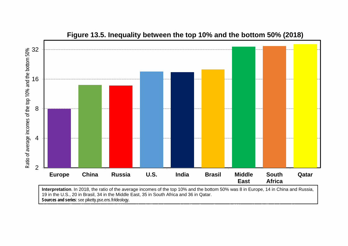
2
4
8
16
32
Europe China Russia U.S. India Brasil MiddleEast
SouthAfrica
Qatar
Ratio
of av
erag
e inc
omes
of th
e top
10%
and t
he bo
ttom
50%
Figure 13.5. Inequality between the top 10% and the bottom 50% (2018)
Interpretation. In 2018, the ratio of the average incomes of the top 10% and the bottom 50% was 8 in Europe, 14 in China and Russia, 19 in the U.S., 20 in Brasil, 34 in the Middle East, 35 in South Africa and 36 in Qatar. Sources and series: see piketty.pse.ens.fr/ideology.012, le candidat de gauche (Hollande) obtient 47% des voix parmi les électeurs sans diplôme (en dehors du certificat d'études primaires), 50% parmi les diplômés du secondaire (Bac, Brevet, Bep, etc.), 53% parmi les diplômés du supérieur court (bac+2) en 2012, le candidat de gauche (Hollande) obtient 47% des voix parmi les électeurs sans diplôme (en dehors du certificat d'études

10
20
40
80
160
Europe China Russia U.S. India Brasil MiddleEast
SouthAfrica
Qatar
Ratio
of av
erag
e inc
omes
of th
e top
1% an
d the
botto
m 50
%Figure 13.6. Inequality between the top 1% and the bottom 50% (2018)
Interpretation. In 2018, the ratio of the average incomes of the top 1% and the bottom 50% was 25 in Europe, 46 in China, 61 in Russia, 80 in the U.S., 72 in India, 85 in Brasil, 161 in the Middle East, 103 in South Africa and 154 in Qatar. Sources and series: see piketty.pse.ens.fr/ideology.012, le candidat de gauche (Hollande) obtient 47% des voix parmi les électeurs sans diplôme (en dehors du certificat d'études primaires), 50% parmi les diplômés du secondaire (Bac, Brevet, Bep, etc.), 53% parmi les diplômés du supérieur court (bac+2) en 2012, le candidat de gauche (Hollande) obtient 47% des voix parmi les électeurs sans diplôme (en dehors du certificat d'études

0%
5%
10%
15%
20%
25%
30%
35%
40%
45%
50%
55%
60%
North America Europe China Rest of the world
Sha
re o
f eac
h re
gion
in g
loba
l em
issi
ons
Figure 13.7. The global distribution of carbon emissions 2010-2018
Total carbon emissionsIndividual carbon emissions higher than global averageEmissions higher than 2,3x global average (top 10%)Emissions higher than 9,1x global average (top 1%)
Interpretation. The share of North America (U.S.-Canada) in total global emissions (direct and indirect) was 21% on average in 2010-2018; thisshare rises to 36% if one looks at emissions greater than global average (6,2t CO2e per year), 46% for emissions above 2,3 times the global average (i.e. the top 10% of world emitters, accounting for 45% of total emissions, compared to 13% for the bottom 50% of world emitters), and 57% of those emitting over 9,1 times the global average (i.e. the top 1% of world emitters, accounting for 14% of total emisssions). Sources and series: see piketty.pse.ens.fr/ideology.et

35%
40%
45%
50%
55%
60%
65%
70%
75%
80%
85%
90%
95%
1900 1910 1920 1930 1940 1950 1960 1970 1980 1990 2000 2010
Sha
re o
f top
dec
ile in
tota
l priv
ate
prop
erty
Figure 13.8. Top decile wealth share: rich and emerging countries
United States ChinaIndia RussiaBritain France
Reading. The share of the top decile (the 10% largest wealth owners) in total private property (all assets combined: real estate, business and financial assets, net of debt) increased strongly in China, Russia, India and the United States since the 1980s-1990s, and to a lesser extent in Britain and France. Sources and series: see piketty.pse.ens.fr/ideology.

5%10%15%20%25%30%35%40%45%50%55%60%65%70%
1900 1910 1920 1930 1940 1950 1960 1970 1980 1990 2000 2010
Sha
re o
f top
per
cent
ile in
tota
l priv
ate
prop
erty
Figure 13.9. Top percentile wealth share: rich & emerging countries
United States ChinaIndia RussiaBritain France
Reading. The share of the top percentile (the 1% largest wealth owners) in total private property (all assets combined: real estate,business and financial assets, net of debt) increased strongly in China, Russia, India and the United States since the 1980s-1990s, and to a lesser extent in Britain and France. Sources and series: see piketty.pse.ens.fr/ideology.
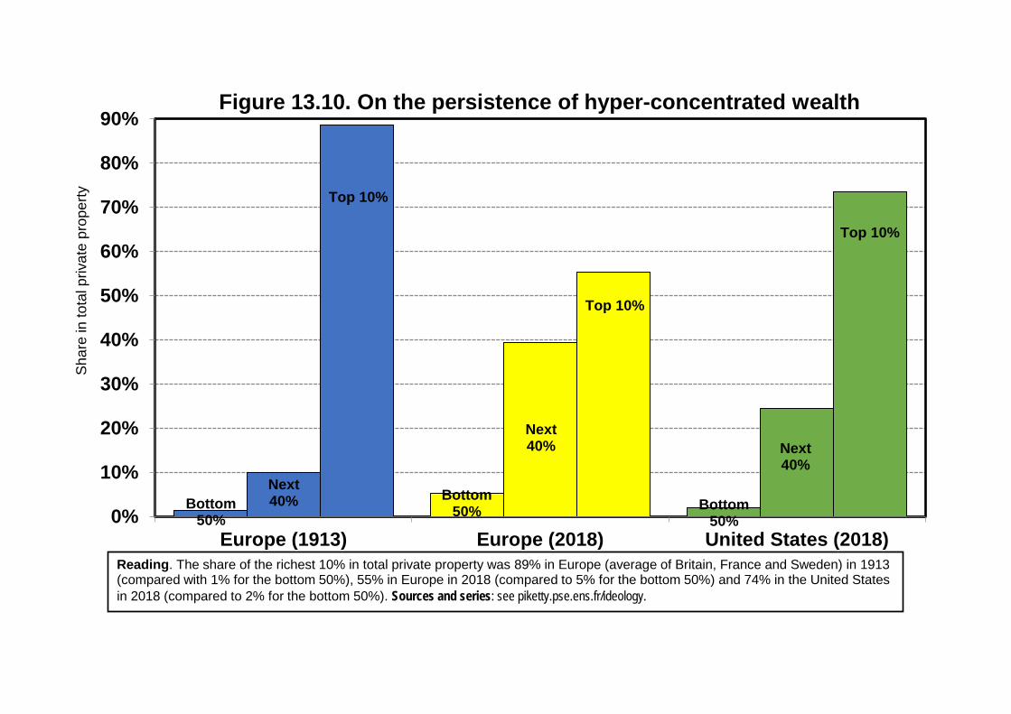
0%
10%
20%
30%
40%
50%
60%
70%
80%
90%
Europe (1913) Europe (2018) United States (2018)
Sha
re in
tota
l priv
ate
prop
erty
Figure 13.10. On the persistence of hyper-concentrated wealth
Bottom 50%
Next 40%
Top 10%
Reading. The share of the richest 10% in total private property was 89% in Europe (average of Britain, France and Sweden) in 1913 (compared with 1% for the bottom 50%), 55% in Europe in 2018 (compared to 5% for the bottom 50%) and 74% in the United Statesin 2018 (compared to 2% for the bottom 50%). Sources and series: see piketty.pse.ens.fr/ideology.et
Top 10%
Top 10%
Next 40%
Next 40%
Bottom 50% Bottom
50%

0%
5%
10%
15%
20%
25%
30%
35%
40%
45%
50%
1970 1975 1980 1985 1990 1995 2000 2005 2010 2015 2020 2025
Pro
porti
on o
f wom
en a
mon
g hi
gh in
com
es in
Fra
nce
Figure 13.11. The persistence of patriarchy in France in the 21st
centuryProportion of women in top
50%
Top 10%
Top 1%
Top 0.1%
Proportion of women in top 1%: 10% in 1995, 16% in 2015, 50% in 2102 ?
Top 0.1%: 50% women in 2144?
Interpretation. The proportion of women in the top percentile (top 1%) of the distribution of labour income (wages and self-employment income) increased from 10% in 1995 to 16% in 2015, and should reach 50% by 2102 if the trend continues at the same speed as during the 1995-2015 period. For the top 0,1%, parity could wait until 2144. Sources and series: see piketty.pse.ens.fr/ideology.

0%
5%
10%
15%
20%
25%
30%
35%
40%
45%
1970-1979 1980-1989 1990-1999 2000-2009 2010-2018
Tax
reve
nues
as
% G
DP
Figure 13.12. Tax revenues and trade liberalization 1970-2018
High-income countries: total tax revenues
including taxes on international trade
Low-income countries: total tax revenues
including taxes on international trade
Interpretation. In low-income countries (bottom third: Subsaharan Africa, South Asia, etc.), tax revenues dropped from 15,6% of GDP in 1970-1979 to 13,7% in 1990-1999 and 14,5% in 2010-2018, partly due to the uncompensated fall in customs duties and other taxes on international trade (which raised 5,9% of GDP in 1970-1979, 3,9% in 1990-1999 and 2,8% in 2010-2018). In high-income countries (top third: Europe, North America, etc.), customs dutiers were already very small at the beginning of the period and tax revenues kept rising before stabilizing. Sources and series: see piketty.pse.ens.fr/ideology.et

0%5%
10%15%20%25%30%35%40%45%50%55%60%
1900 1910 1920 1930 1940 1950 1960 1970 1980 1990 2000 2010
Tota
l cen
tral b
ank
asse
ts a
s %
GD
PFigure 13.13. The size of central bank balance sheets 1900-2018
Average rich countries(17 countries)Euro zone 1999-2018 (averageGermany-France 1900-1998)United States (Federal Reserve)
Interpretation. Total assets of the European Central Bank (ECB) rose from 11% of euro zone GDP on 31/12/2004 to 41% on 31/12/2018. The evolution 1900-1998 indicates the average obtained for the blance sheets of the German and French central banks (with peaks equal to 39% in 1918 and 62% in 1944). Total assets of the Federal Reserve (created in 1913) rose from 6% of GDP in 2007 to 26% at th end of 2014. Note. The average of rich countries is the arithmetic average of the 17 following countries: Australia, Belgium, Britain, Canada, Denmark, France, Finland, Germany, Holland, Italy, Japan, Norway, Portugal, Spain, Sweden, Switzerland, U.S.). Sources and series: see piketty.pse.ens.fr/ideology.

0%
10%
20%
30%
40%
50%
60%
70%
80%
90%
100%
110%
1900 1910 1920 1930 1940 1950 1960 1970 1980 1990 2000 2010
Tota
l cen
tral b
ank
asse
ts a
s %
GD
PFigure 13.14. Central banks and financial globalization
SwitzerlandJapanAverage rich countries (17 countries)Euro zoneUnited States (Federal Reserve)
Interpretation. Total assets of the central banks of rich countries rose from 13% of GDP on 31/12/2000 to 51% on 31/12/2018. The assets of the central banks of Japan and Switzerland exceeded 100% of GDP in 2017-2018. Note. The average of rich countries is the arithmetic average of the 17 following countries: Australia, Belgium, Britain, Canada, Denmark, France, Finland, Germany, Holland, Italy, Japan, Norway, Portugal, Spain, Sweden, Switzerland, U.S.). Sources and series: see piketty.pse.ens.fr/ideology.

Annual average real growth rate 1987-2017
(after deduction of inflation)World U.S.-Europe-China
The one hundred-millionth richest (Forbes) 6,4% 7,8%
The one twenty-millionth richest (Forbes) 5,3% 7,0%
The top 0,01% (WID.world) 4,7% 5,7%
The top 0,1% (WID.world) 3,5% 4,5%
The top 1% (WID.world) 2,6% 3,5%
Per adult average wealth 1,9% 2,8%
Per adult average income 1,3% 1,4%
Total adult population 1,9% 1,4%
GDP or total income 3,2% 2,8%
Interpretation. Between 1987 and 2017, the average wealth of the one hundred-millionth richest individuals in the world(i.e. about 30 individuals out of 3 billions adults in 1987, and 50 out of 5 billions in 2017) grew by 6,4% a year globally; theaverage wealth of the 0,01% richest individuals (about 300 000 individuals in 1987, 500 000 in 2017) grew by 4,7% a year,and average global wealth by 1,9% a year. The rise of very top wealth holders has been even more marked if weconcentrate on U.S.-Europe-China. Sources: see piketty.pse.ens.fr/ideology
Table 13.1. The rise of top global wealth holders, 1987-2017

-32%-28%-24%-20%-16%-12%-8%-4%0%4%8%
12%16%20%24%28%32%
1955 1960 1965 1970 1975 1980 1985 1990 1995 2000 2005 2010 2015 2020
Figure 14.1. Social cleavages & political conflict in France 1955-2020Difference between % vote for left parties among the top 10% educationvoters and the bottom 90% education voters (after controls)Difference between % vote for left parties among the top 10% incomevoters and the bottom 90% income voters (after controls)Difference between % vote for left parties among the top 10% wealthvoters and the bottom 90% wealth voters (after controls)
Interpretation. In the 1950-1970 period, the vote for left-wing parties (socialists-communists-radicals-greens) was associated to voters with the lowest education degrees and the lowest levels of income and wealth; in the 1990-2010 period, it became associated to the voters with the highest education degrees. Note: fine lines indicate 90% confidence intervals. Sources and series: see piketty.pse.ens.fr/ideology.alculs de l'auteur à partir des enquêtes post-électorales 1956-2017 (élections présidentielles et législatives). Lecture: en 1956 les partis de gauche (SFIO PS PCF MRG divers gauche et écologistes extrême gauche) obtiennent un score 12 point

-24%-20%-16%-12%
-8%-4%0%4%8%
12%16%20%24%
1945 1950 1955 1960 1965 1970 1975 1980 1985 1990 1995 2000 2005 2010 2015 2020
Figure 14.2. Electoral left in Europe and the U.S. 1945-2020: from the workers' party to the party of the highly educated
U.S.: difference between % vote democrat among the top 10%education voters and the bottom 90% education voters (after controls)France: same difference with the vote for left parties
Britain: same difference with the vote for labour party
Interpretation. In the 1950-1970 period, the vote for the democrats in the US., left-wing parties (socialists-communists-radicals-greens) in France and the labour party in Britain was associated to voters with the lowest education; in the 1990-2010 period, it became associated to the voters with the highest education degrees. Sources and series: see piketty.pse.ens.fr/ideology.alculs de l'auteur à partir des enquêtes post-électorales 1956-2017 (élections présidentielles et législatives).

0%4%8%
12%16%20%24%28%32%36%40%44%48%52%56%60%64%
1945 1950 1955 1960 1965 1970 1975 1980 1985 1990 1995 2000 2005 2010 2015 2020
Figure 14.3. Legislative elections in France, 1945-2017
Electoral left (SFIO-PS, PCF, radicals, various left, greens, extreme-left)
Electoral right (MRP, CNIP, UNR, RPR, UDF, UMP, LR, various right, FN, extreme-right)
Other parties (difficult to rank on left-right scale: regionalists, hunters, etc.)
Interpretation. The scores obtained by left-wing parties (socialistes, communistes, radicals, greens and ohter parties from the center-left, left and extreme-left) and right-wing parties (all parties from center-right, right and extreme-right combined) have oscillated between 40% and 58% of the votes in the first rounds of legislative elections conducted in France over the 1945-2017 period. Note: the score obtained by the LREM-MODEM coalition in 2017 (32% of votes) was divided 50-50 between center-left and center-right (see figures 14.4-14.5). Sources and series: see piketty.pse.ens.fr/ideology.de l'auteur à partir des enquêtes post-électorales 1956-2017 (élections présidentielles et législatives). 1956, les partis de gauche (SFIO-PS, PCF, MRG divers gauche et écologistes extrême gauche) obtiennent un score 12 point
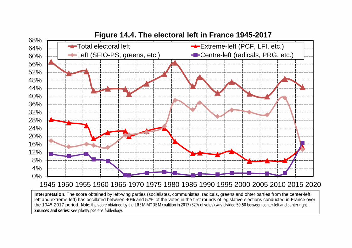
0%4%8%
12%16%20%24%28%32%36%40%44%48%52%56%60%64%68%
1945 1950 1955 1960 1965 1970 1975 1980 1985 1990 1995 2000 2005 2010 2015 2020
Figure 14.4. The electoral left in France 1945-2017Total electoral left Extreme-left (PCF, LFI, etc.)Left (SFIO-PS, greens, etc.) Centre-left (radicals, PRG, etc.)
Interpretation. The score obtained by left-wing parties (socialistes, communistes, radicals, greens and ohter parties from the center-left, left and extreme-left) has oscillated between 40% and 57% of the votes in the first rounds of legislative elections conducted in France over the 1945-2017 period. Note: the score obtained by the LREM-MODEM coalition in 2017 (32% of votes) was divided 50-50 between center-left and center-right. Sources and series: see piketty.pse.ens.fr/ideology.de l'auteur à partir des enquêtes post-électorales 1956-2017 (élections présidentielles et

0%4%8%
12%16%20%24%28%32%36%40%44%48%52%56%60%64%68%
1945 1950 1955 1960 1965 1970 1975 1980 1985 1990 1995 2000 2005 2010 2015 2020
Figure 14.5. The electoral right in France (1945-2017)Total electoral right Center-right (MRP, UDF, UDI, etc.)Right (RPF, RPR, UMP, LR, etc.) Extreme-right (UDCA, FN, etc.)
Interpretation. The score obtained by right-wing parties (all parties from the center-right, right and extreme-right combined) has oscillated between 40% and 58% of the votes in the first rounds of legislative elections conducted in France over the 1945-2017 period. Note: the score obtained by the LREM-MODEM coalition in 2017 (32% of votes) was divided 50-50 between center-left and center-right. Sources and series: see piketty.pse.ens.fr/ideology.de l'auteur à partir des enquêtes post-électorales 1956-2017 (élections présidentielles et législatives). 1956, les partis de gauche (SFIO-PS, PCF,

26%30%34%38%42%46%50%54%58%62%66%70%74%
1965 1970 1975 1980 1985 1990 1995 2000 2005 2010
Figure 14.6. Presidential elections in France, 1965-2012
Left (candidate supported by socialist party (PS) and other left-wing parties)Right (candidate supported by the gaullist party and other right-wing parties)
Interpretation. The scores obtained during the second rounds left-right of French presidential elections reported here are the following 1965 (De Gaulle 55%, Mitterrand 45%), 1974 (Giscard 51%, Mitterrand 49%), 1981 (Mitterrand 52%, Giscard 48%), 1988 (Mitterrand 54%, Chirac 46%), 1995 (Chirac 53%, Jospin 47%), 2007 (Sarkozy 53%, Royal 47%), 2012 (Hollande 52%, Sarkozy 48%). Other second rounds (opposing the right, the center and the extreme-right) were not reported here: 1969 (Pompidou 58%, Poher 42%), 2002 (Chirac 82%, Le Pen 18%), 2017 (Macron 66%, Le Pen 34%). Sources and series: see piketty.pse.ens.fr/ideology.de l'auteur à partir des enquêtes post-électorales 1956-2017 (élections présidentielles et législatives). 1956, les partis de gauche (SFIO-PS, PCF, MRG, divers gauche et
De Gaulle 55% Mitterrand 45%
Mitterrand 54% Chirac 46%
Hollande 52% Sarkozy 48%

30%
35%
40%
45%
50%
55%
60%
65%
70%
75%
80%
85%
90%
1945 1950 1955 1960 1965 1970 1975 1980 1985 1990 1995 2000 2005 2010 2015 2020
Figure 14.7. The evolution of voter turnout 1945-2020
France (presidential elections)France (legislatives elections)Britain (legislative elections)U.S. (presidential elections)
Interpretation. Voter turnout has been relatively stable around 80%-85% in French presidential elections since 1965 (with however a small fall to 75% in 2017). The fall has been much stronger in legislative elections, which was around 80% until the 1970s, and was less than 50% in 2017. Electoral participation dropped in Britain before rising again since 2010. In the U.S., it has generally fluctuated around 50%-60%. Sources and series: see piketty.pse.ens.fr/ideology.de l'auteur à partir des enquêtes post-électorales 1956-2017 (élections
é id i ll lé i l i ) 1956 l i d h (SFIO PS PCF MRG di h é l i ê h ) b i

-12%
-8%
-4%
0%
4%
8%
12%
16%
20%
24%
1945 1950 1955 1960 1965 1970 1975 1980 1985 1990 1995 2000 2005 2010 2015 2020
Figure 14.8. Voter turnout & social cleavages 1945-2020
U.S.: difference between % electoral participation among the 50%highest income voters and the 50% lowest income votersFrance: same difference
Britain: same difference
Interpretation. During the 1950-1980 period, electoral participation in France and Britain was at most 2%-3% higher among the 50% highest incom voters than among the 50% lowest income voters. This gap rose significantly since the 1980s and reached 10%-12% in the 2010s? thereby approaching the levels historically observed in the U.S. Sources and series: see piketty.pse.ens.fr/ideology.de l'auteur à partir des enquêtes post-électorales 1956-2017 (élections présidentielles et législatives). 1956, les partis de gauche (SFIO-PS, PCF, MRG, divers

20%
25%
30%
35%
40%
45%
50%
55%
60%
65%
1956 1973 1995 2012
Figure 14.9. Left vote vote by level of education, France 1956-2012
Prim.48%
High.44%
Sec. 47%
Prim. 57%
Sec. 49%
High.37%
Sec. 48%
High.49%
Prim. 44% Prim.
47%
Sec. 50%
High. 58%
72% 18%22%48%30%11%47%42%5%23% 26%56%
Interpretation. In the 1956 legislative elections, 57% of voters with no degree or whose highest degree was a primary education degree (certificat d'études primaires) (i.e. 72% of the electorate at the time) voted for left-wing parties (socialists-communists-radicals), vs. 50% of secondary degree holders (23% of the electorate) and 37% of higher education degree holders (5% of the electorate). In the 2012 presidential elections, the education cleavage was totally reversed: the left-wing candidate obtained 58% of the vote in the second round among higher education degree holders, vs 47% of the vote among primary education degree holders. Sources and series: see piketty.pse.ens.fr/ideology.de l'auteur à partir des enquêtes post électorales 1956 2017 (élections présidentielles et législatives) 1956 les partis de gauche (SFIO PS PCF MRG

20%
25%
30%
35%
40%
45%
50%
55%
60%
65%
1956 1958 1962 1965 1967 1973 1974 1978 1981 1986 1988 1993 1995 1997 2002 2007 2012 2017
Vote
for le
ft-wi
ng pa
rties a
s a fu
nctio
n of h
ighes
t deg
ree o
btaine
d
Figure 14.10. The reversal of the education cleavage, France 1956-2017
Primary Secondary Higher education
Interpretation. During the 1950s and 1960s, the vote for left-wing parties (socialists-communists-radicals-greens) was highest among voters with no degree (except primary education degrees), then fell among secondary and higher education degree holders. In the 2000s and 2010s, the pattern is completely reversed. Sources and series: see piketty.pse.ens.fr/ideology.de l'auteur à partir des enquêtes post-électorales 1956-2017 (élections présidentielles et législatives). 1956, les partis de gauche (SFIO-PS, PCF, MRG, divers gauche et écologistes, extrême-

-28%
-24%
-20%
-16%
-12%
-8%
-4%
0%
4%
8%
12%
16%
1955 1960 1965 1970 1975 1980 1985 1990 1995 2000 2005 2010 2015 2020
Figure 14.11. The left and education in France 1955-2020
Difference in the % vote for left-wing parties among higher educationgraduates and non-higher education graduatesAfter controls for age, sexe, family situation
After controls for age, sex, family situation, income, wealth
Interpretation. In 1956, left-wing parties (socialists-communists-radicals) obtained a score that was 17 points lower among higher education graduates than among non-higher education graduates; in 2012, this score was 8 points higher among higher education graduates. Controling for other variables does not affect the trend (only the level). Sources and series: see piketty.pse.ens.fr/ideology.de l'auteur à partir des enquêtes post-électorales 1956-2017 (élections présidentielles et législatives). 1956, les partis de gauche (SFIO-PS, PCF, MRG, divers gauche

10%
20%
30%
40%
50%
60%
70%
80%
D1 D2 D3 D4 D5 D6 D7 D8 D9 D10 Top5% Top1%
% v
ote
left
parti
es a
s a
func
tion
of in
com
e de
cile
Figure 14.12. Political conflict and income, France 1958-2012
1958 1962 1974
1978 1986 1988
1995 2007 2012
Interpretation. In 1978, left-wing parties (socialists-communists-radicals-greens) obtained 46% of the vote among the bottom 10% income voters, 38% among the top 10% income voters and 17% among the top 1% income voters. Generally speaking, the left vote profile is relatively flat among the bottom 90% income voters, and strongly decreasing among the top 10% income voters, especially at the beginning of the period. Note: D1 refers to the 10% lowest incomes, D2 to the next 10%,.., and D10 to the 10% highest incomes. Sources and series: see piketty.pse.ens.fr/ideology.de l'auteur à partir des enquêtes post électorales 1956 2017 (élections présidentielles et législatives) 1956 les partis de gauche (SFIO PS PCF

10%
20%
30%
40%
50%
60%
70%
80%
D1 D2 D3 D4 D5 D6 D7 D8 D9 D10 Top5% Top1%
% v
ote
for l
eft-w
ing
parti
es a
s a
func
tion
of w
ealth
dec
ileFigure 14.13. Political conflict and property, France 1974-2012
1974 1978 1986
1988 1995 2007
2012
Interpretation. In 1978, left-wing parties (socialists-communists-radicals-greens) obtained 69% of the vote among the bottom 10% wealth voters, 23% among the top 10% wealth voters and 13% among the top 1% wealth voters. Generally speaking, the left vote profile with respect to wealth is sharply declining (much more strongly than with respect to income), especially at the beginning of the period. Note: D1 refers to the 10% lowest wealth holders, D2 to the next 10%,.., and D10 to the 10% highest wealth holders. Sources and series: see piketty.pse.ens.fr/ideology.de l'auteur à partir des enquêtes post électorales 1956 2017 (élections présidentielles et législatives) 1956 les partis de gauche (SFIO PS
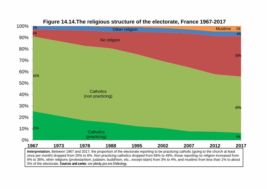
0%
10%
20%
30%
40%
50%
60%
70%
80%
90%
100%
1967 1973 1978 1988 1995 2002 2007 2012 2017
Figure 14.14.The religious structure of the electorate, France 1967-2017
No religion
Catholics(non practicing)
Catholics(practicing)
MuslimsOther religion
66%
49%
25%
3%6%
5%4%
36%
6%
Interpretation. Between 1967 and 2017, the proportion of the electorate reporting to be practicing catholic (going to the church at least once per month) dropped from 25% to 6%. Non practicing catholics dropped from 66% to 49%, those reporting no religion increased from 6% to 36%, other religions (protestantism, judaism, buddhism, etc., except islam) from 3% to 4%, and muslims from less than 1% to about 5% of the electorate. Sources and series: see piketty.pse.ens.fr/ideology.

0%
10%
20%
30%
40%
50%
60%
70%
80%
90%
100%
1967 1973 1978 1988 1995 1997 2002 2007 2012 2017
% v
ote
for l
eft-w
ing
parti
es a
s a
func
tion
of re
porte
d re
ligio
n
Figure 14.15. Political conflict and catholicism: France 1967-2017
Practicing catholics Non practicing catholics No religion
Interpretation. Self-reported practicing and non-practicing catholic voters have always voted less strongly for left-wing parties than voters reporting no religion, but the gap has reduced over time. Sources and series: see piketty.pse.ens.fr/ideology.
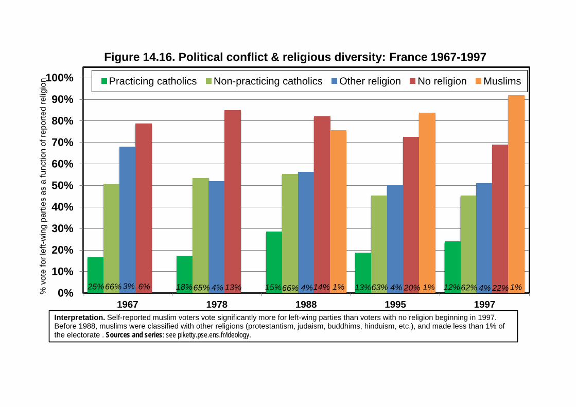
0%
10%
20%
30%
40%
50%
60%
70%
80%
90%
100%
1967 1978 1988 1995 1997
% v
ote
for l
eft-w
ing
parti
es a
s a
func
tion
of re
porte
d re
ligio
n
Figure 14.16. Political conflict & religious diversity: France 1967-1997
Practicing catholics Non-practicing catholics Other religion No religion Muslims
25%66% 3% 6% 18%65% 4% 13% 15% 1%20%4%63%13%1%14%4%66% 1%22%4%62%12%
Interpretation. Self-reported muslim voters vote significantly more for left-wing parties than voters with no religion beginning in 1997. Before 1988, muslims were classified with other religions (protestantism, judaism, buddhims, hinduism, etc.), and made less than 1% of the electorate . Sources and series: see piketty.pse.ens.fr/ideology.

0%
10%
20%
30%
40%
50%
60%
70%
80%
90%
100%
2002 2007 2012 2017
% v
ote
for l
eft-w
ing
parti
es a
s a
func
tion
of re
porte
d re
ligio
n
Figure 14.17. Political conflict & religious diversity: France 2002-2017
Practicing catholics Non-practicing catholics Other religion No religion Muslims
11% 58% 4% 25% 8% 56% 4% 29% 3% 7% 5%35%5%49%6%5%34%4%50%2%
Interpretation. About 80%-90% of self-reported muslim voters vote for left-wing parties in all elections in France since the 1990s. Before 1988, muslims were classified with other religions (protestantism, judaism, buddhims, hinduism, etc.), and made less than 1% of the electorate . Sources and series: see piketty.pse.ens.fr/ideology.

20%
30%
40%
50%
60%
70%
80%
90%
2007 2012
% v
ote
for l
eft-w
ing
parti
es a
s a
func
tion
of fa
mily
orig
ins
Figure 14.18. Political attitudes and origins: France 2007-2012
No foreign origin (no foreign grand-parent)European foreign origin (Spain, Italy, Portugal, etc.)Extra-European foreign origin (North Africa, Subsaharan Africa, etc.)
77%
45%
17% 6% 9%19%72%
49%
71%
49% 49%
77%
Interpretation. In 2012, the socialist candidate received 49% of the vote among voters with no foreign origin (no foreign grand-parent), 49% ofthe vote among voters with European foreign origine (in practice mostly Spain, Italy, Portugal) and 77% of the vote among voters with extra-European foreign origins (in practice mostly North Africa and Subsaharan Africa). Sources and series: see piketty.pse.ens.fr/ideology.

10%
15%
20%
25%
30%
35%
40%
45%
50%
2000 2005 2010 2015 2020
Sha
re o
f eac
h id
eolo
gica
l gro
up in
the
elec
tora
te
Figure 14.19. Borders and property: the four-way ideological divide in France
Internationalists-egalitarians (pro-migrants, pro-poor)Internationalists-inegalitarians (pro-migrants, pro-rich)Nativists-inegalitarians (anti-migrants, pro-rich)Nativists-egalitarians (anti-migrants, pro-poor)
Interpretation. In 2017, 21% of voters can be classified as "internationalists-egalitarians" (they consider that there are not too many migrants and that inequalities between the rich and the poor ought to be reduced); 26% as "nativists-inegalitarians" (they consider that there are too many migrants and that there is no need to reduce the inequalities between the rich and the poor); 23% as "internationalits-inegalitarians" (pro-migrants, pro-rich) and 30% as "nativists-egalitarians" (anti-migrants, pro-poor). Sources and series: see piketty.pse.ens.fr/ideology.

35%
40%
45%
50%
55%
60%
65%
D1 D2 D3 D4 D5 D6 D7 D8 D9 D10
% v
ote
for t
he Y
ES
in th
e re
fern
dum
s of
199
2 an
d 20
05
as a
func
tion
of in
com
e, e
duca
tion
and
wea
lth d
ecile
Figure 14.20. The European cleavage in France: the referenda of 1992 and 2005
1992 (income) 2005 (income)1992 (education) 2005 (education)1992 (wealth) 2005 (wealth)
Interpretation. In the 1992 referendum over the Maastricht treaty ("yes" won with 51%) as well as in the 2005 referendum on the European constitutionnal treaty ("yes" lost with 45%), one observes a very strong social cleavage: top deciles of income, educational degrees and wealth vote strongly for the "yes", while bottom deciles vote for the "no". Note: D1 represents the bottom 10% (for the distribution of income, education or wealth), D2 the next 10%,..., and D10 the top 10%. Sources and series: see piketty.pse.ens.fr/ideology.de l'auteur à partir des

All voters
Melenchon /Hamon
(vote "egalitarian-internationalist")
Macron (vote "inegalitarian-
internationalist")
Fillon (vote "inegalitarian-
nativist")
Le Pen /Dupont-Aignan (vote "egalitarian-
nativist")
100% 28% 24% 22% 26%"There are too many migrants in France"
(% agree) 56% 32% 39% 62% 91%
"In order to achieve social justice, one should take to the rich and give to the poor" (% agree) 51% 67% 46% 27% 61%
Higher education graduates (%) 33% 39% 41% 36% 16%
Monthly income > 4000€ (%) 15% 9% 20% 26% 8%
Home owners (%) 60% 48% 69% 78% 51%
Presidential election 2017 (1st round)
Interpretation. In 2017, 28% of first-round voters voted for Melenchon-Hamon; 32% of them considered that there are too many migrants in France (vs 56% on average among all voters) and 67% that we should take from the rich and give to the poor (vs 51% on average). In that sense this electorate is ideologically "egalitarian-internationalist", while the Macron electorate is "inegalitarian-internationalist" (pro-migrants, pro-rich), the Fillon electorate "inegalitarian-nativist" (anti-migrants, pro-rich) and the Le Pen/Dupont Aignan electorate "egalitarian-nativist" (anti-migrants, pro-poor). Note: the votes for Arthaud/Poutou (2%) and Asselineau/Cheminade/Lassale (2%) were added to Melenchon/Hamon and Fillon. Sources and series: see piketty.pse.ens.fr/ideology.
Table 14.1. Politico-ideological conflict in France 2017: an electorate divided into four quarters
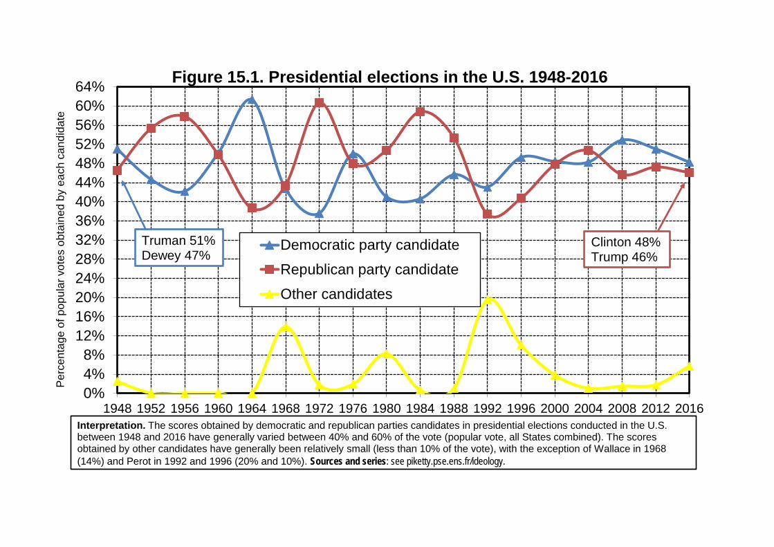
0%4%8%
12%16%20%24%28%32%36%40%44%48%52%56%60%64%
1948 1952 1956 1960 1964 1968 1972 1976 1980 1984 1988 1992 1996 2000 2004 2008 2012 2016
Per
cent
age
of p
opul
ar v
otes
obt
aine
d by
eac
h ca
ndid
ate
Figure 15.1. Presidential elections in the U.S. 1948-2016
Democratic party candidate
Republican party candidate
Other candidates
Clinton 48% Trump 46%
Truman 51% Dewey 47%
Interpretation. The scores obtained by democratic and republican parties candidates in presidential elections conducted in the U.S. between 1948 and 2016 have generally varied between 40% and 60% of the vote (popular vote, all States combined). The scores obtained by other candidates have generally been relatively small (less than 10% of the vote), with the exception of Wallace in 1968 (14%) and Perot in 1992 and 1996 (20% and 10%). Sources and series: see piketty.pse.ens.fr/ideology.de l'auteur à partir des enquêtes post-él t l 1956 2017 (él ti é id ti ll t lé i l ti ) 1956 l ti d h (SFIO PS PCF MRG di h t
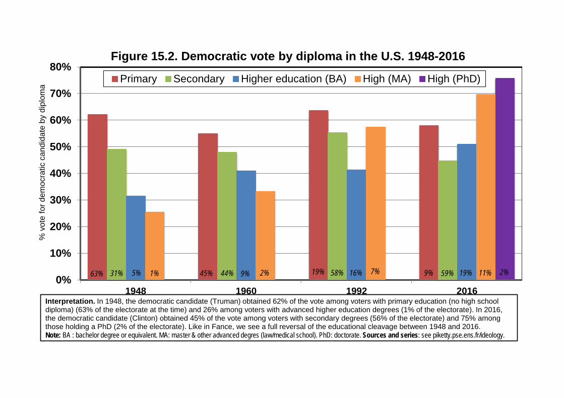
0%
10%
20%
30%
40%
50%
60%
70%
80%
1948 1960 1992 2016
% v
ote
for d
emoc
ratic
can
dida
te b
y di
plom
a
Figure 15.2. Democratic vote by diploma in the U.S. 1948-2016
Primary Secondary Higher education (BA) High (MA) High (PhD)
63% 2%9%44%45%1%31% 5% 7%16%58%19% 2%11%19%59%9%
Interpretation. In 1948, the democratic candidate (Truman) obtained 62% of the vote among voters with primary education (no high school diploma) (63% of the electorate at the time) and 26% among voters with advanced higher education degrees (1% of the electorate). In 2016, the democratic candidate (Clinton) obtained 45% of the vote among voters with secondary degrees (56% of the electorate) and 75% among those holding a PhD (2% of the electorate). Like in Fance, we see a full reversal of the educational cleavage between 1948 and 2016.Note: BA : bachelor degree or equivalent. MA: master & other advanced degres (law/medical school). PhD: doctorate. Sources and series: see piketty.pse.ens.fr/ideology.de l'auteur à partir des enquêtes post électorales 1956 2017 (élections présidentielles et législatives) 1956 les partis de gauche (SFIO PS PCF

-24%-20%-16%-12%
-8%-4%0%4%8%
12%16%20%24%
1945 1950 1955 1960 1965 1970 1975 1980 1985 1990 1995 2000 2005 2010 2015 2020
Figure 15.3. The Democratic vote and education: U.S. 1948-2016
Difference between % Democratic vote among college graduatesand non-college graduatesAfter controls for age, sex, family situation
After controls for age, sex, family situation, income, wealth, race
Interpretation. In 1948, the democratic candidate obtained a score that was 20 points smaller among college graduates than among college graduates; in 2016, this score is 14 points higher among college graduates. Controlling for other variables ("other things equal") does not affect the trend (only the levels). Sources and series: see piketty.pse.ens.fr/ideology.de l'auteur à partir des enquêtes post-électorales 1956-2017 (élections présidentielles et législatives). 1956, les partis de gauche (SFIO-PS, PCF, MRG, divers gauche et écologistes, extrême-gauche) obtiennent un score 12 point

-24%-20%-16%-12%
-8%-4%0%4%8%
12%16%20%24%28%
1945 1950 1955 1960 1965 1970 1975 1980 1985 1990 1995 2000 2005 2010 2015 2020
Figure 15.4. Democratic vote in the U.S. 1948-2016:from the workers' party to the party of the highly educated
Difference between % vote democrat among top 10% highesteducation voters and remaining 90%After controls for age, sexe, family situation
After controls for age, sex, family situation, income, wealth, race
Interpretation. In 1948, the democratic candidate obtained a score that was 21 points smaller among the top 10% highest-education voters than among the remaining 90%; in 2016, this score is 23 points higher among the top 10% highest-education voters. Controlling for other variables ("other things equal") does not affect the trend (only the levels). Sources and series: see piketty.pse.ens.fr/ideology.de l'auteur à partir des enquêtes post-électorales 1956-2017 (élections présidentielles et législatives) 1956 les partis de gauche (SFIO-PS PCF

10%
20%
30%
40%
50%
60%
70%
80%
90%
D1 D2 D3 D4 D5 D6 D7 D8 D9 D10 Top5% Top1%
% v
ote
dem
ocra
t as
a fu
nctio
n of
inco
me
deci
le
Figure 15.5. Political conflict and income: U.S. 1948-2016
1948 1964 1976
1980 2000 2004
2012 2016
Interpretation. In 1964, the democratic candidate obtained 69% of the votes among the voters with the 10% lowest incomes, 37% of the vote among those with the top 10% highest incomes and 22% among top 1% income holders. Generally speaking, the profile of democratic vote is declining with respect to income, especially at the beginning of the period. In 2016, for the first time, the profile is reversed: 59% of the top income decile voters support the democratic candidate. Sources and series: see piketty.pse.ens.fr/ideology.de l'auteur à partir des enquêtes post-électorales 1956-2017 (élections présidentielles et législatives). 1956, les partis de gauche (SFIO-PS, PCF, MRG,

-28%-24%-20%-16%-12%
-8%-4%0%4%8%
12%16%20%24%28%32%
1945 1950 1955 1960 1965 1970 1975 1980 1985 1990 1995 2000 2005 2010 2015 2020
Figure 15.6. Social cleavages and political conflict: U.S. 1948-2016 Difference between % vote democrat among top 10% educationvoters and bottom 90% education voters (after controls)Difference between % vote democrat among top 10% income votersand bottom 90% education voters (after controls)Difference between % vote democrat among top wealth voters andbottom wealth voters (after controls)
Interpretation. During the 1950-1970 period, the democratic vote was associated to voters with the lowest levels of educational degrees and the lowest levels of income and wealth. In the 1980-2010 period it became associated to the voters with the highest degrees. In the 2010-2020 period, it is maybe close to become associated with the highest income and wealth voters. Sources and series: see piketty.pse.ens.fr/ideology.alculs de l'auteur à partir des enquêtes post-électorales 1956-2017 (élections présidentielles et législatives). L t 1956 l i d h (SFIO PS PCF MRG di h é l i ê h ) b i 12 i

0%
10%
20%
30%
40%
50%
60%
70%
80%
90%
100%
1948 1952 1956 1960 1964 1968 1972 1976 1980 1984 1988 1992 1996 2000 2004 2008 2012 2016
% v
ote
dem
ocra
t as
a fu
nctio
n of
eth
nic
cate
gory
Figure 15.7. Political conflict and ethnic identity: U.S. 1948-2016Whites Blacks Latinos/others
Interpretation. In 2016, the democratic candidate obtained 37% of the vote among white voters (70% of the electorate), 89% of the vote among black voters (11% of the electorate) and 64% of the vote among Latinos and other non-whites (19% of the electorate, including 16% for Latinos). In 1972, the democratic candidate obtained 32% of the vote among whites (89% of the electorate), 82% among blacks (10% of the electorate) and 64% among Latinos and other categories (1% of the electorate). Sources and series: see piketty.pse.ens.fr/ideology.alculs de l' t à ti d êt t él t l 1956 2017 (él ti é id ti ll t lé i l ti )

-4%0%4%8%
12%16%20%24%28%32%36%40%44%48%52%
1945 1950 1955 1960 1965 1970 1975 1980 1985 1990 1995 2000 2005 2010 2015 2020
Figure 15.8. Political conflict and racial cleavage: U.S. 1948-2016
Difference between % vote democrat among black/latinos/other votersand among white votersAfter controls for age, sex, familiy situation
After controls for age, sex, family situation, degree, income, wealth
Interpretation. In 1948, the democratic vote was 11 points higher among black and other minority voters (9% of the electorate) than among white voters (91% of the electorate). In 2016, the democratic vote was 39 points higher among black and other minority voters (30%) of the electorate than among wite voters (70% of the electorate). Taking into account control variables has a limited impact on this gap. Sources and series: see piketty.pse.ens.fr/ideology.alculs de l'auteur à partir des enquêtes post-électorales 1956-2017 (élections présidentielles et législatives).

10%
20%
30%
40%
50%
60%
70%
80%
90%
100%
France 2012 Etats-Unis 2016
% v
ote
dem
ocra
t (U
S) o
r soc
ialis
t (Fr
ance
)
Figure 15.9. Political conflict and origins: France & the US
No foreign origin (France); Whites (U.S.)European foreign origins (France); Latinos (U.S.)Extra-European foreign origins (France); Blacks (U.S.)
72%
49%
19% 9% 11%19%70%
49%
77%
37%
64%
89%
Interpretation. In 2012, the socialist candidate in the second round of the French presidential election obtained 49% of the vote among voters with no foreign origin (no reported foreign grand-parent) and among voters with European foreign origins (in practice mostly Spain, Italy, Portugal) and 77% of the vote among voters with extra-European foreign origins (in practice mostly North Africa and Subsaharan Africa). In 2016, the democratic candidate at the U.S. presidential election obtained 37% of the vote among white voters, 64% among latinos and other minority voters and 89% among black voters. Sources and series: see piketty.pse.ens.fr/ideology.alculs de l'auteur à partir des enquêtes post-électorales 1956-2017 (élections présidentielles et législatives).

0%4%8%
12%16%20%24%28%32%36%40%44%48%52%56%
1945 1950 1955 1960 1965 1970 1975 1980 1985 1990 1995 2000 2005 2010 2015 2020
Per
cent
age
of v
otes
obt
aine
d by
the
vario
us p
artie
sFigure 15.10. Legislative elections in Britain 1945-2017
LabourConservatives (Tories)Liberals/Lib-DemSNPUKIPOther parties
Interpretation. In the 1945 legislative elections, the Labour party obtained 48% of the vote and the Conservatives 36% of the vote (hence a total of 84% of the vote for the two main parties). In the 2017 legislative elections, the Conservatives obtained 42% of the vote, and the Labour party 40% of the vote (hence a total of 82%). Note. Liberals/Lib-Dem: Liberals, Liberals-democrats, SDP Alliance. SNP: Scottish National Party. UKIP: UK Independance Party. Other parties include green and regionalist parties. Sources and séries: see piketty.pse.ens.fr/ideology.de l'auteur à partir des enquêtes post électorales 1956 2017 (élections présidentielles et législatives) 1956 les partis de gauche (SFIO PS PCF MRG divers
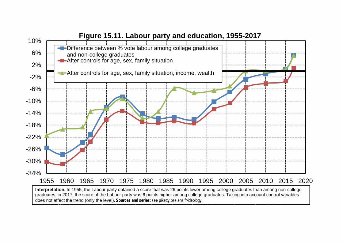
-34%
-30%
-26%
-22%
-18%
-14%
-10%
-6%
-2%
2%
6%
10%
1955 1960 1965 1970 1975 1980 1985 1990 1995 2000 2005 2010 2015 2020
Figure 15.11. Labour party and education, 1955-2017 Difference between % vote labour among college graduatesand non-college graduatesAfter controls for age, sex, family situation
After controls for age, sex, family situation, income, wealth
Interpretation. In 1955, the Labour party obtained a score that was 26 points lower among college graduates than among non-college graduates; in 2017, the score of the Labour party was 6 points higher among college graduates. Taking into account control variables does not affect the trend (only the level). Sources and series: see piketty.pse.ens.fr/ideology.de l'auteur à partir des enquêtes post-électorales 1956-2017 (élections présidentielles et législatives). 1956, les partis de gauche (SFIO-PS, PCF, MRG, divers gauche et écologistes,
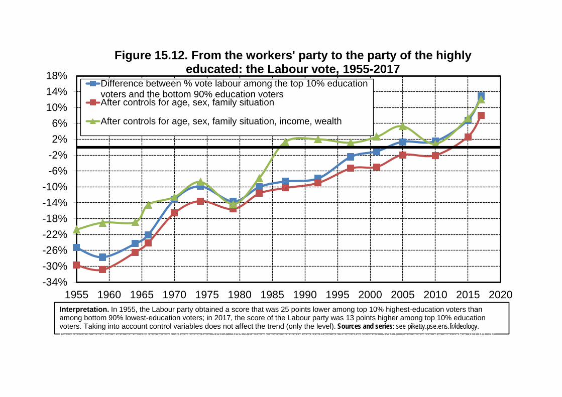
-34%-30%-26%-22%-18%-14%-10%
-6%-2%2%6%
10%14%18%
1955 1960 1965 1970 1975 1980 1985 1990 1995 2000 2005 2010 2015 2020
Figure 15.12. From the workers' party to the party of the highly educated: the Labour vote, 1955-2017
Difference between % vote labour among the top 10% educationvoters and the bottom 90% education votersAfter controls for age, sex, family situation
After controls for age, sex, family situation, income, wealth
Interpretation. In 1955, the Labour party obtained a score that was 25 points lower among top 10% highest-education voters than among bottom 90% lowest-education voters; in 2017, the score of the Labour party was 13 points higher among top 10% education voters. Taking into account control variables does not affect the trend (only the level). Sources and series: see piketty.pse.ens.fr/ideology.de l'auteur à partir des enquêtes post-électorales 1956-2017 (élections présidentielles et législatives). 1956, les partis de gauche (SFIO-PS, PCF MRG di h t é l i t t ê h ) bti t 12 i t

-28%-24%-20%-16%-12%
-8%-4%0%4%8%
12%16%20%24%
1945 1950 1955 1960 1965 1970 1975 1980 1985 1990 1995 2000 2005 2010 2015 2020
Figure 15.13. The electoral left in Europe & the US, 1945-2020: from the workers' party to the party of the highly educated
U.S.: difference among % Democratic vote among top 10% highest-education voters and bottom 90% lowest-education votersFrance: same difference with % vote for left-wing parties
Britain: same difference with % vote for labour party
Interpration. During the 1950-1970 period, the vote for the democratic party in the U.S., left-wing parties in France (socialists-communists-radicals-greens) in France and the labour party in Britain was associated with the voters with the lowest educational diplomas; in the 1990-2010 period is became associated with the voters with the highest education diplomas. The British evolution is slightly lagging behind the French and U.S. evolutions but goes in the same direction. Sources and series: see piketty.pse.ens.fr/ideology.

0%
10%
20%
30%
40%
50%
60%
70%
80%
90%
D1 D2 D3 D4 D5 D6 D7 D8 D9 D10 Top5% Top1%
% v
ote
labo
ur a
s a
func
tion
of in
com
e de
cile
Figure 15.14. Political conflict and income: Britain 1955-2017
1955 1964
1970 1979
1983 1997
2005 2017
Interpretation. The profile of the vote for the labour party as a function of income decile has generally been strongly decreasing, particularly at the level of the 10% highest incomes, and especially from the 1950s to the 1980s. Sources and series: see piketty.pse.ens.fr/ideology.de l'auteur à partir des enquêtes post-électorales 1956-2017 (élections présidentielles et législatives). 1956, les partis de gauche (SFIO-PS, PCF, MRG, d h é l ê h ) b

-32%-28%-24%-20%-16%-12%
-8%-4%0%4%8%
12%16%20%24%
1955 1960 1965 1970 1975 1980 1985 1990 1995 2000 2005 2010 2015 2020
Figure 15.15. Social cleavages & political conflict: Britain 1955-2017Difference between % vote labour among the top 10% education votersand the bottom 90% education voters (after controls)Difference between % vote labour among the top 10% income voters andthe bottom 90% income voters (after controls)Difference between % vote labour among the op wealth voters and thebottom wealth voters (after controls)
Interpretation. The labour vote was associated during the 1950-1980 period to the voters with the highest diplomas and levels of income and wealth; since the 1990s, it became associated to the highest education degrees. Sources and series: see piketty.pse.ens.fr/ideology.

0%
10%
20%
30%
40%
50%
60%
70%
80%
90%
100%
1964 1979 1997 2010 2017
% v
ote
labo
ur a
s a
func
tion
of re
porte
d re
ligio
n
Figure 15.16. Political conflict & religious diversity: Britain 1964-2017
Christians Other religions No religion Muslims
96% 1% 3% 1%67% 31% 5%48%4%43%47%47%4%57%1% 37% 3%3%2%
Interpretation. In 2017, the labour party obtained 39% of the vote among self-reported christian voters (anglicans, other protestants, catholics), 56% among voters reporting other religions (judaism, hinduism, etc., except islam), 54% among voters with no religion and 96% among self-reported muslim voters. Sources and series: see piketty.pse.ens.fr/ideology.

0%
10%
20%
30%
40%
50%
60%
70%
80%
90%
100%
1979 1987 1997 2010 2017
Figure 15.17. Political conflict & ethnic categories, Britain 1979-2017
Whites Africans-Caribbeans Indians-Pakistanis Others
98% 1% 1% 2% 2% 1%94% 3% 2%6%3%89%2%5%3%90%2%96%
Interpretation. In 2017, the labour party obtained 44% of the vote among voters describing themselves as "Whites", 81% among "Africans-Caribbeans", 82% among "Indians-Pakistanis-Bengladeshis" and 69% among "others" (incluidng "Chinese", "Arabs", etc.). In 2017, 5% of the electorate refused to answer to the ethnic question, and 77% among them voted labour . Sources and series: see piketty.pse.ens.fr/ideology.

30%
35%
40%
45%
50%
55%
60%
65%
70%
75%
D1 D2 D3 D4 D5 D6 D7 D8 D9 D10
% v
ote
for R
EM
AIn
in th
e B
rexi
t 201
6 re
fere
ndum
as
a fu
nctio
n of
inco
me,
edu
catio
n de
gree
and
wea
lth d
ecile
Figure 15.18. The European cleavage in Britain: the Brexit referendum in 2016
Remain (income)Remain (education)Remain (wealth)
Interpretation. In the 2016 referendum over Brexit (victory of Leave with 52%), one observes a very strong social cleavage of the vote: the top decoles of income, education and wealth vote strongly for Remain, while bottom deciles vote for Leave. Note: D1 refers to the bottom 10% (either for income, education or wealth), D2 for the next 10%, etc., and D10 for the top 10%. Sources and series: see piketty.pse.ens.fr/ideology.de l'auteur à partir des enquêtes post-électorales 1956-2017 (élections présidentielles et
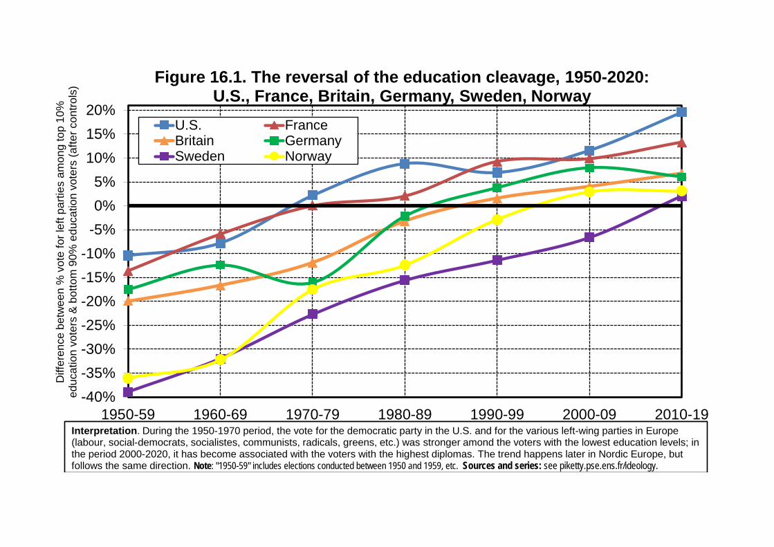
-40%-35%-30%-25%-20%-15%-10%
-5%0%5%
10%15%20%
1950-59 1960-69 1970-79 1980-89 1990-99 2000-09 2010-19
Diff
eren
ce b
etw
een
% v
ote
for l
eft p
artie
s am
ong
top
10%
ed
ucat
ion
vote
rs &
bot
tom
90%
edu
catio
n vo
ters
(afte
r con
trols
) Figure 16.1. The reversal of the education cleavage, 1950-2020: U.S., France, Britain, Germany, Sweden, Norway
U.S. FranceBritain GermanySweden Norway
Interpretation. During the 1950-1970 period, the vote for the democratic party in the U.S. and for the various left-wing parties in Europe (labour, social-democrats, socialistes, communists, radicals, greens, etc.) was stronger amond the voters with the lowest education levels; in the period 2000-2020, it has become associated with the voters with the highest diplomas. The trend happens later in Nordic Europe, but follows the same direction. Note: "1950-59" includes elections conducted between 1950 and 1959, etc. Sources and series: see piketty.pse.ens.fr/ideology.

-25%
-20%
-15%
-10%
-5%
0%
5%
10%
15%
1960-69 1970-79 1980-89 1990-99 2000-09 2010-19
Diff
eren
ce b
etw
een
% v
ote
for l
eft-w
ing
parti
es a
mon
g to
p 10
%
educ
atio
n vo
ters
& b
otto
m 9
0% e
duca
tion
vote
rs (a
fter c
ontro
ls)
Figure 16.2. Political cleavage and education, 1960-2020: Italy, Holland, Switzerland, Canada, Australia, New-Zealand
Italy HollandSwitzerland AustraliaCanada New Zealand
Interpretation. During the 1960-1980 period, the vote for left-wing parties (labour, social-democrats, socialists, communists, radicals, greens, etc.) was associated to the voters with the lowest education levels; in the period 2000-2020, it has become associated to those with the highest diplomas. This general evolution happenned in the U.S. and in Europe, as well as in Canada, Australia and New Zealand. Note: "1960-69" includes elections conducted between 1960 and 1969, "1970-79" those conducted from 1970 to 1979, etc. Sources and series: see piketty.pse.ens.fr/ideology.
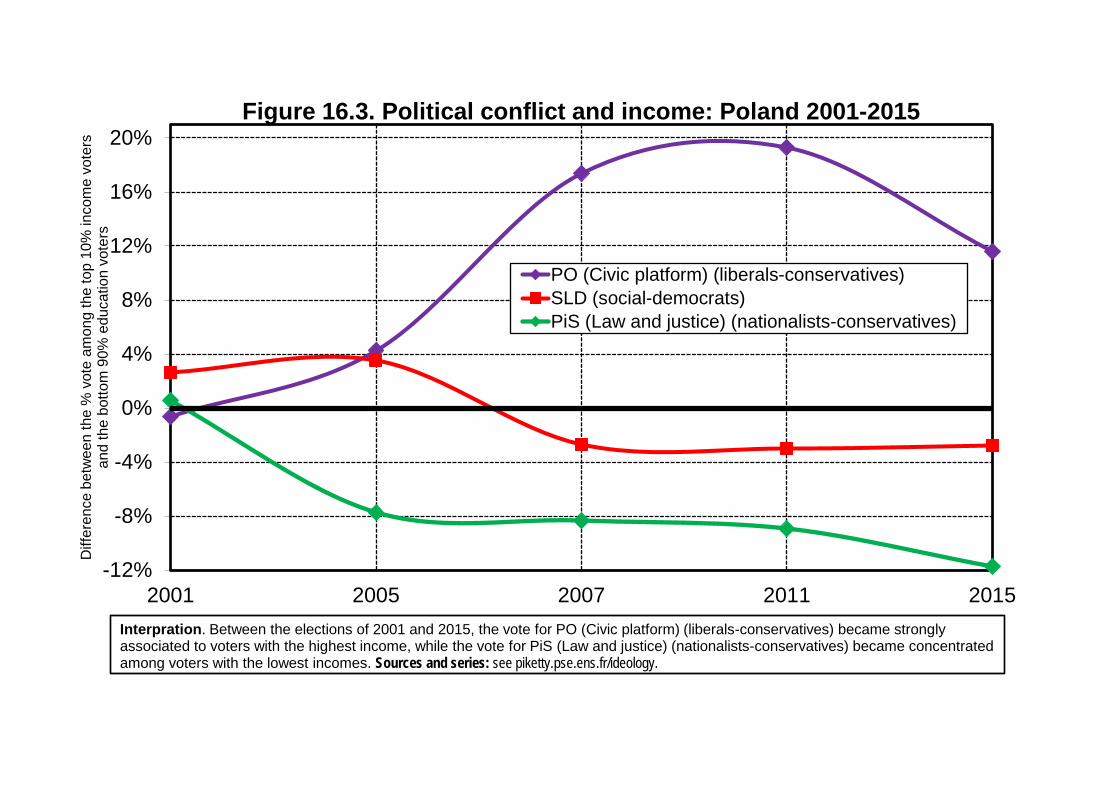
-12%
-8%
-4%
0%
4%
8%
12%
16%
20%
2001 2005 2007 2011 2015
Diff
eren
ce b
etw
een
the
% v
ote
amon
g th
e to
p 10
% in
com
e vo
ters
an
d th
e bo
ttom
90%
edu
catio
n vo
ters
Figure 16.3. Political conflict and income: Poland 2001-2015
PO (Civic platform) (liberals-conservatives)SLD (social-democrats)PiS (Law and justice) (nationalists-conservatives)
Interpration. Between the elections of 2001 and 2015, the vote for PO (Civic platform) (liberals-conservatives) became strongly associated to voters with the highest income, while the vote for PiS (Law and justice) (nationalists-conservatives) became concentrated among voters with the lowest incomes. Sources and series: see piketty.pse.ens.fr/ideology.

-12%
-8%
-4%
0%
4%
8%
12%
16%
2001 2005 2007 2011 2015
Diff
eren
ce b
etw
een
% v
ote
amon
g th
e to
p 10
% e
duca
tion
vote
rs
and
the
botto
m 9
0% e
duca
tion
vote
rs
Figure 16.4. Political conflict and education: Poland 2001-2015PO (Civic platform) (liberals-conservatives)SLD (social-democrats)PiS (Law and justice) (nationalists-conservatives)
Interpretation. Between the elections of 2001 and 2015, the vote for PO (Civic platform) (liberals-conservatives) became associated to voters with the highest education levels, while the vote for PiS (Law and justice) (nationalists-conservatives) became concentrated among voters with the lowest diplomas. Sources and series: see piketty.pse.ens.fr/ideology.

0%
10%
20%
30%
40%
50%
60%
70%
80%
90%
2008 2011 2016
% s
uppo
rt to
gre
ater
regi
onal
aut
onom
y an
d/or
sel
f-det
erm
inat
ion
refe
rend
um (b
oth
resp
onse
s co
mbi
ned)
Figure 16.5. Catalan regionalism and income, 2008-2016
Bottom 50% Nest 40% Top 10%
Interpretation. In 2008, 47% of Catalan voters belonging to the bottom 50% incomes supported greater regional autonomy or a self-determination referendum (both answers were added), vs 64% among the voters with the next 40% incomes and 74% among the top 10% income voters. Sources and series: see piketty.pse.ens.fr/ideology.

0%
10%
20%
30%
40%
50%
60%
70%
80%
90%
2008 2011 2016
% s
uppo
rt to
gre
ater
regi
onal
aut
onom
y an
d/or
sel
f-det
erm
inat
ion
refe
rend
um (b
oth
resp
onse
s co
mbi
ned)
Figure 16.6. Catalan regionalism and education, 2008-2016
Primary Secondary Higher education
Interpretation. In 2008, 44% of Catalan voters with no diploma (except primary education level) supported greater regional autonomy or a self-determination referendum (both answers were added), vs 60% among the voters with secondary degrees and 74% among those withhigher education diplomas. Sources and series: see piketty.pse.ens.fr/ideology.

0%
10%
20%
30%
40%
50%
60%
70%
1960 1965 1970 1975 1980 1985 1990 1995 2000 2005 2010 2015
Per
cent
age
of v
otes
obt
aine
d by
the
vario
us p
artie
sFigure 16.7. Legislative elections in India (Lok Sabha), 1962-2014
Congress (INC) and allied (center) Congress (INC)BJP and allied (right) Left/Center-left partiesOther parties
Interpretation. In the 2014 legislative elections, the Congress party (INC, Indian National Congress) and its allied parties (center) obtained34% of the vote (including 19% for INC alone), the BJP (hindus nationalists) and its allied parties (right) 37% of the vote, the left and center-left parties (SP, BSP, CPUI, etc.) 16% of the vote and other parties 13% of the vote. Note: in the 1977 elections (post-emergency), the Janata Dal included all opponents to INC (from left and right), and it classified here with "other parties". Sources and series: see piketty.pse.ens.fr/ideology.

0%
10%
20%
30%
40%
50%
60%
70%
1962 1967 1971 1996 1998 1999 2004 2009 2014
Vote
BJP
(and
alli
es) a
s a
func
tion
of c
aste
and
relig
ion
Figure 16.8. BJP vote by caste and religion: India 1962-2014
Muslims SC/ST (lower castes) OBC Other FC (upper castes) Brahmins
Interpretation. In 2014, 10% of muslim voters voted for the BJP (hindus nationalists) and allied parties, vs 31% among SC/ST (scheduled castes/ scheduled tribes, lower castes), 42% among OBC (other backward classes, intermediate castes), 49% among other FC (forward castes, upper castes except brahmins) and 61% among brahmins. Sources and series: see piketty.pse.ens.fr/ideology.

0%
10%
20%
30%
40%
50%
60%
70%
1962 1967 1971 1996 1998 1999 2004 2009 2014
Vote
INC
(and
alli
es) a
s a
func
tion
of c
aste
and
relig
ion
Figure 16.9. Congress vote by caste and religion: India 1962-2014
Muslims SC/ST (lower castes) OBC Other FC (upper castes) Brahmins
Interpretation. In 2014, 45% of muslim voters voted for the Congress (Indian National Congress) and allied parties, vs 38% among SC/ST (scheduled castes/ scheduled tribes, lower castes), 34% among OBC (other backward classes, intermediate castes), 27% among other FC (forward castes, upper castes except brahmins) and 18% among brahmins. Sources and series: see piketty.pse.ens.fr/ideology.

0%
5%
10%
15%
20%
25%
30%
35%
40%
1962 1967 1971 1996 1998 1999 2004 2009 2014
Left
vote
as
a fu
nctio
n of
cas
te a
nd re
ligio
nFigure 16.10. Left vote by caste and religion: India 1962-2014
Muslims SC/ST (lower castes) OBC Other FC (upper castes) Brahmins
Interpretation. In 2014, 23% of muslim voters voted for the left and center-left parties (SP, BSP, CPI, etc.), vs 17% among SC/ST (scheduled castes/ scheduled tribes, lower castes), 15% among OBC (other backward classes, intermediate castes), 11% among other FC (forward castes, upper castes except brahmins) and 12% among brahmins. Sources and series: see piketty.pse.ens.fr/ideology.

-4%
0%
4%
8%
12%
16%
20%
24%
28%
32%
1962 1967 1971 1996 1998 1999 2004 2009 2014
Figure 16.11. BJP vote among upper castes, 1962-2014Difference between % vote BJP (and allies) among upper castes (FC) and other votersAfter controls for StateAfter controls for State, age, sex, degree, rural/urban/city size
Interpretation. During the 1962-2014 period, upper caste voters (FC, forward castes) have always voted more than others for the BJP (and allies), before and after taking into account control variables. The impact of caste (after taking into account other variables) appears to have become more important over time. Sources and series: see piketty.pse.ens.fr/ideology.

-20%
-16%
-12%
-8%
-4%
0%
4%
8%
1962 1967 1971 1996 1998 1999 2004 2009 2014
Figure 16.12. BJP vote among lower castes, 1962-2014
Difference between % vote BJP (and allies) among lower castes (SC/ST) and other votersAfter controls for StateAfter controls for State, age, sex, degree, urban/rural/city size
Interpretation. During the 1962-2014 period, lower caste voters (SC/ST, scheduled castes/scheduled tribes) have always voted less than others for the BJP (and allies), before and after taking into account control variables. Sources and series: see piketty.pse.ens.fr/ideology.

-4%
0%
4%
8%
12%
16%
20%
24%
28%
32%
36%
1962 1967 1971 1996 1998 1999 2004 2009 2014
Figure 16.13. The BJP & the religious clevage: India 1962-2014Difference between % vote BJP among hindus (all castes combined) and among muslimsAfter controls for StateAfter controls for State, age, sex, degree, urban/rural/city size
Interpretation. During the 1962-2014 period, hindus voters (all castes combined: SC/ST, OBC and FC) have always voted more than muslim voters for the BJP (and allies), before and after taking into account control variables. The magnitude of the religious clevage has strongly increased over time. Sources and series: see piketty.pse.ens.fr/ideology.

0%
10%
20%
30%
40%
50%
60%
Bihar Gujarat Jharkhand Maharashtra Rajasthan Uttar Pradesh Uttarakhand
Vote
for B
JP (a
nd a
llies
) as
a fu
nctio
n of
cas
te a
nd re
ligio
nFigure 16.14. BJP vote by caste, religion and State: India 1996-2016
Muslims SC/ST (lower castes) OBC FC (upper castes)
Interpretation. In all Indian States, the BJP (and allies) always obtains a higher score among upper castes (FC, forward castes) than amongOBC (other backward classes, intermediate castes), SC/ST (scheduled castes/schedules tribes, lower castes) and muslim voters. Note: the results reported here refer to the average regional elections conducted over the 1996-2016 period. Sources and series: see piketty.pse.ens.fr/ideology.

-12%
-8%
-4%
0%
4%
8%
1989 1994 1998 2002 2006 2010 2014 2018
Figure 16.15. The politisation of inequality in Brasil, 1989-2018Difference between % vote PT among the top 10% highest educationvoters and bottom 90% lowest education voters (after controls)Difference between % vote PT among the top 10% income voters andthe bottom 90% income voters (after controls)
Intepretation. During the 1989-2018 period, the vote in favour of PT (Workers Party) in Brasil has become more and more associated with voters with the lowest levels of income and degrees, which was not the case in the first elections conducted after the end of the military dictatorship. Sources and series: see piketty.pse.ens.fr/ideology.
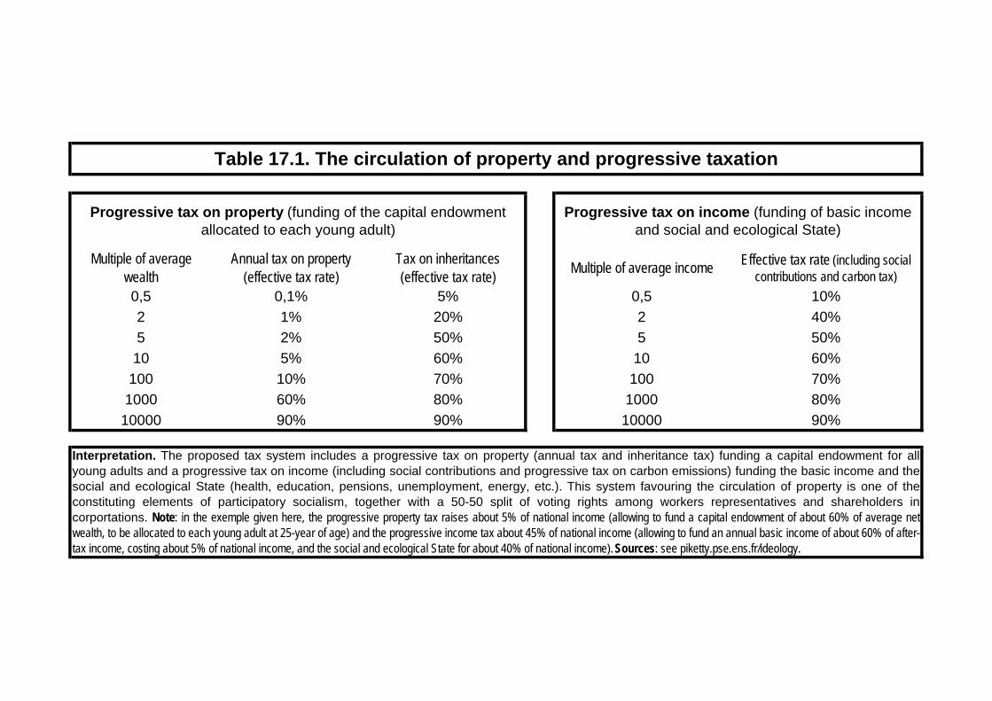
Multiple of average wealth
Annual tax on property (effective tax rate)
Tax on inheritances (effective tax rate) Multiple of average income Effective tax rate (including social
contributions and carbon tax)0,5 0,1% 5% 0,5 10%2 1% 20% 2 40%5 2% 50% 5 50%10 5% 60% 10 60%
100 10% 70% 100 70%1000 60% 80% 1000 80%
10000 90% 90% 10000 90%
Table 17.1. The circulation of property and progressive taxation
Progressive tax on property (funding of the capital endowment allocated to each young adult)
Progressive tax on income (funding of basic income and social and ecological State)
Interpretation. The proposed tax system includes a progressive tax on property (annual tax and inheritance tax) funding a capital endowment for allyoung adults and a progressive tax on income (including social contributions and progressive tax on carbon emissions) funding the basic income and thesocial and ecological State (health, education, pensions, unemployment, energy, etc.). This system favouring the circulation of property is one of theconstituting elements of participatory socialism, together with a 50-50 split of voting rights among workers representatives and shareholders incorportations. Note: in the exemple given here, the progressive property tax raises about 5% of national income (allowing to fund a capital endowment of about 60% of average netwealth, to be allocated to each young adult at 25-year of age) and the progressive income tax about 45% of national income (allowing to fund an annual basic income of about 60% of after-tax income, costing about 5% of national income, and the social and ecological State for about 40% of national income). Sources: see piketty.pse.ens.fr/ideology.

0
50
100
150
200
250
300
0 5 10 15 20 25 30 35 40 45 50 55 60 65 70 75 80 85 90 95Tota
l pub
lic e
duca
tiona
l inv
estm
ent r
ecei
ved
by s
tude
nts
(from
kin
derg
arte
n to
uni
vers
ity) (
thou
sand
s eu
ros
2018
)
Percentile of the distribution of total educational investment received (within a cohort)
Figure 17.1. The inequality of educational investment: France 2018
Interpretation.Total public educational investment received during their studies (from kindergarten to university) by the students of the cohort reaching 18-year-old in 2018 will be about 120 k€ (i.e. approximately 15 years of studies for an average cost of 8000€ per year). Within this generation, the 10% of students receiving the smallest educational investment receive about 65-70 k€, while the 10% receiving the most receive between 200 k€ and 300 k€. Note: average costs per year of study in the French educational system in 2015-2018 rank from 5-6 k€ in kindergarten-primary to 8-10 k€ in secondary, 9-10 k€ in universities and 15-16 k€ in preparatory classes to grandes ecoles (etlite tracks).Sources and series: see piketty.pse.ens.fr/ideology.et

Table 17.2. A novel organisation of globalisation: transnational democracy
Interpretation. According to the proposed organisation, the treaties regulating globalisation (flows of goods, capital and individuals) will henceforth include the creation between the signatories States and Regional Unions of a Transnational Assembly in charge of global public goods (climate, research, etc.) and global fiscal justice (common taxes on high wealth and income holders and large corporations, carbon taxes). Note. Countries A, B, C, D can be States like France, Germany, Italy, Spain, etc., in which case the Transational Assembly will be the European Assembly; or countries A, B, etc. could be Regional Unions like the European Union, the African Union, etc., in which case the Transnational Assembly would be that of the Euro-African Union. The Transnational Assembly could be formed of deputies from the National Assemblies and/or of transnational deputies especially elected for this purpose, depending on the situation. Sources: see piketty.pse.ens.fr/ideology.
National Assembly Country D
National Assembly Country A
National Assembly Country B
National Assembly Country C …
Transnational Assembly In charge of global public goods (climate, research, etc.) and of global fiscal justice (common taxes on high
wealth and income holders and large corporations, carbon taxes)