Teaching a Machine to Read Maps with Deep Reinforcement Learning

Gino Brunner and Oliver Richter and Yuyi Wang and Roger Wattenhofer∗ETH Zurich

{brunnegi, richtero, yuwang, wattenhofer}@ethz.ch

Abstract

The ability to use a 2D map to navigate a complex 3D envi-ronment is quite remarkable, and even difficult for many hu-mans. Localization and navigation is also an important prob-lem in domains such as robotics, and has recently become afocus of the deep reinforcement learning community. In thispaper we teach a reinforcement learning agent to read a mapin order to find the shortest way out of a random maze it hasnever seen before. Our system combines several state-of-the-art methods such as A3C and incorporates novel elementssuch as a recurrent localization cell. Our agent learns to lo-calize itself based on 3D first person images and an approx-imate orientation angle. The agent generalizes well to biggermazes, showing that it learned useful localization and naviga-tion capabilities.

1 IntroductionOne of the main success factors of human evolution is ourability to craft and use complex tools. Not only did thisability give us a motivation for social interaction by teach-ing others how to use different tools, it also enhanced ourthinking capabilities, since we had to understand ever morecomplex tools. Take a map as an example; a map helps usnavigate places we have never seen before. However, wefirst need to learn how to read it, i.e., we need to asso-ciate the content of a two-dimensional map with our three-dimensional surroundings. With algorithms becoming in-creasingly capable of learning complex relations, a way tomake machines intelligent is to teach them how to use al-ready existing tools. In this paper, we teach a machine howto read a map with deep reinforcement learning.

The agent wakes up in a maze. The agent’s view is an im-age: the maze rendered from the agent’s perspective, like adungeon in a first person video game. This rendered imageis provided by the DeepMind Lab environment (Beattie etal. 2016). The agent can be controlled by a human, or asin our case, by a complex deep reinforcement learning ar-chitecture.1 The agent can move (forward, backward, left,right) and rotate (left, right), and its view image will change

∗Names in alphabetic orderCopyright c© 2018, Association for the Advancement of ArtificialIntelligence (www.aaai.org). All rights reserved.

1Our code can be found here: https://github.com/OliverRichter/map-reader.git

accordingly. In addition, the agent gets to see a map of themaze, also an image, as can be seen in Figure 1. One loca-tion on the map is marked with an “X” - the agent’s target.The crux is that the agent does not know where on the map itcurrently is. Several locations on the map might correspondwell with the current view. Thus the agent needs to movearound to learn its position and then move to the target, asillustrated in Figures 6 and 8. We do equip the agent with anapproximate orientation angle, i.e., the agent roughly knowsthe direction it is moving or looking. In the map, up is alwaysnorth. During training the agent learns which approximateorientation corresponds to north.

A complex multi-stage task, such as navigating a mazewith the help of a map, can be naturally decomposed intoseveral subtasks: (i) The agent needs to observe its 3D en-vironment and compare it to the map to determine its mostlikely position. (ii) The agent needs to understand the map,or in our case associate symbols on the map with rewardsand thereby gain an understanding of what a wall is, whatnavigable space is, and what the target is. (iii) Finally theagents needs to learn how to follow a plan in order to reachthe target.

Our contribution is as follows: We present a novel modu-lar reinforcement learning architecture that consists of a re-active agent and several intermediate subtask modules. Eachof these modules is designed to solve a specific subtask. Themodules themselves can contain neural networks or alter-natively implement exact algorithms or heuristics. Our pre-sented agent is capable of finding the target in random mazesroughly three times the size of the largest mazes it has seenduring training.

Further contributions include:

• The Recurrent Localization Cell that outputs a locationprobability distribution based on an estimated stream ofvisible local maps.

• A simple mapping module that creates a visible local 2Dmap from 3D RGB input. The mapping module is robust,even if the agent’s compass is inaccurate.

2 Related WorkReinforcement learning in relation to AI has been stud-ied since the 1950’s (Minsky 1954). Important early workon reinforcement learning includes the temporal difference

learning method by Sutton (1984; 1988), which is the ba-sis for actor-critic algorithms (Barto, Sutton, and Anderson1983) and Q-learning techniques (Watkins 1989; Watkinsand Dayan 1992). First works using artificial neural net-works for reinforcement learning include (Williams 1992)and (Gullapalli 1990). For an in-depth overview of rein-forcement learning we refer the interested readers to (Kael-bling, Littman, and Moore 1996), (Sutton and Barto 1998)and (Szepesvari 2010).

The current deep learning boom was started by, amongother contributions, the backpropagation algorithm (Rumel-hart et al. 1988) and advances in computing power and GPUframeworks. However, deep learning could not be appliedeffectively to reinforcement learning until recently. Mnih etal. (2015) introduced the Deep-Q-Network (DQN) that usesexperience replay and target networks to stabilize the learn-ing process. Since then, several extensions to the DQN ar-chitecture have been proposed, such as the Double Deep-Q-Network (DDQN) (van Hasselt, Guez, and Silver 2016)and the dueling network architecture (Wang et al. 2016).These networks are based on using replay buffers to stabilizelearning, such as prioritized experience replay (Schaul et al.2015). The state-of-the-art A3C (Mnih et al. 2016) relies onasynchronous actor-learners to stabilize learning. In our sys-tem, we use A3C learning on a modified network architec-ture to train our reactive agent and the localization modulein an on-policy manner. We also make use of (prioritized)replay buffers to train our agent off policy.

A major challenge in reinforcement learning are environ-ments with delayed or sparse rewards. An agent that nevergets a reward can never learn good behavior. Thus Jaderberget al. (2016) and Mirowski et al. (2016) introduced auxiliarytasks that let the agent learn based on intermediate intrin-sic pseudo-rewards, such as predicting the depth from a 3DRGB image, while simultaneously trying to solve the maintask, e.g., finding the exit in a 3D maze. The policies learnedby the auxiliary tasks are not directly used by the agent, butsolely serve the purpose of helping the agent learn betterrepresentations which improves its performance on the maintask. The idea of auxiliary tasks is inspired by prior workon temporal abstractions, such as options (Sutton, Precup,and Singh 1999), whose focus was on learning temporal ab-stractions to improve high-level learning and planning. Inour work we introduce a modularized architecture that in-corporates intermediate subtasks, such as localization, localmap estimation and global map interpretation. In contrastto (Jaderberg et al. 2016), our reactive agent directly usesthe outputs of these modules to solve the main task. Notethat we use an auxiliary task inside our localization moduleto improve the local map estimation. Kulkarni et al. (2016)introduced a hierarchical version of the DQN to tackle thechallenge of delayed and sparse rewards. Their system oper-ates at different temporal scales and allows the definition ofgoals using entity relations. The policy is learned in such away to reach these goals. We use a similar approach to makeour agent follow a plan, such as, “go north”.

Mapping and localization has been extensively studied inthe domain of robotics (Thrun, Burgard, and Fox 2005).A robot creates a map of the environment from sensory

input (e.g., sonar or LIDAR) and then uses this map toplan a path through the environment. Subsequent workshave combined these approaches with computer vision tech-niques (Fuentes-Pacheco, Ascencio, and Rendon-Mancha2015) that use RGB(-D) images as input. Machine learningtechniques have been used to solve mapping and planningseparately, and later also tackled the joint mapping and plan-ning problem (Elfes 1989). Instead of separating mappingand planning phases, reinforcement learning methods aimedat directly learning good policies for robotic tasks, e.g., forlearning human-like motor skills (Peters and Schaal 2008).

Recent advances in deep reinforcement learning havespawned impressive work in the area of mapping and lo-calization. The UNREAL agent (Jaderberg et al. 2016) usesauxiliary tasks and a replay buffer to learn how to navi-gate a 3D maze. Mirowski et al. (2016) came up with anagent that uses different auxiliary tasks in an online man-ner to understand if navigation capabilities manifest as a bi-product of solving a reinforcement learning problem. Zhuet al. (2017) tackled the problems of generalization acrosstasks and data inefficiency. They use a realistic 3D environ-ment with physics engine to gather training data efficiently.Their model is capable of navigating to a visually specifiedtarget. In contrast to other approaches, they use a memory-less feed-forward model instead of recurrent models. Guptaet al. (2017) simulated a robot that navigates through a real3D environment. They focus on the architectural problem oflearning mapping and planning in a joint manner, such thatthe two phases can profit from knowing each other’s needs.Their agent is capable of creating an internal 2D represen-tation of the local 3D environment, similar to our local vis-ible map. In our work a global map is given, and the agentlearns to interpret and read that map to reach a certain tar-get location. Thus, our agent is capable of following com-plicated long range trajectories in an approximately shortestpath manner. Furthermore, their system is trained in a fullysupervised manner, whereas our agent is trained with rein-forcement learning. Bhatti et al. (2016) augment the stan-dard DQN with semantic maps in the VizDoom (Kempka etal. 2016) environment. These semantic maps are constructedfrom 3D RGB-D input, and they employ techniques suchas standard computer vision based object recognition andSLAM. They showed that this results in better learned poli-cies. The task of their agent is to eliminate as many oppo-nents as possible before dying. In contrast, our agent needsto escape from a complex maze. Furthermore, our environ-ments are designed to provide as little semantic informationas possible to make the task more difficult for the agent; ouragent needs to construct its local visible map based purelyon the shape of its surroundings.

3 ArchitectureMany complex tasks can be divided into easier intermediatetasks which when all solved individually solve the complextask. We use this principle and apply it to neural network ar-chitecture design. In this section we first introduce our con-cept of modular intermediate tasks, and then discuss howwe implement the modular tasks in our map reading archi-tecture.

Visible Local Map Network

Recurrent Localization Cell

at-1 rt-1

Map Interpretation Network

Reactive Agent

V

{piloc}N

i=1

{piloc}N

i=1rt-1

STTD

? Hloc

Figure 1: Architecture overview and interplay between thefour modules. α is the discretized angle, at−1 is the last ac-tion taken, rt−1 is the last reward received, {ploci }Ni=1 is theestimated location probability distribution over the N pos-sible discrete locations, H loc is the entropy of the estimatedlocation probability distribution, STTD is the short term tar-get direction suggested by the map interpretation network, Vis the estimated state value and π is the policy output fromwhich the next action at is sampled.

3.1 Modular Intermediate TasksAn intermediate task module can be any information pro-cessing unit that takes as input either sensory input and/orthe output of other modules. A module is defined and de-signed after the intermediate task it solves and can consistof trainable and hard coded parts. Since we are dealing withneural networks, the output and therefore the input of a mod-ule can be erroneous. Each module adjusts its trainable pa-rameters to reduce its error independent of other modules.We achieve this by stopping error back-propagation on mod-ule boundaries. Note that this separation has some advan-tages and drawbacks:

• Each module performance can be evaluated and debuggedindividually.

• Small intermediate subtask modules have short credit as-signment paths, which reduces the problem of explodingand vanishing gradients during back-propagation.

• Modules cannot adjust their output to fit the input needs ofthe next module. This has to be achieved through interfacedesign, i.e., intermediate task specification.

Our neural network architecture consists of four mod-ules, each dedicated to a specific subtask. We first give anoverview of the interplay between the modules before de-scribing them in detail in the following sections. The archi-tecture overview is sketched in Figure 1.

The first module is the visible local map network; it takesthe raw visual input from the 3D environment and creates foreach frame a two dimensional map excerpt of the currentlyvisible surroundings. The second module, the recurrent lo-calization cell, takes the stream of visible local map excerpts

CNN CNN

Visible LocalMap

FC

FC

FC

FC

Visual Input

Visible Field

MapExcerpt

Figure 2: The visible local map network: The RGB pixelinput is passed through two convolutional neural network(CNN) layers and a fully connected (FC) layer before be-ing concatenated to the discretized angle α and further pro-cessed by fully connected layers and a gating operation.

and integrates it into a local map estimation. This local mapestimation is compared to the global map to get a probabil-ity distribution over the discretized possible locations. Thethird module is called map interpretation network; it learnsto interpret the global map and outputs a short term targetdirection for the estimated position. The last module is a re-active agent that learns to follow the estimated short termtarget direction to ultimately find the exit of the maze.

We allow our agent to have access to a discretized angleα describing the direction it is facing, comparable to a robothaving access to a compass. Furthermore, we do not limitourself to completely unsupervised learning and allow theagent to use a discretized version of its actual position duringtraining. This could be implemented as a robot training onthe network with the help of a GPS signal. The robot couldtrain as long as the accuracy of the GPS signal is below acertain threshold and act on the trained network as soon asthe GPS signal gets inaccurate or totally lost. We leave sucha practical implementation of our algorithm to future workand focus here on the algorithmic structure itself.

We now describe each module architecture individuallybefore we discuss their joint training in Section 3.6. If notspecified otherwise, we use rectified linear unit activationsafter each layer.

3.2 Visible Local Map NetworkThe visible local map network preprocesses the raw visualRGB input from the environment through two convolutionalneural network layers followed by a fully connected layer.We adapted this preprocessing architecture from (Jaderberget al. 2016). The thereby generated features are concate-nated to a 3-hot discretized encoding α of the orientationangle α, i.e., we input the angle as n-dimensional vectorwhere each dimension represents a discrete state of the an-gle, with n = 30. We set the three vector components thatrepresent the discrete angle values closest to the actual angleto one while the remaining components are set to zero, e.g.α = [0 . . . 01110 . . . 0]. We used a 3-hot instead of a 1-hotencoding to smooth the input. Note that this encoding has anaverage quantization error of 6 degrees.

The discretized angle and preprocessed visual features arepassed through a fully connected layer to get an intermediaterepresentation from which two things are estimated:

at-1

rt-1

{piloc}Ni=1

V

st-1

FC

FC

softmax

st

M

softmax

∑

.

LMest

LMmfb

LMest+mfb

~

Figure 3: Sketch of the information flow in the recurrent lo-calization cell. The last egomotion estimation st−1, the dis-cretized angle α, the last action at−1 and reward rt−1 arepassed through two fully connected (FC) layers and com-bined with a two dimensional convolution between the for-mer local map estimation LMest

t−1 and the current visible lo-cal map input to get the new egomotion estimation st. Thisegomotion estimation is used to shift the previously esti-mated local map LMest

t−1 and the previous map feedback lo-cal map LMmfb

t−1 . A weighted and clipped combination ofthese local map estimations, LMest+mfb

t−1 , is convolved withthe full map to get the estimated location probability dis-tribution {ploci }Ni=1. Recurrent connections are marked byempty arrows.

1. A reconstruction of the map excerpt that corresponds tothe current visual input

2. The current field of view, which is used to gate the esti-mated map excerpt such that only estimates which lie inthe line of sight make it into the visible local map. Thisgating is crucial to reduce noise in the visible local mapoutput.

See Figure 2 for a sketch of the visible local map networkarchitecture.

3.3 Recurrent Localization CellMoving around in the environment, the agent generates astream of visible local map excerpts like the output in Fig-ure 2 or the visible local map input V in Figure 3. The recur-rent localization cell then builds an egocentric local map outof this stream and compares it to the actual map to estimate

the current position. The agent has to predict its egomotionto shift the egocentric estimated local map accordingly. Werefer to Figure 3 for a sketch of the architecture describedhereafter.

Let M be the current map, V the output of the visible lo-cal map network, α the discretized 3-hot encoded orientationangle, at−1 the 1-hot encoded last action taken, rt−1 the ex-trinsic reward received by taking action at−1, LMest

t the es-timated local map at time step t, LMmfb

t the map feedbacklocal map at time step t, LMest+mfb

t the estimated localmap with map feedback at time step t, st the estimated nec-essary shifting (or estimated egomotion) at time step t and{ploci }Ni=1 the discrete estimated location probability distri-bution. Then we can describe the functionality of the recur-rent localization cell by the following equations:

st = softmax(f(st−1, α, at−1, rt−1) + LMestt−1 ∗ V )

LMestt =

[LMest

t−1 ∗ st + V]+0.5

−0.5

LMest+mfbt =

[LMest

t + λ · LMmfbt−1 ∗ st

]+0.5

−0.5

{ploci }Ni=1 = softmax(m ∗ LMest+mfb

t

)LMmfb

t =

N∑i=1

pi · g(m, i)

Here, f(·) is a two layer feed forward neural network,∗ denotes a two dimensional discrete convolution withstride one in both dimensions, [·]+0.5

−0.5 denotes a clipping to[−0.5,+0.5], λ is a trainable map feedback parameter andg(m, i) extracts from the map m the local map around loca-tion i.

3.4 Map Interpretation NetworkThe goal of the map interpretation network is to find reward-ing locations on the map and construct a plan to get to theselocations. We achieve this in three stages: First, the networkpasses the map through two convolutional layers followedby a rectified linear unit activation to create a 3-channel re-ward map. The channels are trained (as discussed in Sec-tion 3.6) to represent wall locations, navigable locations andtarget locations respectively. This reward map is then areaaveraged, rectified and passed to a parameter free 2D short-est path planning module which outputs for each of the dis-crete locations on the map a distribution over {North, East,South, West}, i.e., a short term target direction (STTD),as well as a measure of distance to the nearest target loca-tion. This plan is then multiplied with the estimated locationprobability distribution to get the smooth STTD and targetdistance of the currently estimated location. Note that plan-ning for each possible location and querying the plan withthe full location probability distribution helps to resolve theexploitation-exploration dilemma of the reactive agent:• An uncertain location probability distribution close to the

uniform distribution will result in an uncertain STTD dis-tribution over {North, East, South, West}, thereby encour-aging exploration.

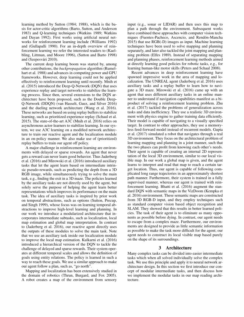
• A location probability distribution over locations withsimilar STTD will accumulate these similarities and re-sult in a clear STTD for the agent, even though the loca-tion might still be unclear (exploitation).

3.5 Reactive Agent and Intrinsic RewardAs mentioned, the reactive agent faces two partially con-tradicting goals: following the STTD (exploitation) and im-proving the localization by generating information rich vi-sual input (exploration), e.g., no excessive staring at walls.The agent learns this trade off through reinforcement learn-ing, i.e., by maximizing the expected sum of rewards. Therewards we provide here are extrinsic rewards from the en-vironment (negative reward for running into walls, positivereward for finding the target) as well as intrinsic rewardslinked to the short term goal inputs of the reactive agent.These short term goal inputs are the STTD distribution over{North, East, South, West} and the measure of distance tothe nearest target location from the map interpretation net-work as well as the normalized entropy H loc of the discretelocation probability distribution {ploci }Ni=1. H loc representsa measure of location uncertainty which is linked to the needfor exploration.

The intrinsic reward consists of two parts to encourageboth exploration and exploitation. The exploration intrinsicreward Iexplort in each timestep t is the difference in locationprobability distribution entropy to the previous timestep:

Iexplort = H loct−1 −H loc

t

Note that this reward is positive if and only if the loca-tion probability distribution entropy decreases, i.e., when theagent gets more certain about its position.

The exploitation intrinsic reward should be a measureof how well the egomotion of the agent aligns with theSTTD. For this we calculate an approximate two dimen-sional egomotion vector ~et from the egomotion proba-bility distribution estimation st. Similarly we calculatea STTD vector ~dt−1 from the STTD distribution over{North,East, South,West} of the previous timestep. Wecalculate the exploitation intrinsic reward Iexploitt as dotproduct between the two vectors:

Iexploitt = ~etT · ~dt−1

Note that this reward is positive if and only if the angledifference between the two vectors is no bigger than 90 de-grees, i.e., if the estimated egomotion was in the same direc-tion as suggested by the STTD in the timestep before.

As input to the reactive agent we concatenate the dis-cretized 3-hot angle α, the last extrinsic reward and the loca-tion probability distribution entropy H loc to the STTD dis-tribution and the estimated target distance. The agent itself isa simple feed-forward network consisting of two fully con-nected layers with rectified linear unit activation followed bya fully connected layer for the policy and a fully connectedlayer for the estimated state value respectively. The agentsnext action is sampled from the softmax-distribution overthe policy outputs.

3.6 Training LossesTo train our agent, we use a combination of on-policy losses,where the data is generated from rollouts in the environment,and off-policy losses, where we sample the data from a re-play memory. More specifically, the total loss is the sum ofthe four module specific losses:

1. Lvlm, the off-policy visible local map loss2. Lloc, the on-policy localization loss3. Lrm, the off-policy reward map loss and4. La, the on-policy reactive agents acting lossWe train our agent as asynchronous advantage actor critic,or A3C, with additional losses; similar to DeepMind’s UN-REAL agent (Jaderberg et al. 2016):

In each training iteration, every thread rolls out up to 20steps in the environment and accumulates the localizationloss Lloc and acting loss La. For each step, an experienceframe is pushed to an experience history buffer of fixedlength. Each experience frame contains all inputs the net-work requires as well as the current discretized true posi-tion. From this experience history, frames are sampled andinputs replayed through the network to calculate the visiblelocal map loss Lvlm and the reward map loss Lrm. We nowdescribe each loss in more detail.

The output V of the visible local map network is trainedto match the visible excerpt of the map V , constructed fromthe discretized location and angle. In each training iteration20 experience frames are uniformly sampled from the expe-rience history and the visible local map loss is calculated asthe sum of L2 distances between visible local map outputsVk and targets Vk:

Lvlm =∑k∈S

||Vk − Vk||2

Here, S denotes the set of sampled frame indices.Our localization loss Lloc is trained on the policy roll-

outs in the environment. For each step, we compare the es-timated position to the actual position in two ways, whichresults in a cross entropy location loss Lloc,xent and a dis-tance location loss Lloc,d. The cross entropy location loss isthe cross entropy between the location probability distribu-tion {ploci }Ni=1 and a 1-hot encoding of the actual position.The distance loss Lloc,d is calculated at each step as the L2distance between the actual two dimensional cell positioncoordinates ~cpos and the estimated centroid of all possiblecells i weighted by their corresponding probability ploci :

Lloc,d =

∣∣∣∣∣∣∣∣∣∣~cpos −

N∑i=1

ploci · ~ci

∣∣∣∣∣∣∣∣∣∣2

In addition to training the location estimation directly wealso assign an auxiliary local map loss Lloc,lm to help withthe local map construction. We calculate the local map lossonly once per training iteration as L2 distance between thelast estimated local map LMest and the actual local map atthat point in time.

The goal of the reward map loss Lrm is to have the threechannels of the reward map represent wall locations, free

0 1 2 3 4 5 6

·106

0

1,000

2,000

3,000

Total Training Steps

Step

sM

ovin

gA

vera

ge

Figure 4: Training performance of 8 actor threads that starttraining on 5x5 mazes. The vertical black lines mark jumpsto larger mazes of the thread in blue.

space locations and target locations respectively. To do this,we leverage the setting that running into a wall gives a nega-tive extrinsic reward, moving in open space gives no extrin-sic reward and finding the target gives a positive extrinsicreward. Therefore the problem can be transformed into esti-mating an extrinsic reward. Each training iteration we sam-ple 20 frames from the experience history. This sampling isindependent from the visible local map loss sampling andskewed to have in expectation equally many frames withpositive, negative and zero extrinsic reward. For each frame,the frames map is passed through the convolution layersof the map interpretation network to create the correspond-ing reward map while the visual input and localization statesaved in the frame are fed through the network to get theestimated location probability distribution. The reward maploss is the cross entropy prediction error of the reward at theestimated position.

Our reactive agent’s acting loss is equivalent to the A3Clearning described by Mnih et al. (2016). We also adaptedan action repeat of 4 and a frame rate of 15 fps. The wholenetwork is trained by RMSprop gradient descent with gra-dient back propagation stopped at module boundaries, i.e.,each module is only trained on its module specific loss.

4 Environment and ResultsTo evaluate our architecture we created a training and testset of mazes with the corresponding black and white mapsin the DeepMind Lab environment. The mazes are quadraticgrid mazes with each maze cell being either a wall, an openspace, the target or the spawn position. The training set con-sists of 100 mazes of different sizes; 20 mazes each in thesizes 5x5, 7x7, 9x9, 11x11 and 13x13 maze cells. The testset consists of 900 mazes; 100 in each of the sizes 5x5, 7x7,9x9, 11x11, 13x13, 15x15, 17x17, 19x19 and 21x21. Notethat the outermost cells in the mazes are always walls, there-fore the maximal navigable space of a 5x5 maze is 3x3 mazecells. Thus the navigable space for the biggest test mazes isroughly 3 times larger than for the biggest training mazes.

For the localization, we used a location cell granularity3 times finer than the maze cells, which results in a totalof N=63x63=3969 discrete location states on the biggest

5 7 9 11 13 15 17 19 21

0

2,000

4,000

Maze width

Step

sne

eded

Figure 5: All the results of the (at most 100) successful testsfor each maze size. Every single test is represented by an“x”. The line connects the arithmetic averages of each mazesize. The distance between origin and target grows linearlywith maze size, as does the number of steps.

21x21 mazes. We train our agent starting on small mazesand increase the maze sizes as the agent gets better. Morespecifically we use 16 asynchronous agent training threadsfrom which we start 8 on the smallest (5x5) training mazeswhile the other training threads are started 2 each on theother sizes (7x7, 9x9, 11x11 and 13x13). This prevents thevisible local map network from overfitting on the small 5x5mazes. The thread agents are placed into a randomly sam-pled maze of their currently associated maze size and try tofind the exit, while counting their steps. A step is one inter-action with the environment, i.e., sampling an action fromthe agents policy π and receiving the corresponding next vi-sual input, discretized angle and extrinsic reward from theenvironment. A step is not the same as a location or mazegrid cell; as agents accelerate, there is no direct correlationbetween steps and actual walked distance. We consider eachsampled maze an episode start. The episode ends success-fully if the agent manages to find the target and the stepsneeded are stored. If the agent does not find the exit in 4500steps, the episode ends as not successful. After an episodeends, a new episode is started, i.e., a new maze is sampled.Note that in this setting the agent is always placed in a newlysampled maze and not in the same maze as in (Jaderberg etal. 2016) and (Mirowski et al. 2016).

For each thread we calculate a moving average of stepsneeded to end the episodes. Once this moving average fallsbelow a maze size specific threshold, the thread is trans-ferred to train on mazes of the next bigger size. Once athread’s moving average of steps needed in the biggest train-ing mazes (13x13) falls below the threshold, the thread isstopped and its training is considered successful. Once allthreads reach this stage, the overall training is consideredsuccessful and the agent is fully trained. We calculate themoving average over the last 50 episodes and use 60, 100,140, 180 and 220 steps as threshold for the maze sizes 5x5,7x7, 9x9, 11x11 and 13x13, respectively. Figure 4 shows thetraining performance of 8 actor threads. One can see that theagents sometimes overfit their policies which results in tem-porarily decreased performance even though the maze sizedid not increase. In the end however, all threads reach goodperformance.

The trained agent is tested on the 900 test set mazes, the

Maze size 5x5 7x7 9x9 11x11 13x13 15x15 17x17 19x19 21x21Targets found 100% 100% 100% 99% 99% 98% 93% 93% 91%

Table 1: Percentage of targets found in the test mazes. Up to size 9x9 the agent always finds the target. More interestingly, theagent is able to find more than 90% of the targets in mazes that are bigger than any maze it has seen during training.

1 2

3 4

Figure 6: Example trajectories walked by the agent. Notethat the agent walks close to the shortest path and its contin-uous localization and planning lets the agent find the path tothe target even after it took a wrong turn.

5 7 9 11 13 15 17 19 210

500

Maze width

Step

sne

eded

Figure 7: Comparison of our agent (blue lines) to an agentthat has perfect position information and an optimal shortterm target direction input (red lines). The solid lines countall steps (turns and moves). The solid blue line is the same asthe average line of Figure 5. The dashed lines do not countthe steps in which the agent turns. The figure shows that theoverhead is mostly because of turning, as our agent needs to“look around” to localize itself.

number of required steps per maze size are plotted in Fig-ure 5. We stop a test after 4,500 steps, but even for thebiggest test mazes (21x21) the agent found more than 90%of the targets within these 4,500 steps. See Table 1 for thepercentage of exits found in all maze sizes.

If the agent finds the exit it does so in almost shortestpath manner, as can be seen in Figure 6. However, the agentneeds a considerable number of steps to localize itself. Toevaluate this localization overhead, we trained an agent con-sisting solely of the reactive agent module with access to theperfect location and optimal short term target direction andplotted its average performance on the test set in Figure 7.The figure shows a large gap between the full agent and theagent with access to the perfect position. This is due to turn-ing actions, which the full agent performs to localize itself,

1 2 3 4

Figure 8: Four example frames to illustrate the typical be-havior of the agent: The red line is the trace of its actualposition, while the shades of blue represent its position esti-mate. The darker the blue, the more confident the agent is tobe in this location. Frame 1 shows the agent’s true startingposition as a red dot, frame 2 shows several similar locationsidentified after a bit of turning, in frame 3 the agent starts tounderstand the true location, and in frame 4 it has moved.

i.e., it continuously needs to look around to know where it is.For the localization in the beginning of an episode, the agentalso mainly relies on turning as can be seen in four exampleframes in Figure 8.

5 ConclusionWe have presented a deep reinforcement learning agent thatcan localize itself on a 2D map based on observations ofits 3D surroundings. The agent manages to find the exit inmazes with high success rate, even in mazes substantiallylarger than it has ever seen during training. The agent oftenfinds the shortest path, showing that the agent can continu-ously retain a good localization.

The architecture of our system is built in a modular fash-ion. Each module deals with a subtask of the maze prob-lem and is trained in isolation. This modularity allows fora structured architecture design, where a complex task isbroken down into subtasks, and each subtask is then solvedby a module. Modules consist of general architectures, e.g.,MLPs, or more task-specific networks such as our recurrentlocalization cell. It is also possible to use deterministic algo-rithm modules, such as in our shortest path planning module.Architecture design is aided by the possibility to easily re-place each module by ground truth values, if available, tofind sources of bad performance.

Our agent is designed for a specific task. We plan to makeour modular architecture more general and apply it to othertasks, such as playing 3D games. Since modules can beswapped out and arranged differently, it would be interestingto equip an agent with many modules and let it learn whichmodule to use in which situation.

AcknowledgmentsWe would like to thank the anonymous reviewers for theirhelpful comments.

ReferencesBarto, A. G.; Sutton, R. S.; and Anderson, C. W. 1983. Neu-ronlike adaptive elements that can solve difficult learningcontrol problems. IEEE Trans. Systems, Man, and Cyber-netics 13(5):834–846.Beattie, C.; Leibo, J. Z.; Teplyashin, D.; Ward, T.; Wain-wright, M.; Kuttler, H.; Lefrancq, A.; Green, S.; Valdes, V.;Sadik, A.; Schrittwieser, J.; Anderson, K.; York, S.; Cant,M.; Cain, A.; Bolton, A.; Gaffney, S.; King, H.; Hassabis,D.; Legg, S.; and Petersen, S. 2016. Deepmind lab. CoRRabs/1612.03801.Bhatti, S.; Desmaison, A.; Miksik, O.; Nardelli, N.; Sid-dharth, N.; and Torr, P. H. S. 2016. Playing doomwith slam-augmented deep reinforcement learning. CoRRabs/1612.00380.Elfes, A. 1989. Using occupancy grids for mobile robotperception and navigation. IEEE Computer 22(6):46–57.Fuentes-Pacheco, J.; Ascencio, J. R.; and Rendon-Mancha,J. M. 2015. Visual simultaneous localization and mapping:a survey. Artif. Intell. Rev. 43(1):55–81.Gullapalli, V. 1990. A stochastic reinforcement learning al-gorithm for learning real-valued functions. Neural Networks3(6):671–692.Gupta, S.; Davidson, J.; Levine, S.; Sukthankar, R.; and Ma-lik, J. 2017. Cognitive mapping and planning for visualnavigation. CoRR abs/1702.03920.Jaderberg, M.; Mnih, V.; Czarnecki, W. M.; Schaul, T.;Leibo, J. Z.; Silver, D.; and Kavukcuoglu, K. 2016. Rein-forcement learning with unsupervised auxiliary tasks. CoRRabs/1611.05397.Kaelbling, L. P.; Littman, M. L.; and Moore, A. W. 1996.Reinforcement learning: A survey. J. Artif. Intell. Res.4:237–285.Kempka, M.; Wydmuch, M.; Runc, G.; Toczek, J.; andJaskowski, W. 2016. Vizdoom: A doom-based AI researchplatform for visual reinforcement learning. In IEEE Confer-ence on Computational Intelligence and Games, CIG 2016,Santorini, Greece, September 20-23, 2016, 1–8.Kulkarni, T. D.; Narasimhan, K.; Saeedi, A.; and Tenen-baum, J. 2016. Hierarchical deep reinforcement learning:Integrating temporal abstraction and intrinsic motivation. InAdvances in Neural Information Processing Systems 29: An-nual Conference on Neural Information Processing Systems2016, December 5-10, 2016, Barcelona, Spain, 3675–3683.Minsky, M. L. 1954. Theory of neural-analog reinforce-ment systems and its application to the brain model problem.Princeton University.Mirowski, P.; Pascanu, R.; Viola, F.; Soyer, H.; Ballard,A. J.; Banino, A.; Denil, M.; Goroshin, R.; Sifre, L.;Kavukcuoglu, K.; Kumaran, D.; and Hadsell, R. 2016.Learning to navigate in complex environments. CoRRabs/1611.03673.Mnih, V.; Kavukcuoglu, K.; Silver, D.; Rusu, A. A.; Veness,J.; Bellemare, M. G.; Graves, A.; Riedmiller, M. A.; Fidje-land, A.; Ostrovski, G.; Petersen, S.; Beattie, C.; Sadik, A.;Antonoglou, I.; King, H.; Kumaran, D.; Wierstra, D.; Legg,

S.; and Hassabis, D. 2015. Human-level control throughdeep reinforcement learning. Nature 518(7540):529–533.Mnih, V.; Badia, A. P.; Mirza, M.; Graves, A.; Lillicrap,T. P.; Harley, T.; Silver, D.; and Kavukcuoglu, K. 2016.Asynchronous methods for deep reinforcement learning.CoRR abs/1602.01783.Peters, J., and Schaal, S. 2008. Reinforcement learningof motor skills with policy gradients. Neural Networks21(4):682–697.Rumelhart, D. E.; Hinton, G. E.; Williams, R. J.; et al. 1988.Learning representations by back-propagating errors. Cog-nitive modeling 5(3):1.Schaul, T.; Quan, J.; Antonoglou, I.; and Silver, D. 2015.Prioritized experience replay. CoRR abs/1511.05952.Sutton, R. S., and Barto, A. G. 1998. Reinforcement learn-ing - an introduction. Adaptive computation and machinelearning. MIT Press.Sutton, R. S.; Precup, D.; and Singh, S. P. 1999. Betweenmdps and semi-mdps: A framework for temporal abstractionin reinforcement learning. Artif. Intell. 112(1-2):181–211.Sutton, R. S. 1984. Temporal credit assignment in reinforce-ment learning.Sutton, R. S. 1988. Learning to predict by the methods oftemporal differences. Machine Learning 3:9–44.Szepesvari, C. 2010. Algorithms for Reinforcement Learn-ing. Synthesis Lectures on Artificial Intelligence and Ma-chine Learning. Morgan & Claypool Publishers.Thrun, S.; Burgard, W.; and Fox, D. 2005. Probabilisticrobotics. MIT press.van Hasselt, H.; Guez, A.; and Silver, D. 2016. Deep rein-forcement learning with double q-learning. In Proceedingsof the Thirtieth AAAI Conference on Artificial Intelligence,February 12-17, 2016, Phoenix, Arizona, USA., 2094–2100.Wang, Z.; Schaul, T.; Hessel, M.; van Hasselt, H.; Lanctot,M.; and de Freitas, N. 2016. Dueling network architec-tures for deep reinforcement learning. In Proceedings of the33nd International Conference on Machine Learning, ICML2016, New York City, NY, USA, June 19-24, 2016, 1995–2003.Watkins, C. J., and Dayan, P. 1992. Q-learning. Machinelearning 8(3-4):279–292.Watkins, C. J. C. H. 1989. Learning from delayed rewards.Ph.D. Dissertation, King’s College, Cambridge.Williams, R. J. 1992. Simple statistical gradient-followingalgorithms for connectionist reinforcement learning. Ma-chine Learning 8:229–256.Zhu, Y.; Mottaghi, R.; Kolve, E.; Lim, J. J.; Gupta, A.; Fei-Fei, L.; and Farhadi, A. 2017. Target-driven visual naviga-tion in indoor scenes using deep reinforcement learning. In2017 IEEE International Conference on Robotics and Au-tomation, ICRA 2017, Singapore, Singapore, May 29 - June3, 2017, 3357–3364.